Cosmological quantum entanglement : A possible testbed for the existence of Kalb-Ramond field

Abstract

In the present paper, we explore the possible effects of a second rank antisymmetric tensor field, known as Kalb-Ramond (KR) field, on cosmological particle production as well as on quantum entanglement for a massive scalar field propagating in a four dimensional FRW spacetime evolves through a symmetric bounce. For this purpose, the scalar field is considered to be coupled with the KR field and also with the Ricci scalar via the term $\sim\xi R\Phi^{2}$ (with $\xi$ be the coupling). The presence of KR field spoils the conformal symmetry of a massless scalar field even for $\xi=1/6$ in four dimensional context, which has interesting consequences on particle production and consequently on quantum entanglement as we will discuss. In particular, the presence of KR field in a FRW bouncing universe allows a greater particle production and consequently the upper bound of the entanglement entropy becomes larger in comparison to the case when the KR field is absent. This may provide an interesting testbed for the existence of Kalb-Ramond field in our universe.

I Introduction

The inflationary paradigm guth ; starobinsky ; linde1 ; linde2 ; rubakov ; lyth is one of the two most successful scenarios that can consistently describe the primordial era of our Universe, while the second scenario being that of the bounce cosmologybrandenberger . Both scenarios can predict a nearly scale invariant power spectrum and a small amount of gravitational radiation, which are also verified and tightly constrained by the latest Planck planck . Despite the enormous successes, a consistent cosmological model is still riddled with some questions like (1) the late time acceleration of our universe acc1 ; acc2 implying that most of the content of the universe is some form of dark energy whose nature remains unknown to us, (2) the mystery of dark matter remains elusive inspite of the latest progress of the Large Hadron Collider in the context of elementary Particle Physics aad1 ; aad2 ; vk1 ; vk2 .

Another important ingredient for a cosmological model (more generally in the context of gravity) is missing: we do not fully understand the nature of quantum gravity responsible for early universe phenomena like inflation or bouncing. Without a generally accepted quantum theory of gravity where the backreaction of quantum fields on the curvature of spacetime should be taken into account, the quantum field theory in a curved spacetime without the backreaction is normally considered so far davies . In this regard, the dynamics of the background spacetime has non-trivial effects on quantum fields propagating on that spacetime when compared with their flat spacetime counterparts. In particular, the interaction of a quantum scalar field with a time dependent classical FRW spacetime excites a definite number of scalar particles from an infinite-past-vacuum-state and consequently the particles become quantum entangled in the asymptotic future ball ; fuentes ; steeg ; genovese ; martinez1 ; martinez2 ; martinez3 ; pierini1 ; pierini2 ; pierini3 ; nakai . Such entanglement may be quantified by von-Neumann or Renyi entropy nakai , however in the present paper we stick to the von-Neumann entropy. Moreover it is shown that such quantum correlations may be present today as a remnant of the primitive universe and can provide precise information about the nature and history of the underlying spacetime martinez3 ; pierini3 ; pierini4 . Thus their study may prove useful in constructing the early universe models. Motivated by this idea, here we try to explore the possible effects of a string inspired second rank antisymmetric tensor field, known as Kalb-Ramond (KR) field, on cosmological scalar particle production as well as on quantum entanglement between the particles produced with a hope that the entanglement entropy may provide a possible testbed for the existence of the KR field in our universe (see kalb ; callan for some of the seminal works on Kalb-Ramond field).

This string-inspired term is motivated by the fact that during the primordial epoch, quantum gravity or string theory effects may have a significant imprint on the evolution of the Universe, so in our case we quantify the quantum epoch’s imprint on the evolution of the Universe, by using this rank two KR antisymmetric tensor field. In general, antisymmetric tensor fields or equivalently p-forms, constitute the field content of all superstring models, and in effect these can actually have a realistic impact in the low-energy limit of the theory buchbinder . Apart from the string theory view point, the KR field also plays significant role in many other places as well, some of them are given by :

• Modified theories of gravity, formulated using twistors, require the inclusion of this antisymmetric tensor field howe1 ; howe2 .

• Attempts to unify gravity and electromagnetism necessitates the inclusion of Kalb-Ramond field in higher-dimensional theories kubyshin ; german .

• Spacetime endowed with Kalb-Ramond field becomes optically active exhibiting birefringence kar1 ; kar2 .

• In majumdar an antisymmetric tensor field $B_{\mu\nu}$ identified to be the Kalb-Ramond field was shown to act as the source of spacetime torsion.

Most importantly, in the context of cosmology, the KR field energy density is found to decrease as $1/a^{6}$ (with $a$ being the scale factor of our universe) with the expansion of our universe tp1 ; tp2 ; tp3 i.e at a faster rate in comparison to radiation and matter components. Thus as the Universe evolves and cools down, the contribution of the KR field on the evolutionary process reduces significantly, and at present it almost does not affect the evolution. However the KR field has a significant contribution during early universe (when the scale factor is small), in particular, it affects the beginning of inflation as well as increases the amount of primordial gravitational radiation and hence enlarges the value of tensor to scalar ratio in respect to the case when the KR field is absent. The important question that ramains is:

• Sitting in present day universe, how do we confirm the existence of the Kalb-Ramond field which has considerably low energy density (with respect to the other components) in our present universe ?

The answer to this question may be encripted in some late time phenomena which carries the information of early universe. One of such phenomena can be the “Cosmological Quantum Entanglement”. Keeping this in mind, here we try to address the possible effects of KR field on cosmological particle production as well as on quantum entanglement for a massive scalar field propagating in a four dimensional FRW spacetime.
The paper is organized as follows: in section II, we present the model and the evolution of classical fields. Section III is reserved for scalar field quantization, calculation of Bogolyubov coefficients, cosmological scalar particle production and quantum entanglement entropy between the produced particles in presence of Kalb-Ramond field and their possible consequences. We finally end the paper with some concluding remarks.

II The model and the evolution of classical fields

In the present paper, we are interested on quantum evolution of a massive scalar field in the bckground of FRW spacetime along with a second rank antisymmetric tensor field, generally known as Kalb-Ramond (KR) field. In particular, our main goal is to determine how the presence of KR field affects the scalar field particle production and the quantum entanglement entropy between the scalar particles. The scalar field coupled with KR field action is given by,

$$S=\int d^{4}x\sqrt{-g}\bigg{[}\frac{1}{2}g^{\mu\nu}\partial_{\mu}\partial_{\nu}\Phi-\frac{1}{2}m^{2}\Phi^{2}-\frac{1}{2}\xi R\Phi^{2}-\frac{1}{12}H_{\mu\nu\alpha}H^{\mu\nu\alpha}-\frac{\alpha}{2}f(\Phi)H_{\mu\nu\alpha}H^{\mu\nu\alpha}\bigg{]}$$ (1)

where $\Phi$ is the scalar field with $m$ is its mass and $H_{\mu\nu\alpha}(=\partial_{[\mu}B_{\nu\alpha]})$ is the field strength tensor of the KR field $B_{\mu\nu}$. Needless to say, first and fourth terms of the above action represent the kinetic terms of th scalar field and the KR field respectively. Moreover the scalar field is non-minimally coupled with gravity and also coupled to $H_{\mu\nu\alpha}$ via the function $f(\Phi)$. In the absence of KR field, the case, $m=0$ and $\xi=1/6$ yields a conformally invariant theory. However it is clear that the presence of KR field breaks the conformal symmetry even for $m=0$ and $\xi=1/6$ because of the coupling function $f(\Phi)$, which has some interesting consequences on particle production and quantum entanglement entropy of the scalar field, as will be discussed later.
Here the spacetime and the KR field are considered as classical fields while the scalar field ($\Phi(x^{\mu})$) is quantized in this background. In this section, we determine the classical evolution of the KR field while the quantization of $\Phi$ ( coupled with the KR field ) is reserved for the next section.
As mentioned earlier, the background classical spacetime is the spatially flat FRW one i.e the metric is given by,

$$ds^{2}=dt^{2}-a^{2}(t)\big{[}dx^{2}+dy^{2}+dz^{2}\big{]},$$ (2)

with $t$ and $a(t)$ being the cosmic time and the scale factor respectively. Transforming cosmic time to conformal time ($\eta$) by $d\eta=\frac{dt}{a(t)}$, the above spacetime metric can be written as,

$$ds^{2}=a^{2}(\eta)\big{[}d\eta^{2}-dx^{2}-dy^{2}-dz^{2}\big{]}.$$ (3)

It is evident that the FRW spacetime with ($\eta$, x, y, z) coordinate system (known as conformal coordinate ) is conformally connected to Minkowski (or flat) spacetime represented by the same coordinate system.

Before presenting the field equations, we want to note that due to the totally antisymmetric nature, $H_{\mu\nu\alpha}$ has four independent components in a four dimensional spacetime, which can be expressed as follows:

$$H_{012}=h_{1}~{}~{}~{}~{}~{}~{}~{}~{}~{}~{}~{}~{},~{}~{}~{}~{}~{}~{}~{}~{}~{}~{}~{}~{}H^{012}=h^{1}$$

$$H_{013}=h_{2}~{}~{}~{}~{}~{}~{}~{}~{}~{}~{}~{}~{},~{}~{}~{}~{}~{}~{}~{}~{}~{}~{}~{}~{}H^{013}=h^{2}$$

$$H_{023}=h_{3}~{}~{}~{}~{}~{}~{}~{}~{}~{}~{}~{}~{},~{}~{}~{}~{}~{}~{}~{}~{}~{}~{}~{}~{}H^{023}=h^{3}$$

$$H_{123}=h_{4}~{}~{}~{}~{}~{}~{}~{}~{}~{}~{}~{}~{},~{}~{}~{}~{}~{}~{}~{}~{}~{}~{}~{}~{}H^{123}=h^{4}$$ (4)

At this stage, it is worth mentioning that due to the presence of the four independent components, the KR field tensor $H_{\mu\nu\alpha}$ can be equivalently expressed by a vector field (which has also four independent components in four dimensions) as $H_{\mu\nu\alpha}=\varepsilon_{\mu\nu\alpha\beta}f^{-1}(\Phi)\Upsilon^{\beta}$ with $\Upsilon^{\beta}$ being the vector field. By virtue of eqn.(4), the off-diagonal Einstein’s equations become,

$$h_{4}h^{3}=h_{4}h^{2}=h_{4}h^{1}=h_{2}h^{3}=h_{1}h^{3}=h_{1}h^{2}=0,$$

which have the following solution

$$h_{1}=h_{2}=h_{3}=0~{}~{}~{}~{}~{}~{}~{},~{}~{}~{}~{}~{}~{}~{}h_{4}\neq 0$$

Thus out of the four independent components of $H_{\mu\nu\alpha}$, only one component i.e $H_{123}=h_{4}$ comes with non trivial solution (other three become trivially zero, which is also in agreement with the isotropic condition of the spacetime). This solution along with the equivalence of $H_{\mu\nu\alpha}$ with the vector field $\Upsilon^{\beta}$, one finds that $\Upsilon^{\beta}$ has also only one non zero component. As a consequence, in a spatially flat FRW spacetime (where the off-diagonal components of Einstein tensor vanish ), $\Upsilon^{\beta}$ can be expressed as a derivative of a massless scalar field $Z(x^{\mu})$ (i.e $\Upsilon^{\beta}=\partial^{\beta}Z$ where $Z(x)$ is known as axion field), which further relates the KR field tensor with the axion field in the following way,

$$H^{\mu\nu\lambda}=\epsilon^{\mu\nu\lambda\beta}f^{-1}(\Phi)\partial_{\beta}Z.$$ (5)

With the help of eqn.(5), the equation of motion for KR field can be obtained as,

$$\frac{d}{d\eta}\bigg{[}f^{-1}(\Phi)\frac{dZ}{d\eta}\bigg{]}+2\frac{\dot{a}}{a}\bigg{[}f^{-1}(\Phi)\frac{dZ}{d\eta}\bigg{]}=0.$$ (6)

The above differential equation can be integrated once to yeild,

$$\frac{dZ}{d\eta}\propto f(\Phi)/a^{2}.$$ (7)

Using the above expression, we determine the KR field energy density ($\rho_{KR}$) in terms of the scale factor $a(\eta)$ as follows,

$$\rho_{KR}=\frac{1}{2}h_{4}h^{4}=\frac{1}{2}g^{00}\bigg{[}f^{-1}(\Phi)\frac{dZ}{d\eta}\bigg{]}^{2}=\frac{h_{0}}{a^{6}}$$ (8)

with $h_{0}$ being an integration constant which must take only positive values in order to get a real valued solution for $h_{4}(t)$. In addition, eqn.(8) clearly indicates that the energy density of the KR field ($\rho_{KR}$) is proportional to $1/a^{6}$ and in effect, $\rho_{KR}$ decreases as the Universe expands, in a faster rate in comparison to matter ($\propto 1/a^{3}$) and radiation ($\propto 1/a^{4}$) energy densities respectively.
With the classical evolution of KR field in hand, we now discuss the possible effects of KR field on the scalar field quantization, scalar particle production, entanglement entropy between the scalar particles etc.

III Scalar field quantization, Bogolyubov coefficients, scalar particle production and entanglement entropy in the presence of KR field

The action in eqn.(1) leads to the scalar field ($\Phi$) equation as,

$$\bigg{[}\Box_{g}+m^{2}+\xi R\bigg{]}\Phi+\alpha\rho_{KR}f^{\prime}(\Phi)=0,$$ (9)

where $f^{\prime}(\Phi)=\frac{df}{d\Phi}$ and recall $\rho_{KR}=\frac{1}{2}H_{\mu\nu\lambda}H^{\mu\nu\lambda}=\frac{1}{2}h_{4}h^{4}$. The coupling $f(\Phi)$ is the term that carries the imprint of the KR field on scalar field quantization. Without the coupling term (i.e for $\alpha=0$), the scalar field quantization is unaffected by the KR field evolution, which is also evident from eqn.(9). However the scalar field is propagating in FRW spacetime charted by conformal coordinate system, for which the box operator takes the form

$$\Box_{g} = \frac{1}{\sqrt{-g}}\partial_{\mu}\bigg{[}\sqrt{-g}g^{\mu\nu}\partial_{\nu}\bigg{]}$$ (10)

$$= \frac{1}{a^{4}}\bigg{[}\frac{\partial}{\partial\eta}\bigg{(}a^{4}g^{00}\frac{\partial}{\partial\eta}\bigg{)}+\frac{\partial}{\partial x}\bigg{(}a^{4}g^{11}\frac{\partial}{\partial x}\bigg{)}+\frac{\partial}{\partial y}\bigg{(}a^{4}g^{22}\frac{\partial}{\partial y}\bigg{)}+\frac{\partial}{\partial z}\bigg{(}a^{4}g^{33}\frac{\partial}{\partial z}\bigg{)}\bigg{]}$$

$$= \frac{1}{a^{2}}\bigg{[}\frac{\partial^{2}}{\partial\eta^{2}}-\nabla^{2}+\frac{2\dot{a}}{a}\frac{\partial}{\partial\eta}\bigg{]}.$$

where an overdot represents derivative with respect to the conformal time i.e $\frac{d}{d\eta}$. Expanding the field $\Phi$ in Fourier modes as,

$$\Phi(\vec{x},\eta) = \int d^{3}k\Phi_{\vec{k}}(\vec{x},\eta)$$ (11)

$$= \int d^{3}k\bigg{[}\frac{1}{(2\pi)^{3/2}}e^{i\vec{k}.\vec{x}}\frac{\chi_{k}(\eta)}{a(\eta)}\bigg{]},$$

where we also introduce the auxiliary field $\chi_{k}(\eta)=a(\eta)\Phi(\eta)$. With such auxiliary field, we simplify the term $\Box_{g}\Phi_{\vec{k}}$ to yeild -

$$\Box_{g}\Phi_{\vec{k}}=e^{i\vec{k}.\vec{x}}\bigg{[}\frac{1}{a^{3}}\big{(}\ddot{\chi}_{k}+k^{2}\chi_{k}\big{)}-\frac{1}{6}R(\eta)\chi_{k}\bigg{]},$$ (12)

with $R(\eta)=6\ddot{a}/a^{3}$ being the scalar curvature of the spacetime and $\ddot{\chi}_{k}=\frac{d^{2}\chi_{k}}{d\eta^{2}}$ (recall the overdot stands for $\frac{d}{d\eta}$ as mentioned after Eq.(10)). Now in order to get an explicit form of the scalar field equation, the coupling function $f(\Phi)$ is taken as quadratic one i.e

$$f(\Phi)=\Phi^{2}/2.$$ (13)

Such quadratic form of the coupling function leads to the scalar field equation as similar to harmonic oscillator like equation (with time dependent frequency, as we will see below in eqn.(14)), which in turn makes the scalar field quantization easier. Plugging the expression of $\Box_{g}\Phi_{\vec{k}}$ into eqn.(9) and using the quadratic form of $f(\Phi)$, one obtains the following equations of motion for the modes $\chi_{k}(\eta)$ :

$$\ddot{\chi}_{k}+\bigg{[}k^{2}+\big{(}\xi-\frac{1}{6}\big{)}R(\eta)a^{2}(\eta)+m^{2}a^{2}(\eta)+\frac{\alpha h_{0}}{a^{4}}\bigg{]}\chi_{k}(\eta)=0,$$ (14)

where we use the solution of $\rho_{KR}=h_{0}/a^{6}$ (see eqn.(8)).
It is evident that the mode functions get decoupled in the above equation of motion. Such decoupling of the field modes hinges on the separation of the time coordinate in the Klein-Gordon equation and on the Fourier expansion of the field $\Phi$ through the eigenfunctions of the spatial Laplace operator at a fixed time. It may be mentioned that the field equations in a general spacetime are not separable. In such cases, the mode decoupling cannot be performed explicitly and quantization is difficult. However this is not the subject of our present paper and thus without going into details of the quantization in a general spacetime, we keep our focus on that in the expanding FRW spacetime in presence of KR field.

III.1 Quantization of the scalar field

In order to quantize the scalar field, $\chi_{k}(\eta)$ is replaced by the field operator i.e $\hat{\chi}_{k}(\eta)$ and $\hat{\Psi}_{k}(\vec{x},\eta)=e^{i\vec{k}.\vec{x}}\hat{\chi}_{k}(\eta)$ satisfies the following equal time commutation relation,

$$\bigg{[}\hat{\Psi}_{k}(\vec{x},\eta),\hat{\pi}_{k}(\vec{x},\eta)\bigg{]}=i\delta(\vec{x}-\vec{y}),$$ (15)

with $\hat{\pi}_{k}(\vec{x},\eta)=\frac{d\hat{\Psi}_{k}(\vec{x},\eta)}{d\eta}$ be the canonical momentum conjugate to $\hat{\Psi}_{k}(\vec{x},\eta)$. The quantum Hamiltonian comes with the following expression,

$$\hat{H}_{k}(\eta)=\frac{1}{2}\int d^{3}x\bigg{[}\hat{\pi}_{k}^{2}+(\nabla\hat{\Psi}_{k})^{2}+m_{eff}^{2}(\eta)\hat{\Psi}_{k}^{2}(\vec{x},\eta)\bigg{]}$$ (16)

with $m_{eff}^{2}(\eta)=\big{(}\xi-\frac{1}{6}\big{)}R(\eta)a^{2}(\eta)+m^{2}a^{2}(\eta)+\frac{\alpha h_{0}}{a^{4}}$, known as effective mass of the field mode. The Hamiltonian $\hat{H}_{k}(\eta)$ resembles with a harmonic oscillator Hamiltonian except the fact that the mass term here explicitly depends on time, which in turn makes the Hamiltonian explicit time dependent. This time dependence arises due to the interaction of the scalar field with the background time dependent gravitational field (i.e FRW spacetime). The expression of $\hat{H}$ along with the Fourier decomposition of $\hat{\Psi}_{k}(\vec{x},\eta)$ lead to the Heisenberg equation for $\hat{\chi}_{k}(\eta)$ as follows,

$$\frac{d^{2}\hat{\chi}_{k}}{d\eta^{2}}+\bigg{[}k^{2}+\big{(}\xi-\frac{1}{6}\big{)}R(\eta)a^{2}(\eta)+m^{2}a^{2}(\eta)+\frac{\alpha h_{0}}{a^{4}}\bigg{]}\hat{\chi}_{k}(\eta)=0,$$ (17)

where we use the explicit form of $m_{eff}^{2}(\eta)$. It is evident that the form of eqn.(17) resembles with that of eqn.(14). However this is expected as Heisenberg equation resembles to the corresponding classical field equation with the replacement of the “classical field” by the “field operator”.
Till now, we did not consider any particular form of the scale factor ($a(\eta)$), but in order to proceed further, we do need a certain form of $a(\eta)$ and thus we choose a suitable form of the background FRW spacetime as follows,

$$a(\eta)=1-\frac{\sigma^{2}}{2\big{(}\eta^{2}+\sigma^{2}\big{)}},$$ (18)

with $\sigma$ being the model parameter. The above form of the scale factor corresponds to a non-singular symmetric bounce at $\eta=0$. Such form of the scale factor has also been used earlier in pierini3 to study the possible effects of spacetime anisotropy on cosmological entanglement. At this stage it deserves mention that here, in the present paper, we choose this certain form of the scale factor in order to make the calculations easier. However we will show that our final argument regarding the testbed of KR field through entanglement entropy remains valid for the class of scale factor (irrespective of a particular form) which exhibits a symmetric bounce.
Eqn.(18) leads to $a(\pm\infty)=1$ which in turn admits an asymptotically flat spacetime. In order to reveal the asymptotic nature of spacetime more clearly, we rewrite eqn.(17) in the following form,

$$\frac{d^{2}\hat{\chi}_{k}}{d\eta^{2}}+\bigg{[}\omega_{k}^{2}-V_{k}(\eta)\bigg{]}\hat{\chi}_{k}(\eta)=0,$$ (19)

where $\omega_{k}^{2}=k^{2}+m^{2}+\alpha h_{0}$ and

$$V_{k}(\eta)=m^{2}\big{[}1-a^{2}(\eta)\big{]}-\big{(}\xi-\frac{1}{6}\big{)}R(\eta)a^{2}(\eta)+\alpha h_{0}\bigg{[}1-\frac{1}{a^{4}(\eta)}\bigg{]}.$$ (20)

The above expression clearly demonstrates that for a flat background spacetime (i.e for $a(\eta)=1$), $V_{k}(\eta)$ becomes trivially zero. In the present context, $V_{k}(\eta)$ attains a non-zero value because the FRW spacetime is a “curved” spacetime, and moreover it encodes the information of the interaction of the scalar field with the background time dependent gravitational field. This is the reason that $V_{k}(\eta)$ is generally known as potential term or interaction term. Eqn.(20) further entails that $V_{k}(\eta)$ consists of three parts - the first one is proportional to $m^{2}$, the second one is proportional to $(\xi-1/6)$ while the third part arises due to the presence of KR field and depends on $h_{0}$. The term $R(\eta)a^{2}(\eta)\sim\frac{3\eta^{2}-\sigma^{2}}{(\eta^{2}+\sigma^{2})^{2}(2\eta^{2}+\sigma^{2})}$ goes to zero for $\eta\rightarrow\pm\infty$ and thus the interaction term $V_{k}(\eta)$ also approaches to zero asymptotically. Thereby eqn.(19) clearly demonstrates that the mode operator $\hat{\chi}_{k}(\eta)$ obeys the flat spaceime like equation in the regime $\eta\rightarrow\pm\infty$ with $\omega_{k}^{2}=k^{2}+m^{2}+\alpha h_{0}$. As a consequence - if $\zeta_{k}^{(in)}(\eta)$ and $\zeta_{k}^{(out)}(\eta)$ are the mode solutions of eqn.(19), which are consistent with the correct vacuum of the scalar field at $\eta\rightarrow\mp\infty$ respectively, then such mode solutions come with the following asymptotic behaviour,

$$\zeta_{k}^{(in)}(\eta\rightarrow-\infty)=\frac{1}{\sqrt{2\omega_{k}}}e^{-i\omega_{k}\eta}$$

$$\zeta_{k}^{(out)}(\eta\rightarrow+\infty)=\frac{1}{\sqrt{2\omega_{k}}}e^{-i\omega_{k}\eta}$$ (21)

$\zeta_{k}^{(in)}(\eta)$ and $\zeta_{k}^{(out)}(\eta)$ are known as “in-mode” and “out-mode” solution respectively. Moreover $\hat{\chi}_{k}(\eta)$ can be written as linear combination (as eqn.(19) is linear in $\chi_{k}$) of these mode solutions as follows :

$$\hat{\chi}_{k}(\eta) = \hat{a}_{\vec{k}}\zeta_{k}^{(in)*}(\eta)+\hat{a}_{-\vec{k}}^{+}\zeta_{k}^{(in)}(\eta)$$ (22)

$$= \hat{b}_{\vec{k}}\zeta_{k}^{(out)*}(\eta)+\hat{b}_{-\vec{k}}^{+}\zeta_{k}^{(out)}(\eta),$$

where $\hat{a}_{\vec{k}}$ and $\hat{b}_{\vec{k}}$ are operator coefficients which obey commutation relations like - $[\hat{a}_{\vec{k}},\hat{a}^{+}_{\vec{k^{\prime}}}]=\delta(\vec{k}-\vec{k^{\prime}})$ , $[\hat{b}_{\vec{k}},\hat{b}^{+}_{\vec{k^{\prime}}}]=\delta(\vec{k}-\vec{k^{\prime}})$ and all other commutators are zero. Such operator coefficients actually represent the annihilation operator for in ($\eta\rightarrow-\infty$) and out ($\eta\rightarrow+\infty$) region respectively. Thus the “in-vacuum“ ($|0_{in}\textgreater$) and ”out-vacuum“ ($|0_{out}\textgreater$) state of the scalar field are defined as,

$$|0_{in}\textgreater~{}~{}~{}~{}:~{}~{}~{}~{}~{}~{}~{}~{}~{}~{}~{}~{}\hat{a}_{\vec{k}}|0_{in}\textgreater=0~{}~{}~{}\forall\vec{k},$$

$$|0_{out}\textgreater~{}~{}~{}~{}:~{}~{}~{}~{}~{}~{}~{}~{}~{}~{}~{}~{}\hat{b}_{\vec{k}}|0_{out}\textgreater=0~{}~{}~{}\forall\vec{k}.$$ (23)

It may be mentioned that $|0_{in}\textgreater$ and $|0_{out}\textgreater$ are two different states in the Fock space. The interaction of the scalar field with the background FRW spacetime makes the scalar field Hamiltonian explicitly time dependent (see eqn.(16)) which in turn causes the difference in the asymptotic vacuum states of the scalar field in the Fock space.
The prefactor $\frac{1}{\sqrt{2\omega_{k}}}$ in the asymptotic behaviour of ”in-mode“ and ”out-mode“ solutions (see eqn.(21)) ensures their normalization conditions as,

$$\bigg{(}\zeta_{k}^{(in)}(\eta),\zeta_{k}^{(in)}(\eta)\bigg{)}=1,$$

$$\bigg{(}\zeta_{k}^{(in)*}(\eta),\zeta_{k}^{(in)*}(\eta)\bigg{)}=-1,$$

$$\bigg{(}\zeta_{k}^{(in)}(\eta),\zeta_{k}^{(in)*}(\eta)\bigg{)}=0.$$ (24)

and the same for the out modes also, where $\bigg{(}\zeta_{1},\zeta_{2}\bigg{)}$ is the inner product of the corresponding functions given by $\bigg{(}\zeta_{1},\zeta_{2}\bigg{)}=\zeta_{1}\partial_{\eta}\zeta_{2}^{*}-\zeta_{2}^{*}\partial_{\eta}\zeta_{1}$. Using eqn.(21), the integral form of the differential equation (19) can be expressed as,

$$\zeta_{k}^{(in)}(\eta)=\frac{1}{\sqrt{2\omega_{k}}}e^{-i\omega_{k}\eta}+\frac{1}{i\omega_{k}}\int_{-\infty}^{\eta}d\eta_{1}V_{k}(\eta_{1})\bigg{[}e^{i\omega(\eta-\eta_{1})}-e^{-i\omega(\eta-\eta_{1})}\bigg{]}\chi_{k}(\eta_{1})$$ (25)

Eqn.(25) reveals that $\zeta_{k}^{(in)}(\eta)$ starts with the plane wave solution at past infinity (also shown in eqn.(21)), but the presence of the interaction term $V_{k}(\eta)$ causes the deviation of the in-mode solution from the plane wave form with the expansion of our universe. This in turn changes the annihilation operator during cosmic evolution, which is reflected through the fact that the vacuum states of the scalar field in the two asymptotic regimes ($\eta\rightarrow\pm\infty$) are different.

III.2 Bogolyubov coefficients

As $\big{[}\zeta_{k}^{(in)}(\eta)$ , $\zeta_{k}^{(in)*}(\eta)\big{]}$ and $\big{[}\zeta_{k}^{(out)}(\eta)$ , $\zeta_{k}^{(out)*}(\eta)\big{]}$ are the two basis sets in the field space, one can express $\zeta_{k}^{(in)}(\eta)$ as the linear combination of the other basis sets as,

$$\zeta_{k}^{(in)}(\eta)=\alpha_{k}\zeta_{k}^{(out)}(\eta)+\beta_{k}\zeta_{k}^{(out)*}(\eta)~{}~{}\forall\eta,$$ (26)

with $\alpha_{k}$ and $\beta_{k}$ are known as the Bogolyubov coefficients. Since the above expression is valid for entire range of $\eta$, we can immediately write

$$\zeta_{k}^{(in)}(\eta\rightarrow\infty)=\alpha_{k}\zeta_{k}^{(out)}(\eta\rightarrow\infty)+\beta_{k}\zeta_{k}^{(out)*}(\eta\rightarrow\infty).$$ (27)

Imposing the normalization conditions on eqn.(27), the Bogolyubov coefficients can be obtained as the inner products of $in$ and $out$ modes as

$$\alpha_{k} = \bigg{(}\zeta_{k}^{(in)}(\eta\rightarrow\infty),\zeta_{k}^{(out)}(\eta\rightarrow\infty)\bigg{)},$$

$$\beta_{k} = -\bigg{(}\zeta_{k}^{(in)}(\eta\rightarrow\infty),\zeta_{k}^{(out)*}(\eta\rightarrow\infty)\bigg{)}.$$ (28)

Using the integral form of $\zeta_{k}^{(in)}(\eta)$ (see eqn.(25)) along with the condition $V_{k}(\eta\rightarrow\pm\infty)$, the above expression can be simplified to yeild

$$\alpha_{k} = 1+i\int_{-\infty}^{\infty}d\eta\zeta_{k}^{(out)*}(\eta\rightarrow\infty)V_{k}(\eta)\zeta_{k}^{(in)}(\eta).$$

$$\beta_{k} = -i\int_{-\infty}^{\infty}d\eta\zeta_{k}^{(out)}(\eta\rightarrow\infty)V_{k}(\eta)\zeta_{k}^{(in)}(\eta).$$ (29)

Clearly, in the absence of the interaction term (i.e for $V-k(\eta)=0$ which occurs in flat spacetime, as mentioned earlier), the Bogolyubov coefficients have the values $\alpha_{k}=1$ and $\beta_{k}=0$ respectively. To solve eqn.(29), we resort to an iterative procedure. The lowest order gives,

$$\zeta_{k}^{(in)}(\eta)=\frac{1}{\sqrt{2\omega_{k}}}e^{-i\omega_{k}\eta}$$

and consequently the Bogolyubov coefficients have the following expressions :

$$\alpha_{k} = 1+\frac{i}{2\omega_{k}}\int_{-\infty}^{\infty}d\eta V_{k}(\eta)$$ (30)

$$= 1+\frac{i}{2\omega_{k}}\int_{-\infty}^{\infty}d\eta\bigg{[}m^{2}\bigg{(}a^{2}(\infty)-a^{2}(\eta)\bigg{)}-\big{(}\xi-\frac{1}{6}\big{)}R(\eta)a^{2}(\eta)+\alpha h_{0}\bigg{(}\frac{1}{a^{4}(\infty)}-\frac{1}{a^{4}(\eta)}\bigg{)}\bigg{]}$$

$$= 1+\alpha_{k}^{(mass)}+\alpha_{k}^{(coup)}+\alpha_{k}^{(KR)}$$

and

$$\beta_{k} = -\frac{i}{2\omega_{k}}\int_{-\infty}^{\infty}d\eta e^{-2i\omega\eta}V_{k}(\eta)$$ (31)

$$= \beta_{k}^{(mass)}+\beta_{k}^{(coup)}+\beta_{k}^{(KR)},$$

where $\alpha_{k}^{(mass)}$ ($\beta_{k}^{(mass)}$), $\alpha_{k}^{(coup)}$ ($\beta_{k}^{(coup)}$) and $\alpha_{k}^{(KR)}$ ($\beta_{k}^{(KR)}$) are proportional to $m^{2}$ (scalar field mass), $(\xi-1/6)$ (curvature coupling) and $h_{0}$ (KR field energy density) respectively. Thereby the Bogolyubov coefficients split into three parts, just like $V_{k}(\eta)$ in eqn.(20). Using the form of $a(\eta)$ (see eqn.(18)), we integrate the above expressions to determine the explicit expressions for various parts of $\alpha_{k}$ and $\beta_{k}$ as follows,

$$\alpha_{k}^{(mass)} = \frac{i}{2\omega_{k}}\int_{-\infty}^{\infty}d\eta~{}m^{2}\big{[}1-a^{2}(\eta)\big{]}$$ (32)

$$= i\frac{7m^{2}\sigma\pi}{16\sqrt{k^{2}+m^{2}+\alpha h_{0}}},$$

$$\alpha_{k}^{(coup)} = -\frac{i}{2\omega_{k}}\big{(}\xi-\frac{1}{6}\big{)}\int_{-\infty}^{\infty}d\eta~{}R(\eta)a^{2}(\eta)$$ (33)

$$= i\frac{6(7-5\sqrt{2})\big{(}\xi-\frac{1}{6})\pi}{\sigma\sqrt{k^{2}+m^{2}+\alpha h_{0}}},$$

$$\alpha_{k}^{(KR)} = \frac{i}{2\omega_{k}}\alpha h_{0}\int_{-\infty}^{\infty}d\eta\bigg{[}1-\frac{1}{a^{4}(\eta)}\bigg{]}$$ (34)

$$= -i\frac{141\alpha h_{0}\sigma\pi}{32\sqrt{2}\sqrt{k^{2}+m^{2}+\alpha h_{0}}},$$

and

$$\beta_{k}^{(mass)} = -\frac{i}{2\omega_{k}}\int_{-\infty}^{\infty}d\eta~{}e^{-2i\omega\eta}m^{2}\big{[}1-a^{2}(\eta)\big{]}$$ (35)

$$= i\frac{m^{2}\sigma\pi(2\sigma\sqrt{k^{2}+m^{2}+\alpha h_{0}}-7)e^{-2\omega\sigma}}{16\sqrt{k^{2}+m^{2}+\alpha h_{0}}},$$

$$\beta_{k}^{(coup)} = \frac{i}{2\omega_{k}}\big{(}\xi-\frac{1}{6}\big{)}\int_{-\infty}^{\infty}d\eta~{}e^{-2i\omega\eta}R(\eta)a^{2}(\eta)$$ (36)

$$= i\frac{\big{(}\xi-\frac{1}{6}\big{)}\pi}{16\sigma\sqrt{k^{2}+m^{2}+\alpha h_{0}}}\bigg{[}(384\sigma\omega+672)e^{-2\omega\sigma}-480\sqrt{2}e^{-\sqrt{2}\omega\sigma}\bigg{]},$$

$$\beta_{k}^{(KR)} = -\frac{i}{2\omega_{k}}\alpha h_{0}\int_{-\infty}^{\infty}d\eta~{}e^{-2i\omega\eta}\bigg{[}1-\frac{1}{a^{4}(\eta)}\bigg{]}$$ (37)

$$= i\frac{\alpha h_{0}\sigma\pi e^{-\sqrt{2}\omega\sigma}}{192\sqrt{k^{2}+m^{2}+\alpha h_{0}}}\bigg{[}423\sqrt{2}+462\sigma\omega+60\sqrt{2}\sigma^{2}\omega^{2}+4\sigma^{3}\omega^{3}\bigg{]},$$

where $\omega=\sqrt{k^{2}+m^{2}+\alpha h_{0}}$. The quantities that we actually need for the purpose of scalar particle production, entanglement entropy are $\big{|}\alpha_{k}\big{|}^{2}$ and $\big{|}\beta_{k}\big{|}^{2}$. These quantities can be determined as

$$\big{|}\alpha_{k}\big{|}^{2}=1+\frac{\pi^{2}}{(k^{2}+m^{2}+\alpha h_{0})}\bigg{[}\frac{7m^{2}\sigma}{16}+\frac{6(7-5\sqrt{2})\big{(}\xi-\frac{1}{6})}{\sigma}-\frac{141\alpha h_{0}\sigma}{32\sqrt{2}}\bigg{]}^{2}$$ (38)

and

$$\big{|}\beta_{k}\big{|}^{2}=\frac{\pi^{2}}{(k^{2}+m^{2}+\alpha h_{0})} \bigg{[} \frac{m^{2}\sigma(2\sigma\sqrt{k^{2}+m^{2}+\alpha h_{0}}-7)e^{-2\omega\sigma}}{16}+\frac{\big{(}\xi-\frac{1}{6}\big{)}}{16\sigma}\bigg{(}(384\sigma\omega+672)e^{-2\omega\sigma}-480\sqrt{2}e^{-\sqrt{2}\omega\sigma}\bigg{)}$$ (39)

$$+ \frac{\alpha h_{0}\sigma e^{-\sqrt{2}\omega\sigma}}{192}\bigg{(}423\sqrt{2}+462\sigma\omega+60\sqrt{2}\sigma^{2}\omega^{2}+4\sigma^{3}\omega^{3}\bigg{)}\bigg{]}^{2}.$$

It is clear that the conditions $m=0$ (massless scalar field) and $\xi=1/6$ (conformal coupling) do not yield $\big{|}\alpha_{k}\big{|}^{2}=1$ and $\big{|}\beta_{k}\big{|}^{2}=0$ : unlike the case when the KR field is absent. This is the consequence of the fact that the presence of the KR field (actually the coupling between the scalar field and the KR field) spoils the conformal symmetry of a massless scalar field propagating in FRW spacetime. It has interesting effects on scalar particle production as well as on entanglement entropy, as will be discussed in the next sections.

III.3 Scalar particle production

The interaction of the scalar field inflicts an energy exchange between the background classical fields ( i.e from gravitational field and the KR field ) and the scalar field, which manifests as the scalar particle production. The energy required to excite a scalar particle (from vacuum) having momentum $\vec{k}$ is given by $\omega_{k}=\sqrt{k^{2}+m^{2}+\alpha h_{0}}$ which clearly indicates that a larger amount of energy is required to create a scalar particle in comparison with the case when the KR field is absent. In this section, we calculate the particle number density of the scalar field starting from ”infinite-past-vacuum-state“ i.e from $|0_{in}\textgreater$ and explore the possible effects of KR field. The state of the scalar field in the in-region can be written as,

$$|state~{},~{}-\infty~{}\textgreater=|0_{in}\textgreater.$$ (40)

Since we are working in the Heisenberg picture, the field state at future infinity is given by $|state~{},~{}+\infty~{}\textgreater=|0_{in}\textgreater$. Recall, $a_{\vec{k}}$ and $b_{\vec{k}}$ are the annihilation operators for the ”in“ and ”out“ regions respectively. With this information, we calculate the particle number density (with momentum $\vec{k}$) in the two asymptotic regimes as,

$$<n_{k}>_{in} = \textless~{}state~{},~{}-\infty|~{}a_{\vec{k}}^{+}a_{\vec{k}}~{}|~{}state~{},~{}-\infty\textgreater=\textless~{}0_{in}|~{}a_{\vec{k}}^{+}a_{\vec{k}}~{}|~{}0_{in}\textgreater$$ (41)

$$= 0$$

and

$$<n_{k}>_{out} = \textless~{}state~{},~{}+\infty|~{}b_{\vec{k}}^{+}b_{\vec{k}}~{}|~{}state~{},~{}+\infty\textgreater=\textless~{}0_{in}|~{}b_{\vec{k}}^{+}b_{\vec{k}}~{}|~{}0_{in}\textgreater$$ (42)

$$= \textless~{}0_{in}|~{}\big{(}\alpha_{k}a_{\vec{k}}^{+}-\beta_{k}a_{-\vec{k}}\big{)}\big{(}\alpha_{k}^{*}a_{\vec{k}}-\beta_{k}^{*}a_{-\vec{k}}^{+}\big{)}~{}|~{}0_{in}\textgreater=\big{|}\beta_{k}\big{|}^{2}$$

$$= \frac{\pi^{2}}{(k^{2}+m^{2}+\alpha h_{0})}\bigg{[}\frac{m^{2}\sigma(2\sigma\sqrt{k^{2}+m^{2}+\alpha h_{0}}-7)e^{-2\omega\sigma}}{16}+\frac{\big{(}\xi-\frac{1}{6}\big{)}}{16\sigma}\bigg{(}(384\sigma\omega+672)e^{-2\omega\sigma}-480\sqrt{2}e^{-\sqrt{2}\omega\sigma}\bigg{)}$$

$$+ \frac{\alpha h_{0}\sigma e^{-\sqrt{2}\omega\sigma}}{192}\bigg{(}423\sqrt{2}+462\sigma\omega+60\sqrt{2}\sigma^{2}\omega^{2}+4\sigma^{3}\omega^{3}\bigg{)}\bigg{]}^{2},$$

respectively, where we use eqn.(39). It is clearly evident that the scalar field evolves from a ”zero particle state“ to a ”non-zero particle state“. The energy required for such particle production comes from the Kalb-Ramond and the gravitational field. Eqn.(42) reveals that $<n_{k}>_{out}$ goes as $e^{-|\vec{k}|}/k^{2}$ for large $|\vec{k}|$, which ensures that the total number of produced particles i.e $\int d^{3}\vec{k}<n_{k}>_{out}$ yields a finite value.
In order to investigate the possible effects of KR field on scalar particle production, we give the plots of $<n_{k}>_{out}$ vs. $\alpha h_{0}$ for $\xi=1/6$ (conformal coupling) and $\xi=0$ (weak coupling), see Figure [1].

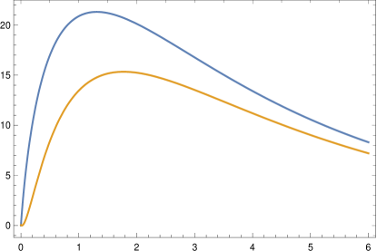
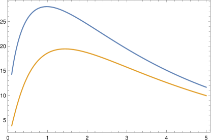
Figure 1: $<n_{k}>_{out}$ (along y axis) vs. $h_{0}$ (KR field energy density, along x axis). Left figure : for $\xi=1/6$ ; $k=0.01$, $m=0$ (upper figure) and $k=0.01$, $m=0.5$ (lower figure). Right figure : for $\xi=0$ ; $k=0.01$, $m=0$ (upper figure) and $k=0.01$, $m=0.5$ (lower figure).

The figures demonstrate the following informations:

• In the conformal coupling case : no particle production occurs for a massless scalar field in the absence of Kalb-Ramond field (i.e for $h_{0}=0$), however the presence of KR field (i.e $h_{0}\neq 0$) leads to a non-zero value of $<n_{k}>_{out}$ even for $m=0$. This is a consequence of the fact that the presence of the KR field breaks the conformal symmetry of the massless scalar field even for $\xi=1/6$ in four dimensional context, which is clearly evident from action (1). On the other hand, in the weak coupling case, $<n_{k}>_{out}$ is non-zero for all values of $h_{0}$ ($h_{0}\geq 0$), as expected.

• Irrespective of conformal or weak coupling, $<n_{k}>_{out}$ has a maximum at a certain value of $h_{0}$. However here we show that the class of symmetric bouncing scale factor (irrespective of any specific form) leads to a maxima of $<n_{k}>_{out}$ at a finite value of $h_{0}$. In order to explore this, following we determine the rate of change of $<n_{k}>_{out}$, with respect to $\alpha h_{0}$, in the limits - $\frac{\alpha h_{0}}{(k^{2}+m^{2})}\ll 1$ (i.e for low KR field energy density) and $\frac{\alpha h_{0}}{(k^{2}+m^{2})}\gg 1$ (i.e for large KR field energy density) respectively. Using eqn.(31), we obtain the explicit expression of $|\beta_{k}\big{|}^{2}$ for a symmetric universe, as follows:

  $$|\beta_{k}\big{|}^{2}=\frac{1}{4\omega_{k}^{2}}\bigg{[}I_{1}-I_{2}+I_{3}\bigg{]}^{2}$$ (43)

  where the quantities within the square paranthesis have the following expressions:

  $$I_{1} = 2m^{2}\int_{0}^{\infty}d\eta\cos{(2\omega\eta)}\big{[}a^{2}(\infty)-a^{2}(\eta)\big{]}$$

  $$I_{2} = 2(\xi-1/6)\int_{0}^{\infty}d\eta\cos{(2\omega\eta)}R(\eta)a^{2}(\eta)$$

  $$I_{3} = 2\alpha h_{0}\int_{0}^{\infty}d\eta\cos{(2\omega\eta)}\bigg{[}\frac{1}{a^{4}(\infty)}-\frac{1}{a^{4}(\eta)}\bigg{]}$$ (44)

  Due to the condition $a(\eta)=a(-\eta)$ (for which the curvature $R(\eta)=6\ddot{a}/a^{3}$ also becomes symmetric), the integration limit in $I_{1}$, $I_{2}$ and $I_{3}$ becomes zero to infinity and the other integrals involving $\sin{(2\omega\eta)}$ vanish. Now in the expanding regime i.e for $0\leq\eta<\infty$, the quantity $\bigg{[}\frac{1}{a^{4}(\infty)}-\frac{1}{a^{4}(\eta)}\bigg{]}$ is negative and goes to zero asymptotically. Thereby the magnitude $\bigg{|}\frac{1}{a^{4}(\infty)}-\frac{1}{a^{4}(\eta)}\bigg{|}$ acquires the maximum value at $\eta=0$ and decreases monotonically with the expansion of our universe. On the other hand, $\cos{(2\omega\eta)}$ starts with a positive value from $\eta=0$. Thus the negative contribution of the integrand in $I_{3}$ exceeds than that of the positive contribution. As a consequence the integral $I_{3}$ must be a negative quantity. Similar argument leads to $I_{1}>0$ and $I_{2}\leq 0$ (the equality sign is for the conformal coupling). These informations will be useful later. With the help of eqn.(43), we determine the rate of change of $|\beta_{k}\big{|}^{2}$ (with respect to $\alpha h_{0}$) for two different regimes as follows:
  

  In the regime $\frac{\alpha h_{0}}{(k^{2}+m^{2})}\ll 1$, we get

  $$\frac{d\big{|}\beta_{k}\big{|}^{2}}{d(\alpha h_{0})} = -\frac{1}{(k^{2}+m^{2})}\int_{0}^{\infty}d\eta\cos{(2\omega\eta)}\bigg{[}\frac{1}{a^{4}(\infty)}-\frac{1}{a^{4}(\eta)}\bigg{]}$$ (45)

  $$\bigg{[} m^{2}\int_{0}^{\infty}d\eta\cos{(2\omega\eta)}\big{[}a^{2}(\infty)-a^{2}(\eta)\big{]}-(\xi-1/6)\int_{0}^{\infty}d\eta\cos{(2\omega\eta)}R(\eta)a^{2}(\eta)\bigg{]}>0,$$

  Thereby the particle number density increases with KR field energy density for small value of $\alpha h_{0}$. Similarly for $\frac{\alpha h_{0}}{(k^{2}+m^{2})}\gg 1$,

  $$\frac{d\big{|}\beta_{k}\big{|}^{2}}{d(\alpha h_{0})} = -\bigg{[}\int_{0}^{\infty}d\eta\cos{(2\omega\eta)}\bigg{(}\frac{1}{a^{4}(\infty)}-\frac{1}{a^{4}(\eta)}\bigg{)}\bigg{]}^{2}$$ (46)

  $$- 2\sqrt{\alpha h_{0}}\bigg{[}\int_{0}^{\infty}d\eta\cos{(2\omega\eta)}\bigg{(}\frac{1}{a^{4}(\infty)}-\frac{1}{a^{4}(\eta)}\bigg{)}\bigg{]}\bigg{[}\int_{0}^{\infty}d\eta~{}\eta\sin{(2\omega\eta)}\bigg{(}\frac{1}{a^{4}(\infty)}-\frac{1}{a^{4}(\eta)}\bigg{)}\bigg{]}<0,$$

  which indicates that $<n_{k}>_{out}$ decreases with KR field energy density for large $\alpha h_{0}$.
  Thus as a whole, $<n_{k}>_{out}$ ($=\big{|}\beta_{k}\big{|}^{2}$) increases with $h_{0}$ for $\frac{\alpha h_{0}}{(k^{2}+m^{2})}\ll 1$ while it decreases in the regime $\frac{\alpha h_{0}}{(k^{2}+m^{2})}\gg 1$. This entails that $<n_{k}>_{out}$ must has a maximum in between these two limits of $h_{0}$ in a symmetric bounce universe, which is also reflected through Figure[1] as the particular form of the scale factor we consider in eqn.(18) actually corresponds to a non-singular symmetric bounce. For $\frac{\alpha h_{0}}{(k^{2}+m^{2})}\ll 1$, the energy of the scalar particle can be approximated as $\omega_{k}\simeq\sqrt{k^{2}+m^{2}}$ i.e independent of $h_{0}$. Now due to the coupling $f(\Phi)$, the energy supplied from the KR field to the scalar field increases with increasing $h_{0}$. This along with the fact that the energy of each scalar particle is independent of $h_{0}$ explains why the particle production is enhanced as the KR field energy density increases for $\frac{\alpha h_{0}}{(k^{2}+m^{2})}\ll 1$. On the other hand, for $\frac{\alpha h_{0}}{(k^{2}+m^{2})}\gg 1$, the energy of scalar particle is proportional to $h_{0}$, in particular $\omega_{k}\propto\sqrt{h_{0}}$. Therefore it becomes more difficult to excite the scalar particle and consequently the particle production decreases with increasing $h_{0}$ for $\frac{\alpha h_{0}}{(k^{2}+m^{2})}\gg 1$. These explain the inequalities obtained in eqns.(45) and (46) respectively.

III.4 Quantum entanglement between scalar particles

The ”in“ and ”out“ eigenstates of the scalar field Hamiltonian can serve as two different basis sets in the Fock space and thus the field state can be expressed by two ways: either by in-eigenstates or by out-eigenstates i.e

$$|state~{}\textgreater=|0_{in}\textgreater=\sum c_{n}|n~{}\textgreater_{\vec{k}}^{out}|n~{}\textgreater_{-\vec{k}}^{out}$$ (47)

where $|0_{in}\textgreater$ and $|n~{}\textgreater_{\vec{k}}^{out}|n~{}\textgreater_{-\vec{k}}^{out}$ belong from the same Fock space and also $c_{n}$ denote the corresponding coefficients between these two states. Since we are working in the Heisenberg picture, the field state is taken as independent of time. Recall, the scalar field Hamiltonian density explicitly depends on time, not space (see eqn.(16)), which confirms that the energy of the scalar field is not a conserved quantity, but the three momentum is. This is clearly reflected through the above expression. However eqn.(47) further indicates that the field state is not separable with respect to out modes, which tells that the out modes get quantum entangled to each other. Such entanglement may be quantified by von-Neumann entropy ($S$) defined through the conception of reduced density operator as follows:

$$S=-Tr\bigg{[}\hat{\rho}_{\vec{k}}^{red}~{}\log_{2}(\hat{\rho}_{\vec{k}}^{red})\bigg{]}$$ (48)

in $k_{B}=1$ (Boltzmann constant) unit, where $\hat{\rho}_{\vec{k}}^{red}$ is the reduced density operator for $\vec{k}$th out modes and has the following definition

$$\hat{\rho}_{\vec{k}}^{red}=\sum\textless~{}m|~{}\hat{\rho}~{}|m~{}\textgreater_{\vec{-k}}^{out}$$ (49)

with $\hat{\rho}$ be the full density operator of the scalar field and given by

$$\hat{\rho}=|state~{}\textgreater\textless~{}state|=|0_{in}\textgreater\textless~{}0_{in}|$$ (50)

Going through the calculations shown in Appendix, one obtains the von-Neumann entropy in terms of Bogolyubov coefficients as follows:

$$S=\log_{2}\bigg{[}\frac{\gamma^{\gamma/(\gamma-1)}}{(1-\gamma)}\bigg{]}$$ (51)

with $\gamma=\bigg{|}\frac{\beta_{k}}{\alpha_{k}}\bigg{|}^{2}$ and the expressions of $|\alpha_{k}|^{2}$, $|\beta_{k}|^{2}$ are given in eqns.(38), (39) respectively.
To understand the effects of the KR field on cosmological entanglement entropy, we give the following plots : (1) Left part of Figure[2] is the variation of entropy ($S$) with respect to mass ($m$) of the scalar field for $\xi=1/6$ (i.e for conformal coupling) in absence of KR field, (2) Right part of Figure[2] is the 3D plot exploring the variation of $S$ with respect to mass ($0\leq m\leq 1$ along x axis, in Planckian unit) and KR field energy density ($0\leq h_{0}\leq 0.7$ along y axis, in Planckian unit) for $\xi=1/6$, (3) Left and right parts of Figure[3] give the same plots respectively for $\xi=0$ i.e for weak coupling case.

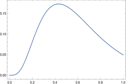
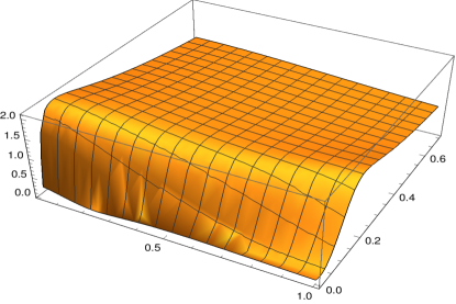
Figure 2: $Left~{}part$ : $S$ (along y axis) vs. $m$ (along x axis) for $\xi=1/6$ ; $k=0.01$ in absence of KR field. $Right~{}part$ : 3D plot of $S$ with respect to mass ($0\leq m\leq 1$ along x axis, in Planckian unit) and KR field energy density ($0\leq h_{0}\leq 0.7$ along y axis for $\xi=1/6$ ; $k=0.01$.

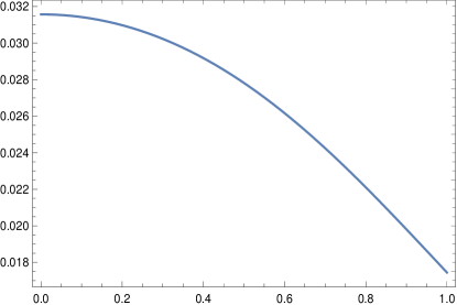
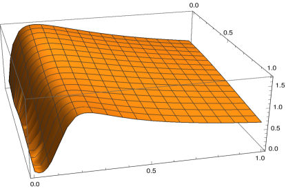
Figure 3: $Left~{}part$ : $S$ (along y axis) vs. $m$ (along x axis) for $\xi=0$ ; $k=0.01$ in absence of KR field. $Right~{}part$ : 3D plot of $S$ with respect to mass ($0\leq m\leq 1$ along x axis, in Planckian unit) and KR field energy density ($0\leq h_{0}\leq 0.7$ along y axis for $\xi=0$ ; $k=0.01$.

Figure[2] clearly demonstrates that in the case of conformal coupling and without the KR field, the entanglement entropy is bounded by $S\lesssim 0.17$ (in $k_{B}=1$, see the left part), while in presence of KR field the upper bound of entropy goes beyond $0.17k_{B}$ and reach up to $S\lesssim 2k_{B}$ (see the right part). Therefore if the entanglement entropy is found to lie within $0.17k_{B}\lesssim S\lesssim 2k_{B}$, then it may provide a possible testbed for the existence of Kalb-Ramond field in our universe. Similarly Figure[3] reveals that for $\xi=0$, if the von-Neumann entropy situates in between $0.032k_{B}$ and $1.5k_{B}$, then one can infer about the possible presence of KR field. Moreover it may be noticed from Fig.[2] that the presence of KR field causes a non-zero value of entropy even for $m=0$ and $\xi=1/6$ in four dimensional context. However this is one of the consequences of the fact that the presence of KR field breaks the conformal symmetry of a massless scalar field propagating in a four dimensional FRW spacetime (as mentioned earlier).
Thus it is clear that our argument regarding the testbed of Kalb-Ramond field through cosmological von-Neumann entropy relies on the fact that the entanglement entropy has a maxima at a finite value of $h_{0}$. However in the present paper we show such ”maximum“ character of entropy, but for a specific form of the scale factor considered in eqn.(18). Therefore it is important to investigate whether the von-Neumann entropy, in presence of KR field, possesses a maxima for a general class of scale factor. We investigate this in a bouncing universe, by determining the rate of change of $S$ with respect to $\alpha h_{0}$ in the regimes $\frac{\alpha h_{0}}{(k^{2}+m^{2})}\ll 1$ (i.e for low KR field energy density) and $\frac{\alpha h_{0}}{(k^{2}+m^{2})}\gg 1$ (i.e for large KR field energy density) respectively. Using eqn.(30), we determine the expression of $\big{|}\alpha_{k}\big{|}^{2}$ for the class of symmetric bouncing scale factor as follows,

$$\big{|}\alpha_{k}\big{|}^{2}=1+\bigg{[}J_{1}-J_{2}+J_{3}\bigg{]}^{2}$$ (52)

where the $J_{i}$ ($i=1,2,3$) have the following expressions:

$$J_{1} = m^{2}\int_{-\infty}^{\infty}d\eta\big{[}a^{2}(\infty)-a^{2}(\eta)\big{]}$$

$$J_{2} = (\xi-1/6)\int_{-\infty}^{\infty}d\eta R(\eta)a^{2}(\eta)$$

$$J_{3} = \alpha h_{0}\int_{-\infty}^{\infty}d\eta\bigg{[}\frac{1}{a^{4}(\infty)}-\frac{1}{a^{4}(\eta)}\bigg{]}$$ (53)

Due to the fact $a(\eta)\leq a(\infty)$, the above integrals satisfy the inequalities as $J_{1}>0$, $J_{2}\leq 0$ (recall we are interested on the weak coupling and the conformal coupling cases i.e $\xi=0$ and $\xi=1/6$ respectively. For $\xi=0$, $J_{2}$ becomes negative, while for $\xi=1/6$, $J_{2}$ becomes zero; that is why, as a whole we consider $J_{2}\leq 0$ where the equality sign is for the conformal coupling) and $J_{3}<0$. Using these expressions, we obtain $\frac{d\big{|}\alpha_{k}\big{|}^{2}}{d(\alpha h_{0})}$ in the limit $\frac{\alpha h_{0}}{(k^{2}+m^{2})}\ll 1$ as follows:

$$\frac{d\big{|}\alpha_{k}\big{|}^{2}}{d(\alpha h_{0})} = \frac{1}{2(k^{2}+m^{2})}\int_{-\infty}^{\infty}d\eta\bigg{(}\frac{1}{a^{4}(\infty)}-\frac{1}{a^{4}(\eta)}\bigg{)}$$ (54)

$$\bigg{[} m^{2}\int_{-\infty}^{\infty}d\eta\big{[}a^{2}(\infty)-a^{2}(\eta)\big{]}-(\xi-1/6)\int_{-\infty}^{\infty}d\eta R(\eta)a^{2}(\eta)\bigg{]}<0$$

The first integral in the R.H.S of eqn.(54) is negative while the quantity within the square braket is positive, this results that $\big{|}\alpha_{k}\big{|}^{2}$ decreases with $\alpha h_{0}$ for small value of $\frac{\alpha h_{0}}{k^{2}+m^{2}}$. Similarly in the regime $\frac{\alpha h_{0}}{(k^{2}+m^{2})}\gg 1$ we get,

$$\frac{d\big{|}\alpha_{k}\big{|}^{2}}{d(\alpha h_{0})}=\frac{1}{4}\bigg{[}\int_{-\infty}^{\infty}d\eta\bigg{(}\frac{1}{a^{4}(\infty)}-\frac{1}{a^{4}(\eta)}\bigg{)}\bigg{]}^{2}>0$$ (55)

The expression $\gamma=\bigg{|}\frac{\beta_{k}}{\alpha_{k}}\bigg{|}^{2}$ leads to the variation of $\gamma$ with the KR field energy density as follows:

$$\frac{d\gamma}{d(\alpha h_{0})}=\bigg{|}\frac{\beta_{k}}{\alpha_{k}}\bigg{|}^{2}\bigg{[}\frac{1}{\big{|}\beta_{k}\big{|}^{2}}\frac{d\big{|}\beta_{k}\big{|}^{2}}{d(\alpha h_{0})}-\frac{1}{\big{|}\alpha_{k}\big{|}^{2}}\frac{d\big{|}\alpha_{k}\big{|}^{2}}{d(\alpha h_{0})}$$ (56)

Having the above expression in hand along with the help of eqns.(45), (46), (54), (55), we can argue that $\frac{d\gamma}{d(\alpha h_{0})}$ takes positive and negative values in the limits $\frac{\alpha h_{0}}{(k^{2}+m^{2})}\ll 1$ and $\frac{\alpha h_{0}}{(k^{2}+m^{2})}\gg 1$ respectively. Therefore the quantity $\gamma$ must has a maxima at a finite value of $h_{0}$ in between these two limits. Eqn.(51) reveals that the entropy ($S$) is a monotonic increasing function of $\gamma$ by which we can argue that the von-Neumann entropy also possesses a maxima at a finite value of $h_{0}$. Hence the ”maximum“ character of cosmological entanglement entropy is not only confined within the scale factor as considered in eqn.(18) but also valid for a general class of the scale factor which corresponds to a symmetric bounce universe.

Before concluding, we would like to mention that the present investigation on cosmological entanglement in presence of Kalb-Ramond (KR) field can be extended to higher dimensions (see risi ; lahanas ; tuan1 ; tuan2 ; ssg_prl for some interesting papers working on high dimensional scenarios of the Kalb-Ramond theory). In higher dimensional picture, for example, in a five dimensional braneworld scenario (two brane model), the Kalb-Ramond field is generally considered to propagate in the five dimensional bulk. Moreover on projecting the bulk gravity on the brane, the extra dimensional modulus field appears as a scalar field (known as radion field) in the four dimensional effective theory of our visible brane GW . Thereby in the on-brane effective theory, the radion field gets coupled to the KR field tp1 . Thus the coupling between the scalar field and the KR field appears naturally in the five dimensional braneworld scenario, unlike to the case of four dimensional model where the scalar field has to be taken by hand (as we have considered the scalar field $\Phi$ in the action (1)). It seems that the investigation of cosmological entanglement in presence of KR field will be interesting and is expected to be studied in near future.

IV Conclusion

In the present paper, we deal with quantum evolution of a massive scalar field propagating in a four dimensional FRW spacetime where the scalar field has a non-minimal coupling with the Ricci scalar. The scalar field is also coupled with a second rank antisymmetric tensor field known as Kalb-Ramond (KR) field. In such a scenario, we try to address the possible effects of KR field on scalar particle production and quantum entanglement between the produced particles with a hope that the entanglement entropy may provide a possible testbed for the existence of the KR field in our universe. For this purpose, the spacetime and the KR field are considered as classical fields while the scalar field is treated as a quantum one. The classical evolution of KR field energy density is found to decrease with the cosmological expansion of our universe as $1/a^{6}$ (with $a$ being the scale factor) i.e with a faster rate in comparison to radiation ($\propto 1/a^{4}$) and matter ($\propto 1/a^{3}$) energy density. With this classical evolution, the possible effects of KR field are as follows :

1. In the absence of KR field, a massless scalar field possesses conformal symmetry for $\xi=1/6$ in four dimensional context. As a consequence, there occurs no particle production and the entanglement entropy vanishes for $m=0$ and $\xi=1/6$ in a background FRW spacetime. However the presence of KR field (actually the coupling between scalar and KR field) spoils such conformal symmetry, which in turn causes a definite particle production and also a non-zero value of entanglement entropy even for $m=0$, $\xi=1/6$ in a 4D FRW spacetime. These may be noticed from the Figures[1,2,3].

2. The interaction between the scalar field and the background time dependent gravitational field (i.e FRW spacetime) makes the scalar field Hamiltonian explicitly time dependent which in turn excites a certain number of scalar particles ($<n_{k}>_{out}$) in the ”out-region“ from an infinite-past-vacuum-state. Needless to say, $<n_{k}>_{out}$ depends on KR field energy density $h_{0}$ and also has a maximum at a finite value of $h_{0}$, irrespective of conformal or weak coupling, see Fig.[1]. The reason for acquiring such a maxima is that for $\frac{\alpha h_{0}}{(k^{2}+m^{2})}\ll 1$, the energy of the scalar particle can be approximated as $\omega_{k}\simeq\sqrt{k^{2}+m^{2}}$ i.e independent of $h_{0}$. Now due to the coupling $f(\Phi)$, the energy supplied from the KR field to the scalar field increases with increasing $h_{0}$. This along with the fact that the energy of each scalar particle is independent of $h_{0}$ explains why the particle production enhances as the KR field energy density increases for $\frac{\alpha h_{0}}{(k^{2}+m^{2})}\ll 1$. On the other hand, for $\frac{\alpha h_{0}}{(k^{2}+m^{2})}\gg 1$, the energy of scalar particle is proportional to $\sqrt{h_{0}}$, in particular $\omega_{k}\propto\sqrt{h_{0}}$. Therefore it becomes more difficult to excite the scalar particle and consequently the particle production decreases with increasing $h_{0}$ for $\frac{\alpha h_{0}}{(k^{2}+m^{2})}\gg 1$. Thus as a whole, $\frac{d<n_{k}>_{out}}{d(\alpha h_{0})}>0$ for $\frac{\alpha h_{0}}{(k^{2}+m^{2})}\ll 1$ while we get $\frac{d<n_{k}>_{out}}{d(\alpha h_{0})}<0$ in the regime $\frac{\alpha h_{0}}{(k^{2}+m^{2})}\gg 1$, which entails that $<n_{k}>_{out}$ must has a maximum in between these two limits.

3. The scalar field evolves from an asymptotic past vacuum state to a quantum entangled state with respect to ”out-modes“. The entanglement is quantified by von-Neumann entropy ($S$) in the present context. For a non-singular symmetric universe, irrespective of conformal and weak coupling case, we get $max[S(k,m,h_{0}\neq 0)]>max[S(k,m,h_{0}=0)]$ i.e the presence of KR field makes the upper bound of the entropy larger in comparison to the case when the KR field is absent. Therefore if the entanglement entropy is found to lie within these two upper bounds ( i.e within $max[S(k,m,h_{0}\neq 0)]$ and $max[S(k,m,h_{0}=0)]$ ), then it may provide a possible testbed for the existence of Kalb-Ramond field in our universe.
   

   Thereby the presence of KR field in a FRW bouncing universe allows a greater particle production and consequently the upper bound of the entanglement entropy becomes larger in comparison to the case when the KR field is absent. This in turn may provide a possible testbed for the existence of Kalb-Ramond field. However the measurement procedure of the entanglement entropy is still a problem. If the actual method of measurement of entanglement entropy in a cosmological background takes a shape in future, these predictions will certainly be useful to test the existence of a Kalb-Rammond field.

V Appendix: Detailed calculations of von-Neumann entropy

The in-vacuum can be expressed as linear combination of out-states as $|0_{in}\textgreater=\sum c_{n}|n~{}\textgreater_{\vec{k}}^{out}|n~{}\textgreater_{-\vec{k}}^{out}$. The coefficients $c_{n}$ play the most crucial role in determining the entanglement entropy.

V.1 Determination of $c_{n}$

As mentioned earlier, the in-vacuum is annihilated by $\hat{a}_{\vec{k}}$ i.e $\hat{a}_{\vec{k}}|0_{in}\textgreater=0$. Using Bogolyubov coefficients, one can write this annihilation condition as follows:

$$\big{(}\alpha_{k}^{*}\hat{b}_{\vec{k}}-\beta_{k}^{*}\hat{b}_{-\vec{k}}^{+}\big{)}|0_{in}\textgreater = 0$$

$$\Rightarrow\big{(}\alpha_{k}^{*}\hat{b}_{\vec{k}}-\beta_{k}^{*}\hat{b}_{-\vec{k}}^{+}\big{)}\sum c_{n}|n~{}\textgreater_{\vec{k}}^{out}|n~{}\textgreater_{-\vec{k}}^{out} = 0$$

$$\Rightarrow\sum c_{n}\alpha_{k}^{*}|n-1~{}\textgreater_{\vec{k}}^{out}|n~{}\textgreater_{-\vec{k}}^{out} = \sum c_{n}\beta_{k}^{*}|n~{}\textgreater_{\vec{k}}^{out}|n+1~{}\textgreater_{-\vec{k}}^{out}$$

$$\Rightarrow\alpha_{k}^{*}\sum c_{m+1}|m~{}\textgreater_{\vec{k}}^{out}|m+1~{}\textgreater_{-\vec{k}}^{out} = \beta_{k}^{*}\sum c_{n}|n~{}\textgreater_{\vec{k}}^{out}|n+1~{}\textgreater_{-\vec{k}}^{out}$$ (57)

Eqn.(57) clearly gives the recursion relation of the coefficients as

$$c_{1} = \frac{\beta_{k}^{*}}{\alpha_{k}^{*}}c_{0}$$

$$c_{2} = \frac{\beta_{k}^{*}}{\alpha_{k}^{*}}c_{1}=\bigg{(}\frac{\beta_{k}^{*}}{\alpha_{k}^{*}}\bigg{)}^{2}c_{0}$$

$$c_{n} = \frac{\beta_{k}^{*}}{\alpha_{k}^{*}}c_{n-1}=\bigg{(}\frac{\beta_{k}^{*}}{\alpha_{k}^{*}}\bigg{)}^{2}c_{n-2}=...........=\bigg{(}\frac{\beta_{k}^{*}}{\alpha_{k}^{*}}\bigg{)}^{n}c_{0}$$ (58)

Therefore all the coefficients $c_{n}$ ($n\geq 1$) depend on the single one $c_{0}$ which can be determined from the normalization condition of $|0_{in}\textgreater$ as follows:

$$\textless~{}0_{in}|0_{in}~{}\textgreater = 1$$

$$\Rightarrow\sum|c_{n}|^{2} = 1$$

$$\Rightarrow|c_{0}|^{2}\bigg{(}1+\bigg{|}\frac{\beta_{k}^{*}}{\alpha_{k}^{*}}\bigg{|}^{2}+\bigg{|}\frac{\beta_{k}^{*}}{\alpha_{k}^{*}}\bigg{|}^{4}+.......\bigg{)} = 1$$

$$\Rightarrow|c_{0}|^{2}\bigg{(}\frac{1}{1-\bigg{|}\frac{\beta_{k}^{*}}{\alpha_{k}^{*}}\bigg{|}^{2}}\bigg{)} = 1\Rightarrow|c_{0}|=\sqrt{1-\bigg{|}\frac{\beta_{k}^{*}}{\alpha_{k}^{*}}\bigg{|}^{2}}=\sqrt{1-\gamma}$$ (59)

where $\gamma=\bigg{|}\frac{\beta_{k}^{*}}{\alpha_{k}^{*}}\bigg{|}^{2}$. Thus eqns.(58) and (59) lead to the coefficient $c_{n}$ (in terms of Bogolyubov coefficients) as

$$c_{n}=\bigg{(}\frac{\beta_{k}^{*}}{\alpha_{k}^{*}}\bigg{)}^{n}\sqrt{1-\gamma}$$ (60)

from which the in-vacuum can be expressed (in terms of out-states) as,

$$|0_{in}\textgreater=\sum\bigg{(}\frac{\beta_{k}^{*}}{\alpha_{k}^{*}}\bigg{)}^{n}\sqrt{1-\gamma}|n~{}\textgreater_{\vec{k}}^{out}|n~{}\textgreater_{-\vec{k}}^{out}$$ (61)

V.2 Determination of von-Neumann entropy

The full density operator of the system is given by,

$$\hat{\rho} = |0_{in}\textgreater\textless~{}0_{in}|$$ (62)

$$= \sum_{n}\sum_{r}c_{n}c_{r}^{*}|n~{}\textgreater_{-\vec{k}}~{}|n~{}\textgreater_{\vec{k}}~{}\textless~{}r_{\vec{k}}|~{}\textless~{}r_{-\vec{k}}|$$

where we use the expansion of $|0_{in}\textgreater$ in terms of out-states. With the help of eqn.(62), we determine the reduced density operator as follows :

$$\hat{\rho}_{\vec{k}}^{red} = \sum_{m}\textless~{}m_{-\vec{k}}|\hat{\rho}|m_{-\vec{k}}~{}\textgreater$$ (63)

$$= \sum_{m}\sum_{n}\sum_{r}c_{n}c_{r}^{*}\textless~{}m|n~{}\textgreater~{}|n~{}\textgreater_{\vec{k}}~{}\textless~{}r_{\vec{k}}|\textless~{}r|m~{}\textgreater$$

$$= \sum_{m}\sum_{n}\sum_{r}c_{n}c_{r}^{*}|n~{}\textgreater_{\vec{k}}~{}\textless~{}r_{\vec{k}}|\delta_{mn}\delta_{mr}$$

$$= \sum_{n}\sum_{r}c_{n}c_{r}^{*}|n~{}\textgreater_{\vec{k}}~{}\textless~{}r_{\vec{k}}|\delta_{nr}$$

$$= \sum_{n}|c_{n}|^{2}|n~{}\textgreater_{\vec{k}}~{}\textless~{}n_{\vec{k}}|$$

The entanglement entropy between the out modes is measured by von-Neumann entropy defined by,

$$S = -Tr\bigg{[}\hat{\rho}_{\vec{k}}^{red}~{}\log_{2}(\hat{\rho}_{\vec{k}}^{red})\bigg{]}$$ (64)

$$= -\sum_{m}\textless~{}m_{\vec{k}}|\hat{\rho}_{\vec{k}}^{red}~{}\log_{2}(\hat{\rho}_{\vec{k}}^{red})|m_{\vec{k}}~{}\textgreater$$

Using eqn.(63), the above expression of $S$ can be simplified as follows :

$$S = -\sum_{m}\textless~{}m_{\vec{k}}|\hat{\rho}_{\vec{k}}^{red}~{}\log_{2}(\hat{\rho}_{\vec{k}}^{red})|m_{\vec{k}}~{}\textgreater$$ (65)

$$= -\sum_{n}|c_{n}|^{2}\bigg{(}\log_{2}|c_{n}|^{2}\bigg{)}=-|c_{0}|^{2}\sum_{n}\gamma^{n}\log_{2}\bigg{(}\gamma^{n}|c_{0}|^{2}\bigg{)}$$

$$= -|c_{0}|^{2}\bigg{[}\log_{2}\gamma\sum_{n}n\gamma^{n}+\log_{2}|c_{0}|^{2}\sum_{n}\gamma^{n}\bigg{]}$$

$$= \frac{\gamma}{\gamma-1}\log_{2}\gamma-\log_{2}\big{(}1-\gamma\big{)}=\log_{2}\bigg{[}\frac{\gamma^{\gamma/(\gamma-1)}}{(1-\gamma)}\bigg{]}$$

where we use $|c_{0}|^{2}=(1-\gamma)$, see eqn.(59). Eqn.(65) is the final expression of von-Neumann entropy in terms of Bogolyubov coefficients.

References

• (1) A. H. Guth, Phys. Rev. D 23 (1981) 347. doi:10.1103/PhysRevD.23.347.
• (2) A. A. Starobinsky, Phys. Lett. B 91 (1980) 99 [Phys. Lett. 91B (1980) 99] [Adv. Ser. Astrophys. Cosmol. 3 (1987) 130]. doi:10.1016/0370-2693(80)90670-X.
• (3) A. D. Linde, Phys. Lett. 129B (1983) 177. doi:10.1016/0370-2693(83)90837-7.
• (4) A. D. Linde, Lect. Notes Phys. 738 (2008) 1 [arXiv:0705.0164 [hep-th]].
• (5) D. S. Gorbunov and V. A. Rubakov, “Introduction to the theory of the early universe: Cosmological perturbations and inflationary theory,” Hackensack, USA: World Scientific (2011) 489 p.
• (6) D. H. Lyth and A. Riotto, Phys. Rept. 314 (1999) 1 [hep-ph/9807278].
• (7) R. Brandenberger and P. Peter, Found. Phys. 47 (2017) no.6, 797 doi:10.1007/s10701-016-0057-0 [arXiv:1603.05834 [hep-th]].
J. de Haro and Y. F. Cai, Gen. Rel. Grav. 47 (2015) no.8, 95 doi:10.1007/s10714-015-1936-y [arXiv:1502.03230 [gr-qc]].
Y. F. Cai, Sci. China Phys. Mech. Astron. 57 (2014) 1414 doi:10.1007/s11433-014-5512-3 [arXiv:1405.1369 [hep-th]].
S.D. Odintsov, V.K. Oikonomou ; Int.J.Mod.Phys. D26 (2017) no.08, 1750085.
S.D. Odintsov, V.K. Oikonomou ; Phys.Rev. D92 (2015) no.2, 024016.
S.D. Odintsov, V.K. Oikonomou ; Phys.Rev. D91 (2015) no.6, 064036.
A. Das, D. Maity, T. Paul, S. SenGupta ; Eur.Phys.J. C77 (2017) no.12, 813.
E. Elizalde, S.D. Odintsov, V.K. Oikonomou and T. Paul ; Nucl. Phys. B 954 (2020) 114984.
• (8) Y. Akrami et al. [Planck Collaboration], arXiv:1807.06211 [astro-ph.CO].
• (9) A. G. R. et al., “Observational Evidence from Supernovae for an Accelerating Universe and a Cosmological Constant,” The Astronomical Journal 116, 1009 (1998).
• (10) S. P. et al., “Measurements of and from 42 High-Redshift Supernovae,” The Astrophysical Journal 517, 565 (1999).
• (11) G. Aad and B. A. et al., “Search for squarks and gluinos using final states with jets and missing transverse momentum with the ATLAS detector in proton–proton collisions,” Physics Letters B 701, 186 (2011).
• (12) G. e. a. Aad, “Search for Supersymmetry Using Final States with One Lepton, Jets, and Missing Transverse Momentum with the ATLAS Detector in $\sqrt{s}=7$ TeV pp Collisions,” Phys. Rev. Lett. 106, 131802 (2011).
• (13) V. K. et al., “Search for supersymmetry in pp collisions at 7 TeV in events with jets and missing transverse energy,” Physics Letters B 698, 196 (2011).
• (14) V. K. et al., “Search for microscopic black hole signatures at the Large Hadron Collider,” Physics Letters B 697, 434 (2011).
• (15) N. D. Birrell and P. C. W. Davies, Quantum Field Thoery in Curved Space (Cambridge, 1982).
• (16) J. L. Ball, I. Fuentes-Schuller, and F. P. Schuller, “Entanglement in an expanding spacetime,” Phys. Lett. A 359, 550 (2006).
• (17) I. Fuentes et al., “Entanglement of Dirac fields in an expanding spacetime,” Phys. Rev. D 82, 045030 (2010).
• (18) G. Ver Steeg and N. C. Menicucci, “Entangling Power of an Expanding Universe,” Phys. Rev. D 79, 044027 (2009).
• (19) M. Genovese, “Cosmology and Entanglement,” Advanced Science Letters 2, 303 (2009).
• (20) E. Martin-Martinez, Alexander R. H. Smith and Daniel R. Terno ; Phys.Rev. D93 (2016) no.4, 044001.
• (21) E. Martin-Martinez and N. C. Menicucci ; Class.Quant.Grav. 31 (2014) no.21, 214001.
• (22) E. Martin-Martinez and N. C. Menicucci ; Class.Quant.Grav. 29 (2012) 224003
• (23) S. Moradi, R. Pierini and S. Mancini ; Phys.Rev. D89 (2014) no.2, 024022.
• (24) R. Pierini, S. Moradi and S. Mancini ; Int.J.Theor.Phys. 55 (2016) no.6, 3059-3078.
• (25) R. Pierini, S. Moradi and S. Mancini ; Nucl.Phys. B924 (2017) 684-698.
• (26) Y. Nakai, N. Shibaa and M. Yamada ; arxiv: 1709.02390 [hep-th].
• (27) S. Mancini, R. Pierini and M. M. Wilde ; New J.Phys. 16 (2014) no.12, 123049.
• (28) M. Kalb and P. Ramond ; Phys. Rev. D 9 (1974) 2273.
• (29) C.G. Callan Jr., E.J. Martinec, M.J. Perry and D. Friedan ; Nucl. Phys. B 262 (1985) 593.
• (30) I. L. Buchbinder, E. N. Kirillova and N. G. Pletnev, Phys. Rev. D 78 (2008) 084024 doi:10.1103/PhysRevD.78.084024 [arXiv:0806.3505 [hep-th]].
• (31) P.S. Howe, A. Opfermann and G. Papadopoulos, hep-th/9710072.
• (32) P.S. Howe and G. Papadopoulos, Phys. Lett. B, 379 80 (1996).
• (33) A. Yu. Kubyshin, J. Math. Phys., 35 310 (1994).
• (34) G. German, A. Macias and O. Obregon, Class. Quantum Grav., 10 1045 (1993).
• (35) S. Kar, P. Majumdar, S. SenGupta and A. Sinha, Eur. Phys. J. C 23, 357 (2002).
• (36) S. Kar, P. Majumdar, S. SenGupta and S. Sur, Class. Quant. Grav. 19, 677 (2002).
• (37) P. Majumdar and S. SenGupta, Class. Quantum Grav. 16, L89 (1999).
• (38) E. Elizalde, S. D. Odintsov, T. Paul and D.S. Chillon Gomez ; Phys.Rev. D99 (2019) no.6, 063506.
• (39) E. Elizalde, S.D. Odintsov, V.K. Oikonomou and T. Paul ; JCAP 1902 (2019) 017.
• (40) T. Paul and S. SenGupta ; Eur. Phys. J. C 79 (2019) 7, 591.
• (41) G. De Risi ; Phys. Rev. D 77 (2008) 044030.
• (42) C. Chiou-Lahanas, G.A. Diamandis and B.C. Georgalas ; Phys.Lett.B 678: (2009) 485-490.
• (43) Tuan Q. Do and W. F. Kao ; Eur. Phys. J. C 78 (2018) 531.
• (44) Tuan Q. Do and W. F. Kao ; Phys. Rev. D 101 (2020) 044014.
• (45) B. Mukhopadhyaya, S. Sen, and S. SenGupta, Phys. Rev. Lett. 89, (2002) 121101.
• (46) W. D. Goldberger and M. B. Wise, Phys. Lett B 475 (2000) 275-279.