Equilibrium configuration of a rectangular obstacle immersed in a channel flow

Abstract.

Fluid flows around an obstacle generate vortices which, in turn, generate lift forces on the obstacle. Therefore, even in a perfectly symmetric framework equilibrium positions may be asymmetric. We show that this is not the case for a Poiseuille flow in an unbounded 2D channel, at least for small Reynolds number and flow rate. We consider both the cases of vertically moving obstacles and obstacles rotating around a fixed pin.

AMS Subject Classification: 35Q30, 35A02, 46E35, 31A15.

Keywords: viscous fluids, lift on an obstacle, stability.

1. Introduction and main result

We consider two different fluid-structure problems for a Poiseuille flow through an unbounded 2D channel containing an obstacle. In the first problem, a rigid rectangular body $B$ is immersed in an unbounded channel $\mathbb{R}\times(-L,L)$ and is free to move vertically under the action of both a fluid flow and of transverse restoring forces, as in Figure 1.

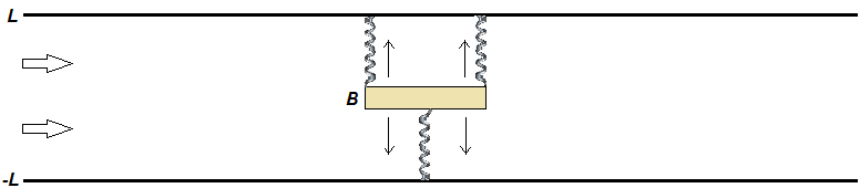
Figure 1. The channel with the vertically moving obstacle $B$.

In the second problem, the body $B$ is immersed in the same channel $\mathbb{R}\times(-L,L)$ but is only free to rotate around a pin located at its center of mass, see Figure 2.

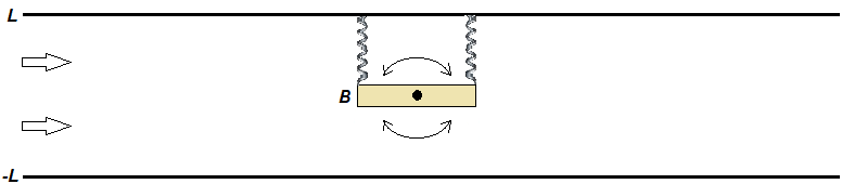
Figure 2. The channel with the rotating obstacle $B$.

These two problems are inspired to some bridge models considered in [2, 6]. The obstacle $B$ represents the cross-section of the deck of a suspension bridge, that may display both vertical and torsional oscillations, see [5]. Here we have decoupled these two motions and the action of the restoring forces that generate them.

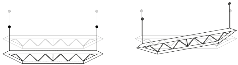
Figure 3. Vertical (left) and torsional (right) displacements of a deck.

The vertical oscillations in Figure 1 (and on the left of Figure 3) are created by three kinds of forces. There is an upwards restoring force due to the elastic action of both the hangers and the sustaining cables which, somehow, behave as linear springs which may slacken so that they have no downwards action. There is the weight of the deck which acts constantly downwards: this explains why there is no odd requirement on $f$ in (2). Finally, there is a resistance to both bending and stretching of the whole deck for which $B$ merely represents a cross-section: this force is superlinear and explains the infinite limit in (2), the deck is not allowed to go too far away from its equilibrium (horizontal) position due to the elastic resistance to deformations of the whole deck. The torsional oscillations are symmetric, they are due to the possible different behaviors of the hangers and cables at the two endpoints of the cross-section, see Figure 2 and the right picture in Figure 3. Their symmetric action translates into the odd assumption on $g$ in (6). Moreover, the restoring force of the hangers+cables system is not as violent and strong as the action of the whole deck, resisting to bending and stretching: this is why at the endpoints $g$ has a weaker behavior than $f$. The decoupling of vertical and torsional displacement, as well as the causes generating them, is a first step to understand the behavior of the deck under the action of the wind (assumed here to be governed by a Poiseuille flow). The full coupled vertical-torsional motion will be studied in a forthcoming paper.

For the first problem, a rigid rectangular body $B=[-d,d]\times[-\delta,\delta]$ is immersed in an unbounded channel $\mathbb{R}\times(-L,L)$ and is free to move vertically under the action of both a fluid flow and of transverse restoring forces. The union of the upper and lower boundaries of the channel is denoted by $\Gamma=\mathbb{R}\times\{-L,L\}$. The position of the center of mass of the body $B$ is indicated by $h$ and is counted from the middle line $x_{2}=0$ of the strip. The body $B$ may take different positions after translations in the vertical direction ${\mbox{\boldmath$e$}}_{2}$, namely,

$$B_{h}=B+h{\mbox{\boldmath$e$}}_{2}\qquad\forall|h|<L-\delta\,.$$

The cases $|h|=L-\delta$ correspond to a collision of the body $B$ with $\Gamma$. The domain occupied by the fluid then depends on $h$ and is denoted by

$$\Omega_{h}=\mathbb{R}\times(-L,L)\setminus B_{h},$$

see again Figure 1. The motion of the fluid is governed by the Navier-Stokes equations driven by a Poiseuille flow of prescribed flow rate.

We are interested in determining the equilibrium position of the body, for a given flow regime of the fluid. This leads us to determine the time-independent solutions to the following fluid-structure-interaction evolution problem (in dimensionless form)

(1) $$\begin{array}[]{cc}{\mbox{\boldmath$u$}}_{t}-\mbox{\rm div}{\mbox{\boldmath$T$}}({\mbox{\boldmath$u$}},p)+{\mathcal{R}}{\mbox{\boldmath$u$}}\cdot\nabla{\mbox{\boldmath$u$}}=0,\quad\mbox{\rm div}{\mbox{\boldmath$u$}}=0\quad\mbox{in $\Omega_{h}\times(0,T)$}\\ \vskip 6.0pt plus 2.0pt minus 2.0pt\vskip 3.0pt plus 1.0pt minus 1.0pt{\mbox{\boldmath$u$}}\left|\right._{\partial B_{h}}=\dot{h}{\mbox{\boldmath$e$}}_{2},\quad{\mbox{\boldmath$u$}}\left|\right._{\Gamma}=0,\quad{\displaystyle\lim_{\footnotesize|x_{1}|\to\infty}}{\mbox{\boldmath$u$}}(x_{1},x_{2})=\lambda(L^{2}-x_{2}^{2}){\mbox{\boldmath$e$}}_{1},\\ \ddot{h}+f(h)=-{\mbox{\boldmath$e$}}_{2}\cdot\int_{\partial B_{h}}{\mbox{\boldmath$T$}}({\mbox{\boldmath$u$}},p)\cdot{\mbox{\boldmath$n$}}\quad\mbox{in $(0,T)$\,.}\end{array}$$

Here $u$ and $p$ denote (non-dimensional) velocity and pressure fields of the fluid, whereas $n$ is the outward normal to $\partial\Omega_{h}$ so that, on $\partial B_{h}$, it is directed in the interior of $B_{h}$. Moreover, we use $\delta$ (the “thickness” of the body) as length scale, i.e. $\delta=1$ and set ${\mathcal{R}}=V/\nu$, $\lambda=|\Phi|/\nu$, where $V$ is a reference speed and $|\Phi|$ denotes the magnitude of the flow rate associated to the Poiseuille motion. For simplicity, for the rescaled $L$ and $d$ we maintain the same notation. We emphasize that $\Omega_{h}$ and $\partial B_{h}$ depend on $h$ through the position of $B_{h}$ so that the solution $u$ of (1) depends on $h$ as well; clearly, $u$ also depends on ${\mathcal{R}}$. The ODE (1)₃ states that the motion of the obstacle $B$ is driven by a nonlinear oscillator equation with elastic restoring force $f=f(h)$ (having the same sign as $h$), and forced by the fluid lift exerted on $B$. We assume that $f\in C^{1}(-L+1,L-1)$ satisfies

(2) $$f^{\prime}(h)>0\ \forall h\in(-L+1,L-1),\quad\lim_{|h|\to L-1}\ |f(h)|(|L-1|-|h|)^{\frac{3}{2}}=+\infty\,.$$

The last condition in (2) has the meaning of a strong force aiming to prevent collisions of $B$ with $\Gamma$: this means that the elastic spring is superlinear and has a limit extension before becoming plastic. This condition is necessary due to the boundary layer that forms when $B$ is close to $\Gamma$, with related appearance of large pressures.

Thus, by eliminating all time derivatives in (1), our objective reduces to find a solution $({\mbox{\boldmath$u$}},p,h)$ to the following boundary-value problem

(3) $$\begin{array}[]{cc}\mbox{\rm div}{\mbox{\boldmath$T$}}({\mbox{\boldmath$u$}},p)={\mathcal{R}}{\mbox{\boldmath$u$}}\cdot\nabla{\mbox{\boldmath$u$}},\quad\mbox{\rm div}{\mbox{\boldmath$u$}}=0\quad\mbox{in $\Omega_{h}$}\\ \vskip 6.0pt plus 2.0pt minus 2.0pt\vskip 3.0pt plus 1.0pt minus 1.0pt{\mbox{\boldmath$u$}}\left|\right._{\partial B_{h}}={\mbox{\boldmath$u$}}\left|\right._{\Gamma}=0,\quad{\displaystyle\lim_{\footnotesize|x_{1}|\to\infty}}{\mbox{\boldmath$u$}}(x_{1},x_{2})=\lambda(L^{2}-x_{2}^{2}){\mbox{\boldmath$e$}}_{1},\end{array}$$

subject to the compatibility condition

(4) $$f(h)=-{\mbox{\boldmath$e$}}_{2}\cdot\int_{\partial B_{h}}{\mbox{\boldmath$T$}}({\mbox{\boldmath$u$}},p)\cdot{\mbox{\boldmath$n$}}.$$

We emphasize that the lift is well defined in a generalized sense for weak solutions, see [6, Section 3.3].

In the second problem, we assume that the body $B$ is free to rotate around a pin located at its center of mass: this means that there is no obstruction for $B$ to reach a vertical position, which translates into the constraint that $L^{2}>1+d^{2}$ (the half diagonal of $B$ is less than the distance from the pin to $\Gamma$); see again Figure 2. The different positions of $B$ are now indexed with a parameter $\theta$ representing the angle of rotation with respect to the horizontal

$$B_{\theta}=\left(\begin{array}[]{lr}\cos\theta&-\sin\theta\\ \sin\theta&\cos\theta\end{array}\right)B\qquad\forall|\theta|<\frac{\pi}{2}.$$

The domain occupied by the fluid then depends on $\theta$ and is denoted by

$$\Omega_{\theta}=\mathbb{R}\times(-L,L)\setminus B_{\theta}.$$

We suppose that the body is subject to an angular restoring force $g=g(\theta)$ (a torque) and we are again interested in equilibrium positions which, in this case, are obtained by finding time-independent solutions to the following fluid-structure-interaction evolution problem

(5) $$\begin{array}[]{cc}\vskip 6.0pt plus 2.0pt minus 2.0pt\vskip 3.0pt plus 1.0pt minus 1.0pt{\mbox{\boldmath$u$}}_{t}-\mbox{\rm div}{\mbox{\boldmath$T$}}({\mbox{\boldmath$u$}},p)+{\mathcal{R}}{\mbox{\boldmath$u$}}\cdot\nabla{\mbox{\boldmath$u$}}=0,\quad\mbox{\rm div}{\mbox{\boldmath$u$}}=0\quad\mbox{in $\Omega_{\theta}\times(0,T)$}\\ \vskip 6.0pt plus 2.0pt minus 2.0pt{\mbox{\boldmath$u$}}\left|\right._{\partial B_{\theta}}=\dot{\theta}{\mbox{\boldmath$e$}}_{3}\times\mbox{\boldmath$x$},\quad{\mbox{\boldmath$u$}}\left|\right._{\Gamma}=0,\quad{\displaystyle\lim_{\footnotesize|x_{1}|\to\infty}}{\mbox{\boldmath$u$}}(x_{1},x_{2})=\lambda(L^{2}-x_{2}^{2}){\mbox{\boldmath$e$}}_{1},\\ \ddot{\theta}+g(\theta)={\mbox{\boldmath$e$}}_{3}\cdot\int_{\partial B_{\theta}}\mbox{\boldmath$x$}\times{\mbox{\boldmath$T$}}({\mbox{\boldmath$u$}},p)\cdot{\mbox{\boldmath$n$}}\quad\mbox{in $(0,T)$}\,.\end{array}$$

Besides the dissimilar geometry of the spatial domains, the other (formal) difference between (5) and (1) relies in the boundary condition over $\partial B$. We shall assume that $g\in C^{1}(-\frac{\pi}{2},\frac{\pi}{2})$ satisfies

(6) $$g\mbox{ odd},\quad g^{\prime}(\theta)>0\ \forall\theta\in\big{(}-\tfrac{\pi}{2},\tfrac{\pi}{2}\big{)},\quad\lim_{\theta\to\pi/2}\ g(\theta)=+\infty\,.$$

Compared to (2), we notice in (6) the additional oddness assumption and the weaker requirement at the extremal positions. We emphasize that the restriction to the interval $(-\frac{\pi}{2},\frac{\pi}{2})$ is due to physical reasons, since we have in mind the cross-section of the deck of a bridge which cannot reach a vertical position. From a purely mathematical point of view, the interval could be extended to $(-\pi,\pi)$ (allowing an upside down rotation) and even larger intervals giving the freedom of multiple rotations.

Also in this case, we look for time-independent (weak) solutions to (5), that is, solutions $({\mbox{\boldmath$u$}}(\theta,{\mathcal{R}}),\theta)\in H^{1}(\Omega_{\theta})\times(-\frac{\pi}{2},\frac{\pi}{2})$ satisfying the steady-state problem (3) (with $\Omega_{h}$ replaced by $\Omega_{\theta}$ and boundary values given in (5)) along with the compatibility condition

(7) $$g(\theta)={\mbox{\boldmath$e$}}_{3}\cdot\int_{\partial B_{\theta}}\mbox{\boldmath$x$}\times{\mbox{\boldmath$T$}}({\mbox{\boldmath$u$}},p)\cdot{\mbox{\boldmath$n$}}$$

Again, we emphasize that we can give a meaning to the torque for weak solutions, arguing as in [6, Section 3.3] for the lift.

Our main result, for both problems, states the uniqueness of the equilibrium position for small Reynolds numbers.

Theorem 1.

Assume that $f\in C^{1}(-L+1,L-1)$ and $g\in C^{1}(-\frac{\pi}{2},\frac{\pi}{2})$ satisfy (2) and (6). There exists ${\mathcal{R}}_{0}>0$ and $\lambda_{0}>0$ such that if ${\mathcal{R}}<{\mathcal{R}}_{0}$ and $\lambda<\lambda_{0}$ then:

$\bullet$ the problem (3)-(4) admits a unique solution $({\mbox{\boldmath$u$}}(h,{\mathcal{R}}),h)\in H^{1}(\Omega_{h})\times(-L+d,L-d)$ given by $({\mbox{\boldmath$u$}}(0,{\mathcal{R}}),0)$;

$\bullet$ the problem (3)-(7) admits a unique solution $({\mbox{\boldmath$u$}}(\theta,{\mathcal{R}}),\theta)\in H^{1}(\Omega_{\theta})\times(-\frac{\pi}{2},\frac{\pi}{2})$ given by $({\mbox{\boldmath$u$}}(0,{\mathcal{R}}),0)$.

For both problems, the solutions are smooth ($C^{\infty}(\Omega_{h})$ or $C^{\infty}(\Omega_{\theta})$) in the interior.

The proofs for the two problems (3)-(4) and (3)-(7) follow the same strategy, with some slight modifications. We give a sketch of the two proofs in Section 2.

2. Sketch of the proof of Theorem 1

We begin by showing well-posedness for (3) without imposing any fluid-structure constraint, neither (4), nor (7). As the condition at infinity is not homogeneous, we look for a solution written as

$${\mbox{\boldmath$u$}}={\mbox{\boldmath$v$}}+\lambda{\mbox{\boldmath$a$}},$$

where ${\mbox{\boldmath$v$}}\in H^{1}_{0}(\Omega_{h})$ and $a$ is a solenoidal vector field which is equal to $(L^{2}-x_{2}^{2}){\mbox{\boldmath$e$}}_{1}$ outside a compact set and vanishes on $\partial B$. We refer to [3, VI.1 and XIII] for more details on the functional setting. Since we seek an energy bound independent of the position of $B$, we introduce two specific extensions $a$ and $b$ of the Poiseuille flow which vanish on either $B_{h}$ or $B_{\theta}$. By the symmetry of the problem (3)-(4), one can assume that $B_{h}$ lies entirely above the horizontal line $x_{2}=-L+1+\tau$ where $\tau>0$ and $-L+1+\tau<0$. We then define $a$ as follows. Consider the domain

$$\Sigma=(-4d,-2d)\times(-L,L)\cup[-2d,2d]\times(-L,-L+1+\tau)\cup(2d,4d)\times(-L,L).$$

We also introduce

$$\Omega_{\infty}=\{(x_{1},x_{2});\,|x_{1}|\geq 4d,\ |x_{2}|\leq L\},\qquad\Omega_{d}=\{(x_{1},x_{2});\,|x_{1}|\leq 4d,\ (x_{1},x_{2})\in\Omega_{h}\}.$$

Let $\zeta$ be a cutoff function separating the obstacle and the Poiseuille flow at infinity, e.g.

$$\zeta(x_{1},x_{2})=\zeta(x_{1})=\left\{\begin{array}[]{ll}0&\mbox{ if }|x_{1}|<3d\\ 1&\mbox{ if }|x_{1}|>4d\end{array}\right.\qquad\zeta\in C^{\infty}\big{(}\mathbb{R}\times[-L,L]\big{)}.$$

Consider the problem

$$\mbox{\rm div}{\mbox{\boldmath$z$}}=\zeta^{\prime}(x_{1})(L^{2}-x_{2}^{2})\mbox{ in }\Sigma,\quad{\mbox{\boldmath$z$}}=0\mbox{ on }\partial\Sigma\,;$$

by [3, Theorem III.3.3] this problem admits a solution ${\mbox{\boldmath$z$}}\in H^{2}_{0}(\Sigma)$ because $\zeta^{\prime}(x_{1})(L^{2}-x_{2}^{2})\in H^{1}_{0}(\Sigma)$. Moreover, we have the estimate

$$\|\nabla{\mbox{\boldmath$z$}}\|_{H^{1}(\Sigma)}\leq c\|\zeta^{\prime}(x_{1})(L^{2}-x_{2}^{2})\|_{H^{1}(\Sigma)},$$

where $c>0$ depends only on $\Sigma$. Hence, if we extend $z$ by zero outside $\Sigma$ we obtain that ${\mbox{\boldmath$z$}}\in H^{1}_{0}(\mathbb{R}\times(-L,L))$. Then we define

$${\mbox{\boldmath$a$}}(\mbox{\boldmath$x$}):=\zeta(x_{1})(L^{2}-x_{2}^{2}){\mbox{\boldmath$e$}}_{1}-{\mbox{\boldmath$z$}}(\mbox{\boldmath$x$})$$

in such a way that $\mbox{\rm div}{\mbox{\boldmath$a$}}=0$. It is clear that ${\mbox{\boldmath$a$}}\in H^{2}_{loc}(\Omega_{h})$ and that ${\mbox{\boldmath$a$}}=(L^{2}-x_{2}^{2}){\mbox{\boldmath$e$}}_{1}$ for $|x_{1}|\geq 4d$. It follows that ${\mbox{\boldmath$a$}}\cdot\nabla{\mbox{\boldmath$a$}}=0$ for $|x_{1}|\geq 4d$ and $-\Delta{\mbox{\boldmath$a$}}=\nabla\Pi$ for $|x_{1}|\geq 4d$, where $\Pi(x_{1},x_{2})=2x_{1}$. We take as weak formulation of (3)

$$\int_{\Omega_{h}}\nabla{\mbox{\boldmath$v$}}:\nabla\mbox{\boldmath$\varphi$}={\mathcal{R}}\int_{\Omega_{h}}\Big{[}{\mbox{\boldmath$v$}}\cdot\nabla\mbox{\boldmath$\varphi$}+\lambda{\mbox{\boldmath$a$}}\cdot\nabla\mbox{\boldmath$\varphi$}\Big{]}{\mbox{\boldmath$v$}}-\lambda\int_{\Omega_{h}}\Big{[}{\mbox{\boldmath$v$}}\cdot\nabla{\mbox{\boldmath$a$}}+{\mbox{\boldmath$a$}}\cdot\nabla{\mbox{\boldmath$a$}}\big{]}\mbox{\boldmath$\varphi$}+\lambda\int_{\Omega_{h}}\Delta{\mbox{\boldmath$a$}}\cdot\mbox{\boldmath$\varphi$},$$

for any solenoidal test function $\mbox{\boldmath$\varphi$}\in\mathcal{D}(\Omega_{h})$. It is crucial to control the terms

$$\int_{\Omega_{h}}({\mbox{\boldmath$a$}}\cdot\nabla{\mbox{\boldmath$a$}})\mbox{\boldmath$\varphi$}=\int_{\Omega_{d}}({\mbox{\boldmath$a$}}\cdot\nabla{\mbox{\boldmath$a$}})\mbox{\boldmath$\varphi$}+\int_{\Omega_{\infty}}({\mbox{\boldmath$a$}}\cdot\nabla{\mbox{\boldmath$a$}})\mbox{\boldmath$\varphi$}$$

and

$$\int_{\Omega_{h}}\Delta{\mbox{\boldmath$a$}}\cdot\mbox{\boldmath$\varphi$}=\int_{\Omega_{d}}\Delta{\mbox{\boldmath$a$}}\cdot\mbox{\boldmath$\varphi$}+\int_{\Omega_{\infty}}\Delta{\mbox{\boldmath$a$}}\cdot\mbox{\boldmath$\varphi$}.$$

This can be clearly done since ${\mbox{\boldmath$a$}}\cdot\nabla{\mbox{\boldmath$a$}}=0$ in $\Omega_{\infty}$ and

$$\int_{\Omega_{\infty}}\Delta{\mbox{\boldmath$a$}}\cdot\mbox{\boldmath$\varphi$}=-\int_{\Omega_{\infty}}\nabla\Pi\cdot\mbox{\boldmath$\varphi$}=0.$$

When dealing with problem (3)-(7), we consider an open ball $\mathcal{B}$ in the channel $\mathbb{R}\times(-L,L)$ that contains $B_{\theta}$ for every $\theta\in[0,2\pi]$. Then we argue as in the previous case to construct ${\mbox{\boldmath$b$}}\in H^{2}_{loc}(\Omega_{h})$ such that ${\mbox{\boldmath$b$}}=(L^{2}-x_{2}^{2}){\mbox{\boldmath$e$}}_{1}$ for $|x_{1}|\geq 4d$ and ${\mbox{\boldmath$b$}}=0$ in $\mathcal{B}$.

Lemma 2.

There exists a constant $\gamma_{0}>0$ independent of $h\in(-L+1,L-1)$ and of $\theta\in(-\frac{\pi}{2},\frac{\pi}{2})$ such that if ${\mathcal{R}}\cdot\lambda<\gamma_{0}$, the problem (3) admits a weak solution ${\mbox{\boldmath$u$}}={\mbox{\boldmath$u$}}(h)$ (resp. ${\mbox{\boldmath$u$}}={\mbox{\boldmath$u$}}(\theta)$ when $\Omega_{h}$ is replaced by $\Omega_{\theta}$). Moreover, there exists $C=C(\mathcal{R},\lambda,L)>0$ (independent of $h$ and $\theta$), with $C\to 0$ as $(\mathcal{R},\lambda)\to 0$, such that

(8) $$\|\nabla\left({\mbox{\boldmath$u$}}-\lambda{\mbox{\boldmath$a$}}\right)\|_{2,\Omega_{h}}\leq C\qquad\forall\,h\in(-L+1,L-1),$$

(9) $$\mbox{resp. }\quad\|\nabla\left({\mbox{\boldmath$u$}}-\lambda{\mbox{\boldmath$b$}}\right)\|_{2,\Omega_{\theta}}\leq C\qquad\forall\,\theta\in\left(-\frac{\pi}{2},\frac{\pi}{2}\right).$$

This solution is also unique in the class of weak solutions, provided ${\mathcal{R}}\cdot\lambda$ and $\lambda$ are below a certain constant depending only on $L$. Moreover, ${\mbox{\boldmath$u$}}(h)$ (resp. ${\mbox{\boldmath$u$}}(\theta)$ when $\Omega_{h}$ is replaced by $\Omega_{\theta}$) is $C^{\infty}(\Omega_{h})$ and there exits a pressure field $p\in C^{\infty}(\Omega_{h})$ such that (3) holds in a classical sense.

Proof.

We deal only with the problem (3), with $u$ defined in $\Omega_{h}$. The case ${\mbox{\boldmath$u$}}={\mbox{\boldmath$u$}}(\theta)$ in $\Omega_{\theta}$ is similar. It is enough to show the validity of the a priori estimate in (8) and (9). In fact, this will allow us to prove the stated properties by using the same (classical) arguments given in [3, Section XIII.3].

Assume $0\leq h\leq L-1$. The complementing case follows by symmetry. Write ${\mbox{\boldmath$v$}}={\mbox{\boldmath$u$}}-\lambda{\mbox{\boldmath$a$}}$ so that also $v$ is solenoidal and satisfies (in the weak sense as above)

$$\Delta{\mbox{\boldmath$v$}}-\nabla p={\mathcal{R}}\Big{[}{\mbox{\boldmath$v$}}\cdot\nabla{\mbox{\boldmath$v$}}+\lambda\,\big{(}{\mbox{\boldmath$a$}}\cdot\nabla{\mbox{\boldmath$v$}}+{\mbox{\boldmath$v$}}\cdot\nabla{\mbox{\boldmath$a$}}+\lambda\,{\mbox{\boldmath$a$}}\cdot\nabla{\mbox{\boldmath$a$}}\big{)}\Big{]}-\lambda\,\Delta{\mbox{\boldmath$a$}}\quad\mbox{in }\Omega_{h}$$

with ${\mbox{\boldmath$v$}}=0$ on $\Gamma\cup\partial B$ and ${\mbox{\boldmath$v$}}\to 0$ as $|x_{1}|\to\infty$.

Taking $v$ as test function in the weak formulation, which, according to the Galerkin method, can be assumed to have compact support, we formally derive the following identity

$$\|\nabla{\mbox{\boldmath$v$}}\|_{2}^{2} = -{\mathcal{R}}\int_{\Omega_{h}}\Big{[}{\mbox{\boldmath$v$}}\cdot\nabla{\mbox{\boldmath$v$}}+\lambda\,\big{(}{\mbox{\boldmath$a$}}\cdot\nabla{\mbox{\boldmath$v$}}+{\mbox{\boldmath$v$}}\cdot\nabla{\mbox{\boldmath$a$}}+\lambda{\mbox{\boldmath$a$}}\cdot\nabla{\mbox{\boldmath$a$}}\big{)}\Big{]}{\mbox{\boldmath$v$}}-\lambda\int_{\Omega_{h}}\nabla{\mbox{\boldmath$a$}}:\nabla{\mbox{\boldmath$v$}}$$

$$= -{\mathcal{R}}\lambda\int_{\Omega_{h}}\big{(}{\mbox{\boldmath$v$}}\cdot\nabla{\mbox{\boldmath$a$}}\big{)}v-{\mathcal{R}}\lambda^{2}\int_{\Omega_{d}}\,\big{(}{\mbox{\boldmath$a$}}\cdot\nabla{\mbox{\boldmath$a$}}\big{)}{\mbox{\boldmath$v$}}-\lambda\int_{\Omega_{d}}\nabla{\mbox{\boldmath$a$}}:\nabla{\mbox{\boldmath$v$}}$$

We have used the fact that

$$\int_{\Omega_{h}}\Big{[}{\mbox{\boldmath$v$}}\cdot\nabla{\mbox{\boldmath$v$}}\Big{]}{\mbox{\boldmath$v$}}=\int_{\Omega_{h}}\Big{[}{\mbox{\boldmath$a$}}\cdot\nabla{\mbox{\boldmath$v$}}\Big{]}{\mbox{\boldmath$v$}}=0$$

when using a Galerkin scheme.

Now we estimate $\int_{\Omega_{h}}\big{(}{\mbox{\boldmath$v$}}\cdot\nabla{\mbox{\boldmath$a$}}\big{)}v$ and $\int_{\Omega_{d}}\,\big{(}{\mbox{\boldmath$a$}}\cdot\nabla{\mbox{\boldmath$a$}}\big{)}{\mbox{\boldmath$v$}}$. For the first, we have

$$\left|\int_{\Omega_{h}}\big{(}{\mbox{\boldmath$v$}}\cdot\nabla{\mbox{\boldmath$a$}}\big{)}v\right|\leq\|\nabla{\mbox{\boldmath$a$}}\|_{L^{\infty}(\Omega_{\infty})}\|{\mbox{\boldmath$v$}}\|_{2}^{2}+\|\nabla{\mbox{\boldmath$a$}}\|_{L^{2}(\Omega_{d})}\|{\mbox{\boldmath$v$}}\|_{4}^{2}\leq C_{1}\|\nabla{\mbox{\boldmath$v$}}\|_{2}^{2}$$

using Ladyzhenskaya and Poincaré inequalities. For the second, we have

$$\int_{\Omega_{d}}\,\big{(}{\mbox{\boldmath$a$}}\cdot\nabla{\mbox{\boldmath$a$}}\big{)}{\mbox{\boldmath$v$}}\leq\|{\mbox{\boldmath$a$}}\|_{L^{2}(\Omega_{d})}\|\nabla{\mbox{\boldmath$a$}}\|_{L^{2}(\Omega_{d})}\|{\mbox{\boldmath$v$}}\|_{4}\leq C_{2}\|\nabla{\mbox{\boldmath$v$}}\|_{2}.$$

Summing up, we have derived the estimate

$$\|\nabla{\mbox{\boldmath$v$}}\|_{2}^{2}\leq C_{1}{\mathcal{R}}\,\lambda\|\nabla{\mbox{\boldmath$v$}}\|_{2}^{2}+C_{2}{\mathcal{R}}\,\lambda^{2}\|\nabla{\mbox{\boldmath$v$}}\|_{2}+\lambda\|\nabla{\mbox{\boldmath$a$}}\|_{L^{2}(\Omega_{d})}\|\nabla{\mbox{\boldmath$v$}}\|_{2}$$

Hence, simplifying by $\|\nabla{\mbox{\boldmath$v$}}\|_{2}$ and taking ${\mathcal{R}}\cdot\lambda$ small, we obtain

$$\|\nabla{\mbox{\boldmath$v$}}\|_{2}\leq\frac{1}{1-C_{1}{\mathcal{R}}\,\lambda}\left(C_{2}{\mathcal{R}}\lambda^{2}+\lambda\|\nabla{\mbox{\boldmath$a$}}\|_{L^{2}(\Omega_{d})}\right).$$

∎

Since the two problems considered have slightly different proof, we now analyze them separately. Let us first deal with the fluid-structure problem (3)-(4) for which we consider the following auxiliary Stokes problem, first introduced in [8, (2.15)]:

(10) $$\begin{array}[]{cc}\vskip 6.0pt plus 2.0pt minus 2.0pt\mbox{\rm div}{\mbox{\boldmath$T$}}({\mbox{\boldmath$w$}},P)=0,\quad\mbox{\rm div}{\mbox{\boldmath$w$}}=0\quad\mbox{in $\Omega_{h}$}\\ \vskip 6.0pt plus 2.0pt minus 2.0pt\vskip 3.0pt plus 1.0pt minus 1.0pt{\mbox{\boldmath$w$}}\left|\right._{\partial B_{h}}={\mbox{\boldmath$e$}}_{2},\qquad{\mbox{\boldmath$w$}}\left|\right._{\Gamma}={\displaystyle\lim_{\footnotesize|x_{1}|\to\infty}}{\mbox{\boldmath$w$}}(x_{1},x_{2})=0.\end{array}$$

Note that (10) admits a unique solution that we denote by $w$ which, in fact, depends on $h$: ${\mbox{\boldmath$w$}}={\mbox{\boldmath$w$}}(h)$. We prove an a priori bound for this solution.

Lemma 3.

For any $h\in(-L+1,L-1)$ let $\varepsilon:=(|L-1|-|h|)/2$ $(\leq 1)$. Moreover, denote by ${\mbox{\boldmath$w$}}={\mbox{\boldmath$w$}}(h)$ the unique weak solution to (10). Then, there is a positive constant $c$, independent of $\varepsilon$, such that

(11) $$\|\nabla{\mbox{\boldmath$w$}}\|_{2,\Omega_{h}}\leq c\,\varepsilon^{-\frac{3}{2}}.$$

Proof.

Fix $h\in(-L+1,L-1)$ and, for any $0<a<2\varepsilon$ we set

$$\omega_{a}:=\{(x_{1},x_{2})\in(-d-a,d+a)\times(h-1-a,h+1+a)\}\,.$$

Let $\phi$ be a (smooth) cut-off function such that

$$\phi(\mbox{\boldmath$x$})=\left\{\begin{array}[]{ll}1&\mbox{in }\omega_{\varepsilon/2}\\ 0&\mbox{in }\Omega_{h}\setminus\omega_{\varepsilon}\,.\end{array}\right.\,.$$

and set

(12) $$\mbox{\boldmath$\Phi$}(\mbox{\boldmath$x$})=-{\rm curl}\,\big{(}x_{1}\phi(\mbox{\boldmath$x$})\,{\mbox{\boldmath$e$}}_{3}\big{)}\,.$$

Clearly, $\mbox{\rm div}\mbox{\boldmath$\Phi$}=0$ and since $(\partial_{i}\equiv\partial/\partial x_{i}$)

$$\mbox{\boldmath$\Phi$}(\mbox{\boldmath$x$})={\mbox{\boldmath$e$}}_{3}\times\nabla\big{(}x_{1}\phi(\mbox{\boldmath$x$})\big{)}=x_{1}(-\partial_{2}\phi(\mbox{\boldmath$x$})\,{\mbox{\boldmath$e$}}_{1}+\partial_{1}\phi(\mbox{\boldmath$x$})\,{\mbox{\boldmath$e$}}_{2})+\phi(\mbox{\boldmath$x$})\,{\mbox{\boldmath$e$}}_{2}\,,$$

by the property of $\phi$ we deduce $\mbox{\boldmath$\Phi$}(\mbox{\boldmath$x$})={\mbox{\boldmath$e$}}_{2}$ for all $\mbox{\boldmath$x$}\in\partial B$. Therefore, $\Phi$ is a solenoidal extension of ${\mbox{\boldmath$e$}}_{2}$ with support contained in $\Omega_{\varepsilon}$. Also, by a straightforward argument it follows that

(13) $$\|\mbox{\boldmath$\Phi$}\|_{2,\omega_{\varepsilon}}\leq c_{0}\,\varepsilon^{-\frac{1}{2}}\,,\ \ \|\nabla\mbox{\boldmath$\Phi$}\|_{2,\omega_{\varepsilon}}\leq c_{0}\,\varepsilon^{-\frac{1}{2}}\left(1+\varepsilon^{-1}\right)\,,$$

with $c_{0}>0$ independent of $\varepsilon$. We now multiply both sides of (10) by ${\mbox{\boldmath$w$}}-\mbox{\boldmath$\Phi$}$ and integrate over $\Omega_{h}$ to obtain

$$0=\int_{\Omega_{h}}\mbox{\rm div}{\mbox{\boldmath$T$}}({\mbox{\boldmath$w$}},P)\cdot\big{(}{\mbox{\boldmath$w$}}-\mbox{\boldmath$\Phi$}\big{)}=-\int_{\Omega_{h}}|\nabla{\mbox{\boldmath$w$}}|^{2}+\int_{\omega_{\varepsilon}}{\mbox{\boldmath$T$}}({\mbox{\boldmath$w$}},P):\nabla\mbox{\boldmath$\Phi$}$$

which yields

$$\int_{\Omega_{h}}|\nabla{\mbox{\boldmath$w$}}|^{2}=\int_{\omega_{\varepsilon}}{\mbox{\boldmath$T$}}({\mbox{\boldmath$w$}},P):\nabla\mbox{\boldmath$\Phi$}=\int_{\omega_{\varepsilon}}\nabla{\mbox{\boldmath$w$}}:\nabla\mbox{\boldmath$\Phi$}-\int_{\omega_{\varepsilon}}P\,\mbox{\rm div}\mbox{\boldmath$\Phi$}=\int_{\omega_{\varepsilon}}\nabla{\mbox{\boldmath$w$}}:\nabla\mbox{\boldmath$\Phi$}.$$

In turn, the latter, with the help of (13), gives ($\varepsilon\leq 1$)

$$\|\nabla{\mbox{\boldmath$w$}}\|^{2}_{2,\Omega_{h}}\leq c_{0}\,\|\nabla{\mbox{\boldmath$w$}}\|_{2,\omega_{\varepsilon}}\Big{(}\varepsilon^{-\frac{1}{2}}+\varepsilon^{-\frac{3}{2}}\Big{)}\leq 2c_{0}\,\varepsilon^{-\frac{3}{2}}\,\|\nabla{\mbox{\boldmath$w$}}\|_{2,\omega_{\varepsilon}}\leq 2c_{0}\,\varepsilon^{-\frac{3}{2}}\,\|\nabla{\mbox{\boldmath$w$}}\|_{2,\Omega_{h}}\$$

which proves (11).∎

Let us now show that the lift can be computed through an alternative formula containing an integral over $\Omega_{h}$ that involves $w$.

Lemma 4.

Let $u$ be the solution of (3) and $w$ be defined by (10). The lift on $B_{h}$ (free to move vertically) exerted by the fluid governed by (3) can be also computed as

(14) $${\mbox{\boldmath$e$}}_{2}\cdot\int_{\partial B_{h}}{\mbox{\boldmath$T$}}({\mbox{\boldmath$u$}},p)\cdot{\mbox{\boldmath$n$}}={\mathcal{R}}\int_{\Omega_{h}}{\mbox{\boldmath$u$}}\cdot\nabla{\mbox{\boldmath$u$}}\cdot{\mbox{\boldmath$w$}}.$$

Proof.

Multiplying (10) by $u$ and integrating by parts over $\Omega_{h}$ yields

(15) $$0=\int_{\Omega_{h}}{\mbox{\boldmath$u$}}\cdot\mbox{\rm div}{\mbox{\boldmath$T$}}({\mbox{\boldmath$w$}},P)=\int_{\partial\Omega_{h}}{\mbox{\boldmath$u$}}\cdot{\mbox{\boldmath$T$}}({\mbox{\boldmath$w$}},P)\cdot{\mbox{\boldmath$n$}}-\int_{\Omega_{h}}\nabla{\mbox{\boldmath$w$}}:\nabla{\mbox{\boldmath$u$}}.$$

Indeed, we have

$$\int_{\Omega_{h}}{\mbox{\boldmath$u$}}\cdot\nabla P=\int_{\Omega_{h}}({\mbox{\boldmath$v$}}+\lambda{\mbox{\boldmath$a$}})\cdot\nabla P=0$$

because $\mbox{\rm div}{\mbox{\boldmath$a$}}=0$ and $P$ tends to a constant when $x_{1}\to\pm\infty$, see [3, Section VI.2 and Theorem VI.4.4]. As the boundary integral vanishes in (15), we obtain

(16) $$\int_{\Omega_{h}}\nabla{\mbox{\boldmath$w$}}:\nabla{\mbox{\boldmath$u$}}=0.$$

On the other hand, if we multiply (3) by $w$ and we integrate by parts over $\Omega_{h}$ we get

$${\mathcal{R}}\int_{\Omega_{h}}{\mbox{\boldmath$u$}}\cdot\nabla{\mbox{\boldmath$u$}}\cdot{\mbox{\boldmath$w$}}=\int_{\Omega_{h}}{\mbox{\boldmath$w$}}\,\mbox{\rm div}{\mbox{\boldmath$T$}}({\mbox{\boldmath$u$}},p)=\int_{\partial\Omega_{h}}{\mbox{\boldmath$w$}}\cdot{\mbox{\boldmath$T$}}({\mbox{\boldmath$u$}},p)\cdot{\mbox{\boldmath$n$}}-\int_{\Omega_{h}}\nabla{\mbox{\boldmath$w$}}:\nabla{\mbox{\boldmath$u$}}.$$

By (16) and since ${\mbox{\boldmath$w$}}\left|\right._{\Gamma}=0$ and ${\mbox{\boldmath$w$}}\left|\right._{\partial B_{h}}={\mbox{\boldmath$e$}}_{2}$, we then get (14). ∎

Lemma 2 enables us to construct a map $\mathbb{R}^{2}\to\mathbb{R}$ as follows. For $(h,{\mathcal{R}})\in(-L+1,L-1)\times[0,\gamma_{0})$ let

(17) $${\mbox{\boldmath$u$}}={\mbox{\boldmath$u$}}(h,{\mathcal{R}})$$

be the unique solution of (3). Then we define

$$\psi(h,{\mathcal{R}}):=f(h)+{\mbox{\boldmath$e$}}_{2}\cdot\int_{\partial B_{h}}{\mbox{\boldmath$T$}}\big{(}{\mbox{\boldmath$u$}}(h,{\mathcal{R}}),p\big{)}\cdot{\mbox{\boldmath$n$}}$$

in which also $\partial B$ depends on $h$ through the position of $B$. Obviously,

$$({\mbox{\boldmath$u$}}(h,{\mathcal{R}}),h)\mbox{ solves \eqref{NS}-\eqref{compatibility} if and only if }\psi(h,{\mathcal{R}})=0.$$

Hence, we may rephrase Theorem 1 as follows:

(18) $$\exists{\mathcal{R}}_{0}>0\quad{s.t.}\quad\psi(h,{\mathcal{R}})=0\ \Longleftrightarrow\ h=0\quad\forall{\mathcal{R}}<{\mathcal{R}}_{0}.$$

Our purpose then becomes to prove (18). In order to apply the Implicit Function Theorem we need some regularity of the function $\psi$.

Lemma 5.

We have that $\psi\in C^{1}(-L+1,L-1)\times[0,\gamma_{0})$.

Proof.

It can be obtained by following classical arguments from shape variation [7], adapted to our particular context where the domain variation has only one degree of freedom, the vertical displacement of $B$. See [4] for a slightly different problem and [1] for a similar statement (under mere Lipschitz regularity of the boundary) in the case of the drag force.∎

Then, by the symmetry of the problem (3) in $\Omega_{0}$, we infer that

(19) $$\psi(0,{\mathcal{R}})=0\qquad\forall{\mathcal{R}}<{\mathcal{R}}_{0}.$$

Incidentally, we observe also that the components of $w$ enjoy the symmetries

$$w_{1}(x_{1},x_{2})=-w_{1}(-x_{1},x_{2})\quad\text{ and }\quad w_{2}(x_{1},x_{2})=w_{2}(-x_{1},x_{2})\,.$$

Lemma 4 enables us to rewrite $\psi$ as

(20) $$\psi(h,{\mathcal{R}}):=f(h)+{\mathcal{R}}\int_{\Omega_{h}}{\mbox{\boldmath$u$}}(h,{\mathcal{R}})\cdot\nabla{\mbox{\boldmath$u$}}(h,{\mathcal{R}})\cdot{\mbox{\boldmath$w$}}(h)$$

that will enable us to replace bounds on the pressure in possible boundary layers with bounds on the auxiliary function ${\mbox{\boldmath$w$}}(h)$. The next step is to prove the following statement.

Lemma 6.

Let $\psi$ be as in (20). There exists $\overline{{\mathcal{R}}}>0$ such that $\psi(h,{\mathcal{R}})>0$ for all $(h,{\mathcal{R}})\in(0,L-1)\times(0,\overline{{\mathcal{R}}})$ and $\psi(h,{\mathcal{R}})<0$ for all $(h,{\mathcal{R}})\in(-L+1,0)\times(0,\overline{{\mathcal{R}}})$.

Proof.

The proof is divided in three parts: first we analyze the case where $|h|$ is close to $0$, then the case where $|h|$ is close to $L-1$, finally the case where $|h|$ is bounded away from both $0$ and $L-1$.

For the case when $|h|$ is small, we remark that Lemma 4 has an important consequence for a creeping flow, i.e. when ${\mathcal{R}}=0$, as ${\mbox{\boldmath$u$}}(h,0)$, see (17), does not produce any lift whatever $h$ is. In terms of the function $f$, defined in (2), this means that

(21) $$\psi(h,0)=f(h)\qquad\forall|h|<L-1.$$

In particular, Lemma 5 and (21) show that $\partial_{h}\psi(0,0)=f^{\prime}(0)>0$ which, combined with the Implicit Function Theorem and with (19), proves that there exists $\gamma_{1}>0$ such that

(22) $$0<h,{\mathcal{R}}<\gamma_{1}\ \Rightarrow\ \Big{(}\psi(h,{\mathcal{R}})=0\ \Leftrightarrow\ h=0\Big{)}.$$

When $|h|$ is close to $L-1$, the uniform bound for ${\mbox{\boldmath$u$}}(h,{\mathcal{R}})$ in Lemma 2 and (11) show that there exists $\overline{C}>0$ (independent of $h$ and ${\mathcal{R}}$, provided that ${\mathcal{R}}$ satisfies the smallness condition in Lemma 2) such that

$$\left|{\mathcal{R}}\int_{\Omega_{h}}{\mbox{\boldmath$u$}}(h,{\mathcal{R}})\cdot\nabla{\mbox{\boldmath$u$}}(h,{\mathcal{R}})\cdot{\mbox{\boldmath$w$}}(h)\right| = \left|{\mathcal{R}}\int_{\Omega_{h}}({\mbox{\boldmath$v$}}+\lambda{\mbox{\boldmath$a$}})\cdot\nabla({\mbox{\boldmath$v$}}+\lambda{\mbox{\boldmath$a$}})\cdot{\mbox{\boldmath$w$}}(h)\right|$$

$$= \left|{\mathcal{R}}\int_{\Omega_{h}}({\mbox{\boldmath$v$}}+\lambda{\mbox{\boldmath$a$}})\cdot\nabla({\mbox{\boldmath$v$}}+\lambda{\mbox{\boldmath$a$}})\cdot{\mbox{\boldmath$w$}}(h)\right|$$

$$= \left|{\mathcal{R}}\int_{\Omega_{h}}({\mbox{\boldmath$v$}}\cdot\nabla{\mbox{\boldmath$v$}}+\lambda{\mbox{\boldmath$v$}}\cdot\nabla{\mbox{\boldmath$a$}}+\lambda{\mbox{\boldmath$a$}}\cdot\nabla{\mbox{\boldmath$v$}}+\lambda^{2}{\mbox{\boldmath$a$}}\cdot\nabla{\mbox{\boldmath$a$}})\cdot{\mbox{\boldmath$w$}}(h)\right|$$

$$\leq C\|\nabla{\mbox{\boldmath$w$}}\|_{2,\Omega_{h}}\leq\frac{\overline{C}}{(|L-1|-|h|)^{\frac{3}{2}}}$$

for some $C>0$ which depends on the embedding constant for $H^{1}(\Omega_{h})\subset L^{4}(\Omega_{h})$: since $\Omega_{h}$ is contained in a strip, the Poincaré inequality enables us to bound $L^{2}$ norms in terms of Dirichlet norms and, then, the Gagliardo-Nirenberg inequality enables us to bound also $L^{4}$ norms in terms of the Dirichlet norms. On the other hand, by (2) we know that there exists $\eta>0$ such that

$$|f(h)|>\frac{2\overline{C}}{(|L-1|-|h|)^{\frac{3}{2}}}\qquad\forall|h|>L-1-\eta\,.$$

By inserting these two facts into (20) we see that

(23) $$|\psi(h,{\mathcal{R}})|\geq\frac{\overline{C}}{(|L-1|-|h|)^{\frac{3}{2}}}\qquad\forall|h|>L-1-\eta\,.$$

Concerning the “intermediate” $|h|$, we notice that (21) and (2) also imply that

$$\psi(h,0)\geq f(\gamma_{1})>0\mbox{ if }\gamma_{1}\leq h<L-1,\quad\psi(h,0)\leq f(-\gamma_{1})<0\mbox{ if }-L+1<h\leq-\gamma_{1}.$$

By continuity of $f$ and $\psi$, and by compactness, this shows that there exists $\gamma_{\eta}>0$ such that:

– $\psi(h,{\mathcal{R}})>0$ whenever $(h,{\mathcal{R}})\in[\gamma_{1},L-1-\eta]\times(0,\gamma_{\eta})$;

– $\psi(h,{\mathcal{R}})<0$ whenever $(h,{\mathcal{R}})\in[-L+1+\eta,-\gamma_{1}]\times(0,\gamma_{\eta})$.

If we take $\overline{{\mathcal{R}}}=\min\{\gamma_{1},\gamma_{\eta}\}$, and we recall (22) and (23), this completes the proof of the statement.∎

Lemma 6 proves (18) and, thereby, Theorem 1 for problem (3)-(4), provided that ${\mathcal{R}}\cdot\lambda<\gamma_{0}$ (as in Lemma 2) and ${\mathcal{R}}<\overline{{\mathcal{R}}}$ (as in Lemma 6).

Then we consider the fluid-structure problem (3)-(7). We intend here that $\Omega_{h}$ in (3) should be replaced by $\Omega_{\theta}$. Instead of (10), we consider the following auxiliary Stokes problem:

(24) $$\begin{array}[]{cc}\mbox{\rm div}{\mbox{\boldmath$T$}}({\mbox{\boldmath$w$}},P)=0,\quad\mbox{\rm div}{\mbox{\boldmath$w$}}=0\quad\mbox{in $\Omega_{\theta}$}\\ \vskip 6.0pt plus 2.0pt minus 2.0pt\vskip 3.0pt plus 1.0pt minus 1.0pt{\mbox{\boldmath$w$}}\left|\right._{\partial B_{\theta}}=-\mbox{\boldmath$x$}\times{\mbox{\boldmath$e$}}_{3},\qquad{\mbox{\boldmath$w$}}\left|\right._{\Gamma}={\displaystyle\lim_{\footnotesize|x_{1}|\to\infty}}{\mbox{\boldmath$w$}}(x_{1},x_{2})=0,\end{array}$$

which admits a unique solution $w$, depending on $\theta$: ${\mbox{\boldmath$w$}}={\mbox{\boldmath$w$}}(\theta)$. The force exerted by the fluid on the body can be computed through an alternative formula containing an integral over $\Omega_{\theta}$ that involves $w$. Moreover, since for the torque problem we never have limit situations with “thin channels”, we obtain a stronger result than Lemma 3, ensuring a uniform bound for ${\mbox{\boldmath$w$}}(\theta)$.

Lemma 7.

Assume that ${\mathcal{R}}\cdot\lambda<\gamma_{0}$, let ${\mbox{\boldmath$u$}}={\mbox{\boldmath$u$}}(\theta,{\mathcal{R}})$ be the unique solution of (3) (see Lemma 2) and let $w$ be defined by (24). The force on $B$ (free to rotate) exerted by the fluid governed by (3) can be also computed as

(25) $${\mbox{\boldmath$e$}}_{3}\cdot\int_{\partial B_{\theta}}\mbox{\boldmath$x$}\times{\mbox{\boldmath$T$}}({\mbox{\boldmath$u$}},p)\cdot{\mbox{\boldmath$n$}}={\mathcal{R}}\int_{\Omega_{\theta}}{\mbox{\boldmath$u$}}\cdot\nabla{\mbox{\boldmath$u$}}\cdot{\mbox{\boldmath$w$}}.$$

Moreover, ${\mbox{\boldmath$w$}}={\mbox{\boldmath$w$}}(\theta)$ satisfies a uniform upper bound with respect to $\theta$:

$$\exists K>0\,,\qquad\|\nabla{\mbox{\boldmath$w$}}(\theta)\|_{2,\Omega_{\theta}}\leq K\qquad\forall\theta\in\left(-\frac{\pi}{2},\frac{\pi}{2}\right)\,.$$

Proof.

The proof of (25) may be obtained by following the same steps as for Lemma 4.

For the upper bound, may use the very same strategy as for the proof of Lemma 3, in particular by using the cut-off functions introduced therein. We end up with a bound such as (11) but since here we have no boundary layer (no limit singular situation) the bound is uniform, independently of $\theta$.∎

We deduce from Lemma 7 that the compatibility condition (7) can be written as

$$\chi(\theta,{\mathcal{R}}):=g(\theta)-{\mathcal{R}}\int_{\Omega_{\theta}}{\mbox{\boldmath$u$}}\cdot\nabla{\mbox{\boldmath$u$}}\cdot{\mbox{\boldmath$w$}}(\theta)=0.$$

As for (18), Theorem 1 will be proved for problem (3)-(7) if we show that

(26) $$\exists{\mathcal{R}}_{0}>0\quad{s.t.}\quad\chi(\theta,{\mathcal{R}})=0\ \Longleftrightarrow\ \theta=0\quad\forall{\mathcal{R}}<{\mathcal{R}}_{0}.$$

By symmetry of $\Omega_{0}$ we know that $\chi(0,{\mathcal{R}})=0$ for all ${\mathcal{R}}>0$. Moreover, Lemma 7 also implies that

(27) $$\chi(\theta,0)=g(\theta)\qquad\forall\theta\in\left(-\frac{\pi}{2},\frac{\pi}{2}\right).$$

We refer again to [1, 4, 7] for the differentiability of $\chi$. In particular, (27) shows that $\partial_{\theta}\chi(\theta,0)=g^{\prime}(\theta)>0$ which, combined with the Implicit Function Theorem, implies that there exists $\gamma_{1}>0$ such that

(28) $$0<\theta,{\mathcal{R}}<\gamma_{1}\ \Longrightarrow\ \Big{(}\chi(\theta,{\mathcal{R}})=0\ \Leftrightarrow\ \theta=0\Big{)}.$$

When $|\theta|$ is close to $\pi/2$, the uniform bounds for ${\mbox{\boldmath$u$}}(\theta,{\mathcal{R}})$ in Lemma 2 and for ${\mbox{\boldmath$w$}}(\theta)$ in Lemma 7 show that there exists $\overline{C}>0$ (independent of $\theta$ and ${\mathcal{R}}$, provided that ${\mathcal{R}}$ satisfies the smallness condition in Lemma 2) such that

$${\mathcal{R}}\left|\int_{\Omega_{\theta}}{\mbox{\boldmath$u$}}(\theta,{\mathcal{R}})\cdot\nabla{\mbox{\boldmath$u$}}(\theta,{\mathcal{R}})\cdot{\mbox{\boldmath$w$}}(\theta)\right|\leq\overline{C}\qquad\forall\theta\in\left(-\frac{\pi}{2},\frac{\pi}{2}\right)\,.$$

On the other hand, by (6) we know that there exists $\eta>0$ such that

$$|g(\theta)|>2\overline{C}\qquad\forall|\theta|>\frac{\pi}{2}-\eta\,.$$

By combining these two facts we see that

(29) $$|\chi(\theta,{\mathcal{R}})|\geq\overline{C}>0\qquad\forall|\theta|>\frac{\pi}{2}-\eta\,.$$

Concerning the “intermediate” $\theta$, we notice that (6) and (27) also imply that

$$|\chi(\theta,0)|\geq g(\gamma_{1})>0\qquad\forall\gamma_{1}\leq|\theta|\leq\frac{\pi}{2}-\eta.$$

By continuity of $g$ and $\chi$, and by compactness, this shows that there exists $\gamma_{\eta}>0$ such that $|\chi(\theta,{\mathcal{R}})|>0$ whenever $\gamma_{1}\leq|\theta|\leq\frac{\pi}{2}-\eta$ and ${\mathcal{R}}<\gamma_{\eta}$. This fact, together with (28) and (29), proves (26) and, hence, also Theorem 1 for problem (3)-(7).

Acknowledgements. This research is supported by the Thelam Fund (Belgium), Research proposal FRB 2019-J1150080. The work of G.P. Galdi is also partially supported by NSF Grant DMS-1614011. The work of F. Gazzola is also partially supported by the PRIN project Direct and inverse problems for partial differential equations: theoretical aspects and applications and by the Gruppo Nazionale per l’Analisi Matematica, la Probabilità e le loro Applicazioni (GNAMPA) of the Istituto Nazionale di Alta Matematica (INdAM).

References

[1] J.A. Bello, E. Fernández-Cara, J. Lemoine, J. Simon, The differentiability of the drag with respect to the variations
of a Lipschitz domain in a Navier-Stokes flow, SIAM Journal on Control and Optimization 35, 626-640, 1997
[2] D. Bonheure, F. Gazzola, G. Sperone, Eight(y) mathematical questions on fluids and structures, Atti Accad. Naz.
Lincei Rend. Lincei Mat. Appl. 30, 759-815, 2019
[3] G.P. Galdi, An Introduction to the Mathematical Theory of the Navier-Stokes Equations: Steady-State
Problems, Springer Science and Business Media, 2011
[4] G.P. Galdi, V. Heuveline, Lift and sedimentation of particles in the flow of a viscoelastic liquid in a channel, In:
Free and moving boundaries, 75-110, Lect. Notes Pure Appl. Math. 252, Chapman and Hall/CRC, Boca Raton, FL, 2007
[5] F. Gazzola, Mathematical models for suspension bridges, MSA Vol. 15, Springer, 2015
[6] F. Gazzola, G. Sperone, Steady Navier-Stokes equations in planar domains with obstacle and explicit bounds for unique
solvability, Arch. Ration. Mech. Anal. 238, 2020, 1283-1347
[7] A. Henrot, M. Pierre, Shape Variation and Optimization: A Geometrical Analysis, Tracts in Mathematics 28,
European Mathematical Society, 2018
[8] B.P. Ho, L.G. Leal, Inertial migration of rigid spheres in two-dimensional unidirectional flows, J. Fluid. Mech. 65,
365-400, 1974