Load on the Typical Poisson Voronoi Cell with Clustered User Distribution

Abstract

In this letter, we characterize the distribution of the number of users associated with the typical base station (BS), termed the typical cell load, in a cellular network where the BSs are distributed as a homogeneous Poisson point process (PPP) and the users are distributed as an independent Poisson cluster process (PCP). In this setting, we derive the exact expressions for the first two moments of the typical cell load. Given the computational complexity of evaluating the higher moments, we derive easy-to-use approximations for the probability generating function (PGF) of the typical cell load, which can be inverted to obtain the probability mass function (PMF).

I Introduction

A vast majority of the existing literature on the analysis of cellular networks using stochastic geometry focuses on the distribution of downlink signal-to-interference-and-noise-ratio ($\mathtt{SINR}$) under a variety of settings [1, 2, 3, 4]. While this is important for evaluating the downlink coverage of the network, the $\mathtt{SINR}$ distribution by itself is not sufficient to compute the distribution of the effective downlink rate perceived by the users, which is an equally important metric. In order to derive the rate distribution of the typical user, we additionally need information about the fraction of resources allocated to that user, which in turn depends upon the load (number of users served) on its serving BS [1]. Naturally, load characterization further depends upon the user distribution. While this problem is well-studied for the canonical PPP-based models (where both user and BS locations are modeled as independent PPPs), the same is not true for the recently developed PCP-based models for cellular networks [3]. As a step towards this direction, we characterize load on the typical cell of a PCP-based cellular network model in which the BSs follow a PPP while the users are distributed as an independent PCP.

Prior Art. The distributions of the load on the typical cell and the zero cell (i.e. the cell containing the origin) for the cannonical PPP-based models are well-known in the literature [1, 2]. However, the analysis becomes intractable for the non-PPP models, i.e. when the PPP assumption on either of the distributions of BSs or users is relaxed. In [5], the load distribution is characterized assuming PPP-distributed users but a general distribution of the BSs. In [4], the authors derive the load distributions assuming that the BSs are distributed as PPP and the users are distributed as a Cox process driven by a Poisson line process. While these works evince the tractability of load distributions for the non-PPP models in general, the analyses do not simply extend to the PCP-based models developed in [3]. The current paper presents the first work towards the characterization of load distributions for the PCP-based models.

Contributions. We consider a cellular network where the BSs are distributed as a homogeneous PPP and the users are distributed as an independent PCP. For this network, we derive the first two moments (equivalently, the mean and variance) of the typical cell load, which is defined as the number of points of PCP falling in the typical cell of the Poisson Voronoi (PV) tessellation generated by the BS PPP. The key enabling step is the derivation of the $n^{th}$ moment of typical cell load for a general user point process (PP), whose exact expression is derived in Theorem 1. As a special case, we evaluate the first and second moments of cell load when the user PP is a PCP (Lemma 1). To the best of our knowledge, this is the first result on the variance of the cell load for a PCP-based cellular model. While these exact results for the moments are key contributions by themselves, it is unfortunately not very computationally efficient to evaluate these expressions for $n>2$. For this reason, we provide an alternate formulation of the load PGF by approximating the typical cell as a circle with the same area. We then obtain an easy-to-use expression for the PMF of the typical cell load by inverting the PGF. After verifying the accuracy of the analysis with Monte Carlo simulations, we consider the downlink of the cellular network as a case study and apply this PMF to compute the rate coverage of a randomly chosen user in the typical cell.

Notations. (i) We denote a PP and its associated counting measure by the same notation, i.e., if $\Phi$ denotes a PP, then $\Phi(A)$ denotes the number of points of $\Phi$ falling in $A\in\mathfrak{B}_{\mathbb{R}^{2}}$, where $\mathfrak{B}_{\mathbb{R}^{2}}$ denotes the Borel-$\sigma$ algebra in $\mathbb{R}^{2}$, (ii) $v_{2}(\cdot)$ denotes the Lebesgue measure in $\mathbb{R}^{2}$ (i.e., for a set $B\in\mathfrak{B}_{\mathbb{R}^{2}}$, $v_{2}(B)$ denotes the area of $B$), (iii) $b({\bf x},{\tt R})$ denotes a disc of radius $\tt R$ centered at ${\bf x}\in\mathbb{R}^{2}$, (iv) the position vector of a point in $\mathbb{R}^{2}$ is denoted as boldface (such as ${\bf x}$), (v) ${\bf 1}(\cdot)$ denotes the indicator function, and (vi) $A_{\rm u}({\tt R}_{1},{\tt R}_{2},r)$ and $A_{\rm i}({\tt R}_{1},{\tt R}_{2},r)$ denote the areas of union and intersection of two discs of radii ${\tt R}_{1}$ and ${\tt R}_{2}$, whose centers are separated by a distance $r$.

II System Model

We consider a cellular network where the BSs are distributed as a stationary PPP $\Phi_{\rm b}\subset\mathbb{R}^{2}$ with intensity $\lambda_{\rm b}>0$. The users are assumed to be distributed as another independent PP $\Phi_{\rm u}$. If each user associates with the BS which provides maximum average power, the association cells of the network form the PV tessellation generated by $\Phi_{\rm b}$ [1]. The typical association cell centered at ${\bf x}\in\mathbb{R}^{2}$ is defined as: ${\cal C}_{\bf x}:=$

$$\{{\bf y}\in\mathbb{R}^{2}:\|{\bf y}-{\bf x}\|\leq\|{\bf y}-{\bf t}\|,\forall\ {\bf t}\in\Phi_{\rm b}\}|{\bf x}\in\Phi_{\rm b}.$$ (1)

Note that since $\Phi_{\rm b}$ is a random measure, ${\cal C}_{\bf x}$ is a random closed subset of $\mathbb{R}^{2}$. Recalling the equivalence of a PP and random counting measure, $\Phi_{\rm u}({\cal C}_{\bf x})$ is the number of users associated with the BS at ${\bf x}$, equivalently the load on the BS at ${\bf x}$. We are interested in characterizing the distribution of the load on the typical BS (termed the typical cell load). Since $\Phi_{\rm b}$ is stationary (i.e. translation-invariant), the typical BS can be assumed to be located at the origin (‘$o$’). Thus, the typical cell load can be denoted as ${\Phi_{{\rm u}_{0}}}\triangleq\Phi_{\rm u}({\cal C}_{o})$. When $\Phi_{\rm u}$ is a stationary PPP, the PMF of ${\Phi_{{\rm u}_{0}}}$ is well-known in the literature [1]. However, not much is known if the user distribution is not a PPP. In this letter, we derive the distribution of ${\Phi_{{\rm u}_{0}}}$ when $\Phi_{\rm u}$ is distributed as a PCP independent of $\Phi_{\rm b}$. In the rest of this section, we will introduce PCP and its special cases of interest.

Definition 1 (PCP).

A PCP $\Phi_{\rm u}(\lambda_{\rm p},\bar{m},f)$ is defined as $\Phi_{\rm u}=\bigcup\limits_{{\bf z}\in\Phi_{\rm p}}{\bf z}+{\cal B}^{\bf z},$ where $\Phi_{\rm p}$ is the parent PPP with intensity $\lambda_{\rm p}$ and ${\cal B}^{\bf z}$ denotes the offspring PP centered at ${\bf z}\in\Phi_{\rm p}$. The offspring PP is defined as an independently and identically distributed (i.i.d.) sequence of random vectors $\{{\bf s}\in{\cal B}^{\bf z}\}$ where $\bf s$ follows a probability density function (PDF) $f({\bf s})$ and ${\cal B}^{\bf z}({\mathbb{R}}^{2})\sim{\rm Poisson}(\bar{m})$.

A PCP is a stationary PP and hence has constant intensity $\lambda_{\rm u}=\bar{m}\lambda_{\rm p}$ [6, Section 6.4]. We will use the stationarity property of PCP to derive our main results in the next section. In this letter, we focus on two well-known special cases of PCP: (i) the Thomas cluster process (TCP) and (ii) the Matérn cluster process (MCP), which are defined as follows.

Definition 2 (TCP).

A PCP $\Phi_{\rm u}\ (\lambda_{{\rm p}},\bar{m},f)$ is called a TCP if the offspring points in ${\cal B}^{\bf z}$ are distributed normally around ${\bf z}$, i.e., $f({\bf s})=\frac{1}{2\pi\sigma^{2}}e^{-\frac{\|{\bf s}\|^{2}}{2\sigma^{2}}}$. Here $\sigma^{2}$ is the cluster variance.

Definition 3 (MCP).

A PCP $\Phi_{\rm u}\ (\lambda_{{\rm p}},\bar{m},f)$ is called an MCP if the distribution of the offspring points in ${\mathcal{B}}^{\bf z}$ is uniform within $b(o,r_{{\rm d}})$. Hence, $f({\bf s})=f(s,\theta_{s})=\frac{2s}{{\tt R}^{2}}{\times\frac{1}{2\pi}},0\leq s\leq{\tt R},0<\theta_{s}\leq 2\pi.$

If the offspring points are isotropically distributed around the cluster center, the joint PDF $f(s,\theta_{s})=\tilde{f}(s)\frac{1}{2\pi}$, where $\tilde{f}(\cdot)$ is the marginal PDF of the radial coordinate. Then the PDF of the distance of a point of $\Phi_{\rm u}$ from the origin given its cluster center at ${\bf z}\in\Phi_{\rm p}$ is given by: $f_{{\rm d}}(r|{\bf z})\equiv f_{{\rm d}}(r|\|{\bf z}\|)$. We now provide the conditional distance distributions of TCP and MCP. When $\Phi_{\rm u}$ is a TCP, the conditional distance distribution is Rician with PDF:

(2)

where $I_{0}(\cdot)$ is the modified Bessel function of the first kind with order zero. When $\Phi_{\rm u}$ is a MCP, $f_{\rm d}(x|z)=$

(3)

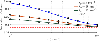
(a) $\Phi_{\rm u}$ is TCP.

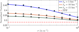
(b) $\Phi_{\rm u}$ is MCP.

Figure 1: Normalized variance of ${\Phi_{{\rm u}_{0}}}$ ($\lambda_{\rm b}=1\ \text{km}^{-2}$). The markers denote the values obtained by Monte Carlo simulation.

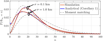
(a) $\Phi_{\rm u}$ is TCP

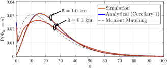
(b) $\Phi_{\rm u}$ is MCP

Figure 2: Load on ${\cal C}_{o}$: comparison of the proposed PMF and the actual PMF when $\Phi_{\rm u}$ is a TCP ($\lambda_{\rm b}=1\ {\rm km}^{-2}$, $\lambda_{\rm p}=5\ {\rm km}^{-2}$, $\bar{m}=5$), $R=1$, $N=128$.

III Moments of the Typical Cell Load

In this section, we will derive the $n$-th moment of ${\Phi_{{\rm u}_{0}}}$. We begin with the notion of the moment measure of $\Phi_{\rm u}$.

Definition 4 (Moment measure).

The $n$-th order moment measure of $\Phi_{\rm u}$ is defined as follows. Given $B_{1},\dots,B_{n}\in\mathfrak{B}_{\mathbb{R}^{2}}$,

$$\mu^{(n)}(B_{1}\times\dots B_{n}):=\mathbb{E}[\Phi_{\rm u}(B_{1})\dots\Phi_{\rm u}({B_{n}})]\\ =\mathbb{E}\bigg{[}\sum\limits_{\begin{subarray}{c}{\bf x}_{1},\dots,{\bf x}_{n}\\ \in\Phi_{\rm u}\end{subarray}}{\bf 1}({\bf x}_{1}\in B_{1})\dots\bf 1({\bf x}_{n}\in B_{n})\bigg{]}.$$ (4)

Plugging in $B_{i}=B,\forall\ i=1,\dots,n$ where $B\in\mathfrak{B}_{\mathbb{R}^{2}}$, we get $\mathbb{E}[(\Phi_{\rm u}(B))^{n}]=\mu^{(n)}(B^{n})$. However, we cannot simply replace $B$ with ${\cal C}_{o}$ in order to obtain $\mathbb{E}[({\Phi_{{\rm u}_{0}}})^{n}]$ since ${\cal C}_{o}$ is a random closed set. Using the moment measures, the expected summation over the points of the product PP $\Phi_{\rm u}^{n}\subset\mathbb{R}^{2n}$ can be expressed as an $n$-fold integral over $\mathbb{R}^{2}$. More formally, for a measurable function $g:\mathbb{R}^{2n}\mapsto\mathbb{R}^{+}$,

$$\mathbb{E}\bigg{[}\sum_{\begin{subarray}{c}{\bf x}_{1},\dots,{\bf x}_{n}\\ \in\Phi\end{subarray}}g({\bf x}_{1},\dots,{\bf x}_{n})\bigg{]}\\ =\int_{\mathbb{R}^{2}}\dots\int_{\mathbb{R}^{2}}g({\bf x}_{1},\dots,{\bf x}_{n})\mu^{(n)}({\rm d}{\bf x}_{1},\dots,{\bf x}_{n}).$$ (5)

Theorem 1.

The $n^{th}$ moment of ${\Phi_{{\rm u}_{0}}}$ for any general distribution of $\Phi_{\rm u}$ independent of $\Phi_{\rm b}$ can be written as: ${\mathbb{E}}[({{\Phi_{{\rm u}_{0}}}})^{n}]=\mathbb{E}[\mu^{(n)}({\cal C}_{o}^{n})]=$

$$\int\limits_{\mathbb{R}^{2}}\dots\int\limits_{\mathbb{R}^{2}}\exp\bigg{(}-\lambda_{\rm b}v_{2}\bigg{(}\bigcup\limits_{i=1}^{n}b({\bf x}_{i},\|{\bf x}_{i}\|)\bigg{)}\bigg{)}\mu^{(n)}({\rm d}{\bf x}_{1},\dots,{\rm d}{\bf x}_{n}).$$ (6)

Proof:

Following Definition 4, we can write

$${\mathbb{E}}[({{\Phi_{{\rm u}_{0}}}})^{n}]=\mathbb{E}[\mu^{(n)}({\cal C}_{o}^{n})]$$

$$={\mathbb{E}}\bigg{[}\sum\limits_{\{{\bf x}_{i}\}\in\Phi_{\rm u}}\prod\limits_{i=1}^{n}{\bf 1}({{\bf x}_{i}}\in{\cal C}_{o})\bigg{]}$$

$$\stackrel{{\scriptstyle(a)}}{{=}}{\mathbb{E}}\bigg{[}\sum\limits_{\{{\bf x}_{i}\}\in\Phi_{\rm u}}\mathbb{E}_{o}^{!}\bigg{(}\bigcap\limits_{{\bf y}\in\Phi_{\rm b}}\prod\limits_{i=1}^{n}{\bf 1}(\|{\bf x}_{i}\|<\|{\bf x}_{i}-{\bf y}\|)\bigg{)}\bigg{]}$$

$$=\mathbb{E}\bigg{[}\sum\limits_{\{{\bf x}_{i}\}\in\Phi_{\rm u}}{\mathbb{P}}\bigg{(}\Phi_{\rm b}\bigg{(}\bigcup\limits_{i=1}^{n}b({\bf x}_{i},\|{\bf x}_{i}\|\bigg{)}=0\bigg{)}\bigg{]}$$

$${=}{\mathbb{E}}\bigg{[}\sum\limits_{\{{\bf x}_{i}\}\in\Phi_{\rm u}}\exp\bigg{(}-\lambda_{\rm b}v_{2}\bigg{(}\bigcup\limits_{i=1}^{n}b({\bf x}_{i},\|{\bf x}_{i}\|)\bigg{)}\bigg{)}\bigg{]},$$

where $\mathbb{E}_{o}^{!}$ in $(a)$ is the expectation with respect to the reduced Palm distribution of $\Phi_{\rm b}$ which is same as its original distribution, by Slivnyak’s theorem [6, Theorem 8.3]. The last step is given by the void probability of PPP [6, Section 2.5]. The final expression is obtained by using (5). ∎

For stationary PPs, it is possible to simplify (6) for $n=1,2$. When $n=1$, $\mathbb{E}[{\Phi_{{\rm u}_{0}}}]=\lambda_{\rm u}\mathbb{E}[v_{2}({\cal C}_{o})]=\lambda_{\rm u}/\lambda_{\rm b}$, the stationarity of $\Phi_{\rm u}$ and $\Phi_{\rm b}$ imply $\mu^{(1)}(B)=\lambda_{\rm u}v_{2}(B)$ and $\mathbb{E}[v_{2}({\cal C}_{o})]=\lambda_{\rm b}^{-1}$, which is the mean area of ${\cal C}_{o}$ [6, Theorem 8.3]. If $\Phi_{\rm u}$ is a stationary and isotropic PP (which is indeed the case if $\Phi_{\rm u}$ is either TCP or MCP), we can write

$$\mathbb{E}[\Phi_{\rm u}^{2}(B)]=\mu^{(2)}(B^{2})=\lambda_{\rm u}v_{2}(B)\\ +\lambda_{\rm u}\int_{\mathbb{R}^{2}}\int_{\mathbb{R}^{2}}{\bf 1}({\bf x}_{1}\in B){\bf 1}({\bf x}_{2}\in B)\varrho^{(2)}(\|{\bf x}_{1}-{\bf x}_{2}\|)\>{\rm d}{\bf x}_{1}\>{\rm d}{\bf x}_{2},$$

where $\varrho^{(2)}(u)$ is called the second order moment density of $\Phi_{\rm u}$ [6, Section 6.4]. Then $\mathbb{E}[({\Phi_{{\rm u}_{0}}})^{2}]=\mathbb{E}[\mu^{(2)}({\cal C}_{o}^{2})]=$

$$\lambda_{\rm u}\mathbb{E}[v_{2}({\cal C}_{o})]+\lambda_{\rm u}\int_{\mathbb{R}^{2}}\int_{\mathbb{R}^{2}}\exp\big{(}-\lambda_{\rm b}\times v_{2}(b({\bf x}_{1},\|{\bf x}_{1}\|)$$

$$\cup b({\bf x}_{2},\|{\bf x}_{2}\|))\big{)}\varrho^{(2)}(\|{\bf x}_{1}-{\bf x}_{2}\|)\>{\rm d}{\bf x}_{1}{\rm d}{\bf x}_{2}\\ =\frac{\lambda_{\rm u}}{\lambda_{\rm b}}+\lambda_{\rm u}\int_{\mathbb{R}^{2}}\int_{\mathbb{R}^{2}}{\cal A}_{\rm u}(\|{\bf x}_{1}\|,\|{\bf x}_{2}\|,\|{\bf x}_{1}-{\bf x}_{2}\|)\\ \times\varrho^{(2)}(\|{\bf x}_{1}-{\bf x}_{2}\|)\>{\rm d}{\bf x}_{1}\>{\rm d}{\bf x}_{2}.$$

Now the second order moment density of PCP is given by $\varrho^{(2)}(r)=\lambda_{\rm u}^{2}(1+\lambda_{\rm p}^{-1}g(r))$ where $g(r)=\int_{\mathbb{R}}f_{\rm d}(r|0)f_{\rm d}(z+r|0)\>{\rm d}z$. This general expression of $\varrho^{(2)}(r)$ can be further simplified when ${\Phi_{{\rm u}_{0}}}$ is a TCP or a MCP: $\varrho^{(2)}(r)=$

$$\begin{cases}\lambda_{\rm p}^{2}\bar{m}^{2}+\frac{\lambda_{\rm p}\bar{m}^{2}}{4\pi\sigma^{2}}e^{-\frac{r^{2}}{4\sigma^{2}}},&\text{when $\Phi_{\rm u}$ is TCP}\\ \lambda_{\rm p}^{2}\bar{m}^{2}+{\bf 1}(r\leq 2{\tt R})\frac{\lambda_{\rm p}\bar{m}^{2}A_{\rm i}({\tt R},{\tt R},r)}{\pi^{2}{\tt R}^{4}},&\text{when $\Phi_{\rm u}$ is MCP}\end{cases},$$ (7)

where $A_{\rm i}({\tt R}_{1},{\tt R}_{2},r)=$ ${\tt R}_{1}^{2}\arctan\left(\frac{r^{2}+{\tt R}_{1}^{2}-{\tt R}_{2}^{2}}{t}\right)+{\tt R}_{2}^{2}\arctan\left(\frac{r^{2}-{\tt R}_{1}^{2}+{\tt R}_{2}^{2}}{t}\right)-\frac{t}{2},$ with $t=\big{(}({\tt R_{1}}+{\tt R}_{2}+r)({\tt R_{1}}+{\tt R}_{2}-r)({\tt R_{1}}-{\tt R}_{2}+r)(-{\tt R_{1}}$ $+{\tt R}_{2}+r)\big{)}^{\frac{1}{2}}$ and $0\leq r\leq{\tt R}_{1}+{\tt R}_{2}$. Interested readers are advised to refer to [6, Section 6.5] for the derivation of these results. We now present the mean and variance of ${\Phi_{{\rm u}_{0}}}$ in the following lemma.

Lemma 1.

When $\Phi_{\rm u}$ is a PCP, the first two moments of ${\Phi_{{\rm u}_{0}}}$ are given by: ${\mathbb{E}}[{\Phi_{{\rm u}_{0}}}]=\frac{\bar{m}\lambda_{\rm p}}{\lambda_{\rm b}},$ and ${\mathbb{E}}[({\Phi_{{\rm u}_{0}}})^{2}]=$

$$\frac{\lambda_{\rm u}}{\lambda_{\rm b}}+\int\limits_{0}^{2\pi}\int\limits_{0}^{\infty}\int\limits_{0}^{\infty}\exp(-\lambda_{\rm b}{A}_{\rm u}(x_{1},x_{2},d(x_{1},x_{2},\theta))\\ \times\varrho^{(2)}(d(x_{1},x_{2},\theta))x_{1}x_{2}\>{\rm d}x_{1}\>{\rm d}x_{2}{\rm d}\theta,$$

where $d(x_{1},x_{2},\theta):=(x_{1}^{2}+x_{2}^{2}-2x_{1}x_{2}\cos\theta)^{\frac{1}{2}}$.

${\rm Var}[{\Phi_{{\rm u}_{0}}}]=$

$$\begin{cases}\frac{\bar{m}^{2}\lambda_{\rm p}^{2}}{\lambda_{\rm b}^{2}}\left(0.28+\frac{2}{\lambda_{\rm p}\sigma^{2}}\int\limits_{0}^{\pi}\int\limits_{0}^{\infty}\int\limits_{0}^{x_{1}}\exp\left(-A_{\rm u}(x_{1},x_{2},d(x_{1},x_{2},\theta))-\frac{d(x_{1},x_{2},\theta)^{2}}{4\lambda_{\rm b}\sigma^{2}}\right)\>x_{1}\>x_{2}\>{\rm d}x_{2}\>{\rm d}x_{1}{\rm d}\theta\right),\\ \qquad\qquad\text{when $\Phi_{\rm u}$ is TCP,}\\ \frac{\bar{m}^{2}\lambda_{\rm p}^{2}}{\lambda_{\rm b}^{2}}\bigg{(}0.28+\frac{4}{\lambda_{\rm p}{\tt R}^{2}}\int\limits_{0}^{\infty}\int\limits_{0}^{\pi}\int\limits_{0}^{2{\tt R}}\exp\left(-\lambda_{\rm b}A_{\rm u}(x,(x^{2}+r^{2}+2xr\cos\theta),r)\right)A_{\rm i}({\tt R},{\tt R},r)\>x\>r\>{\rm d}r\>{\rm d}\theta\>{\rm d}x\bigg{)},\\ \qquad\qquad\text{ when $\Phi_{\rm u}$ is MCP.}\end{cases}$$ (8)

From Lemma 1, we can obtain the variance of ${\Phi_{{\rm u}_{0}}}$ which is given by (8) at the top of the next page. We skip the algebraic manipulation due to the lack of space. Note that the first term in (8) denotes the variance of ${\Phi_{{\rm u}_{0}}}$ if $\Phi_{\rm u}$ is a PPP. Also, $\mathbb{E}[{\Phi_{{\rm u}_{0}}}]$ is independent of the cluster size (which is $\sigma$ for TCP and $\tt R$ for MCP) and hence is the same as the mean cell load under the assumption that $\Phi_{\rm u}$ is a PPP of intensity $\bar{m}\lambda_{\rm p}$. However, the variance of ${\Phi_{{\rm u}_{0}}}$ is higher if $\Phi_{\rm u}$ is a PCP. The accuracy of (8) is verified in Fig. 1, where we see that the normalized variance ${\rm Var}[{\Phi_{{\rm u}_{0}}}]/\mathbb{E}[{\Phi_{{\rm u}_{0}}}]^{2}$ for TCP and MCP matches with the Monte Carlo simulations.

Remark 1.

Although Theorem 1 gives the exact expressions of the moments of ${\Phi_{{\rm u}_{0}}}$, we cannot go beyond the first two moments since the computation of (6) will be limited by the unavailability of the reduced moment measures of PCP for $n\geq 2$ in closed form. This motivates us to formulate a useful approximation to characterize the distribution of ${\Phi_{{\rm u}_{0}}}$, which will be presented in the next section.

With the expressions of the mean and variance of ${\Phi_{{\rm u}_{0}}}$, we now attempt to formulate the PMF of ${\Phi_{{\rm u}_{0}}}$ using moment matching. To this end, we assume that ${\Phi_{{\rm u}_{0}}}$ follows a negative binomial ($NB$) distribution, i.e., ${\Phi_{{\rm u}_{0}}}\sim NB(r,t)\Rightarrow\mathbb{P}({\Phi_{{\rm u}_{0}}}=n)={{r+n-1}\choose{n}}(1-t)^{r}t^{n}$ (for some $r\in{\mathbb{Z}}^{+},t\in(0,1]$). The intuition behind choosing $NB(r,t)$ is that given any closed subset $B\subset\mathbb{R}^{2}$, $\Phi_{\rm u}(B)$ follows a super-Poissonian distribution (i.e. the variance is greater than the mean), and $NB$ is a standard choice for approximating such random variables. By moment matching, we obtain $\hat{t}=1-\mathbb{E}[{\Phi_{{\rm u}_{0}}}]/{\rm Var}({\Phi_{{\rm u}_{0}}})$ and $\hat{r}=\lfloor(1-t)\mathbb{E}[{\Phi_{{\rm u}_{0}}}]/t\rfloor$. In Fig. 2, we plot the resulting PMF obtained by moment matching. We observe that for small cluster size (i.e. small $\sigma$ and $\tt R$ for TCP and MCP, respectively), the $NB$ PMF deviates significantly from the empirical PMF of ${\Phi_{{\rm u}_{0}}}$ obtained from simulation. In particular, the $NB$ distribution significantly underestimates the void probability $\mathbb{P}({\Phi_{{\rm u}_{0}}}=0)$. Hence the first two moments are not enough to characterize the distribution of ${\Phi_{{\rm u}_{0}}}$. Since obtaining the exact expressions of higher order moments is not possible using this route, we provide an alternate formulation for the PMF of ${\Phi_{{\rm u}_{0}}}$ in the next section.

IV Derivation of the Load PMF

This is the second contribution of the letter, where we start from an approximation of the typical PV cell which eventually leads us to a reasonably accurate characterization of the load PMF. In order to enable the analysis, we approximate the typical cell as a circle with the same area. We formally state this approximation as follows.

Assumption 1.

We assume that $\Phi_{\rm u}({\cal C}_{o})\approx\Phi_{\rm u}(b(o,R_{\rm c}))$, where $\pi R_{\rm c}^{2}=v_{2}({\cal C}_{o})$.

While this approximation is inspired by the fact that the large cells in a PV tessellation are circular  [7, Theorem 4], we will demonstrate that this approximation provides reasonably accurate characterization of the PMF of ${\Phi_{{\rm u}_{0}}}$ in the non-asymptotic regime as well. We first characterize the PGF of ${\Phi_{{\rm u}_{0}}}$ in the following theorem.

Theorem 2.

The PGF of ${\Phi_{{\rm u}_{0}}}$ is given as: $G_{{\Phi_{{\rm u}_{0}}}}(\theta)=$

$${\mathbb{E}}\big{[}\theta^{{\Phi_{{\rm u}_{0}}}}\big{]}=\int\limits_{0}^{\infty}\exp\bigg{(}-2\pi\lambda_{\rm p}\int\limits_{0}^{\infty}\bigg{(}1-\exp\bigg{(}-\bar{m}\\ \times\int\limits_{0}^{r}(1-\theta)f_{\rm d}(u|v){\rm d}{u}\bigg{)}\bigg{)}v{\rm d}v\bigg{)}f_{R_{\rm c}}(r){\rm d}{r},$$ (9)

where $f_{R_{\rm c}}(r)={\frac{2\times 3.5^{3.5}}{\Gamma(3.5)}r^{6}\exp\left(-{3.5r^{2}}\right)}$.

Proof:

Following [8], the random variable $\lambda_{\rm b}v_{2}({\cal C}_{o})$ follows a Gamma distribution with PDF: $f(x;\alpha,\beta)=\frac{\beta^{-\alpha}}{\Gamma(\alpha)}x^{\alpha-1}e^{-\frac{x}{\beta}},\ x>0,$ where $\alpha=3.5$ and $\beta=3.5^{-1}$. Since $\pi R_{\rm c}^{2}=v_{2}({\cal C}_{o})$, $\sqrt{\pi\lambda_{\rm b}}R_{\rm c}$ follows a Nakagami distribution with PDF $f_{R_{\rm c}}(x;m,\Omega)={\frac{2m^{m}}{\Gamma(m)\Omega^{m}}}x^{2m-1}\exp\left(-{\frac{m}{\Omega}}x^{2}\right),\ x>0,$ where $m=3.5$ and $\Omega=1$. We now focus on the conditional PGF of $\Phi_{\rm u}(b(o,R_{\rm c}))$ given $R_{\rm c}$: $G_{\Phi_{\rm u}(b(o,R_{\rm c}))}(\theta)=\mathbb{E}\left[\theta^{\Phi_{\rm u}(b(o,R_{\rm c}))}\right]=\mathbb{E}\left[\theta^{\sum\limits_{{\bf x}\in\Phi_{u}}{\bf 1}(\|{\bf x}\|<R_{\rm c})}\right]=\mathbb{E}\left[\prod\limits_{{\bf x}\in\Phi_{u}}\theta^{{\bf 1}(\|{\bf x}\|<R_{\rm c})}\right].$ The final step follows from the PGFL of PCP [3, Lemma 4] and deconditioning over $R_{\rm c}$. ∎

We now evaluate $G_{\Phi_{\rm u}({\cal C}_{o})}(\theta)$ when $\Phi_{\rm u}$ is a TCP (MCP).

Corollary 1.

When $\Phi_{\rm u}$ is a TCP, $G_{\Phi_{\rm u}({\cal C}_{o})}(\theta)=$

$$\int\limits_{0}^{\infty}\exp\bigg{(}-2\pi\lambda_{\rm p}\int\limits_{0}^{\infty}\big{(}1-\exp\big{(}-\bar{m}(1-\theta)\\ \times\big{(}1-Q_{1}({v}{\sigma}^{-1},{r}{\sigma}^{-1})\big{)}\big{)}\big{)}v{\rm d}v\bigg{)}f_{R_{\rm c}}(r){\rm d}r,$$ (10)

where $Q_{1}(\alpha,\beta)=\int_{\beta}^{\infty}ye^{-\frac{y^{2}+\alpha^{2}}{2}}I_{0}(\alpha y){\rm d}{y}$ is the Marcum Q-function. Here $I_{0}(\cdot)$ is the modified Bessel function of order zero. When $\Phi_{\rm u}$ is an MCP, $G_{\Phi_{\rm u}({\cal C}_{o})}(\theta)$ is given by:

$$\int\limits_{0}^{\infty}\exp\bigg{(}-2\pi\lambda_{\rm p}\int\limits_{0}^{\infty}\big{(}1-\exp\big{(}-\bar{m}(1-\theta)\\ \times\xi(r,v)\big{)}\big{)}v{\rm d}v\bigg{)}f_{R_{\rm c}}(r){\rm d}{r},$$ (11)

where

$$\xi(r,v)=\frac{1}{{\tt R}^{2}}\bigg{(}\big{[}\min(r,\max({\tt R}-v,0))\big{]}^{2}\\ +\frac{2}{\pi}\int\limits_{\min(r,|{\tt R}-v|)}^{\min(r,{\tt R}+v)}u\arccos\bigg{(}\frac{u^{2}+v^{2}-{\tt R}^{2}}{2uv}\bigg{)}{\rm d}u\bigg{)}.$$

Finally the PMF of ${\Phi_{{\rm u}_{0}}}$, denoted as $\{p_{n},n\geq 0\}$, can be obtained by performing the inverse $z$-transform of the PGF which is given by:

$$p_{n}=\frac{R^{n}}{2}\int\limits_{-\pi}^{\pi}G_{{\Phi_{{\rm u}_{0}}}}(Re^{j\theta})e^{jn\theta}{\rm d}\theta,$$ (12)

where $R$ is chosen such that $G_{{\Phi_{{\rm u}_{0}}}}(Re^{j\theta})$ is finite for all $-\pi<\theta<\pi$. For numerical computation, (12) can be approximated as a summation at $N$ distinct points:

$$\hat{p}_{n}=\frac{R^{n}}{N}\sum\limits_{m=0}^{N-1}G_{{\Phi_{{\rm u}_{0}}}}(Re^{j2\pi m/N})e^{j2\pi nm/N}.$$ (13)

Note that this step is nothing but the inverse discrete Fourier transform (DFT) of $\{G_{{\Phi_{{\rm u}_{0}}}}(Re^{j2\pi m/N}),m=0,1,\dots,N-1\}$, scaled by $R^{n}$ [9]. The Matlab scripts for the evaluation of (13) are available in [10]. In Fig. 2, we observe that $\{\hat{p}_{n}\}$ closely approximates the true PMF $\mathbb{P}({\Phi_{{\rm u}_{0}}}=n)$, which is empirically computed from the Monte Carlo simulations of the network.

V Application to Rate Analysis

In this section, we will apply the PMF of ${\Phi_{{\rm u}_{0}}}$ to characterize the downlink rate in the cellular network under the system model defined in Section II. In particular, we evaluate the complementary cumulative density function (CCDF) of rate for a representative user, which is selected uniformly at random from ${\Phi_{{\rm u}_{0}}}$ conditioned on the fact that the typical cell has at least one user, i.e., ${\Phi_{{\rm u}_{0}}}>0$. Assuming that this user is located at ${\bf u}$, the signal-to-interference-ratio ($\mathtt{SIR}$) is defined as:

$$\mathtt{SIR}=\frac{h_{{o}}\|{\bf u}\|^{-\alpha}}{\sum\limits_{{\bf x}\in\Phi\setminus\{{o}\}}h_{{\bf x}}\|{\bf x}-{\bf u}\|^{-\alpha}}.$$ (14)

Here $h_{{\bf x}}$ denotes fading on the link between the representative user and the BS at ${\bf x}\in\Phi_{\rm b}$, and $\alpha>2$ is the pathloss exponent. We assume Rayleigh fading, i.e., $\{h_{\bf x}\}$ is a sequence of i.i.d. random variables with $h_{\bf x}\sim\exp(1)$. Assuming interference-limited network and the system bandwidth (BW) ($W$) is equally partitioned between the users associated with a BS, the rate of the representative user conditioned on $\Phi_{\rm u}({\cal C}_{o})>0$ is defined as: ${\tt Rate}=\min\big{(}\frac{W}{{\Phi_{{\rm u}_{0}}}}\log(1+\mathtt{SIR}),\frac{R_{\rm b}}{{\Phi_{{\rm u}_{0}}}}\big{)},$ where $R_{\rm b}$ is the backhaul constraint on the BS imposed by the fiber connecting the BS to the network core which can support a maximum rate of $R_{\rm b}\ \text{bps}$. Hence the rate of each user cannot exceed $R_{\rm b}/{\Phi_{{\rm u}_{0}}}$. We define the rate coverage probability as the CCDF of $\tt Rate$: $\mathtt{P_{r}}(\rho)=\mathbb{P}({\tt Rate}>\rho|{\Phi_{{\rm u}_{0}}}>0)$, where $\rho$ is the target rate threshold. We now provide the expression for the rate coverage in the following theorem.

Theorem 3.

The rate coverage probability for the representative user is expressed as:

$$\mathtt{P_{r}}(\rho)\approx\sum\limits_{n=1}^{\lfloor\frac{R_{\rm b}}{\rho}\rfloor}\mathtt{P_{c}}\bigg{(}2^{\frac{n\rho}{W}-1}\bigg{)}\frac{\hat{p}_{n}}{1-\hat{p}_{0}},$$ (15)

where $\hat{p}_{n}$ is obtained from (13) and $\mathtt{P_{c}}(\tau)=\mathbb{P}(\mathtt{SIR}>\tau)$ is the CCDF of $\mathtt{SIR}$ that can be expressed as:

$$\mathtt{P_{c}}(\tau)=\delta^{2}\tau^{-\frac{2}{\alpha}}\int\limits_{0}^{\tau^{\frac{2}{\alpha}}}\frac{\beta(t)^{-2}}{1+t^{\frac{\alpha}{2}}}{\rm d}t,$$ (16)

where $\beta(t)=t\int\limits_{t^{-1}}^{\infty}\frac{1}{1+u^{\frac{2}{\alpha}}}{\rm d}u$, with $\delta=\frac{9}{7}$.

Proof:

Given the backhaul constraint, the maximum users that can be supported with a rate $\rho$ is given by $\lfloor R_{\rm b}/\rho\rfloor$. First we note that $\tt Rate$ is a function of $\mathtt{SIR}$ and ${\Phi_{{\rm u}_{0}}}$, which are in general correlated. However, the joint distribution of $\mathtt{SIR}$ and ${\Phi_{{\rm u}_{0}}}$ is intractable. For tractability, we assume that these two random variables are independent. This is a well-accepted assumption in the literature that preserves the accuracy of the analysis [2, Section 3]. Under this assumption, the rate coverage can be expressed as: $\mathtt{P_{r}}(\rho)=\mathbb{P}\big{(}\frac{W}{\Phi_{\rm u}({\cal C}_{o})}\log(1+\mathtt{SIR})>\rho|\Phi_{\rm u}({\cal C}_{o})>0\big{)}=$ $\mathbb{P}\bigg{(}\mathtt{SIR}>2^{\frac{\Phi_{\rm u}({\cal C}_{o})\rho}{W}}-1\big{|}\Phi_{\rm u}({\cal C}_{o})>0\bigg{)}=$

$$=\sum\limits_{n=1}^{\lfloor\frac{R_{\rm b}}{\rho}\rfloor}\overbrace{\mathtt{P_{c}}(2^{n\rho/W}-1)}^{\text{$\mathtt{SIR}$ distribution}}\times\underbrace{\mathbb{P}({\cal C}_{o}(\Phi_{\rm u})=n|{\cal C}_{o}(\Phi_{\rm u})>0)}_{\text{load distribution}}.$$

The load distribution can be simplified as: $\frac{\mathbb{P}({\cal C}_{o}(\Phi_{\rm u})=n,{\cal C}_{o}(\Phi_{\rm u})>0)}{\mathbb{P}({\cal C}_{o}(\Phi_{\rm u})>0)}$. Hence we are left with the characterization of $\mathtt{P_{c}}$, or the CCDF of $\mathtt{SIR}$. Since $\Phi_{\rm u}$ and $\Phi_{\rm b}$ are independent and $\Phi_{\rm u}$ is a stationary distribution (i.e. the distribution of $\Phi_{\rm u}$ is invariant under translation of its points), the representative user is equivalent to a randomly selected point in ${\cal C}_{o}$. The $\mathtt{SIR}$ distribution of this point has been recently characterized in [11]. The expression of $\mathtt{P_{c}}(\tau)$ in (16) is obtained from [11, Theorem 2]. ∎

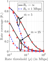
(a)

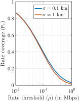
(b)

Figure 3: Rate coverage probability: 3(a) for different $\bar{m}$ (markers indicate the values obtained from Monte Carlo simulation) and 3(b) for different $\sigma$ with $R_{\rm b}\to\infty$ ($(\lambda_{\rm b},\lambda_{\rm p})=(1,5)\text{km}^{-2}$ and $W=1$ MHz).

We verify the accuracy of Theorem 3 in Fig. 3(a) which exhibits a close match between the analytical and empirical results. Because of the space constraint, we only present the results when $\Phi_{\rm u}$ is a TCP. We observe that $\mathtt{P_{r}}$ decreases as (i) $\bar{m}$ increases as more number of users share the resources and (ii) $R_{\rm b}$ decreases as it imposes an upper bound on the per user rate. In Fig. 3(b), we plot $\mathtt{P_{r}}$ for different $\sigma$ which is a measure of the cluster size. We further observe that $\mathtt{P_{r}}$ is almost invariant to $\sigma$. The reason is that the rate coverage is mostly dominated by the first moment of load (see [1, Corollary 1]) which is independent of the cluster size.

VI Conclusion

Due to the limitation of PPP in modeling spatial coupling between the nodes, there has been increasing interests in developing non-PPP models of cellular networks, such as the PCP-based models which capture coupling between the users (such as in hotspots) and between users and BSs [3]. While the $\mathtt{SINR}$ distribution for the PCP-based models is by now well-understood, the load distribution in these networks has not received much attention. In this letter, we made the first attempt towards this direction by characterizing the distribution of the typical cell load where the BSs are distributed as a homogeneous PPP and the users are distributed as an independent PCP. We also demonstrated the utility of this result by using it to characterize the user rate for a representative user in the typical cell.

References

[1]
S. Singh, H. S. Dhillon, and J. G. Andrews, “Offloading in heterogeneous
networks: Modeling, analysis, and design insights,” IEEE Trans. on
Wireless Commun., vol. 12, no. 5, pp. 2484–2497, May. 2013.
[2]
H. S. Dhillon and J. G. Andrews, “Downlink rate distribution in heterogeneous
cellular networks under generalized cell selection,” IEEE Wireless
Commun. Letters, vol. 3, no. 1, pp. 42–45, Feb. 2014.
[3]
C. Saha, M. Afshang, and H. S. Dhillon, “3GPP-inspired HetNet model
using Poisson cluster process: Sum-product functionals and downlink
coverage,” IEEE Trans. on Commun., vol. 66, no. 5, pp. 2219–2234,
May 2018.
[4]
V. V. Chetlur and H. S. Dhillon, “Coverage and rate analysis of downlink
cellular vehicle-to-everything (C-V2X) communication,” IEEE Trans.
on Wireless Commun., vol. 19, no. 3, pp. 1738–1753, Mar. 2020.
[5]
G. George, A. Lozano, and M. Haenggi, “Distribution of the number of users per
base station in cellular networks,” IEEE Wireless Commun. Letters,
vol. 8, no. 2, pp. 520–523, 2018.
[6]
M. Haenggi, Stochastic Geometry for Wireless Networks. Cambridge University Press, 2012.
[7]
P. D. Mankar, P. Parida, H. S. Dhillon, and M. Haenggi, “Distance from the
nucleus to a uniformly random point in the -cell and the typical cell of
the Poisson-Voronoi tessellation,” 2019, available online:
arXiv/abs/1907.03635.
[8]
J.-S. Ferenc and Z. Néda, “On the size distribution of Poisson Voronoi
cells,” Physica A: Statistical Mechanics and its Applications, vol.
385, no. 2, pp. 518–526, 2007.
[9]
J. Cavers, “On the fast fourier transform inversion of probability generating
functions,” IMA Journal of Applied Mathematics, vol. 22, no. 3, pp.
275–282, 1978.
[10]
C. Saha and H. S. Dhillon, “Matlab code for the computation of the PMF of
the number of points of a PCP in a typical cell of a stationary PPP,”
available at: https://github.com/stochastic-geometry/LoadDistributionPCP.
[11]
P. D. Mankar, P. Parida, H. S. Dhillon, and M. Haenggi, “Downlink analysis for
the typical cell in Poisson cellular networks,” IEEE Wireless
Commun. Letters, vol. 9, no. 3, pp. 336–339, Mar. 2020.