A semiclassical theory of the chemical potential for the Atomic Elements

Abstract

The chemical potiential for the ground states of the atomic elements have been calculated within the semiclassical approximation The present work closely follows Schwinger and Englert’s semiclassical treatment of atomic structure.

1 The Chemical Potential $\mu$ of the Atomic Elements

For an atomic element containing $N$ electrons with nuclear charge $Z$, the electronic chemical potentials $\mu$ for neutral atomic species (which are in their electronic ground states $\Psi$ with energy $E$) are defined as

$$\mu=\left(\frac{\partial E}{\partial N}\right)_{Z}\text{.}$$

Here $N$ and $Z$ will be regarded as continuous variables and $\mu$ can then be calculated by noting that

$$dE(Z,N)=\left(\frac{\partial E}{\partial Z}\right)_{N}dZ+\left(\frac{\partial E}{\partial N}\right)_{Z}dN,$$

together with the well-known relation

$$\left(\frac{\partial E}{\partial Z}\right)_{N}=\frac{\overline{V}_{ne}}{Z}.$$

In the equation above, $\overline{V}_{ne}$ is the average value of the nuclear-electronic potential energy (in atomic units) i.e.

$$\frac{\overline{V}_{ne}}{Z}=-\sum_{i=1}^{N}\int\frac{\left|\Psi_{0}\right|^{2}}{r_{i}}d\tau,$$

and $d\tau=d\mathbf{r}_{1}d\mathbf{r}_{2}d\mathbf{r}_{3}\ldots d\mathbf{r}_{N}.$  We have as a result

$$\mu=\frac{d\,E(Z,Z)}{d\,Z}-\frac{\overline{V}_{ne}}{Z},$$ (1)

where $dE/dZ$ is the directional derivative of the electronic energy surface $E(Z,N)$ along the curve $Z=N.$  In this work $E(Z,Z)$ is taken to be the electronic energy which has been computed within the semiclassical approximation by Schwinger and Englert.

1.1 Properties and estimates of the chemical potential for the elements

The physical interpretation or significance of the electronic chemical potential $\mu$ is seen as a measure of the propensity of an electron to leave an atom.  In this context as the atomic number increases $\mu$ gives the stability of an element relative to others in the periodic table.

An associated quantity $\eta$ defined by

$$\eta=\frac{1}{2}\left(\frac{\partial\mu}{\partial N}\right)_{Z}\text{,}$$

has been called the hardness [1] and has been interpreted as the resistance of an atom to the ingress of additional electrons. The higher the hardness the the lower the polarizability of the atom’s electron cloud and the greater the resistance of that atom to add an electron.  Various estimates for the chemical potential and the hardness have been made.  March [2] has given an estimate of $\mu$ by assuming that the energy can be written as a Taylor series in the variable $(N-Z)$ i.e.

$$E(Z,N)=E(Z,Z)+(N-Z)\left(\frac{\partial E}{\partial N}\right)|_{Z=N}+\frac{(N-Z)^{2}}{2}\left(\frac{\partial^{2}E}{\partial N^{2}}\right)|_{Z=N}+\cdots.$$

In that work he has shown that to third order (from a fifth order polynomial in  $N-Z$ ) that the chemical potential can be written as

$$\mu=\mu_{2}+\mu_{3},$$

with

$$\mu_{2} =-\tfrac{1}{2}(I_{1}+A),$$

$$\mu_{3} =\tfrac{1}{60}\left(3I_{4}-17I_{3}+43I_{2}-47I_{1}+18A\right),$$

and where $I_{n}$ is the n-th ionization potential of the atom and $A$ is it’s electron affinity.  Using the empirical relation $I_{n}\cong nI_{1}$ the chemical potential to third order $\mu_{3}=\frac{3}{10}A$ and we have two estimates

$$\mu=-\tfrac{1}{2}(I_{1}+A),$$

to lowest order and

$$\mu=-\tfrac{1}{2}I_{1}-\tfrac{1}{5}A,$$

which includes $\mu_{3}.$  It is interesting to note that Mulliken’s electronegativity function $\chi_{M}$ which is defined as

$$\chi_{M}\equiv\tfrac{1}{2}(I_{1}+A)>0,$$

and is interpreted as the ability of an atom to attract electrons is approximately related to $-\mu$.  Piris and March [3] using natural orbital functional (NOF) theory have estimated $\mu$ and compared it to $-\,I_{1}$ for neutral atom (H-Kr) as seen in the Fig.(1) below.

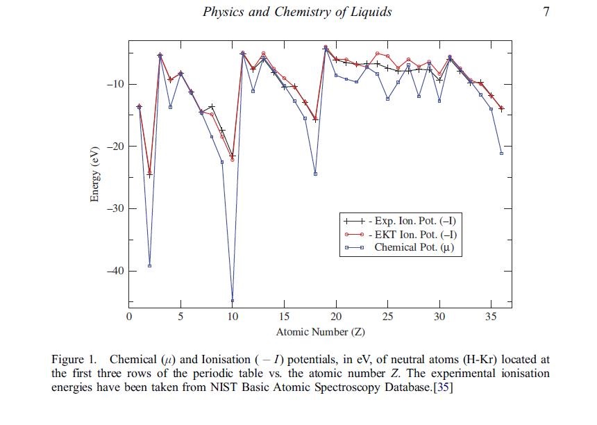
Figure 1: The Chemical Potential $\mu$ vs. Z.

Their chemical potential values parallel the oscillations in the experimental ionization potential but deviate widely in magnitude from $-\,I_{1}$ in case of the rare gases. If one wishes to interpret the electronic chemical potential as the atomic analogue of the macroscopic thermodynamic chemical potential, then $\mu$ as define above is an indication of the spontaneity of the escaping tendency of an electron from an atom.

1.2 A Semiclassical Approximation for the chemical potential $\mu$

Within the “semiclassical approximation,” Schwinger and Englert [4] (SE) have given an expression for $E(Z,Z)$.  In that work, the authors have shown that the total energy is made up of the semiclassial i.e. Thomas-Fermi (TF) energy [5] and a quantum oscillating part i.e.

$$E(Z,Z)=E_{TF}(Z,Z)+E_{\,osc}(Z).$$

Furthermore, the well-known value for $E_{TF}(Z,Z)$ is given by [6]

$$E_{TF}\,(Z,Z)=\tfrac{6}{7}\left(\tfrac{4}{3\pi}\right)^{2/3}\Phi^{\prime}(0)\,Z^{\,7/3},$$ (2)

with $\Phi^{\prime}(0)=-1.588071$ [7] being the initial slope of the TF function $\Phi(x)$ and where the TF potential $V_{TF}$ is

$$V_{TF}=-Z\,\Phi(x)/r,$$

and $x$ is the TF scaled distance $x=2^{7/3}r/(3\pi)^{2/3}$ The average value of the TF potential energy is [8]

$$\overline{V}_{TF}=-Z\,\int_{0}^{\infty}\frac{\rho(\mathbf{r})}{r}d\mathbf{r=}2\left(\tfrac{4}{3\pi}\right)^{2/3}\Phi^{\prime}(0)\,Z^{\,7/3}.$$ (3)

We shall see below that the average value of the nuclear-electronic potential $\overline{V}_{ne}$ like the total energy, can also be written as a sum of a TF term and a quantum oscillating contribution i.e.

$$\overline{V}_{ne}=\overline{V}_{TF}+\overline{V}_{osc}.$$

As a result of (2) and (3) the TF part to the chemical potential is seen to vanishes,

$$\mu_{TF}=0,$$

there being no contribution of order $Z^{\,4/3}$and we have as a result

$$\mu=\frac{dE(Z,Z)_{osc}}{dZ}-\frac{\overline{V}_{ne,\,osc}}{Z}.$$

The purpose of this work is to give the corresponding semiclassical expression for $\overline{V}_{ne,osc}$ resulting in a semiclassical value for the chemical potential for neutral atomic species.  As will be seen below the computation of that quantity unfortunately requires a rather elaborate analysis. This investigation does not contain the effects due to the antisymmetry [9] of the system’s wave functions or the effects of the tightly bound electrons first taken into account by Scott [10] nor the quantum correction to the wave function due to the kinetic energy [11].  Inclusion of these effects is problematic and beyond the scope of this work.

We begin the analysis of $\overline{V}_{ne}$ by recognizing that since the terms within $\overline{V}_{ne\text{ }}$are single-particle operators, integration over the $N-1$ coordinates of the $N$ particle wave function reduces $\overline{V}_{ne}$ to

$$-\frac{\overline{V}_{ne}}{Z}=\int\frac{\varrho(\mathbf{r})}{r}d\mathbf{r},$$

where $\varrho$ is the single-particle electron density function defined as

$$\varrho(\mathbf{r})=N\int\ldots\int\left|\Psi\right|^{2}d\mathbf{r}_{2}d\mathbf{r}_{3}\ldots d\mathbf{r}_{N}.$$

This function could for example be taken to be the Thomas-Fermi electron density.  Instead, within the semi-classical (WKB) [12], and the Hartree-Fock orbital approximations we take the density to be

$$\varrho(\mathbf{r})=2\sum_{l=0}^{\infty}\sum_{n_{r}=0}^{\infty}(2l+1)\eta(-E_{l,n_{r}}-\zeta)\,\,|u_{l,n_{r}}(r)/\sqrt{4\pi}r|^{2}.$$ (4)

The single particle energies $E_{l,n_{r}}$ associated with the potential $V(r)$ are labeled with the radial quantum number $n_{r}$ and the angular quantum number $l$ respectively and the quantities $u\,_{l,\,n_{r}}(r)/\sqrt{4\pi}r$ are the WKB single-particle semiclassical wave functions where $-\,\zeta$ is the single-particle energy of the highest occupied orbital ($\zeta\geq 0$), and $\eta$ is the Heaviside function as shown in Fig. (2) below.

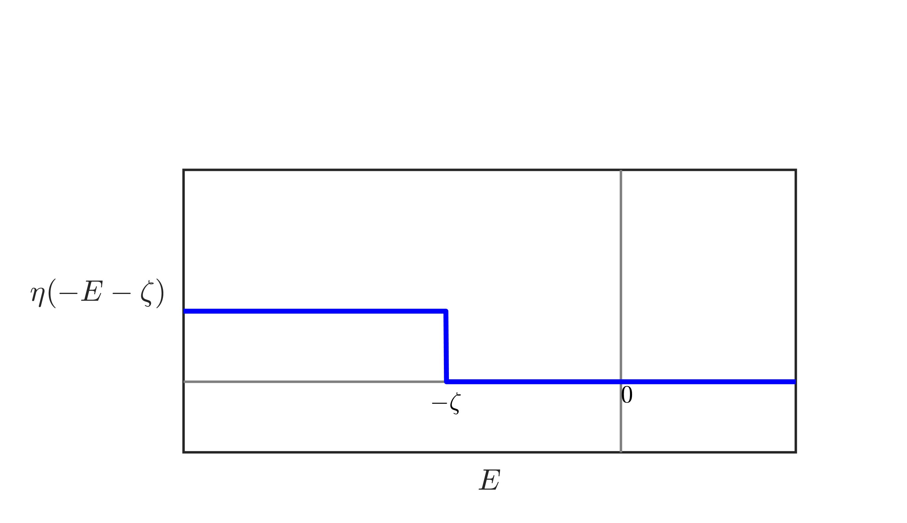
Figure 2: The Heaviside function vs. Energy.

The latter function having been introduced in order to provide cutoffs in the sums in (4) over the positive integer quantum numbers $l,$ $n_{r}$ thereby removing energies larger than $-\,\zeta$.  The factor of 2 in Eq.(4) has been included in the sum to account for the spin states.  Using (4) we have

$$\overline{V}_{ne}=2\sum_{l=0}^{\infty}\sum_{n_{r}=0}^{\infty}(2l+1)\,\eta(-E_{l,\,n_{r}}-\varsigma)\overline{V}_{l,n_{r}},$$ (5)

with

$$\overline{V}_{l\,,\,n_{r}}=-Z\int_{r_{l}}^{r_{u}}\frac{\left|u_{l\,,\,n_{r}}(r)\right|^{2}}{r}dr,$$

and $r_{l}$ and $r_{u}$ are the WKB lower and upper classical turning points which define the classically allowed region.  The WKB functions $u_{l,n_{r}}(r)$ being given by

$$u_{l,n_{r}}(r)=\frac{A_{l,n_{r}}}{\sqrt{2}\,\left[2\{E_{l,n_{r}}-V(r)-{\small(}l{\small+}1/2{\small)}^{2}{\small/}2r^{2}\}\right]^{1/4}},$$ (6)

where $A_{l,n_{r}}$ are normalization constants and $V(r)$ is a central but not necessarily the Coulombic potential (The $r$ dependencies of the “phase factors” [13] of these functions are being ignored here).  The potential $V(r)$ represents the interaction of an electron with the nuclear charge as well as with the other electrons in the atom, an approximate example of which is the TF potential.

Within the WKB approximation one also has the relation

$$n_{r}+1/2\,{\small=}\frac{1}{\pi}\int_{r_{l}}^{r_{u}}\sqrt{2\{E_{l,n_{r}}-V(r)-{\small(}l{\small+}1/2{\small)}^{2}{\small/}2r^{2}\}}\,dr,$$ (7)

where $r_{l}$ and $r_{u}$ referred to above are the roots of the quantity within the square root of that expression.  Following Schwinger and Englert [14] we define the quantities $\lambda,\nu,\varepsilon_{\lambda,\nu},$and $\upsilon_{\lambda,\nu}$ as

$$\lambda =l+1/2,$$

$$\nu =n_{r}+1/2,$$

$$\varepsilon_{\lambda,\nu} =E_{l\,,\,n_{r}},$$

$$\upsilon_{\lambda,\nu} =\overline{V}_{l\,,\,n_{r}},$$

and regard them as continuous variables in the equations below. Then (7) becomes

$$\nu=\frac{1}{\pi}\int_{r_{l}}^{r_{u}}\sqrt{2\{\varepsilon_{\lambda,\nu}-V(r)-\lambda^{2}{\small/}2r^{2}\}}\,dr.$$ (8)

Rewriting (5), we note that the sums now extend over the negative as well as the positive values of $l$ and $n_{r}$.  The former values however, do not contribute to the sums and we get

$$\overline{V}_{ne}=4\int_{0}^{\infty}\lambda d\lambda\sum_{l=-\infty}^{\infty}\delta(l+1/2-\lambda)\int_{0}^{\infty}d\nu\sum_{n_{r}=-\infty}^{\infty}\delta(n_{r}+1/2-\nu){\large\upsilon}_{\lambda,\nu}\eta(-\varepsilon_{\lambda,\nu}-\varsigma),$$

where $\delta(z)$ is the Dirac delta function.  Using the Poisson identities

$$\sum_{l=-\infty}^{\infty}\delta(l+1/2-\lambda) =\sum_{k=-\infty}^{\infty}(-1)^{k}\exp(2\pi ik\lambda),$$

$$\sum_{n_{r}=-\infty}^{\infty}\delta(n_{r}+1/2-\nu)\, =\sum_{j=-\infty}^{\infty}(-1)^{j}\exp(2\pi ij\nu),$$

the expression for $\overline{V}_{ne}$ becomes

$$\overline{V}_{ne}=4\sum_{k=-\infty}^{\infty}\;\sum_{j=-\infty}^{\infty}(-1)^{k+j}\int_{0}^{\infty}\lambda\exp(2\pi ik\lambda)d\lambda\int_{0}^{\infty}\exp(2\pi ij\nu)\,{\large\upsilon}_{\lambda,\nu}\eta(-\varepsilon_{\lambda,\nu}-\varsigma)\,d\nu.$$ (9)

1.3 Interrelations Among The Variables $\lambda\,,\nu$  And $\varepsilon(\lambda\,,\nu)$

Before proceeding, it is useful to examine the relations among the quantities $\nu$, $\lambda$ and $\varepsilon(\lambda,\nu).$  For a given $V(r)$ and energy $\varepsilon,$ and for a range of values of $\nu$ which will be discussed below, the roots of the relation

$$2r^{2}[\varepsilon_{\lambda,\nu}-V(r)]-\lambda(r)^{2}=0,$$ (10)

i.e. $r_{l}$ and $r_{u},$ define the classical turning points for the system.  We note that it follows from Eq. (4) that when $\nu=0$, that these roots coalesce to the single value of $r_{\varepsilon}.$  This behavior can be seen graphically in Fig. (3) where  we have plotted the effective potential $V^{\prime}=V(r)+\lambda^{2}/2r^{2}$ versus $r$.

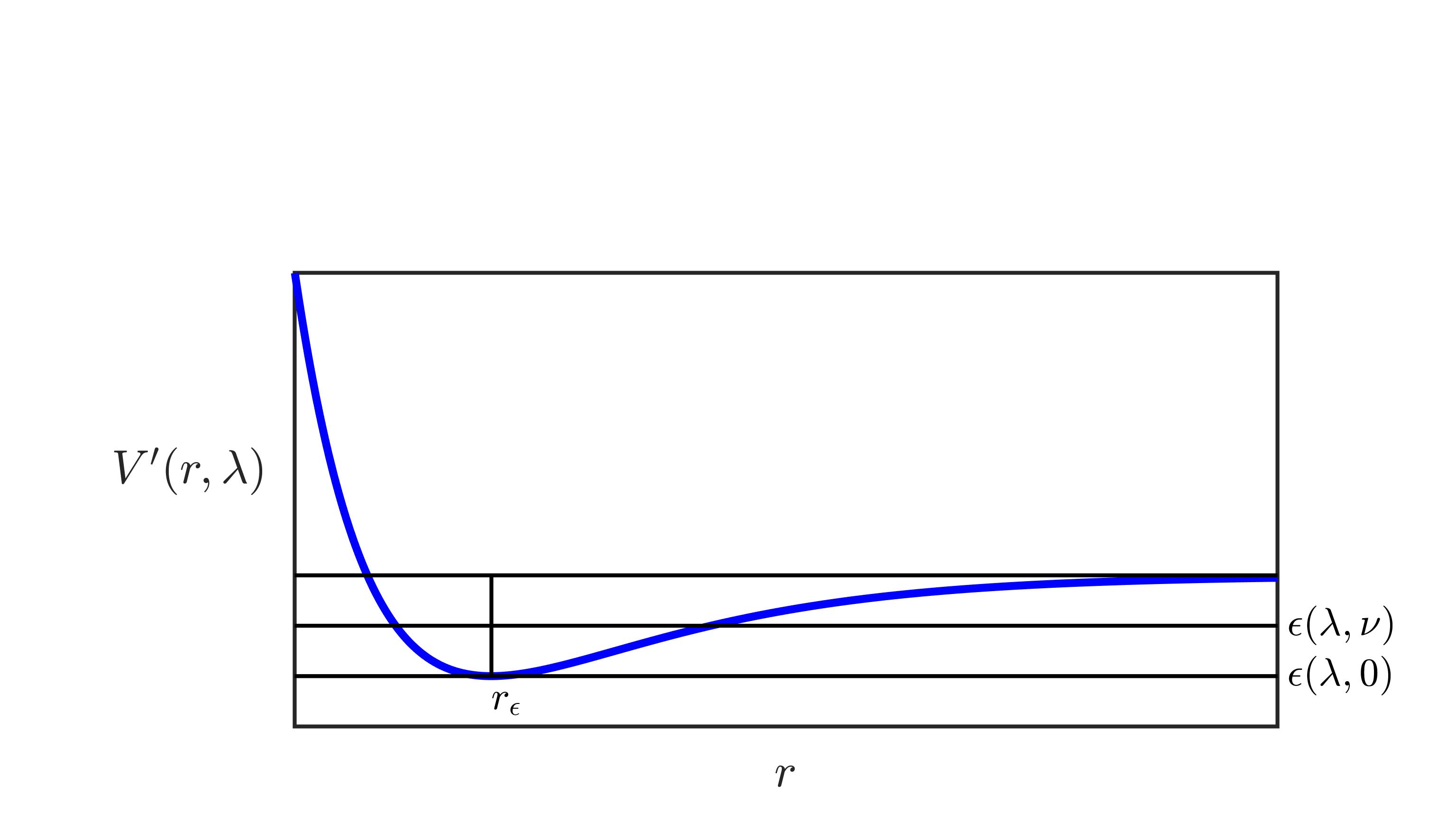
Figure 3: The Effective potential vs. r

For a given energy $\varepsilon(\lambda_{\varepsilon},0)$ the curve $V^{\,\prime}(r)$ is seen to have a single turning point denoted by $r_{\varepsilon}.$  However, the curve $V^{\,\prime}(r)$ for any $\varepsilon(\lambda,\nu)>\varepsilon(\lambda_{\varepsilon},0)$ has two turning points $r_{l},$ $r_{u}$ which are less than and greater than $r_{\varepsilon}$.  Recalling that these turning points are the roots of Eq. (8) we will see in what follows that $r_{\varepsilon}$ is the distance at which $\lambda$ has it maximum value i.e. $\lambda_{\varepsilon}.$  This value is given by

$$\lambda_{\varepsilon}(r_{\varepsilon})=\sqrt{2r_{\varepsilon}^{2}\left\{\varepsilon(\lambda_{\varepsilon},0)-V(r_{\varepsilon})\right\}}.$$

Furthermore, in the case where the single-particle energy has its absolute highest value referred to above as $-\zeta$ and hereafter as $\varepsilon_{0\text{ }},$ the corresponding largest of the maximum values of $\lambda_{\varepsilon}$ is here denoted by $\lambda_{0}$ and satisfies the relation

$$\lambda_{0}(r_{0})=\sqrt{2r_{0}^{2}\left\{\varepsilon_{0}-V(r_{0})\right\}},$$

where $r_{0}$ is the distance at which $\lambda$ has the largest maximum value $\lambda_{0}$ and is the min point in the $V^{\,\prime}$ curve corresponding to the energy $\varepsilon_{0}$.

To demonstrate the behavior of $\lambda$ we take as an example the case of the classical turning points the TF potential [15] i.e. $-Z\Phi(x)/r$.  In Fig. (4) we have (for a given $\varepsilon$) plotted the scaled quantity $\widetilde{\lambda}=\lambda(r)/\sqrt{a}Z^{1/3}$ in terms of the scaled energy $\widetilde{\epsilon}=-a\,Z^{2/3}\varepsilon$ and the scaled distance $x=Z^{1/3}r/a$ where $a=\frac{1}{2}(\frac{3\pi}{4})^{2/3}$ and $\left|\widetilde{\epsilon}\right|<$ $\left|\widetilde{\epsilon}^{\,\prime}\right|,$ then

$$\widetilde{\lambda}=\sqrt{2\,x\,\left\{\Phi(x)-x\,\widetilde{\epsilon}\right\}}.$$

In Fig. (3) we see that at every energy $\varepsilon$ for a given $\lambda$  there are two turning points except at the maximum value of $\lambda,$ i.e. $\lambda_{\varepsilon}(r_{\varepsilon})$ occurring at $r_{\varepsilon}.$ The corresponding range of physical values of $x$ being $0\leq x\leq x_{\max}$ where $x_{\max}$ is determined by the roots of the equation $\Phi(x_{\max})-x_{\max}\widetilde{\epsilon}=0.$  The quantity $r_{\varepsilon}$ which allows calculation of $\lambda_{\varepsilon}(r_{\varepsilon})$ can be obtained from the equation

$$\frac{d\,\widetilde{\lambda}}{d\,x}|_{x=x_{\varepsilon}}=0,$$

or

$$\frac{d\,\left\{x\,\Phi(x)\right\}}{dx}|_{x=x_{\varepsilon}}=2\,x_{\varepsilon}\,\widetilde{\epsilon}.$$

This behavior is shown in Fig. (4)

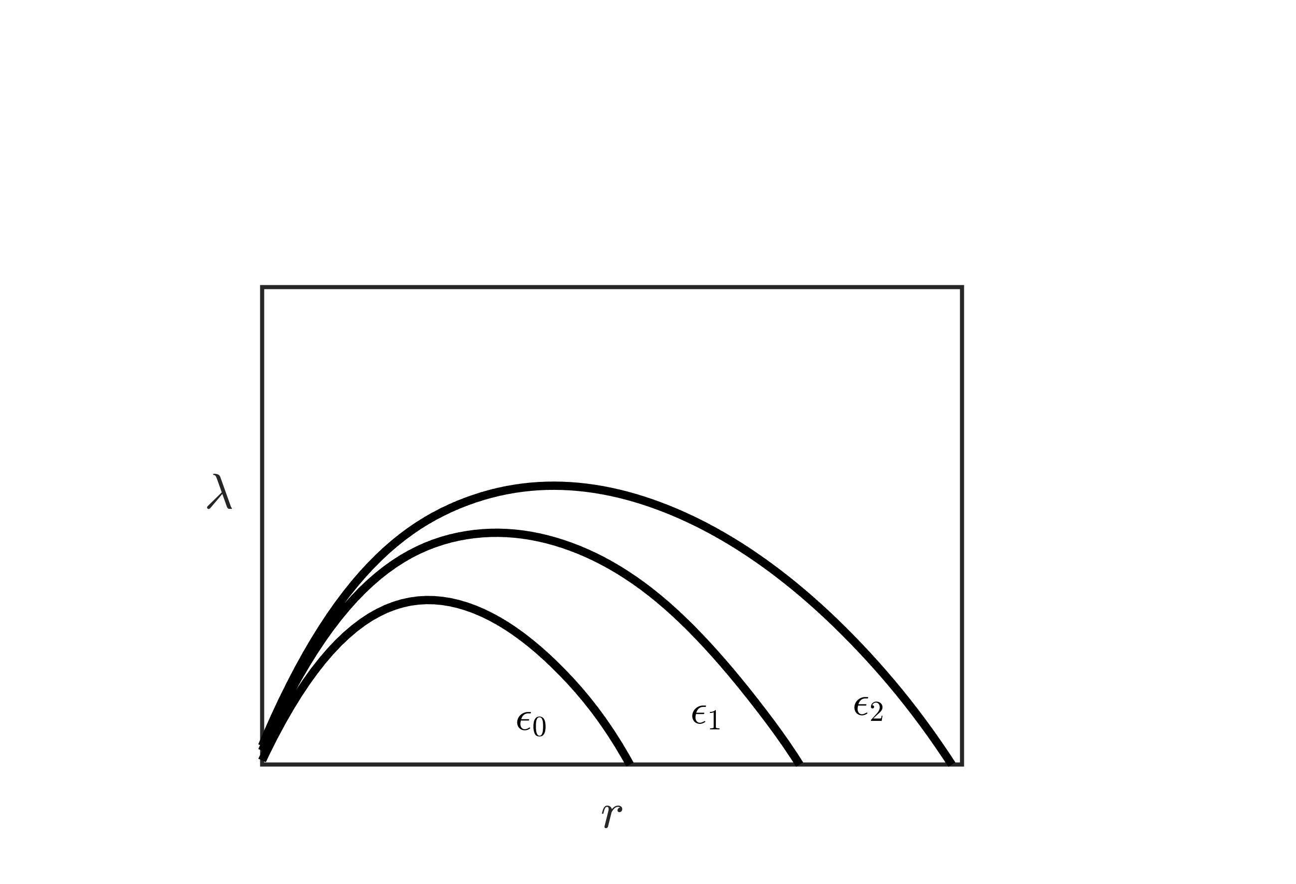
Figure 4: $\lambda$ vs $r$ for the TF potential.

As a further example of the behavior of $\lambda,$ consider the case of the Coulomb potential where we have

$$Z\,r_{l}=\frac{1\pm\sqrt{1-2\,\epsilon\,\lambda^{2}}}{2\,\epsilon},\text{where }\epsilon=-\varepsilon/Z^{2},$$

which yield two turning points except when $\nu=0$ and where $\lambda_{\varepsilon}(r)=\frac{Z}{\sqrt{2|\varepsilon|}}$ at which $r_{\varepsilon}=\frac{Z}{2\left|\varepsilon\right|}.$  In Fig. (5) we have plotted $\lambda_{\epsilon}=\sqrt{2\,\mathfrak{r}\,\left[1-\mathfrak{r}\,\epsilon\right]}$as a function of the scaled distance $\mathfrak{r}=Z\,r$ and the scaled energy $\epsilon$

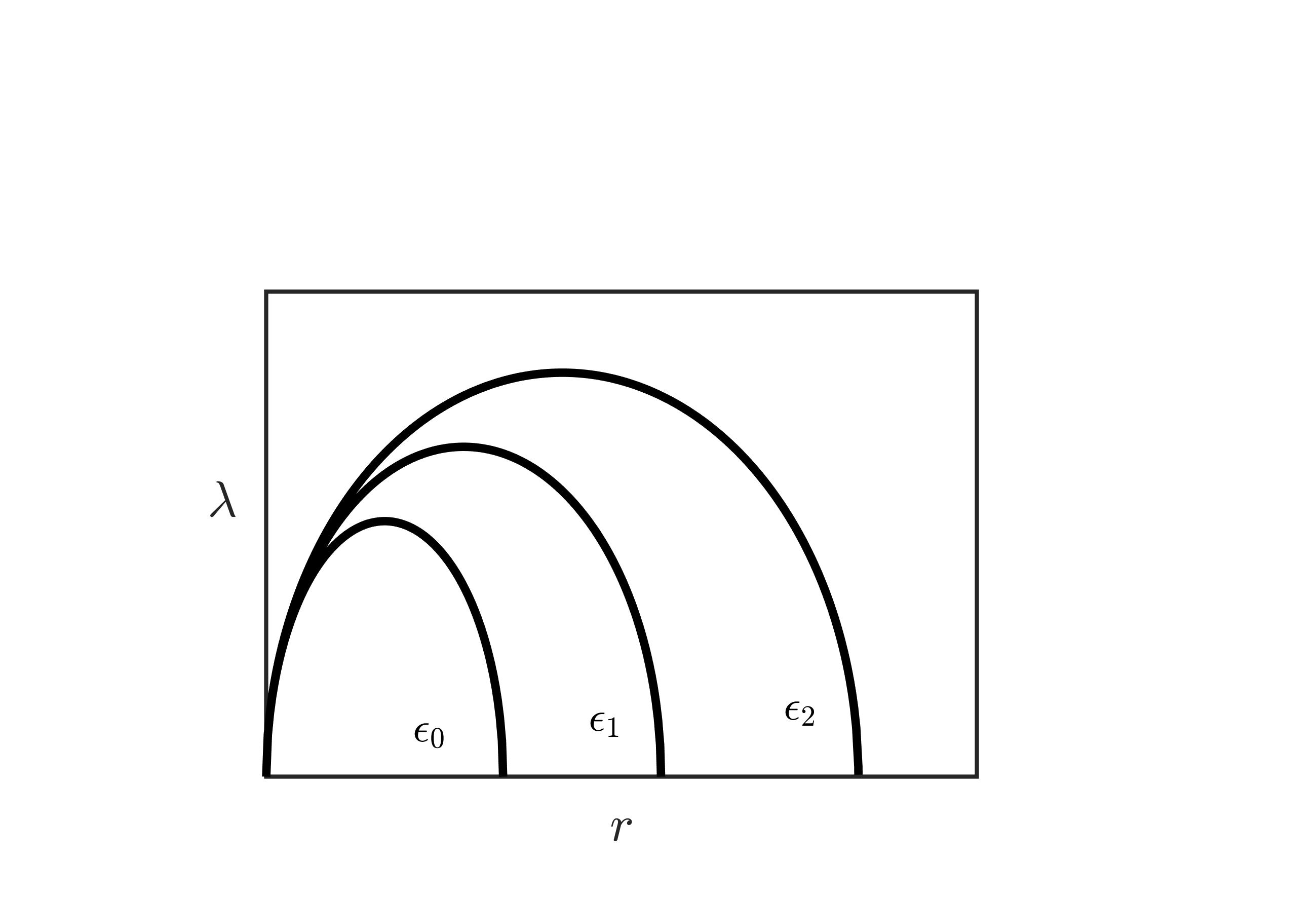
Figure 5: $\lambda$ vs $r$ for the Coulomb potential

We see in the case of the Coulomb potential for a given $\varepsilon$ with $\lambda_{\varepsilon}=0$, there is a set of classical turning points which occur at $0$ and $\frac{Z}{\left|\varepsilon\right|},$whereas the maximum values of $\lambda_{\varepsilon}$ are $\lambda_{\varepsilon,\max}(r)=\frac{Z}{\sqrt{2\left|\varepsilon\right|}}$, and the set of single turning points occur at $r_{\varepsilon,\max}=\frac{Z}{2\left|\varepsilon\right|}$.  Furthermore, for a given $\varepsilon(\lambda,\nu)=const$  the variables $\lambda$ and $\nu(\lambda|\varepsilon)$ are related as shown in the Fig. (6) below.

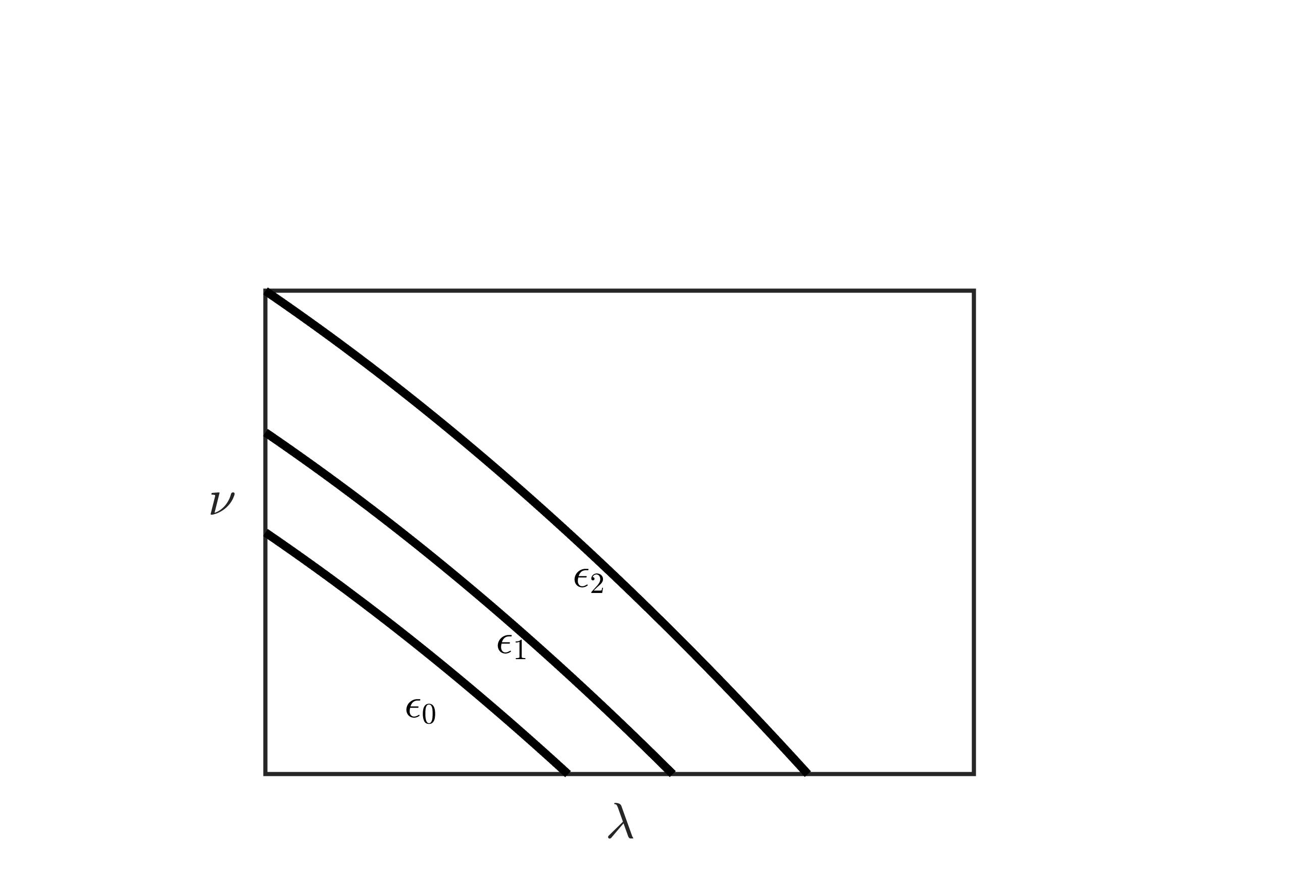
Figure 6: $\nu$ vs. $\lambda$ for the TF potential.

We expect the shape of the curves in Fig. 6 to show concave curvature as is the case of the TF potential.  Along these curves the energy is constant (curves of degeneracy).  In the case of the Coulombic potential, where the energy is $\varepsilon=-Z^{2}/2(\lambda+\nu)^{2}$ the curves in the plot of $\nu(\lambda|\varepsilon)$ versus $\lambda$ for different $\varepsilon$ consists of a family of straight lines whereas in the case of a general potential we expect these lines to be curved as shown above [16].  In addition we denote the maximum value of $\nu$ i.e. $\nu(0|\varepsilon)=\nu_{\varepsilon}.$  From this we see that for a given $\varepsilon$ the quantities $\lambda$ and $\nu$ are restricted to the ranges

$$0\leq\lambda\leq\lambda_{\varepsilon}(r),$$

$$0\leq\nu\leq\nu(\lambda|\varepsilon).$$

The domain of integration in $\lambda,\nu$ space is seen to consist of all $\lambda,\nu$ values below the curves of degeneracy $\nu(\lambda|\varepsilon)$ corresponding to $\varepsilon=\varepsilon_{0}$.  With this in mind we can for a given $\varepsilon$ rewrite the average potential $\overline{V}_{ne}$ as

$$\overline{V}_{ne}=4\lim_{\varepsilon\longrightarrow\varepsilon_{0}}\sum_{k=-\infty}^{\infty}\sum_{j=-\infty}^{\infty}(-1)^{k+j}\int_{0}^{\lambda_{\varepsilon}(r)}\lambda\exp(2\pi ik\lambda)\,d\lambda\int_{0}^{\nu(\lambda|\varepsilon)}\exp(2\pi ij\nu)\,{\large\upsilon}_{\lambda,\nu}\,d\nu,$$ (11)

with $\nu(\lambda|\varepsilon)$ denoting the curves of degeneracy.

In the work to follow it is useful to define the integrals $\mathcal{N}_{j}\,\mathcal{(}\lambda_{\varepsilon},\varepsilon_{\lambda,\nu})$ as

$$\mathcal{N}_{j}\mathcal{(}\lambda,\varepsilon)=\int_{0}^{\nu(\lambda|\varepsilon)}\cos(2\pi j\,\nu)\,{\large\upsilon}_{\lambda,\nu}\,\,d\nu.$$

1.4 The Regions Of $k,\,j$ Space

In order to make progress in evaluating the terms in the double sum in Eq. (11) for $\overline{V}_{ne}$ it is useful to divide $k,\,j$ index space (note that $\lambda$ and $\nu$ are associated with the indices $k,$ and $j$ respectively) into the regions shown in the diagram below.  These regions shown in Fig. (7) correspond roughly to those chosen by SE in their evaluation the energy of the system.

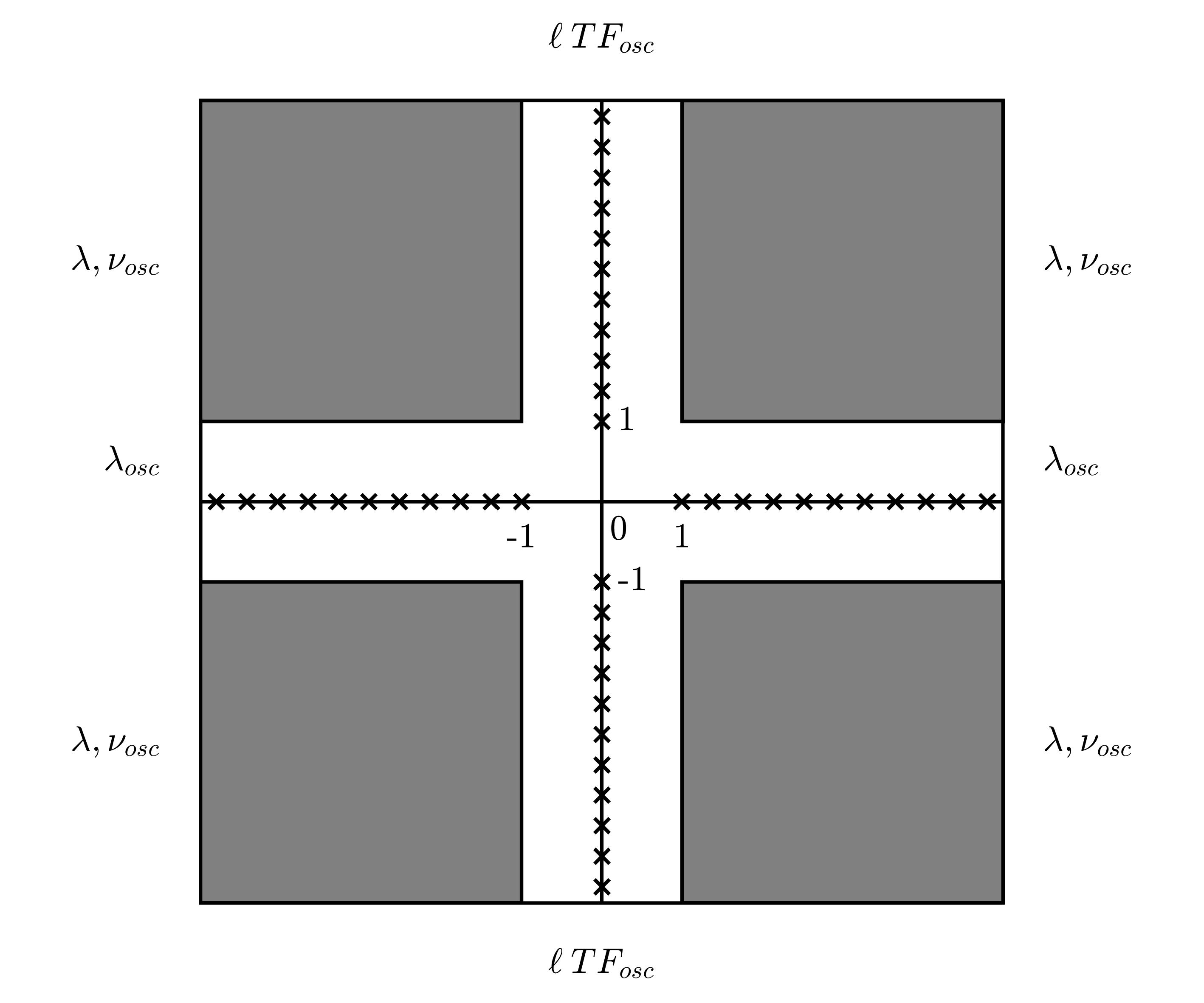
Figure 7: Regions within the $k,$ $j$ space.

The TF region consists of the single point

$$j=0,\hskip 10.84006ptk=0$$

the l TF region consists of the points on the vertical line

$$\text{\ }j=0,\hskip 18.06749pt1\leq k\leq\infty,$$

the $\lambda$ region is given by

$$k=0,\hskip 18.06749pt1\leq j\leq\infty\text{,}$$

and the $\lambda,\nu$ region consists of the points covered by the ranges

$$1\leq j\leq\infty,\text{ \ \ }1\leq k\leq\infty.$$

Rewriting $\overline{V}_{ne}$ in terms of these regions we have

$$\overline{V}_{ne}=\lim_{\varepsilon\rightarrow\varepsilon_{0}}\left\{\,\overline{V}_{ne,TF}(\varepsilon)+\overline{V}_{ne,lTF}(\varepsilon)+\overline{V}_{ne,\,\lambda}(\varepsilon)+\overline{V}_{ne,\,\,\lambda\mathbf{,}\nu}(\varepsilon)\,\right\},$$ (12)

where

$$\overline{V}_{ne,TF}(\varepsilon) =4\int_{0}^{\lambda_{\varepsilon}}\lambda\,\mathcal{N}_{0}\mathcal{(}\lambda,\varepsilon)\,d\lambda,$$ (13a)

$$\overline{V}_{ne,\,\mathit{l}TF}(\varepsilon) =8\sum_{k=1}^{\infty}(-1)^{k}\int_{0}^{\lambda_{\varepsilon}}\lambda\cos(2\pi k\lambda)\,\mathcal{N}_{0}\mathcal{(}\lambda,\varepsilon)\,d\lambda,$$ (13b)

$$\overline{V}_{ne,\,\lambda}(\varepsilon) =8\sum_{j=1}^{\infty}(-1)^{j}\int_{0}^{\lambda_{\varepsilon}}\lambda\,\mathcal{N}_{j}\mathcal{(}\lambda,\varepsilon)\,d\lambda$$ (13c)

$$\overline{V}_{ne,\,\,\lambda,\nu}(\varepsilon) =16\sum_{k=1}^{\infty}\sum_{j=1}^{\infty}(-1)^{k+j}\int_{0}^{\lambda_{\varepsilon}}\lambda\,\cos(2\pi k\lambda)\,\mathcal{N}_{j}\mathcal{(}\lambda,\varepsilon)\,d\lambda\,.$$ (13d)

The numerical factors appearing in Eqs (13) result from the contributions from the second, third and fourth quadrants of Fig. (7).  We will see below that the first term shown in (13) i.e. $$\overline{V}_{ne,TF} \overline{V}_{ne,\,\mathit{l}TF,\,} l- \lambda \lambda,\nu$$ produces a non-oscillatory, semiclassical expression for the average nuclear electronic potential.  The sum over the second region produces an oscillatory semiclassical expression which we will call the ‘ quantized’ semiclassical average potential.  Oscillatory terms in the remaining regions will be called the ‘, and the - quantized’  contributions to the average potential respectively.

1.5 Evaluation Of $\mathcal{N}_{j}\mathcal{(}\lambda_{\,},\varepsilon_{\lambda,\nu})=\int_{0}^{\nu(\lambda|\varepsilon)}\cos(2\pi\,j\nu)\,\,{\Huge\upsilon}_{\lambda,\nu}\,\,d\nu$

The program for the evaluation of the expression for $\overline{V}_{ne}$ in Eq. (12), is best carried out by investigating its various parts in a stepwise fashion in order to simplify the exposition of the work.  We begin by noting that (recall $\upsilon_{\lambda,\nu}=\overline{V}_{l\,,\,n_{r}},$)

$$-\frac{{\large\upsilon}_{\lambda,\nu}}{Z}=\int_{r_{l}}^{r_{u}}\frac{\left|u_{l,n_{r}}(r)\right|^{2}}{r}dr=\frac{\left|A_{\lambda,\nu}\right|^{2}}{2}\int_{r_{l}}^{r_{u}}\frac{dr}{r\sqrt{2\{\varepsilon_{\lambda,\nu}-V(r)-{\small\lambda}^{2}{\small/2}r^{2}\}}},$$ (14)

and

$$\int_{0}^{\infty}\left|u_{l,n_{r}}(r)\right|^{2}dr=1=\frac{\left|A_{\lambda,\nu}\right|^{2}}{2}\int_{r_{l}}^{r_{u}}\frac{dr}{\sqrt{2\{\varepsilon_{\lambda,\nu}-V(r)-{\small\lambda}^{2}{\small/2}r^{2}\}}}.$$

Differentiation of $\nu$ with respect to $\varepsilon$ in Eq. (8) gives

$$\left(\frac{\partial\nu}{\partial\varepsilon_{\lambda,\nu}}\right)|_{\lambda}=\frac{1}{\pi}\int_{r_{l}}^{r_{u}}\frac{dr}{\sqrt{2\{\varepsilon_{\lambda,\nu}-V(r)-{\small\lambda}^{2}{\small/2}r^{2}\}}},$$

and thus

$$\frac{\left|A_{\lambda,\nu}\right|^{2}}{2}=\frac{1}{\pi}\left(\frac{\partial\varepsilon_{\lambda,\nu}}{\partial\nu}\right)|_{\lambda}.$$

As a result we may rewrite Eq. (14) as (valid for all $\lambda$ and $\nu)$

$$-\frac{{\large\upsilon}_{\lambda,\nu}}{Z}=\frac{1}{\pi}\left(\frac{\partial\varepsilon_{\lambda,\nu}}{\partial\nu}\right)_{\lambda}\int_{r_{l}}^{r_{u}}\frac{dr}{\sqrt{2r^{2}\{\varepsilon_{\lambda,\nu}-V(r)\}-{\small\lambda}^{2}}}.$$

The integral $\mathcal{N}_{j}\mathcal{(}\lambda,\varepsilon)$ over the variable $\nu$ then becomes (for a given $\lambda$ the energy $\nu$ can vary with $\varepsilon$)

$$\mathcal{N}_{j}\mathcal{(}\lambda,\varepsilon)=-\frac{Z}{\pi}\int_{0}^{\nu(\lambda|\varepsilon)}d\nu\,\cos(2\pi j\nu)\,\left(\frac{\partial\varepsilon_{\lambda,\nu}}{\partial\nu}\right)_{\lambda}\int_{r_{l}}^{r_{u}}\frac{dr}{\sqrt{2r^{2}\{\varepsilon_{\lambda,\nu}-V(r)\}-{\small\lambda}^{2}}}.$$ (15)

Interchanging the order of integration we get

$$\mathcal{N}_{j}\mathcal{(}\lambda,\varepsilon)=-\frac{Z}{\pi}\int_{r_{l}}^{r_{u}}dr\int_{0}^{\nu(\lambda|\varepsilon)}d\nu\,\,\left(\frac{\partial\varepsilon_{\lambda,\nu}}{\partial\nu}\right)_{\lambda}\frac{\cos(2\pi j\nu)}{\sqrt{2r^{2}\{\varepsilon_{\lambda,\nu}-V(r)\}-{\small\lambda}^{2}}}.$$ (16)

If the relation

$$(\frac{\partial\varepsilon_{\lambda,\nu}}{\partial\nu})_{\lambda}\frac{\cos(2\pi j\nu)}{\sqrt{2r^{2}\{\varepsilon_{\lambda,\nu}-V(r)\}-{\small\lambda}^{2}}}$$

$$=2\pi j\sin(2\pi j\nu)\tfrac{\sqrt{2r^{2}\{\varepsilon_{\lambda,\nu}-V(r)\}-{\small\lambda}^{2}}}{r^{2}}+\frac{\partial}{\partial\nu}[\cos(2\pi j\nu)\tfrac{\sqrt{2r^{2}\{\varepsilon_{\lambda,\nu}-V(r)\}-{\small\lambda}^{2}}}{r^{2}}]_{\lambda},$$

is used, we get an expression for $\mathcal{N}_{j}\mathcal{(}\lambda,\varepsilon)$ which is partially integrable i.e.

$$\mathcal{N}_{j}\mathcal{(}\lambda,\varepsilon)$$

$$=-\frac{Z}{\pi}\int_{r_{l}}^{r_{u}}dr\int_{0}^{\nu(\lambda|\varepsilon)}\{2\pi j\sin(2\pi j\nu)\tfrac{\sqrt{2r^{2}\{\varepsilon_{\lambda,\nu}-V(r)\}-{\small\lambda}^{2}}}{r^{2}}+\frac{\partial}{\partial\nu}[\cos(2\pi j\nu)\tfrac{\sqrt{2r^{2}\{\varepsilon_{\lambda,\nu}-V(r)\}-{\small\lambda}^{2}}}{r^{2}}]_{\lambda}\}d\nu\,.$$

And finally we obtain

$$\mathcal{N}_{j}\mathcal{(}\lambda,\varepsilon) =-\frac{Z}{\pi}\int_{r_{l}}^{r_{u}}\frac{dr}{r^{2}}\cos(2\pi j\nu(\lambda|\varepsilon))\sqrt{2r^{2}\{\varepsilon_{\lambda,\nu(\lambda|\varepsilon)}-V(r)\}-{\small\lambda}^{2}}$$

$$-2Z\,j\int_{r_{l}}^{r_{u}}\frac{dr}{r^{2}}\int_{0}^{\nu(\lambda|\varepsilon)}\sin(2\pi j\nu)\sqrt{2r^{2}\{\varepsilon_{\lambda,\nu}-V(r)\}-{\small\lambda}^{2}}d\nu,$$

an expression which will be useful in the evaluation of the integrals in Eq. (12).

1.6 Thomas Fermi parameters $r_{0},$ $\lambda_{0},$ $\omega_{0},$ $\nu_{0}^{(1)},$ $\nu_{0}^{(2)},\mathcal{K}_{0}(r_{0})$

At this juncture it is useful to review Thomas-Fermi (TF) theory and to compute some of the parameters which will be needed in the final calculation of the chemical potential.  In TF theory the potential $V(r)$ is defined by the equations

$$\nabla^{2}V=-4\pi\varrho_{TF}(\mathbf{r}),$$

$$\varrho_{TF}(\mathbf{r})=\frac{1}{3\pi^{2}}\left(2\{\varepsilon_{0}-V(r)\}\right)^{3/2}.$$ (17)

In the case of a spherically symmetric system this equation can be rewritten as

$$\frac{d^{2}\Phi}{d\,x^{2}}=\frac{\Phi(x)^{3/2}}{\sqrt{x}},\qquad\text{with \ \thinspace}\Phi(0)=1,\text{ }\Phi(\infty)=0,$$

As seen above in the case of the Coulombic potential the value of $r$ at which $\lambda$  is a maximum for a given $\varepsilon$ had been given as

$$r_{\varepsilon}=\frac{Z}{2\left|\varepsilon\right|}.$$

Here using the TF potential we give the value of $r$ corresponding to the maximum of $\lambda$ in the case where $\varepsilon\rightarrow\varepsilon_{0}.$  Using Eq. (10) we have

$$\frac{d\,\lambda_{0}^{2}(r)}{d\,r}=0=\frac{d}{d\,r}\{-2r^{2}V(r)\},$$

which is tantamount to

$$\frac{d\{x\,\Phi(x)\}}{d\,x}=0.$$

The maximum of the quantity $x\,\Phi(x)$ occurs at $x_{0}=2.10403$ where $\Phi(x_{0})=0.231151$ the corresponding value of $r_{0}$ being $2.10403\,a/Z^{1/3}$ [17].  The largest of the maximum values of $\lambda_{\varepsilon}$ i.e. $\lambda_{0\text{ }}$is then

$$\lambda_{0\text{ }}(r_{0})=\sqrt{2a\,x_{0}\Phi(x_{0})}\,Z^{1/3}=0.927992\,Z^{1/3}.$$

In the work that follows a collection of quantities (which have been computed by Schwinger and Englert ) for the TF potential is given below and will prove useful in the estimation of the $Z$ dependence of the remaining terms in $\overline{V}_{ne}.$ We have

$x_{0}=2.10403,$ $r_{0}=1.86278\,Z^{-1/3},$ $\omega_{\varepsilon}^{2}=-\frac{d^{2}\lambda_{\varepsilon}^{2}(r)}{d\,r^{2}}|_{r=r_{\varepsilon}}$ $\omega_{0}=0.36359\,Z^{\,2/3},$ $\lambda_{0}(r_{0})=0.92799\,Z^{\,1/3},$ $\overset{\bullet}{\lambda}=\frac{\partial\lambda_{\varepsilon}(r_{0})}{\partial\varepsilon}|_{\varepsilon=0}=r_{0}^{2}/\lambda_{0}(r_{0})=3.73921Z$ $\frac{\lambda_{0}(r_{0})}{\overset{\bullet}{\lambda}}=\left(\frac{\lambda_{0}(r_{0})}{r_{0}}\right)^{2}=0.24818Z^{4/3}$ $\nu_{0}^{(1)}=-\frac{\partial\nu_{0}(\lambda)}{\partial\lambda}|_{\lambda=\lambda_{0}}=\sqrt{2}\frac{\lambda_{0}(r_{0})}{\omega_{0}r_{0}}=1.93768,$ $\nu_{0}^{(2)}=-\frac{\partial^{2}\nu_{0}(\lambda)}{\partial\lambda^{2}}|_{\lambda=\lambda_{0}}=\frac{\nu_{0}^{(1)}}{24\lambda_{0}(r_{0})}[(\nu_{0}^{(1)})^{2}-1][-15+23(\nu_{0}^{(1)})^{2}-5(\nu_{0}^{(1)})^{4}]=0.208673/Z^{1/3},$ $\frac{\omega_{0}^{2}}{\lambda_{0}(r_{0})}=0.14246\,Z$ $\mathcal{K}_{0}(r_{0})=\frac{\lambda_{0}^{2}(r_{0})}{Z\,r_{0}}=0.46230,$ $\frac{\lambda_{0}^{3}(x_{0})}{\omega_{0}r_{0}^{3}\,}=0.34004\,Z^{\,4/3},$     

1.7 The TF Term $\overline{V}_{ne,TF}$

In the case where  $j=0$ we have for $\mathcal{N}_{0}\mathcal{(}\lambda,\varepsilon_{\lambda,\nu(\lambda|\varepsilon)})$

$$\mathcal{N}_{0}\mathcal{(}\lambda,\varepsilon_{\lambda,\nu(\lambda|\varepsilon)})=-\frac{Z}{\pi}\int_{r_{l}}^{r_{u}}\frac{dr}{r^{2}}\sqrt{2r^{2}\{\varepsilon_{\lambda,\nu(\lambda|\varepsilon)}-V(r)\}-{\small\lambda}^{2}},$$ (18)

the corresponding value of $\overline{V}_{ne,TF}$ then becomes

$$\overline{V}_{ne,TF}(\varepsilon)=-\frac{4Z}{\pi}\int_{0}^{\lambda_{\varepsilon}}\lambda d\lambda\int_{r_{l}}^{r_{u}}\sqrt{2r^{2}\{\varepsilon_{\lambda,\nu(\lambda|\varepsilon)}-V(r)\}-{\small\lambda}^{2}}dr/r^{2}.$$

Interchanging the order of integration results in ($r_{l}\leq r\leq r_{u})$

$$\overline{V}_{ne,TF}(\varepsilon)=-\frac{4Z}{\pi}\int_{r_{l}}^{r_{u}}dr/r^{2}\int_{0}^{\lambda_{\varepsilon}}\lambda d\lambda\sqrt{2r^{2}\{\varepsilon_{\lambda,\nu(\lambda|\varepsilon)}-V(r)\}-\lambda^{2}},$$

and we note that as $\lambda$ varies over its range from $0$ to $\lambda_{\varepsilon}$ in the limit as $\varepsilon\rightarrow\varepsilon_{0}\rightarrow 0$ the turning points must vary from $r_{l}=0$ and $r_{u}=\infty$  these being the roots of $2r^{2}\{\varepsilon_{0}-V(r)\}-\lambda_{0}^{2}=0.$  Integration over $\lambda$ gives the result

$$\overline{V}_{ne,TF}=-\frac{4Z}{3\pi}\int_{0}^{\infty}\left(2r^{2}\{\varepsilon_{0}-V(r)\}\right)^{3/2}dr/r^{2}.$$ (19)

Remarkably, if $V(r)$ is taken to be the Thomas-Fermi potential, the corresponding particle density $\varrho_{TF}(\mathbf{r})$ with the form

$$\varrho_{TF}(\mathbf{r})=\frac{1}{3\pi^{2}}\left(2\{\varepsilon_{0}-V(r)\}\right)^{3/2},$$

then $\overline{V}_{ne,TF}$ in Eq. (19) rewritten as a integral over 3 dimensional space is just

$$\overline{V}_{ne,TF}=-Z\int\frac{\varrho_{TF}(\mathbf{r})}{r}\,d\mathbf{r}=\overline{V}_{TF}$$

We see that the leading term in the expression for $\overline{V}_{ne}$ is the non-oscillatory Thomas-Fermi average value of the nuclear-electronic interaction $\overline{V}_{TF}$.  The remaining terms in the sums in Eq. (12) represent the semi-classical and oscillatory contributions to the nuclear-electronic interaction.

1.8
The Term $\overline{V}_{ne\,,\mathit{\,l}TF}\,$ The $\mathit{l}$ TF Oscillations

The sum representing $\overline{V}_{ne\,,\mathit{\,l}TF}\,$ can be rewritten as

$$\overline{V}_{ne\,,\mathit{\,l}TF}\,(\varepsilon) =8\sum_{k=1}^{\infty}(-1)^{k}\int_{0}^{\lambda_{\varepsilon}}d\lambda\,\lambda\cos(2\pi ik\lambda)\int_{0}^{\nu_{\varepsilon}(\lambda)}\,{\large\upsilon}_{\lambda\,,\nu}\,d\nu$$

$$\overline{V}_{ne\,,\mathit{\,l}TF} =\lim_{\varepsilon\longrightarrow\varepsilon_{0}}\,\overline{V}_{ne\,,\mathit{\,l}TF}\,(\varepsilon)$$

Once again interchange of the order of integration in the integrals above and use of the procedure to obtained $\overline{V}_{TF}$ (with the expression for $\mathcal{N}_{0}\mathcal{(}\lambda,\varepsilon_{\lambda,\nu(\lambda|\varepsilon)})$ in Eq. (18) $\overline{V}_{ne\,,\,lTF}\,(\varepsilon)$ can then be rewritten as

$$\overline{V}_{ne\,,\mathit{\,l}TF}\,(\varepsilon)=-\,\frac{8Z}{\pi}\sum_{k=1}^{\infty}(-1)^{k}\int_{r_{l}}^{r_{u}}\frac{dr}{r^{2}}\int_{0}^{\lambda_{\varepsilon}}d\lambda\cdot\lambda\cos(2\pi ik\lambda)\sqrt{2r^{2}\{\varepsilon_{\lambda_{\varepsilon}},_{{\large\nu}(\lambda|\varepsilon)}-V(r)\}-\lambda^{2}}.$$

Now we write

$$\lambda_{\varepsilon}^{2}=2r^{2}\{\varepsilon_{\lambda_{\varepsilon}},_{\nu(\lambda|\varepsilon)}-V(r)\},$$

and $\lambda$ as

$$\lambda=\lambda_{\varepsilon}(r)\cos\theta,\text{ \hskip 18.06749pt}0\leq\theta\leq\pi/2.$$

The expression for $\overline{V}_{ne\,,\mathit{\,l}TF}\,(\varepsilon)$ with this change of variable becomes

$$\overline{V}_{ne\,,\mathit{\,l}TF}\,(\varepsilon)=-\frac{8Z}{\pi}\sum_{k=1}^{\infty}(-1)^{k}\int_{r_{l}}^{r_{u}}\frac{\lambda_{\varepsilon}^{3}(r)}{r^{2}}dr\int_{0}^{\pi/2}\sin^{2}\theta\cos\theta\cos(2\pi k\lambda_{\varepsilon}(r)\cos\theta)\,d\theta.$$

The angular integral appearing in the equation above is well-known and we have

$$\int_{0}^{\pi/2}\sin^{2}\theta\cos\theta\cos(2\pi k\lambda_{\varepsilon}\cos\theta)\,d\theta=\frac{1}{3}-\frac{\pi\mathbf{H}_{2}(2\pi k\lambda_{\varepsilon})}{4\pi\,k\,\lambda_{\varepsilon}},$$

where $\mathbf{H}_{2}(z)$ are the Struve functions [18] of order $2$.  The required sum is then

$$\overline{V}_{ne\,,\mathit{\,l}TF}\,(\varepsilon)=-\frac{8Z}{\pi}\sum_{k=1}^{\infty}(-1)^{k}\int_{r_{l}}^{r_{u}}\frac{\lambda_{\varepsilon}^{3}(r)}{r^{2}}\left[\frac{1}{3}-\frac{\pi\mathbf{H}_{2}(2\pi k\lambda_{\varepsilon}(r))}{4\pi\,k\,\lambda_{\varepsilon}(r)}\right]\,dr.$$

In the case of integer order, the Struve functions $\mathbf{H}_{k}(z)$ are related to the Weber functions $\mathbf{E}_{k}(z)$ [19] .  In this case

$$\frac{1}{3}-\frac{\pi}{2z}\mathbf{H}_{2}(z)=\frac{\pi}{2z}\mathbf{E}_{2}(z),$$

and we can write within the semiclassical approximation an exact expression for$\overline{V}_{ne\,,\mathit{\,l}TF}\,(\varepsilon)$ as

$$\overline{V}_{ne\,,\mathit{\,l}TF}\,(\varepsilon)=-\frac{2Z}{\pi}\sum_{k=1}^{\infty}\frac{(-1)^{k}}{k}\int_{r_{l}}^{r_{u}}\frac{\lambda_{\varepsilon}^{2}(r)}{\,\,\,r^{2}}\mathbf{E}_{2}(2\pi k\lambda_{\varepsilon}(r))dr.$$

For the Thomas-Fermi function $\Phi(x)$ where $\varepsilon=-\,\varsigma=0$ we note that

$$\lambda_{0}(r)=Z^{1/3}\sqrt{2a\,x_{0}\,\Phi(x_{0})},$$

and see that for large $Z,$ that $\lambda_{0}(r)$ is large.  For large $Z,$ using the asymptotic expansion for the leading and next to leading terms [20] for $\mathbf{E}_{2}(z)$ i.e.

$$\frac{\pi}{2z}\mathbf{E}_{2}(z)\thicksim\sqrt{\frac{\pi}{2}}\frac{1}{z^{3/2}}\left\{-\cos(z+\pi/4)+\frac{15}{8z}\sin(z+\pi/4)\right\},$$

the integral to be evaluated is

$$\int_{r_{l}}^{r_{u}}\frac{\lambda_{\varepsilon}^{2}(r)}{\,\,\,r^{2}}\mathbf{E}_{2}(2\pi k\lambda_{\varepsilon}(r))dr=$$

$$-\frac{1}{\pi k^{1/2}}\int_{0}^{\infty}\frac{\lambda_{\varepsilon}^{3/2}(r)}{\,\,\,r^{2}}\left\{\cos(2\pi k\lambda_{\varepsilon}(r)+\pi/4)-\frac{15}{16\pi k\lambda_{\varepsilon}(r)}\sin(2\pi k\lambda_{\varepsilon}(r)+\pi/4)\right\}dr.$$

As stated in the SE paper we are not interested in the detailed content in this quantity, but instead only in the leading oscillatory contributions to it.  Evaluation of this integral for large $\lambda_{\varepsilon}$ can be obtained using the ‘stationary phase approximation.’[21]  Recalling that $\lambda_{{}_{\varepsilon}}(r)$ has a maximum at the point $r_{{}_{\varepsilon}}$ expansion of that function around $r_{{}_{\varepsilon}}$ gives

$$\lambda_{{}_{\varepsilon}}(r)=\lambda_{{}_{\varepsilon}}(r_{\varepsilon})-\tfrac{1}{4}\tfrac{\omega_{{}_{\varepsilon}}^{2}}{\lambda_{{}_{\varepsilon}}(r_{{}_{\varepsilon}})}(r-r_{{}_{\varepsilon}})^{2}+\ldots,$$

where $\omega_{0}^{2}/\lambda_{0}(r_{0})$ is proportional to $Z$ and is large.  In the limit as $\varepsilon\rightarrow\varepsilon_{0}$ and within that approximation the leading oscillatory terms for the average potential $\overline{V}_{ne,\,\mathit{l}TF}$ is

$$-\frac{\overline{V}_{ne\,,\mathit{\,l}TF}}{{\small Z}}\,={\small 2}\sqrt{{\small 2}}\frac{\,\lambda_{0}^{2}(r_{0})}{\omega_{0\,}r_{0}^{2}}\left[\sum_{k=1}^{\infty}\frac{(-1)^{k}}{\left(\pi k\right)^{2}}\cos({\small 2\pi}k\lambda_{0}{\small(r}_{0}{\small)})-\frac{15}{16\lambda_{0}}\sum_{k=1}^{\infty}\frac{(-1)^{k}}{\left(\pi k\right)^{3}}\sin({\small 2\pi}k\lambda_{0}{\small(r}_{0}{\small)})\right].$$

In the equation appearing above, sums of the kind

$$S_{n}(z) =\sum_{k=1}^{\infty}\frac{(-1)^{k}}{(\pi k)^{2n+1}}\sin(2\pi k\,z),$$

$$C_{n}(z) =\sum_{k=1}^{\infty}\frac{(-1)^{k}}{(\pi k)^{2n}}\cos(2\pi k\,z),$$

occur.  These infinite sums can be rewritten [22] in closed-form in terms of the periodic function $\left\langle z\right\rangle$ def ined by

$$\left\langle z\right\rangle=z-\lfloor z+1/2\rfloor\,,\hskip 36.135pt-\frac{1}{2}\leq\left\langle z\right\rangle<\frac{1}{2},$$

where $\lfloor z\rfloor\,$ is the floor function.  The f irst few of these sums are given here as

$$S_{0}(z) =-\,\left\langle z\right\rangle,$$

$$C_{1}(z) =\left\langle z\right\rangle^{2}-\tfrac{1}{12},$$

$$S_{1}(z) =\tfrac{2}{3}\left\langle z\right\rangle[\left\langle z\right\rangle^{2}-\tfrac{1}{4}],$$

$$C_{2}(z) =\tfrac{1}{90}-\tfrac{1}{3}[\left\langle z\right\rangle^{2}-\tfrac{1}{4}]^{2}.$$

The leading terms in the potential energy $\overline{V}_{ne,\,\mathit{l}TF}/{\small Z}$ written in terms of the closed-form expressions becomes

$$-\frac{\overline{V}_{ne,\,\mathit{l}TF}}{{\small Z}}={\small 2}\sqrt{{\small 2}}\frac{\,\lambda_{0}^{2}(r_{0})}{\omega_{0\,}r_{0}^{2}}\left[C_{1}(\lambda_{0}{\small)}-\frac{15}{16\lambda_{0}(r_{0})}S_{1}(\lambda_{0}{\small)}\right],$$ (20)

with

$$\frac{\,\lambda_{0}^{2}(r_{0})}{\omega_{0\,}r_{0}^{2}}=0.68258Z^{\,2/3}.$$

The $\mathit{l}TF$ contribution is seen to contain terms of orders $Z^{2/3}$ and $Z^{1/3}$.

1.9
The $\overline{V}_{ne,\lambda}$ and $\overline{V}_{ne,\lambda\,,\nu\,}$  Oscillations

The terms $\overline{V}_{ne,\lambda\,}$ and $\overline{V}_{ne,\lambda,\nu\,}$ are more complex in nature.  In those cases the integrals $\mathcal{N}_{j}\mathcal{(}\lambda,\varepsilon_{\lambda,\nu})$ with $j>0$ are complicated by the presence of the variable $\nu$ and trigonometric terms thereby requiring a more elaborate analysis.  Using the bounds defined by the appropriate regions of integration for $\lambda,\,\nu$ we have

$$\overline{V}_{ne,\,\lambda}(\varepsilon) =8\sum_{j=1}^{\infty}(-1)^{j}\int_{0}^{\lambda_{\varepsilon}}\lambda\,\mathcal{N}_{j}\mathcal{(}\lambda,\varepsilon_{\lambda,\nu})\,d\lambda$$ (21a)

$$\overline{V}_{ne,\lambda,\nu\,}(\varepsilon) =16\sum_{k=1}^{\infty}\sum_{j=1}^{\infty}(-1)^{k+j}\int_{0}^{\lambda_{\varepsilon}}\lambda\,\cos(2\pi k\lambda)\mathcal{N}_{j}\mathcal{(}\lambda,\varepsilon_{\lambda,\nu})\,d\lambda\,\,,$$ (21b)

where the $$\lambda,\, \lambda,\nu k=0, 1\leq j\leq\infty 1\leq j\leq\infty, \ \ 1\leq k\leq\infty$$and the region has been divided into the two, subregions def ined by and , respectively.

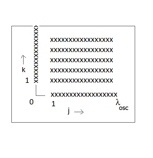
Figure 8: The $k$ vs. $j$ regions of summation

1.9.1 The Term $\mathcal{N}_{j}\mathcal{(}\lambda,\varepsilon_{\lambda,\nu})$ For $j\geq 1$ The $\lambda$ Oscillations

We have seen that $\mathcal{N}_{j}\mathcal{(}\lambda,\varepsilon_{\lambda,\nu})$ has been partially integrated with respect to $\nu$ i.e.

$$\mathcal{N}_{j}\mathcal{(}\lambda,\varepsilon_{\lambda,\nu}) =-\frac{Z}{\pi}\int_{r_{l}}^{r_{u}}\frac{dr}{r^{2}}\cos(2\pi j\nu(\lambda|\varepsilon))I_{0}(\nu(\lambda|\varepsilon),r,\lambda)$$

$$- 2Z\,j\int_{r_{l}}^{r_{u}}\frac{dr}{r^{2}}\int_{0}^{\nu(\lambda|\varepsilon)}\sin(2\pi j\nu)\,I_{0}(\nu,r,\lambda)\,d\nu{\small,}$$

where

$$I_{0}(\nu,r,\lambda)=\sqrt{2r^{2}\{\varepsilon_{\lambda,\nu}-V(r)\}-{\small\lambda}^{2}}.$$

The quantity $I_{0}(\nu,\lambda,r)$ evaluated at $\nu(\lambda|\varepsilon)$ simplifies and we get

$$I_{0}(\nu(\lambda|\varepsilon),\lambda,r) =\sqrt{2r^{2}\{\varepsilon_{\lambda,\nu(\lambda|\varepsilon)}-V(r)\}-\lambda^{2}}=\sqrt{\lambda_{\varepsilon}^{2}(r)-\lambda^{2}},$$

$$I_{0}(\nu(\lambda|\varepsilon),\lambda,r) =\lambda_{\varepsilon}(r)\sin\theta.$$

Integration by parts of the integral with respect to $\nu$ gives

$$\mathcal{N}_{j}\mathcal{(}\lambda,\varepsilon_{\lambda,\nu})=-\frac{Z}{\pi}\{\int_{r_{l}}^{r_{u}}\frac{dr}{r^{2}}\cos(2\pi j\nu(\lambda|\varepsilon))\,I_{0}(\nu(\lambda|\varepsilon),r,\lambda)$$

$$+2\pi j\int_{r_{l}}^{r_{u}}\frac{dr}{r^{2}}[\sin(2\pi j\nu(\lambda|\varepsilon)I_{1}(\nu(\lambda|\varepsilon),\lambda,r)-2\pi j\int_{0}^{\nu(\lambda|\varepsilon)}\cos(2\pi j\nu(\lambda|\varepsilon))I_{1}(\nu(\lambda|\varepsilon),\lambda,r)d\nu]\},$$

where

$$I_{1}(\nu(\lambda|\varepsilon),\lambda,r)=\int_{0}^{\nu(\lambda|\varepsilon)}I_{0}(\nu(\lambda|\varepsilon),\lambda,r)\,d\nu.$$

This process can be continued and the integral with respect to $\nu$ in the equation above can be integrated by parts once more to yield

$$\mathcal{N}_{j}\mathcal{(}\lambda,\varepsilon_{\lambda,\nu}) =-\frac{Z}{\pi}\{\int_{r_{l}}^{r_{u}}\frac{dr}{r^{2}}\cos(2\pi j\nu(\lambda|\varepsilon))I_{0}(\nu(\lambda|\varepsilon),\lambda,r)$$

$$+\left(2\pi j\right)\int_{r_{l}}^{r_{u}}\frac{dr}{r^{2}}\sin(2\pi j\nu(\lambda|\varepsilon))I_{1}(\nu(\lambda|\varepsilon),\lambda,r)$$

$$-(2\pi j)^{2}\int_{r_{l}}^{r_{u}}\frac{dr}{r^{2}}\cos(2\pi j\nu(\lambda|\varepsilon))I_{2}(\nu(\lambda|\varepsilon),\lambda,r)$$

$$-(2\pi j)^{3}\int_{r_{l}}^{r_{u}}\frac{dr}{r^{2}}\int_{0}^{\nu(\lambda|\varepsilon)}\sin(2\pi j\nu)I_{2}(\nu,\lambda,r)d\nu\},$$

where

$$I_{2}(\nu(\lambda|\varepsilon),\lambda,r)=\int_{0}^{\nu(\lambda|\varepsilon)}I_{1}(\nu(\lambda|\varepsilon),\lambda,r)\,d\nu.$$

The process introduced above can in principle be continued indefinitely however, it suff ices to terminate the expression for $\mathcal{N}_{j}\mathcal{(}\lambda,\varepsilon_{\lambda,\nu})$ at order $j^{\,2}$.

The integrals $I_{1}(\nu(\lambda|\varepsilon),\lambda,r)$ and $I_{2}(\nu(\lambda|\varepsilon),\lambda,r)$ have been approximately evaluated in appendix A and are given here by

$$\frac{I_{1}(\nu(\lambda|\varepsilon),\lambda,r)}{Zr}=\frac{\lambda_{\varepsilon}(r)}{Zr}\sqrt{\lambda_{\varepsilon}^{2}-\lambda^{2}}-\arctan(\frac{\lambda_{\varepsilon}(r)}{Zr}\sqrt{\lambda_{\varepsilon}(r)-\lambda^{2}}),$$

or in terms of the angular variable $\theta$

$$\frac{I_{1}(\nu(\lambda|\varepsilon),\lambda,r)}{Zr} =\mathcal{K}_{\varepsilon}\sin\theta-\arctan(\mathcal{K}_{\varepsilon}\sin\theta),$$

$$=\left[\mathcal{K}_{\varepsilon}\sin\theta\right]^{3}\,\mathcal{I}_{1}(\mathcal{K}_{\varepsilon}\sin\theta),$$

where $\mathcal{I}_{1}(z)$ is

$$\mathcal{I}_{1}(z) =\sum_{\kappa=0}^{\infty}\frac{(-1)^{\kappa}\,z^{2\kappa}}{\left(2\kappa+3\right)},\hskip 18.06749pt\left|z\right|\leq 1$$

$$\mathcal{I}_{1}(z) =\frac{1}{3}-\frac{z^{2}}{5}+\frac{z^{4}}{7}+\cdots,$$

and $\mathcal{K}_{0}$ is the unit less constant

$$\mathcal{K}_{0}=\frac{\lambda_{0}^{2}(r_{0})}{Z\,r_{0}}=0.46230.$$

Then

$$\frac{I_{1}(\nu(\lambda|\varepsilon),\lambda,r)}{Zr}=\frac{1}{3}\left[\mathcal{K}_{\varepsilon}\sin\theta\right]^{3}-\frac{1}{5}[\mathcal{K}_{\varepsilon}\sin\theta]^{5}+\cdots$$

Similarly we have

$$\frac{I_{2}(\nu(\lambda|\varepsilon),\lambda,r)}{2Zr\lambda_{\varepsilon}(r)} =\frac{\lambda_{\varepsilon}(r)}{Zr}\sqrt{\lambda_{\varepsilon}(r)^{2}-\lambda^{2}}-2\arctan(\frac{\lambda_{\varepsilon}(r)}{Zr}\sqrt{\lambda_{\varepsilon}(r)^{2}-\lambda^{2}})$$

$$+\frac{\arcsin h(\frac{\lambda_{\varepsilon}(r)}{Zr}\sqrt{\lambda_{\varepsilon}(r)^{2}-\lambda^{2}})}{\sqrt{1+\left(\frac{\lambda_{\varepsilon}(r)}{Zr}\right)^{2}(\lambda_{\varepsilon}(r)^{2}-\lambda^{2})}},$$

or in terms of $\theta$ we have

$$\frac{I_{2}(\nu(\lambda|\varepsilon),\lambda,r)}{2rZ\,\lambda_{\varepsilon}(r)} =\mathcal{K}_{\varepsilon}\sin(\theta)-2\arctan(\mathcal{K}_{\varepsilon}\sin\theta)+\frac{\arcsin h(\mathcal{K}_{\varepsilon}\sin\theta)}{\sqrt{1+\mathcal{K}_{\varepsilon}^{2}\sin^{2}\theta}},$$

$$=\left[\mathcal{K}_{\varepsilon}\sin\theta\right]^{5}\,\mathcal{I}_{2}(\mathcal{K}_{\varepsilon}\sin\theta),$$

where $\mathcal{I}_{2}(z)$ is

$$\mathcal{I}_{2}(z) =\sum_{\kappa=0}^{\infty}{\Large[}\Gamma(\kappa+5/2)-\tfrac{\sqrt{\pi}}{2}\Gamma(\kappa+3){\Large]}\tfrac{(-1)^{k}\,z^{2\kappa}}{\Gamma(\kappa+7/2)},\hskip 18.06749pt\left|z\right|\leq 1$$

$$\,\mathcal{I}_{2}(z) =\tfrac{2}{15}-\tfrac{6}{35}z^{2}+\tfrac{58}{315}z^{4}-\tfrac{130}{693}z^{6}+\,\cdots.$$

Finally

$$\frac{I_{2}(\nu(\lambda|\varepsilon),\lambda,r)}{2rZ\lambda_{\varepsilon}(r)}=\tfrac{2}{15}\left[\mathcal{K}_{\varepsilon}(r_{\varepsilon})\sin\theta\right]^{5}-\tfrac{6}{35}\left[\mathcal{K}_{\varepsilon}(r_{\varepsilon})\sin\theta\right]^{7}+\cdots.$$

We note that the integral $I_{2}$ is small compared to $I_{1}$ and will be dropped.

The integrals in $\overline{V}_{ne,\,\lambda}(\varepsilon)$ and $\overline{V}_{ne,\,\lambda,\nu}(\varepsilon)$ can then be written as

$$\overline{V}_{ne\lambda;\lambda,\nu\,} =\lim_{\varepsilon\rightarrow 0}\,\left[\overline{V}_{ne,\,\lambda}(\varepsilon)+\overline{V}_{ne,\,\lambda,\nu}(\varepsilon)\right]$$

$$=\left\{8\sum_{j=1}^{\infty}(-1)^{\,j}\,\mathcal{V}_{0}(\,j)+16\sum_{k=1}^{\infty}\sum_{j=1}^{\infty}(-1)^{k+j}\mathcal{V}_{1}(\,j,k)\,\right\}.$$ (22)

The $\mathcal{V}_{0}(\,j)$ integrals contain the $\lambda$ oscillation  terms and the $\mathcal{V}_{1}(\,j,k)$ terms contain the mixed $\lambda,\nu$ oscillation terms.  Now we get the expressions

$$\mathcal{V}_{0}(\,j) =-\frac{Z}{\pi}\{\int_{r_{l}}^{r_{u}}\frac{dr}{r^{2}}\int_{0}^{\lambda_{\varepsilon}}\lambda\,I_{0}(\nu(\lambda|\varepsilon))\cos(2\pi j\,\nu(\lambda|\varepsilon))d\lambda$$

$$+2\pi j\,\int_{r_{l}}^{r_{u}}\frac{dr}{r^{2}}\int_{0}^{\lambda_{\varepsilon}}\lambda\,I_{1}(\nu(\lambda|\varepsilon))\sin(2\pi j\,\nu(\lambda|\varepsilon))d\lambda\},$$

$$\mathcal{V}_{1}(\,j,k) =-\frac{Z}{\pi}\{\int_{r_{l}}^{r_{u}}\frac{dr}{r^{2}}\int_{0}^{\lambda_{\varepsilon}}\lambda\,I_{0}(\nu(\lambda|\varepsilon))\cos(2\pi k\lambda)\cos(2\pi j\,\nu(\lambda|\varepsilon))d\lambda\,$$

$$+2\pi j\int_{r_{l}}^{r_{u}}\frac{dr}{r^{2}}\int_{0}^{\lambda_{\varepsilon}}\,\lambda I_{1}(\nu(\lambda|\varepsilon))\cos(2\pi k\lambda)\sin(2\pi j\,\nu(\lambda|\varepsilon))\,d\lambda\}.$$

In the equations above we have interchange the order of integration over $r$ and $\lambda$ and used $\lambda=\lambda_{\varepsilon}\cos\theta$ where $0\leq\theta$ $\leq\pi/2$. to give

$$\mathcal{V}_{0}(\,j) =-\frac{Z}{\pi}\{\int_{r_{l}}^{r_{u}}\frac{\lambda_{\varepsilon}^{3}(r)}{r^{2}}\int_{0}^{\pi/2}\sin^{2}\theta\cos\theta\cos(2\pi j\,\nu(\lambda|\varepsilon))d\theta dr$$ (23)

$$+\frac{2\pi j}{Z^{2}}\,\int_{r_{l}}^{r_{u}}\frac{\lambda_{\varepsilon}^{8}(r)}{r^{4}}\int_{0}^{\pi/2}\,\sin^{4}\theta\cos\theta\sin(2\pi j\,\nu(\lambda|\varepsilon))\,\mathcal{I}_{1}(\mathcal{K}_{\varepsilon}\sin\theta)d\theta dr\},$$

$$\mathcal{V}_{1}(\,j,k) =-\frac{Z}{\pi}\{\int_{r_{l}}^{r_{u}}\frac{\lambda_{\varepsilon}^{3}(r)}{r^{2}}\int_{0}^{\pi/2}\sin^{2}\theta\cos\theta\cos(2\pi k\lambda_{\varepsilon}\cos\theta)\cos(2\pi j\,\nu(\lambda|\varepsilon))d\theta dr\,$$ (24b)

$$+\frac{2\pi j}{Z^{2}}\int_{r_{l}}^{r_{u}}\frac{\lambda_{\varepsilon}^{8}(r)}{r^{4}}\int_{0}^{\pi/2}\sin^{4}\theta\cos\theta\,\cos(2\pi k\lambda_{\varepsilon}\cos\theta)\sin(2\pi j\,\nu(\lambda|\varepsilon))\mathcal{I}_{1}(\mathcal{K}_{\varepsilon}\sin\theta)d\theta dr\,\}.$$

Written in more compact form the Eqs. (24) became

$$\mathcal{V}_{0}(\,j) =-\frac{Z}{\pi}\left\{\int_{r_{l}}^{r_{u}}\frac{\lambda_{\varepsilon}^{3}(r)\,}{r^{2}}\mathcal{C}_{0}^{\,\left(1\right)}(b,z,\varrho)\,dr+\frac{2\pi j}{Z^{2}}\int_{r_{l}}^{r_{u}}\frac{\lambda_{\varepsilon}^{8}(r)}{r^{4}}\mathcal{C}_{0}^{\,\left(2\right)}(\mathcal{K}_{\varepsilon},b,z,\varrho)\,dr\right\},$$

$$\mathcal{V}_{1}(\,j,k) =-\frac{Z}{\pi}\left\{\int_{r_{l}}^{r_{u}}\frac{\lambda_{\varepsilon}^{3}(r)}{r^{2}}\mathcal{C}_{1}^{\,\left(1\right)}(b,z,z^{\prime},\varrho)\,dr+\frac{2\pi j}{Z^{2}}\int_{r_{l}}^{r_{u}}\frac{\lambda_{\varepsilon}^{8}(r)}{r^{4}}\mathcal{C}_{1}^{\,\left(\,2\right)}(\mathcal{K}_{\varepsilon},b,z,z^{\prime},\varrho))\,dr\right\},$$

where the angular integrals are defined by

$$C_{0}^{\,\,\left(1\right)}(b,z,\varrho) =\int_{0}^{\pi/2}\sin^{2}\theta\cos\theta\cos(2\pi j\,\nu(\lambda|\varepsilon))\,d\theta,$$

$$C_{1}^{\,\,\left(1\right)}(b,z,z^{\prime},\varrho) =\int_{0}^{\pi/2}\sin^{2}\theta\cos\theta\cos(2\pi k\lambda_{\varepsilon}\cos\theta)\cos(2\pi j\,\nu(\lambda|\varepsilon))\,d\theta,$$

$$C_{0}^{\,\,\left(2\right)}(\mathcal{K}_{\varepsilon},b,z,\varrho) =\int_{0}^{\pi/2}\sin^{4}\theta\cos\theta\,\sin(2\pi j\,\nu(\lambda|\varepsilon))\,\mathcal{I}_{1}(\mathcal{K}_{\varepsilon}\sin\theta)\,d\theta,$$

$$C_{1}^{\,\left(\,2\right)}(\mathcal{K}_{\varepsilon},b,z,z^{\prime},\varrho) =\int_{0}^{\pi/2}\sin^{4}\theta\cos\theta\,\cos(2\pi k\lambda_{\varepsilon}\cos\theta)\sin(2\pi j\,\nu(\lambda|\varepsilon))\,\mathcal{I}_{1}(\mathcal{K}_{\varepsilon}\sin\theta)\,d\theta,$$

As will be seen below these angular integrals are complicated in that they contain the functions $\cos(2\pi j\,\nu(\lambda|\varepsilon))$, and $\cos(2\pi k\lambda_{\varepsilon}\cos\theta)\cos(2\pi j\,\nu(\lambda|\varepsilon))$ as well as their $\sin$ counterparts, quantities which are functions of $\theta$ as well as $\lambda_{\varepsilon}(r)$.  In order to make progress in evaluating these integrals which contain the term $\nu(\lambda|\varepsilon)$, we will expand that quantity as follows. Taking into account the fact that the $\nu(\lambda|\varepsilon)$ versus $\lambda$ curves show curvature, the Thomas Fermi lines of nonlinear degeneracy will be replaced by a quadratic polynomial with the choice of parameters used by SE (in SE’s notation $\nu_{\varepsilon}^{\,(1)}=\nu_{\varepsilon}^{\prime\,\text{\ }},$ and $\nu_{\varepsilon}^{\,(2)}=\nu_{\varepsilon}^{\,{}^{\prime\prime}})$ that is we write

$$\nu(\lambda|\varepsilon)=\nu_{\varepsilon}^{\,(1)}\,[\lambda_{\varepsilon}(r)-\lambda]-\tfrac{1}{2}\nu_{\varepsilon}^{\,(2)}\,[\lambda_{\varepsilon}(r)-\lambda]^{2},$$

with (we use SE’s values for $\nu_{\varepsilon}^{\,(1)},\nu_{\varepsilon}^{\,(2)}$ and assume that they are constants independent of $r$)

$$\nu_{\varepsilon}^{(1)} =\sqrt{2}\lambda_{\varepsilon}/\omega_{\varepsilon}r_{\varepsilon},$$

$$\nu_{\varepsilon}^{(2)} =(\nu_{\varepsilon}^{(1)}-1)/\lambda_{\varepsilon}(r_{\varepsilon}).$$

Expressing $\lambda$ in terms of the angle $\theta$ we write

$$2\pi j\nu(\lambda|\varepsilon)=b+z\cos\theta+\varrho\cos^{2}\theta,$$ (24)

where using the values given above we have

$$b =2\pi j\lambda_{\varepsilon}(r)\,[\nu_{\varepsilon}^{(1)}-\tfrac{1}{2}\lambda_{\varepsilon}(r)\,\nu_{\varepsilon}^{(2)}]$$

$$b =\pi j\,\lambda_{\varepsilon}(r)\,[\nu_{\varepsilon}^{\left(1\right)}+1],$$

$$\varrho =-\pi j\lambda_{\varepsilon}^{2}(r)\,\nu_{\varepsilon}^{(2)}$$

$$\varrho =-\pi j\lambda_{\varepsilon}(r)\,[\nu_{\varepsilon}^{\left(1\right)}-1],$$

$$z =-2\pi j\lambda_{\varepsilon}(r)\,[\nu_{\varepsilon}^{(1)}-\lambda_{\varepsilon}(r)\,\nu_{\varepsilon}^{(2)}]$$

$$z =-2\pi j\lambda_{\varepsilon}(r),$$

$$z^{\prime} =2\pi k\lambda_{\varepsilon}(r).$$

Recalling that $\,\lambda_{\varepsilon}(r)=\lambda_{{}_{\varepsilon}}(r_{\varepsilon})-\tfrac{1}{4}\tfrac{\omega_{{}_{\varepsilon}}^{2}}{\lambda_{{}_{\varepsilon}}(r_{{}_{\varepsilon}})}(r-r_{{}_{\varepsilon}})^{2}+\ldots,$ and within the limit as $\varepsilon$ approaches zero

$$b_{0} =\lim_{\varepsilon\rightarrow 0}\,\pi j\,\lambda_{\varepsilon}(r_{\varepsilon})\,[\nu_{\varepsilon}^{\left(1\right)}+1]=2.72614\,\pi\,j\,Z^{1/3},$$

$$\left|\,z\,\right|_{0} =\lim_{\varepsilon\rightarrow 0}\,2\pi j\,\lambda_{\varepsilon}(r_{\varepsilon})=1.85598\pi\,j\,Z^{1/3},$$

$$z_{0}^{\prime} =\lim_{\varepsilon\rightarrow 0}\,2\pi k\,\lambda_{\varepsilon}(r_{\varepsilon})=1.85598\pi\,k\,Z^{1/3},$$

$$\left|\,\varrho\,\right|_{0} =\lim_{\varepsilon\rightarrow 0}\,\pi j\,\lambda_{\varepsilon}(r_{\varepsilon})\,[\nu_{\varepsilon}^{\left(1\right)}-1]=0.87358\,\pi\,j\,Z^{1/3}.$$

With $z=-2\pi j\lambda_{\varepsilon}(r_{\varepsilon}),$ $z^{\prime}=2\pi k\lambda_{\varepsilon}(r_{\varepsilon})$ and $\varrho=-\pi j\lambda_{\varepsilon}(r_{\varepsilon})[v_{0}^{(1)}-1]$ we have upon expanding the $\cos(2\pi j\,\nu(\lambda|\varepsilon))$ and sin$(2\pi j\,\nu(\lambda|\varepsilon))$ terms and obtained the trigonometric expressions

$$\cos(2\pi j\,\nu(\lambda|\varepsilon)) =\;\;\cos(b)\left\{\cos(z\cos\theta)\cos(\varrho\cos^{2}\theta)-\sin(z\cos\theta)\sin(\varrho\cos^{2}\theta)\right\}$$ (T1)

$$-\sin(b)\left\{\sin(z\cos\theta)\cos(\varrho\cos^{2}\theta)+\cos(z\cos\theta)\sin(\varrho\cos^{2}\theta)\right\},$$

and

$$\sin(2\pi j\,\nu(\lambda|\varepsilon)) =\;\;\sin(b)\left\{\cos(z\cos\theta)\cos(\varrho\cos^{2}\theta)-\sin(z\cos\theta)\sin(\varrho\cos^{2}\theta)\right\}$$ (T2)

$$+\cos(b)\left\{\sin(z\cos\theta)\cos(\varrho\cos^{2}\theta)+\cos(z\cos\theta)\sin(\varrho\cos^{2}\theta)\right\}.$$

Similarly we have for the trigonometric expressions which contain the terms $\lambda_{\varepsilon}(r_{\varepsilon})$, and $\nu(\lambda|\varepsilon)$

$$\cos(2\pi k\lambda_{\varepsilon}(r_{\varepsilon}))\cos(2\pi j\,\nu(\lambda|\varepsilon)) =\tfrac{1}{2}\cos(b)[\cos([z-z^{\prime}]\cos\theta)\cos(\varrho\cos^{2}\theta)$$ (T3)

$$+\cos([z+z^{\prime}]\cos\theta)\cos(\varrho\cos^{2}\theta)$$

$$-\sin([z-z^{\prime}]\cos\theta)\sin(\varrho\cos^{2}\theta)$$

$$-\sin([z+z^{\prime}]\cos\theta)\sin(\varrho\cos^{2}\theta)]$$

$$-\tfrac{1}{2}\sin(b)\{\sin([z-z^{\prime}]\cos\theta)\cos(\varrho\cos^{2}\theta)$$

$$+\sin([z+z^{\prime}]\cos\theta)\cos(\varrho\cos^{2}\theta)$$

$$+\cos([z-z^{\prime}]\cos\theta)\sin(\varrho\cos^{2}\theta)$$

$$+\cos([z+z^{\prime}]\cos\theta)\sin(\varrho\cos^{2}\theta)\},$$

and

$$\cos(2\pi k\lambda_{\varepsilon}(r_{\varepsilon}))\sin(2\pi j\,\nu(\lambda|\varepsilon)) =\tfrac{1}{2}\cos(b)[\sin([z-z^{\prime}]\cos\theta)\cos(\varrho\cos^{2}\theta)$$ (T4)

$$+\sin([z+z^{\prime}]\cos\theta)\cos(\varrho\cos^{2}\theta)$$

$$+\cos([z-z^{\prime}]\cos\theta)\sin(\varrho\cos^{2}\theta)$$

$$+\cos([z+z^{\prime}]\cos\theta)\sin(\varrho\cos^{2}\theta)$$

$$\tfrac{1}{2}\sin(b)[\cos([z-z^{\prime}]\cos\theta)\cos(\varrho\cos^{2}\theta)$$

$$+\cos([z+z^{\prime}]\cos\theta)\cos(\varrho\cos^{2}\theta)$$

$$-\sin([z-z^{\prime}]\cos\theta)\sin(\varrho\cos^{2}\theta)$$

$$-\sin([z+z^{\prime}]\cos\theta)\sin(\varrho\cos^{2}\theta)],$$

Using the $\nu(\lambda|\varepsilon)$ expressions and (T1) the integrals $C_{0}^{\,\,\left(1\right)}$ becomes

$$C_{0}^{\,\,\left(1\right)}(b,\,z,\varrho)=\cos(b)\{\mathcal{C}_{cc}\mathcal{(}0,z,\varrho)-\mathcal{S}_{ss}\mathcal{(}0,z,\varrho)\}-\sin(b)\{\mathcal{C}_{cs}(0,z,\varrho)+\mathcal{S}_{sc}(0,z,\varrho)\}.$$

then using (T3) $C_{1}^{\,(1)}$ can be written as

$$C_{1}^{\,(1)}(b,\,z,z^{\prime},\varrho) =\tfrac{1}{2}\cos(b)[C_{cc}(0,z-z^{\prime},\varrho)-S_{ss}(0,z-z^{\prime},\varrho)+C_{cc}(0,z+z^{\prime},\varrho)-S_{ss}(0,z+z^{\prime},\varrho)]$$

$$-\tfrac{1}{2}\sin(b)[C_{cs}(0,z-z^{\prime},\varrho)+S_{sc}(0,z-z^{\prime},\varrho)+C_{cs}(0,z+z^{\prime},\varrho)+S_{sc}(0,z+z^{\prime},\varrho)],$$

where the primitive angular integrals $\mathcal{C}_{cc}\mathcal{(}\kappa,z,\zeta),$ $\mathcal{S}_{ss}\mathcal{(}\kappa,z,\zeta),$ $\mathcal{C}_{cs}\mathcal{(}\kappa,z,\zeta),$ $\mathcal{S}_{sc}\mathcal{(}\kappa,z,\zeta)$ are defined as

$$\mathcal{C}_{cc}\mathcal{(}\kappa,z,\varrho) =\int_{0}^{\pi/2}\sin^{2\kappa+2\,}\theta\cos\theta\cos(z\cos\theta)\cos(\varrho\cos^{2}\theta)d\theta,$$ (26a)

$$\mathcal{S}_{ss}\mathcal{(}\kappa,z,\varrho) =\int_{0}^{\pi/2}\sin^{2\kappa+2\,}\theta\cos\theta\sin(z\cos\theta)\sin(\varrho\cos^{2}\theta)d\theta,$$ (26b)

$$\mathcal{C}_{cs}\mathcal{(}\kappa,z,\varrho) =\int_{0}^{\pi/2}\sin^{2\kappa+2\,}\theta\cos\theta\cos(z\cos\theta)\sin(\varrho\cos^{2}\theta)d\theta,$$ (26c)

$$\mathcal{S}_{sc}\mathcal{(}\kappa,z,\varrho) =\int_{0}^{\pi/2}\sin^{2\kappa+2\,}\theta\cos\theta\sin(z\cos\theta)\cos(\varrho\cos^{2}\theta)d\theta.$$ (26d)

Collecting terms in $$C_{1}^{\,(1)}(b,\,z,z^{\prime},\varrho) z+z^{\prime} z-z^{\prime}$$ with argument and we get

$$C_{1}^{\,\,\left(1\right)}(\,b,z,z^{\prime},\varrho)=\tfrac{1}{2}C_{0}^{\,\,\left(1\right)}(b,\,z+z^{\prime},\varrho)+\tfrac{1}{2}C_{0}^{\,\,\left(1\right)}(b,\,z-z^{\prime},\varrho),$$

The integrals $\mathcal{C}_{0}^{\,\,\left(2\right)}$ becomes with (T2)

$$\mathcal{C}_{0}^{\,\,\left(2\right)}(\mathcal{K}_{\varepsilon},b,z,\varrho)=\cos(b)\{T_{cs}(\mathcal{K}_{\varepsilon},z,\varrho)+T_{sc}(\mathcal{K}_{\varepsilon},z,\varrho)\}+\sin(b)\{T_{cc}(\mathcal{K}_{\varepsilon},z,\varrho)-T_{ss}(\mathcal{K}_{\varepsilon},z,\varrho)\},$$

then we can also write for $\mathcal{C}_{1}^{\,\,\left(2\right)}(\mathcal{K}_{\varepsilon},b,z,z^{\prime},\varrho)$ using (T4)

$$\mathcal{C}_{1}^{\,\,\left(2\right)}(\mathcal{K}_{\varepsilon},b,z,z^{\prime},\varrho) =\tfrac{1}{2}\cos(b)[T_{cs}(\mathcal{K}_{\varepsilon},z-z^{\prime},\varrho)+T_{sc}(\mathcal{K}_{\varepsilon},z-z^{\prime},\varrho)]$$

$$+\tfrac{1}{2}\sin(b)[T_{cc}(\mathcal{K}_{\varepsilon},z-z^{\prime},\varrho)-T_{cs}(\mathcal{K}_{\varepsilon},z-z^{\prime},\varrho)]$$

$$+\tfrac{1}{2}\cos(b)[T_{sc}(\mathcal{K}_{\varepsilon},z+z^{\prime},\varrho)+T_{cs}(\mathcal{K}_{\varepsilon},z+z^{\prime},\varrho)]$$

$$+\tfrac{1}{2}\sin(b)[T_{cc}(\mathcal{K}_{\varepsilon},z+z^{\prime},\varrho)-T_{cs}(\mathcal{K}_{\varepsilon},z+z^{\prime},\varrho)],$$

where the angular integrals $T_{cc}(\mathcal{K}_{\varepsilon},z,\zeta),T_{ss}(\mathcal{K}_{\varepsilon},z,\zeta),T_{cs}(\mathcal{K}_{\varepsilon},z,\zeta),T_{sc}(\mathcal{K}_{\varepsilon},z,\zeta)$ have been defined as

$$T_{cc}(\mathcal{K}_{\varepsilon},z,\varrho) =\int_{0}^{\pi/2}\mathcal{I}_{1}(\mathcal{K}_{\varepsilon}\sin\theta)\sin^{4}\theta\cos\theta\cos(z\cos\theta)\cos(\varrho\cos^{2}\theta)d\theta,$$ (27a)

$$T_{ss}(\mathcal{K}_{\varepsilon},z,\varrho) =\int_{0}^{\pi/2}\mathcal{I}_{1}(\mathcal{K}_{\varepsilon}\sin\theta)\sin^{4}\theta\cos\theta\sin(z\cos\theta)\sin(\varrho\cos^{2}\theta)d\theta,$$ (27b)

$$T_{cs}(\mathcal{K}_{\varepsilon},z,\varrho) =\int_{0}^{\pi/2}\mathcal{I}_{1}(\mathcal{K}_{\varepsilon}\sin\theta)\sin^{4}\theta\cos\theta\cos(z\cos\theta)\sin(\varrho\cos^{2}\theta)d\theta,$$ (27c)

$$T_{sc}(\mathcal{K}_{\varepsilon},z,\varrho) =\int_{0}^{\pi/2}\mathcal{I}_{1}(\mathcal{K}_{\varepsilon}\sin\theta)\sin^{4}\theta\cos\theta\sin(z\cos\theta)\cos(\varrho\cos^{2}\theta)d\theta.$$ (27d)

Using the expressions above we get

$$\mathcal{C}_{1}^{\,\,\left(2\right)}(\mathcal{K}_{\varepsilon},b,z,z^{\prime},\varrho)=\tfrac{1}{2}C_{0}^{\,\,\left(2\right)}(\mathcal{K}_{\varepsilon},b,z+z^{\prime},\varrho)+\tfrac{1}{2}C_{0}^{\,\,\left(2\right)}(\mathcal{K}_{\varepsilon},b,z-z^{\prime},\varrho).$$

We note that all of the $C_{i}^{(k)}$ integrals appearing above can be written in terms of the single quantity $\mathcal{F}(b,\kappa,z,\varrho)$ defined by

$$\mathcal{F}(b,\kappa,z,\varrho)=\cos(b)\{C_{cc}(\kappa,z,\varrho)-S_{ss}(\kappa,z,\varrho)\}-\sin(b)\{C_{cs}(\kappa,z,\varrho)+S_{sc}(\kappa,z,\varrho)\}.$$

Observing that

$$\mathcal{F}(b+\pi/2,\kappa,z,\varrho)=-\sin(b)\{C_{cc}(\kappa,z,\varrho)-S_{ss}(\kappa,z,\varrho)\}-\cos(b)\{C_{cs}(\kappa,z,\varrho)+S_{sc}(\kappa,z,\varrho)\},$$ (27)

the $C_{i}^{(k)}$ integrals can be rewritten in the compact forms

$$C_{0}^{\,\,\left(1\right)}(b,z,\varrho) =\mathcal{F}(b,0,z,\varrho),$$ (29a)

$$C_{1}^{\,\,\left(1\right)}(\,b,z,z^{\prime},\varrho) =\tfrac{1}{2}\{\mathcal{F}(b,0,z+z^{\prime},\varrho)+\mathcal{F}(b,0,z-z^{\prime},\varrho)\},$$ (29b)

$$C_{0}^{\,\,\left(2\right)}(\mathcal{K}_{\varepsilon},b,z,\varrho) =\sum_{\kappa=1}^{\infty}\frac{(-1)^{\kappa}\,\mathcal{K}_{\varepsilon}^{\,2(\kappa-1)}}{(2\kappa+1)}\mathcal{F}(b+\pi/2,\kappa,z,\varrho),$$ (29c)

$$C_{1}^{\,\,\left(2\right)}(\mathcal{K}_{\varepsilon},b,z,z^{\prime},\varrho) =\tfrac{1}{2}\sum_{\kappa=1}^{\infty}\frac{(-1)^{\kappa}\,\mathcal{K}_{\varepsilon}^{\,2(\kappa-1)}}{(2\kappa+1)}\{\mathcal{F}(b+\pi/2,\kappa,z+z^{\prime},\varrho)+\mathcal{F}(b+\pi/2,\kappa,z-z^{\prime},\varrho)\}.$$ (29d)

Recalling that $$z<0 z\pm z^{\prime} j>k z\pm z^{\prime}$$ the quantities must also be less than zero in (29b) and (29d).  The latter restrictions imply that when sums containing are evaluated.

For the radial integrals in (24a) and (24b) i.e. those performed over the region $0\leq$ $r\leq\infty$ we define the integrals $\mathcal{V}_{i}^{\,\,\left(k\right)}$

$$\mathcal{V}_{0}^{\,\,\left(1\right)}(j) =\int_{0}^{\infty}\frac{\lambda_{0}^{3}(r)\,}{r^{2}}C_{0}^{\,\,\left(1\right)}(b,\,z,\varrho)\,dr,$$ (30a)

$$\mathcal{V}_{1}^{\,\,\left(1\right)}(j,k) =\int_{0}^{\infty}\frac{\lambda_{0}^{3}(r)\,}{r^{2}}C_{1}^{\,\,\left(1\right)}(\,b,z,z^{\prime},\varrho)\,dr,$$ (30b)

$$\mathcal{V}_{0}^{\,\left(2\right)}(j) =\int_{0}^{\infty}\frac{\lambda_{0}^{8}(r)\,}{r^{4}}C_{0}^{\,\,\left(2\right)}(\,\mathcal{K}_{\varepsilon},b,z,\varrho)\,dr,,$$ (30c)

$$\mathcal{V}_{1}^{\,\,\left(2\right)}(j,k) =\int_{0}^{\infty}\frac{\lambda_{0}^{8}(r)\,}{r^{4}}C_{1}^{\,\,\left(\,2\right)}(\,\mathcal{K}_{\varepsilon},b,z,z^{\prime},\varrho)\,dr,$$ (30d)

or written in terms of the $$\mathcal{F}$$ functions

$$\mathcal{V}_{0}^{\,\,\left(1\right)}(j) =\int_{0}^{\infty}\frac{\lambda_{0}^{3}(r)\,\mathcal{F}(b,0,z,\varrho)}{r^{2}}dr,$$ (31a)

$$\mathcal{V}_{1}^{\,\,\left(1\right)}(j,k) =\tfrac{1}{2}\int_{0}^{\infty}\frac{\lambda_{0}^{3}(r)\,}{r^{2}}\{\mathcal{F}(b,0,z+z^{\prime},\varrho)+\mathcal{F}(b,0,z-z^{\prime},\varrho)\}dr,$$

$$\mathcal{V}_{0}^{\,\left(2\right)}(j) =\sum_{\kappa=1}^{\infty}\frac{(-1)^{\kappa}\,\mathcal{K}_{\varepsilon}^{\,2(\kappa-1)}}{(2\kappa+1)}\int_{0}^{\infty}\frac{\lambda_{0}^{8}(r)\,}{r^{4}}\mathcal{F}(b+\pi/2,\kappa,z,\varrho)dr,$$ (31b)

$$\mathcal{V}_{1}^{\,\,\left(2\right)}(j,k) =\tfrac{1}{2}\sum_{\kappa=1}^{\infty}\frac{(-1)^{\kappa}\,\mathcal{K}_{\varepsilon}^{\,2(\kappa-1)}}{(2\kappa+1)}\cdot$$

$$\cdot\int_{0}^{\infty}\frac{\lambda_{0}^{8}(r)\,}{r^{4}}\{\mathcal{F}(b+\pi/2,\kappa,z+z^{\prime},\varrho)+\mathcal{F}(b+\pi/2,\kappa,z-z^{\prime},\varrho)\}.$$

Then the terms in Eqs. (24a) and (24b) become

$$\mathcal{V}_{0}^{\,}(\,j) =-\frac{Z}{\pi}[\mathcal{V}_{0}^{\,\,\left(1\right)}(j)+\left(\frac{2\pi j}{Z^{2}}\right)\,\mathcal{V}_{0}^{\,\left(2\right)}(j)],$$ (32a)

$$\mathcal{V}_{1}^{\,}(\,j,k) =-\frac{Z}{\pi}[\mathcal{V}_{1}^{\,\,\left(1\right)}(j,k)+\left(\frac{2\pi j}{Z^{2}}\right)\,\mathcal{V}_{1}^{\,\,\left(2\right)}(j,k)].$$ (32b)

Because of the rapidly oscillating terms contained in the $\cos(b)$ and $\sin(b)$ factors in the $\mathcal{V}_{0}$ and $\mathcal{V}_{1}$ integrals, the stationary phase approximation [21] will be used to evaluate these integrals.  Since $z$ and $\varrho$ are negative quantities and are arguments of the Bessel and Struve functions which are involved in the calculations indicated above, the required asymptotic expansions for those functions are ($z<0$) taken to be

$$J_{0}(z) \thicksim\sqrt{\frac{2}{\pi\left|z\right|}}\cos(\left|z\right|-\pi/4)+\cdots,$$ (32)

$$J_{1}(z) \thicksim-\sqrt{\frac{2}{\pi\left|z\right|}}\sin(\left|z\right|-\pi/4)+\cdots,$$

$$H_{0}(z) \thicksim-\sqrt{\frac{2}{\pi\left|z\right|}}\sin(\left|z\right|-\pi/4)-\frac{2}{\pi\left|z\right|}\cdots,$$

$$H_{1}(z) \thicksim-\sqrt{\frac{2}{\pi\left|z\right|}}\cos(\left|z\right|-\pi/4)+\frac{2}{\pi}+\cdots,$$

as a result we have

$$\mathcal{F(}b,\kappa,z,\varrho) =\frac{1}{\sqrt{\left|z\,\varrho\,\right|}}\left\{\begin{array}[c]{c}\sin(b+\left|\varrho\right|-\left|z\right|)[\mathcal{F}_{1}(\kappa,z,\varrho)-\mathcal{F}_{2}(\kappa,z,\varrho)]\\ +\cos(b+\left|\varrho\right|-\left|z\right|)[\mathcal{F}_{7}^{(+)}(\kappa,z,\varrho)+\mathcal{F}_{8}^{(+)}(\kappa,z,\varrho)]\\ -\sin(b-\left|\varrho\right|-\left|z\right|)[\mathcal{F}_{7}^{(-)}(\kappa,z,\varrho)-\mathcal{F}_{8}^{(-)}(\kappa,z,\varrho)]\\ -\cos(b-\left|\varrho\right|-\left|z\right|)[\mathcal{F}_{5}^{(+)}(\kappa,z,\varrho)+\mathcal{F}_{9}(\kappa,z,\varrho)]\end{array}\right\}$$ (37)

$$+\sqrt{\frac{2}{\pi\left|\,\varrho\,\right|}}\left\{\begin{array}[c]{c}\cos(b+\left|\varrho\right|-\pi/4)\left[\mathcal{F}_{4}^{\,(+)}(\kappa,z,\varrho)+\dfrac{\mathcal{F}_{5}^{\,(-)}(\kappa,z,\varrho)}{2\pi\,j\,\lambda_{\varepsilon}(r)}\right]\\ \\ +\sin(b+\left|\varrho\right|-\pi/4)\left[\mathcal{F}_{6}^{\,(-)}(\kappa,z,\varrho)+\dfrac{\mathcal{F}_{7}^{\,(+)}(\kappa,z,\varrho)}{2\pi\,j\,\lambda_{\varepsilon}(r)}\right]\\ \\ -\sin(b-\left|\varrho\right|-\pi/4)\left[\mathcal{F}_{4}^{\,(-)}(\kappa,z,\varrho)+\dfrac{\mathcal{F}_{5}^{\,(+)}(\kappa,z,\varrho)}{2\pi\,j\,\lambda_{\varepsilon}(r)}\right]\\ \\ +\cos(b-\left|\varrho\right|-\pi/4)\left[\mathcal{F}_{6}^{\,(+)}(\kappa,z,\varrho)+\dfrac{\mathcal{F}_{7}^{\,(-)}(\kappa,z,\varrho)}{2\pi\,j\,\lambda_{\varepsilon}(r)}\right]\end{array}\right\},$$ (45)

where the $\mathcal{F}_{i}(\kappa,z,\varrho)$ quantities appearing in (34) are defined as

$$\mathcal{F}_{1}(\kappa,z,\varrho) =-\,\widehat{\mathbf{P}}_{c}^{(2)}(\kappa,0,z,\varrho)+\mathbf{Q}_{s}^{(2)}(\kappa,1,z,\varrho),$$ (46)

$$\mathcal{F}_{2}(\kappa,z,\varrho) =-\,\mathbf{P}_{s}^{(1)}(\kappa,1,z,\varrho)-\widehat{\mathbf{Q}}_{c}^{(1)}(\kappa,0,z,\varrho),$$

$$\mathcal{F}_{4}^{(\pm)}(\kappa,z,\varrho) =-\,[\widehat{\mathbf{Q}}_{c}^{(2)}(\kappa,0,z,\varrho)+\widehat{\mathbf{R}}_{c}^{(2)}(\kappa,0,z,\varrho)]\pm[\mathbf{Q}_{s}^{(1)}(\kappa,1,z,\varrho)+\mathbf{R}_{s}^{(1)}(\kappa,1,z,\varrho)],$$

$$\mathcal{F}_{5}^{(\pm)}(\kappa,z,\varrho) =\widehat{\mathbf{P}}_{c}^{(2)}(\kappa,0,z,\varrho)\pm\mathbf{P}_{s}^{(1)}(\kappa,1,z,\varrho),$$

$$\mathcal{F}_{6}^{(\pm)}(\kappa,z,\varrho) =\pm\,[\widehat{\,\mathbf{Q}}_{c}^{(1)}(\kappa,0,z,\varrho)+\widehat{\mathbf{R}}_{c}^{(1)}(\kappa,0,z,\varrho)]-[\mathbf{Q}_{s}^{(2)}(\kappa,1,z,\varrho)+\mathbf{R}_{s}^{(2)}(\kappa,1,z,\varrho)],$$

$$\mathcal{F}_{7}^{(\pm)}(\kappa,z,\varrho) =\pm\,\widehat{\mathbf{P}}_{c}^{(1)}(\kappa,0,z,\varrho)+\mathbf{P}_{s}^{(2)}(\kappa,1,z,\varrho),$$

$$\mathcal{F}_{8}^{(\pm)}(\kappa,z,\varrho) =\pm\widehat{\,\mathbf{Q}}_{c}^{(2)}(\kappa,0,z,\varrho)-\mathbf{Q}_{s}^{(1)}(\kappa,1,z,\varrho),$$

$$\mathcal{F}_{9}(\kappa,z,\varrho) =\widehat{\,\mathbf{Q}}_{c}^{(1)}(\kappa,0,z,\varrho)-\mathbf{Q}_{s}^{(2)}(\kappa,1,z,\varrho),$$

and where the $\mathbf{P}$, $\mathbf{Q,}$ and $\mathbf{R,}$ quantities are polynomials in $1/z$ and $1/\varrho$ and have been given in Appendix B.

The leading terms for the $\mathcal{F}_{i}(\kappa,z,\varrho)$ appearing above are (Cf. Appendix B)

$$\mathcal{F}_{1}(2\kappa,z,\varrho)\thicksim(-1)^{\kappa}\frac{9}{2z^{2\kappa+1}}(4\kappa+1)!!,$$

(47)

The argument $b-\left|\varrho\right|-\left|z\right|=0$ in the trigonometric expressions above causes the $sin$ of that argument to vanish and the $cos$ of the same argument to produce a non-oscillating terms which are of no interest here and has been dropped.

The arguments of the trigonometric functions in the remaining forms occurring in (34) within the $\mathcal{F(}b,\kappa,z,\varrho)$ function when written in explicit terms are

$$b+\left|\varrho\right|-\left|z\right|+\delta\pi/2 =2\pi j\,[\nu_{\varepsilon}^{\left(1\right)}-1]\lambda_{\varepsilon}(r)+\delta\pi/2,$$

$$b\pm\left|\varrho\right|-\pi/4+\delta\pi/2 =2\pi j\,N_{\pm}\lambda_{\varepsilon}(r)+(\delta-1/2)\pi//2,$$

where

$$\delta =0\text{ or }1,$$

$$N_{+} =\nu_{\varepsilon}^{\left(1\right)}\text{,}$$

$$N_{-} =1\text{.}$$

We have

$$\mathcal{F(}b\mathcal{+}\delta\pi/2,\kappa,z,\varrho)=$$ (48)

$$\tfrac{1}{\pi\,j\,\lambda_{\varepsilon}(r)}\sqrt{\tfrac{1}{2[\nu_{\varepsilon}^{\left(1\right)}-1]}}\left\{\begin{array}[c]{c}\sin(2\pi j[\nu_{\varepsilon}^{\left(1\right)}-1]\lambda_{\varepsilon}(r)+\delta\pi/2)\\ \cdot[\mathcal{F}_{1}(\kappa,z,\varrho)-\mathcal{F}_{2}(\kappa,z,\varrho)]\\ \\ +\cos(2\pi j[\nu_{\varepsilon}^{\left(1\right)}-1]\lambda_{\varepsilon}(r)+\delta\pi/2)\\ \cdot[\mathcal{F}_{7}^{(+)}(\kappa,z,\varrho)+\mathcal{F}_{8}^{(+)}(\kappa,z,\varrho)]\end{array}\right\}$$ (54)

$$+\tfrac{1}{\pi}\sqrt{\tfrac{2}{\,j\,\lambda_{\varepsilon}(r)[\nu_{\varepsilon}^{\left(1\right)}-1]}}\left\{\begin{array}[c]{c}\cos(2\pi\,j\,\nu_{\varepsilon}^{\left(1\right)}\lambda_{\varepsilon}(r)+(\delta-1/2)\pi/2)\\ \cdot\left[\mathcal{F}_{4}^{(+)}(\kappa,z,\varrho)+\mathcal{F}_{5}^{(-)}(\kappa,z,\varrho)\,/\,2\pi\,j\,\lambda_{\varepsilon}(r)\right]\\ \\ +\sin(2\pi\,j\,\nu_{\varepsilon}^{\left(1\right)}\lambda_{\varepsilon}(r)+(\delta-1/2)\pi/2)\\ \cdot\left[\mathcal{F}_{6}^{(-)}(\kappa,z,\varrho)+\mathcal{F}_{7}^{(+)}(\kappa,z,\varrho)\,/\,2\pi\,j\,\lambda_{\varepsilon}(r)\right]\\ \\ -\sin(2\pi\,j\,\lambda_{\varepsilon}(r)+(\delta-1/2)\pi/2)\\ \cdot\left[\mathcal{F}_{4}^{(-)}(\kappa,z,\varrho)+\mathcal{F}_{5}^{(+)}(\kappa,z,\varrho)\,/\,2\pi\,j\,\lambda_{\varepsilon}(r)\right]\\ \\ +\cos(2\pi\,j\,\lambda_{\varepsilon}(r)+(\delta-1/2)\pi/2)\\ \cdot\left[\mathcal{F}_{6}^{(+)}(\kappa,z,\varrho)+\mathcal{F}_{7}^{(-)}(\kappa,z,\varrho)\,/\,2\pi\,j\,\lambda_{\varepsilon}(r)\right]\end{array}\right\},$$ (66)

an expression which will occur in its most general form within the terms $\mathcal{V}_{i}^{\,\,\left(2\right)}$ as will be seen below.

1.10 The radial integrals $\mathfrak{F}\mathcal{(}b\mathcal{+}\delta\pi/2,\kappa,z,\varrho)$ and $\mathfrak{G\mathcal{(}}b+\delta\pi/2,\kappa,z,\varrho\mathfrak{)}$

The radial integrals $\mathfrak{F}\mathcal{(}b\mathcal{+}\delta\pi/2,\kappa,z,\varrho)$ are a generalized form of the $\mathcal{V}_{i}^{\,\,\left(1\right)}$ integrals shown in Eqs. (31a) i.e.

$$\framebox{$\mathfrak{F}\mathcal{(}b\mathcal{+}\delta\pi/2,\kappa,z,\varrho)=\int_{0}^{\infty}\dfrac{\lambda_{0}^{3}(r)}{r^{2}}\,\mathcal{F(}b+\delta\pi/2,\kappa,z,\varrho)\,dr.$}$$ (67)

Integrals containing a smooth integrand $F(r)$ such as the cases occuring above, are given within the stationary state approximation by

$$\int_{0}^{\infty}\frac{\lambda_{0}^{3}(r)}{r^{2}}F(r)\left\{\begin{tabular}[c]{c}$\cos(2\pi j[\nu_{\varepsilon}^{\left(1\right)}-1]\lambda_{0}(r)+\delta\pi/2)$\\ $\sin(2\pi j[\nu_{\varepsilon}^{\left(1\right)}-1]\lambda_{0}(r)+\delta\pi/2)$\end{tabular}\ \ \ \ \ \ \ \ \right.dr$$ (70)

$$=\sqrt{\tfrac{2}{j[\nu_{\varepsilon}^{\left(1\right)}-1]}}\tfrac{\lambda_{0}^{7/2}(r_{0})}{\omega r_{0}^{2}}F(r_{0})\left\{\begin{tabular}[c]{c}$\cos(2\pi j[\nu_{\varepsilon}^{\left(1\right)}-1]\lambda_{0}(r_{0})+(\delta-1/2)\pi/2)$\\ $\sin(2\pi j[\nu_{\varepsilon}^{\left(1\right)}-1]\lambda_{0}(r_{0})+(\delta-1/2)\pi/2)$\end{tabular}\ \ \ \ \ \ \ \ \ \right.,$$ (73)

and

$$\int_{0}^{\infty}\frac{\lambda_{0}^{3}(r)}{r^{2}}F(r)\left\{\begin{tabular}[c]{c}$\cos(2\pi jN_{\pm}\lambda_{0}(r)+(\delta-1/2)\pi/2)$\\ $\sin(2\pi jN_{\pm}\lambda_{0}(r)+(\delta-1/2)\pi/2)$\end{tabular}\ \ \ \ \ \ \ \ \ \right.dr$$ (76)

$$=\sqrt{\tfrac{2}{jN_{\pm}}}\tfrac{\lambda_{0}^{7/2}(r_{0})}{\omega r_{0}^{2}}F(r_{0})\left\{\begin{tabular}[c]{c}$\cos(2\pi jN_{\pm}\lambda_{0}(r_{0})+\delta\pi/2)$\\ $\sin(2\pi jN_{\pm}\lambda_{0}(r_{0})+\delta\pi/2)$\end{tabular}\ \ \ \ \ \ \ \ \ \right.,$$ (79)

where $\lambda_{0}(r)$ is taken to be

$$\lambda_{0}(r)=\lambda_{{}_{0}}(r_{0})-\tfrac{1}{4}\tfrac{\omega_{{}_{0}}^{2}}{\lambda_{{}_{0}}(r_{0})}(r-r_{{}_{0}})^{2}.$$

The radial integrals $\mathfrak{F}\mathcal{(}b\mathcal{+}\delta\pi/2,\kappa,z,\varrho)$ are a generalized form of the $\mathcal{V}_{i}^{\,\,\left(1\right)}$ integrals shown in Eqs. (31a) i.e.

$$\framebox{$\mathfrak{F}\mathcal{(}b\mathcal{+}\delta\pi/2,\kappa,z,\varrho)=\int_{0}^{\infty}\dfrac{\lambda_{0}^{3}(r)}{r^{2}}\,\mathcal{F(}b+\delta\pi/2,\kappa,z,\varrho)\,dr.$}$$ (80)

When the integration over $r$ is performed all of the quantities contained in (40) are evaluated with the constants $r_{0},$ $\lambda_{0},$ $\omega_{0},\nu_{0}^{\left(1\right)},$ $\nu_{0}^{(2)}$and with $\mathcal{K}_{0}(r_{0})=\lambda_{0}^{2}(r_{0})/Zr_{0}=0.462303.$ We have

$$\mathfrak{F}\mathcal{(}b\mathcal{+}\delta\pi/2,\kappa,z,\varrho)=$$

$$\tfrac{\lambda_{0}^{5/2}(r_{0})}{\pi j^{3/2}\omega_{0}\,r_{0}^{2}\,[\nu_{0}^{\left(1\right)}-1]}\left\{\begin{array}[c]{c}\sin(2\pi j[\nu_{0}^{\left(1\right)}-1]\lambda_{0}(r_{0})+(\delta-1/2)\pi/2)[\mathcal{F}_{1}(\kappa,z,\varrho)-\mathcal{F}_{2}(\kappa,z,\varrho)\,]\\ \cos(2\pi j[\nu_{0}^{\left(1\right)}-1]\lambda_{0}(r_{0})+(\delta-1/2)\pi/2)+[\mathcal{F}_{7}^{(+)}(\kappa,z,\varrho)+\mathcal{F}_{8}^{(+)}(\kappa,z,\varrho)]\end{array}\right\}$$ (83)

$$+\tfrac{\lambda_{0}^{3}(r_{0})}{\pi j\omega_{0}\,r_{0}^{2}\sqrt{N_{+}[\nu_{0}^{\left(1\right)}-1]}}\left\{\begin{array}[c]{c}\cos(2\pi jN_{+}\lambda_{0}(r_{0})+\delta\pi/2)[\mathcal{F}_{4}^{(+)}(\kappa,z,\varrho)+\mathcal{F}_{5}^{(-)}(\kappa,z,\varrho)\,/\,2\pi j\lambda_{0}(r_{0})]\\ +\sin(2\pi jN_{+}\lambda_{0}(r_{0})+\delta\pi/2)[\mathcal{F}_{6}^{(-)}(\kappa,z,\varrho)+\mathcal{F}_{7}^{(+)}(\kappa,z,\varrho)\,/\,2\pi j\lambda_{0}(r_{0})]\end{array}\right\}$$ (86)

$$+\tfrac{\lambda_{0}^{3}(r_{0})}{\pi j\omega_{0}\,r_{0}^{2}\sqrt{N_{-}[\nu_{0}^{\left(1\right)}-1]}}\left\{\begin{array}[c]{c}\cos(2\pi jN_{-}\lambda_{0}(r_{0})+\delta\pi/2)[\mathcal{F}_{4}^{(-)}(\kappa,z,\varrho)+\mathcal{F}_{5}^{(+)}(\kappa,z,\varrho)\,/\,2\pi j\lambda_{0}(r_{0})]\\ -\sin(2\pi jN_{-}\lambda_{0}(r_{0})+\delta\pi/2)[\mathcal{F}_{6}^{(+)}(\kappa,z,\varrho)+\mathcal{F}_{7}^{(-)}(\kappa,z,\varrho)\,/\,2\pi j\lambda_{0}(r_{0})]\end{array}\right\}.$$ (89)

The radial integrals which contain higher-order powers of $\lambda_{0}(r)$ i.e. $\mathfrak{G\mathcal{(}}b+\delta\pi/2,\kappa,z,\varrho\mathfrak{)}$ are a generalized form of the $\mathcal{V}_{i}^{\,\,\left(2\right)}$ integrals occurring in Eqs. (31b) and are defined by

$$\mathfrak{G\mathcal{(}}b+\delta\pi/2,\kappa,z,\varrho\mathfrak{)=}\int_{0}^{\infty}\dfrac{\lambda_{0}^{8}(r)}{r^{4}} \mathcal{F(}b+\delta\pi/2,\kappa,z,\varrho)\,dr$$ . (90)

Then we have

$$\mathfrak{G\mathcal{(}}b+\delta\pi/2,\kappa,z,\varrho\mathfrak{)}\mathfrak{=}$$

$$\tfrac{\lambda_{0}^{15/2}(r_{0})}{\pi j^{3/2}\omega_{0}\,r_{0}^{4}\sqrt{\nu_{0}^{\left(1\right)}-1}}\left\{\begin{array}[c]{c}\sin(2\pi j[\nu_{0}^{\left(1\right)}-1]\lambda_{0}(r_{0})+\delta\pi/2)[\mathcal{F}_{1}(\kappa,z,\varrho)-\mathcal{F}_{2}(\kappa,z,\varrho)\,]\\ \cos(2\pi j[\nu_{0}^{\left(1\right)}-1]\lambda_{0}(r_{0})+\delta\pi/2)[\mathcal{F}_{7}^{(+)}(\kappa,z,\varrho)+\mathcal{F}_{8}^{(+)}(\kappa,z,\varrho)\,]\end{array}\right\}$$

$$+\tfrac{\lambda_{0}^{8}(r_{0})}{\pi j\omega_{0}\,r_{0}^{4}\sqrt{N_{+}[\nu_{0}^{\left(1\right)}-1]}}\left\{\begin{array}[c]{c}\cos(2\pi jN_{+}\lambda_{0}(r_{0})+\delta\pi/2)[\mathcal{F}_{4}^{(+)}(\kappa,z,\varrho)+\mathcal{F}_{5}^{(-)}(\kappa,z,\varrho)\,/\,2\pi j\lambda_{0}(r_{0})]\\ +\sin(2\pi jN_{+}\lambda_{0}(r_{0})+\delta\pi/2)[\mathcal{F}_{6}^{(-)}(\kappa,z,\varrho)+\mathcal{F}_{7}^{(+)}(\kappa,z,\varrho)\,/\,2\pi j\lambda_{0}(r_{0})]\end{array}\right\}$$

$$+\tfrac{\lambda_{0}^{8}(r_{0})}{\pi j\omega_{0}\,r_{0}^{4}\sqrt{N_{-}[\nu_{0}^{\left(1\right)}-1]}}\left\{\begin{array}[c]{c}\cos(2\pi jN_{-}\lambda_{0}(r_{0})+\delta\pi/2)[\mathcal{F}_{4}^{(-)}(\kappa,z,\varrho)+\mathcal{F}_{5}^{(+)}(\kappa,z,\varrho)\,/\,2\pi j\lambda_{0}(r_{0})]\\ -\sin(2\pi jN_{-}\lambda_{0}(r_{0})+\delta\pi/2)[\mathcal{F}_{6}^{(+)}(\kappa,z,\varrho)+\mathcal{F}_{7}^{(-)}(\kappa,z,\varrho)\,/\,2\pi j\lambda_{0}(r_{0})]\end{array}\right\}.$$

Finally we write

$$\mathcal{V}_{0}^{\,\,\left(1\right)}(j) =\mathfrak{F}\mathcal{(}b,0,z,\varrho),$$

$$\mathcal{V}_{1}^{\,\,\left(1\right)}(j,k) =\tfrac{1}{2}\{\mathfrak{F}\mathcal{(}b,0,z+z^{\prime},\varrho)+\mathfrak{F}\mathcal{(}b,0,z-z^{\prime},\varrho)\},$$

$$\mathcal{V}_{0}^{\,\left(2\right)}(j) =\sum_{\kappa=1}^{\infty}\frac{(-1)^{\kappa}\,\mathcal{K}_{\varepsilon}^{\,2(\kappa-1)}}{(2\kappa+1)}\mathfrak{G}\mathcal{(}b+\pi/2,\kappa,z,\varrho),$$

$$\mathcal{V}_{1}^{\,\,\left(2\right)}(j,k) =\tfrac{1}{2}\sum_{\kappa=1}^{\infty}\frac{(-1)^{\kappa}\,\mathcal{K}_{\varepsilon}^{\,2(\kappa-1)}}{(2\kappa+1)}\{\mathfrak{G}\mathcal{(}b+\pi/2,\kappa,z+z^{\prime},\varrho)+\mathfrak{G}\mathcal{(}b+\pi/2,\kappa,z-z^{\prime},\varrho)\}.$$ (91)

The terms needed in the average value $\overline{V}_{ne,\,}$ being

$$\mathcal{V}_{0}^{\,}(\,j) =-\frac{Z}{\pi}\mathfrak{F}\mathcal{(}b,0,z,\varrho)-\frac{2j}{Z}\sum_{\kappa=1}^{\infty}\frac{(-1)^{\kappa}\,\mathcal{K}_{\varepsilon}^{\,2(\kappa-1)}}{(2\kappa+1)}\mathfrak{G}\mathcal{(}b+\pi/2,\kappa,z,\varrho),$$ (44a)

$$\mathcal{V}_{1}^{\,}(\,j,k) =-\frac{Z}{2\pi}\{\mathfrak{F}\mathcal{(}b,0,z+z^{\prime},\varrho)+\mathfrak{F}\mathcal{(}b,0,z-z^{\prime},\varrho)\}$$

$$-\frac{j}{Z}\sum_{\kappa=1}^{\infty}\frac{(-1)^{\kappa}\,\mathcal{K}_{\varepsilon}^{\,2(\kappa-1)}}{(2\kappa+1)}\{\mathfrak{G}\mathcal{(}b+\pi/2,\kappa,z+z^{\prime},\varrho)+\mathfrak{G}\mathcal{(}b+\pi/2,\kappa,z-z^{\prime},\varrho)\}.$$ (44b)

Retaining only the leading terms in the quantities $$\mathcal{F}_{i}(\kappa,z,\varrho)$$ we find that only the difference

$$\mathcal{F}_{1}(\kappa,z,\varrho)-\mathcal{F}_{2}(\kappa,z,\varrho)=\frac{(-1)^{\kappa}}{2[2\pi j\lambda_{\varepsilon}(r)]^{2\kappa+1}},$$ (93)

survives whereas all of the others terms are small and have been dropped.  Then

$$Z\,\mathfrak{F}\mathcal{(}b,0,z,\varrho)=-\frac{Z\lambda_{0}(r_{0})^{5/2}\sin(2\pi j\,[\nu_{\varepsilon}^{\left(1\right)}-1]\lambda_{\varepsilon}(r)-\pi/4)}{2\pi^{2}[\nu_{0}^{\left(1\right)}-1]\,\omega_{0}\,r_{0}^{2}\,\,j^{3/2}\,z},$$ (94)

then

$$Z\,\mathfrak{F}\mathcal{(}b,0,z,\varrho)=\frac{Z\lambda_{0}(r_{0})^{3/2}\sin(2\pi j\,[\nu_{\varepsilon}^{\left(1\right)}-1]\lambda_{\varepsilon}(r)-\pi/4)}{4\pi^{2}[\nu_{0}^{\left(1\right)}-1]\,\omega_{0}\,r_{0}^{2}\,\,j^{5/2}\,},$$

and

$$\tfrac{1}{2}Z\{\mathfrak{F}\mathcal{(}b,0,z+z^{\prime},\varrho)+\mathfrak{F}\mathcal{(}b,0,z-z^{\prime},\varrho)\}=\frac{Z\lambda_{0}(r_{0})^{3/2}\sin(2\pi j\,[\nu_{\varepsilon}^{\left(1\right)}-1]\lambda_{\varepsilon}(r)-\pi/4)}{2\pi^{2}[\nu_{0}^{\left(1\right)}-1]\omega_{0}\,r_{0}^{2}\,\,j^{1/2}[j^{2}-k^{2}]},$$ (95)

terms which are on the order of $Z^{\,3/2}$.  Similarly one find that

$$\mathfrak{G}\mathcal{(}b+\pi/2,\kappa,z,\varrho)/Z\thicksim O(Z^{-3/2}),$$

a quantity which is small and has been dropped.

1.11 The sum over $\mathcal{V}_{0}^{\,}(\,j)$

The first part of the average $\overline{V}_{ne,\lambda}$  i.e.

$$\sum_{j=1}^{\infty}(-1)^{\,j}\mathcal{V}_{0}^{\,}(\,j)=\sum_{j=1}^{\infty}(-1)^{\,j+1}\{\frac{Z}{\pi}\mathfrak{F}\mathcal{(}b,0,z,\varrho)+\frac{2j}{Z}\sum_{\kappa=1}^{\infty}\frac{(-1)^{\kappa}\,\mathcal{K}_{\varepsilon}^{\,2(\kappa-1)}}{(2\kappa+1)}\mathfrak{G}\mathcal{(}b+\pi/2,\kappa,z,\varrho)\},$$ (96)

reduces to

$$\sum_{j=1}^{\infty}(-1)^{\,j}\mathcal{V}_{0}^{\,}(\,j)=\frac{1}{4\pi^{3}}\frac{Z\,\lambda_{0}(r_{0})^{3/2}}{\sqrt{[\nu_{0}^{\left(1\right)}-1]}\omega_{0}\,r_{0}^{2}}\sum_{j=1}^{\infty}(-1)^{\,j}\frac{\sin(2\pi j[\nu_{0}^{\left(1\right)}-1]\lambda_{0}(r_{0})-\pi/4)}{j^{5/2}},$$ (97)

when only the leading terms in $Z$ are kept.  We have after performing the sum in (49)

$$-\frac{\overline{V}_{ne,\lambda}}{Z} =-\frac{8}{Z}\sum_{j=1}^{\infty}(-1)^{\,j}\mathcal{V}_{0}^{\,}(\,j)$$ (98)

$$=\frac{\sqrt{2}}{\pi^{3}}\frac{\,\lambda_{0}(r_{0})^{3/2}}{[\nu_{0}^{\left(1\right)}-1]\omega_{0}\,r_{0}^{2}}\left\{\begin{array}[c]{c}\operatorname{Re}[Li_{5/2}(-\exp(-2\pi i[\nu_{0}^{\left(1\right)}-1]\lambda_{0}(r_{0}))]\\ +\operatorname{Im}[Li_{5/2}(-\exp(-2\pi i[\nu_{0}^{\left(1\right)}-1]\lambda_{0}(r_{0}))]\end{array}\right\},$$ (101)

a quantity which is of order $Z^{1/2}$.

1.12 The sum over $\mathcal{V}_{1}^{\,}(\,j,k)$

The second part of the average $\overline{V}_{ne,\,\lambda\nu}$ i.e.

$$\sum_{j=1}^{\infty}\sum_{k=1}^{\infty}(-1)^{\,j+k}\mathcal{V}_{1}^{\,}(\,j,k)$$ (102)

$$=-\frac{Z}{2\pi}\sum_{j=1}^{\infty}\sum_{k=1}^{\infty}(-1)^{\,j+k}\{\mathfrak{F}\mathcal{(}b,0,z+z^{\prime},\varrho)+\mathfrak{F}\mathcal{(}b,0,z-z^{\prime},\varrho)\}$$

$$-\frac{j}{Z}\sum_{j=1}^{\infty}\sum_{k=1}^{\infty}(-1)^{\,j+k}\sum_{\kappa=1}^{\infty}\frac{(-1)^{\kappa}\,\mathcal{K}_{\varepsilon}^{\,2(\kappa-1)}}{(2\kappa+1)}\{\mathfrak{G}\mathcal{(}b+\pi/2,\kappa,z+z^{\prime},\varrho)+\mathfrak{G}\mathcal{(}b+\pi/2,\kappa,z-z^{\prime},\varrho)\}.$$

The triple sum leads to terms too small to consider here and has been dropped.  In the case of the double sum, whenever the argument $\ z+z^{\prime}=2\pi(k-j)\lambda_{\varepsilon}(r)$ occurs we note that in the expressions for $\overline{V}_{ne}$ where $1\leq j\leq\infty$ , and whenever $\ j$ has been replaced by $\left|k-j\right|$ that $1\leq\left|k-j\right|\leq\infty$.  Since $j>k$ the region to be summed over is shown below.

The sum of interest taking into account the restriction  $j>k$ is

$$\sum_{j=1}^{\infty}\sum_{k=1}^{\infty}(-1)^{\,j+k}\mathcal{V}_{1}^{\,}(\,j,k) =\sum_{k=1}^{\infty}\sum_{j=k+1}^{\infty}(-1)^{\,j+k}\mathcal{V}_{1}^{\,}(\,j,k),$$ (103)

$$=\sum_{j=2}^{\infty}\sum_{k=1}^{j-1}(-1)^{\,j+k}\mathcal{V}_{1}^{\,}(\,j,k).$$

For the latter form of the double sum (52) (where the order of summation has been reversed) we have shown the allowed region of summation in Fig. (9).

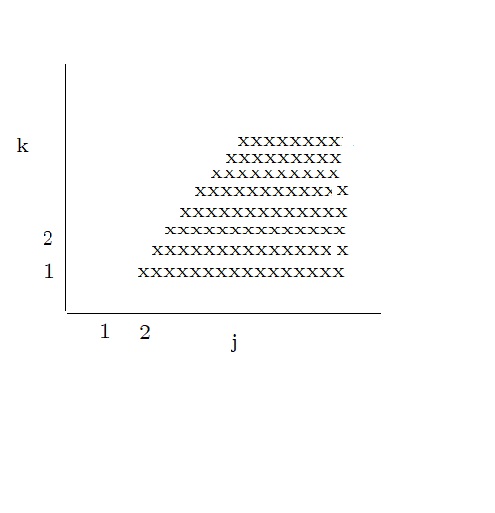
Figure 9: Allowed $k$ vs. $j$ region of summation

We get

$$\sum_{j=1}^{\infty}\sum_{k=1}^{\infty}(-1)^{\,j+k}\mathcal{V}_{1}^{\,}(\,j,k)=-\frac{Z}{2\pi^{3}}\frac{\lambda_{0}(r_{0})^{3/2}}{\sqrt{[\nu_{0}^{\left(1\right)}-1]\,}\omega_{0}\,r_{0}^{2}}\sum_{j=2}^{\infty}\sum_{k=1}^{j-1}\frac{(-1)^{j+k}\sin(2\pi j\,[\nu_{0}^{\left(1\right)}-1]\lambda_{0}(r_{0})-\pi/4)}{\,\,j^{1/2}\,[j^{2}-k^{2}]}.$$ (104)

Then the required expression for $V_{ne,\lambda,\nu}/Z$  becomes

$$-\frac{V_{ne,\lambda,\nu}}{Z}=\tfrac{4}{\pi^{3}}\tfrac{\sqrt{2}\lambda_{0}(r_{0})^{3/2}}{\sqrt{[\nu_{0}^{\left(1\right)}-1]\,}\omega_{0}\,r_{0}^{2}}\left\{\operatorname{Re}\mathcal{S}(x)+\operatorname{Im}\mathcal{S}(x)\right\},$$ (105)

with the complex quantity $x$ has been defined by

$$x=\exp\{2\pi i\,\,[\nu_{0}^{\left(1\right)}-1]\lambda_{0}(r_{0})\},$$

and

$$\mathcal{S}(x)=\sum_{j=2}^{\infty}\sum_{k=1}^{j-1}\frac{(-1)^{j+k}x^{\,j}}{\,\,j^{1/2}\,[j^{2}-k^{2}]}.$$

The double sum $\mathcal{S}(x)$ can be reduced to the terms (cf. Appendix B)

$$\mathcal{S}(x)=-\frac{1}{2}[\{1-\ln(2)\}x+\ln(2)Li_{3/2}(x)+Li_{5/2}(-x)]+\frac{1}{4}\sum_{j=2}^{\infty}\frac{x^{j}}{j^{3/2}}[\psi(j)-\psi(j+1/2)],$$ (106)

A closed-form expression for this expression is not known, however the infinite sum converges rapidly and may be safely truncated to contain eight terms to produce five figure accuracy.

Finally we have for $\overline{V}_{ne,\lambda}+\overline{V}_{ne,\lambda,\nu}$ the expression

$$-\frac{\overline{V}_{ne,\lambda}+\overline{V}_{ne,\lambda,\nu}}{Z} =\tfrac{\sqrt{2}}{\pi^{3}}\tfrac{\,\lambda_{0}(r_{0})^{3/2}}{\sqrt{[\nu_{0}^{\left(1\right)}-1]}\omega_{0}\,r_{0}^{2}}\left\{\operatorname{Re}[Li_{5/2}(-x)]+\operatorname{Im}[Li_{5/2}(-x)]\right\}$$ (107)

$$+\tfrac{4\sqrt{2}}{\pi^{3}}\tfrac{\lambda_{0}(r_{0})^{3/2}}{\sqrt{[\nu_{0}^{\left(1\right)}-1]\,}\omega_{0}\,r_{0}^{2}}\left\{\operatorname{Re}\mathcal{S}(x)+\operatorname{Im}\mathcal{S}(x)\right\},$$

with

$$\tfrac{\sqrt{2}}{\pi^{3}}\tfrac{\lambda_{0}(r_{0})^{3/2}}{\sqrt{[\nu_{0}^{\left(1\right)}-1]}\omega_{0}\,r_{0}^{2}}=0.033375Z^{1/2}.$$

1.13 The Schwinger-Englert Energy

As seen above the non-oscillating part of the chemical potential is zero, here we wish to evaluate the derivative of the SE energy in order to complete the calculation of the oscillating part of the chemical potential.

$$\mu_{osc}=\frac{dE(Z,Z)_{osc}}{dZ}-\frac{\overline{V}_{ne,osc}}{Z},$$

In the work by SE the $j,k$ plane is divided into regions within which the various contributions to the energy $E_{0}(Z,Z)$ have been computed.  They write the energy as

$$E_{osc}(Z,Z)=\sum_{k=1}^{\infty}E_{0,k}+\sum_{j=1}^{\infty}E_{j,0}+\sum_{j=1}^{\infty}\sum_{k=1}^{\infty}E_{j,k},$$ (108)

with

$$\sum_{k=1}^{\infty}E_{0,k} =E_{\,\mathit{l}TF}(Z),$$

$$\sum_{j=1}^{\infty}E_{j,0}+\sum_{j=1}^{\infty}\sum_{k=1}^{\infty}E_{j,k} =E_{\lambda-osc}(Z)+E_{\,\nu-osc}(Z)+E_{\nu,\lambda-osc}(Z).$$

In that work the energy associated with the $\nu$ oscillation was small and the $\lambda,\nu$ oscillations where found to be negligible compared to that of the $\lambda$ oscillations.  In the latter case the $E_{\nu,\lambda-osc}$ contribution is on the order of $0.000Z^{3/2}$ and has been dropped.  As a result we write

$$E(Z,Z)=E_{\,\mathit{l}TF}(Z)+E_{\,\lambda-osc}(Z)+E_{\,\nu-osc}(Z).$$ (109)

Schwinger and Englert have given $E_{\mathit{l}TF}\,(Z)$ as

$$E_{\,\mathit{l}\,TF}\,(Z)=\frac{\lambda_{0}}{r_{0}^{2}}[\frac{1}{2}\mathcal{K}_{1}C_{2}(\lambda_{0})-\lambda_{0}\nu_{0}^{{}^{(1)}}S_{1}(\lambda_{0})\,],$$ (110)

where the terms $C_{n}(\lambda_{0})$ and $S_{n}(\lambda_{0})$ are sums defined below and $\mathcal{K}_{1}$ is a constant i.e.

$$\mathcal{K}_{1}=-1+6\nu_{0}^{{}^{(1)}}-6(\nu_{0}^{(1)})^{3}+(\nu_{0}^{{}^{(1)}})^{5}=-5.709672$$

Noting the general relations for the sums

$$S_{n}(z) =\sum_{k=1}^{\infty}\frac{(-1)^{k}\sin(2\pi kz)}{(\pi k)^{2n+1}},$$

$$C_{n}(z) =\sum_{k=1}^{\infty}\frac{(-1)^{k}\cos(2\pi kz)}{(\pi k)^{2n}},$$

$$\frac{dS_{n}(z)}{dz} =2C_{n}(z),$$

$$\frac{dC_{n+1}(z)}{dz} =-2S_{n}(z),$$

and

$$\frac{d\lambda_{0}}{dZ} =\frac{1}{3}\left(\frac{\lambda_{0}}{Z}\right),$$

$$\frac{d}{dz}\left(\frac{\lambda_{0}^{3}}{\omega_{0}r_{0}^{3}}\right) =\frac{4}{3Z}\left(\frac{\lambda_{0}^{3}}{\omega_{0}r_{0}^{3}}\right),$$

$$\frac{d}{dz}\left(\frac{\lambda_{0}}{r_{0}^{2}}\right) =\frac{1}{Z}\left(\frac{\lambda_{0}}{r_{0}^{2}}\right),$$

we have

$$\frac{dE_{\,\mathit{l}\,TF}\,(Z)}{dZ}=\frac{2\lambda_{0}}{3Zr_{0}^{2}}[\frac{3}{2}\mathcal{K}_{1}C_{2}(\lambda_{0})+\lambda_{0}\{\nu_{0}^{{}^{(1)}}-\mathcal{K}_{1}\}S_{1}(\lambda_{0})+\lambda_{0}^{2}\,\nu_{0}^{{}^{(1)}}C_{1}(\lambda_{0})],$$ (111)

and

$$\frac{\lambda_{0}}{Zr_{0}^{2}}=0.26744$$

The terms in the derivative above are seen to be of order $Z^{0},Z^{1/3},Z^{2/3}$ respectively.

The SE energy of the $\lambda$ oscillations is given by

$$-(r_{0}/\lambda_{0})^{2}E_{\,\lambda-osc}(Z)=$$ (112)

$$\mathbf{S}_{1}^{\prime}(\lambda_{0})-\frac{1}{4}S_{1}(2\lambda_{0})+\mathcal{K}_{2}S_{0}(2\lambda_{0})-\lambda_{0}^{1/2}[\mathcal{K}_{3}\operatorname{Im}Li_{5/2}(-\exp(-4\pi i\lambda_{0}))]$$

$$+\frac{1}{Z^{1/3}}\left\{\begin{array}[c]{c}\mathcal{K}_{4}\left\{\mathbf{C}_{1}^{\prime}(\lambda_{0})+\frac{1}{8}\widetilde{C}_{2}(2\lambda_{0})\right\}-\mathcal{K}_{5}\mathbf{C}_{0}^{\prime}(\lambda_{0})+\mathcal{K}_{6}\widetilde{C}_{1}(2\lambda_{0})+\mathcal{K}_{7}\widetilde{C}_{0}(2\lambda_{0})\\ +\lambda_{0}^{1/2}[\mathcal{K}_{8}\operatorname{Re}Li_{7/2}(-\exp(-4\pi i\lambda_{0}))]+\lambda_{0}^{3/2}[\mathcal{K}_{9}\operatorname{Re}Li_{5/2}(-\exp(-4\pi i\lambda_{0}))]\end{array}\right\},$$

and

$$(\frac{\lambda_{0}}{r_{0}})^{2}=0.24818Z^{4/3},$$

where the terms $\mathbf{S}_{n}^{\prime}$ $\mathbf{C}_{n}^{\prime}$ $\widetilde{S}_{n}$ $\widetilde{C}_{n}$  are sums given below and the numerical constants $\mathcal{K}_{i}$ are

$$\mathcal{K}_{2} =[2-\nu_{0}^{{}^{(1)}}]/24\nu_{0}^{{}^{(1)}}=0.00134,$$

$$\mathcal{K}_{3} =\frac{\sqrt{3}}{\sqrt{\nu_{0}^{{}^{(1)}}[(\nu_{0}^{{}^{(1)}})^{2}-1][-15+23(\nu_{0}^{{}^{(1)}})^{2}-5(\nu_{0}^{{}^{(1)}})^{4}]}\pi^{2}}=0.04905,$$

$$\mathcal{K}_{4} =[3-4(\nu_{0}^{{}^{(1)}})^{2}]/(2\pi)^{4}=-0.00771,$$

$$\mathcal{K}_{5} =[1-\nu_{0}^{{}^{(1)}}]/4(\nu_{0}^{{}^{(1)}})^{3}=-0.03222,$$

$$\mathcal{K}_{6} =[34-48\nu_{0}^{{}^{(1)}}+31(\nu_{0}^{{}^{(1)}})^{2}]/576=0.09963,$$

$$\mathcal{K}_{7} =7[92-162\nu_{0}^{{}^{(1)}}+150(\nu_{0}^{{}^{(1)}})^{2}-76(\nu_{0}^{{}^{(1)}})^{3}+15(\nu_{0}^{{}^{(1)}})^{4}]/46080=-0.000026,$$

$$\mathcal{K}_{8} =\tfrac{[2(\nu_{0}^{{}^{(1)}})^{2}-1]}{(2\pi)^{3}}\sqrt{\tfrac{2}{\nu_{0}^{{}^{(1)}}-1}}=0.03832,$$

$$\mathcal{K}_{9} =\left(\tfrac{2}{\nu_{0}^{{}^{(1)}}-1}\right)^{3/2}[2-6\nu_{0}^{{}^{(1)}}-6(\nu_{0}^{{}^{(1)}})^{2}+12(\nu_{0}^{{}^{(1)}})^{3}-4(\nu_{0}^{{}^{(1)}})^{4}-2(\nu_{0}^{{}^{(1)}})^{5}-(\nu_{0}^{{}^{(1)}})^{6}]/(4\pi)^{4}$$

$$=-0.01359$$

The sums appearing above are given by [22]

$$\widetilde{S}_{0}(z) =\sum_{k=1}^{\infty}\frac{\sin(2\pi k\,z)}{(\pi k)}=-\left\langle z-1/2\right\rangle,$$

$$\widetilde{C}_{0}(z) =\sum_{k=1}^{\infty}\cos(2\pi k\,z)=-1/2,$$

$$\widetilde{S}_{1}(z) =\sum_{k=1}^{\infty}\frac{\sin(2\pi k\,z)}{(\pi k)^{3}}=\tfrac{2}{3}\left\langle z-1/2\right\rangle[\left\langle z-1/2\right\rangle^{2}-\tfrac{1}{4}],$$

$$\widetilde{C}_{1}(z) =\sum_{k=1}^{\infty}\frac{\cos(2\pi k\,z)}{(\pi k)^{2}}=\left\langle z-1/2\right\rangle^{2}-\tfrac{1}{12},$$

$$\widetilde{S}_{2}(z) =\sum_{k=1}^{\infty}\frac{\sin(2\pi k\,z)}{(\pi k)^{5}}=-\tfrac{1}{3}\left\langle z-1/2\right\rangle[\tfrac{2}{5}\left\langle z-1/2\right\rangle^{4}-\tfrac{1}{3}\left\langle z-1/2\right\rangle^{2}+\tfrac{7}{120}],$$

$$\widetilde{C}_{2}(z) =\sum_{k=1}^{\infty}\frac{\cos(2\pi k\,z)}{(\pi k)^{4}}=\tfrac{1}{90}-\tfrac{1}{3}[\left\langle z-1/2\right\rangle^{2}-\tfrac{1}{4}]^{2}.$$

and

$$\mathbf{S}_{0}^{\prime}(z) =\sum_{k=0}^{\infty}(-1)^{k}\sin(2\pi[2k+1]z)=0,$$

$$\mathbf{C}_{0}^{\prime}(z) =\sum_{k=0}^{\infty}\frac{(-1)^{k}\cos(2\pi[2k+1]z)}{[\pi(2k+1)]}=\tfrac{1}{4}(-1)^{\lfloor 2z+1/2\rfloor},$$

$$\mathbf{S}_{1}^{\prime}(z) =\sum_{k=0}^{\infty}\frac{(-1)^{k}\sin(2\pi[2k+1]z)}{[\pi(2k+1)]^{2}}=\tfrac{1}{2}[<z+\tfrac{1}{4}>^{2}-<z-\tfrac{1}{4}>^{2}],$$

$$\mathbf{C}_{1}^{\prime}(z) =\sum_{k=0}^{\infty}\frac{(-1)^{k}\cos(2\pi[2k+1]z)}{[\pi(2k+1)]^{3}},$$

$$=\tfrac{1}{3}[<z+\tfrac{1}{4}>\{\tfrac{1}{4}-<z+\tfrac{1}{4}>^{2}\}-<z-\tfrac{1}{4}>\{\tfrac{1}{4}-<z-\tfrac{1}{4}>^{2}\}].$$

The derivative of $E_{\,\lambda-osc}(Z)$ is given by

$$-3Z\,(r_{0}/\lambda_{0})^{2}\frac{dE_{\,\lambda-osc}(Z)}{dZ}=$$ (113)

$$4\mathbf{S}_{1}^{\prime}(\lambda_{0})-S_{1}(2\lambda_{0})+4\mathcal{K}_{2}S_{0}(2\lambda_{0})-\lambda_{0}^{1/2}[\tfrac{9}{2}\mathcal{K}_{3}\operatorname{Im}Li_{5/2}(-\exp(-4\pi i\lambda_{0}))]$$

$$+\lambda_{0}[2\mathbf{C}_{0}^{\prime}(\lambda_{0})-C_{1}(2\lambda_{0})]+\lambda_{0}^{3/2}[4\pi\,\mathcal{K}_{3}\operatorname{Re}Li_{3/2}(-\exp(-4\pi i\lambda_{0}))]$$

$$+\frac{1}{Z^{1/3}}\left\{\begin{array}[c]{c}\begin{array}[c]{c}3\mathcal{K}_{4}[\mathbf{C}_{1}^{\prime}(\lambda_{0})+\frac{1}{8}\widetilde{C}_{2}(2\lambda_{0})]-3\mathcal{K}_{5}\mathbf{C}_{0}^{\prime}(\lambda_{0})+3\mathcal{K}_{6}\widetilde{C}_{1}(2\lambda_{0})+3\mathcal{K}_{7}\widetilde{C}_{0}(2\lambda_{0})\\ +\,\lambda_{0}^{1/2}[\frac{7}{2}\mathcal{K}_{8}\operatorname{Re}Li_{7/2}(-\exp(-4\pi i\lambda_{0}))]\\ -2\lambda_{0}[\mathcal{K}_{4}\{\mathbf{S}_{1}^{\prime}(\lambda_{0})+\frac{1}{4}\widetilde{S}_{1}(2\lambda_{0})\}-\mathcal{K}_{5}\mathbf{S}_{0}^{\prime}(\lambda_{0})+2\mathcal{K}_{7}\widetilde{S}_{0}(2\lambda_{0})]\\ +\,\lambda_{0}^{3/2}[\frac{9}{2}\mathcal{K}_{9}\operatorname{Re}Li_{5/2}(-\exp(-4\pi i\lambda_{0}))+4\pi\,\mathcal{K}_{8}\operatorname{Im}Li_{5/2}(-\exp(-4\pi i\lambda_{0}))]\end{array}\\ +\lambda_{0}^{5/2}[4\pi\,\mathcal{K}_{9}\operatorname{Im}Li_{7/2}(-\exp(-4\pi i\lambda_{0}))].\end{array}\right\},$$

with

$$\frac{1}{Z\,}(\frac{\lambda_{0}}{r_{0}})^{2}=0.24818Z^{\,1/3}.$$

The $E_{\nu-osc}$ contribution to the energy is

$$E_{\nu-osc}=2(\lambda_{0}/r_{0})^{2}\mathcal{K}_{10}\,\widetilde{S}_{1}([1+\nu_{0}^{\prime}]\lambda_{0}/2),$$

where $\mathcal{K}_{10}$ is

$$\mathcal{K}_{10}=\frac{1}{[\left(\nu_{0}^{\prime}\right)^{2}-1][1+\nu_{0}^{\prime}-\left(\nu_{0}^{\prime}\right)^{2}-\left(\nu_{0}^{\prime}\right)^{3}+\left(\nu_{0}^{\prime}\right)^{4}]}=0.06046,$$

with $E_{\nu-osc}$ being on the order of $0.00Z^{4/3\text{ \ }}$which is small compared to the $\lambda$ oscillations. The derivative of $E_{\nu-osc}$ is

$$\frac{dE_{\nu-osc}}{dZ}=\frac{2}{3Z}(\frac{\lambda_{0}}{r_{0}})^{2}\mathcal{K}_{10}[4\widetilde{S}_{1}([1+\nu_{0}^{\prime}]\lambda_{0}/2)+[1+\nu_{0}^{\prime}]\lambda_{0}\widetilde{C}_{1}([1+\nu_{0}^{\prime}]\lambda_{0}/2)]$$

with $Z$ contributions to $dE_{\nu-osc}/dZ$ of order $Z^{2/3}$ and $\ Z^{1/3}$ and has been neglected.

1.14 Numerical Calculations

As a result of the analysis given above, the chemical potential is given by

$$\mu_{osc}=\frac{dE_{lTF}(Z)}{dZ}+\frac{dE_{\lambda-osc}(Z)}{dZ}-\frac{\overline{V}_{ne,lTF}}{Z}-\frac{\overline{V}_{ne,\lambda}+\overline{V}_{ne,\lambda,\nu}}{Z}.$$ (114)

The final calculation of the chemical potential can now proceed by combining the eqations above. The results of these calculations are shown in Figs. (10)

Figure 10 the oscillating part of the chemical potential vs. Z

The figure above shows the oscillating part of the chemical potential and therefore cannot be directly compared with the chemical potential in Fig. 1.  Furthermore the results are only valid for large Z. We see that in the semiclassical approximation to the potential energy that the fine scale oscillations disappointingly have been smoothed out.  In the case of very large Z relativistic effects are important but these have not been included in these calculations.

Appendix A

.14.1 Evaluation of the integrals $I_{1}(\nu,\lambda_{\varepsilon},r)$ and $I_{2}(\nu,\lambda_{\varepsilon},r)$
 

Here we give details of the calculation of $I_{1}$ and $I_{2}$.  In order for $I_{1}$ to be evaluated, i.e.

$$I_{1}(\nu,\lambda_{\varepsilon},r)=\int\sqrt{2r^{2}\{\varepsilon_{\lambda,\nu}-V\}-\lambda^{2}}d\nu,$$

a relationship must be established between $\varepsilon_{\lambda,\nu}$ and $\nu$ which will allow us to give an approximation for this integral.  We chose the Coulombic potential where this relationship is

$$\varepsilon_{\lambda,\nu}=-\frac{Z^{2}}{2\left(\lambda+\nu\right)^{2}}.$$

Then the integral $I_{1}(\nu)$ can be written as

$$I_{1}(\nu,\lambda_{\varepsilon},r)=-\frac{Zr}{2}\int\sqrt{\frac{\varepsilon_{\lambda,\nu}-V-\lambda^{2}/2r^{2}}{-\varepsilon_{\lambda,\nu}^{3}}}d\,\varepsilon_{\lambda,\nu},$$

which immediately produces

$$I_{1}(\nu,\lambda_{\varepsilon},r)=Zr\left[\sqrt{\frac{2r^{2}\left\{\varepsilon_{\lambda,\nu}-V\right\}-\lambda^{2}}{-2r^{2}\,\varepsilon_{\lambda,\nu}}}-\arctan\sqrt{\frac{2r^{2}\left\{\varepsilon_{\lambda,\nu}-V\right\}-\lambda^{2}}{-2r^{2}\,\varepsilon_{\lambda,\nu}}}\right].$$ (A1)

The value of that integral along the curves of degeneracy is then

$$I_{1}(\nu,\lambda_{\varepsilon},r)/Zr=\frac{\lambda_{\varepsilon}(r)}{Zr}\sqrt{\lambda_{\varepsilon}^{2}(r)-\lambda^{2}}-\arctan(\frac{\lambda_{\varepsilon}(r)}{Zr}\sqrt{\lambda_{\varepsilon}^{2}(r)-\lambda^{2}}),$$

where we have use the relations

$$\varepsilon_{\lambda,\nu(\lambda|\varepsilon)}=\varepsilon_{\lambda_{\varepsilon},0}=-Z^{2}/2\lambda_{\varepsilon}^{2},$$

and

$$\lambda_{\varepsilon}^{2}(r)=2r^{2}\left\{\varepsilon_{\lambda_{\varepsilon},\nu(\lambda|\varepsilon)}-V\right\},$$

or in terms of the angle $\theta$  (A1) becomes

$$\frac{I_{1}(\nu,\lambda_{\varepsilon},r)}{Zr}=\mathcal{K}_{\varepsilon}(r)\sin(\theta)-\arctan(\mathcal{K}_{\varepsilon}(r)\sin\theta),$$

where $\mathcal{K}_{\varepsilon}(r)=\lambda_{\varepsilon}^{2}/rZ$.  Since $\mathcal{K}_{\varepsilon}(r)\sin\theta$ is less than unity we have the final form of the integral

$$\frac{I_{1}(\nu,\lambda_{\varepsilon},r)}{Zr}=\tfrac{1}{3}[\mathcal{K}_{\varepsilon}(r)\sin(\theta)]^{3}-\tfrac{1}{5}[\mathcal{K}_{\varepsilon}(r)\sin(\theta)]^{5}+\cdots$$ (A2)

In a similar way, the integral for $I_{2}$ is

$$I_{2}(\nu,\lambda_{\varepsilon},r)=\sqrt{2}Z^{2}r\int\left[\sqrt{\tfrac{2r^{2}\left\{\varepsilon_{\lambda,\nu}-V\right\}-\lambda^{2}}{-2r^{2}\,\varepsilon_{\lambda,\nu}}}-\arctan\sqrt{\tfrac{2r^{2}\left\{\varepsilon_{\lambda,\nu}-V\right\}-\lambda^{2}}{-2r^{2}\,\varepsilon_{\lambda,\nu}}}\right]\frac{d\varepsilon_{\lambda,\nu}}{(-\varepsilon_{\lambda,\nu})^{3/2}},$$

which gives

$$I_{2}(\nu,\lambda,r)=$$

$$-\sqrt{2}Z^{2}r\left[\begin{array}[c]{c}-\tfrac{\sqrt{2r^{2}\left\{\varepsilon_{\lambda,\nu}-V\right\}-\lambda^{2}}}{\sqrt{2}r\varepsilon_{\lambda,\nu}}+\frac{2}{\sqrt{-\varepsilon_{\lambda,\nu}}}\arctan\sqrt{\frac{2r^{2}\left\{\varepsilon_{\lambda,\nu}-V\right\}-\lambda^{2}}{-2r^{2}\,\varepsilon_{\lambda,\nu}}}\\ -\,\frac{\sqrt{2}r}{\sqrt{2r^{2\{}\varepsilon_{\lambda,\nu}-V\}-\lambda^{2}-2r^{2}\varepsilon_{\lambda,\nu}}}\ln(\sqrt{\frac{2r^{2}\left\{\varepsilon_{\lambda,\nu}-V\right\}-\lambda^{2}}{-2r^{2}\,\varepsilon_{\lambda,\nu}}}-\sqrt{\tfrac{2r^{2}\{\varepsilon_{\lambda,\nu}-V\}-\lambda^{2}-2r^{2}\varepsilon_{\lambda,\nu}}{-2r^{2}\varepsilon_{\lambda,\nu}}})\end{array}\right].$$

Then

$$I_{2}(\nu,\lambda_{\varepsilon},r) =2\lambda_{\varepsilon}^{2}\sqrt{\lambda_{\varepsilon}^{2}-\lambda^{2}}-4Zr\lambda_{\varepsilon}\arctan(\frac{\lambda_{\varepsilon}\sqrt{\lambda_{\varepsilon}^{2}-\lambda^{2}}}{rZ})$$

$$+\frac{2r^{2}Z^{2}\lambda_{\varepsilon}}{\sqrt{r^{2}Z^{2}+\lambda_{\varepsilon}^{2}(\lambda_{\varepsilon}^{2}-\lambda^{2})}}\ln(\frac{\lambda_{\varepsilon}\sqrt{\lambda_{\varepsilon}^{2}-\lambda^{2}}}{rZ}-\frac{\sqrt{\lambda_{\varepsilon}^{2}(\lambda_{\varepsilon}^{2}-\lambda^{2})+r^{2}Z^{2}}}{rZ})$$

or with $\lambda=\lambda_{\varepsilon}\cos\theta$ we have

$$I_{2}(\nu,\lambda_{\varepsilon},r)/2rZ\lambda_{\varepsilon} =\frac{\lambda_{\varepsilon}^{2}}{rZ}\sin\theta-2\arctan(\frac{\lambda_{\varepsilon}^{2}}{rZ}\sin\theta)$$

$$+\frac{1}{\sqrt{1+[\frac{\lambda_{\varepsilon}^{2}}{rZ}\sin\theta]^{2}}}\ln(\frac{\lambda_{\varepsilon}^{2}}{rZ}\sin\theta-\sqrt{[\frac{\lambda_{\varepsilon}^{2}}{rZ}\sin\theta]^{2}+1]}\,),$$

In the more compact form $I_{2}(\nu,\lambda_{\varepsilon},r)$ becomes

$$\frac{I_{2}(\nu,\lambda_{\varepsilon},r)}{2rZ\lambda_{\varepsilon}}=\mathcal{K}_{\varepsilon}(r)\sin\theta-2\arctan(\mathcal{K}_{\varepsilon}(r)\sin\theta)+\frac{\arcsin h\,(\mathcal{K}_{\varepsilon}(r)\sin\theta)}{\sqrt{1+[\mathcal{K}_{\varepsilon}(r_{\varepsilon})\sin\theta]^{2}}}.$$ (A3)

For small argument $\mathcal{K}_{\varepsilon}(r)\sin\theta$ we have

$$\frac{I_{2}(\nu,\lambda_{\varepsilon},r)}{2rZ\lambda_{\varepsilon}}=\tfrac{2}{15}\left[\mathcal{K}_{\varepsilon}(r)\sin\theta\right]^{5}-\tfrac{6}{35}\left[\mathcal{K}_{\varepsilon}(r)\sin\theta\right]^{7}+\cdots.$$ (A4)

Appendix B

The double sum

$$\mathcal{S}(x)=\sum_{j=2}^{\infty}\sum_{k=1}^{j-1}\frac{(-1)^{j+k}x^{j}}{\,\,j^{1/2}\,[j^{2}-k^{2}]},$$

with $x=\exp(i\theta)$ and $\theta=2\pi[\,[\nu_{0}^{\left(1\right)}-1]\lambda_{0}(r_{0})$ $]$ can be simplified as follows.  The sum over $k$ can be written as

$$\sum_{k=1}^{j-1}\frac{(-1)^{k}}{\,\,[j^{2}-k^{2}]}=-\frac{1}{2j^{2}}-\frac{(-1)^{j}}{j}\{\frac{1}{2}\ln(2)+\frac{1}{4}\psi(j+1/2)-\frac{1}{4}\psi(j)\},$$

where $\psi$ is the digamma function.  Then $\mathcal{S}(x)$is given by

$$\mathcal{S}(x) =-\frac{1}{2}[\{1-\ln(2)\}x+\ln(2)Li_{3/2}(x)+Li_{5/2}(-x)]+\frac{1}{4}\sum_{j=2}^{\infty}\frac{x^{j}}{j^{3/2}}[\psi(j)-\psi(j+1/2)],$$

$$=-\frac{1}{2}[\{1-\ln(2)\}x+\ln(2)Li_{3/2}(x)-Li_{5/2}(x)+\frac{1}{2^{3/2}}Li_{5/2}(x^{2})]$$

$$+\frac{1}{4}\sum_{j=2}^{\infty}\frac{x^{j}}{j^{3/2}}[\psi(j)-\psi(j+1/2)],$$

The remaining sum in  the equation above is rapidly convergent, eight terms being sufficient for six figure accuracy.

Appendix C

.15 The Primitive Integrals $C_{ss},$ $S_{ss},$ $C_{cs},$ $S_{sc}$

The key primitive integrals $C_{ss},S_{ss},C_{cs},S_{sc}$ which appear in the text above and where $z$ and $\varrho$ are $<0$ i.e.

$$\mathcal{C}_{cc}\mathcal{(}\kappa,z,\varrho) =\int_{0}^{\pi/2}\sin^{2\kappa+2\,}\theta\cos\theta\cos(z\cos\theta)\cos(\varrho\cos^{2}\theta)d\theta,$$ (C1)

$$\mathcal{S}_{ss}\mathcal{(}\kappa,z,\varrho) =\int_{0}^{\pi/2}\sin^{2\kappa+2\,}\theta\cos\theta\sin(z\cos\theta)\sin(\varrho\cos^{2}\theta)d\theta,$$

$$\mathcal{C}_{cs}\mathcal{(}\kappa,z,\varrho) =\int_{0}^{\pi/2}\sin^{2\kappa+2\,}\theta\cos\theta\cos(z\cos\theta)\sin(\varrho\cos^{2}\theta)d\theta,$$

$$\mathcal{S}_{sc}\mathcal{(}\kappa,z,\varrho) =\int_{0}^{\pi/2}\sin^{2\kappa+2\,}\theta\cos\theta\sin(z\cos\theta)\cos(\varrho\cos^{2}\theta)d\theta.$$

can be expressed in terms of the integrals$\ \mathcal{J}(\kappa,\,j,a,z),$ and $\mathcal{H}(\kappa,\,j,a,z)$ which have closed forms and are defined as

$$\mathcal{J}(\kappa,\,j,a,z)=\int_{0}^{\pi/2}\sin^{2\kappa+2\,}\theta\,\cos^{4\,j+2\,a+1}\theta\,\sin(z\cos\theta)\,d\theta,$$

$$\mathcal{H}(\kappa,\,j,a,z)=\int_{0}^{\pi/2}\sin^{2\kappa+2\,}\theta\,\cos^{4\,j+2\,a+1}\theta\,\cos(z\cos\theta)\,d\theta.$$

The latter integrals are given by Maple as

$$\mathcal{J}(\kappa,\,j,a,z)=\tfrac{1}{2}z\,B(2j+a+3/2,\kappa+3/2)\,_{1}F_{2}\tbinom{2\,j+a+3/2\,;\,-z^{2}/4}{3/2\,,\,\kappa+2\,j+a+3},$$

$$\mathcal{H}(\kappa,\,j,a,z)=\tfrac{1}{2}B(2j+a+1,\kappa+3/2)\,_{1}F_{2}\tbinom{2\,j+a+1\,;\,-z^{2}/4}{1/2\,,\,\kappa+2\,j+a+5/2},$$

where $B(\alpha,\beta)$ is the Beta function and ${}_{1}F_{2}\tbinom{a_{1\,};\,z}{b_{1}\,,\,b_{2}}$ is a generalized hypergeometic function.  As will be seen below, these integrals are also expressible in terms of quantities which involve only products of the Bessel functions $J_{0}(z)$, and $J_{1}(z)$ or the Struve functions $\mathbf{H}_{0}(z),$ $\mathbf{H}_{1}(z)$, and polynomials with arguments $1/z.$ That is to say

$$\mathcal{J\,}(\kappa,\,j,a,z)$$ (C2)

$$=(-1)^{a+1}\tfrac{\pi}{2}[J_{0}(z)\,{\Large\wp}(\kappa,{\small 4j+2a+1},z)+J_{1}(z)\,\mathcal{Q}(\kappa,{\small 4j+2a+1},z)],$$

$$\mathcal{H}(\kappa,\,j,a,z)$$ (C3)

$$=({\small-1)}^{a}\tfrac{\pi}{2}[\mathbf{H}_{0}{\small(z)}{\Large\wp}({\small\kappa,4j+2a+1,z}){\small+}\mathbf{H}_{1}{\small(z)\,}\mathcal{Q}({\small\kappa},{\small 4j+2a+1,z}){\small+}\tfrac{2}{\pi}\mathcal{R(}{\small\kappa,4j+2a+1,z})],$$

where the quantities $${\Large\wp,}\mathcal{Q} \mathcal{R}$$, are related to the Lommel polynomials.  In the latter forms the oscillatory behavior of these integrals and those of the key integrals mentioned above is made manifest.

.15.1 Proof of The $\mathcal{J\,}(\kappa,\,j,a,z)$ and $\mathcal{H}(\kappa,\,j,a,z)$ expressions

Using the integral representations for Bessel functions of the first kind $J_{\nu}(z)$ and the Struve functions $\mathbf{H}_{\nu}(z)$ [25] i.e.

$$\tfrac{\sqrt{\pi}\Gamma(\nu+1/2)}{2}\frac{J_{\nu}(z)}{\left(z/2\right)^{\nu}}=\int_{0}^{\pi/2}\sin^{2\nu}\theta\cos(z\cos\theta)\,d\theta,$$

$$\tfrac{\sqrt{\pi}\Gamma(\nu+1/2)}{2}\frac{\mathbf{H}_{\nu}(z)}{(z/2)^{\nu}}=\int_{0}^{\pi/2}\sin^{2\nu}\theta\sin(z\cos\theta)\,d\theta,$$

and differentiating these expressions with respect to $z,$ $4j+2a+1$ times gives

$$\mathcal{J}(\kappa,\,j,a,z)=(-1)^{a+1}\tfrac{\pi}{2}{\small(}2\kappa+1{\small)!!}\frac{d^{\,\,4\,j+2\,a+1}[J_{\kappa+1}(z)/z^{\kappa+1}]}{d\,z^{\,4\,j+2\,a+1}},$$ (C4)

$$\mathcal{H}(\kappa,\,j,a,z)=(-1)^{a}\tfrac{\pi}{2}{\small(}2\kappa+1{\small)!!}\frac{d^{\,\,4\,j+2\,a+1}[\mathbf{H}_{\kappa+1}(z)/z^{\kappa+1}]}{d\,z^{\,4\,j+2\,a+1}},$$ (C5)

where $(2\kappa+1)!!$ is the double factorial function i.e.

$$(2\kappa+1)!!=\prod_{i=1}^{\kappa}(2i+1)=\frac{2^{\kappa+1}}{\sqrt{\pi}}\Gamma(\kappa+3/2).$$

We have by direct observation [26]that for $\nu\geq 0,$

$$(2\kappa+1)!!\frac{d^{\,\nu}}{d\,z^{\,\nu}}[\frac{J_{\kappa+1}(z)}{z^{\kappa+1}}] ={\Large\wp}(\kappa,\nu,z)\,J_{0}(z)\,\,+\mathcal{Q}(\kappa,\nu,z)\,J_{1}(z)\,,$$ (C6)

$$(2\kappa+1)!!\frac{d^{\,\nu}}{d\,z^{\,\nu}}[\frac{\mathbf{H}_{\kappa+1}(z)}{z^{\kappa+1}}] ={\Large\wp}(\kappa,\nu,z)\,\mathbf{H}_{0}(z)\,\,+\mathcal{Q}(\kappa,\nu,z)\,\mathbf{H}_{1}(z)+\tfrac{2}{\pi}\,\mathcal{R(}\kappa,\nu,z),$$ (C7)

Using (C4) and (C5) together with (C6) and (C7) we get (C2) and (C3).

.16 Properties of the Polynomials ${\LARGE\wp}(\kappa,\nu,z)$, $\mathcal{Q}(\kappa,\nu,z)$, and $\mathcal{R(}\kappa,\nu,z)$

The polynomials ${\Large\wp}(\kappa,\nu,z)$, $\mathcal{Q}(\kappa,\nu,z),$ and $\mathcal{R(}\kappa,\nu,z)$ are interrelated by differential recurrence relations (which follow from the expressions for $\frac{d^{\,\nu+1}}{d\,z^{\,\nu+1}}[\frac{J_{\kappa+1}(z)}{z^{\kappa+1}}]$ and $\frac{d^{\,\nu+1}}{d\,z^{\,\nu+1}}[\frac{\mathbf{H}_{\kappa+1}(z)}{z^{\kappa+1}}]$ and the linear independence of the Bessel $J_{0}$, $J_{1}$ and Struve functions $\mathbf{H}_{0}$, $\mathbf{H}_{1}$), we have

$${\Large\wp}(\kappa,\nu+1,z) =\frac{d{\Large\wp}(\kappa,\nu,z)}{dz}+\mathcal{Q}(\kappa,\nu,z),$$ (C8)

$$\mathcal{Q}(\kappa,\nu+1,z) =\frac{d\mathcal{Q}(\kappa,\nu,z)}{dz}-{\Large\wp}(\kappa,\nu,z)-\frac{\mathcal{Q}(\kappa,\nu,z)}{z},$$

$$\mathcal{R(}\kappa,\nu+1,z) =\frac{d\,\mathcal{R(}\kappa,\nu,z)}{dz}+{\Large\wp}(\kappa,\nu,z).$$

with

$${\Large\wp}(0,1,z) =1/z,$$

$$\mathcal{Q}(0,1,z) =-2/z^{2},$$

$$\mathcal{R(}0,1,z) =0.$$

In addition it follows from the differential equations defining $J_{\kappa+1}(z)$ and $\mathbf{H}_{\kappa+1}(z)$ that the functions $J_{\kappa+1}(z)/z^{\kappa+1}$ and $\mathbf{H}_{\kappa+1}(z)/z^{\kappa+1}$ satisfy the differential equations

$$z\frac{d^{\,2}\left[J_{\kappa+1}(z)/z^{\kappa+1}\right]}{d\,z^{2}}+(2\kappa+3)\frac{d\,\left[J_{\kappa+1}(z)/z^{\kappa+1}\right]}{d\,z}+z[J_{\kappa+1}(z)/z^{\kappa+1}]=0,$$

$$z\frac{d^{\,2}\left[\mathbf{H}_{\kappa+1}(z)/z^{\kappa+1}\right]}{d\,z^{2}}+(2\kappa+3)\frac{d\,\left[\mathbf{H}_{\kappa+1}(z)/z^{\kappa+1}\right]}{d\,z}+z[\mathbf{H}_{\kappa+1}(z)/z^{\kappa+1}]=\frac{2}{\pi(2\kappa+1)!!\,}.$$

Repeated differentiation of these relations gives for $\nu\geq 3,$

$$z\frac{d^{\,\nu}\Im(\kappa,z)}{d\,z^{\nu}}+(2\kappa+\nu+1)\frac{d^{\,\nu-1}\Im(\kappa,z)}{d\,z^{\nu-1}}+z\frac{d^{\,\nu-2}\Im(\kappa,z)}{d\,z^{\nu-2}}+(\nu-2)\frac{d^{\,\nu-3}\Im(\kappa,z)}{d\,z^{\nu-3}}=0,$$

where $\Im(\kappa,z)$ is either $J_{\kappa+1}(z)/z^{\kappa+1}$ or $\mathbf{H}_{\kappa+1}(z)/z^{\kappa+1}.$ Using (C2) and (C3) it follows that the coefficients of the functions $J_{0}(z)$, $\ J_{1}(z),$ $\mathbf{H}_{0}(z),$ and $\mathbf{H}_{1}(z)$ in the resulting relations vanish and we get the pseudo 4th-order recurrence relations

$$z\,F(\kappa,\nu,z)+(2\kappa+\nu+1)F(\kappa,\nu-1,z)+z\,F(\kappa,\nu-2,z)+(\nu-2)F(\kappa,\nu-3,z)=0,\hskip 18.06749pt\nu\geq 3$$

where $F(\kappa,\nu,z)$ stands for any of the polynomials ${\Large\wp}(\kappa,\nu,z),$ $\mathcal{Q}(\kappa,\nu,z),$ $\mathcal{R(}\kappa,\nu,z)$.  In the special case where $\nu<3$ the $\mathcal{R(}\kappa,\nu,z)$ polynomials are interrelated by

$$z\,\mathcal{R}(\kappa,2,z)+(2\kappa+3)\mathcal{R}(\kappa,1,z)+z\,\mathcal{R}(\kappa,0,z)=1.$$

We also note that since

$$(2\kappa+3)!!\frac{d^{\,\nu}}{d\,z^{\,\nu}}\left[\frac{J_{\kappa+2}(z)}{z^{\kappa+2}}\right]=(2\kappa+1)!!\left\{\frac{d^{\,\nu}}{d\,z^{\,\nu}}\left[\frac{J_{\kappa+1}(z)}{z^{\kappa+1}}\right]+\frac{d^{\,\nu+2}}{d\,z^{\,\nu+2}}\left[\frac{J_{\kappa+1}(z)}{z^{\kappa+1}}\right]\right\},$$

(as well as the corresponding relation for the $\mathbf{H}_{\kappa+1}(z)/z^{\kappa+1}$) it follows from the definition of the polynomial ${\Large\wp}(\kappa,\nu,z),$ $\mathcal{Q}(\kappa,\nu,z),$ $\mathcal{R(}\kappa,\nu,z)$, that they also satisfy partial difference equations in $\kappa$ and $\nu,$ we have

$$F(\kappa+1,\nu,z)=F(\kappa,\nu,z)+F(\kappa,\nu+2,z).$$

In summary, we will see that all of the integrals occurring above in the body of the text can be expressed in terms of the Bessel and Struve functions of orders zero and one together with the polynomials ${\Large\wp}(\kappa,\nu,z),$ $\mathcal{Q}(\kappa,\nu,z),$ $\mathcal{R(}\kappa,\nu,z)$ or the Lommel polynomials $R_{m,\nu}(z)$.

Below, the polynomials${\Large\wp,}$ $\mathcal{Q},$ and $\mathcal{R}$ and their relation to the Lommel polynomials [27]$\ R_{m,\nu}(z)$ is examined.

.17 ${\Large\wp}(\kappa,\nu,z),$ $\mathcal{Q}(\kappa,\nu,z),$ and $\mathcal{R(}\kappa,\nu,z)$ and the Lommel polynomials

As will be seen below, the polynomials ${\Large\wp}(\kappa,\nu,z)$, $\mathcal{Q}(\kappa,\nu,z),$ and $\mathcal{R(}\kappa,\nu,z)$ can be expressed explicitly as sums of the Lommel polynomials $R_{m,\nu}(z)$ the latter being given by

$$R_{m,\nu}(z)=\sum_{n=0}^{\lceil\frac{m}{2}\rceil}\frac{(-1)^{n}(m-n)!\Gamma(\nu+m-n)}{n!(m-2n)!\Gamma(\nu+n)}(2/z)^{m-2n}.$$ (C9)

Using (C9), we see that the leading terms for the Lommel polynomials are

$$R_{2\kappa,\ \mu}(z) \thicksim(-1)^{\kappa}[1-2\kappa(\kappa+1)(\kappa+\mu-1)(\kappa+\mu)/z^{2}]+\cdots,$$

$$R_{2\kappa+1,\ \mu}(z) \thicksim(-1)^{\kappa}2(\kappa+1)(\kappa+\mu)/z+\cdots,$$

expressions which will be useful in the sequel in obtaining the leading terms of the ${\Large\wp}(\kappa,\nu,z)$, $\mathcal{Q}(\kappa,\nu,z),$ and $\mathcal{R(}\kappa,\nu,z)$ polynomials.

It is important to note that the $R_{m,\nu}(z)$ polynomials can also be generated by the Bessel function relations [30] first obtained by Lommel i.e.

$$J_{\mu+m}(z)=J_{\mu}(z)\ R_{m,\ \mu}(z)-J_{\mu-1}(z)\ R_{m-1,\ \mu+1}(z).$$ (C10)

The corresponding relations involving the Struve functions while being more complicated are given by [28]

$$\mathbf{H}_{\mu+m}(z) =\mathbf{H}_{\mu}(z)\ R_{m,\ \mu}(z)-\mathbf{H}_{\mu-1}(z)\ R_{m-1,\ \mu+1}(z)$$ (C11)

$$+\frac{1}{\sqrt{\pi}}\left(\frac{z}{2}\right)^{\mu+m-1}\sum_{j=0}^{m-1}\frac{R_{j,\ \mu+m-j}(z)}{\Gamma(\mu+m+1/2-j)}\left(\frac{2}{z}\right)^{j}.$$

Generalizing differential expressions due to Brychkov [29] we have the relations

$$\frac{d^{\,\nu}\,\left[J_{\kappa+1}(z)/z^{\kappa+1}\right]}{d\,z^{\,\nu}}=\frac{(-1)^{\nu}\nu!}{z^{\kappa+1}}\sum_{i=0}^{\lfloor\frac{\nu}{2}\rfloor}\frac{(-1)^{i}J_{\kappa+1+\nu-i}(z)}{i!(\nu-2i)!(2z)^{i}}$$ (C12)

$$\frac{d^{\,\nu}\,\left[\mathbf{H}_{\kappa+1}(z)/z^{\kappa+1}\right]}{d\,z^{\,\nu}} =\frac{(-1)^{\nu}\nu!}{z^{\kappa+1}}\sum_{i=0}^{\lfloor\frac{\nu}{2}\rfloor}\frac{(-1)^{i}\mathbf{H}_{\kappa+1+\nu-i}(z)}{i!(\nu-2i)!(2z)^{i}}$$

$$+\frac{(-1)^{\nu+1}\nu!(z/2)^{\nu-1}}{\pi\ 2^{\kappa+1}}\sum_{i=0}^{\lfloor\frac{\nu}{2}\rfloor}\frac{(-1)^{i}}{i!(\nu-2i)!\ (z)^{2i}}\sum_{j=0}^{\nu-1-i}\frac{\Gamma(j+1/2)}{\Gamma(\kappa+3/2+\nu-j-i)}(\frac{2}{z})^{2j}.$$ (C13)

Using  Eq. (C10) with $\mu=1$ and $\kappa$ replaced by $\kappa+\nu-i$ in Eqs. (C12) and (C13) we get using Eqs. (C6) and (C7) the desired expressions for the ${\Large\wp}(\kappa,\nu,z)$, $\mathcal{Q}(\kappa,\nu,z),$ and $\mathcal{R(}\kappa,\nu,z)$ polynomials. (computed in Lommelmarch4.mw)

$${\Large\wp}(\kappa,\nu,z)\, =\frac{(-1)^{\nu+1}\nu!(2\kappa+1)!!}{z^{\kappa+1}}\sum_{i=0}^{\lfloor\frac{\nu}{2}\rfloor}\frac{(-1)^{i}R_{\kappa+\nu-1-i},_{2}(z)}{i!(\nu-2i)!(2z)^{i}},$$

$$\mathcal{Q}(\kappa,\nu,z) =\frac{(-1)^{\nu}\nu!(2\kappa+1)!!}{z^{\kappa+1}}\sum_{i=0}^{\lfloor\frac{\nu}{2}\rfloor}\frac{(-1)^{i}R_{\kappa+\nu-i},_{1}(z)}{i!(\nu-2i)!(2z)^{i}},$$

$$\mathcal{R(}\kappa,\nu,z) =\frac{(-z/2)^{\nu-1}\,\nu!(2\kappa+1)!!}{2^{\kappa+2}}[\sum_{m=0}^{\lfloor\frac{\nu}{2}\rfloor}\frac{c(\nu,m,m)\,}{\Gamma(\kappa+\nu+3/2-m)}(\frac{2}{z})^{2m}$$

$$+\sum_{m=\,\lfloor\frac{\nu}{2}\rfloor+1}^{\nu-1}\frac{c(\nu,m,\lfloor\frac{\nu}{2}\rfloor)\,}{\Gamma(\kappa+\nu+3/2-m)}(\frac{2}{z})^{2m}$$

$$-\sum_{i=0}^{\lfloor\frac{\nu}{2}\rfloor}\frac{(-1/z^{2})^{i}}{i!(\nu-2i)!}\sum_{j=0}^{\kappa+\nu-1-i}\frac{\sqrt{\pi}R_{j,\,\kappa+\nu+1-i-j}(z)\,}{\Gamma(\kappa+\nu+3/2-i-j)}(\frac{2}{z})^{\,j}],$$

where the coefficients $c(\nu,m,N)$ are given by

$$c(\nu,m,N)=\sum_{j=0}^{N}\frac{(-1/4)^{\,j}\Gamma(m+1/2-j)}{j!(\nu-2j)!}.$$

In the case of ${\Large\wp}(\kappa,\nu,z)$, and $\mathcal{Q}(\kappa,\nu,z)$ it is interesting to note that only higher powers of $1/z$ occur. The leading terms of these polynomials are then given by

$${\Large\wp}(2\kappa,2\mu+1,z) \thicksim(-1)^{\kappa+\mu}(4\kappa+1)!!/z^{2\kappa+1},$$

$${\Large\wp}(2\kappa+1,2\mu+1,z) \thicksim(-1)^{\kappa+\mu}(4\kappa+3)!!\{2\kappa^{2}+2\kappa[2\mu+3]+7\mu+4\}/z^{2\kappa+3},$$

$${\Large\wp}(2\kappa,2\mu,z) \thicksim(-1)^{\kappa+\mu}(4\kappa+1)!!\{2\kappa^{2}+2\kappa[2\mu+1]+3\mu\}/z^{2\kappa+2},$$

$${\Large\wp}(2\kappa+1,2\mu,z) \thicksim(-1)^{\kappa+\mu+1}(4\kappa+3)!!/z^{2\kappa+2},$$

and

$$\mathcal{Q}(2\kappa,2\mu+1,z) \thicksim(-1)^{\kappa+\mu+1}(4\kappa+1)!!\{2\kappa^{2}+4\kappa[\mu+1]+3\mu+2\}/z^{2\kappa+2},$$

$$\mathcal{Q}(2\kappa+1,2\mu+1,z) \thicksim(-1)^{\kappa+\mu}(4\kappa+3)!!/z^{2\kappa+2},$$

$$\mathcal{Q}(2\kappa,2\mu,z) \thicksim(-1)^{\kappa+\mu}(4\kappa+1)!!/z^{2\kappa+1},$$

$$\mathcal{Q}(2\kappa+1,2\mu,z) \thicksim(-1)^{\kappa+\mu}(4\kappa+3)!!\{2\kappa^{2}+4\kappa[\mu+1]+5\mu+2\}/z^{2\kappa+3}.$$

In the case of the polynomials $\mathcal{R(}\kappa,\mu,z)$ the leading terms are more difficult to obtain.  Using the differential difference equations for the ${\Large\wp}(\kappa,\nu,z)$, $\mathcal{Q}(\kappa,\nu,z),$ and $\mathcal{R(}\kappa,\nu,z)$ polynomials we get

$$\mathcal{R(}\kappa,\nu,z) =\frac{d^{\,\nu-1}\mathcal{R(}\kappa,1,z)}{d\,z^{\,\nu-1}}+\sum_{j=1}^{\nu-1}\frac{d^{\,\nu-1-j}{\Large\wp}\mathcal{(}\kappa,j,z)}{d\,z^{\,\nu-1-j}},$$

$$\mathcal{R(}\kappa,\nu,z) \thicksim(-1)^{\nu}\frac{\nu!}{z^{\nu+1}}+{\Large\wp}\mathcal{(}\kappa,\nu-1,z)+\frac{d^{\,}{\Large\wp}\mathcal{(}\kappa,\nu-2,z)}{d\,z^{\,}}+\cdots,\nu>2,$$

$$\mathcal{R(}\kappa,\nu,z) \thicksim(-1)^{\nu}\frac{\nu!}{z^{\nu+1}}+2{\Large\wp}\mathcal{(}\kappa,\nu-1,z)-\mathcal{Q(}\kappa,\nu-2,z).$$

Using the leading term expressions for the ${\Large\wp}(\kappa,\nu,z)$, and $\mathcal{Q}(\kappa,\nu,z)$ polynomials we get

$$\mathcal{R(}2\kappa+1,2\mu,z)\thicksim\left\{\begin{tabular}[c]{c}$(2\mu)!/z^{2\mu+1},\hskip 18.06749pt\mu\leq\kappa,$\\ $(-1)^{\kappa+\mu+1}(4\kappa+3)!!\{2\kappa^{2}+4\kappa(\mu+1)+5\mu+1\}/z^{2\kappa+3},\hskip 18.06749pt\mu>\kappa,$\end{tabular}\right.,$$

$$\mathcal{R(}2\kappa+1,2\mu+1,z)\thicksim\left\{\begin{tabular}[c]{c}$-(2\mu+1)!/z^{2\mu+2},\hskip 18.06749pt\mu<\kappa,$\\ $-[(4\kappa+3)!!+(2\kappa+1)!]/z^{2\kappa+2},\hskip 18.06749pt\mu=\kappa,$\\ $(-1)^{\kappa+\mu+1}(4\kappa+3)!!/z^{2\kappa+2},\hskip 18.06749pt\mu>\kappa,$\end{tabular}\right.,$$

$$\mathcal{R(}2\kappa,2\mu+1,z)\thicksim\left\{\begin{tabular}[c]{c}$-(2\mu+1)!/z^{2\mu+2},\hskip 18.06749pt\mu<\kappa,$\\ $[(4\kappa+1)!!\{6\kappa^{2}+7\kappa+1\}-(2\kappa+1)!]/z^{2\kappa+2},\hskip 18.06749pt\mu=\kappa,$\\ $(-1)^{\kappa+\mu}(4\kappa+1)!!\{2\kappa^{2}+4\kappa(\mu+1)+3\mu+1\}/z^{2\kappa+2},\hskip 18.06749pt\mu>\kappa,$\end{tabular}\right.,$$

$$\mathcal{R(}2\kappa,2\mu,z)\thicksim\left\{\begin{tabular}[c]{c}$(2\mu)!/z^{2\mu+1},\hskip 18.06749pt\mu<\kappa,$\\ $-[(4\kappa+1)!!-(2\kappa)!]/z^{2\kappa+1},\hskip 18.06749pt\mu=\kappa,$\\ $(-1)^{\kappa+\mu+1}(4\kappa+1)!!/z^{2\kappa+1},\hskip 18.06749pt\mu>\kappa,$\end{tabular}\right..$$

.17.1 The Integrals $\ \mathcal{C}_{cc},\mathcal{S}_{ss},\mathcal{C}_{cs},\mathcal{S}_{sc}$ and $T_{cc},T_{ss},T_{sc},T_{cs}$

Recalling the integrals $\mathcal{C}_{cc},\mathcal{S}_{ss},\mathcal{C}_{cs},\mathcal{S}_{sc}$ defined above .i.e.

$$\mathcal{C}_{cc}\mathcal{(}\kappa,z,\varrho) =\int_{0}^{\pi/2}\sin^{2\kappa+2\,}\theta\cos\theta\cos(z\cos\theta)\cos(\varrho\cos^{2}\theta)d\theta,$$ (C14)

$$\mathcal{S}_{ss}\mathcal{(}\kappa,z,\varrho) =\int_{0}^{\pi/2}\sin^{2\kappa+2\,}\theta\cos\theta\sin(z\cos\theta)\sin(\varrho\cos^{2}\theta)d\theta,$$

$$\mathcal{C}_{cs}\mathcal{(}\kappa,z,\varrho) =\int_{0}^{\pi/2}\sin^{2\kappa+2\,}\theta\cos\theta\cos(z\cos\theta)\sin(\varrho\cos^{2}\theta)d\theta,$$

$$\mathcal{S}_{sc}\mathcal{(}\kappa,z,\varrho) =\int_{0}^{\pi/2}\sin^{2\kappa+2\,}\theta\cos\theta\sin(z\cos\theta)\cos(\varrho\cos^{2}\theta)d\theta,$$

we note that the $\cos(\varrho\cos^{2}\theta)$ and $\sin(\varrho\cos^{2}\theta)$ terms appearing in these integrals can be expanded in terms of Bessel functions [31] using the well known relations i.e.

$$\cos(\varrho\cos\phi) =J_{0}(\varrho)+2\sum_{\kappa=1}^{\infty}(-1)^{\kappa}J_{2\kappa}(\varrho)\cos(2\kappa\phi),$$

$$\sin(\varrho\cos\phi) =2\sum_{\kappa=0}^{\infty}(-1)^{\kappa}J_{2\kappa+1}(\varrho)\cos([2\kappa+1]\phi).$$

The former can be written as powers of the $\cos^{2}\theta$ as

$$\cos(\varrho\cos^{2}\theta) =J_{0}(\varrho)+2\sum_{\kappa=1}^{\infty}(-1)^{\kappa}J_{2\kappa}(\varrho)T_{2\kappa}(\cos^{2}\theta),$$

$$\sin(\varrho\cos^{2}\theta) =2\sum_{\kappa=0}^{\infty}(-1)^{\kappa}J_{2\kappa+1}(\varrho)T_{2\kappa+1}(\cos^{2}\theta).$$

where $T_{n}(x)$ are the Chebychev polynomials [32] of the first kind and are explicitly given by

$$T_{0}(x) =1,\text{ \ \ }$$

$$T_{n}(x) =\frac{n}{2}\sum_{j=0}^{\lfloor\frac{n}{2}\rfloor}(-1)^{j}\frac{(n-j-1)!}{j!(n-2j)!}(2x)^{n-2j}\text{ \ for \ }n\geq 1.$$

Using these expressions and Eq. (26) and having interchanged the order of the summations we get

$$\cos(\varrho\cos^{2}\theta) =J_{0}(\varrho)+2\sum_{\kappa=1}^{\infty}J_{2\kappa}(\varrho)$$

$$+\sum_{m=1}^{\infty}\frac{(-1)^{m}2^{2m}}{(2m)!}\cos^{4m}\theta\left\{\sum_{\kappa=m}^{\infty}\frac{2\kappa(\kappa+m-1)!}{(\kappa-m)!}J_{2\kappa}(\varrho)\right\},$$

$$\sin(\varrho\cos^{2}\theta) =\sum_{m=0}^{\infty}\frac{(-1)^{m}2^{2m+1}}{(2m+1)!}\cos^{4m+2}\theta\left\{\sum_{\kappa=m}^{\infty}\frac{(2\kappa+1)(\kappa+m)!}{(\kappa-m)!}J_{2\kappa+1}(\varrho)\right\}.$$

The sums containing the Bessel functions can be further reduced to terms containing $J_{0}(\varrho)$ and $J_{1}(\varrho)$ and the Lommel polynomials i.e.

$$\sum_{\kappa=m}^{\infty}\frac{2\kappa(\kappa+m-1)!}{(\kappa-m)!}J_{2\kappa}(\varrho) =J_{1}(\varrho)\,\sigma_{c}^{(1)}(m,\varrho)-J_{0}(\varrho)\,\sigma_{c}^{(2)}(m,\varrho),$$

$$\sum_{\kappa=m}^{\infty}\frac{(2\kappa+1)(\kappa+m)!}{(\kappa-m)!}J_{2\kappa+1}(\varrho) =J_{1}(\varrho)\,\sigma_{s}^{(1)}(m,\varrho)-J_{0}(\varrho)\,\sigma_{s}^{(2)}(m,\varrho),$$

and in the sums below as $N$ approaches $\infty$ they converge rapidly and $N$ can safely be set to 4.  The required $\sigma$ polynomials together with their leading term expressions are then given by (for $N\geq m$ )

$$\sigma_{c}^{(1)}(m,\varrho) =\sum_{\kappa=m}^{N}\tfrac{2\kappa\,(\kappa+m-1)!}{(\kappa-m)!}R_{2\kappa-1,1}(\varrho)\thicksim\tfrac{2}{\zeta}(-1)^{N+1}[N(N+1)-m]\tfrac{(N+m)!}{(N-m)!},$$

$$\sigma_{c}^{(2)}(m,\varrho) =\sum_{\kappa=m}^{N}\tfrac{2\kappa\,(\kappa+m-1)!}{(\kappa-m)!}R_{2\kappa-2,2}(\varrho)\thicksim(-1)^{N+1}\frac{(N+m)!}{(N-m)!},$$

$$\sigma_{s}^{(1)}(m,\varrho) =\sum_{\kappa=m}^{N}\tfrac{(2\kappa+1)\,(\kappa+m)!}{(\kappa-m)!}R_{2\kappa,1}(\varrho)\thicksim(-1)^{N}\frac{(N+m+1)!}{(N-m)!},$$

$$\sigma_{s}^{(2)}(m,\varrho) =\sum_{\kappa=m}^{N}\tfrac{(2\kappa+1)\,(\kappa+m)!}{(\kappa-m)!}R_{2\kappa-1,2}(\varrho)\thicksim\tfrac{2}{\zeta}(-1)^{N+1}[N(N+2)-m]\tfrac{(N+m+1)!}{(N-m)!},$$

$$\widehat{\sigma}_{c}^{(1)}(\varrho) =\sum_{\kappa=1}^{N}R_{2\kappa-1,1}(\varrho)\thicksim\tfrac{1}{\zeta}(-1)^{N+1}N(N+1),$$

$$\widehat{\sigma}_{c}^{(2)}(\varrho) ={\small-1/2+}\sum_{\kappa=1}^{N}R_{2\kappa-2,2}(\varrho)\thicksim\frac{1}{2}(-1)^{N+1}.$$

Combining the terms above we have

$$\cos(\varrho\cos^{2}\theta) =J_{1}(\varrho)\left[2\widehat{\sigma}_{c}^{(1)}(\varrho)+\sum_{m=1}^{\infty}\frac{(-4)^{m}}{(2m)!}\sigma_{c}^{(1)}(m,\varrho)\cos^{4m}\theta\right]$$

$$-J_{0}(\varrho)\left[2\widehat{\sigma}_{c}^{(2)}(\varrho)+\sum_{m=1}^{\infty}\frac{(-4)^{m}}{(2m)!}\sigma_{c}^{(2)}(m,\varrho)\cos^{4m}\theta\right],$$

and

$$\sin(\varrho\cos^{2}\theta) =2\,J_{1}(\varrho)\left[\sum_{m=0}^{\infty}\frac{(-4)^{m}}{(2m+1)!}\sigma_{s}^{(1)}(m,\varrho)\cos^{4m+2}\,\theta\right]$$

$$-2\,J_{0}(\varrho)\left[\sum_{m=0}^{\infty}\frac{(-4)^{m}}{(2m+1)!}\sigma_{s}^{(2)}(m,\varrho)\cos^{4m+2}\,\theta\right].$$

The integrals in Eq. (28) in the main text can then be rewritten in terms of the $\mathcal{J}$ and $\mathcal{H}$ integrals as (The sums over $m$ and $\kappa$ converge rapidly and the upper limits can be replaced with the first four terms i.e. $0\leq m\leq 4$ , and $m\leq\kappa\leq 4$ with accuracy in the 8th place.)

$$\mathcal{C}_{cc}\mathcal{(}\kappa,z,\varrho) =J_{1}(\varrho)\left[2\widehat{\sigma}_{c}^{(1)}(\varrho)\mathcal{H}(\kappa,0,0,z)+\sum_{m=1}^{\infty}\tfrac{(-4)^{m}}{(2m)!}\sigma_{c}^{(1)}(m,\varrho)\,\mathcal{H}(\kappa,m,0,z)\right]$$

$$-J_{0}(\varrho)\left[2\widehat{\sigma}_{c}^{(2)}(\varrho)\mathcal{H}(\kappa,0,0,z)+\sum_{m=1}^{\infty}\tfrac{(-4)^{m}}{(2m)!}\sigma_{c}^{(2)}(m,\varrho)\,\mathcal{H}(\kappa,m,0,z)\right],$$

$$\mathcal{S}_{ss}\mathcal{(}\kappa,z,\varrho) =2J_{1}(\varrho)\sum_{m=0}^{\infty}\tfrac{(-4)^{m}}{(2m+1)!}\sigma_{s}^{(1)}(m,\varrho)\mathcal{J}(\kappa,m,1,z)$$

$$-2J_{0}(\varrho)\sum_{m=0}^{\infty}\tfrac{(-4)^{m}}{(2m+1)!}\sigma_{s}^{(2)}(m,\varrho)\mathcal{J}(\kappa,m,1,z),$$

$$\mathcal{C}_{cs}\mathcal{(}\kappa,z,\varrho) =2J_{1}(\varrho)\sum_{m=0}^{\infty}\tfrac{(-4)^{m}}{(2m+1)!}\sigma_{s}^{(1)}(m,\varrho)\mathcal{H}(\kappa,m,1,z)$$

$$-2J_{0}(\varrho)\sum_{m=0}^{\infty}\tfrac{(-4)^{m}}{(2m+1)!}\sigma_{s}^{(2)}(m,\varrho)\mathcal{H}(\kappa,m,1,z),$$

$$\mathcal{S}_{sc}\mathcal{(}\kappa,z,\varrho) =J_{1}(\varrho)\left[2\widehat{\sigma}_{c}^{(1)}(\varrho)\mathcal{J}(\kappa,0,0,z)+\sum_{m=1}^{\infty}\tfrac{(-4)^{m}}{(2m)!}\sigma_{c}^{(1)}(m,\varrho)\,\mathcal{J}(\kappa,m,0,z)\right]$$

$$-J_{0}(\varrho)\left[2\widehat{\sigma}_{c}^{(2)}(\varrho)\mathcal{J}(\kappa,0,0,z)-\sum_{m=1}^{\infty}\tfrac{(-4)^{m}}{(2m)!}\sigma_{c}^{(2)}(m,\varrho)\,\mathcal{J}(\kappa,m,0,z)\right].$$

where the integrals $\mathcal{J}(\kappa,\,j,a,z)$ and $\mathcal{H}(\kappa,\,j,a,z)$ are given by Eq. (23)

The $\mathcal{C}_{cc}\mathcal{(}\kappa,z,\varrho),\mathcal{S}_{ss}\mathcal{(}\kappa,z,\varrho),\mathcal{C}_{cs}\mathcal{(}\kappa,z,\varrho),\mathcal{S}_{sc}\mathcal{(}\kappa,z,\varrho)$ integrals can also be written in terms of the Bessel and Struve functions using Eqs (23).  We have,

$$\mathcal{C}_{cc}\mathcal{(}\kappa,z,\varrho) =\pi J_{1}(\varrho)[\mathbf{H}_{0}(z)\widehat{\,\mathbf{P}}_{c}^{(1)}\mathbf{(}\kappa,0,z,\varrho\mathbf{)+H}_{1}(z)\,\widehat{\mathbf{Q}}_{c}^{(1)}\mathbf{(}\kappa,0,z,\varrho\mathbf{)+}\frac{2}{\pi}\widehat{\mathbf{R}}_{c}^{(1)}\mathbf{(}\kappa,0,z,\varrho\mathbf{)]}$$ (C15)

$$-\pi J_{0}(\varrho)[\mathbf{H}_{0}(z)\,\widehat{\mathbf{P}}_{c}^{(2)}{\small(}\kappa,0,z,\varrho{\small)}\mathbf{+H}_{1}(z)\,\widehat{\mathbf{Q}}_{c}^{(2)}{\small(}\kappa,0,z,\varrho{\small)}\mathbf{+}\frac{2}{\pi}\widehat{\mathbf{R}}_{c}^{(2)}\mathbf{(}\kappa,0,z,\varrho\mathbf{)]},$$

$$\mathcal{S}_{ss}\mathcal{(}\kappa,z,\varrho) =\pi J_{1}(\varrho)[J_{0}(z)\,\mathbf{P}_{s}^{(1)}\mathbf{(}\kappa,1,z,\varrho\mathbf{)+\,}J_{1}(z)\,\mathbf{Q}_{s}^{(1)}\mathbf{(}\kappa,1,z,\varrho\mathbf{)]}$$

$$-\pi J_{0}(\varrho)\,[J_{0}(z)\,\mathbf{P}_{s}^{(2)}\mathbf{(}\kappa,1,z,\varrho\mathbf{)}+\mathbf{\,}J_{1}(z)\,\,\mathbf{Q}_{s}^{(2)}\mathbf{(}\kappa,1,z,\varrho\mathbf{)]},$$ (C16)

$$\mathcal{C}_{cs}\mathcal{(}\kappa,z,\varrho) =-\pi J_{1}(\varrho)[\mathbf{H}_{0}(z)\,\mathbf{P}_{s}^{(1)}\mathbf{(}\kappa,1,z,\varrho\mathbf{)+H}_{1}(z)\,\mathbf{Q}_{s}^{(1)}\mathbf{(}\kappa,1,z,\varrho)\mathbf{+}\frac{2}{\pi}\mathbf{R}_{s}^{(1)}\mathbf{(}\kappa,1,z,\varrho\mathbf{)]}$$

$$+\pi J_{0}(\varrho)[\mathbf{H}_{0}(z)\,\mathbf{P}_{s}^{(2)}\mathbf{(}\kappa,1,z,\varrho\mathbf{)+\mathbf{H}_{1}}(z)\mathbf{\,\mathbf{Q}}_{s}^{(2)}(\kappa,1,z,\varrho)\mathbf{+}\frac{2}{\pi}\mathbf{R}_{s}^{(2)}\mathbf{(}\kappa,1,z,\varrho\mathbf{)],}$$ (C17)

$$\mathcal{S}_{sc}\mathcal{(}\kappa,z,\varrho) =-\pi J_{1}(\varrho)[J_{0}(z)\,\widehat{\mathbf{P}}_{c}^{(1)}\mathbf{(}\kappa,0,z,\varrho\mathbf{)+\,}J_{1}(z)\,\widehat{\mathbf{Q}}_{c}^{(1)}\mathbf{(}\kappa,0\mathbf{,}z,\varrho\mathbf{)]}$$

$$+\pi J_{0}(\varrho)[J_{0}(z)\,\widehat{\mathbf{P}}_{c}^{(2)}\mathbf{(}\kappa,0,z,\varrho\mathbf{)+\,}J_{1}(z)\,\widehat{\mathbf{Q}}_{c}^{(2)}\mathbf{(}\kappa,0\mathbf{,}z,\varrho\mathbf{)].}$$ (C18)

where

$$\mathbf{P}_{s}^{(\eta)}\mathbf{(}\kappa,a,z,\varrho\mathbf{)} \mathbf{=}\sum_{i=0}^{\infty}\frac{(-1)^{i}2^{2i}}{(2i+1)!}\sigma_{s}^{(\eta)}(i,\varrho){\Large\wp}(\kappa,4i+2a+1,z),$$

$$\mathbf{Q}_{s}^{(\eta)}\mathbf{(}\kappa\mathbf{,}a\mathbf{,}z,\varrho\mathbf{)} \mathbf{=}\sum_{i=0}^{\infty}\frac{(-1)^{i}2^{2i}}{(2i+1)!}\sigma_{s}^{(\eta)}(i,\varrho)\,\mathcal{Q\,}(\kappa,4i+2a+1,z),$$

$$\mathbf{R}_{s}^{(\eta)}\mathbf{(}\kappa,a,z,\varrho\mathbf{)} \mathbf{=}\sum_{i=0}^{\infty}\frac{(-1)^{i}2^{2i}}{(2i+1)!}\sigma_{s}^{(\eta)}(i,\varrho)\,\mathcal{R}(\kappa,4i+2a+1,z),$$

and

$$\mathbf{P}_{c}^{(\eta)}\mathbf{(}\kappa,a,z,\varrho\mathbf{)} \mathbf{=}\sum_{i=1}^{\infty}\frac{(-1)^{i}2^{2i}}{(2i)!}\sigma_{c}^{(\eta)}(i,\varrho){\Large\wp}(\kappa,4i+2a+1,z),$$

$$\mathbf{Q}_{c}^{(\eta)}\mathbf{(}\kappa\mathbf{,}a\mathbf{,}z,\varrho\mathbf{)} \mathbf{=}\sum_{i=1}^{\infty}\frac{(-1)^{i}2^{2i}}{(2i)!}\sigma_{c}^{(\eta)}(i,\varrho)\,\mathcal{Q\,}(\kappa,4i+2a+1,z),$$

$$\mathbf{R}_{c}^{(\eta)}\mathbf{(}\kappa,a,z,\varrho\mathbf{)} \mathbf{=}\sum_{i=1}^{\infty}\frac{(-1)^{i}2^{2i}}{(2i)!}\sigma_{c}^{(\eta)}(i,\varrho)\,\mathcal{R}(\kappa,4i+2a+1,z),$$

$$\widehat{\mathbf{P}}_{c}^{(\eta)}{\small(}\kappa,0,z,\varrho{\small)} {\small=}\tfrac{1}{2}\,\mathbf{P}_{c}^{(\eta)}\mathbf{(}\kappa,0,z,\varrho\mathbf{)+}\widehat{\sigma}_{c}^{(\eta)}(\varrho){\Large\wp}(\kappa,1,z),$$

$$\,\widehat{\mathbf{Q}}_{c}^{(\eta)}{\small(}\kappa,0,z,\varrho{\small)} =\tfrac{1}{2}\,\mathbf{Q}_{c}^{(\eta)}\mathbf{(}\kappa,0,z,\varrho\mathbf{)+}\widehat{\sigma}_{c}^{(\eta)}\mathbf{(}\varrho)\mathcal{Q\,}(\kappa,1,z),$$

$$\widehat{\mathbf{R}}_{c}^{(\eta)}{\small(}\kappa,0,z,\varrho{\small)} {\small=}\tfrac{1}{2}\mathbf{R}_{c}^{(\eta)}\mathbf{(}\kappa,0,z,\varrho\mathbf{)+}\widehat{\sigma}_{c}^{(\eta)}(\varrho)\mathcal{R}(\kappa,1,z),$$

and where $\eta$ is $1$ or $2$.

The leading terms for $\mathbf{P}_{s}^{(\eta)}\mathbf{(}\kappa,a,z,\varrho\mathbf{)}$ , $\mathbf{P}_{c}^{(\eta)}\mathbf{(}\kappa,a,z,\varrho\mathbf{)}$ and $\mathbf{Q}_{s}^{(\eta)}\mathbf{(}\kappa\mathbf{,}a\mathbf{,}z,\varrho\mathbf{)}$ , $\mathbf{Q}_{c}^{(\eta)}\mathbf{(}\kappa\mathbf{,}a\mathbf{,}z,\varrho\mathbf{)}$ are

$$\mathbf{P}_{s}^{(1)}\mathbf{(}2\kappa,a,z,\varrho\mathbf{)} \thicksim\mathbf{\,}5\tfrac{(-1)^{\kappa+a}(4\kappa+1)!!}{z^{2\kappa+1}},$$

$$\mathbf{P}_{s}^{(1)}\mathbf{(}2\kappa+1,a,z,\varrho\mathbf{)} \thicksim\tfrac{(-1)^{\kappa+a}(4\kappa+3)!!}{z^{2\kappa+3}}[10\kappa^{2}+\kappa(20a+670)+25a+820],$$

$$\mathbf{P}_{s}^{(2)}\mathbf{(}2\kappa,a,z,\varrho\mathbf{)} \thicksim\mathbf{\,}80\tfrac{(-1)^{\kappa+a+1}(4\kappa+1)!!}{\varrho\,z^{2\kappa+1}},$$

$$\mathbf{P}_{s}^{(2)}\mathbf{(}2\kappa+1,a,z,\varrho\mathbf{)} \thicksim 2\tfrac{(-1)^{\kappa+a+1}(4\kappa+3)!!}{\varrho\,z^{2\kappa+3}}[10\kappa^{2}+\kappa(20a+670)+25a+820],$$

$$\mathbf{P}_{c}^{(1)}\mathbf{(}2\kappa,a,z,\varrho\mathbf{)} \thicksim\mathbf{\,}80\tfrac{(-1)^{\kappa+a+1}(4\kappa+1)!!}{\varrho\,z^{2\kappa+1}},$$

$$\mathbf{P}_{c}^{(1)}\mathbf{(}2\kappa+1,a,z,\varrho\mathbf{)} \thicksim 2\tfrac{(-1)^{\kappa+a+1}(4\kappa+3)!!}{\varrho\;z^{2\kappa+3}}[80\kappa^{2}+\kappa(160a+11568)+200a+14320],$$

$$\mathbf{P}_{c}^{(2)}\mathbf{(}2\kappa,a,z,\varrho\mathbf{)} \thicksim 8\tfrac{(-1)^{\kappa+a+1}(4\kappa+1)!!}{\,z^{2\kappa+1}},$$

$$\mathbf{P}_{c}^{(2)}\mathbf{(}2\kappa+1,a,z,\varrho\mathbf{)} \thicksim\tfrac{(-1)^{\kappa+a+1}(4\kappa+3)!!}{\,z^{2\kappa+3}}[16\kappa^{2}+\kappa(32a+1008)+40a+1232],$$

$$\widehat{\mathbf{P}}_{c}^{(1)}\mathbf{(}2\kappa,0,z,\varrho\mathbf{)} \thicksim\mathbf{\,}60\tfrac{(-1)^{\kappa+1}(4\kappa+1)!!}{\varrho\,z^{2\kappa+1}},$$

$$\widehat{\mathbf{P}}_{c}^{(1)}\mathbf{(}2\kappa+1,0,z,\varrho\mathbf{)} \thicksim\tfrac{(-1)^{\kappa+1}(4\kappa+3)!!}{\varrho\;z^{2\kappa+3}}[120\kappa^{2}+11574\kappa+14324],$$

$$\widehat{\mathbf{P}}_{c}^{(2)}\mathbf{(}2\kappa,0,z,\varrho\mathbf{)} \thicksim\frac{9}{2}\tfrac{(-1)^{\kappa+1}(4\kappa+1)!!}{\,z^{2\kappa+1}},$$

$$\widehat{\mathbf{P}}_{c}^{(2)}\mathbf{(}2\kappa+1,0,z,\varrho\mathbf{)} \thicksim\tfrac{(-1)^{\kappa+1}(4\kappa+3)!!}{\,z^{2\kappa+3}}[9\kappa^{2}+511\kappa+620],$$

$$\mathbf{Q}_{s}^{(1)}\mathbf{(}2\kappa\mathbf{,}a\mathbf{,}z,\varrho\mathbf{)} \thicksim\tfrac{(-1)^{\kappa+a+1}(4\kappa+1)!!}{\,z^{2\kappa+2}}[10\kappa^{2}+\kappa(20a+660)+15a+490],$$

$$\mathbf{Q}_{s}^{(1)}\mathbf{(}2\kappa+1\mathbf{,}a\mathbf{,}z,\varrho\mathbf{)} \thicksim 5\tfrac{(-1)^{\kappa+a}(4\kappa+3)!!}{\,z^{2\kappa+2}},$$

$$\mathbf{Q}_{s}^{(2)}\mathbf{(}2\kappa\mathbf{,}a\mathbf{,}z,\varrho\mathbf{)} \thicksim 2\tfrac{(-1)^{\kappa+a}(4\kappa+1)!!}{\varrho\,\,z^{2\kappa+2}}[80\kappa^{2}+\kappa(160a+9504)+120a+7088],$$

$$\mathbf{Q}_{s}^{(2)}\mathbf{(}2\kappa+1\mathbf{,}a\mathbf{,}z,\varrho\mathbf{)} \thicksim 80\tfrac{(-1)^{\kappa+a+1}(4\kappa+3)!!}{\varrho\,\,z^{2\kappa+2}},$$

$$\mathbf{Q}_{c}^{(1)}\mathbf{(}2\kappa\mathbf{,}a\mathbf{,}z,\varrho\mathbf{)} \thicksim 2\tfrac{(-1)^{\kappa+a}(4\kappa+1)!!}{\varrho\,\,z^{2\kappa+2}}[80\kappa^{2}+\kappa(160a+9464)+120a+8576],$$

$$\mathbf{Q}_{c}^{(1)}\mathbf{(}2\kappa+1\mathbf{,}a\mathbf{,}z,\varrho\mathbf{)} \thicksim 80\tfrac{(-1)^{\kappa+a+1}(4\kappa+3)!!}{\varrho\,\,z^{2\kappa+2}},$$

$$\mathbf{Q}_{c}^{(2)}\mathbf{(}2\kappa\mathbf{,}a\mathbf{,}z,\varrho\mathbf{)} \thicksim\tfrac{(-1)^{\kappa+a}(4\kappa+1)!!}{\,\,z^{2\kappa+2}}[16\kappa^{2}+\kappa(32a+992)+24a+736],$$

$$\mathbf{Q}_{c}^{(2)}\mathbf{(}2\kappa+1\mathbf{,}a\mathbf{,}z,\varrho\mathbf{)} \thicksim 8\tfrac{(-1)^{\kappa+a+1}(4\kappa+3)!!}{\,z^{2\kappa+2}},$$

$$\widehat{\mathbf{Q}}_{c}^{(1)}\mathbf{(}2\kappa\mathbf{,}0\mathbf{,}z,\varrho\mathbf{)} \thicksim\tfrac{(-1)^{\kappa}(4\kappa+1)!!}{\varrho\,\,z^{2\kappa+2}}[120\kappa^{2}+4\kappa+2],$$

$$\widehat{\mathbf{Q}}_{c}^{(1)}\mathbf{(}2\kappa+1\mathbf{,}0\mathbf{,}z,\varrho\mathbf{)} \thicksim 60\tfrac{(-1)^{\kappa+1}(4\kappa+3)!!}{\varrho\,\,z^{2\kappa+2}},$$

$$\widehat{\mathbf{Q}}_{c}^{(2)}\mathbf{(}2\kappa\mathbf{,}0\mathbf{,}z,\varrho\mathbf{)} \thicksim\tfrac{(-1)^{\kappa}(4\kappa+1)!!}{\,z^{2\kappa+2}}[9\kappa^{2}+498\kappa+369],$$

$$\widehat{\mathbf{Q}}_{c}^{(2)}\mathbf{(}2\kappa+1\mathbf{,}0\mathbf{,}z,\varrho\mathbf{)} \thicksim\frac{9}{2}\tfrac{(-1)^{\kappa+1}(4\kappa+3)!!}{\,z^{2\kappa+2}}.$$

The leading terms for $\mathbf{R}_{s}^{(\eta)}\mathbf{(}\kappa,a,z,\varrho\mathbf{)}$ and $\mathbf{R}_{c}^{(\eta)}\mathbf{(}\kappa,a,z,\varrho\mathbf{)}$ for $a$ equal to $0$ or $1$ being

$$\left.\begin{tabular}[c]{c}$\mathbf{R}_{s}^{(1)}(2\kappa,0,z,\varrho\mathbf{)}$\\ $\mathbf{R}_{s}^{(1)}(2\kappa+1,0,z,\varrho\mathbf{)}$\end{tabular}\right\} \thicksim-\frac{5}{z^{2}}+O(\frac{1}{z^{2\kappa+2}}),$$

$$\left.\begin{tabular}[c]{c}$\mathbf{R}_{s}^{(1)}(2\kappa,1,z,\varrho\mathbf{)}$\\ $\mathbf{R}_{s}^{(1)}(2\kappa+1,1,z,\varrho\mathbf{)}$\end{tabular}\right\} \thicksim O(\frac{1}{z^{2\kappa+2}}),$$

$$\left.\begin{tabular}[c]{c}$\mathbf{R}_{s}^{(2)}(2\kappa,0,z,\varrho\mathbf{)}$\\ $\mathbf{R}_{s}^{(2)}(2\kappa+1,0,z,\varrho\mathbf{)}$\end{tabular}\right\} \thicksim\frac{1}{\varrho\,}\left\{\frac{240}{\,z^{2}}+O(\frac{1}{z^{2\kappa+2}})\right\},$$

$$\left.\begin{tabular}[c]{c}$\mathbf{R}_{s}^{(2)}(2\kappa,1,z,\varrho\mathbf{)}$\\ $\mathbf{R}_{s}^{(2)}(2\kappa+1,1,z,\varrho\mathbf{)}$\end{tabular}\right\} \thicksim\frac{1}{\varrho\,}O(\frac{1}{z^{2\kappa+2}}),$$

$$\left.\begin{tabular}[c]{c}$\mathbf{R}_{c}^{(1)}(2\kappa,0,z,\varrho\mathbf{)}$\\ $\mathbf{R}_{c}^{(1)}(2\kappa+1,0,z,\varrho\mathbf{)}$\\ $\mathbf{R}_{c}^{(1)}(2\kappa,1,z,\varrho\mathbf{)}$\\ $\mathbf{R}_{c}^{(1)}(2\kappa+1,1,z,\varrho\mathbf{)}$\end{tabular}\right\}\thicksim\frac{1}{\varrho}O(\frac{1}{z^{2\kappa+2}}),$$

$$\left.\begin{tabular}[c]{c}$\mathbf{R}_{c}^{(2)}(2\kappa,0,z,\varrho\mathbf{)}$\\ $\mathbf{R}_{c}^{(2)}(2\kappa+1,0,z,\varrho\mathbf{)}$\\ $\mathbf{R}_{c}^{(2)}(2\kappa,1,z,\varrho\mathbf{)}$\\ $\mathbf{R}_{c}^{(2)}(2\kappa+1,1,z,\varrho\mathbf{)}$\end{tabular}\right\}\thicksim O(\frac{1}{z^{2\kappa+2}}),$$

$$\left.\begin{tabular}[c]{c}$\widehat{\mathbf{R}}_{c}^{(1)}(2\kappa,0,z,\varrho\mathbf{)}$\\ $\widehat{\mathbf{R}}_{c}^{(1)}(2\kappa+1,0,z,\varrho\mathbf{)}$\end{tabular}\right\} \thicksim\frac{20}{\varrho z^{2}}+\frac{1}{\varrho}O(\frac{1}{z^{2k+2}}),$$

$$\left.\begin{tabular}[c]{c}$\widehat{\mathbf{R}}_{c}^{(2)}(2\kappa,0,z,\varrho\mathbf{)}$\\ $\widehat{\mathbf{R}}_{c}^{(2)}(2\kappa+1,0,z,\varrho\mathbf{)}$\end{tabular}\right\} \thicksim O(\frac{1}{z^{2\kappa+2}}),$$

$$\left.\begin{tabular}[c]{c}$\widehat{\mathbf{R}}_{c}^{(2)}(2\kappa,1,z,\varrho\mathbf{)}$\\ $\widehat{\mathbf{R}}_{c}^{(2)}(2\kappa+1,1,z,\varrho\mathbf{)}$\end{tabular}\right\} \thicksim\frac{1}{2z^{2}}+O(\frac{1}{z^{2k+2}}).$$

Lastly the integrals $T_{cc},T_{ss},T_{sc},T_{cs}$ defined by

$$T_{cc}(\mathcal{K}_{\varepsilon},z,\varrho) =\int_{0}^{\pi/2}\mathcal{I}_{1}(\mathcal{K}_{\varepsilon}\sin\theta)\sin^{4}\theta\cos\theta\cos(z\cos\theta)\cos(\varrho\cos^{2}\theta)d\theta,$$

$$T_{ss}(\mathcal{K}_{\varepsilon},z,\varrho) =\int_{0}^{\pi/2}\mathcal{I}_{1}(\mathcal{K}_{\varepsilon}\sin\theta)\sin^{4}\theta\cos\theta\sin(z\cos\theta)\sin(\varrho\cos^{2}\theta)d\theta,$$

$$T_{cs}(\mathcal{K}_{\varepsilon},z,\varrho) =\int_{0}^{\pi/2}\mathcal{I}_{1}(\mathcal{K}_{\varepsilon}\sin\theta)\sin^{4}\theta\cos\theta\cos(z\cos\theta)\sin(\varrho\cos^{2}\theta)d\theta,$$

$$T_{sc}(\mathcal{K}_{\varepsilon},z,\varrho) =\int_{0}^{\pi/2}\mathcal{I}_{1}(\mathcal{K}_{\varepsilon}\sin\theta)\sin^{4}\theta\cos\theta\sin(z\cos\theta)\cos(\varrho\cos^{2}\theta)d\theta,$$

with

$$\mathcal{I}_{1}(z)=\sum_{\kappa=0}^{\infty}\frac{(-1)^{k}\,z^{2\kappa}}{(2\kappa+3)},$$

can be rewritten

$$T_{cc}(\mathcal{K}_{\varepsilon},z,\varrho) =\sum_{\kappa=0}^{\infty}\frac{(-1)^{\kappa}\mathcal{K}_{\varepsilon}^{\,2\,\kappa}}{(2\kappa+3)}\mathcal{C}_{cc}\mathcal{(}\kappa+1,z,\varrho),$$

$$T_{ss}(\mathcal{K}_{\varepsilon},z,\varrho) =\sum_{\kappa=0}^{\infty}\frac{(-1)^{\kappa}\mathcal{K}_{\varepsilon}^{\,2\,\kappa}}{(2\kappa+3)}\mathcal{S}_{ss}\mathcal{(}\kappa+1,z,\varrho),$$

$$T_{cs}(\mathcal{K}_{\varepsilon},z,\varrho) =\sum_{\kappa=0}^{\infty}\frac{(-1)^{\kappa}\mathcal{K}_{\varepsilon}^{\,2\,\kappa}}{(2\kappa+3)}\mathcal{C}_{cs}\mathcal{(}\kappa+1,z,\varrho),$$

$$T_{sc}(\mathcal{K}_{\varepsilon},z,\varrho) =\sum_{\kappa=0}^{\infty}\frac{(-1)^{\kappa}\mathcal{K}_{\varepsilon}^{\,2\,\kappa}}{(2\kappa+3)}\mathcal{S}_{sc}\mathcal{(}\kappa+1,z,\varrho),$$

Table  3

The $\mathbf{{\Large\wp}(}k,0,z\mathbf{)}$ polynomials

$k$	${\Large\wp}(k,0,z)$
$1$	$-3/z^{2}$
$2$	$-60/z^{4}$
$3$	$105/z^{4}-2520/z^{6}$
$4$	$11340/z^{6}-181440/z^{8}$
$5$	$-10395/z^{6}+1496880/z^{8}-19958400/z^{10}$
$6$	$-3243240/z^{8}+259459200/z^{10}-3113510400/z^{12}$
$7$	$2027025/z^{8}-972972000/z^{10}+58378320000/z^{12}-653837184000/z^{14}$
$8$

Table  4

The $\mathbf{\mathcal{Q}(}k,0,z\mathbf{)}$ polynomials

$k$	$\mathcal{Q}(k,0,z)$
$1$	$6/z^{3}$
$2$	$-15/z^{3}+120/z^{5}$
$3$	$-840/z^{5}+5040/z^{7}$
$4$	$945/z^{5}-68040/z^{7}+362880/z^{9}$
$5$	$187110/z^{7}-7983360/z^{9}+39916800/z^{11}$
$6$	$-135135/z^{7}+38918880/z^{9}-1297296000/z^{11}+6227020800/z^{13}$
$7$	$-64864800/z^{9}+9729720000/z^{11}-280215936000/z^{13}+1307674368000/z^{15}$

Table  5

The $\mathbf{\mathcal{R}(}k,0,z\mathbf{)}$ polynomials

$k$	$\mathcal{R(}k,0,z)$
$1$	$1/z$
$2$	$1/z+20/z^{3}$
$3$	$1/z+7/z^{3}+840/z^{5}$
$4$	$1/z+9/z^{3}-756/z^{5}+60480/z^{7}$
$5$	$1/z+11/z^{3}+297/z^{5}-166320/z^{7}+6652800/z^{9}$
$6$	$1/z+13/z^{3}+429/z^{5}+154440/z^{7}-34594560/z^{9}+1037836800/z^{11}$
$7$	$1/z+15/z^{3}+585/z^{5}+32175/z^{7}+64864800/z^{9}-8562153600/z^{11}+217945728000/z^{13}$

Table  6

The ${\Large\wp}(1,\nu,z)$ polynomials

$\nu$	${\Large\wp}(1,\nu,z)$
$0$	$-3/z^{2}$
$1$	$12/z^{3}$
$2$	$3/z^{2}-60/z^{4}$
$3$	$-27/z^{3}+360/z^{5}$
$4$	$-3/z^{2}+225/z^{4}-2520/z^{6}$

Table  7

The $\mathcal{Q}(1,\nu,z)$ polynomials

$\nu$	$\mathcal{Q}(1,\nu,z)$
$0$	$6/z^{3}$
$1$	$3/z^{2}-24/z^{4}$
$2$	$-21/z^{3}+120/z^{5}$
$3$	$-3/z^{2}+144/z^{4}-720/z^{6}$
$4$	$36/z^{3}-1080/z^{5}+5040/z^{7}$

Table  8

The $\mathbf{\mathcal{R}(}1,\nu,z\mathbf{)}$ polynomials

$\nu$	$\mathbf{\mathcal{R}(}1,\nu,z\mathbf{)}$
$0$	$1/z$
$1$	$-4/z^{2}$
$2$	$20/z^{3}$
$3$	$3/z^{2}-120/z^{4}$
$4$	$-33/z^{3}+840/z^{5}$

References

- [1] Parr R G and Yang W., 1982, Density functional theory for atoms and molecules (New York: Oxford University Press), Pearson, R.G. Chemical hardness and density functional theory. J Chem Sci 117, 369–377 (2005).
- [2] N. H. March, J. Chem. Phys., 76, No. 4, pp. 1869-1870, (1982).
- [3] M. Piris and N. H. March, Physics and Chemistry of Liquids, 53, No. 6, pp., 696-705, (2015).
- [4] J. Schwinger and B.-G. Englert, Phys. Rev. A 32, p. 47, (1985).
- [5] L. H. Thomas, Proc. Cambridge Phil. Soc. 23, p. 542 (1926); E. Fermi, Rand. Lincei, 6, p. 602 (1927); H. A. Bethe, Intermediate Quantum Mechanics, W. A. Benjamin, Inc., Chap. 7, p. 63, (1964).
- [6] B.-G. Englert, Lecture Notes in Physics 300, Semiclassical Theory of Atoms, Springer-Verlag, p. 38, (1988).
- [7] Shengfeng Zhu, et al, dblp, Computer science bibliography, Numerical Algorithms, An adaptive Algorithm for the Thomas-Fermi equation, 59(3), p. 359-372.
- [8] Ref. 5, also see I. I. Gol’dman, V. D. Krivchenkov, Problems in Quantum Mechanics, London, Pergamon Press, Reading, Massachusetts,Addison-Wesley Publishing Co., Inc., p. 174, (1961).
- [9] J. Schwinger, Phys. Rev. A 24, p. 2353, (1981).
- [10] J. M. C. Scott, Philos. Mag. 43, p. 859, (1952).
- [11] J. Schwinger, Ref. 2.
- [12] E. Merzbacher, Quantum Mechanics, 3rd ed., New York, John Wiley & Sons, Inc., Chap. 7, p., 113, (1998). Also see S. Flugge, Practical Quantum Mechanics, New York, Springer-Verlag, p. 314, (1974). H. A. Bethe & E. E. Salpeter, Quantum Mechanics of One- and Two-Electron Atoms, Springer-Verlag, pp. 19, 235, (1957).
- [13] The phase factor in has been replaced by its average value of 1/2 (the factor of 1/ in Eq. (4)).
- [14] B.-G. Englert and J. Schwinger, Phys. Rev. A 32, p. 26 (1985).
- [15] Shengfenz Zhu, et al, Numerical algorithms, 59, p. 359, (2012). Also cf. ResearchGate (http://www.researchgate.net/publication/220393750) An adaptive algorithm for the Thomas-Fermi equation. This work provided the numerical values of the TF potential used in the calculation of versus .
- [16] The notation indicates that the energy is regarded as a parameter upon which as a function of depends.
- [17] Ref. 15, p.32
- [18] M. Abramowitz and I. A. Stegun, editors. Handbook of Mathematical functions with formulas, graphs, and mathematical tables, New York: Dover, p. 496, (1992).
- [19] Ref. 13, p. 498, equation 12.3.3.
- [20] Ref. 13. p. 497 equation 12.1.6.
- [21] Wikipedia, The Stationary Phase Approximation, A. Erdelyi, Asymptotic Expansions, Dover, Inc. New York, p. 51, (1956).
- [22] B.-G. Englert and J. Schwinger, Phys. Rev. A 32, p. 36, (1985).
- [23] E. R. Hansen, A table of series and products, Prentice-Hall, Inc.,p. 362, equations 55.6.1, 55.6.2, (1975).
- [24] https://en.wikipedia.org/wiki/Eulerian_number.
- [25] Ref. 13, p. 360, equation 9.1.20, p. 497 equation 12.1.6.
- [26] B. J. Laurenzi, Bessel and Struve Related Integrals, arXiv:1401.1703.
- [27] G. N. Watson, A Treatise on the Theory of Bessel Functions, second edition, Cambridge Univ. Press, p. 294, (1966).
- [28] Y. A. Brychkov, Handbook of Special Functions, Chapman & Hall/CRC, Boca Rotan, FL.(2008), 33487-2742, p., 542, equation 4.
- [29] Ref. 21, p. 26, equation 42, p.41, equation 4
- [30] Ref. 20, p. 204
- [31] Ref. 13, p 361, equations 9.1.42, 9.1.43.
- [32] Wikipedia, Chebyshev Polynomials, https://en.wikipedia.org/wiki/Chebyshev_polynomials ; Mathematica, http://mathworld.wolfram.com/ChebyshevPolynomialoftheFirstKind.html