Ringel’s tree packing conjecture in quasirandom graphs

Abstract

We prove that any quasirandom graph with $n$ vertices and $rn$ edges can be decomposed into $n$ copies of any fixed tree with $r$ edges. The case of decomposing a complete graph establishes a conjecture of Ringel from 1963.

1 Introduction

This paper concerns the following conjecture posed by Ringel [30] in 1963.

Ringel’s Conjecture. For any tree $T$ with $n$ edges, the complete graph $K_{2n+1}$ has a decomposition into $2n+1$ copies of $T$.

We prove this conjecture for large $n$, via the following theorem which is a generalisation to decompositions of quasirandom graphs into trees of the appropriate size. For the statement and throughout we use the following quasirandomness definition: we say that a graph $G$ on $n$ vertices is $(\xi,s)$-typical if every set $S$ of at most $s$ vertices has $((1\pm\xi)d(G))^{|S|}n$ common neighbours, where $d(G)=e(G)\tbinom{n}{2}^{-1}$ is the density of $G$.

Theorem 1.1.

There is $s\in\mathbb{N}$ such that for all $p>0$ there exist $\xi,n_{0}$ such that for any $n\geq n_{0}$ such that $p(n-1)/2\in\mathbb{Z}$ and any tree $T$ of size $p(n-1)/2$, any $(\xi,s)$-typical graph $G$ on $n$ vertices of density $p$ can be decomposed into $n$ copies of $T$.

The case $p=1$ of Theorem 1.1 establishes Ringel’s conjecture for large $n$, a result also recently obtained independently by Montgomery, Pokrovskiy and Sudakov [28] by different methods, along the lines of their proof of an asymptotic version in [27]. They show that certain edge-colourings of $K_{2n+1}$ contain a rainbow copy of $T$, such that the required $T$-decomposition can be obtained by cyclically shifting this rainbow copy. This approach is specific to the complete graph, and does not apply to the more general setting of quasirandom graphs as in Theorem 1.1.

Ringel’s conjecture was well-known as one of the major open problems in the area of graph packing, whose history we will now briefly discuss. In a graph packing problem, one is given a host graph $G$ and another graph $F$ and the task is to fit as many edge-disjoint copies of $F$ into $G$ as possible. If the size (number of edges) of $F$ divides that of $G$, it may be possible to find a perfect packing, or $F$-decomposition of $G$. More generally, given a family $\mathcal{F}$ of graphs of total size equal to the size of $G$, we seek a partition of (the edge set of) $G$ into copies of the graphs in $\mathcal{F}$.

These problems have a long history, going back to Euler in the eighteenth century. The flavour of the problem depends very much on the size of $F$. The earliest results concern $F$ of fixed size, in which case $F$-decompositions can be naturally interpreted as combinatorial designs. For example, Kirkman [22] showed that $K_{n}$ has a triangle decomposition whenever $n$ satisfies the necessary divisibility conditions $n\equiv 1$ or $3$ mod $6$; for historical reasons, such decompositions are now known as Steiner Triple Systems. Wilson [32, 33, 34, 35] generalised this to any fixed-sized graph in the 70’s, and Keevash [17] to decompositions into complete hypergraphs, thus estalishing the Existence Conjecture for designs. A different proof and a generalisation to $F$-decompositions for hypergraphs $F$ were given by Glock, Kühn, Lo and Osthus [12, 13]. A further generalisation that captures many other design-like problems, such as resolvable hypergraph designs (the general form of Kirkman’s celebrated ‘Schoolgirl Problem’) was given by Keevash [18].

There is also a large literature on $F$-decompositions where the number of vertices of $F$ is comparable with, or even equal to, that of $G$. Classical results of this type are Walecki’s 1882 decompositions of $K_{2n}$ into Hamilton paths, and of $K_{2n+1}$ into Hamilton cycles. There are many further results on Hamilton decompositions of more general host graphs, notably the solution in [7] of the Hamilton Decomposition Conjecture, namely the existence of a decomposition by Hamilton cycles in any $2r$-regular graph on $n$ vertices, for large $n$ and $2r\geq\lfloor n/2\rfloor$.

Much of the literature on $F$-decompositions for large $F$ concerns decompositions into trees. Besides Ringel’s conjecture, the other major open problem of this type is a conjecture of Gyárfás [14], saying that $K_{n}$ should have a decomposition into any family of trees $T_{1},\ldots,T_{n}$ where each $T_{i}$ has $i$ vertices. Both conjectures have a large literature of partial results; we will briefly summarise the most significant of these (but see also [6, 9, 21, 24]). Joos, Kim, Kühn and Osthus [15] proved both conjectures for bounded degree trees. Ferber and Samotij [10] and Adamaszek, Allen, Grosu and Hladký [1] obtained almost-perfect packings of almost-spanning trees with maximum degree $O(n/\log n)$. These results were generalised by Allen, Böttcher, Hladký and Piguet [5] to almost-perfect packing of spanning graphs with bounded degeneracy and maximum degree $O(n/\log n)$. Allen, Böttcher, Clemens and Taraz [2] extended [5] to perfect packings provided linearly many of the graphs are slightly smaller than spanning and have linearly many leaves. The above results mainly use randomised embeddings, for which a maximum degree bound $O(n/\log n)$ is necessary for concentration of probability. While the results of Montgomery, Pokrovskiy and Sudakov [26, 27] mentioned above also use probabilistic methods, they are able to circumvent the maximum degree barrier by methods such as the cyclic shifts mentioned above.

Our proof proceeds via a rather involved embedding algorithm, discussed and formally presented in the next section, in which the various subroutines are analysed by a wide range of methods, some of which are adaptations of existing methods (particularly from [26] and [2], and also our own recent methods in [20] for the ‘generalised Oberwolfach problem’, which are in turn based on [18]), but most of which are new, including a method for allocating high degree vertices via partitioning and edge-colouring arguments and a method for approximate decompositions based on a series of matchings in auxiliary hypergraphs.

1.1 Notation

Given a graph $G=(V,E)$, when the underlying vertex set $V$ is clear, we will also write $G$ for the set of edges. So $|G|$ is the number of edges of $G$. Usually $|V|=n$. The edge density $d(G)$ of $G$ is $|G|/\tbinom{n}{2}$. We write $N_{G}(x)$ for the neighbourhood of a vertex $x$ in $G$. The degree of $x$ in $G$ is $d_{G}(x)=|N_{G}(x)|$. For $A\subseteq V(G)$, we write $N_{G}(A):=\bigcap_{x\in A}N_{G}(x)$; note that this is the common neighbourhood of all vertices in $A$, not the neighbourhood of $A$.

We often write $G(x)=N_{G}(x)$ to simplify notation. In particular, if $M$ is a matching then $M(x)$ denotes the unique vertex $y$ (if it exists) such that $xy\in M$. We also write $M(S)=\bigcup_{x\in S}M(x)$, which is not consistent with our notation $N_{G}(S)$ for common neighbourhoods, but we hope that no confusion will arise, as we only use this notation if $M$ is a matching, when all common neighbourhoods are empty.

We say $G$ is $(\xi,s)$-typical if $|N_{G}(S)|=((1\pm\xi)d(G))^{|S|}n$ for all $S\subseteq V(G)$ with $|S|\leq s$.

In a directed graph $J$ with $x\in V(J)$, we write $N_{J}^{+}(x)$ for the set of out-neighbours of $x$ in $G$ and $N_{G}^{-}(x)$ for the set of in-neighbours. We let $d^{\pm}_{G}(x):=|N^{\pm}_{G}(x)|$. We define common out/in-neighbourhoods $N_{J}^{\pm}(A)=\bigcap_{x\in A}N_{J}^{\pm}(x).$

The vertex set $V(G)$ will often come with a cyclic order, identified with the natural cyclic order on $[n]=\{1,\dots,n\}$. For any $x\in V$ we write $x^{+}$ for the successor of $x$, so if $x\in[n]$ then $x^{+}$ is $x+1$ if $x\neq n$ or $1$ if $x=n$. Write $S^{+}=\{x^{+}:x\in S\}$ for $S\subseteq V(G)$. We define the predecessor $x^{-}$ similarly. Given $x,y$ in $[n]$ we write $d(x,y)$ for their cyclic distance, i.e. $d(x,y)=\min\{|x-y|,n-|x-y|\}$.

We say that an event $E$ holds with high probability (whp) if $\mathbb{P}(E)>1-\exp(-n^{c})$ for some $c>0$ and $n>n_{0}(c)$. We note that by a union bound for any fixed collection $\mathcal{E}$ of such events with $|\mathcal{E}|$ of polynomial growth whp all $E\in\mathcal{E}$ hold simultaneously.

We omit floor and ceiling signs for clarity of exposition.

We write $a\ll b$ to mean $\forall\ b>0\ \exists\ a_{0}>0\ \forall\ 0<a<a_{0}$.

We write $a\pm b$ for an unspecified number in $[a-b,a+b]$.

2 Proof overview and algorithm

Suppose we are in the setting of Theorem 1.1: we are given an $(\xi,2^{50\cdot 8^{3}})$-typical graph $G$ on $n$ vertices of density $p$, where $n^{-1}\ll\xi\ll p$, and we need to decompose $G$ into $n$ copies of some given tree $T$ with $p(n-1)/2$ edges. In this section we present the algorithm by which this will be achieved. After describing and motivating the algorithm, we present the formal statement in the next subsection, then various lemmas analysing certain subroutines over the following few subsections. We defer the analyses of the approximate decomposition to Section 3 and the exact decomposition to Section 4.

As discussed in the introduction, the most significant technical challenge not addressed by previous attempts on Ringel’s Conjecture is the presence of high degree vertices, so naturally these will receive special treatment. Our algorithm will consider three separate cases for the tree $T$ (similarly to [26]), one of which (Case L) handles trees in which almost all (i.e. all but $o(n)$) vertices belong to large stars (i.e. of size $>n^{1-o(1)}$). Case L is handled by the subroutine LARGE STARS, which will be discussed later in this overview. The other two cases for $T$ are Case S, when $T$ has linearly many leaves in small stars, and Case P, when $T$ has linearly many vertices in vertex-disjoint long bare paths. In both Case S and P, we apply essentially the same ‘approximate step’ algorithm to embed edge-disjoint copies of $F=T\setminus P_{\operatorname{ex}}$, obtained from $T$ by removing the part that will be embedded in the ‘exact step’, so $P_{\operatorname{ex}}$ consists of stars in Case S and of bare paths in Case P. The overview of the proof according to these cases is illustrated by Figure 1.

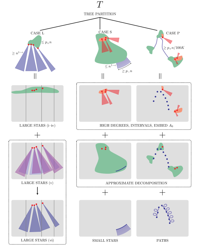
Figure 1: The three cases of the proof and the subroutines of the algorithm which embed each part of $T$. From left to right, Case L: almost all vertices lie in large stars; Case S: linearly many vertices lie in small stars; Case P: linearly many vertices lie in long bare paths. Red denotes high degree vertices and their neighbours. Blue denotes the part embedded in the exact step.

The heart of the approximate step algorithm is the subroutine APPROXIMATE DECOMPOSITION, where in each step we extend our partial embeddings $(\phi_{w}:w\in W)$ of $F$ by defining them on some set $A_{i}$ which is suitably nice: $A_{i}$ is independent, has linear size, has no vertices of degree $>n^{o(1)}$, and every vertex of $A_{i}$ has at most four previously embedded neighbours. We find these extensions simultaneously via a matching in an auxiliary hypergraph ${\cal H}_{i}$ (see Figure 2), which has an edge denoted $``\phi_{w}(u){=}x"$ whenever it is possible to define $``\phi_{w}(u){=}x"$ for some $w\in W$, $u\in A_{i}$, $x\in V=V(G)$. We encode the various constraints that must be satisfied by the embeddings in the definition of these edges. Thus $``\phi_{w}(u){=}x"$ includes (as an auxiliary vertex in $V({\cal H}_{i})$) all arcs $\overrightarrow{yx}$ where $y=\phi_{w}(b)$ is a previously defined embedding of some neighbour $b$ of $a$; this ensures that we maintain edge-disjointness of the embeddings of $F$. We also include in $``\phi_{w}(u){=}x"$ auxiliary vertices $uw$ and $xw$, to ensure that every $\phi_{w}(u)$ is defined at most once and $\phi_{w}$ is injective.

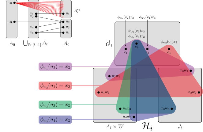
Figure 2: Part of the hypergraph $\mathcal{H}_{i}$, where a section of $F[A_{i},A_{<i}]$ and some of the corresponding edges of $\mathcal{H}_{i}$ are illustrated. Here, $u_{1}\in A^{\operatorname{hi}}_{i}$, $u_{2}\in A^{\operatorname{lo}}_{i}$ and $u_{3},u_{4}\in A^{\operatorname{no}}_{i}$. In a previous embedding, we set $\phi_{w_{1}}(v_{3})=\phi_{w_{3}}(v_{6})=x_{1}$, and now the arc $e_{2}=x_{3}x_{1}$ would be used by the potential embeddings $``\phi_{w_{1}}(u_{2})=x_{3}"$ (purple edge), $``\phi_{w_{3}}(u_{3})=x_{3}"$ (green edge) and $``\phi_{w_{3}}(u_{4})=x_{3}"$ (blue edge). In particular, at most one of these embeddings is allowed.

We ensure that ${\cal H}_{i}$ is suitably nice (its edges can be weighted so that every vertex has weighted degree $1+o(1)$ and all weighted codegrees are $n^{-o(1)}$), in which case it is well-known from the large literature developing Rödl’s semi-random ‘nibble’ [31], in particular [16], that one can find an almost perfect matching that is (in a certain sense) quasirandom (we use a convenient refined formulation of this statement recently presented in [8]). The quasirandomness of this matching is important for several reasons, including quasirandomness of the extensions of the embeddings to $A_{i}$, which in turn implies that later hypergraphs ${\cal H}_{j}$ with $j>i$ are suitably nice (with weaker specific parameters), and so the process can be continued.

The above sketch yields an alternative method for approximate decomposition results along the lines of those mentioned in the introduction, but has not yet dealt with high degree vertices. We will partition $V(F)$ into $A_{0},A_{1},\dots,A_{i^{*}}$, where $A_{i}$ for $i\geq 1$ are the nice sets described above, and $A_{0}$ is not nice – in particular, there is no bound on the degree of vertices in $A_{0}$. We start the embedding of $F$ in the subroutine HIGH DEGREES by embedding vertices sequentially in a suitable order, where when we consider some $a\in A_{0}$ we define $\phi_{w}(a)$ for all $w\in W$ simultaneously via a random matching $M_{a}=\{\phi_{w}(a)w:w\in W\}$ in an auxiliary bipartite graph $B_{a}\subseteq V\times W$, where the definition of $B_{a}$ encodes constraints that must be satisfied by the embedding: we only allow an edge $vw$ if $v\notin\operatorname{Im}\phi_{w}$ and $v$ is adjacent via unused edges to all $\phi_{w}(b)$ where $b$ is a previously embedded neighbour of $a$. (For simplicity we have suppressed several further details in the above description which will be discussed below.) The important point about this construction is that each $v\in V$ has to accommodate the vertex $a$ for a unique embedding $\phi_{w}$, so however large the degrees in $T$ may be, the total demand for ‘high degree edges’ is the same at every vertex, and can be allocated to a digraph $H$ which is an orientation of a quasirandom subgraph of $G$.

This digraph $H$ is one of many oriented quasirandom subgraphs into which $G$ is partitioned by the subroutine DIGRAPH, where each piece is reserved for embedding certain subgraphs of $F$, with arcs directed from earlier to later vertices. Besides $H$, these include graphs $G^{gg^{\prime}}_{ii^{\prime}}$ for embedding subgraphs $F^{\prime}[A^{g}_{i},A^{g^{\prime}}_{i^{\prime}}]$, according to a partition of each $A_{i}$ into $A^{\operatorname{hi}}_{i}$, $A^{\operatorname{lo}}_{i}$, $A^{\operatorname{no}}_{i}$. Here $A^{\operatorname{hi}}_{i}$ consists of vertices adjacent to some vertex with many neighbours in $A_{i}$ (which will lie in $A_{0}$ and be unique), $A^{\operatorname{lo}}_{i}$ consists of vertices adjacent to some vertex in $A_{0}$ (which will be unique) that does not have many neighbours in $A_{i}$, and $A^{\operatorname{no}}_{i}$ consists of vertices with no neighbours in $A_{0}$. To ensure concentration of probability the above sets are not defined if they would have size $o(n)$, in which case the corresponding vertices are instead added to $A_{0}$. By partitioning $G$ in this manner we can ensure edge-disjointness when embedding different parts of $F$ separately. To ensure injectivity of the embeddings, we also randomly partition $V\times W$ into various subgraphs in which $w$-neighbourhoods prescribe the allowed images in $\phi_{w}$ of the various parts of the decomposition of $V(T)$. In particular, while constructing the high degree digraph $H$, we also construct $J^{\operatorname{hi}}_{i}\subseteq V\times W$ so that each $\phi_{w}(A^{\operatorname{hi}}_{i})$ will be approximately equal to $J^{\operatorname{hi}}_{i}(w)$.

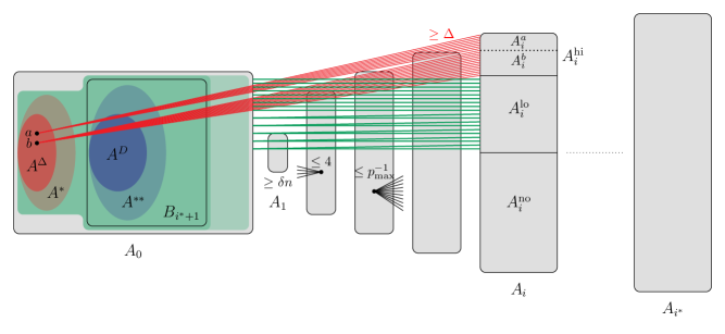
Figure 3: Partition of $F$ obtained in TREE PARTITION. Red edges are from $T\setminus F$ and green edges are $F$-edges from $A_{0}$ to $A_{i}$ (so $A^{\operatorname{lo}}_{i}$).

The separate treatment of these parts of $A_{i}$ and careful construction of $A_{0}$ to ensure the uniqueness properties mentioned above is designed to handle a considerable technical difficulty that we glossed over above when describing the embedding of $A_{0}$. Our approach to the approximate decomposition discussed above depends on maintaining quasirandomness, but we cannot ensure that $|A_{0}|/n$ is negligible compared with $1/i^{*}$, where $i^{*}$ is the number of steps in the approximate decomposition, so a naive analysis will fail due to blow-up of the error terms. We therefore partition $A_{0}$ into $A^{*}$, $A^{**}$ and $A^{\prime}_{0}$, which are embedded sequentially, where $|A^{*}|/n$ and $|A^{**}|/n$ are negligible compared with $1/i^{*}$, and so do not contribute much to the error terms. For $A^{\prime}_{0}$, we cannot entirely avoid large error terms, but we can confine them to a set of $o(n)$ bad vertices, via arguments based on Szemerédi regularity; these arguments require degrees in $A^{\prime}_{0}$ to be bounded independently of $n$, so $A^{**}$ is introduced to handle degrees that are $\omega(1)$ but $<n^{o(1)}$. The careful choice of partition ensures that these bad error terms are only incurred by vertices in $A^{\operatorname{lo}}$.

At this point, we return to consider various details glossed over in the above description of HIGH DEGREES. While the embedding via random matchings ensures that every vertex of $G$ has the same demand of high degree edges, we also need to plan ahead when embedding $A^{*}\subseteq A_{0}$ (which contains the very high degree vertices) so that it will be possible to allocate the other ends of these edges to distinct vertices for each $w$, i.e. so that $\phi_{w}(u)\neq\phi_{w}(u^{\prime})$ whenever $u\neq u^{\prime}$. To achieve this in DIGRAPH, we randomly partition $V$ into $(U_{h}:h\in[m])$, with $m=n^{1-o(1)}$, where each $U_{h}$ will accommodate those ends of high degree edges corresponding to colour $h$ in a certain properly $m$-edge-coloured bipartite multigraph in $V\times W$, i.e. $\overrightarrow{yx}$ is available for $H$ if $yw$ has colour $h$ and $x\in U_{h}$. Thus $x=\phi_{w}(u)\in U_{h}$ and $x^{\prime}=\phi_{w}(u^{\prime})\in U_{h^{\prime}}$ are distinct automatically if $h\neq h^{\prime}$, and due to properness of the colouring if $h=h^{\prime}$, as $c$ determines a unique $y\in V(G)$, so a unique $a=\phi_{w}^{-1}(y)\in A^{*}$.

The above multigraph $M$ in $V\times W$ consists of copies of $M^{*}_{a}\approx M_{a}$ for each $a\in A^{*}$, with the copies distinguished by labels $\ell_{aij}$, where for each $a\in A^{*}$ and part $A_{i}$ in which $a$ has many neighbours the number of labels $\ell_{aij}$ is proportional to the degree of $a$ in $A_{i}$. An edge $yw$ of label $\ell_{aij}$ in $M^{h}$ means that $H$ arcs $\overrightarrow{yx}$ with $x\in U_{h}$ will be allocated to edges $au$ of $F$ with $a=\phi_{w}^{-1}(y)$ and $u\in N_{F}(a)\cap A_{i}$. For typicality we require for any $a$ and $i$ that the number of edges in each $M^{h}$ with some label $\ell_{aij}$ is approximately independent of $h$.

This is achieved by a construction based on cyclic shifts, which we will now sketch, suppressing some details. We partition $V$ into $V_{0}$ and $(V_{v^{*}}:v^{*}\in V^{*})$ and $W$ into $W_{0}$ and $(W_{w^{*}}:w^{*}\in W^{*})$, where $V_{0}$ and $W_{0}$ are small, $V^{*}$ and $W^{*}$ are copies of $[m]$, and all $V_{v^{*}},W_{w^{*}}$ have the same size. The matchings $M_{a}$ are chosen as $M^{0}_{a}\cup M^{*}_{a}$, where $V(M^{0}_{a})=V_{0}\cup W_{0}$ and if $vw\in M^{*}_{a}$ then $v\in V_{v^{*}}$, $w\in W_{w^{*}}$ with $v^{*}=x_{a}+w^{*}$, according to some cyclic shifts $(x_{a}:a\in A^{*})$, carefully chosen to ensure edge-disjointness. We construct a labelled multigraph in $V^{*}\times W^{*}$ analogously to that in $V\times W$, and obtain label-balanced matchings $M^{h}$ for all $h\in[m]$ as cyclic shifts of some fixed label-balanced matching $M^{\prime}$ in $V^{*}\times W^{*}$, where for each $v^{*}w^{*}\in M^{\prime}$ with some label $\ell_{aij}$ we include in $M^{h}$ all edges of $M^{*}_{a}$ of the same label between $V_{v^{*}+h}$ and $W_{w^{*}+h}$.

The above description of $M^{h}$ is over-simplified, as in fact we construct two such matchings, one handling vertices of huge degree (almost linear) and the other handling vertices with degree that is high but not huge. The version of $M^{\prime}$ for non-huge degrees is constructed by the same hypergraph matching methods as in the above description of the approximate step embeddings, but these do not apply to huge degrees (the codegree bound fails) so we instead apply a result of Barát, Gyárfás and Sárközy [3] on rainbow matchings in properly coloured bipartite multigraphs. The construction is illustrated in Figure 4.

Figure 4: From left to right, top to bottom: two high degree vertices $a,b$; the multigraph $B^{\prime}_{\Delta}$ where line thickness represents multiplicity; the matchings $M_{a},M_{b}$ between $W$ and $V$; the matchings $M^{\prime}_{\Lambda},\mathcal{M}$ on $W^{*},V^{*}$; the matchings $M^{1}_{{\geq}\Lambda},M^{1}_{{<}\Lambda}$; the graph $D^{1}_{x}$ for $x\in U_{1}$ with components $P$ coloured to represent the random choice ${\operatorname{hi}}_{P}\in\{{\geq}\Lambda,{<}\Lambda\}$; the resulting edges of $H^{*}_{ai}$ at $x$.

The exact steps in Cases S and P are handled by adapting existing methods in the literature. In Case P, the subroutines INTERVALS and PATHS are adaptations of the methods we used in [20] for the ‘generalised Oberwolfach Problem’ of decomposing any quasirandom even regular oriented graph into prescribed cycle factors; we refer the reader to this paper for a detailed discussion of these methods. In Case S, we find the required stars by adapting an algorithm of [2]: we find an orientation of the unused graph so that the outdegree of each vertex is precisely the total size of stars it requires in all copies of $T$, and then process each vertex in turn, using random matchings to partition its outneighbourhood into stars of the correct sizes, while maintaining injectivity of the embeddings.

It remains to consider the exact step in Case L, when almost every vertex of $T$ is a leaf adjacent to a vertex of very large degree; this is more challenging and requires new methods (the arguments used in Case S fail due to lack of concentration of probability). The most difficult constraint to satisfy is injectivity of the embeddings, so we build this into the construction explicitly: we randomly partition $V(G)$ into sets $U^{a}$ for each star centre $a$ and require each embedding to choose most of its leaves for its copy of $a$ within $U^{a}$. Each edge $xy$ of $G$, say with $x\in U^{a}$, $y\in U^{b}$, will be randomly allocated one of two options: (i) $x$ is a leaf of a star in some embedding $\phi_{w}$ with $\phi_{w}(a)=y$, or (ii) $y$ is a leaf of a star in some embedding $\phi_{w^{\prime}}$ with $\phi_{w^{\prime}}(b)=x$. A final balancing step will swap edges between stars (thus slightly bending the rules on leaf allocation) so that all stars are exactly as required; see Figure 5. The above sketch can be implemented for decomposing a quasirandom graph into star forests, but there is a considerable extra difficulty caused by the constraints imposed by the initial embedding of the small part of $T$ not contained in the large stars.

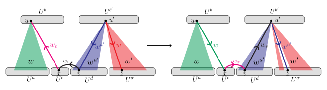
Figure 5: A single step of the algorithm to modify the green star which is too small and the red star which is too large.

A naive approach to this embedding can easily cause many edges of $G$ to be unusable according to the rules for $U^{a}$ as described above. Indeed, for each edge $xy$ of $G$, the two options as described above will both become unavailable during the initial embedding if we choose both $\phi_{w}(a^{\prime})=x$ for some $a^{\prime}$ and $\phi_{w^{\prime}}(b^{\prime})=y$ for some $b^{\prime}$. We therefore keep track of a digraph $J$ that records these constraints and choose the initial embedding so that each edge of $G$ always has at least one of its two options available. To control these constraints, we also introduce partitions of each $U^{a}$ into three parts, and also of the set $W$ indexing the embeddings into three parts, and impose two different patterns for matching parts of $U^{a}$ with parts of $W$ according to whether or not a vertex has large degree. The digraph $J$ and its use in defining available sets for the embedding are illustrated in Figure 6.

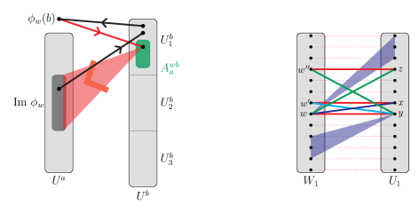
Figure 6: (Left) the available set $A^{wb}_{a}$ for $w\in W_{1}$ and $a\in S$. The black arcs are some arcs in $J$; they forbid their $U^{b}$-endvertices from $A^{wb}_{a}$. The red arcs would be added to $J$ if the labelled vertex is chosen for $\phi_{w}(a)$. (Right) A pair of edges $wy$, $w^{\prime}x$ that must be avoided by the matching defining the embeddings of $a$, and a swap that may be implemented by Lemma 2.7 to remove $wy$. Red edges define images of $a$ and blue edges define images of some other vertices.

2.1 Formal statement of the algorithm

The input to the algorithm consists of a $(\xi,s)$-typical graph $G$ on $n$ vertices of density $p$, where $s=2^{50\cdot 8^{3}}$, $n^{-1}\ll\xi\ll p$, and a tree $T$ with $p(n-1)/2$ edges. We fix $0<c^{\prime}\ll c\ll 1$ and parameters

$$n^{-1}\ll\xi\ll\eta_{-}\ll p_{-}\ll\eta_{+}\ll p_{+}\ll p,\quad\text{ and }\Delta=n^{c},\ \Lambda=n^{1-c}.$$

Recall that a leaf in $T$ is a vertex of degree $1$ in $T$. We call an edge a leaf edge if it contains a leaf. We call a star a leaf star if it consists of leaf edges. We call a path in $T$ a $k$-path if it has length $k$ (that is, $k$ edges), and call it bare if its internal vertices all have degree $2$ in $T$. By Lemma 2.9 below we can choose a case for $T$ in {L,S,P} satisfying

• Case L: all but at most $p_{+}n$ vertices of $T$ belong to leaf stars of size ${\geq}\Lambda$,

• Case S: at least $p_{-}n$ vertices of $T$ belong to leaf stars of size $\leq\Lambda$,

• Case P: $T$ contains $p_{+}n/100K$ vertex-disjoint bare $8K$-paths.

In Case L go to LARGE STARS, otherwise continue. We let $\eta=\eta_{-}$ in Case S or $\eta=\eta_{+}$ in Case P, and define further parameters

$$\xi\ll\xi^{\prime}\ll D^{-1}\ll\delta\ll p_{\min}\ll\varepsilon_{1}\ll\ldots\ll\varepsilon_{i^{+}}\ll p_{\rm{max}}\ll\varepsilon\ll p_{0}\ll\eta\ll s^{-1},p,$$

with $i^{+}=7\log\varepsilon^{-1}$ and $\xi^{\prime}\ll K^{-1}\ll d^{-1}\ll D^{-1}$ in Case P. Given $k\in\mathbb{N}$, a tree $T$ and $S\subseteq V(T)$, the $k$-span $\text{span}^{k}_{T}(S)$ of $S$ in $T$ is obtained by starting with $S^{*}=S$ and iteratively adding any $S^{\prime}\subseteq V(T)\setminus S^{*}$ with $|S^{\prime}|\in[k]$ such that $T[S^{*}\cup S^{\prime}]$ has fewer components than $T[S^{*}]$, until there is no such $S^{\prime}$. Clearly there are at most $|S|$ iterations, so $|\text{span}^{k}_{T}(S)|\leq(k+1)|S|$. Note also that $|\text{span}^{k}_{T}(\text{span}^{k}_{T}(A)\cup B)\setminus\text{span}^{k}_{T}(A)|\leq(k+1)|B|$. For $k\in\mathbb{N}$ let $A^{k}=\{u:d_{T}(u)\geq k\}$.

TREE PARTITION

1. Let $A^{*}=\text{span}^{4}_{T}(A^{\Delta})$. In Case S let $P_{\operatorname{ex}}$ be a union of leaf stars in $T\setminus T[A^{*}]$, each of size $\leq\Lambda$, with $|P_{\operatorname{ex}}|=p_{-}n/2\pm\Lambda$. In Case P let $P_{\operatorname{ex}}$ be the vertex-disjoint union of two leaf edges in $T\setminus T[A^{*}]$ and $p_{+}n/101K$ bare $8K$-paths in $T\setminus T[A^{*}]$.
   Obtain $F$ from $T$ by deleting all edges of $P_{\operatorname{ex}}$ and $F^{*}$ from $F$ by deleting all vertices of $A^{*}$.

2. Define disjoint independent sets $C_{1},\dots,C_{i^{*}}$ in $F^{*}$ as follows. At step $i\geq 1$, let $B_{i}=V(F^{*})\setminus\bigcup_{j<i}C_{j}$, let $C^{\prime}_{i}$ be the set of $v\in B_{i}$ with $d_{F^{*}[B_{i}]}(v)\leq 3$ and $d_{F^{*}[\bigcup_{j<i}C_{j}]}(v)\leq p_{\rm{max}}^{-1}$, and let $C_{i}$ be a maximum independent set in $F^{*}[C^{\prime}_{i}]$. If $|C_{i}|<\varepsilon n$ let $i^{*}=i-1$ and stop, otherwise go to the next step.

3. Let $A_{0}=\text{span}^{4}_{T}[A^{*}\cup B_{i^{*}+1}]$. Let $A^{**}=\text{span}^{4}_{T}(A^{D})\setminus A^{*}$ and $A^{\prime}_{0}=A_{0}\setminus(A^{*}\cup A^{**})$.
   For $i\in[i^{*}]$ let $A_{i}=C_{i^{*}+1-i}\setminus A_{0}$ and for $k\in\mathbb{N}$ let $A^{k}_{i}=\{a\in A^{k}:|N_{F}(a)\cap A_{i}|\geq\Delta\}$.
   For $a\in A^{\Delta}_{i}$ let $A^{a}_{i}=N_{F}(a)\cap A_{i}$. Let $A^{\operatorname{hi}}_{i}=\bigcup_{a\in A^{\Delta}_{i}}A^{a}_{i}$ and $A^{{<}\Lambda}_{i}=\bigcup_{a\in A^{\Delta}_{i}\setminus A^{\Lambda}_{i}}A^{a}_{i}$ and $A^{{\geq}\Lambda}_{i}=\bigcup_{a\in A^{\Lambda}_{i}}A^{a}_{i}$. Obtain $F^{\prime}$ from $F$ by deleting all edges $ab$ with $a\in A^{\Delta}_{i}$ and $b\in A^{a}_{i}$ for some $i$. Let $A^{\operatorname{lo}}_{i}=\{u\in A_{i}:|N_{F^{\prime}}(u)\cap A_{0}|=1\}$. Let $A^{\operatorname{no}}_{i}=\{u\in A_{i}:N_{F}(u)\cap A_{0}=\emptyset\}$.

4. For $j\in[4]$, let $\delta_{j}=\delta^{.1j+.6}$ and let $(\circ_{1},\ldots,\circ_{4})=(\operatorname{no},{\geq}\Lambda,{<}\Lambda,\operatorname{lo})$. For each $j\in[4]$, while any $|A^{\circ_{j}}_{i}|<\delta_{j}n$ move $A^{\circ_{j}}_{i}$ to $A_{0}$, let $A_{0}=\text{span}^{4}_{T}[A_{0}\cup A^{\circ_{j}}_{i}]$, and update $A^{{<}\Lambda}_{i},A^{{\geq}\Lambda}_{i},A^{\operatorname{lo}}_{i},A^{\operatorname{no}}_{i}$.

5. If $\bigcup_{i}A^{\operatorname{hi}}_{i}=\emptyset$ move $A^{*}$ to $A^{**}$, i.e. redefine $A^{**}$ as $A^{**}\cup A^{*}$ and $A^{*}$ as $\emptyset$.

Let $A^{\operatorname{hi}}=\bigcup_{i}A^{\operatorname{hi}}_{i}$ and define $A^{\operatorname{no}},A^{\operatorname{lo}}$ similarly.

For $k\in\mathbb{N}$, let $Q^{\Delta}=\{(a,i):\Delta\leq|N_{F}(a)\cap A_{i}|<\Lambda\}\subseteq A^{\Delta}\times[i^{*}]$ and $Q^{\Lambda}=\{(a,i):|N_{F}(a)\cap A_{i}|\geq\Lambda\}\subseteq A^{\Lambda}\times[i^{*}]$. We introduce parameters

$$m^{a}_{i}=\left\lceil\Delta^{-.2}|A^{a}_{i}|\right\rceil 1_{a\in A^{\Delta}_{i}},\quad m_{a}=\sum_{i}m^{a}_{i},\quad m=\sum_{a\in A^{\Delta}}m_{a}.$$

Let $\prec$ be an order on $V(T)$ with $A^{*}\prec A^{**}\prec A^{\prime}_{0}\prec A_{1}\prec\dots\prec A_{i^{*}}\prec V(P_{\operatorname{ex}})\setminus V(T)$ and $|N_{<}(v)\cap X|\leq 1$ whenever $v\in X\in\{A^{*},A^{**},A^{\prime}_{0}\}$. For $v\in V(T)$ we let ${<}v=\{u:u\prec v\}$, $N_{<}(v)=N_{F^{\prime}}(v)\cap{<}v$, $N_{\leq}(v)=N_{<}(v)\cup\{v\}$ and $N_{>}(v)=N_{F^{\prime}}(v)\setminus{<}v$.

We stress the use of $F^{\prime}$ in this notation, which ensures that $N_{>}(a)\cap A^{\operatorname{hi}}_{i}=\emptyset$ for all $a\in A_{0}$: otherwise we would have a vertex not in $A_{0}$ adjacent to two vertices of $A_{0}$, but this contradicts the definition of $A_{0}$ as a span. We list here some other immediate consequences of the definition of $A_{0}$ that will often be used without comment.

• $|A^{*}|\leq 5n/\Delta$ and $|A^{**}|\leq 5n/D$.

• Any $u\in A_{\geq 1}$ has $|N_{<}(u)\cap A_{0}|\leq 1$.

• Any $uv\in F[A_{\geq 1}]$ has $|(N_{<}(u)\cup N_{<}(v))\cap A_{0}|\leq 1$.

• There is no ${\leq}3$-path in $T\setminus A_{0}$ with both ends in $A^{\operatorname{hi}}\cup A^{\operatorname{lo}}$.

We also note that $|N_{>}(v)|\leq p_{\rm{max}}^{-1}$ for all $v\in A_{\geq 1}$, and $|N_{<}(v)|\leq 4$ for all $v\in V(T)$. To see the latter, note that if $v\in A_{\geq 1}$ then $v$ has at most $3$ earlier neighbours in $A_{\geq 1}$ and at most one in $A_{0}$, whereas if $v\in A_{0}$ then $v$ has at most one earlier neighbour in each of $A^{*}$, $A^{**}$ and $A^{\prime}_{0}$.

Write $n=mn_{*}+n_{0}$ with $|n_{0}-n\Delta^{-.1}|<m$. Recall that we adopt the natural cyclic orders on $[m]$ and $[n]$, addition wraps, and $d(\cdot,\cdot)$ is cyclic distance. Whenever an algorithm is required to make a choice, it aborts if it is unable to do so (we will show whp it does not abort).

Given bipartite graphs $B,Z\subseteq X\times Y$ with $|X|=|Y|$ we write $M{=}$MATCH$(B,Z)$ to mean that $M$ is a random perfect matching from Lemma 2.7. (The choice of $Z$ will ensure edge-disjointness of the embeddings.)

HIGH DEGREES

1. Choose $x_{a}\in[m]$ for $a\in A^{*}$ in $\prec$ order, arbitrarily subject to $d(x_{a},x_{a^{\prime}})>3d$ for all $a^{\prime}\prec a$, and $d(x_{a},x_{a^{\prime}})\neq d(x_{b},x_{b^{\prime}})$ for all $a^{\prime}\in N_{<}(a)$ and $bb^{\prime}\in F[{<}a]$.

2. Choose independent uniformly random partitions of $V(G)$ into $V_{0}$ of size $n_{0}$ and $V_{v^{*}}$, $v^{*}\in V^{*}$ of size $n_{*}$, and $W$ into $W_{0}$ of size $n_{0}$ and $W_{w^{*}}$, $w^{*}\in W^{*}$ of size $n_{*}$, where $V^{*}=W^{*}=[m]$.

3. For each $a\in A^{*}$ in $\prec$ order we will define all $\phi_{w}(a)$ by choosing a perfect matching $M_{a}=\{\phi_{w}(a)w:w\in W\}$. Let $B_{a}\subseteq V\times W$ consist of all $vw$ where $v\notin\operatorname{Im}\phi_{w}$ and each $\phi_{w}(b)v$ with $b\in N_{<}(a)$ is an unused edge of $G$. Let $Z_{a}\subseteq V\times W$ consist of all $\phi_{w}(b)w$ with $b\in N_{<}(a)$.
   Let $B^{0}_{a}=B_{a}[V_{0},W_{0}]$ and $B^{w^{*}}_{a}=B_{a}[V_{x_{a}+w^{*}},W_{w^{*}}]$ for $w^{*}\in W^{*}$. Define $Z^{0}_{a}$ and $Z^{w^{*}}_{a}$ similarly.
   Let $M_{a}=M^{0}_{a}\cup M^{*}_{a}$ with $M^{0}_{a}{=}$MATCH$(B^{0}_{a},Z^{0}_{a})$ and $M^{*}_{a}{=}\bigcup_{w^{*}}$MATCH$(B^{w^{*}}_{a},Z^{w^{*}}_{a})$.

We randomly identify $V(G)$ with $[n]$, cyclically ordered as above. Recall that each $x\in[n]$ has successor $x^{+}=x+1$ (where $n+1$ means $1$) and predecessor $x^{-}=x-1$ (where $0$ means $n$). Let $d_{i}=d/(2s)^{i-1}$ for $i\in[2s+1]$. We write $n=r_{i}d_{i}+s_{i}$ with $r_{i}\in\mathbb{N}$ and $0\leq s_{i}<d_{i}$, and let

$$P^{i}_{j}=\left\{\begin{array}[]{ll}\{kd_{i}+j:0\leq k\leq r_{i}\}&\text{if }j\in[s_{i}],\\ \{kd_{i}+j:0\leq k\leq r_{i}-1\}&\text{if }j\in[d_{i}]\setminus[s_{i}].\end{array}\right.$$

For each $i\in[s+1]$ and $j\in[d_{i}]$ we define a partition of $[n]$ into a family of cyclic intervals $\mathcal{I}^{i}_{j}$ defined as all $[x,y^{-}]$ where $x\in P^{i}_{j}$ and $y$ is the next element of $P^{i}_{j}$ in the cyclic order. (So $|\mathcal{I}^{i}_{j}|=n/d_{i}\pm 1$, each $I\in\mathcal{I}^{i}_{j}$ has $|I|\leq d_{i}$, and $\mathcal{I}^{i}_{j}\cap\mathcal{I}^{i}_{j^{\prime}}=\emptyset$ for $j\neq j^{\prime}$.) We let $\mathcal{I}^{i}=\bigcup_{j\in[d_{i}]}\mathcal{I}^{i}_{j}$. (So for every $z\in[n]$, exactly one $[x,y^{-}]\in\mathcal{I}^{i}$ has $x=z$, and exactly one $[x,y^{-}]\in\mathcal{I}^{i}$ has $y=z$.)

INTERVALS

1. In Case S let $\overline{X}_{\!\!w}=V\setminus\phi_{w}(A^{*})$, $\overline{p}_{w}:=n^{-1}|\overline{X}_{\!\!w}|$ for all $w\in W$ and go to DIGRAPH; otherwise (in Case P) continue. For each $w\in W$ independently choose $i(w)\in[2s+1]$ and $j(w)\in[d_{i(w)}]$ uniformly at random. Let $W_{i}=\{w:i(w)=i\}$.

2. For each $w\in W$, let $\mathcal{A}_{w}$ include each interval of $\mathcal{I}^{i(w)}_{j(w)}$ independently with probability $1/2$.
   Let $\mathcal{S}_{w}$ consist of all $I\in\mathcal{A}_{w}$ such that both neighbouring intervals $I^{\pm}$ of $I$ are not in $\mathcal{A}_{w}$.

3. For each $w\in W$, let $\mathcal{X}_{w}$ include each $I\in\mathcal{S}_{w}$ with probability $(1-\eta)n^{-1}|P_{\operatorname{ex}}|$ independently, let $X_{w}=\bigcup\mathcal{X}_{w}$, $\overline{X}_{\!\!w}=V\setminus(\phi_{w}(A^{*})\cup X_{w}\cup(X_{w})^{+})$ and $\overline{p}_{w}=n^{-1}|\overline{X}_{\!\!w}|$.

4. Obtain $\mathcal{Y}_{w}\subseteq\mathcal{X}_{w}$ as follows. Remove any $I$ from $\mathcal{X}_{w}$ that intersects $\phi_{w}(A^{*})$, let $t_{i}=\min\{|\mathcal{X}(I)|:I\in\mathcal{I}^{i}\}$, where $\mathcal{X}(I):=\{w\in W_{i}:I\in\mathcal{X}_{w}\}$, then delete each $I\in\mathcal{I}^{i}$, $i\in[2s+1]$ from $|\mathcal{X}(I)|-t_{i}$ sets $\mathcal{X}_{w}$ with $w\in\mathcal{X}(I)$, independently uniformly at random.
   Let $Y_{w}=\bigcup\mathcal{Y}_{w}$ and $\mathcal{Y}(I)=\{w\in W_{i}:I\in\mathcal{Y}_{w}\}$.

EMBED $A_{0}$

1. For each $xy\in G^{*}:=G\setminus\bigcup_{w}\phi_{w}(T[A^{*}])$ independently let $\mathbb{P}(xy\in G_{0})=p_{0}/p$.
   For each $w\in W$ and $x\in\overline{X}_{\!\!w}$ independently let $\mathbb{P}(\overrightarrow{xw}\in J_{0})=p_{0}/\overline{p}_{w}$.

2. Extend the embeddings $\phi_{w}$ of $T[A^{*}]$ to $T[A_{0}]$ in $\prec$ order, where for each $a\in A_{0}\setminus A^{*}$ we choose a perfect matching $M_{a}=\{\phi_{w}(a)w:w\in W\}{=}$MATCH$(B_{a},Z_{a})$, where $Z_{a}=\{\phi_{w}(b)w:b\in N_{<}(a)\}$ and $B_{a}\subseteq V\times W$ consists of all $vw$ with $v\in N_{J_{0}}(w)\setminus\operatorname{Im}\phi_{w}$ where each $\phi_{w}(b)v$ with $b\in N_{<}(a)$ is an unused edge of $G_{0}$.

For $i,i^{\prime}\in[i^{*}]$ and $g,g^{\prime}\in\{\operatorname{hi},\operatorname{lo},\operatorname{no}\}$, let $p^{gg^{\prime}}_{ii^{\prime}}=n^{-1}|F^{\prime}[A^{g}_{i},A^{g^{\prime}}_{i^{\prime}}]|+p_{\min}$ and $p^{g}_{i0}=n^{-1}|F^{\prime}[A^{g}_{i},A_{0}]|+p_{\min}$. We also write $p^{gg^{\prime}}_{i0}=p^{g}_{i0}$ for all $g^{\prime}$ for uniform notation later.

For $i\in[i^{*}]$, $g\in A^{\Delta}_{i}\cup\{\operatorname{lo},\operatorname{no}\}$ let $\alpha^{g}_{i}=|A^{g}_{i}|n^{-1}$, $\alpha_{\operatorname{lo}}=|A^{\operatorname{lo}}|n^{-1}$, $\alpha_{\operatorname{no}}=|A^{\operatorname{no}}|n^{-1}$ and $\alpha_{0}=|A_{0}|n^{-1}$.

Let $\alpha^{\operatorname{hi}}_{i}=\Delta^{.2}m_{i}/n$ and $\alpha_{\operatorname{hi}}=\sum_{i}\alpha^{\operatorname{hi}}_{i}=\Delta^{.2}m/n=|A^{\operatorname{hi}}|n^{-1}\pm\Delta^{-.9}$.

Let $p_{\operatorname{ex}}=n^{-1}|P_{\operatorname{ex}}|$. Let $p^{\prime}_{\operatorname{ex}}=(\tfrac{7}{8}-\eta)p_{\operatorname{ex}}$ in Case P or $p_{\operatorname{ex}}\ll p^{\prime}_{\operatorname{ex}}\ll 1$ in Case S.

We note some identities and estimates for our parameters:

$$p(n-1)/2=|T|=|T[A_{0}]|+|F^{\prime}|+|A^{\operatorname{hi}}|+|P_{\operatorname{ex}}|,$$

$$1+p(n-1)/2=|V(T)|=|V(F)|+|V(P_{\operatorname{ex}})\setminus V(F)|,$$

$$\sum_{i,i^{\prime},g,g^{\prime}}p^{gg^{\prime}}_{ii^{\prime}}-n^{-1}|F^{\prime}|\in[0,{p_{\min}}^{.9}],\quad\sum_{i}\alpha^{g}_{i}=n^{-1}|A^{g}|,$$

$$p/2-\sum p^{gg^{\prime}}_{ii^{\prime}}-\alpha_{\operatorname{hi}}-p_{\operatorname{ex}}\in[0,{p_{\min}}^{.9}],\quad p/2-(\alpha_{\operatorname{hi}}+\alpha_{\operatorname{lo}}+\alpha_{\operatorname{no}}+p_{\operatorname{ex}})\in[0,\varepsilon^{.9}],$$

$$\overline{p}_{w}=\begin{cases}1-|A_{0}|n^{-1}\text{ in Case S, or }\\ \overline{p}\pm d^{-.9}\text{ with }\overline{p}=(1-\alpha_{0})(1-(1-\eta)p_{\operatorname{ex}}/8)\text{ in Case P}.\end{cases}$$

These estimates imply that the assignment of probabilities to mutually exclusive events in DIGRAPH.vii below are valid (i.e. have sum $\leq 1$). For $\circ\in\{{<}\Lambda,{\geq}\Lambda\}$, let

$$m_{\circ}=\sum_{(a,i)\in Q^{\circ}}m^{a}_{i},\quad p_{\circ}=m_{\circ}/m,\quad\text{and define}$$

$$\text{ labels }L_{\circ}=\{\ell_{aij}:(a,i)\in Q^{\circ},j\in[M^{a}_{i}]\},\text{ where }M^{a}_{i}\in\left\{\left\lfloor m^{a}_{i}/p_{\circ}\right\rfloor,\left\lceil m^{a}_{i}/p_{\circ}\right\rceil\right\}\quad\text{and }|L_{\circ}|=m.$$

DIGRAPH

1. For each $a\in A^{\Delta}$ let $M^{\prime}_{a}$ denote the perfect matching between $V^{*}$ and $W^{*}$ consisting of all $v^{*}w^{*}$ with $w^{*}\in W^{*}$ and $v^{*}=x_{a}+w^{*}\in V^{*}$. Let $B^{\prime}_{ai}$ be the bipartite multigraph formed by $M^{a}_{i}$ copies of $M^{\prime}_{a}$ labelled by $\ell_{aij}$, $j\in[M^{a}_{i}]$. For $k\in\mathbb{N}$ let $B^{\prime}_{k}=\bigcup_{(a,i)\in Q^{k}}B^{\prime}_{ai}$ and $B_{k}$ be the bipartite multigraph formed by $M^{a}_{i}$ copies of $M^{*}_{a}$ for each $(a,i)\in Q^{k}$ labelled by $\ell_{aij}$, $j\in[M^{a}_{i}]$.

2. Let $M^{\prime}_{\Lambda}$ be a largest matching in $B^{\prime}_{\Lambda}$ with at most one edge of each label. Define a partial $m$-edge-colouring $(M^{h}_{{\geq}\Lambda}:h\in[m])$ of $B_{\Lambda}$, where for each $h\in[m]$ and edge $v^{*}w^{*}$ of $M^{\prime}_{\Lambda}$ with some label $\ell_{aij}$ we include in $M^{h}_{{\geq}\Lambda}$ all edges of $M^{*}_{a}$ with label $\ell_{aij}$ between $V_{v^{*}+h}$ and $W_{w^{*}+h}$.

3. Let $({\cal H},\omega)$ be the weighted $3$-graph where for each $v^{*}w^{*}$ labelled $\ell_{aij}$ with $(a,i)\in Q^{\Delta}$ we include $v^{*}w^{*}\ell_{aij}$ with weight $m^{-1}$. Let ${\cal M}$ be a random matching obtained from Lemma 2.8 applied to $({\cal H},\omega)$. Define matchings $M^{h}_{{<}\Lambda}\subseteq B_{\Delta}$ for $h\in[m]$, where for each edge $v^{*}w^{*}\ell_{aij}$ of ${\cal M}$ we include in $M^{h}_{{<}\Lambda}$ all edges of $M^{*}_{a}$ with label $\ell_{aij}$ between $V_{v^{*}+h}$ and $W_{w^{*}+h}$.

4. Partition $V$ as $(U_{h}:h\in[m])$ uniformly at random. Fix distinct $h_{aij}\in[m]$ for each $\ell_{aij}\in L_{\circ}$ and $\circ\in\{{<}\Lambda,{\geq}\Lambda\}$ (recalling $|L_{\circ}|=m$). For all $\ell_{aij}\in L_{\circ}$, add a copy of $M^{0}_{a}$ with every edge labelled $\ell_{aij}$ to $M^{h_{aij}}_{\circ}$. Let $p_{1}=p-p_{0}$ and $\overrightarrow{G}_{1}$ be a uniformly random orientation of $G_{1}:=G^{*}\setminus(G_{0}\cup\{xy:d(x,y)\geq 3d\})$.

5. For $h\in[m]$ and $x\in U_{h}$ let $D^{h}_{x}$ be the graph on $N^{-}_{\overrightarrow{G}_{1}}(x)$ consisting of all $yy^{\prime}$ with $y\neq y^{\prime}$ such that $yw\in M^{h}_{{\geq}\Lambda}$ and $y^{\prime}w\in M^{h}_{{<}\Lambda}$ for some $w\in W$ with $x\in\overline{X}_{\!\!w}$. For each connected component $P$ of $D^{h}_{x}$ independently choose one of $\mathbb{P}(\operatorname{hi}_{P}=\circ)=p_{\circ}$ for $\circ\in\{{\geq}\Lambda,{<}\Lambda\}$. For each $y\in P$ with some $yw\in M^{h}_{\operatorname{hi}_{P}}$ with label $\ell_{aij}$ include $\overrightarrow{yx}$ in $H^{*}_{ai}$ and let $w(\overrightarrow{yx})=w$.

6. For each $\overrightarrow{yx}\in\overrightarrow{G}_{1}$ independently choose at most one of $\mathbb{P}(\overrightarrow{yx}\in\overrightarrow{G}_{\operatorname{ex}})=2p_{\operatorname{ex}}/p_{1}$ or $\mathbb{P}(\overrightarrow{yx}\in\overrightarrow{G}^{gg^{\prime}}_{ii^{\prime}})=2p^{gg^{\prime}}_{ii^{\prime}}/p_{1}$ for $1\leq i^{\prime}<i\leq i^{*}$ and $g,g^{\prime}\in\{\operatorname{hi},\operatorname{lo},\operatorname{no}\}$, or $\mathbb{P}(\overrightarrow{yx}\in\overrightarrow{G}^{g}_{i0})=2p^{g}_{i0}/p_{1}$ for $i\in[i^{*}]$ and $g\in\{\operatorname{hi},\operatorname{lo},\operatorname{no}\}$, or $\mathbb{P}(\overrightarrow{yx}\in\overrightarrow{G}^{\prime}_{i})=2p_{\rm{max}}/p_{1}$ for $i\in[i^{*}]$, or $\mathbb{P}(\overrightarrow{yx}\in H)=2\alpha_{\operatorname{hi}}/p_{1}\overline{p}_{w}$ if $x\in\overline{X}_{\!\!w}$, where $w=w(\overrightarrow{yx})$, and if $\overrightarrow{yx}\in H^{a}_{i}:=H\cap H^{*}_{ai}$ include $\overrightarrow{xw}\in J^{a}_{i}$. Let $J^{\operatorname{hi}}_{i}=\bigcup_{a\in A^{\Delta}_{i}}J^{a}_{i}$ and $J^{\operatorname{hi}}=\bigcup_{i}J^{\operatorname{hi}}_{i}$ and $\overrightarrow{G}_{i}=\bigcup_{g,g^{\prime},j}\overrightarrow{G}^{gg^{\prime}}_{ij}$.

7. Let $J^{\prime}$ be the set of $\overrightarrow{xw}\notin J_{0}\cup J^{\operatorname{hi}}$ with $x\in\overline{X}_{\!\!w}$. For $\overrightarrow{xw}\in J^{\prime}$ let $p_{xw}=\overline{p}_{w}p_{1}-2\alpha_{\operatorname{hi}}\operatorname{hi}_{xw}$, where $\operatorname{hi}_{xw}$ is $1$ if $w=w(\overrightarrow{yx})$ for some $y$ or $0$ otherwise. For each $\overrightarrow{xw}\in J^{\prime}$ independently choose at most one of $\mathbb{P}(\overrightarrow{xw}\in J_{\operatorname{ex}})=p^{\prime}_{\operatorname{ex}}/p_{xw}$ or $\mathbb{P}(\overrightarrow{xw}\in J^{\operatorname{lo}}_{i})=\alpha^{\operatorname{lo}}_{i}/p_{xw}$ or $\mathbb{P}(\overrightarrow{xw}\in J^{\operatorname{no}}_{i})=\alpha^{\operatorname{no}}_{i}/p_{xw}$ or $\mathbb{P}(\overrightarrow{xw}\in J^{\prime}_{i})=p_{\rm{max}}/p_{xw}$. Let $J^{\operatorname{lo}}=\bigcup_{i}J^{\operatorname{lo}}_{i}$ and $J^{\operatorname{no}}=\bigcup_{i}J^{\operatorname{no}}_{i}$.

8. In Case P, for each $\overrightarrow{yx}\in\overrightarrow{G}_{\operatorname{ex}}$ independently let $\mathbb{P}(\overrightarrow{yx}\in J^{0}_{\operatorname{ex}})=\tfrac{7}{8}$ or $\mathbb{P}(\overrightarrow{yx}^{-}\in J^{K}_{\operatorname{ex}})=\tfrac{1}{8}$.

Some edges of $G$ may not be allocated by this process. Note that arcs in $J[V,W]$ are all directed from $V$ to $W$, so we will often suppress the direction and think of $J[V,W]$ as a graph.

For $uu^{\prime}\in F^{\prime}[A^{g}_{i},A^{g^{\prime}}_{i^{\prime}}]$ with $i,i^{\prime}\in[0,i^{*}]$ and $g,g^{\prime}\in\{\operatorname{hi},\operatorname{lo},\operatorname{no}\}$ let every $\overrightarrow{G}^{gg^{\prime}}_{i0}=\overrightarrow{G}^{g}_{i0}$ and let $\overrightarrow{G}_{uu^{\prime}}=\overrightarrow{G}^{gg^{\prime}}_{ii^{\prime}}$ and $p_{uu^{\prime}}=p^{gg^{\prime}}_{ii^{\prime}}$, recalling that $p^{gg^{\prime}}_{i0}=p^{g}_{i0}$ for all $g^{\prime}$.

For $g\in A^{\Delta}\cup\{\operatorname{lo},\operatorname{no}\}$, $u\in A^{g}_{i}$ let $A_{u}=A^{g}_{i}$, $J_{u}=J^{g}_{i}$, $\alpha_{u}=\alpha^{g}_{i}$.

For $\overrightarrow{xw}\in J_{u}$ we also write $A_{\overrightarrow{xw}}=A_{u}$, $J_{\overrightarrow{xw}}=J_{u}$, $\alpha_{\overrightarrow{xw}}=\alpha_{u}$.

APPROXIMATE DECOMPOSITION

For $i=1,\dots,i^{*}$ apply the following steps.

1. Let $({\cal H}_{i},\omega)$ be the weighted hypergraph ${\cal H}_{i}$ with vertex parts $\overrightarrow{G}_{i}$, $J_{i}$ and $A_{i}\times W$, where for each $u\in A_{i}$ and $\overrightarrow{xw}\in J_{u}$ such that $\overleftarrow{xy}\in\overrightarrow{G}_{uv}$ for all $y=\phi_{w}(v)$ with $v\in N_{<}(u)$ we include an edge labelled $``\phi_{w}(u){=}x"$ consisting of $uw$, $\overrightarrow{xw}$ and all such $\overleftarrow{xy}$, with weight

   $$\omega(``\phi_{w}(u){=}x"):=|A_{u}|^{-1}\prod_{v\in N_{<}(u)}p_{uv}^{-1}.$$

2. Define $\omega^{\prime}$ on ${\cal H}_{i}$ by $\omega^{\prime}(\bm{e})=(1-.5\varepsilon_{i})\omega(\bm{e})/Q(\bm{e})$ where $Q(\bm{e})$ is the maximum of $1$ and all $\omega({\cal H}_{i}[\bm{v}]):=\sum\{\omega(\bm{e}):\bm{v}\in\bm{e}\}$ with $\bm{v}\in\bm{e}$. Let ${\cal M}_{i}$ be a random matching obtained by applying Lemma 2.8 to $({\cal H}_{i},\omega^{\prime})$. For each $``\phi_{w}(u){=}x"$ in ${\cal M}_{i}$ extend $\phi_{w}$ by setting $\phi_{w}(u)=x$.

3. For each $a\in A_{i}$ in any order, let $W_{a}=\{w\in W:\phi_{w}(a)$ undefined$\}$, let $V_{a}\in\tbinom{V}{|W_{a}|}$ be uniformly random, and define $\{\phi_{w}(a)w:w\in W_{a}\}{=}$MATCH$(B_{a},Z_{a})$, where $Z_{a}=\{\phi_{w}(b)w:b\in N_{<}(a)\}$ and $B_{a}\subseteq V_{a}\times W_{a}$ consists of all $vw$ with $v\in N_{J^{\prime}_{i}}(w)\setminus\operatorname{Im}\phi_{w}$ and each $\phi_{w}(b)v$ for $b\in N_{<}(a)$ an unused edge of $G^{\prime}_{i}$.

To avoid confusion, we emphasise that $H_{i}$ is a digraph and ${\cal H}_{i}$ is a hypergraph. We sometimes use bold font as above to avoid confusion between $\bm{v}\in V({\cal H}_{i})$ and $v\in V(H_{i})=V(G)$. We define ‘time’ during the algorithm by a parameter $t$ taking values in a set $\mathcal{T}$ with the following elements: $0$ is the start, $t_{a}$ for $a\in V(T)$ is the time (if it exists) at which some $\phi_{w}(a)$ are defined by choosing a matching $M_{a}$, $t_{\operatorname{hi}}$ is the end of HIGH DEGREES, $t_{\operatorname{int}}$ is the end of INTERVALS, $t_{G_{0}}$ is after choosing $G_{0}$ and $J_{0}$, $t_{**}$ is the end of embedding $A^{**}$, $t_{0}$ is the end of EMBED $A_{0}$, times $t_{i}$ and $t^{+}_{i}$ for $i\in[i^{*}]$ are just before and just after we extend the embeddings according to the matching ${\cal M}_{i}$ (so $t_{1}$ is the end of DIGRAPH). For any time $t\neq 0$ we let $t^{-}$ be the time just before $t$.

We write $\mathbb{P}^{t}$ and $\mathbb{E}^{t}$ for conditional probability and expectation given the history of the algorithm up to time $t$. For $t\in\mathcal{T}$ and $w\in W$ let $A_{t,w}$ be the set of $w$-embedded vertices at time $t$. We write $A_{t}$ if it is independent of $w$.

We denote the graph remaining after the approximate decomposition by $G^{\prime}_{\operatorname{ex}}=G\setminus\bigcup_{w\in W}\phi_{w}(F)$.

We complete the $T$-decomposition of $G$ by the ‘exact step’ algorithms below: we apply SMALL STARS in Case S, PATHS in Case P, or LARGE STARS in Case L.

SMALL STARS

1. For $x\in V(G)$ let $L_{x}$ be the set of all $uw$ where $u$ is a leaf of a star in $P_{\operatorname{ex}}$ with centre $\phi_{w}^{-1}(x)$.

2. Let $D$ be a uniformly random orientation of $G^{\prime}_{\operatorname{ex}}$. While not all $d^{+}_{D}(x)=|L_{x}|$, choose uniformly random $x,y,z$ with $|L_{x}|>d^{+}_{D}(x)$, $|L_{y}|<d^{+}_{D}(y)$, $z\in N^{+}_{D}(y)\cap N^{-}_{D}(x)$ and reverse $\overrightarrow{yz}$, $\overrightarrow{zx}$.

3. For each $x\in V(G)$ in arbitrary order, define $\phi_{w}(u)$ for all $uw\in L_{x}$ by $M_{x}=\{\{uw,\phi_{w}(u)\}:uw\in L_{x}\}{=}$MATCH$(F_{x},\emptyset)$, where $F_{x}\subseteq L_{x}\times N^{+}_{D}(x)$ consists of all $\{uw,y\}$ with $uw\in L_{x}$, $y\in N^{+}_{D}(x)\cap N_{J_{\operatorname{ex}}}(w)\setminus\operatorname{Im}\phi_{w}$.

PATHS

1. Call $x\in V(G)$ odd if the parity of $d_{G^{\prime}_{\operatorname{ex}}}(x)$ differs from that of the number of $w$ such that $x=\phi_{w}(a)$ where $a$ is the end of a bare path in $P_{\operatorname{ex}}$. Let $X$ be the set of odd vertices. Let $a_{1}\ell_{1}$, $a_{2}\ell_{2}$ be the leaf edges in $P_{\operatorname{ex}}$, with leaves $\ell_{1}$, $\ell_{2}$. Throughout, let $G_{\operatorname{free}}=\{$unused edges$\}$.

2. Define all $\phi_{w}(\ell_{1})$ by $M_{1}=\{\phi_{w}(\ell_{1})w:w\in W\}{=}$MATCH$(B_{1},Z_{1})$, where $Z_{1}=\{\phi_{w}(a_{1})w\}_{w\in W}$ and $B_{1}=\{vw:v\in N_{J_{\operatorname{ex}}}(w),v\phi_{w}(a_{1})\in G_{\operatorname{free}}\}$.

3. Fix $X^{\prime}\subseteq X$, $W^{\prime}\subseteq W$ with $|X^{\prime}|=|W^{\prime}|=|X|/2$. Define $\phi_{w}(\ell_{2})$ for $w\in W^{\prime}$ by $M^{\prime}_{2}=\{\phi_{w}(\ell_{2})w:w\in W^{\prime}\}{=}$MATCH$(B^{\prime}_{2},Z^{\prime}_{2})$, where $Z^{\prime}_{2}=\{\phi_{w}(a_{2})w\}_{w\in W^{\prime}}$ and $B^{\prime}_{2}=\{vw:w\in W^{\prime},v\in N_{J_{\operatorname{ex}}}(w)\cap X^{\prime},v\phi_{w}(a_{2})\in G_{\operatorname{free}}\}$.

4. Let $V^{\prime}=(V\setminus X)\cup X^{\prime}$. Define $\phi_{w}(\ell_{2})$ for $w\in W\setminus W^{\prime}$ by $M_{2}=\{\phi_{w}(\ell_{2})w:w\in W\setminus W^{\prime}\}{=}$MATCH$(B_{2},Z_{2})$, where $Z_{2}=\{\phi_{w}(a_{2})w\}_{w\in W\setminus W^{\prime}}$ and $B_{2}=\{vw:w\in W\setminus W^{\prime},v\in N_{J_{\operatorname{ex}}}(w)\cap V^{\prime},v\phi_{w}(a_{2})\in G_{\operatorname{free}}\}$.

5. For each $w\in W$ fix $8d(x,y)$-paths $P^{xy}_{w}$ for each $[x,y]\in{\cal Y}_{w}$ centred in vertex-disjoint bare $(8d(x,y)+2)$-paths in $P_{\operatorname{ex}}$. Extend each $\phi_{w}$ to an embedding of $P_{\operatorname{ex}}\setminus\bigcup_{xy}P^{xy}_{w}$ so that $\phi_{w}^{-1}(x)$, $\phi_{w}^{-1}(y^{+})$ are the ends of $P^{xy}_{w}$, according to a random greedy algorithm, where in each step, in any order, we define some $\phi_{w}(a)=z$, uniformly at random with $z\in J_{\operatorname{ex}}(w)\setminus\operatorname{Im}\phi_{w}$ and $zz^{\prime}\in G_{\operatorname{free}}$ whenever $z^{\prime}=\phi_{w}(b)$ with $b\in N_{T}(a)$.

6. Apply Theorem 4.6 to decompose $G_{\operatorname{free}}$ into $(G_{w}:w\in W)$ such that each $G_{w}$ is a vertex-disjoint union of $8d(x,y)$-paths $\phi_{w}(P^{xy}_{w})$, $[x,y]\in{\cal Y}_{w}$ internally disjoint from $\operatorname{Im}\phi_{w}$.

LARGE STARS

1. Let ${\cal S}$ be the union of all maximal leaf stars in $T$ that have size ${\geq}\Lambda$. Let $F=T\setminus{\cal S}$.
   Let $S$ be the set of star centres of ${\cal S}$ and $S^{+}=\{v\in V(T):d_{T}(v){\geq}\Lambda\}$.
   Partition $W$ as $W_{1}\cup W_{2}\cup W_{3}$ with each $||W_{i}|-n/3|<1$. For each $v\in V(G)$ independently choose exactly one of $\mathbb{P}(v\in U^{a}_{i})=d_{\cal S}(a)/3|{\cal S}|$ with $a\in S$, $i\in[3]$. Let $U_{i}=\bigcup_{a}U^{a}_{i}$.
   While $\sum_{i=1}^{3}||W_{i}|-|U_{i}||>0$ relocate a vertex between the $U^{a}_{i}$ so as to decrease this sum.

2. Fix an order $\prec$ on $V(F)$ starting with some $u_{0}\in S^{+}$ such that $N_{<}(u)=\{v\prec u:vu\in F\}=\{u^{-}\}$ has size $1$ for all $u\neq u_{0}\in V(F)$. Fix distinct $\phi_{w}(u_{0})$, $w\in W$ with $\phi_{w}(u_{0})\in U_{i}$ whenever $w\in W_{i}$.

3. Throughout, update $G_{\operatorname{free}}=\{$unused edges$\}$, the image $\operatorname{Im}\phi_{w}$ of $\phi_{w}$, and a digraph $J$ on $V(G)$ consisting of all $\overrightarrow{yx}$ with $y=\phi_{w}(a)$ and $x\in U^{a}\cap\operatorname{Im}\phi_{w}$ for some $w\in W$, $a\in S$.

4. For each $a\in V(F)\setminus\{u_{0}\}$ in $\prec$ order let $M^{a}_{i}=\{\phi_{w}(a)w:w\in W_{i}\}{=}$MATCH$(B^{a}_{i},Z^{a}_{i})$, $i\in[3]$, thus defining all $\phi_{w}(a)$, with $B^{a}_{i},Z^{a}_{i}$ as follows.

   • If $a\notin S^{+}$ let $Z^{a}_{i}=\{\phi_{w}(a^{-})w\}_{w\in W_{i}}$ and define $B^{a}_{i}\subseteq U_{i-1}\times W_{i}$ (with $U_{0}:=U_{3}$) by

     $$N_{B^{a}_{i}}(w)=A^{w}_{a}:=U_{i-1}\cap N_{G_{\operatorname{free}}}(\phi_{w}(a^{-}))\setminus\operatorname{Im}\phi_{w}.$$

     If $|U_{i-1}|<|W_{i}|$, choose $\phi_{w}(a)w\in B^{a}_{i}$ uniformly at random, update $B^{a}_{i}$ and remove $w$ from its vertex set. If $|U_{i-1}|>|W_{i}|$, remove some randomly chosen $u\in U_{i-1}$ from $B^{a}_{i}$.

   • If $a\in S^{+}$ let $Z^{a}_{i}=\big{\{}vw:v\in\{\phi_{w}(a^{-})\}\cup(U^{a}\cap\operatorname{Im}\phi_{w})\big{\}}_{w\in W_{i}}$ and define $B^{a}_{i}\subseteq U_{i}\times W_{i}$ by $N_{B^{a}_{i}}(w)=A^{w}_{a}=\bigcup_{b\in S}A^{wb}_{a}$ where

     $$A^{wb}_{a}=U^{b}_{i}\cap N_{G_{\operatorname{free}}}(\phi_{w}(a^{-}))\setminus\big{(}\operatorname{Im}\phi_{w}\cup N^{+}_{J}(\operatorname{Im}\phi_{w}\cap U^{a})\cup N^{-}_{J}(\phi_{w}(b))\big{)}.$$

5. Orient $G_{\operatorname{free}}$ as $D=\bigcup_{w\in W}D_{w}$, where for each $xy\in G_{\operatorname{free}}$ with $x\in U^{a}$ and $y\in U^{b}$, if $\overrightarrow{xy}\in J$ we have $\overrightarrow{yx}\in D_{w}$ where $\phi_{w}(a)=y$, if $\overrightarrow{yx}\in J$ we have $\overrightarrow{xy}\in D_{w}$ where $\phi_{w}(b)=x$, or otherwise we make one of these choices independently with probability $1/2$.

6. While $\Sigma:=\sum_{w\in W}\sum_{a\in S}|d^{+}_{D_{w}}(\phi_{w}(a))-d_{\cal S}(a)|>0$, we fix $u=\phi_{w}(a)$ with $d^{+}_{D_{w}}(u)<d_{\cal S}(a)$ and $u^{\prime}=\phi_{w^{\prime}}(a^{\prime})$ with $d^{+}_{D_{w^{\prime}}}(u^{\prime})<d_{\cal S}(a^{\prime})$, and apply a uniformly random $xvz$-move for $uwu^{\prime}w^{\prime}$, defined as follows. Choose $xvz$ with $\{\overleftarrow{vu}^{\prime},\overleftarrow{zu}^{\prime},\overrightarrow{vx},\overrightarrow{xu}\}\subseteq D$ unmoved, with $x\notin\operatorname{Im}\phi_{w}$, with $v\notin\operatorname{Im}\phi_{w^{\prime}}\cup\operatorname{Im}\phi_{w^{x}}$ where $\phi_{w^{x}}(b)=x$, $u\in U^{b}$, with $u^{\prime}\notin\operatorname{Im}\phi_{w^{v}}$ where $\phi_{w^{v}}(c)=v$, $x\in U^{c}$, and with $z\in N^{+}_{D_{w^{\prime}}}(u^{\prime})\setminus\operatorname{Im}\phi_{w^{u^{\prime}}}$ where $\phi_{w^{u^{\prime}}}(d)=u^{\prime}$, $v\in U^{d}$. The $xvz$-move for $uwu^{\prime}w^{\prime}$ reverses the path $u^{\prime}vxu$ in $D$, assigning $\overrightarrow{ux}\in D_{w}$, $\overrightarrow{xv}\in D_{w^{x}}$, $\overrightarrow{vu}^{\prime}\in D_{w^{v}}$ and $\overleftarrow{zu}^{\prime}\in D_{w^{u^{\prime}}}$.

2.2 Preliminaries

Here we gather some well-known results concerning concentration of probability and Szemerédi regularity, and also a result on random perfect matchings in quasirandom bipartite graphs, which is perhaps new (although the proof technique via switchings is somewhat standard).

We start with the following classical inequality of Bernstein (see e.g. [4, (2.10)]) on sums of bounded independent random variables. (In the special case of a sum of independent indicator variables we will simply refer to the ‘Chernoff bound’.)

Lemma 2.1.

Let $X=\sum_{i=1}^{n}X_{i}$ be a sum of independent random variables with each $|X_{i}|<b$. Let $v=\sum_{i=1}^{n}\mathbb{E}(X_{i}^{2})$. Then $\mathbb{P}(|X-\mathbb{E}X|>t)<2e^{-t^{2}/2(v+bt/3)}$.

We also use McDiarmid’s bounded differences inequality, which follows from Azuma’s martingale inequality (see [4, Theorem 6.2]).

Definition 2.2.

Suppose $f:S\to\mathbb{R}$ where $S=\prod_{i=1}^{n}S_{i}$ and $b=(b_{1},\dots,b_{n})\in\mathbb{R}^{n}$. We say that $f$ is $b$-Lipschitz if for any $s,s^{\prime}\in S$ that differ only in the $i$th coordinate we have $|f(s)-f(s^{\prime})|\leq b_{i}$. We also say that $f$ is $v$-varying where $v=\sum_{i=1}^{n}b_{i}^{2}/4$.

Lemma 2.3.

Suppose $Z=(Z_{1},\dots,Z_{n})$ is a sequence of independent random variables, and $X=f(Z)$, where $f$ is $v$-varying. Then $\mathbb{P}(|X-\mathbb{E}X|>t)\leq 2e^{-t^{2}/2v}$.

We say that a random variable is $(\mu,C)$-dominated if we can write $Y=\sum_{i\in[m]}Y_{i}$ such that $|Y_{i}|\leq C$ for all $i$ and $\sum_{i\in[m]}\mathbb{E}^{\prime}|Y_{i}|<\mu$, where $\mathbb{E}^{\prime}|Y_{i}|$ denotes the expectation conditional on any given values of $Y_{j}$ for $j<i$. The following lemma follows easily from Freedman’s inequality [11].

Lemma 2.4.

If $Y$ is $(\mu,C)$-dominated, then $\mathbb{P}(|Y|>2\mu)<2e^{-\mu/6C}$.

Next we recall some definitions (not quite in standard form) pertaining to Szemerédi regularity. A bipartite graph $B\subseteq X\times Y$ with $|B|=d|X||Y|$ is $\varepsilon$-regular if $|B[X^{\prime},Y^{\prime}]|=d|X^{\prime}||Y^{\prime}|\pm\varepsilon|X||Y|$ for every $X^{\prime}\subseteq X$, $Y^{\prime}\subseteq Y$. If also $|B(x)\cap Y|=(1\pm\varepsilon)d|Y|$ and $|B(y)\cap X|=(1\pm\varepsilon)d|X|$ for all $x\in X$, $y\in Y$ then $B$ is $\varepsilon$-super-regular. We will need the well-known ‘pair condition’ discovered independently by several pioneers in the theory of Szemerédi regularity (we refer to [23] for the history and a version of the following statement).

Lemma 2.5.

Let $\varepsilon<2^{-200}$ and $B\subseteq X\times Y$ with $|X|=|Y|=m$, where $|N_{B}(x)\cap Y|>(d-\varepsilon)m$ for all $x\in X$ and $|N_{B}(xx^{\prime})\cap Y)<(d+\varepsilon)^{2}m$ for all but $\leq 2\varepsilon m^{2}$ pairs $xx^{\prime}$ in $X$. Then $B$ is $\varepsilon^{1/6}$-regular.

We also require the following lemma; the proof is standard, so we omit it.

Lemma 2.6.

Let $n^{-1}\ll\alpha\ll\beta\ll d,r^{-1},D^{-1}$ and $G$ be an $\alpha$-super-regular bipartite graph with parts $X$ and $Y$ of size $\geq n$ and density $d(G)\geq d$. Suppose $H$ is a ${\leq}r$-multigraph on $Y$ of maximum degree $D$. Then for all but at most $\beta|X|$ vertices $x$ we have $\sum_{e\in H[N_{G}(x)]}d(G)^{-|e|}=|H|\pm\beta|Y|$.

Next we present a result on random perfect matchings in super-regular bipartite graphs. Given $M,Z\subseteq X\times Y$, an $MZMZ$ is a $4$-cycle that alternates between $M$ and $Z$. We also write $MZMZ$ for the number of $MZMZ$’s.

Lemma 2.7.

Let $n^{-1}\ll\alpha\ll d$ and $B,Z\subseteq X\times Y$ with $|X|=|Y|=n$. Suppose $Z$ has maximum degree $<n^{.4}$ and $B$ is $\alpha$-super-regular with density $d(B)\geq d$. Then there is a distribution on perfect matchings $M$ of $B$ with $MZMZ=0$ such that $\mathbb{P}(xy\in M)=(1\pm\alpha^{.98})(d(B)n)^{-1}$ for any edge $xy$, and for any $X^{\prime}\subseteq X$, $Y^{\prime}\subseteq Y$ whp $|M[X^{\prime},Y^{\prime}]|=|B[X^{\prime},Y^{\prime}]|(d(B)n)^{-1}\pm n^{.8}$.

Proof.

Let ${\cal M}$ be the set of perfect matchings of $B$. It is well-known (and easy to see by Hall’s theorem) that ${\cal M}\neq\emptyset$. We consider a Markov chain on ${\cal M}$ where the transition from any $M\in{\cal M}$ is a uniformly random swap, defined by choosing a $6$-cycle $C$ in $B$ that is $M$-alternating (every other edge is in $M$) and swapping $C\cap M$ with $C\setminus M$, subject to the new edges $C\setminus M$ not forming any new $MZMZ$’s. It is well-known that every Markov chain on a finite state space has a stationary distribution (which is not necessarily unique). Fix some stationary distribution $\mu$ and let $M\sim\mu$.

To analyse the chain, we start with an estimate for the number of swaps for any given $M$. Let $G_{M}$ be the auxiliary tripartite graph with parts $X_{1},X_{2},X_{3}$ each a copy of $X$, where for $i\in[3]$, $x_{i}\in X_{i}$, $x^{\prime}_{i+1}\in X_{i+1}$ we have $x_{i}x^{\prime}_{i+1}\in G_{M}$ if $M(x_{i})x^{\prime}_{i+1}\in B\setminus M$ (and $X_{4}:=X_{1}$). Note that $M$-alternating $6$-cycles in $G$ correspond to triangles in $G_{M}$. Each $G_{M}[X_{i},X_{i+1}]$ is a copy of $B\setminus M$, so is $2\alpha$-super-regular, and so by the triangle counting lemma $G_{M}$ has $(1\pm\alpha^{.99})(d(B)n)^{3}$ triangles. Each edge in $M$ forms an $MZMZ$ with $\leq n^{.8}$ other edges, each forbidding $\leq n$ possible swaps, so the number of swaps is $(1\pm\alpha^{.99})(d(B)n)^{3}\pm n^{2.8}=(1\pm 1.1\alpha^{.99})(d(B)n)^{3}$.

Next we claim that $\mu$ is supported on ${\cal M}_{0}:=\{M:MZMZ=0\}$. To see this, first note that in any step of the chain $MZMZ$ is non-increasing. Also, the $M$-alternating $6$-cycles that remove any given $e$ from $M$ correspond to triangles in $G_{M}$ containing some given vertex. There are $(1\pm\alpha^{.99})d(B)^{3}n^{2}$ such triangles, of which $\leq n^{1.8}$ are forbidden. Letting $p^{-e}_{M}$ denote the probability that $e$ is removed by a transition from $M$ we have $p^{-e}_{M}=(1\pm 2.2\alpha^{.99})n^{-1}$. In particular, if $MZMZ>0$ then it decreases with positive probability. Thus ${\cal M}_{0}$ is an absorbing class, so the claim holds.

Next we estimate $\mathbb{P}(e\in M)$ for any given $e\in B$. Let ${\cal M}[e]=\{M\in{\cal M}:e\in M\}$. For $M\in{\cal M}\setminus{\cal M}[e]$ let $p^{+e}_{M}$ denote the probability that $e$ is added by a transition from $M$. The $M$-alternating $6$-cycles for adding $e$ correspond to a choice in some common neighbourhood $N_{G_{M}}(x_{1})\cap N_{G_{M}}(x_{2})$. Thus there are $(1\pm\alpha^{.99})d(B)^{2}n$ such $6$-cycles, of which $\leq 4n^{.4}$ are forbidden, so $p^{+e}_{M}=(1\pm 2.2\alpha^{.99})d(B)^{-1}n^{-2}$. Now

$$\mathbb{P}(e\in M)=\sum_{M\in{\cal M}[e]}\mu_{M}=\sum_{M\in{\cal M}[e]}\mu_{M}(1-p^{-e}_{M})+\sum_{M\in{\cal M}\setminus{\cal M}[e]}\mu_{M}p^{+e}_{M},$$

so $\sum_{M\in{\cal M}[e]}\mu_{M}p^{-e}_{M}=\sum_{M\in{\cal M}\setminus{\cal M}[e]}\mu_{M}p^{+e}_{M}$ and so $(1\pm 4.5\alpha^{.99})n^{-1}\mathbb{P}(e\in M)=d(B)^{-1}n^{-2}\mathbb{P}(e\notin M)$, giving $\mathbb{P}(e\in M)=(1\pm 5\alpha^{.99})(d(B)n)^{-1}$.

To obtain the final property, we consider uniformly random partitions $(X_{i}:i\in I)$ of $X$ and $(Y_{i}:i\in I)$ of $Y$ with each $|X_{i}|=|Y_{i}|=\sqrt{n}\pm 1$. We let $M=\bigcup_{i\in I}M_{i}$ where each $M_{i}\sim\mu_{i}$ independently with $\mu_{i}$ a stationary distribution of the above chain for $B_{i}=B[X_{i},Y_{i}]$ and $Z_{i}=Z[X_{i},Y_{i}]$. By Chernoff bounds whp each $B_{i}$ is $1.1\alpha$-super-regular with $d(B_{i})=d(B)\pm n^{-.1}$. By the above analysis, each $\mathbb{P}(e\in M)=\sum_{i}\mathbb{P}(e\in M_{i})=\sum_{i}(n^{-1}|X_{i}|)^{2}(1\pm 5(1.1\alpha)^{.99})(d(B_{i})|X_{i}|)^{-1}=(1\pm 6\alpha^{.99})(d(B)n)^{-1}$.

It remains to estimate $|M[X^{\prime},Y^{\prime}]|=\sum_{i}M[X^{\prime}_{i},Y^{\prime}_{i}]$, where $X^{\prime}_{i}=X^{\prime}\cap X_{i}$, $Y^{\prime}_{i}=Y^{\prime}\cap Y_{i}$. By Chernoff bounds, whp each $B[X^{\prime}_{i},Y^{\prime}_{i}]=n^{-1}|B[X^{\prime},Y^{\prime}]|\pm n^{.76}$, so

$$\mathbb{E}|M[X^{\prime}_{i},Y^{\prime}_{i}]|=(1\pm 6\alpha^{.99})(d(B)\sqrt{n})^{-1}(n^{-1}|B[X^{\prime},Y^{\prime}]|\pm n^{.76}).$$

Also, $\mathbb{E}|M[X^{\prime}_{i},Y^{\prime}_{i}]|^{2}=\mathbb{E}|M[X^{\prime}_{i},Y^{\prime}_{i}]|+\sum_{e\neq e^{\prime}\in B[X^{\prime}_{i},Y^{\prime}_{i}]}\mathbb{P}(\{e,e^{\prime}\}\subseteq M_{i})<2n$, as each $\mathbb{P}(\{e,e^{\prime}\}\subseteq M_{i})=(1\pm 6\alpha^{.99})(d(B_{i})|X_{i}|)^{-2}$ by similar arguments to those above. The required estimate for $|M[X^{\prime},Y^{\prime}]|$ now follows from Lemma 2.1. $\Box$

We conclude this subsection with a result on matchings in weighted hypergraphs, along the lines of the literature stemming from the Rödl nibble mentioned in the overview above. The following lemma is a slight adaptation of a convenient general setting of the nibble recently provided by Ehard, Glock and Joos [8]. Given a weighted hypergraph $(H,\omega)$, we call a function $f:\tbinom{H}{{\leq}r}\to\mathbb{R}$ clean if $f(I)=0$ whenever $I$ is not a matching. For $H^{\prime}\subseteq H$ let $f(H^{\prime})=\sum\{f(E):E\in\tbinom{H^{\prime}}{{\leq}r}\}$, and $f(H^{\prime},\omega)=\sum\{\omega(E)f(E):E\in\tbinom{H^{\prime}}{{\leq}r}\}$, where $\omega(E)=\prod_{e\in E}\omega(e)$. For $S,T\in\binom{H}{\leq r}$ we also let $f_{S}(T)=f(S\cup T)$ if $T\cap S=\emptyset$, or $f_{S}(T)=0$ otherwise.

Lemma 2.8.

Let $C^{-1}\ll\alpha\ll\beta\ll r^{-1},\ell^{-1}$ and $(H,\omega)$ be a weighted ${\leq}r$-graph with $\omega(e)\geq C^{-1}$ for all $e\in H$, and $\omega(H[v])\leq 1$, $\omega(H[uv])<C^{-\beta}$ for all $u\neq v\in V(H)$. Suppose $f$ is a clean function on $\tbinom{H}{{\leq}\ell}$ with $f_{S}(H,\omega)\leq C^{-\beta}f(H,\omega)$ whenever $S\neq\emptyset$. Then there is a distribution on matchings $M$ in $H$ such that $f(M)=(1\pm C^{-\beta})f(H,\omega)$ with probability $\geq 1-e^{-C^{\alpha}}$.

The proof of Lemma 2.8 is essentially the same as that of [8, Theorem 1.3], with a few modifications as follows. The statement in [8]:

• applies to unweighted hypergraphs of maximum degree $\Delta$ and maximum codegree $<\Delta^{1-\beta}$; our version can be reduced to this version by considering a multihypergraph where the multiplicity of an edge $e$ is $\left\lfloor\Delta^{2}\omega(e)\right\rfloor$, say.

• gives a (deterministic) matching $M$ satisfying the required conclusion for a suitably small set of functions $f$; this is obtained by proving the existence of a distribution on matchings as in our statement and taking a union bound,

• applies to functions on $\tbinom{H}{\ell}$, from which a version for functions on $\tbinom{H}{{\leq}\ell}$ is easily deduced.

2.3 Tree partition

We start our analysis of the algorithm by considering the subroutine TREE PARTITION.

Lemma 2.9.

We can choose a case in {L,S,P} for $T$ and we have $i^{*}<i^{+}$. Also, $|A_{0}|\leq 6\varepsilon n$, each $|A^{a}_{i}|\geq\Delta$ and $|A^{\circ_{j}}_{i}|\geq\delta n$ if non-empty, with $A^{a}_{i}\cap A^{a^{\prime}}_{i^{\prime}}=\emptyset$ for $ai\neq a^{\prime}i^{\prime}$.

Proof.

To see that we can choose a case for $T$, we suppose that $T$ does not satisfy Case L or Case S, and show that it must satisfy Case P. Here we rely on the well-known fact that any tree with few leaves must have many vertices in long bare paths (we will use the precise statement given by [27, Lemma 4.1]). Let $T^{\prime}$ be the tree obtained from $T$ by removing all leaf stars of size ${\geq}\Lambda$. Then $|V(T^{\prime})|\geq p_{+}n$, as $T$ does not satisfy Case L.

We claim that $T^{\prime}$ has $<2p_{-}n$ leaves. To see this, let ${\cal S}$ be the set of maximal leaf stars of $T^{\prime}$. For each $S\in{\cal S}$ obtain $S^{\prime}$ from $S$ by deleting all leaves of $T^{\prime}$ that are not leaves of $T$. Note that $|S^{\prime}|\leq\Lambda$, or we would have removed $S$ when defining $T^{\prime}$. Then $\sum_{S\in{\cal S}}|S^{\prime}|<p_{-}n$, as $T$ does not satisfy Case S. Also, $\sum_{S\in{\cal S}}|S\setminus S^{\prime}|<n/\Lambda$ as each leaf in any $S\setminus S^{\prime}$ is the centre of a leaf star in $T$ of size ${\geq}\Lambda$. The claim follows.

Now [27, Lemma 4.1] implies that $T^{\prime}$ has $>p_{+}n/50K$ vertex-disjoint bare $8K$-paths. At most $n/\Lambda$ of these contain the centre of some star removed when obtaining $T^{\prime}$ from $T$, so $>p_{+}n/100K$ are bare paths of $T$, as required.

Next we bound $i^{*}$. Recall that at step $i\geq 1$ we let $B_{i}=V(F^{*})\setminus\bigcup_{j<i}C_{j}$ and $C^{\prime}_{i}$ be the set of $v\in B_{i}$ with $d_{F^{*}[B_{i}]}(v)\leq 3$ and $d_{F^{*}[\bigcup_{j<i}C_{j}]}(v)\leq p_{\rm{max}}^{-1}$. We have $|C^{\prime}_{i}|>|B_{i}|/3-2p_{\rm{max}}n$, as $<2p_{\rm{max}}n$ vertices fail the second condition, and the set $X$ of vertices failing the first condition satisfies $3|X|\leq\sum_{x\in X}d_{F^{*}[B_{i}]}(v)<2|B_{i}|$. Next we let $C_{i}$ be a maximum independent set in $F^{*}[C^{\prime}_{i}]$; we have $|C_{i}|\geq|C^{\prime}_{i}|/2$ as trees are bipartite. If $|C_{i}|<\varepsilon n$ we let $i^{*}=i-1$ and stop, otherwise we proceed to the next step, noting that $|C_{i}|>|B_{i}|/7$. There can be at most $i^{+}=7\log\varepsilon^{-1}$ steps, otherwise we would continue past a step $i$ with $|B_{i}|<(6/7)^{i^{+}}n<\varepsilon n$.

For the remaining statements, we first note that the bounds for and disjointness of the sets $A^{a}_{i}$ are immediate from the algorithm and the definition of $A_{0}$ as a span. Finally we consider step (iv) of TREE PARTITION. For each $j\in[4]$, there are at most $i^{+}$ steps where we move some $A^{\circ_{j}}_{i}$ to $A_{0}$ if it has size $<\delta_{j}n$, thus adding $<5\delta_{j}n$ vertices to $A_{0}$ after including any forced by the definition as a span. Note that by choice of the order $\circ_{1},\dots,\circ_{4}$ it is not possible for some $A^{\circ_{j}}_{i}$ to be moved to $A_{0}$ and then to reappear at a later step. At the end of the process, any surviving $A^{\circ_{j}}_{i}$ has size $|A^{\circ_{j}}_{i}|>\delta_{j}n-\sum_{j^{\prime}>j}5i^{+}\delta_{j^{\prime}}n\geq\delta_{j}n(1-5(4-j)\delta^{-.1}i_{+})\geq\delta n$. This completes the proof. $\Box$

2.4 High degrees

Continuing through the algorithm, the following lemma shows that the subroutine HIGH DEGREES is whp successful, and the image of each embedding is well-distributed with respect to common neighbourhoods in $G$.

Lemma 2.10.

whp HIGH DEGREES does not abort, and $\mathbb{P}^{t_{a}^{-}}(\phi_{w}(a)\in N_{G}(S))=(1\pm\delta)p^{|S|}$ for any $a\in A^{*}$, $w\in W$ and $S\subseteq V(G)$, $|S|\leq s$.

We make some preliminary observations before giving the proof. First, we write the proof assuming $|N_{<}(a)|\leq 4$ for all $a\in A^{*}$ rather than using our real bound $|N_{<}(a)|\leq 1$, so that it is more obvious how to apply the same proof to obtain Lemma 2.11. We note that the choices of $x_{a}$ for $a\in A^{*}$ are possible. Indeed, at each step, we forbid $\leq 6d|A^{*}|\leq 30dn/\Delta$ choices of $x_{a}$ with $d(x_{a},x_{a^{\prime}})\leq 3d$ for some $a^{\prime}\prec a$, and $<5n/\Delta$ choices with $d(x_{a},x_{a^{\prime}})=d(x_{b},x_{b^{\prime}})$ for some $a^{\prime}\in N_{<}(a)$ and $bb^{\prime}\in F[{<}a]$. We also note the following estimate for common neighbourhoods, which is immediate from a (hypergeometric) Chernoff bound: whp for any $S\subseteq V(G)$ with $|S|\leq s$ and $X=V_{0}$ or $X=V_{v^{*}}$ with $v^{*}\in V^{*}$ we have $|N_{G}(S)\cap X|=((1\pm 1.1\xi)p)^{|S|}|X|$.

Proof.

We can condition on partitions of $V$ and $W$ satisfying the above estimates for $|N_{G}(S)\cap X|$. First we consider the choices of $(M^{*}_{a}:a\in A^{*})$, which are independent of $(M^{0}_{a}:a\in A^{*})$. For each $a\in A^{*}$, $w^{*}\in W^{*}$, $v^{*}=x_{a}+w^{*}$ we will show that Lemma 2.7 applies to choose $M^{*}_{a}[V_{v^{*}},W_{w^{*}}]{=}$MATCH$(B^{w^{*}}_{a},Z^{w^{*}}_{a})$, where $B^{w^{*}}_{a}\subseteq V_{v^{*}}\times W_{w^{*}}$ satisfies $B^{w^{*}}_{a}(w)=N_{G_{t_{a}^{-}}}(\phi_{w}(N_{<}(a)))\cap V_{v^{*}}\setminus\phi_{w}({<}a)$, where $G_{t}\subseteq G$ is the graph of unused edges at time $t$. For each $v\in V$ there is a unique edge $w\phi_{w}(a)\in M_{a}$ with $\phi_{w}(a)=v$, which uses $|N_{<}(a)|$ edges at $v$, so $G\setminus G_{t}$ has maximum degree $\leq|T[A^{*}]|\leq 5n/\Delta$. Note that the constraint that $\phi_{w}(a)\phi_{w}(a^{\prime})$ is unused for all $a^{\prime}\in N_{<}(a)$ is automatically satisfied as $d(x_{a},x_{a^{\prime}})\neq d(x_{b},x_{b^{\prime}})$ for all $bb^{\prime}\in F[{<}a]$.

We also note that $Z_{a}=\{\phi_{w}(b)w:b\in N_{<}(a)\}$ has maximum degree $\leq 4$.

At time $t$, let $H^{t}_{w^{*}}$ be the hypergraph on $V(G)$ with edges $e^{t}_{w}=\phi_{w}(N_{<}(a)\cap A_{t})$ for $w\in W_{w^{*}}$. Note that $H^{t}_{w^{*}}$ is a matching, as $M^{*}_{b}$ is a matching for each $b\in N_{<}(a)$ and $\phi_{w}(b)\in V_{w^{*}+x_{b}}$ with distinct $x_{b}$. We let ${\cal B}_{t}$ be the ‘bad’ event that $|H^{t}_{w^{*}}[N_{G}(v)]|\neq((1\pm 7\xi)p)^{|N_{<}(a)\cap A_{t}|}n_{*}$ for some $v\in V(G)$, $a\in A^{*}$, $w^{*}\in W^{*}$. We let $\tau$ be the smallest $t$ such that ${\cal B}_{t}$ occurs, or $\infty$ if there is no such $t$. We fix $a\in A^{*}$ and bound $\mathbb{P}(\tau=t_{a})$.

We claim that $B^{w^{*}}_{a}$ is $\xi^{\prime}$-super-regular of density $(1\pm 5\xi)p^{|N_{<}(a)|}$. To show this, we first lighten our notation, writing $t=t_{a}^{-}$ and $H=H^{t}_{w^{*}}$, which has edges $e_{w}=\phi_{w}(N_{<}(a))$ for $w\in W_{w^{*}}$. Any $v\in V_{v^{*}}$ has degree $|H[N_{G_{t}}(v)]|\pm|\{w\in W_{w^{*}}:v\in\phi_{w}({<}a)\}|=|H[N_{G}(v)]|$ as $v\phi_{w}(a^{\prime})$ is unused for all $a^{\prime}\in N_{<}(a)$ and all $w\in W_{w^{*}}$, and $v=\phi_{w}(a^{\prime\prime})$ for some $a^{\prime\prime}\in{<}a$ and $w\in W_{w^{*}}$ iff $x_{a}=v^{*}-w^{*}=x_{a^{\prime\prime}}$. As ${\cal B}_{t}$ does not hold for $t<t_{a}$, $v$ has degree $((1\pm 7\xi)p)^{|N_{<}(a)|}n_{*}$. Any $w\in W_{w^{*}}$ has degree $|N_{G}(\phi_{w}(N_{<}(a)))\cap V_{v^{*}}|=((1\pm 1.1\xi)p)^{|N_{<}(a)|}n_{*}=(1\pm 5\xi)p^{|N_{<}(a)|}n_{*}$. For any $V^{\prime}\subseteq V_{v^{*}}$, $W^{\prime}\subseteq W_{w^{*}}$ we have $|B^{w^{*}}_{a}[V^{\prime},W^{\prime}]|=\sum_{w\in W^{\prime}}|N_{G}(\phi_{w}(N_{<}(a))\cap V^{\prime}|=\sum_{v\in V^{\prime}}|H^{\prime}[N_{G}(v)]|$, where $H^{\prime}=\{e_{w}:w\in W^{\prime}\}$, so $|B^{w^{*}}_{a}[V^{\prime},W^{\prime}]|=p^{|N_{<}(a)|}|V^{\prime}||W^{\prime}|\pm\xi^{\prime}n_{*}^{2}$ by Lemma 2.6. This proves the claim.

Thus Lemma 2.7 applies, giving $\mathbb{P}^{t_{a}^{-}}(vw\in M^{*}_{a})=(1\pm\delta/2)(p^{|N_{<}(a)|}n_{*})^{-1}$ for any $vw\in B^{w^{*}}_{a}$, so $\mathbb{P}^{t_{a}^{-}}(\phi_{w}(a)\in N_{G}(S))=(1\pm\delta)p^{|S|}$ for any $w\in W_{w^{*}}$ and $S\subseteq V(G)$, $|S|\leq s$.

To bound $\mathbb{P}({\cal B}_{t^{a}})$, note that $H^{t}_{w^{*}}$ only changes when we choose $M^{*}_{b}$ for $b\in N_{<}(a)$. Fix $v$ and write $W^{t}=\{w:e^{t}_{w}\in H^{t}_{w^{*}}[N_{G}(v)]\}$, where $t=t^{-}_{b}$. For any $w\in W^{t}$ we have $e^{t_{b}}_{w}\in H^{t_{b}}_{w^{*}}$ iff $\phi_{w}(b)\in N_{G}(v)$, so $|H^{t_{b}}_{w^{*}}|=|M^{*}_{b}[W^{t},N_{G}(v)]|$, which by Lemma 2.7 is whp $|B^{w^{*}}_{a}[N_{G}(v),W^{t}]|((1\pm 5\xi)p^{|N_{<}(a)|}n)^{-1}\pm n^{.8}=(1\pm 7\xi)p|W^{t}|$. Thus whp ${\cal B}_{t^{a}}$ does not hold for any $a$, so $\tau=\infty$.

Now we consider the choice of $M^{0}_{a}{=}$MATCH$(B_{a}^{0},Z_{a}^{0})$, where $Z_{a}=Z_{a}[V_{0},W_{0}]$ and $B_{a}\subseteq V_{0}\times W_{0}$ is defined by $B_{a}^{0}(w)=N_{G_{t}}(\phi_{w}(N_{<}(a)))\cap V_{0}\setminus\phi_{w}({<}a)$. Let $H^{t}_{a}$ be the hypergraph on $V_{0}$ with edges $e^{t}_{w}=\phi_{w}(N_{<}(a)\cap A_{t})\cap V_{0}$ for $w\in W_{0}$. Let ${\cal B}^{\prime}_{t}$ be the ‘bad’ event that for some $a\in A^{*}$ we have some $|H^{t}_{a}[N_{G_{t}}(v)]|\neq((1\pm\xi^{\prime})p)^{|N_{<}(a)\cap A_{t}|}n_{0}$. We let $\tau^{\prime}$ be the smallest $t$ such that ${\cal B}^{\prime}_{t}$ occurs, or $\infty$ if there is no such $t$. We fix $a\in A^{*}$ and bound $\mathbb{P}(\tau^{\prime}=t_{a})$.

Similarly to the arguments for $M^{*}_{a}$, as ${\cal B}^{\prime}_{t}$ does not hold, $B_{a}$ is $\xi^{\prime}$-super-regular of density $(1\pm 5\xi)p^{|N_{<}(a)|}$, using the maximum degree bound on $G\setminus G_{t}$ to estimate common neighbourhoods $|N_{G_{t}}(S)\cap V_{0}|$ for degrees of $w\in W_{0}$, recalling that $n_{0}>n\Delta^{-.1}/2$, and estimating $|B_{a}[V^{\prime},W^{\prime}]|=\sum_{v\in V^{\prime}}|H^{\prime}[N_{G_{t}}(v)]|$ by Lemma 2.6 applied to $G_{t}$ and $H^{\prime}=\{e_{w}^{t}:w\in W^{\prime}\}$, which has maximum degree at most $16$, as for each $b,b^{\prime}\in N_{<}(a)$ and $w\in W_{0}$ there is a unique $w^{\prime}\in W_{0}$ with $\phi_{w}(b)=\phi_{w^{\prime}}(b^{\prime})$.

Again we similarly deduce $\mathbb{P}^{t_{a}^{-}}(vw\in B_{a})=(1\pm\delta/2)(p^{|N_{<}(a)|}n_{0})^{-1}$ for any $vw\in B_{a}$, so $\mathbb{P}^{t_{a}^{-}}(\phi_{w}(a)\in N_{G}(S))=(1\pm\delta)p^{|S|}$ for any $w\in W_{0}$ and $S\subseteq V(G)$, $|S|\leq s$. To bound $\mathbb{P}({\cal B}^{\prime}_{t^{a}})$, note that the same argument as for $M^{*}_{a}$ gives whp $|H^{t}_{a}[N_{G}(v)]|=((1\pm\xi^{\prime}/2)p)^{|N_{<}(a)\cap A_{t}|}n_{0}$, and by the maximum degree bound on $G\setminus G_{t}$ we can replace $G$ by $G_{t}$ in this estimate, changing $\xi^{\prime}/2$ to $\xi^{\prime}$. Thus whp ${\cal B}^{\prime}_{t^{a}}$ does not hold for any $a$, so $\tau^{\prime}=\infty$, as required. $\Box$

Note that $G\setminus G^{*}$ has maximum degree $\leq|T[A^{*}]|<5n/\Delta$, as for each $v\in V(G)$ there is a unique edge $w\phi_{w}(a)\in M_{a}$ with $\phi_{w}(a)=v$, which uses $|N_{<}(a)|$ edges at $v$. Thus $G^{*}$ is $(1.1\xi,s)$-typical, so whp the graphs $G_{0}$ and $G_{1}$ defined in EMBED $A_{0}$ are $(1.2\xi,s)$-typical.

We omit the proof of the following lemma, as it is similar to and simpler than the previous.

Lemma 2.11.

For any $a\in A_{0}\setminus A^{*}$, $w\in W$, $x,y\in V(G)$, writing $A^{w}_{a}$ for the set of $y$ such that $\phi_{w}(a)=y$ is possible given the history at time $t_{a}^{-}$, whp $\mathbb{P}^{t_{a}^{-}}(\phi_{w}(a)=y)=(1\pm D^{-.9}\pm\alpha_{0}^{.9}1_{a\in A^{\prime}_{0}})|A^{w}_{a}|^{-1}$, so whp every $\mathbb{P}^{t_{a}^{-}}(\phi_{w}(a)\in N_{G_{1}}(x))=(1\pm D^{-.9}\pm\alpha_{0}^{.9}1_{a\in A^{\prime}_{0}})p_{1}$.

2.5 Intervals

Next we record some properties of the subroutine INTERVALS that are needed for the exact step in Case P (handled by the subroutine PATHS). We omit the proof, which is essentially the same as that of the corresponding lemma in [20] (the only change is the deletion of the negligible sets $\phi_{w}(A^{*})$). We say that $S\subseteq[n]$ is $d$-separated if $d(a,a^{\prime})\geq d$ for all distinct $a,a^{\prime}$ in $S$. For disjoint $S,S^{\prime}\subseteq[n]$ we say $(S,S^{\prime})$ is $d$-separated if $d(a,a^{\prime})\geq d$ for all $a\in S$, $a^{\prime}\in S^{\prime}$.

Lemma 2.12.

In Case P,

1. $\mathbb{P}^{t_{\operatorname{hi}}}(x\in\overline{X}_{\!\!w})=\overline{p}_{w}\pm\Delta^{-.9}$ for all $w\in W$ and $x\in V(G)$,

2. any subset of $\{\{x\in\overline{X}_{\!\!w}\}:w\in W,x\in V(G)\}$ is independent if it does not include any pair $\{x\in\overline{X}_{\!\!w}\}$, $\{x^{\prime}\in\overline{X}_{\!\!w}\}$ with $d(x,x^{\prime})\leq 3d$,

3. whp $|\mathcal{Y}(I)|=t_{i}=\tfrac{(1-\eta)|P_{\operatorname{ex}}|}{8(2s+1)d_{i}}\pm n\Delta^{-.9}$ for all $I\in\mathcal{I}^{i}$, $i\in[2s+1]$,

4. whp all $|Y_{w}|=(1-\eta)|P_{\operatorname{ex}}|/8\pm n\Delta^{-.9}$,

5. for any $U\subseteq V(G)$, whp for any disjoint $R,R^{\prime}\subseteq W$ of sizes $\leq s$ we have

   $$\left|U\cap N^{-}_{J_{\operatorname{int}}}(R)\cap N^{-}_{\overline{J}}(R^{\prime})\right|=|U|(\tfrac{1}{8}(1-\eta)p_{\operatorname{ex}})^{|R|}\prod_{w\in R^{\prime}}\overline{p}_{w}\pm n\Delta^{-.1}$$

   where $J_{\operatorname{int}}=\{\overrightarrow{xw}:x\in Y_{w}\}$ and $\overline{J}=\{\overrightarrow{xw}:x\in\overline{X}_{w}\}$,

6. whp for any disjoint $S,S^{\prime}\subseteq V$ of sizes $\leq s$,

   $$\text{If }S\cup S^{\prime}\text{ is }3d\text{-separated then }|\{w:S\subseteq Y_{w},S^{\prime}\subseteq\overline{X}_{\!\!w}\}|=\sum_{w\in W}(\tfrac{1}{8}(1-\eta)p_{\operatorname{ex}})^{|S|}\overline{p}_{w}^{|S^{\prime}|}\pm n\Delta^{-.1},$$

   $$\text{If }(S,S^{\prime})\text{ is }3d\text{-separated then }|\{w:S\subseteq Y_{w},S^{\prime}\subseteq\overline{X}_{\!\!w}\}|\geq 2^{-2s}n(\tfrac{1}{8}(1-\eta)p_{\operatorname{ex}})^{|S|}.$$

2.6 Digraph

Our next lemma summarises various properties of the decompositions of $G$ and $W\times V(G)$ constructed in the subroutine DIGRAPH. Many of these properties are straightforward consequences of the definition and Chernoff bounds. The most significant conclusion is part (viii), showing that the high degree digraph $H$ allocates roughly the correct number of edges to each vertex $x$ for each role $ai$ where $i\in[i^{*}]$, $a\in A^{\Delta}_{i}$. For each such $ai$ we let $M^{\prime}_{ai}$ consist of all $v^{*}w^{*}$ with some label $\ell_{aij}$, where $v^{*}w^{*}\in M^{\prime}_{\Lambda}$ if $(a,i)\in Q^{\Lambda}$ or $v^{*}w^{*}\ell_{aij}\in{\cal M}$ if $(a,i)\in Q^{\Delta}$.

We write $G_{\operatorname{ex}}$ for the underlying graph of $\overrightarrow{G}_{\operatorname{ex}}$ and define other underlying graphs similarly. We define $J^{K^{\prime}}_{\operatorname{ex}}$ by $J^{K^{\prime}}_{\operatorname{ex}}[V,W]=J_{\operatorname{int}}=\{\overrightarrow{xw}:x\in Y_{w}\}$ and $\overrightarrow{xy}\in J^{K^{\prime}}_{\operatorname{ex}}[V]\Leftrightarrow\overrightarrow{xy}^{-}\in J^{K}_{\operatorname{ex}}[V]$, thus removing the ‘twist’: if for some edge $xy$ of $G_{\operatorname{ex}}$ we add $\overrightarrow{xy}^{-}$ to $J^{K}_{\operatorname{ex}}$ then we add $\overrightarrow{xy}$ to $J^{K^{\prime}}_{\operatorname{ex}}$.

Lemma 2.13.

1. $\mathbb{P}^{t_{\operatorname{hi}}}(xy\in\Gamma)=d^{*}(\Gamma)/p$ independently for each $xy\in G^{*}$, where $\Gamma\in\{G_{\operatorname{ex}},G^{gg^{\prime}}_{ii^{\prime}},G^{\prime}_{i}\}$, and $d^{*}(G_{\operatorname{ex}})=2p_{\operatorname{ex}}$, $d^{*}(G^{gg^{\prime}}_{i})=p^{gg^{\prime}}_{ii^{\prime}}$ and $d^{*}(G^{\prime}_{i})=p_{\max}$,

2. each $\mathbb{P}^{t_{\operatorname{hi}}}(\overrightarrow{xw}\in\Psi)=d^{*}(\Psi)$ for $\Psi\in\{J^{\operatorname{hi}},J^{\operatorname{lo}}_{i},J^{\operatorname{no}}_{i},J_{\operatorname{ex}},J^{\prime}_{i}\}$, where $d^{*}(J^{g}_{i})=\alpha^{g}_{i}$ for $g\in\{\operatorname{lo},\operatorname{no}\}$, $d^{*}(J^{\operatorname{hi}})=\alpha_{\operatorname{hi}}$, $d^{*}(J_{\operatorname{ex}})=p^{\prime}_{\operatorname{ex}}$, $d^{*}(J^{\prime}_{i})=p_{\rm{max}}$,

3. any subset ${\cal E}$ of the events in (i) and (ii) is conditionally independent given any history of the algorithm at time $t_{0}$ if it has no pairs that are equivalent or mutually exclusive,

4. whp each $\Gamma$ as in (i) is $(1.2\xi,s)$-typical of density $d(\Gamma)=d^{*}(\Gamma)\pm\Delta^{-.9}$,

5. for any $w\in W$, $u\in V(F)$, distinct $v_{1},\dots,v_{s^{\prime}}\in N_{F}(u)$ with $s^{\prime}\leq s$ and $x_{1},\dots,x_{s^{\prime}}\in V(G)$ whp $|N^{-}_{J_{u}}(w)\cap\bigcap_{i=1}^{s^{\prime}}N^{+}_{\overrightarrow{G}_{uv_{i}}}(x_{i})|=|A_{u}|\prod_{i=1}^{s^{\prime}}(1\pm 1.2\xi)p_{uv_{i}}$,

6. in Case P, for all disjoint $S_{-},S_{+}\subseteq V$ and $R\subseteq W$ each of size $\leq s$, for any $k,k_{-},k_{+}\in\{0,K^{\prime}\}$, writing $\ell_{0}=7/8$ and $\ell_{K^{\prime}}=1/8$, we have

   $$\Big{|}N^{-}_{J^{k}_{\operatorname{ex}}}(R)\cap N^{+}_{J^{k_{+}}_{\operatorname{ex}}}(S_{+})\cap N^{-}_{J^{k_{-}}_{\operatorname{ex}}}(S_{-})\Big{|}=(\ell_{k_{-}}p_{\operatorname{ex}})^{|S_{-}|}(\ell_{k_{+}}p_{\operatorname{ex}})^{|S_{+}|}(\ell_{k}p_{\operatorname{ex}})^{|R|}n\pm\eta^{.9}n.$$

   Also $\big{|}W\cap N^{+}_{J_{\operatorname{int}}}(S_{-})\cap N^{+}_{J_{\operatorname{ex}}^{0}}(S_{+})\big{|}$ is $(p_{\operatorname{ex}}/8)^{|S_{-}|}(7p_{\operatorname{ex}}/8)^{|S_{+}|}n\pm\eta^{.9}n$ if $S_{-}\cup S_{+}$ is $3d$-separated, or is $\geq 2^{-3s}(p_{\operatorname{ex}}/8)^{|S_{-}|}(7p_{\operatorname{ex}}/8)^{|S_{+}|}n$ if $(S_{-},S_{+})$ is $3d$-separated,

7. whp each $|M^{\prime}_{ai}|/M^{a}_{i}\in(1-n^{-c^{\prime}},1]$,

8. whp all $d^{\pm}_{H^{a}_{i}}(x)$, $d^{+}_{J^{a}_{i}}(x)$ and $d^{-}_{J^{a}_{i}}(w)$ are $(1\pm\delta)|A^{a}_{i}|$ and $N^{-}_{J^{a}_{i}}(w)\cap N^{-}_{J^{a^{\prime}}_{i^{\prime}}}(w)=H^{a}_{i}\cap H^{a^{\prime}}_{i^{\prime}}=\emptyset$ whenever $ai\neq a^{\prime}i^{\prime}$.

Proof.

We start by briefly justifying statements (i–iv), which are fairly straightforward from the definition of the algorithm. The outcome of HIGH DEGREES determines $G^{*}$ at time $t_{\operatorname{hi}}$, where $G\setminus G^{*}$ has maximum degree $<|A^{*}|\leq 5n/\Delta$. For each $xy$ independently, we include it in $G_{0}$ with probability $p_{0}/p$. Excluding $<6dn$ such $xy$ with $d(x,y)\leq 3d$, the remainder have $\mathbb{P}(xy\in G_{1})=1-p_{0}/p=p_{1}/p$. In DIGRAPH.iv each is then directed as $\overrightarrow{xy}$ or $\overrightarrow{yx}$ each with probability $1/2$, and then in (vi) independently included in at most one $\Gamma$ as in (i) with probability $d^{*}(\Gamma)/p_{1}$, so with overall probability $d^{*}(\Gamma)/p_{1}$. We note that $xy$ may instead be included in $H$, again independently for all edges. This justifies statement (i), and then (iv) is immediate by typicality and Chernoff bounds.

For (ii), we start the calculation for each $\mathbb{P}^{t_{\operatorname{hi}}}(\overrightarrow{xw}\in\Psi)$ by multiplying $\overline{p}_{w}\pm\Delta^{-.9}$ for the event $\{x\in\overline{X}_{\!\!w}\}$ and then $p_{1}=1-p_{0}$ for $\{\overrightarrow{xw}\notin J_{0}\}$. This gives $\overline{p}_{w}p_{1}$, which equals $p_{xw}$ if $w$ is not some $w(\overrightarrow{yx})$, and then we put $\overrightarrow{xw}\in\Psi$ with probability $d^{*}(\Psi)/p_{xw}$, giving an overall probability $d^{*}(\Psi)$. On the other hand, if $w$ is some $w(\overrightarrow{yx})$ then we include $\overrightarrow{xw}$ in $J^{\operatorname{hi}}$ with probability $2\alpha_{\operatorname{hi}}/p_{1}\overline{p}_{w}$, so with overall probability $2\alpha_{\operatorname{hi}}$, or otherwise $\overrightarrow{xw}$ is available for other $\Psi$ with probability $\overline{p}_{w}p_{1}-2\alpha_{\operatorname{hi}}$, which we define to be $p_{xw}$ in this case, giving the same overall probabilities for $\mathbb{P}^{t_{\operatorname{hi}}}(\overrightarrow{xw}\in\Psi)$.

For (iii), we emphasise that we only have conditional independence given the history at time $t_{0}$, rather than independence, due to the dependence between $\{x\in\overline{X}_{\!\!w}\}$ and $\{y\in\overline{X}_{\!\!w}\}$ when $d(x,y)\leq 3d$. This still suffices to prove concentration statements in two steps: first showing concentration of the conditional expectation under the random choices in INTERVALS, and then concentration under the random choices in DIGRAPHS. We illustrate this for (v), omitting the similar proof via Lemma 2.12 of (vi). For any $3d$-separated $Y\subseteq V$, for each $y\in Y$ independently we have $\mathbb{P}(y\in\overline{X}_{\!\!w})=\overline{p}_{w}\pm\Delta^{-.9}$, so by Chernoff bounds whp $|Y\cap\overline{X}_{\!\!w}|=\overline{p}_{w}|Y|\pm 2\Delta^{-.9}n$. Then for each $y\in Y\cap\overline{X}_{\!\!w}$ we have $\mathbb{P}^{t_{\operatorname{int}}}(y\in N^{-}_{J_{u}}(w)\cap\bigcap_{i=1}^{s^{\prime}}N^{+}_{\overrightarrow{G}_{uv_{i}}}(x_{i}))=\alpha_{u}\overline{p}_{w}^{-1}\prod_{i=1}^{s^{\prime}}p_{uv_{i}}$, By partitioning $\bigcap_{i=1}^{s^{\prime}}N_{G}(x_{i})$ into $3d$-separated sets we deduce (v) by a Chernoff bound.

For (vii), first note that for $\circ\in\{{<}\Lambda,{\geq}\Lambda\}$, if $m_{\circ}\neq 0$, then $m_{\circ}\geq\delta m$, so $p_{\circ}\geq\delta$. We also recall that $\sum_{(a,i)\in Q^{\Lambda}}M_{i}^{a}=m$. As $B^{\prime}_{\Lambda}$ is a union of $m$ matchings each of size $m$, by [3, Theorem 2] of Barát, Gyárfás and Sárközy we have $|M^{\prime}_{\Lambda}|\geq m-m^{.51}$, so $M_{i}^{a}-|M^{\prime}_{ai}|\leq m^{.51}<n^{-.4}M_{i}^{a}$ for each $(a,i)\in Q^{\Lambda}$. For $(a,i)\in Q^{\Delta}$ we apply Lemma 2.8 to ${\cal H}$ with $f(v^{*}w^{*}\ell_{a^{\prime}i^{\prime}j^{\prime}})=1_{a^{\prime}=a,i^{\prime}=i}$. To see that this is valid, we take $D=m$, so each edge weight is $D^{-1}$, and note that each $\omega(\mathcal{H}[v^{*}])$ or $\omega(\mathcal{H}[w^{*}])$ is $m^{-1}\sum_{(a,i)\in Q^{\Delta}}M^{a}_{i}=1$. Also, for any $v^{*}w^{*}$ with some label $\ell_{aij}$ we have $\omega(\mathcal{H}[v^{*}w^{*}])\leq m^{-1}\left\lceil\Delta^{-.2}\Lambda/\delta\right\rceil<D^{1-c^{2}}$, say. Thus Lemma 2.8 gives $|M^{\prime}_{ai}|=(1\pm n^{-c^{\prime}})M_{i}^{a}$, recalling that $c^{\prime}\ll c$, as required for (v).

For (viii), we analyse the construction of $H$, which is illustrated in Figure 4. The disjointness statements and $d^{-}_{J^{a}_{i}}(w)=d^{+}_{H^{a}_{i}}(\phi_{w}(a))$ are clear from the definition of the algorithm, so it remains to establish the degree estimates. It suffices to show all $d^{\pm}_{H^{*}_{ai}}(x)=(1\pm.1\delta)p_{1}\overline{p}m^{a}_{i}n/m$; indeed, for each $\overrightarrow{yx}\in H^{*}_{ai}$ we have $\overrightarrow{yx}\in H^{a}_{i}\Leftrightarrow\overrightarrow{yx}\in H$, where $\mathbb{P}(\overrightarrow{yx}\in H)=\alpha_{\operatorname{hi}}/p_{1}(\overline{p}\pm d^{-.9})$ independently, so the estimates on $d^{\pm}_{H^{a}_{i}}(x)$ hold whp by Chernoff bounds.

Consider $d^{-}_{H^{*}_{ai}}(x)$ for $x\in U_{h}$, $h\in[m]$. It suffices to estimate the contribution from $V\setminus V_{0}$, as $|V_{0}|=n_{0}$ is negligible by comparison with the error term in the required estimate. Let $\circ\in\{{<}\Lambda,{\geq}\Lambda\}$ be such that $(a,i)\in Q^{\circ}$. For each $v^{*}w^{*}\in M^{\prime}_{ai}$ we include in $M^{h}_{\circ}$ all edges of $M^{*}_{a}$ with label $\ell_{aij}$ between $V_{v^{*}+h}$ and $W_{w^{*}+h}$. There are $(1\pm d^{-.8})\overline{p}p_{1}n/m$ such edges $yw$ with $\overrightarrow{yx}\in\overrightarrow{G}_{1}$ and $x\in\overline{X}_{\!\!w}$ whp under the choices of $(V_{v*}:v^{*}\in V^{*})$, intervals and orientation of $G_{1}$. For each such $yw$, in some component $P$ of $D^{h}_{x}$, we have $\mathbb{P}(\operatorname{hi}_{P}=\circ)=p_{\circ}$, independently for distinct $P$, so $\mathbb{E}d^{-}_{H^{*}_{ai}}(x)=p_{\circ}|M^{\prime}_{ai}|\cdot(1\pm 2d^{-.8})\overline{p}p_{1}n/m$. Under the orientation of $G_{1}$ whp each $|P|<\log^{2}n$ by Chernoff bounds. Then $d^{-}_{H^{*}_{ai}}(x)$ is a $\log^{2}n$-Lipschitz function of independent decisions of all $\operatorname{hi}_{P}$, so Lemma 2.3 gives the required estimate on $d^{-}_{H^{*}_{ai}}(x)$.

Finally, consider $d^{+}_{H^{*}_{ai}}(y)$ for $y\in V(G)$. If $y\in V_{0}$, then there are exactly $M^{a}_{i}$ values of $h\in[m]$ for which there is an edge $yw\in M^{h}_{\circ}$ with label $\ell_{aij}$, some $j$. If $y\notin V_{0}$, then there are exactly $M^{\prime}_{ai}$ values of $h\in[m]$ for which there is an edge $yw\in M^{h}_{\circ}$ with label $\ell_{aij}$, some $j$, as each $v^{*}w^{*}\in M^{\prime}_{ai}$ satisfies $v^{*}=x_{a}+w^{*}$, determining some $h\in[m]$ such that $y\in V_{v^{*}+h}$, and some edge $yw\in M^{h}_{\circ}\cap M^{*}_{a}$, where $w\in W_{w^{*}+h}$. By typicality and Chernoff bounds whp each $|U_{h}\cap N^{+}_{\overrightarrow{G}_{1}}(y)|=(1\pm 1.1\xi)p_{1}n/m$. For each $x\in U_{h}\cap N^{+}_{\overrightarrow{G}_{1}}(y)$ independently $\mathbb{P}(\operatorname{hi}_{x}=\circ)=p_{\circ}$, writing $\operatorname{hi}_{x}=\operatorname{hi}_{P}$ where $P$ is the component of $D^{h}_{x}$ containing $y$. The events $\{x\in\overline{X}_{\!\!w}\}$ are independent for distinct $x$ in any $3d$-separated set, so by partitioning $U_{h}$ into $3d$ such sets, applying a Chernoff bound to each, we obtain the required estimate on $d^{+}_{H^{*}_{ai}}(y)$, noting that it only depends on the number $M^{a}_{i}$ or $|M^{\prime}_{ai}|$ of $h\in[m]$ such that $M^{h}_{\circ}$ includes $yw$ with some label $\ell_{aij}$, and not the set of such $h$, which is yet to be determined when choosing the matchings $M_{a}$. $\Box$

3 Approximate decomposition

In this section we analyse the subroutine APPROXIMATE DECOMPOSITION, which applies hypergraph matchings to embed most of $F$ in Cases S and P.

3.1 Hypergraph matchings

The main goal of this section is the following lemma, which will allow us to apply Lemma 2.8 to the hypergraph matchings chosen in APPROXIMATE DECOMPOSITION, i.e. all auxiliary vertices have $\omega^{\prime}$-weighted degree close to and not exceeding $1$, and all $\omega^{\prime}$-weighted codegrees are small; statement (ii) concerns the degree that a pair $ux$ would have if it were introduced as an auxiliary vertex (but we do not do this to avoid additional complications in analysing the relationship between $\omega^{\prime}$ and $\omega$). The ‘bad’ graphs and sets appearing in the lemma will be defined and analysed in Lemma 3.2.

Lemma 3.1.

whp for each $i\in[i^{*}]$,

1. $\omega^{\prime}({\cal H}_{i}[\bm{v}])\in(1-2\varepsilon^{.8},1]$ for all $\bm{v}\in V({\cal H}_{i})$,

2. $\sum_{w\in W}\omega^{\prime}(``\phi_{w}(u){=}x")=1\pm 2\varepsilon^{.8}$ for all $x\in V(G)$, $u\in A_{i}$,

3. $\omega^{\prime}(\bm{e})>(1+2\varepsilon_{i})^{-1}\omega(\bm{e})$ for all $\bm{e}=``\phi_{w}(u){=}x"$ with $u\in A_{i}\setminus(A^{\operatorname{bad}}_{w}\cap N_{F^{\prime}}(A^{\operatorname{lo}}))$, $\overrightarrow{xw}\in J_{i}\setminus J^{\operatorname{bad}}$,

4. $\omega^{\prime}({\cal H}_{i}[uw])\in(1-2\varepsilon_{i},1-.5\varepsilon_{i}]$ for all $u\in A_{i}\setminus(A^{\operatorname{bad}}_{w}\cap N_{F^{\prime}}(A^{\operatorname{lo}}))$,

5. $\omega^{\prime}({\cal H}_{i}[\bm{vv^{\prime}}])<\Delta^{-.9}$ for all $\bm{v},\bm{v^{\prime}}\subseteq V({\cal H}_{i})$.

To satisfy the hypotheses of Lemma 2.8 for $({\cal H}_{i},\omega^{\prime})$ we let $C=n$ and $\beta=c/2$. Then the edge weights satisfy $\omega^{\prime}(``\phi_{w}(u){=}x")\geq|A_{u}|^{-1}\geq C^{-1}$, the codegree condition holds by Lemma 3.1.v, and the vertex weights satisfy $\omega^{\prime}({\cal H}_{i}[\bm{v}])=\sum\{\omega^{\prime}(\bm{e}):\bm{v}\in\bm{e}\}\leq 1-.5\varepsilon_{i}$ by definition of $\omega^{\prime}$.

Next we define and bound the ‘bad’ graphs and sets appearing in Lemma 3.1. For each $i$ write $A^{\operatorname{lo}}_{i}=A^{**}_{i}\cup A^{\prime}_{i}$, where for $u\in A^{\operatorname{lo}}_{i}$ with $N_{<}(u)\cap A_{0}=\{u^{\prime}\}$ we include $u$ in $A^{**}_{i}$ if $u^{\prime}\in A^{*}\cup A^{**}$ or in $A^{\prime}_{i}$ if $u^{\prime}\in A^{\prime}_{0}$. Let $S^{w}_{i}$ be the multiset on $A^{\prime}_{0}$ where for each $u\in A^{\prime}_{i}$, $N_{<}(u)\cap A_{0}=\{u^{\prime}\}$ we include $\phi_{w}(u^{\prime})$, with multiplicity, so that $|S^{w}_{i}|=|A^{\prime}_{i}|$. Note that all multiplicities in $S^{w}_{i}$ are $\leq D$ by definition of $A^{\prime}_{0}$. Let

$$J^{\operatorname{bad}}_{i}=\{\overrightarrow{xw}\in J^{\operatorname{lo}}_{i}:|S^{w}_{i}\cap N^{-}_{\overrightarrow{G}_{1}}(x)|\neq p_{1}|S^{w}_{i}|\pm\xi^{\prime}n\}\quad\text{and}\quad\textstyle J^{\operatorname{bad}}=\bigcup_{i}J^{\operatorname{bad}}_{i},$$

$$\textstyle B=\{x\in V(G):d_{J^{\operatorname{bad}}}(x)>\delta^{3}n\}\quad\text{and}\quad A^{\operatorname{bad}}_{w}:=(A^{\operatorname{lo}}\cup A^{\operatorname{no}})\cap\bigcup_{x\in B}N_{>}(\phi_{w}^{-1}(x)).$$

Lemma 3.2.

whp $|B|<\delta^{4}n$ and every $d_{J^{\operatorname{bad}}}(w),|A^{\operatorname{bad}}_{w}|<\delta^{3}n$.

Proof.

We start by bounding $d_{J^{\operatorname{bad}}}(w)$ for each $w\in W$. We may assume $|A^{\prime}_{0}|>\xi^{\prime}n/D$, otherwise each $|S^{w}_{i}|\leq\xi^{\prime}n$, and then $J^{\operatorname{bad}}=\emptyset$. As $G$ is $(\xi,s)$-typical, a well-known non-partite variant of Lemma 2.5 implies that $G$ is $\xi^{.1}$-regular. Writing $X=\phi_{w}(A^{\prime}_{0})$, as $|X|,|\overline{X}_{w}\setminus X|\geq\xi^{\prime}n/D$, standard regularity properties imply that $G[X,\overline{X}_{w}\setminus X]$ is $\xi^{.01}$-regular of density $p\pm\xi^{.01}$. Then Chernoff bounds imply that whp $\widetilde{G}=\{uv:u\in X,v\in\overline{X}_{w}\setminus X,\overrightarrow{uv}\in\overrightarrow{G}_{1}\}$ is $\xi^{.001}$-regular of density $p_{1}\pm\xi^{.001}$. By Lemma 2.6 applied with $G=\widetilde{G}$ and $H=\{\{\phi_{w}(u^{\prime})\}:u^{\prime}\in A^{\prime}_{0}\}$ we deduce $d_{J^{\operatorname{bad}}_{i}}(w)<\xi^{\prime}n$, so $d_{J^{\operatorname{bad}}}(w)<\delta^{7}n$, say. As $\delta^{3}n|B|\leq\sum_{x\in B}d_{J^{\operatorname{bad}}}(x)\leq\sum_{w\in W}d_{J^{\operatorname{bad}}}(w)<|W|\delta^{7}n$ we have $|B|<\delta^{4}n$. Since $d_{>}(u)\leq p_{\rm{max}}^{-1}$ for every $u\in A_{\geq 1}$, we conclude that $|A^{\operatorname{bad}}_{w}|<p_{\rm{max}}^{-1}|\phi_{w}^{-1}(B)|<\delta^{3}n$. $\Box$

Henceforth, we assume Lemmas 3.1 and 3.2 for all $i^{\prime}<i$, our aim being to show that they hold for $i$. First we establish various properties of the matchings ${\cal M}_{i^{\prime}}$ for $i^{\prime}<i$ that will be used in the proof. We let $A_{i,w}=A_{t_{i}^{+},w}\setminus A_{t_{i},w}$, which is the set of $u\in A_{i}$ such that $\phi_{w}(u)$ is defined by the matching ${\cal M}_{i}$, and let $A^{0}_{i,w}=A_{i}\setminus A_{i,w}$.

Lemma 3.3.

For all $0<i^{\prime}\leq i$, $w\in W$, $W^{\prime}\subseteq W$, $X\subseteq V(G)$, $U\subseteq A^{\operatorname{lo}}_{i^{\prime}}\cup A^{\operatorname{no}}_{i^{\prime}}$ whp

1. $|A^{0}_{i^{\prime},w}|<2.1\varepsilon_{i^{\prime}}|A_{i^{\prime}}|$,

2. $|\{w\in W:\phi_{w}(u)\in X\}|<1.1|X|+\Delta$ for all $u\in A^{\operatorname{lo}}_{i^{\prime}}\cup A^{\operatorname{no}}_{i^{\prime}}$,

3. $|\{w\in W:\phi^{-1}_{w}(x)\in U\}|<1.1|U|+\Delta$ for all $x\in V(G)$,

4. $|\{w\in W:u\in A^{\operatorname{bad}}_{w}\}|<5\delta^{4}n$ for all $u\in A^{\operatorname{lo}}_{i^{\prime}}\cup A^{\operatorname{no}}_{i^{\prime}}$,

5. $.4\varepsilon_{i^{\prime}}|W^{\prime}|-\delta|A_{u}|<|\{w\in W^{\prime}:u\in A^{0}_{i^{\prime},w}\}|<2.1\varepsilon_{i^{\prime}}|W^{\prime}|+\delta|A_{u}|$ for all $u\in A_{i^{\prime}}$,

6. $\sum_{u\in A^{g}_{i}}|F^{\prime}[N_{>}(u),A^{0}_{i^{\prime},w}]|$ and $|F^{\prime}[A^{g}_{i},A^{0}_{i^{\prime},w}]|$ are $<9p_{\rm{max}}^{-1}\varepsilon_{i^{\prime}}|A^{g}_{i}|$ for all $g\in\{\operatorname{hi},\operatorname{lo},\operatorname{no}\}$.

Proof.

We write $|A_{i^{\prime},w}|=f({\cal M}_{i^{\prime}})$, where $f$ is the function on ${\cal H}_{i^{\prime}}$ defined by $f(``\phi_{w}^{\prime}(u^{\prime}){=}x^{\prime}")=1_{w^{\prime}=w}$. We have $f({\cal H}_{i^{\prime}},\omega^{\prime})=\sum_{u^{\prime}\in A_{i^{\prime}}}\omega^{\prime}({\cal H}_{i^{\prime}}[u^{\prime}w])\geq(1-2\varepsilon_{i^{\prime}})|A_{i^{\prime}}|-\delta^{3}n$ by Lemmas 3.2 and 3.1.iv. For any $\bm{e}\in{\cal H}_{i^{\prime}}$ we have $f_{\{\bm{e}\}}({\cal H}_{i^{\prime}},\omega^{\prime})\leq\omega^{\prime}(\bm{e})\leq 1<C^{-\beta}f({\cal H}_{i^{\prime}},\omega^{\prime})$. By Lemma 2.8 whp $f({\cal M}_{i^{\prime}})=(1\pm C^{-\beta})f({\cal H}_{i^{\prime}},\omega^{\prime})\geq 1-2.1\varepsilon_{i^{\prime}}$, so $|A^{0}_{i^{\prime},w^{\prime}}|<2.1\varepsilon_{i^{\prime}}|A_{i^{\prime}}|$.

Statements (ii) and (iii) are similar, using Lemma 3.1.ii. For (iv), we have $|\{w\in W:u\in A^{\operatorname{bad}}_{w}\}|\leq\sum_{v\in N_{<}(u)}|\{w:\phi_{w}(v)\in B\}|\leq 4.4|B|+4\Delta<5\delta^{4}n$ by (ii) and Lemma 3.2.

For (v) we write $|\{w\in W^{\prime}:u\in A^{0}_{i^{\prime},w}\}|=|W^{\prime}|+\Delta^{.9}-f({\cal M}_{i^{\prime}})$ redefining $f$ by setting $f(\emptyset)=\Delta^{.9}$ and each $f(``\phi_{w}(u^{\prime}){=}x")=1_{w\in W^{\prime},u^{\prime}=u}$. Then $0\leq\Delta^{.9}+\sum_{w\in W^{\prime}}\omega^{\prime}(\mathcal{H}_{i^{\prime}}[uw])-f(\mathcal{H}_{i^{\prime}},\omega^{\prime})<|\{w\in W:u\in A^{\operatorname{bad}}_{w}\}|$. By Lemma 3.1.iv we see that if $u\in A^{\operatorname{hi}}_{i^{\prime}}$, then $.5\varepsilon_{i^{\prime}}|W^{\prime}|<|W^{\prime}|+\Delta^{.9}-f({\cal H}_{i^{\prime}},\omega^{\prime})<2\varepsilon_{i^{\prime}}|W^{\prime}|$ and if $u\in A^{\operatorname{lo}}_{i^{\prime}}\cup A^{\operatorname{no}}_{i^{\prime}}$ then (iv) implies $.5\varepsilon_{i^{\prime}}|W^{\prime}|-5\delta^{4}n<|W^{\prime}|+\Delta^{.9}-f({\cal H}_{i^{\prime}},\omega^{\prime})<2\varepsilon_{i^{\prime}}|W^{\prime}|+5\delta^{4}n$, and all $f_{\{\bm{e}\}}({\cal H}_{i^{\prime}},\omega^{\prime})\leq 1$, so by Lemma 2.8 whp (ii) holds.

For (vi), we write $1+|A^{g}_{i}|^{-1}\sum_{u\in A^{g}_{i}}|F^{\prime}[A_{i^{\prime},w},N_{>}(u)]|=f({\cal M}_{i^{\prime}})$, where $f(\emptyset)=1$ and each $f(``\phi_{w}(u^{\prime}){=}x^{\prime}")=1_{w=w^{\prime}}|A^{g}_{i}|^{-1}\sum_{u\in A^{g}_{i}}|N_{F^{\prime}}(u^{\prime})\cap N_{>}(u)|$. Using Lemma 3.1.iv we have

$$f({\cal H}_{i^{\prime}},\omega^{\prime})-1>(1-2\varepsilon_{i^{\prime}})|A^{g}_{i}|^{-1}\sum_{u\in A^{g}_{i}}\sum_{u^{\prime}\in A_{i^{\prime}}}|N_{F^{\prime}}(u^{\prime})\cap N_{>}(u)|=(1-2\varepsilon_{i^{\prime}})|A^{g}_{i}|^{-1}\sum_{u\in A^{g}_{i}}|F^{\prime}[A_{i^{\prime}},N_{>}(u)]|$$

and all $f_{\{\bm{e}\}}({\cal H}_{i^{\prime}},\omega^{\prime})\leq|A^{g}_{i}|^{-1}\max_{u^{\prime}}\sum_{v\in N_{>}(u^{\prime})}|N_{<}(v)|<4p_{\rm{max}}^{-1}|A^{g}_{i}|^{-1}<C^{-\beta}f(\mathcal{H}_{i^{\prime}},\omega^{\prime})$. By Lemma 2.8 whp $|A^{g}_{i}|^{-1}\sum_{u\in A^{g}_{i}}|F^{\prime}[A^{0}_{i^{\prime},w},N_{>}(u)]|<2.1\varepsilon_{i^{\prime}}|A^{g}_{i}|^{-1}\sum_{u\in A^{g}_{i}}|F^{\prime}[A_{i^{\prime}},N_{>}(u)]|\leq 9p_{\rm{max}}^{-1}\varepsilon_{i^{\prime}}$. The second bound is similar so we omit the proof. $\Box$

We conclude this subsection by deducing Lemma 3.1 (for $i$) from the following estimates on $\omega$-weighted degrees, which thus become the main goal of this section and which we will prove assuming Lemmas 3.2–3.4 for all $i^{\prime}<i$.

Lemma 3.4.

whp for each $i\in[i^{*}]$,

1. $\omega({\cal H}_{i}[uw])=1\pm\varepsilon_{i}$ for all $uw\in A_{i}\times W$,

2. $\omega({\cal H}_{i}[\overrightarrow{xw}])$ is $1\pm.5\varepsilon^{.8}$ for all $xw$ in $J_{i}$ and is $1\pm\varepsilon_{i}$ if $\overrightarrow{xw}\notin J^{\operatorname{bad}}$,

3. $\omega({\cal H}_{i}[\overleftarrow{xy}])$ is $1\pm\varepsilon^{.8}$ for all $\overleftarrow{xy}\in\overrightarrow{G}_{uv}$, and is $1\pm\varepsilon_{i}$ if $v\notin A^{\operatorname{lo}}$ or $y\notin B$,

4. $\sum_{w\in W}\omega(``\phi_{w}(u){=}x")=1\pm\varepsilon_{i}$ for all $x\in V(G)$, $u\in A_{i}$.

Proof of Lemma 3.1 for $i$.

We have already noted that all $\omega^{\prime}$-weighted degrees are $\leq 1-.5\varepsilon_{i}$, so it remains to prove the lower bounds. Statements (i) and (ii) are immediate by applying the definition of $\omega^{\prime}$, using Lemma 3.4, which gives $\omega^{\prime}(\bm{e})>(1+\varepsilon^{.8})^{-1}(1-.5\varepsilon_{i})\omega(\bm{e})$ for any $\bm{e}\in{\cal H}_{i}$.

For (iii), if $\bm{e}=``\phi_{w}(u){=}x"$ with $u\in A_{i}\setminus(A^{\operatorname{bad}}_{w}\cap N_{F^{\prime}}(A^{\operatorname{lo}}))$, then $\omega({\cal H}_{i}[\overleftarrow{xy}])=1\pm\varepsilon_{i}$ for all $y=\phi_{w}(v)$, $v\in N_{<}(u)$ and if $\overrightarrow{xw}\in J_{i}\setminus J^{\operatorname{bad}}$, then $\omega({\cal H}_{i}[\overrightarrow{xw}])=1\pm\varepsilon_{i}$ by Lemma 3.4, so $\omega^{\prime}(\bm{e})>(1+\varepsilon_{i})^{-1}(1-.5\varepsilon_{i})\omega(\bm{e})>(1+1.6\varepsilon_{i})^{-1}\omega(\bm{e})$ by definition.

For (iv), note that for any $\bm{e}\in{\cal H}_{i}$ containing $uw$ with $u$ in $A^{\operatorname{hi}}_{i}$ or $A^{\operatorname{no}}_{i}\setminus A^{\operatorname{bad}}_{w}$ we have $\omega^{\prime}(\bm{e})>(1+1.6\varepsilon_{i})^{-1}\omega(\bm{e})$, so $\omega^{\prime}({\cal H}_{i}[uw])>(1+1.6\varepsilon_{i})^{-1}\omega({\cal H}_{i}[uw])>1-2\varepsilon_{i}$. If instead $u\in A^{\operatorname{lo}}\setminus A^{\operatorname{bad}}_{w}$ then, by Lemma 3.1.iii, $\omega^{\prime}({\cal H}_{i}[uw])$ is at least the sum of $(1+1.6\varepsilon_{i})^{-1}\omega(\bm{e})$ where $\bm{e}=``\phi_{w}(u){=}x"$ over $x$ with $\overrightarrow{xw}\notin J^{\operatorname{bad}}$, so $\omega^{\prime}({\cal H}_{i}[uw])>(1+1.6\varepsilon_{i})^{-1}\omega({\cal H}_{i}[uw])-\delta^{3}n\cdot(1\pm.5\varepsilon^{.8})^{-1}p_{\rm{max}}^{-4}|A_{u}|^{-1}>1-2\varepsilon_{i}$.

For (v), we consider codegrees according to the various types of vertices. First we note that each $\omega^{\prime}(``\phi_{w}(u){=}x")\leq 2p_{\rm{max}}^{-4}|A_{u}|^{-1}$. Each $|A_{u}|\geq\Delta$, so this easily gives the codegree bound for the pairs appearing in the following bounds: $|{\cal H}_{i}[uw,vw]|=0$, $|{\cal H}_{i}[\overrightarrow{xw},\overrightarrow{yw}]|=0$, $|{\cal H}_{i}[uw,\overrightarrow{xw}]|\leq 1$, $|{\cal H}_{i}[uw,\overleftarrow{xy}]|\leq 2$. If $``\phi_{w}(u){=}x"$ contains $\overrightarrow{xw}$ and $\overleftarrow{xy}$ then $u\in N_{>}(v)$ where $\phi_{w}(v)=y$, so $|{\cal H}_{i}[\overrightarrow{xw},\overleftarrow{xy}]|$ is at most $\Delta$, or at most $p_{\rm{max}}^{-1}$ if $v\in A_{\geq 1}$, or $0$ if $v\in A_{0}$ and $\overrightarrow{xw}\in J^{\operatorname{hi}}$. These weighted codegrees are therefore at most $2\Delta p_{\rm{max}}^{-4}(\delta n)^{-1}$ or $2p_{\rm{max}}^{-4}\Delta^{-1}<\Delta^{-.9}$.

It remains to bound $\omega^{\prime}({\cal H}_{i}[\overleftarrow{xy},\overleftarrow{xy}^{\prime}])$. Suppose $\overleftarrow{xy}\in\overrightarrow{G}_{u_{0}v_{0}}$ and $\overleftarrow{xy}^{\prime}\in\overrightarrow{G}_{u_{0}v_{0}^{\prime}}$, with $u_{0}v_{0}\in F^{\prime}[A_{i},A_{j}]$ and $u_{0}v_{0}^{\prime}\in F^{\prime}[A_{i},A_{j^{\prime}}]$, say with $j^{\prime}\leq j$. We have $j>0$ as $|N_{<}(u)\cap A_{0}|\leq 1$ for all $u\in A_{\geq 1}$, and as $F[A^{\operatorname{hi}}]=\emptyset$ we have $|A_{u_{0}}||A_{v_{0}}|\geq\delta n\Delta$.

Suppose first that $j^{\prime}<j$. Let $f$ be the function on ${\cal H}_{j}\cup\{\emptyset\}$, where $f(\emptyset)=\Delta^{-.99}$ and each $f(``\phi_{w}(v){=}z")$ is $2p_{\rm{max}}^{-4}|A_{u_{0}}|^{-1}$ if $z=y$, $v\in A_{v_{0}}$ and there are $u\in A_{u_{0}}\cap N_{>}(v)$ and $v^{\prime}\in N_{<}(u)\cap A_{v^{\prime}_{0}}$ with $\phi_{w}(v^{\prime})=y^{\prime}$, or $0$ otherwise. If $j^{\prime}>0$, then for each $w\in W$ there is at most one $v^{\prime}$ with $\phi_{w}(v^{\prime})=y^{\prime}$, at most $p_{\rm{max}}^{-1}$ choices of $u\in A_{i}\cap N_{>}(v^{\prime})$, and at most $4$ choices of $v\in N_{<}(u)$, so $f({\cal H}_{j},\omega^{\prime})\leq\Delta^{-.99}+8np_{\rm{max}}^{-9}|A_{v_{0}}|^{-1}|A_{u_{0}}|^{-1}<2\Delta^{-.99}$. If $j^{\prime}=0$, then there are at most $\Delta$ choices of $u\in A_{i}\cap N_{>}(v^{\prime})$, and $u\in A^{\operatorname{lo}}$, so every $v\in N_{<}(u)$ in $A_{v_{0}}$ lies in $A^{\operatorname{no}}$, so $f({\cal H}_{j},\omega^{\prime})\leq\Delta^{-.99}+8n\Delta p_{\rm{max}}^{-8}(\delta n)^{-2}<2\Delta^{-.99}$. As each $f_{\{\bm{e}\}}({\cal H}_{j},\omega^{\prime})\leq 2p_{\rm{max}}^{-4}\Delta^{-1}<C^{-\beta}f({\cal H}_{j},\omega^{\prime})$, by Lemma 2.8 whp $\omega^{\prime}({\cal H}_{i}[\overleftarrow{xy},\overleftarrow{xy}^{\prime}])<f({\cal M}_{j})=(1\pm C^{-\beta})f({\cal H}_{j},\omega^{\prime})<\Delta^{-.9}$.

Now suppose $j^{\prime}=j$. Then $j\neq 0$ and we cannot have $v_{0}$, $v^{\prime}_{0}$ both in $A^{\operatorname{hi}}$ by definition of $A_{0}$ as a span, so $|A_{v_{0}}||A_{v_{0}^{\prime}}|\geq\delta n\Delta$. Let $f$ be the function on $\tbinom{{\cal H}_{j}}{2}\cup\{\emptyset\}$, where $f(\emptyset)=\Delta^{-.99}$ and each $f(``\phi_{w}(v){=}z",``\phi_{w}(v^{\prime}){=}z^{\prime}")$ is $2p_{\rm{max}}^{-4}|A_{u_{0}}|^{-1}$ if $z=y$, $z^{\prime}=y^{\prime}$, $v\in A_{v_{0}}$, $v\in A_{v^{\prime}_{0}}$ and there is $u\in A_{u_{0}}\cap N_{>}(v)\cap N_{>}(v^{\prime})$, or $0$ otherwise. For each $u\in A_{u_{0}}$ there are $\leq 12$ choices of $(v,v^{\prime})$ so $f({\cal H}_{j},\omega^{\prime})\leq\Delta^{-.99}+24np_{\rm{max}}^{-12}|A_{v_{0}}|^{-1}|A_{v^{\prime}_{0}}|^{-1}<2\Delta^{-.99}$. As above, by Lemma 2.8 whp $f({\cal M}_{j})<\Delta^{-.9}$. $\Box$

3.2 Potential embeddings

We define a hypergraph ${\cal H}$ with vertex parts $G$, $A_{\geq 1}\times W$ and $V(G)\times W$, which contains all potential edges of all ${\cal H}_{i}$, in the following sense. Given $w\in W$, $u\in V(T)$ and an injection $f:N_{\leq}(u)\to V(G)$ such that $f(u^{\prime})f(u)\in G$ for all $u^{\prime}\in N_{<}(u)$ we let $P_{w}(f)$ be the ‘potential edge’ containing $u\in V(T)$, $f(u)\in V(G)$ and $f(u^{\prime})f(u)\in G$ for all $u^{\prime}\in N_{<}(u)$. For any $u\in S\subseteq N_{\leq}(u)$ and injection $f^{\prime}:S\to V(G)$ we let $P_{w}(f^{\prime})$ be the set of all $P_{w}(f)\in{\cal H}$ such that $f$ restricts to $f^{\prime}$ on $S$. We use the notation $P_{w}(u\to x)$ when $S=\{u\}$ with $f(u)=x$ and $P_{w}(uv\to\overleftarrow{xy})$ when $S=\{u,v\}$ with $f(u)=x$, $f(v)=y$.

For each time $t$ we introduce a measure $\omega_{t}$ on ${\cal H}$ where each $\omega_{t}(P_{w}(f))$ estimates the probability given the history at time $t$ that the $w$-embedding will be consistent with $f$. We define $\omega_{t}$ by the following formula involving other estimated probabilities that will be discussed below:

$$\omega_{t}(P_{w}(f))=\omega^{*}_{t}(P_{w}:u\to x)\prod_{v\in N_{<}(u)}p_{t}(uv)^{-1}\omega^{*}_{t}(P_{w}:v\to f(v)).$$

The key parameter in this formula is $\omega^{*}_{t}(P_{w}:u\to x)$, which will estimate the probability $\mathbb{P}^{t}(\phi_{w}(u)=x)$ given the history at time $t$ that we will have $``\phi_{w}(u){=}x"$. We also associate an edge probability $p_{t}(uv)$ to each $v\in N_{<}(u)$, where $p_{t}(uv)=1$ if $t\geq t_{v}$, otherwise $p_{t}(uv)$ is $p$ if $t<t_{0}$, is $p_{1}$ if $t_{0}\leq t<t_{1}$, or is $p_{uv}$ for $t\geq t_{1}$. The intuition for the formula is that conditional on $``\phi_{w}(u){=}x"$, the events $\phi_{w}(v)=f(v)$ become about $p_{t}(uv)^{-1}$ times more likely and are roughly independent. In our calculations it will be sufficient to work only with $\omega^{*}_{t}(P_{w}:u\to x)$, so the formula for the measure $\omega_{t}$ above can be thought of as just an intuitive explanation for why the calculations work (it is not logically necessary for the proof).

Note that we have introduced similar notation for two different quantities, namely $\omega^{*}_{t}(P_{w}:u\to x)$ and $\omega_{t}(P_{w}(u\to x))=\sum\{\omega_{t}(P_{w}(f)):P_{w}(f)\in P_{w}(u\to x)\}$; they will be approximately equal. In general, for any $u\in S\subseteq N_{\leq}(u)$ and injection $f^{\prime}:S\to V(G)$ we will have

$$\omega_{t}(P_{w}(f^{\prime}))\approx\omega^{*}_{t}(P_{w}:f^{\prime}):=\omega^{*}_{t}(P_{w}:u\to x)\prod_{u^{\prime}\in S\setminus\{u\}}p_{t}(uu^{\prime})^{-1}\omega^{*}_{t}(P_{w}:u^{\prime}\to f(u^{\prime})).$$

Another important example of this will be

$$\omega_{t}(P_{w}(uv\to\overleftarrow{xy}))\approx\omega^{*}_{t}(P_{w}:uv\to\overleftarrow{xy})=p_{t}(uv)^{-1}\omega^{*}_{t}(P_{w}:u\to x)\omega^{*}_{t}(P_{w}:u\to y).$$

Initially, we let all $\omega^{*}_{0}(P_{w}:u\to x):=n^{-1}$. (One can check that typicality of $G$ gives $\omega_{0}(P_{w}(u\to x))=(1\pm\xi^{.9})\omega^{*}_{0}(P_{w}:u\to x)$.) For $t\geq t_{uw}$, i.e. times after $\phi_{w}(u)$ has been defined, we let $\omega^{*}_{t}(P_{w}:u\to x):=1_{``\phi_{w}(u){=}x"}$. We thus have $\omega_{t}(P_{w}(f^{\prime}))=\omega^{*}_{t}(P_{w}:f^{\prime})$ at times $t$ after $\phi_{w}(u)$ has been defined for all $u\in N_{\leq}(u)\setminus S$. In particular, if $t\geq t_{u^{\prime}}$ for all $u^{\prime}\in N_{<}(u)$ then there is at most one $f$ with $f(u)=x$ consistent with the history, and we have $\omega_{t}(P_{w}(f))=\omega^{*}_{t}(P_{w}:u\to x)$. Furthermore, for $u\in A_{i}$, when we come to step $i$ of APPROXIMATE DECOMPOSITION we will have $\omega^{*}_{t_{i}}(P_{w}:u\to x)=\omega(``\phi_{w}(u){=}x")$.

Now we define $\omega^{*}_{t}(P_{w}:u\to x)$ for general $t$ and $u\in V(F)$. As mentioned above, we let $\omega^{*}_{0}(P_{w}:u\to x)=n^{-1}$ and $\omega^{*}_{t}(P_{w}:u\to x)=1_{``\phi_{w}(u){=}x"}$ for $t\geq t_{uw}$. At each time $t<t_{uw}$ where the possibility of $``\phi_{w}(u){=}x"$ depends on an event in the algorithm, if the event fails we let $\omega^{*}_{t}(P_{w}:u\to x)=0$, and if it succeeds we will divide by an estimate for its probability, thus approximately preserving the conditional expectation of the surviving weight. We let $P^{t}_{w}(u\to\cdot)$ be the set of $x$ such that $\omega_{t}^{*}(P_{w}:u\to x)\neq 0$ and define $P^{t}_{w}(\cdot\to x)$, $P^{t}_{\cdot}(u\to x)$ in analogy, and also define $P^{t}_{w}(\cdot\to\overleftarrow{xy})$ to be the set of $uv\in F^{\prime}$ such that $\omega_{t}^{*}(P_{w}:u\to x)\neq 0$ and $\omega_{t}^{*}(P_{w}:v\to y)\neq 0$.

During HIGH DEGREES, when we embed any $u^{\prime}\in N_{<}(u)\cap A^{*}$ we will have $\mathbb{P}^{t_{u^{\prime}}^{-}}(\phi_{w}(u^{\prime})x\in G)\approx p$, so if this occurs we let $\omega^{*}_{t_{u^{\prime}}}(P_{w}:u\to x):=p^{-1}\omega^{*}_{t_{u^{\prime}}^{-}}(P_{w}:u\to x)$. So at the end of HIGH DEGREES, $\omega^{*}_{t_{\operatorname{hi}}}(P_{w}:u\to x)$ is $p^{-|N_{<}(u)\cap A^{*}|}n^{-1}$ for $x\in P^{t_{\operatorname{hi}}}_{w}(u\to\cdot)$ or $0$ otherwise. (Note that our estimate ignores the possibility that $``\phi_{w}(u){=}x"$ may be impossible due to requiring an edge of $G\setminus G^{*}$.)

In INTERVALS, we require $x\in\overline{X}_{w}$, which by Lemma 2.12.i occurs with probability $\approx\overline{p}_{w}$, and then we let $\omega^{*}_{t_{\operatorname{int}}}(P_{w}:u\to x)$ be $\overline{p}_{w}^{-1}\omega^{*}_{t_{\operatorname{hi}}}(P_{w}:u\to x)$ for $x\in P^{t_{\operatorname{int}}}_{w}(u\to\cdot)$ or $0$ otherwise.

In EMBED $A_{0}$, after choosing $G_{0}$ and $J_{0}$, there are two cases. If $u\in A_{\geq 1}$ we let $\omega^{*}_{t_{G_{0}}}(P_{w}:u\to x)=p_{1}^{-|N_{<}(u)\cap A_{0}\setminus A^{*}|}\omega^{*}_{t_{\operatorname{hi}}}(P_{w}:u\to x)$ for $x\in P_{w}^{t_{G_{0}}}(u\to\cdot)$ and $0$ otherwise. Indeed (recalling $u\in A_{\geq 1}$), for any $x\in P_{w}^{t_{\operatorname{int}}}(u\to\cdot)$ we have $x\in P_{w}^{t_{G_{0}}}(u\to\cdot)$ iff for $u^{\prime}\in N_{<}(u)\cap A_{0}\setminus A^{*}$ we have $x\phi_{w}(u^{\prime})\in G_{1}$, which occurs with probability $p_{1}$. If $u\in A_{0}\setminus A^{*}$ we require $\overrightarrow{xw}\in J_{0}$, which for available $x$ has probability $p_{0}/\overline{p}_{w}$, and then we let $\omega^{*}_{t_{G_{0}}}(P_{w}:u\to x)$ be $p_{0}^{-1}\omega^{*}_{t_{\operatorname{hi}}}(P_{w}:u\to x)$ for $x\in P^{t_{G_{0}}}_{w}(u\to\cdot)$ or $0$ otherwise.

During the embedding of $A_{0}$, i.e. EMBED $A_{0}$ (ii), after choosing some $\phi_{w}(a)$ at time $t=t_{a}$, for $u\in A_{0}\setminus A^{*}$ we let $\omega^{*}_{t}(P_{w}:u\to x)$ be $\omega^{*}_{t^{-}}(P_{w}:u\to x)$ if $au\notin T$, or if $au\in T$ we let $\omega^{*}_{t}(P_{w}:u\to x)$ be $p_{0}^{-1}\omega^{*}_{t^{-}}(P_{w}:u\to x)$ for $x\in P^{t}_{w}(u\to\cdot)$ or $0$ otherwise. So $\omega^{*}_{t_{0}}(P_{w}:u\to x)$ is $p_{0}^{-|N_{T}(v)\cap A_{0}\setminus A^{*}|}\omega^{*}_{t_{\operatorname{hi}}}(P_{w}:u\to x)$ for $x\in P^{t_{0}}_{w}(u\to\cdot)$ or $0$ otherwise. For $u\in A_{\geq 1}$, if $au\in F^{\prime}$ we let $\omega^{*}_{t}(P_{w}:u\to x)$ be $p_{1}^{-1}\omega^{*}_{t^{-}}(P_{w}:u\to x)$ for $x\in P^{t}_{w}(u\to\cdot)$ or $0$ otherwise.

For DIGRAPH, we let $\omega^{*}_{t_{1}}(P_{w}:u\to x)$ be $|A_{u}|^{-1}\prod_{v\in N_{<}(u)\cap A_{0}}p_{uv}^{-1}$ for $x\in P^{t_{1}}_{w}(u\to\cdot)$ or $0$ otherwise. To justify this, we first consider $u\in A^{a}_{i}$, $a\in A^{\Delta}_{i}$, when $N_{<}(u)\cap A_{0}=\emptyset$, and all $d^{\pm}_{H^{a}_{i}}(y)=(1\pm\delta)|A_{u}|$ by Lemma 2.13.viii. If $u\in A^{\operatorname{no}}_{i}$ we must choose $\overrightarrow{xw}\in J^{\operatorname{no}}_{i}$ with probability $p_{xw}/\overline{p}_{w}\cdot\alpha^{\operatorname{no}}_{i}/p_{xw}=\alpha^{\operatorname{no}}_{i}/\overline{p}_{w}$. If instead $u\in A^{\operatorname{lo}}_{i}$, we must choose $\overleftarrow{x\phi_{w}(v)}$ as an arc of $\overrightarrow{G}_{uv}$ for all edges $x\phi_{w}(v)$ of $G_{1}$ with $v\in N_{<}(u)\cap A_{0}$, each with probability $\tfrac{1}{2}\cdot 2p_{uv}/p_{1}=p_{uv}/p_{1}$ independently, and $\overrightarrow{wx}\in J_{u}$ with probability $\alpha^{\operatorname{lo}}_{i}/\overline{p}_{w}$.

During APPROXIMATE DECOMPOSITION, we let $\omega^{*}_{t}(P_{w}:u\to x)$ be $|A_{u}|^{-1}\prod_{v\in N_{<}(u)\cap A_{t,w}}p_{uv}^{-1}$ for $x\in P^{t}_{w}(u\to\cdot)$, or $0$ otherwise; we will see that whenever we embed $v\in N_{<}(u)$, we have $\mathbb{P}(\overleftarrow{x\phi_{w}(v)}\in\overrightarrow{G}_{u})\approx p_{uv}$. We note that $\omega^{*}_{t_{i}}(P_{w}:u\to x)=\omega(``\phi_{w}(u){=}x")$, as mentioned above. We emphasise that the $\omega^{*}_{t}(P_{w}:u\to x)$ are definitions (with justifications provided only for intuition), and it is the sets $P_{w}^{t}(u\to x)$ which change during the algorithm.

We use the notation $\omega_{t}^{*}(P_{w}:u\to x)$ with a set of vertices in place of one or more of $w,u,x$ to denote a sum of $\omega_{t}^{*}(P_{w}:u\to x)$ over these sets, for example $\omega_{t}^{*}(P_{W}:u\to x)$ or $\omega_{t}^{*}(P_{w}:V(T)\to x)$ or $\omega_{t}^{*}(P_{W}:F^{\prime}[A_{i},A_{j}]\to\overleftarrow{xy})$. To see the connection to weighted degrees in Lemma 3.4, observe that $``\phi_{w}(u){=}x"\in\mathcal{H}_{i}$ iff $x\in P_{w}^{t_{i}}(u\to\cdot)$, so

$$\omega(\mathcal{H}_{i}[uw])=\sum\{\omega(``\phi_{w}(u){=}x"):x\in P_{w}^{t_{i}}(u\to\cdot)\}=\omega_{t_{i}}^{*}(P_{w}:u\to N^{-}_{J_{u}}(w))=\omega_{t_{i}}^{*}(P_{w}:u\to V(G))$$

and similarly $\omega(\mathcal{H}_{i}[\overrightarrow{xw}])=\omega_{t_{i}}^{*}(P_{w}:A_{\overrightarrow{xw}}\to x)$ and $\omega(\mathcal{H}_{i}[\overleftarrow{xy}])=\omega_{t_{i}}^{*}(P_{W}:F^{\prime}[A^{g}_{i},A^{g^{\prime}}_{j}]\to\overleftarrow{xy})$ when $\overleftarrow{xy}\in G^{gg^{\prime}}_{ij}$.

We conclude this subsection with the following lemma, which implies the estimate on the weighted degrees $\omega({\cal H}_{i}[uw])$ in Lemma 3.4.i. The proof is immediate from Lemma 2.13.v, as $x\in P^{t}_{w}(u\to\cdot)$ for $t\geq t_{1}$ iff $x\in N_{J_{u}}(w)\cap\bigcap_{v\in N_{<}(u)\cap A_{t,w}}N^{+}_{\overrightarrow{G}_{uv}}(\phi_{w}(v))$.

Lemma 3.5.

For all $u\in A_{\geq 1}$, $w\in W$ and $t\geq t_{1}$ we have

$$|P^{t}_{w}(u\to\cdot)|=(1\pm 5\xi)\omega^{*}_{t}(P_{w}:u\to x)^{-1}=(1\pm 5\xi)|A_{u}|\prod_{v\in N_{<}(u)\cap A_{t,w}}p_{uv}.$$

3.3 $J$ degrees

In this subsection we prove the estimates in Lemma 3.4.v concerning weighted degrees $\omega({\cal H}_{i}[\overrightarrow{xw}])=\omega^{*}_{t_{i}}(P_{w}:A_{\overrightarrow{xw}}\to x)$ for $\overrightarrow{xw}$ in $J_{i}$. We start with the following estimate at time $t_{1}$.

Lemma 3.6.

For all $\overrightarrow{xw}\in J^{\operatorname{hi}}_{i}\cup J^{\operatorname{no}}_{i}$ we have $\omega^{*}_{t_{1}}(P_{w}:A_{\overrightarrow{xw}}\to x)=1$. For all $\overrightarrow{xw}\in J^{\operatorname{lo}}_{i}$ whp $\omega^{*}_{t_{1}}(P_{w}:A_{\overrightarrow{xw}}\to x)=1\pm.3\varepsilon^{.8}$.

Proof.

If $\overrightarrow{xw}\in J^{\operatorname{hi}}_{i}\cup J^{\operatorname{no}}_{i}$ then $P^{t_{1}}_{w}(\cdot\to x)=A^{g}_{i}$, where $g=\operatorname{no}$ if $\overrightarrow{xw}\in J^{\operatorname{no}}_{i}$ or $g=a$ if $\overrightarrow{xw}\in J^{a}_{i}$ for some $a\in A^{\Delta}_{i}$. We have $\omega^{*}_{t_{1}}(P_{w}:u\to x)=|A^{g}_{i}|^{-1}$ for all $u\in A^{g}_{i}$, so $\omega^{*}_{t_{1}}(P_{w}:A^{g}_{i}\to x)=1$.

Now we consider the evolution of $\omega^{*}_{t}(P_{w}:A^{\operatorname{lo}}_{i}\to x)$. Initially $\omega^{*}_{0}(P_{w}:A^{\operatorname{lo}}_{i}\to x)=|A^{\operatorname{lo}}_{i}|n^{-1}=\alpha^{\operatorname{lo}}_{i}$. During HIGH DEGREES, for each $u\in A^{\operatorname{lo}}_{i}$, when we embed some $a\in A^{*}$, if $a\notin N_{<}(u)$ we have $\omega^{*}_{t_{a}}(P_{w}:u\to x)=\omega^{*}_{t_{a}^{-}}(P_{w}:u\to x)$, whereas if $a\in N_{<}(u)$, as $\mathbb{P}^{t_{a}^{-}}(\phi_{w}(a)\in N_{G}(x))=(1\pm\delta)p$ by Lemma 2.10 we have

$$\mathbb{E}^{t_{a}^{-}}\omega^{*}_{t_{a}}(P_{w}:u\to x)=\mathbb{P}^{t_{a}^{-}}(\phi_{w}(a)\in N_{G}(x))p^{-1}\omega^{*}_{t_{a}^{-}}(P_{w}:u\to x)=(1\pm\delta)\omega^{*}_{t_{a}^{-}}(P_{w}:u\to x).$$

As each $|N_{<}(u)|\leq 4$ we have $\mathbb{E}^{0}\omega^{*}_{t_{\operatorname{hi}}}(P_{w}:A^{\operatorname{lo}}_{i}\to x)=(1\pm\delta)^{4}\alpha^{\operatorname{lo}}_{i}$. For concentration, we bound each $|\omega^{*}_{t_{a}}(P_{w}:A^{\operatorname{lo}}_{i}\to x)-\omega^{*}_{t_{a}^{-}}(P_{w}:A^{\operatorname{lo}}_{i}\to x)|$ by $\omega^{*}_{t_{a}^{-}}(P_{w}:A^{\operatorname{lo}}_{i}\cap N_{>}(a)\to x)<\Delta p_{\rm{max}}^{-4}(\delta n)^{-1}$, so by Lemma 2.4 whp $\omega^{*}_{t_{\operatorname{hi}}}(P_{w}:A^{\operatorname{lo}}_{i}\to x)=(1\pm 5\delta)\alpha^{\operatorname{lo}}_{i}$.

After INTERVALS, we can assume $x\in\overline{X}_{\!\!w}$, and then $\omega^{*}_{t_{\operatorname{int}}}(P_{w}:A^{\operatorname{lo}}_{i}\to x)=\overline{p}_{w}^{-1}\omega^{*}_{t_{\operatorname{hi}}}(P_{w}:A^{\operatorname{lo}}_{i}\to x)$. After EMBED $A_{0}$, similarly to the above analysis for HIGH DEGREES, using Lemma 2.11 in place of Lemma 2.10, whp $\omega^{*}_{t_{**}}(P_{w}:A^{\operatorname{lo}}_{i}\to x)=(1\pm 5D^{-.9})\omega^{*}_{t_{\operatorname{int}}}(P_{w}:A^{\operatorname{lo}}_{i}\to x)$ and $\omega^{*}_{t_{0}}(P_{w}:A^{\operatorname{lo}}_{i}\to x)=(1\pm 5D^{-.9}\pm 5\alpha_{0}^{.9})\omega^{*}_{t_{\operatorname{int}}}(P_{w}:A^{\operatorname{lo}}_{i}\to x)=(1\pm.1\varepsilon^{.8})\omega^{*}_{t_{\operatorname{int}}}(P_{w}:A^{\operatorname{lo}}_{i}\to x)$.

After DIGRAPH, the part $J^{g}_{i}$ of $J$ containing $\overrightarrow{xw}$ is determined; we can assume $g=\operatorname{lo}$, as we have already considered the other cases. Each $\omega^{*}_{t_{1}}(P_{w}:u\to x)$ is $0$ unless $u\in A^{\operatorname{lo}}_{i}$ and we have the event $E_{u}$ that $\overleftarrow{x\phi_{w}(u^{\prime})}$ in $\overrightarrow{G}_{uu^{\prime}}$ for the unique $u^{\prime}\in N_{<}(u)\cap A_{0}$, in which case $\omega^{*}_{t_{1}}(P_{w}:u\to x)=|A^{\operatorname{lo}}_{i}|^{-1}p_{uu^{\prime}}^{-1}$. By Lemma 2.13 we have

$$\quad\mathbb{E}^{t_{0}}\omega^{*}_{t_{1}}(P_{w}:A^{\operatorname{lo}}_{i}\to x)=\sum_{u\in A^{\operatorname{lo}}_{i}}\mathbb{P}^{t_{0}}(E_{u})|A^{\operatorname{lo}}_{i}|^{-1}p_{uu^{\prime}}^{-1}$$

$$=\sum_{u\in A^{\operatorname{lo}}_{i}}(p_{uu^{\prime}}/p_{1})\cdot\omega^{*}_{t_{0}}(P_{w}:u\to x)\overline{p}_{w}(\alpha^{\operatorname{lo}}_{i})^{-1}(p_{1}/p_{uu^{\prime}})\pm\Delta^{-.9}=1\pm.2\varepsilon^{.8}.$$

For concentration, note that for each $x\phi_{w}(u^{\prime})\in G^{*}$, the assignment in DIGRAPH affects $\omega^{*}_{t_{1}}(P_{w}:A^{\operatorname{lo}}_{i}\to x)$ by $\leq|N_{>}(u^{\prime})\cap A^{\operatorname{lo}}_{i}|p_{\rm{max}}^{-1}|A^{\operatorname{lo}}_{i}|^{-1}\leq\Delta p_{\rm{max}}^{-1}(\delta n)^{-1}$. Thus by Lemma 2.4 whp $\omega^{*}_{t_{1}}(P_{w}:A^{\operatorname{lo}}_{i}\to x)=1\pm.3\varepsilon^{.8}$. $\Box$

Next we give a significantly better estimate for $\omega^{*}_{t_{1}}(P_{w}:A^{g}_{i}\to x)$ for $\overrightarrow{xw}\notin J^{\operatorname{bad}}_{i}$.

Lemma 3.7.

If $\overrightarrow{xw}\in J^{\operatorname{lo}}_{i}\setminus J^{\operatorname{bad}}_{i}$ then whp $\omega^{*}_{t_{1}}(P_{w}:A^{\operatorname{lo}}_{i}\to x)=1\pm\varepsilon_{1}$.

Proof.

By the proof of Lemma 3.6, whp $\omega^{*}_{t_{0}}(P_{w}:A^{**}_{i}\to x)=\omega^{*}_{t_{**}}(P_{w}:A^{**}_{i}\to x)=(1\pm 6D^{-.9})(\overline{p}_{w}n)^{-1}|A^{**}_{i}|\pm\delta$, and it suffices to show $\omega^{*}_{t_{0}}(P_{w}:A_{i}^{\prime}\to x)=(\overline{p}_{w}n)^{-1}|A_{i}^{\prime}|\pm\delta$. For any $u\in A_{i}^{\prime}$ we have $\omega^{*}_{t_{0}}(P_{w}:u\to x)=p_{uu^{\prime}}/p_{1}\cdot\omega^{*}_{t_{\operatorname{int}}}(P_{w}:u\to x)\cdot 1_{u^{\prime}\in S_{i}^{w}\cap N^{-}_{\overrightarrow{G}_{1}}(x)}$, so by definition of $J_{i}^{\operatorname{bad}}$ we have $\omega^{*}_{t_{0}}(P_{w}:A_{i}^{\prime}\to x)=(p_{1}\overline{p}_{w}n)^{-1}|S^{w}_{i}\cap N^{-}_{\overrightarrow{G}_{1}}(x)|=(\overline{p}_{w}n)^{-1}|A^{\prime}_{i}|\pm\delta$. The lemma follows. $\Box$

Next we give an estimate that will be used in several further lemmas below. For any $U\subseteq V(T)\setminus A_{0}$ we let $\Gamma^{2}(U)=\{v:\text{dist}_{T\setminus A_{0}}(v,U)\leq 2\}$, where dist denotes graph distance. For $w\in W$ we let

$$U_{w}=\{u\in P^{\tau}_{w}(\cdot\to x)\cap\Gamma^{2}(A^{\operatorname{lo}}):N_{<}(u)\cap A^{\operatorname{bad}}_{w}\neq\emptyset\}.$$

Lemma 3.8.

If $u\notin U_{w}$ and $u^{\prime}\in N_{<}(u)\cap A_{i^{\prime}}$ then $\sum_{x^{\prime}\in N^{-}_{\overrightarrow{G}_{uu^{\prime}}}(x)}\omega^{\prime}(``\phi_{w}(u^{\prime}){=}x^{\prime}")=(1\pm 2.2\varepsilon_{i^{\prime}})p_{uu^{\prime}}$.

Proof.

We note that $\omega^{\prime}(``\phi_{w}(u^{\prime}){=}x^{\prime}")=(1\pm 2\varepsilon_{i^{\prime}})\omega(``\phi_{w}(u^{\prime}){=}x^{\prime}")$ for any $x^{\prime}\in P^{t_{i^{\prime}}}_{w}(u^{\prime}\to\cdot)\setminus N_{J^{\operatorname{bad}}}(w)$. Indeed, this holds by Lemma 3.1.iii for $i^{\prime}$, as $u^{\prime}\notin A^{\operatorname{bad}}_{w}\cap N_{F^{\prime}}(A^{\operatorname{lo}})$ by definition of $U_{w}$. We deduce $\omega(``\phi_{w}(u^{\prime}){=}x^{\prime}")=\omega^{*}_{t_{i^{\prime}}}(P_{w}:u^{\prime}\to x^{\prime})=|A_{u^{\prime}}|^{-1}\prod_{v\in N_{<}(u^{\prime})\cap A_{<i^{\prime}}}p_{u^{\prime}v}^{-1}=((1\pm 5\xi)|P^{t_{i^{\prime}}}_{w}(u^{\prime}\to\cdot)|)^{-1}$ by Lemma 3.5, so

$$\sum_{x^{\prime}\in N^{-}_{\overrightarrow{G}_{uu^{\prime}}}(x)}\omega^{\prime}(``\phi_{w}(u^{\prime}){=}x^{\prime}")=(1\pm 2.1\varepsilon_{i^{\prime}})|P^{t_{i^{\prime}}}_{w}(u^{\prime}\to\cdot)|^{-1}\cdot|P^{t_{i^{\prime}}}_{w}(u^{\prime}\to\cdot)\cap N^{-}_{\overrightarrow{G}_{uu^{\prime}}}(x)|\pm p_{\rm{max}}^{-4}\delta^{2},$$

with $\pm p_{\rm{max}}^{-4}\delta^{2}$ accounting for $x^{\prime}\in N_{J_{\operatorname{bad}}}(w)$ when $u^{\prime}\notin A^{\operatorname{hi}}$, and so $\omega^{\prime}(``\phi_{w}(u^{\prime}){=}x^{\prime}")\leq p_{\rm{max}}^{-4}(\delta n)^{-1}$. The lemma now follows by Lemma 2.13, similarly to the discussion before Lemma 3.5. $\Box$

Now we consider the evolution of $\omega^{*}_{t}(P_{w}:A_{\overrightarrow{xw}}\to x)$ during some step $i^{\prime}<i$ of APPROXIMATE DECOMPOSITION. For lighter notation we write $\tau=t_{i^{\prime}}$ and $\tau^{\prime}=t^{+}_{i^{\prime}}$.

Lemma 3.9.

whp $\omega^{*}_{\tau^{\prime}}(P_{w}:A_{\overrightarrow{xw}}\to x)=(1\pm\varepsilon_{i^{\prime}}^{.9})\omega^{*}_{\tau}(P_{w}:A_{\overrightarrow{xw}}\to x)$.

Proof.

We consider the function $\psi$ on $\tbinom{{\cal H}_{i^{\prime}}}{{\leq}4}$, where $\psi(E_{u})=0$ except if there is $u\in P^{\tau}_{w}(\cdot\to x)\cap A_{>i^{\prime}}\setminus U_{w}$ such that $E_{u}$ consists of disjoint edges $``\phi_{w}(u^{\prime}){=}x^{\prime}"$ with $\overleftarrow{xx}^{\prime}\in\overrightarrow{G}_{uu^{\prime}}$ for each $u^{\prime}\in N_{<}(u)\cap A_{i^{\prime}}$, and then $\psi(E_{u})=|A_{u}|^{-1}\prod_{u^{\prime}\in N_{<}(u)\cap A_{\leq i^{\prime}}}p_{uu^{\prime}}^{-1}$. Now, for $u\notin U_{w}$ with $N_{<}(u)\cap A^{0}_{i^{\prime},w}=\emptyset$, given $x\in P^{\tau}_{w}(u\to\cdot)$, we have $x\in P^{\tau^{\prime}}_{w}(u\to\cdot)$ iff $E_{u}\subseteq\mathcal{M}_{i^{\prime}}$, and for such $x$ we have $\psi(E_{u})=\omega(``\phi_{w}(u){=}x")$. Thus $\omega^{*}_{\tau^{\prime}}(P_{w}:A_{\overrightarrow{xw}}\to x)=\sum\{\omega(``\phi_{w}(u){=}x"):x\in P_{w}^{\tau^{\prime}}(u\to\cdot)\}=\psi({\cal M}_{i^{\prime}})\pm\Delta_{\psi}\pm\Delta^{\prime}_{\psi}$, where

$$\Delta_{\psi} =\sum\{\omega^{*}_{\tau^{\prime}}(P_{w}:u\to x):N_{<}(u)\cap A^{0}_{i^{\prime},w}\neq\emptyset\}\leq p_{\rm{max}}^{-4}|A_{\overrightarrow{xw}}|^{-1}|F^{\prime}[A^{0}_{i^{\prime},w},A_{\overrightarrow{xw}}]|<9\varepsilon_{i^{\prime}}p_{\rm{max}}^{-5},$$

$$\Delta^{\prime}_{\psi} =\sum_{u\in U_{w}}\omega^{*}_{\tau^{\prime}}(P_{w}:u\to x)\leq p_{\rm{max}}^{-5}|A^{\operatorname{bad}}_{w}||A_{\overrightarrow{xw}}|^{-1}<p_{\rm{max}}^{-5}\delta^{2}.$$

Here we bounded $\Delta_{\psi}$ by Lemma 3.3.vi, and $\Delta^{\prime}_{\psi}$ by Lemma 3.2, also assuming $|A_{\overrightarrow{xw}}|\geq\delta n$, as we may, as if $\overrightarrow{xw}\in J^{\operatorname{hi}}$ then $U_{w}=\emptyset$, using $A^{\operatorname{hi}}\cap\Gamma^{2}(A^{\operatorname{lo}})=\emptyset$ by the definition of $A_{0}$ as a $4$-span.

Next we estimate

$$\psi({\cal H}_{i^{\prime}},\omega^{\prime})=\sum_{u\in P^{\tau}_{w}(\cdot\to x)\setminus U_{w}}|A_{u}|^{-1}\prod_{u^{\prime\prime}\in N_{<}(u)\cap A_{\leq i^{\prime}}}p_{uu^{\prime\prime}}^{-1}\prod_{u^{\prime}\in N_{<}(u)\cap A_{i^{\prime}}}\sum_{x^{\prime}\in N^{-}_{\overrightarrow{G}_{uu^{\prime}}}(x)}\omega^{\prime}(``\phi_{w}(u^{\prime}){=}x^{\prime}").$$

By Lemma 3.8 we have

$$\psi({\cal H}_{i^{\prime}},\omega^{\prime}) =\sum_{u\in P^{\tau}_{w}(\cdot\to x)\setminus U_{w}}|A_{u}|^{-1}\prod_{u^{\prime\prime}\in N_{<}(u)\cap A_{<i^{\prime}}}p_{uu^{\prime\prime}}^{-1}\prod_{u^{\prime}\in N_{<}(u)\cap A_{i^{\prime}}}p_{uu^{\prime}}^{-1}(1\pm 2.2\varepsilon_{i^{\prime}})p_{uu^{\prime}}$$

$$=(1\pm 8.9\varepsilon_{i^{\prime}})(\omega^{*}_{\tau}(P_{w}:A_{\overrightarrow{xw}}\to x)\pm p_{\rm{max}}^{-5}\delta^{2}),$$

with the error term as in the estimate for $\Delta^{\prime}_{\psi}$. The lemma now follows from Lemma 2.8, noting that each $|E_{u}\cap E_{u^{\prime}}|\leq 1$ (otherwise $u,u^{\prime}$ would have two common neighbours), and for any $\bm{e}=``\phi_{w}(u^{\prime}){=}x^{\prime}"$ we have $f_{\{\bm{e}\}}(\mathcal{H}_{i^{\prime}},\omega^{\prime})\leq\sum_{u\in N_{>}(u^{\prime})}2|A_{u}|^{-1}p_{\rm{max}}^{-4}\leq 2p_{\rm{max}}^{-5}\Delta^{-1}<C^{-\beta}\psi(\mathcal{H}_{i^{\prime}},\omega^{\prime})$. $\Box$

Similarly to Lemma 2.11, we have the following estimates during the embedding of $A^{0}_{i^{\prime},w}$ (which has size $<2.1\varepsilon_{i^{\prime}}n$ by Lemma 3.3).

Lemma 3.10.

For any $w\in W$, $W^{\prime}\subseteq W$, $a\in A^{0}_{i^{\prime},w}\cap A^{g^{\prime}}_{i^{\prime}}$, $x,y\in V(G)$, $i^{\prime},i\in[i^{*}]$, $g,g^{\prime}\in\{\operatorname{hi},\operatorname{lo},\operatorname{no}\}$, writing $A^{w}_{a}$ for the set of $y$ such that $\phi_{w}(a)=y$ is possible given the history at time $t_{a}^{-}$, whp

1. $\mathbb{P}^{t_{a}^{-}}(\phi_{w}(a)=y)=(1\pm\varepsilon_{i^{\prime}}^{.9})|A^{w}_{a}|^{-1}$,

2. $\mathbb{P}^{t_{a}^{-}}(\phi_{w}(a)\in N^{-}_{\overrightarrow{G}^{gg^{\prime}}_{ii^{\prime}}}(x))=(1\pm\varepsilon_{i^{\prime}}^{.9})p^{gg^{\prime}}_{ii^{\prime}}$,

3. $|\{w\in W^{\prime}:\phi_{w}(a)\in N^{-}_{\overrightarrow{G}^{gg^{\prime}}_{ii^{\prime}}}(x)\}|=(1\pm\varepsilon_{i^{\prime}}^{.9})p^{gg^{\prime}}_{ii^{\prime}}|W^{\prime}|\pm n^{.8}$.

Proof.

Recall that for each $a\in A_{i^{\prime}}$ in any order, we let $W_{a}=\{w\in W:\phi_{w}(a)$ undefined$\}$, let $V_{a}\in\tbinom{V}{|W_{a}|}$ be uniformly random, and define $M_{a}=\{\phi_{w}(a)w:w\in W_{a}\}{=}$MATCH$(B_{a},Z_{a})$, where $Z_{a}=\{\phi_{w}(b)w:b\in N_{<}(a)\}$ and $B_{a}\subseteq V_{a}\times W_{a}$ consists of all $vw$ with $v\in N_{J^{\prime}_{i}}(w)\setminus\operatorname{Im}\phi_{w}$ and each $\overleftarrow{v\phi_{w}(b)}$ for $b\in N_{<}(a)$ an unused edge of $G^{\prime}_{i^{\prime}}$.

To justify the application of Lemma 2.7 in defining $M_{a}$, we first note that by Lemma 3.3.v, $|W_{a}|>.3\varepsilon_{i^{\prime}}n$ for all $a\in A_{i^{\prime}}$. Also $Z_{a}$ has maximum degree $\leq 4$. We also claim whp $B_{a}$ is $\varepsilon_{i^{\prime}}^{.7}$-super-regular of density $(1\pm\varepsilon_{i^{\prime}}^{.7})p_{\rm{max}}^{|N_{<}(a)|+1}$. To see this, we argue similarly to Lemmas 2.10 and 2.11, except that Lemma 2.6 is not applicable, so we instead apply Lemma 2.5. We have $|W_{a}|=|V_{a}|\geq.3\varepsilon_{i^{\prime}}n$. We let $G_{\operatorname{free}}\subseteq G^{\prime}_{i^{\prime}}$ denote the graph of unused edges, and let ${\cal B}$ be the bad event that $G^{\prime}_{i^{\prime}}\setminus G_{\operatorname{free}}$ has any vertex of degree $>.1\varepsilon_{i^{\prime}}^{.9}n$. We will establish the claim at any step before ${\cal B}$ occurs, assuming the claim for any $b\prec a$, and deduce that whp ${\cal B}$ does not occur.

Consider any $R\in\tbinom{W_{a}}{\leq 2}$. We have $N_{B_{a}}(R)=V_{a}\cap N^{-}_{J^{\prime}_{i^{\prime}}}(R)\cap N^{+}_{G_{\operatorname{free}}}\big{(}\bigcap_{w\in R}\phi_{w}(N_{<}(a))\big{)}\setminus\bigcup_{w\in R}\operatorname{Im}\phi_{w}$. As ${\cal B}$ does not occur, by Lemma 2.13 and a Chernoff bound whp $|N_{B_{a}}(R)|=(1\pm\varepsilon_{i^{\prime}}^{.8})(p_{\rm{max}}^{|N_{<}(a)|+1})^{|R|}|V_{a}|$, unless $R=\{w,w^{\prime}\}$ with $\phi_{w}(N_{<}(a))\cap\phi_{w^{\prime}}(N_{<}(a))\neq\emptyset$; by Lemma 2.8 there are whp $<n^{1.5}$ such pairs $R$.

Now consider any $R^{\prime}\in\tbinom{V_{a}}{\leq 2}$. Let $W^{t}$ be the set of $w$ such that $\phi_{w}(b)\in N^{-}_{G^{\prime}_{i^{\prime}}}(R^{\prime})$ for all $b\in N_{<}(a)$ with $\phi_{w}(b)$ defined at time $t$. As $\mathcal{B}$ does not occur, $|N_{B_{a}}(R^{\prime})|=|W_{a}\cap N^{+}_{J^{\prime}_{i^{\prime}}}(R^{\prime})\cap W^{t^{-}_{a}}|\pm.5\varepsilon_{i^{\prime}}^{.9}n$. For any $b\in N_{<}(a)$ and $w\in N^{+}_{J^{\prime}_{i^{\prime}}}(R^{\prime})$, if $\phi_{w}(b)$ is defined by Lemma 2.7 during HIGH DEGREES or APPROXIMATE DECOMPOSITION then similarly to the proof of Lemma 2.11, writing $\tau=t_{b}^{-}$ and $\tau^{\prime}=t_{b}$ whp $|W^{\tau^{\prime}}|=|M^{b}[N^{-}_{G^{\prime}_{i^{\prime}}}(R^{\prime}),W^{\tau}]|=(1\pm\varepsilon_{j}^{.8})p_{\rm{max}}^{|R^{\prime}|}|W^{\tau}|$ by Lemma 2.7, assuming the claim for $b\in A_{j}$, $j<i^{\prime}$.

Now suppose $\phi_{w}(b)$ is defined by the hypergraph matching in ${\cal H}_{j}$. We consider the function $f$ on ${\cal H}_{j}$ with $f(``\phi_{w}(u){=}x")=1_{w\in W^{\tau}}1_{u=b}1_{x\in N^{-}_{G^{\prime}_{i^{\prime}}}(R^{\prime})}$, so $f({\cal H}_{j},\omega^{\prime})=\sum_{x\in N^{-}_{G^{\prime}_{i^{\prime}}}(R^{\prime})}\sum_{w\in W^{\tau}}\omega^{\prime}(``\phi_{w}(b){=}x")$. Similarly to the proof of Lemma 3.8, if $b\notin A^{\operatorname{bad}}_{w}$ then $\sum_{x\in N^{-}_{G^{\prime}_{i^{\prime}}}(R^{\prime})}\omega^{\prime}(``\phi_{w}(b){=}x")=(1\pm 2.2\varepsilon_{j})p_{\rm{max}}^{|R^{\prime}|}$. By Lemma 3.3.iv whp $|\{w:b\in A^{\operatorname{bad}}_{w}\}|<5\delta^{4}n$, so $f({\cal H}_{j},\omega^{\prime})=\sum_{x\in N^{-}_{G^{\prime}_{i^{\prime}}}(R^{\prime})}\sum_{w\in W^{\tau}}\omega^{\prime}(``\phi_{w}(b){=}x")=(1\pm 2.3\varepsilon_{j})|N^{-}_{G^{\prime}_{i^{\prime}}}(R^{\prime})||W^{\tau}|$, and by Lemma 2.8 whp $|W^{\tau^{\prime}}|=(1\pm 3\varepsilon_{j})p_{\rm{max}}^{|R^{\prime}|}|W^{\tau}|$.

Together with Lemma 2.13.ii this proves the claim, and so justifies the definition of $M_{a}$. Statements (i–iii) of the lemma now follow directly from Lemma 2.7, considering $M_{a}[W^{\prime},N^{-}_{\overrightarrow{G}^{gg^{\prime}}_{ii^{\prime}}}(x)]$ for (iii). Also, from (i) whp every vertex degree in $G^{\prime}_{i^{\prime}}\setminus G_{\operatorname{free}}$ is $(.1\varepsilon_{i^{\prime}}^{.9}n,4)$-dominated, so whp ${\cal B}$ does not occur. $\Box$

We deduce the following estimate similarly to the proof of Lemma 3.6, using Lemma 3.10 in place of Lemma 2.11.

Lemma 3.11.

whp all $\omega^{*}_{t_{i^{\prime}+1}}(P_{w}:A_{\overrightarrow{xw}}\to x)=(1\pm\varepsilon_{i^{\prime}}^{.8})\omega^{*}_{t^{+}_{i^{\prime}}}(P_{w}:A_{\overrightarrow{xw}}\to x)$.

We conclude by deducing the estimates on $\omega({\cal H}_{i}[\overrightarrow{xw}])=\omega^{*}_{t_{i}}(P_{w}:A_{\overrightarrow{xw}}\to x)$ required for Lemma 3.4. By Lemma 3.6 whp $\omega^{*}_{t_{1}}(P_{w}:A_{\overrightarrow{xw}}\to x)=1\pm.3\varepsilon^{.8}$, and by Lemmas 3.9 and 3.11 whp each $\omega^{*}_{t_{i^{\prime}+1}}(P_{w}:A_{\overrightarrow{xw}}\to x)=(1\pm 2\varepsilon_{i^{\prime}}^{.8})\omega^{*}_{t^{+}_{i^{\prime}}}(P_{w}:A_{\overrightarrow{xw}}\to x)$, so $\omega^{*}_{t_{i}}(P_{w}:A_{\overrightarrow{xw}}\to x)=1\pm.4\varepsilon^{.8}$. Also, if $\overrightarrow{xw}\notin J^{\operatorname{bad}}_{i}$ by Lemma 3.7 whp $\omega^{*}_{t_{1}}(P_{w}:A_{\overrightarrow{xw}}\to x)=1\pm\varepsilon_{1}$, and repeating the previous calculations gives $\omega^{*}_{t_{i}}(P_{w}:A_{\overrightarrow{xw}}\to x)=1\pm 3\varepsilon_{i-1}^{.8}=1\pm\varepsilon_{i}$. This completes the proof of Lemma 3.4.ii.

3.4 $G$ degrees

This subsection concerns $\omega({\cal H}_{i}[\overleftarrow{xy}])$ for $\overleftarrow{xy}\in\overrightarrow{G}_{i}$. We start by establishing Lemma 3.4.iii, which is Lemma 3.12 below, as this is needed for the analysis (and also for Lemma 4.2 below).

Lemma 3.12.

whp $\omega^{*}_{t_{i}}(P_{W}:u\to x)=1\pm\varepsilon_{i}$ for each $x\in V(G)$ and $u\in A_{i}$.

We start with the corresponding estimate at time $t_{1}$.

Lemma 3.13.

whp $\omega^{*}_{t_{1}}(P_{W}:u\to x)=1\pm\varepsilon_{1}$ for each $x\in V(G)$ and $u\in A_{i}$.

Proof.

We consider cases according to the location of $u$.

If $u\in A^{a}_{i}$ with $a\in A^{\Delta}_{i}$ then $\omega^{*}_{t_{1}}(P_{w}:u\to x)=|A_{u}|^{-1}1_{\phi_{w}(a)x\in H^{a}_{i}}$, so $\omega^{*}_{t_{1}}(P_{W}:u\to x)=|A_{u}|^{-1}d^{-}_{H_{i}^{a}}(x)=1\pm\varepsilon_{1}$ by Lemma 2.13.viii.

If $u\in A^{\operatorname{no}}_{i}$ then $\omega^{*}_{t_{1}}(P_{w}:u\to x)=|A_{u}|^{-1}1_{\overrightarrow{xw}\in J_{u}}$, so by Lemma 2.13 and a Chernoff bound whp $\omega^{*}_{t_{1}}(P_{W}:u\to x)=1\pm\Delta^{-.1}$.

If $u\in A^{\operatorname{lo}}_{i}$ then $\omega^{*}_{t_{1}}(P_{w}:u\to x)=p_{u}^{-1}|A_{u}|^{-1}1_{\overrightarrow{xw}\in J_{u}}1_{\phi_{w}(u^{\prime})\in N^{-}_{\overrightarrow{G}_{u0}}(x)}$, where $N_{<}(u)\cap A_{0}=\{u^{\prime}\}$. For each $x^{\prime}\in N_{G^{*}}(x)$ there is a unique $w^{\prime}\in W$ with $\phi_{w^{\prime}}(u^{\prime})=x^{\prime}$, so $\omega^{*}_{t_{1}}(P_{W}:u\to x)=\sum_{x^{\prime}\in N_{G^{*}}(x)}p_{u0}^{-1}|A_{u}|^{-1}1_{\overleftarrow{xx}^{\prime}\in\overrightarrow{G}_{u0}}1_{\overrightarrow{xw}^{\prime}\in J_{u}}$. As $|N_{G^{*}}(x)|=(1\pm 2\xi)pn$, by Lemma 2.13 and a Chernoff bound whp $\omega^{*}_{t_{1}}(P_{W}:u\to x)=1\pm 3\xi$. $\Box$

Next we consider the evolution of $\omega^{*}_{t}(P_{W}:u\to x)$ at step $i^{\prime}<i$ in the approximate decomposition, again writing $\tau=t_{i^{\prime}}$, $\tau^{\prime}=t^{+}_{i^{\prime}}$.

Lemma 3.14.

whp $\omega^{*}_{\tau^{\prime}}(P_{W}:u\to x)=(1\pm\varepsilon_{i^{\prime}}^{.8})\omega^{*}_{\tau}(P_{W}:u\to x)$.

Proof.

Let $W^{\prime}=\{w\in P^{\tau}_{\cdot}(u\to x):u\notin U_{w}\}$. Consider the function $\psi$ on $\tbinom{{\cal H}_{i^{\prime}}}{{\leq}4}$ where $\psi(I)=0$ except if there is $w\in W^{\prime}$ such that $I$ consists of disjoint edges $``\phi_{w}(u^{\prime}){=}x^{\prime}"$ with $\overleftarrow{xx}^{\prime}\in\overrightarrow{G}_{uu^{\prime}}$ for each $u^{\prime}\in N_{<}(u)\cap A_{i^{\prime}}$, and then $\psi(I)=|A_{u}|^{-1}\prod_{u^{\prime}\in N_{<}(u)\cap A_{\leq i^{\prime}}}p_{uu^{\prime}}^{-1}$. Note that $\omega^{*}_{\tau^{\prime}}(P_{W}:u\to x)=\psi({\cal M}_{i^{\prime}})\pm\Delta_{\psi}\pm\Delta^{\prime}_{\psi}$, where

$$\Delta_{\psi} =p_{\rm{max}}^{-4}|A_{u}|^{-1}\sum_{u^{\prime}\in N_{<}(u)\cap A_{i^{\prime}}}|\{w\in N_{J_{u}}(x):u^{\prime}\in A^{0}_{i^{\prime},w}\}|<4p_{\rm{max}}^{-4}|A_{u}|^{-1}(2.1\varepsilon_{i^{\prime}}d_{J_{u}}(w)+\delta|A_{u}|)<\varepsilon_{i^{\prime}}^{.9},$$

$$\Delta^{\prime}_{\psi} =p_{\rm{max}}^{-4}|A_{u}|^{-1}|\{w\in W:u\in U_{w}\}|\leq p_{\rm{max}}^{-4}(\delta n)^{-1}\sum_{u^{\prime}\in N_{<}(u)}|\{w:u^{\prime}\in A^{\operatorname{bad}}_{w}\}|<\delta.$$

Here we used Lemma 3.3 and Lemma 2.13.ii,viii to estimate $\Delta_{\psi}$, and for $\Delta^{\prime}_{\psi}$ we used Lemma 3.2.v and Lemma 3.3.iv, also noting that if $\Delta^{\prime}_{\psi}\neq 0$ then $u,u^{\prime}\notin A^{\operatorname{hi}}$ by definition of $A_{0}$, so $|A_{u}|\geq\delta n$. Finally

$$\psi({\cal H}_{i^{\prime}},\omega^{\prime}) =\sum_{w\in W^{\prime}}|A_{u}|^{-1}\prod_{u^{\prime}\in N_{<}(u)\cap A_{\leq i^{\prime}}}p_{uu^{\prime}}^{-1}\prod_{u^{\prime}\in N_{<}(u)\cap A_{i^{\prime}}}\sum_{x^{\prime}\in N^{-}_{\overrightarrow{G}_{uu^{\prime}}}(x)}\omega^{\prime}(``\phi_{w}(u^{\prime}){=}x^{\prime}")$$

$$=(1\pm 9\varepsilon_{i^{\prime}})\omega^{*}_{\tau}(P_{W}:u\to x)$$

by Lemma 3.8, and the lemma now follows from Lemma 2.8. $\Box$

We deduce Lemma 3.12 (i.e. Lemma 3.4.iv) from the previous two lemmas and the following estimate which holds similarly to Lemma 3.11, using Lemma 3.10.iii.

Lemma 3.15.

whp all $\omega^{*}_{t_{i^{\prime}+1}}(P_{W}:u\to x)=(1\pm\varepsilon_{i^{\prime}}^{.8})\omega^{*}_{t^{+}_{i^{\prime}}}(P_{W}:u\to x)$.

Now we turn to the degrees of $\overleftarrow{xy}\in\overrightarrow{G}_{i}$. We consider the evolution of $\omega^{*}_{t}(P_{W}:F^{\prime}[A^{g}_{i},A^{g^{\prime}}_{j}]\to\overleftarrow{xy})$, where $\overleftarrow{xy}\in\overrightarrow{G}^{gg^{\prime}}_{ij}$, $0\leq j<i$, and for convenient notation we label arcs of $F^{\prime}[A^{g}_{i},A^{g^{\prime}}_{j}]$ as $uv$ with $u\in A^{g}_{i}$, $v\in A^{g^{\prime}}_{j}$. Recall that $\overrightarrow{G}^{gg^{\prime}}_{i0}=\overrightarrow{G}^{g}_{i0}$ for all $g^{\prime}$. We start with an estimate at time $t_{1}$.

Lemma 3.16.

whp $\omega^{*}_{t_{1}}(P_{W}:F^{\prime}[A^{g}_{i},A^{g^{\prime}}_{j}]\to\overleftarrow{xy})=1\pm\varepsilon_{1}$ for all $\overleftarrow{xy}\in\overrightarrow{G}^{gg^{\prime}}_{ij}$.

Proof.

We consider cases according to $g,g^{\prime},i,j$ where $0\leq j<i$.

We start with the case $\overleftarrow{xy}\in\overrightarrow{G}^{\operatorname{lo}}_{i0}$. For each $uv\in F^{\prime}[A^{\operatorname{lo}}_{i},A_{0}]$, $w\in W$ we have $\omega^{*}_{t_{1}}(P_{w}:uv\to\overleftarrow{xy})=0$, except for the unique $w^{v}\in W$ with $\phi_{w^{v}}(v)=y$, for which $\omega^{*}_{t_{1}}(P_{w^{v}}:uv\to\overleftarrow{xy})=\omega^{*}_{t_{1}}(P_{w^{v}}:u\to x)=(p^{\operatorname{lo}}_{i0}|A^{\operatorname{lo}}_{i}|)^{-1}1_{xw^{v}\in J^{\operatorname{lo}}_{i}}$, so $\omega^{*}_{t_{1}}(P_{W}:uv\to\overleftarrow{xy})=(p^{\operatorname{lo}}_{i0}|A^{\operatorname{lo}}_{i}|)^{-1}1_{xw^{v}\in J^{\operatorname{lo}}_{i}}$. The $w^{v}$ are distinct, so the events $\{xw^{v}\in J^{\operatorname{lo}}_{i}\}$ are independent. Each affects $\omega^{*}_{t_{1}}(P_{W}:uv\to\overleftarrow{xy})$ by $<p_{uv}^{-1}p_{\rm{max}}^{-1}(\delta n)^{-1}$, so by Lemma 2.4 whp $\omega^{*}_{t_{1}}(P_{W}:F^{\prime}[A^{\operatorname{lo}}_{i},A_{0}]\to\overleftarrow{xy})=(p_{uv}n)^{-1}|F^{\prime}[A^{\operatorname{lo}}_{i},A_{0}]|\pm n^{-.4}=p_{uv}^{-1}(p_{uv}-p_{\min})\pm n^{-.4}=1\pm\varepsilon_{1}$.

Next consider the case $\overleftarrow{xy}\in\overrightarrow{G}^{\operatorname{hi},\operatorname{no}}_{ij}$, $j\in[i-1]$. For each $uv\in F^{\prime}[A^{\operatorname{hi}}_{i},A^{\operatorname{no}}_{j}]$, $w\in W$ we have $\omega^{*}_{t_{1}}(P_{w}:uv\to\overleftarrow{xy})=0$, except if $\overrightarrow{xw}\in J_{u}$ and $\overrightarrow{yw}\in J_{v}$, when $\omega^{*}_{t_{1}}(P_{w}:uv\to\overleftarrow{xy})=(p_{uv}|A_{u}||A_{v}|)^{-1}$. We have $\overrightarrow{xw}\in J_{u}$ iff $\phi_{w}(a)\in N^{-}_{H^{a}_{i}}(x)$, where $u\in A^{a}_{i}$, and as $d(x,y)>3d$ since any close edges were removed from $G_{1}$, the events $\overleftarrow{xy}\in\overrightarrow{G}_{uv}$, $\{\overrightarrow{xw}\in J_{u}\}$ and $\{\overrightarrow{yw}\in J_{v}\}$ are conditionally independent given HIGH DEGREES. By Lemma 2.13 and a Chernoff bound whp there are $(1\pm\Delta^{-.6})\alpha_{v}d^{-}_{H_{i}^{a}}(x)$ choices of $w$ with $\omega^{*}_{t_{1}}(P_{w}:uv\to\overleftarrow{xy})\neq 0$, so $\omega^{*}_{t_{1}}(P_{W}:uv\to\overleftarrow{xy})=(1\pm\Delta^{-.6})d^{-}_{H_{i}^{a}}(x)p_{uv}^{-1}|A_{u}|^{-1}n^{-1}=(1\pm.2\varepsilon_{1})(p_{uv}n)^{-1}$ by Lemma 2.13, giving the required estimate.

The case $\overleftarrow{xy}\in\overrightarrow{G}^{\operatorname{no},\operatorname{hi}}_{ij}$, $j\in[i-1]$ is similar to the previous one.

Now consider the case $\overleftarrow{xy}\in\overrightarrow{G}^{\operatorname{no},\operatorname{no}}_{ij}$, $j\in[i-1]$. For each $uv\in F^{\prime}[A^{\operatorname{no}}_{i},A^{\operatorname{no}}_{j}]$, $w\in W$ we have $\omega^{*}_{t_{1}}(P_{w}:uv\to\overleftarrow{xy})=0$, except if $\overrightarrow{xw}\in J_{u}$ and $\overrightarrow{yw}\in J_{v}$, when $\omega^{*}_{t_{1}}(P_{w}:uv\to\overleftarrow{xy})=(p_{uv}|A_{u}||A_{v}|)^{-1}$. By a Chernoff bound whp $\omega^{*}_{t_{1}}(P_{W}:uv\to\overleftarrow{xy})=\sum_{w\in W}\omega^{*}_{t_{1}}(P_{w}:uv\to\overleftarrow{xy})=(p_{uv}n)^{-1}\pm n^{-1.4}$, giving the required estimate.

Finally, consider the case $\overleftarrow{xy}\in\overrightarrow{G}^{\operatorname{lo},\operatorname{no}}_{ij}$, $j\in[i-1]$. (The case $\overleftarrow{xy}\in\overrightarrow{G}^{\operatorname{no},\operatorname{lo}}_{ij}$ is similar, and this is the last case by the definition of $A_{0}$ as a $4$-span.) For each $uv\in F^{\prime}[A^{\operatorname{lo}}_{i},A^{\operatorname{no}}_{j}]$, $w\in W$ we have $\omega^{*}_{t_{1}}(P_{w}:uv\to\overleftarrow{xy})=0$, except in the event $E_{uvw}$ that $\overrightarrow{xw}\in J_{u}$, $\overrightarrow{yw}\in J_{v}$ and $\overleftarrow{xx}^{\prime}\in\overrightarrow{G}^{\operatorname{lo}}_{i0}$, where $x^{\prime}=\phi(u^{\prime})$, $\{u^{\prime}\}=N_{<}(u)\cap A_{0}$, when $\omega^{*}_{t_{1}}(P_{w}:uv\to\overleftarrow{xy})=(p_{uv}p^{\operatorname{lo}}_{i0}|A_{u}||A_{v}|)^{-1}$. For each $x^{\prime}\in V(G)$ there is a unique $w^{\prime}\in W$ with $\phi_{w^{\prime}}(u^{\prime})=x^{\prime}$, so $\omega^{*}_{t_{1}}(P_{W}:uv\to\overleftarrow{xy})=\sum_{w\in W}\omega^{*}_{t_{1}}(P_{w}:uv\to\overleftarrow{xy})=\sum_{x^{\prime}\in N^{-}_{\overrightarrow{G}_{1}}(x)}1_{E_{uvw}}(p_{uv}p^{\operatorname{lo}}_{i0}|A_{u}||A_{v}|)^{-1}$. We have $\mathbb{E}^{t_{0}}\omega^{*}_{t_{1}}(P_{W}:uv\to\overleftarrow{xy})=(p^{\operatorname{lo}}_{i0}/p_{1})d^{-}_{\overrightarrow{G}_{1}}(x)(p_{uv}p^{\operatorname{lo}}_{i0}n^{2})^{-1}$, where whp $d^{-}_{\overrightarrow{G}_{1}}(x)=(1\pm 2\xi)p_{1}n$. The decisions on $\overrightarrow{xw}$ and $\overrightarrow{yw}$ affect $\omega^{*}_{t_{1}}(P_{W}:uv\to\overleftarrow{xy})$ by $<(p_{uv}p^{\operatorname{lo}}_{i0})^{-1}(p_{\rm{max}}\delta n)^{-2}$. For each $\overleftarrow{xx}^{\prime}$, note that there are $n$ choices of $w^{\prime}$, which determines $u^{\prime}=\phi_{w^{\prime}}^{-1}(x^{\prime})$, then $<\Delta$ choices for each of $u$ and $v$, so the decision on $\{\overleftarrow{xx}^{\prime}\in G^{\operatorname{lo}}_{i0}\}$ affects $\omega^{*}_{t_{1}}(P_{W}:uv\to\overleftarrow{xy})$ by $<n\Delta(p_{uv}p^{\operatorname{lo}}_{i0})^{-1}(p_{\rm{max}}\delta n)^{-2}$. The required estimate now follows from Lemma 2.1. $\Box$

Next we consider the evolution of $\omega^{*}_{t}(P_{W}:F^{\prime}[A^{g}_{i},A^{g^{\prime}}_{j}]\to\overleftarrow{xy})$ at step $i^{\prime}<i$ in the approximate decomposition, again writing $\tau=t_{i^{\prime}}$, $\tau^{\prime}=t^{+}_{i^{\prime}}$.

Lemma 3.17.

At step $i^{\prime}<i$ whp $\omega^{*}_{\tau^{\prime}}(P_{W}:F^{\prime}[A^{g}_{i},A^{g^{\prime}}_{j}]\to\overleftarrow{xy})$ is $(1\pm.7\varepsilon^{.8})\omega^{*}_{\tau}(P_{W}:F^{\prime}[A^{g}_{i},A^{g^{\prime}}_{j}]\to\overleftarrow{xy})$ for each $0\leq j<i$ and $\overleftarrow{xy}\in\overrightarrow{G}^{gg^{\prime}}_{ij}$, and is $(1\pm\varepsilon_{i^{\prime}}^{8})\omega^{*}_{\tau}(P_{W}:F^{\prime}[A^{g}_{i},A^{g^{\prime}}_{j}]\to\overleftarrow{xy})$ if $j\neq i^{\prime}$ or $y\notin B$ or $\overleftarrow{xy}\notin G^{\operatorname{no},\operatorname{lo}}$.

Proof.

We start with the case $j<i^{\prime}$. We note for each $uv\in F^{\prime}[A^{g}_{i},A^{g^{\prime}}_{j}]$, $w\in W$ that $\omega^{*}_{\tau}(P_{w}:uv\to\overleftarrow{xy}\ )$ and $\omega^{*}_{\tau^{\prime}}(P_{w}:uv\to\overleftarrow{xy})$ are $0$ unless $\phi_{w}(v)=y$, in which case $\omega^{*}_{\tau}(P_{w}:uv\to\overleftarrow{xy})=\omega^{*}_{\tau}(P_{w}:u\to x)$, and $\omega^{*}_{\tau^{\prime}}(P_{w}:uv\to\overleftarrow{xy})=\omega^{*}_{\tau^{\prime}}(P_{w}:u\to x)$. By Lemma 3.14 we deduce

$$\omega^{*}_{\tau^{\prime}}(P_{W}:F^{\prime}[A^{g}_{i},A^{g^{\prime}}_{j}]\to xy) =\sum_{u\in A^{g}_{i}}|N_{<}(u)\cap A^{g^{\prime}}_{j}|(1\pm\varepsilon_{i^{\prime}}^{.8})\omega^{*}_{\tau}(P_{W}:u\to x)$$

$$=(1\pm\varepsilon_{i^{\prime}}^{.8})\omega^{*}_{\tau}(P_{W}:F^{\prime}[A^{g}_{i},A^{g^{\prime}}_{j}]\to xy).$$

Now we may assume $j\geq i^{\prime}$. Suppose $j=i^{\prime}$. We consider the function $\psi$ on $\tbinom{{\cal H}_{i^{\prime}}}{{\leq}4}$, where $\psi(E)=0$ except if there are $w\in W$ and $uv\in P^{\tau}_{w}(\cdot\to\overleftarrow{xy})\cap F^{\prime}[A^{g}_{i},A^{g^{\prime}}_{i^{\prime}}]$ with $u\notin U_{w}$ such that $E$ consists of disjoint edges $``\phi_{w}(u^{\prime}){=}x^{\prime}"$ with $\overleftarrow{xx}^{\prime}\in\overrightarrow{G}_{uu^{\prime}}$ for each $u^{\prime}\in N_{<}(u)\cap A_{i^{\prime}}$ and $x^{\prime}=y$ when $u^{\prime}=v$, and then $\psi(E)=\omega^{*}_{\tau^{\prime}}(P_{w}:u\to x)=|A_{u}|^{-1}\prod_{u^{\prime}\in N_{<}(u)\cap A_{\leq i^{\prime}}}p_{uu^{\prime}}^{-1}$.

Note that $\omega^{*}_{\tau^{\prime}}(P_{w}:F^{\prime}[A^{g}_{i},A^{g^{\prime}}_{i^{\prime}}]\to\overleftarrow{xy})=\psi({\cal M}_{i^{\prime}})\pm\Delta_{\psi}\pm\Delta^{\prime}_{\psi}$, where

$$\Delta_{\psi} =\sum_{uvw}\{\omega^{*}_{\tau^{\prime}}(P_{w}:uv\to\overleftarrow{xy}):N_{<}(u)\cap A^{0}_{i^{\prime},w}\neq\emptyset\}$$

$$\leq\sum_{w:\overrightarrow{xw}\in J^{g}_{i}}\sum_{v\in A_{\overrightarrow{yw}}}|F^{\prime}[A^{0}_{i^{\prime},w},N_{>}(v)\cap A^{g}_{i}]|p_{\rm{max}}^{-8}|A^{g}_{i}|^{-1}|A_{\overrightarrow{yw}}|^{-1}<9\varepsilon_{i^{\prime}}p_{\rm{max}}^{-9}d^{+}_{J^{g}_{i}}(x)|A^{g}_{i}|^{-1}<\varepsilon_{i^{\prime}}^{.9},$$

$$\Delta^{\prime}_{\psi} =\sum_{vw}\{\omega^{*}_{\tau^{\prime}}(P_{w}:uv\to\overleftarrow{xy}):u\in U_{w}\}\leq p_{\rm{max}}^{-8}n(\delta n)^{-2}\sum_{u^{\prime}\in N_{<}(u)}|\{w:u^{\prime}\in A^{\operatorname{bad}}_{w}\}|<\delta^{.9}.$$

Here the bound on $\Delta_{\psi}$ follows from Lemmas 3.3.vi and 2.13, and the bound on $\Delta^{\prime}_{\psi}$ by Lemmas 3.3.iv and 3.2, also noting that if $\Delta^{\prime}_{\psi}\neq 0$ then $u,v\notin A^{\operatorname{hi}}$ by definition of $A_{0}$, so $|A^{g}_{i}|,|A^{g^{\prime}}_{j}|\geq\delta n$.

Next we estimate

$$\psi({\cal H}_{i^{\prime}},\omega^{\prime})=\sum_{uvw\in S,u\notin U_{w}}\left[|A_{u}|^{-1}\prod_{u^{\prime\prime}\in N_{<}(u)\cap A_{\leq i^{\prime}}}p_{uu^{\prime\prime}}^{-1}\ \omega^{\prime}(``\phi_{w}(v){=}y")\prod_{u^{\prime}\in N_{<}(u)\cap A_{i^{\prime}}\setminus\{v\}}g_{uu^{\prime}}(xw)\right],$$

where $S:=\{uvw:w\in W,uv\in P^{\tau}_{w}(\cdot\to\overleftarrow{xy})\cap F^{\prime}[A^{g}_{i},A^{g^{\prime}}_{j}]\}$ and by Lemma 3.8

$$g_{uu^{\prime}}(xw):=\sum_{x^{\prime}\in N^{-}_{\overrightarrow{G}_{uu^{\prime}}}(x)}\omega^{\prime}(``\phi_{w}(u^{\prime}){=}x^{\prime}")=(1\pm 2.2\varepsilon_{i^{\prime}})p_{uu^{\prime}}.$$

To obtain the required estimates in the case $j=i^{\prime}$, by Lemma 2.8 it suffices to show that $\omega^{\prime}(``\phi_{w}(v){=}y")$ is $(1\pm.6\varepsilon^{.8})\omega(``\phi_{w}(v){=}y")$ when $v\in A^{\operatorname{lo}}$ (which is equivalent to $\overleftarrow{xy}\in G^{\operatorname{no},\operatorname{lo}}$) and that if $v\notin A^{\operatorname{lo}}$ or $y\notin B$ then the sum of

$$f(uvw):=(|A_{u}||A_{v}|)^{-1}\prod_{u^{\prime}\in N_{<}(u)\cap A_{\leq i^{\prime}}}p_{uu^{\prime}}^{-1}\prod_{v^{\prime}\in N_{<}(v)\cap A_{\leq i^{\prime}}}p_{vv^{\prime}}^{-1}$$

over $uvw\in S$ for which $\overrightarrow{yw}\in J^{\operatorname{bad}}$ is at most $\sqrt{\delta}$, the sum of $f(uvw)$ over $uvw\in S$ with $v\in A^{\operatorname{bad}}_{w}\cap N_{<}(A^{\operatorname{lo}})$ is at most $\sqrt{\delta}$, and for every other $uvw\in S$ we have $\omega^{\prime}(``\phi_{w}(v){=}y")=(1\pm 2\varepsilon_{i^{\prime}})\omega(``\phi_{w}(v){=}y")$.

So first assume $v\in A^{\operatorname{lo}}$. For each $y^{\prime}=\phi_{w}(v^{\prime})$, $v^{\prime}\in N_{<}(v)$, as $v\in A^{\operatorname{lo}}$ we have $v^{\prime}\notin A^{\operatorname{lo}}$, so $\omega({\cal H}_{i^{\prime}}[\overleftarrow{yy}^{\prime}])=1\pm\varepsilon_{i^{\prime}}$ by Lemma 3.4.iii for $i^{\prime}$. Parts (i), (iii) imply that $\omega({\cal H}_{i^{\prime}}[\bm{v}])=1\pm.5\varepsilon^{.8}$ for $\bm{v}=vw,\overrightarrow{yw}$, so $\omega^{\prime}(``\phi_{w}(v){=}y")=(1-.5\varepsilon_{i})(1\pm.5\varepsilon^{.8})\omega(``\phi_{w}(v){=}y")$, as required.

Next, suppose $y\notin B$ or $v\notin A^{\operatorname{lo}}$. Consider those $uvw\in S$ with $\overrightarrow{yw}\in J^{\operatorname{bad}}$. Then $y\notin B$ and $v\in A^{\operatorname{lo}}$, since otherwise $\overrightarrow{yw}\notin J^{\operatorname{bad}}$. So $u\notin A^{\operatorname{hi}}$ by the definition of $A_{0}$, and therefore $|A_{u}|,|A_{v}|\geq\delta n$. Since $y\notin B$, there are $<\delta^{3}n$ choices of $w$ with $\overrightarrow{yw}\in J^{\operatorname{bad}}$, so the sum of $f(uvw)$ with $\overrightarrow{yw}\in J^{\operatorname{bad}}$ is $\leq\delta^{3}n\sum_{uv}p_{\rm{max}}^{-8}|A_{u}|^{-1}|A_{v}|^{-1}<\sqrt{\delta}$.

All other terms $uvw$ have $\overrightarrow{yw}\notin J^{\operatorname{bad}}$. Consider those $uvw\in S$ with $v\in A^{\operatorname{bad}}_{w}\cap N_{<}(A^{\operatorname{lo}})$. Then $v,u\in A^{\operatorname{no}}$ by the definition of $A_{0}$ as a $4$-span, so $|A_{u}|,|A_{v}|\geq\delta n$. Each remaining $w$ has $<\delta^{3}n$ choices of $v\in A^{\operatorname{bad}}_{w}$ by Lemma 3.2, so the total sum of these terms $f(uvw)$ is $\leq\sum_{w}\delta^{3}np_{\rm{max}}^{-9}|A_{u}|^{-1}|A_{v}|^{-1}<\sqrt{\delta}$.

Since all other terms $uvw$ have $\overrightarrow{yw}\notin J^{\operatorname{bad}}$, by Lemma 3.4.iii for $i^{\prime}$, we may assume that there are (not necessarily distinct) $v^{\prime},v^{\prime\prime}\in N_{<}(v)$ with $\phi_{w}(v^{\prime})\in B$ and $v^{\prime\prime}\in A^{\operatorname{lo}}$, or else we have $\omega^{\prime}(``\phi_{w}(v){=}y")=(1-.5\varepsilon_{i^{\prime}})(1\pm\varepsilon_{i^{\prime}})\omega(``\phi_{w}(v){=}y")$. But then $v\in A^{\operatorname{bad}}_{w}\cap N_{<}(A^{\operatorname{lo}})$, proving the claim and completing the case $j=i^{\prime}$.

Finally, we suppose $i^{\prime}<j<i$. We consider the function $\psi$ on $\tbinom{{\cal H}_{i^{\prime}}}{{\leq}8}$, where $\psi(E)=0$ except if there are $w\in W$ and $uv\in P^{\tau}_{w}(\cdot\to xy)\cap F^{\prime}[A^{g}_{i},A^{g^{\prime}}_{j}]$ with $u\notin U_{w}$ such that $E$ consists of disjoint edges $``\phi_{w}(u^{\prime}){=}x^{\prime}"$ with $\overleftarrow{xx}^{\prime}\in\overrightarrow{G}_{uu^{\prime}}$ for each $u^{\prime}\in N_{<}(u)\cap A_{i^{\prime}}$ and $\overleftarrow{yx}^{\prime}\in\overrightarrow{G}_{vv^{\prime}}$ for each $v^{\prime}\in N_{<}(v)\cap A_{i^{\prime}}$, and then $\psi(E)=f(uvw)$. Note that $\omega^{*}_{\tau^{\prime}}(P_{W}:F^{\prime}[A^{g}_{i},A^{g^{\prime}}_{j}]\to\overleftarrow{xy})=\psi({\cal M}_{i^{\prime}})\pm\Delta_{\psi}\pm\Delta^{\prime}_{\psi}$, with $\Delta_{\psi}$ as in the case $j=i^{\prime}$ and

$$\Delta_{\psi^{\prime}} =\sum_{uvw}\{\omega^{*}_{\tau^{\prime}}(P_{w}:uv\to\overleftarrow{xy}):N_{<}(v)\cap A^{0}_{i^{\prime},w}\neq\emptyset\}\leq\sum_{w:\overrightarrow{xw}\in J^{g}_{i}}p_{\rm{max}}^{-8}|A^{g}_{i}|^{-1}|A_{\overrightarrow{yw}}|^{-1}p_{\rm{max}}^{-1}|F^{\prime}[A^{0}_{i^{\prime},w},A_{\overrightarrow{yw}}]|$$

$$<9\varepsilon_{i^{\prime}}p_{\rm{max}}^{-10}\sum_{w:\overrightarrow{xw}\in J^{g}_{i}}|A^{g}_{i}|^{-1}<\varepsilon_{i^{\prime}}^{.9}$$

by Lemmas 3.3.vi and 2.13. Now we estimate

$$\psi^{\prime}({\cal H}_{i^{\prime}},\omega^{\prime})=\sum_{uvw\in S,u\notin U_{w}}\left[f(uvw)\prod_{u^{\prime}\in N_{<}(u)\cap A_{i^{\prime}}}g_{uu^{\prime}}(xw)\prod_{v^{\prime}\in N_{<}(v)\cap A_{i^{\prime}}}g_{vv^{\prime}}(yw)\right].$$

By Lemma 3.8 each $g_{uu^{\prime}}(xw)=(1\pm 2.2\varepsilon_{i^{\prime}})p_{uu^{\prime}}$ and $g_{vv^{\prime}}(yw)=(1\pm 2.2\varepsilon_{i^{\prime}})p_{vv^{\prime}}$, so $\psi^{\prime}({\cal H}_{i^{\prime}},\omega^{\prime})=(1\pm\varepsilon_{i^{\prime}}^{.9})\omega^{*}_{\tau}(P_{W}:F^{\prime}[A^{g}_{i},A^{g^{\prime}}_{j}]\to\overleftarrow{xy})$. The lemma now follows from Lemma 2.8. $\Box$

Similarly to Lemma 3.11, we also have the following estimate.

Lemma 3.18.

whp all $\omega^{*}_{t_{i^{\prime}+1}}(P_{W}:F^{\prime}[A^{g}_{i},A^{g^{\prime}}_{j}]\to\overleftarrow{xy})=(1\pm\varepsilon_{i^{\prime}}^{.8})\omega^{*}_{t^{+}_{i^{\prime}}}(P_{W}:F^{\prime}[A^{g}_{i},A^{g^{\prime}}_{j}]\to\overleftarrow{xy})$.

We conclude the proof of Lemma 3.4 (and so of Lemma 3.1) by deducing the estimates on $\omega({\cal H}_{i}[\overleftarrow{xy}])=\omega^{*}_{t_{i}}(P_{W}:F^{\prime}\to\overleftarrow{xy})$ required for Lemma 3.4. For any $\overleftarrow{xy}\in\overrightarrow{G}^{gg^{\prime}}_{ij}$, by Lemma 3.16 whp $\omega^{*}_{t_{1}}(P_{W}:F^{\prime}[A^{g}_{i},A^{g^{\prime}}_{j}]\to\overleftarrow{xy})=1\pm\varepsilon_{1}$. At step $i^{\prime}<i$, by Lemmas 3.17 and 3.18 whp $\omega^{*}_{\tau^{\prime}}(P_{W}:F^{\prime}[A^{g}_{i},A^{g^{\prime}}_{j}]\to\overleftarrow{xy})$ is $(1\pm.7\varepsilon^{.8})\omega^{*}_{\tau}(P_{W}:F^{\prime}[A^{g}_{i},A^{g^{\prime}}_{j}]\to\overleftarrow{xy})$, and is $(1\pm 3\varepsilon_{i^{\prime}}^{.8})\omega^{*}_{\tau}(P_{W}:F^{\prime}[A^{g}_{i},A^{g^{\prime}}_{j}]\to\overleftarrow{xy})$ if $j\neq i^{\prime}$ or $y\notin B$ or $\overleftarrow{xy}\notin G^{\operatorname{no},\operatorname{lo}}$. Thus $\omega({\cal H}_{i}[\overleftarrow{xy}])=\omega^{*}_{t_{i}}(P_{W}:F^{\prime}[A^{g}_{i},A^{g^{\prime}}_{j}]\to\overleftarrow{xy})$ is $1\pm\varepsilon^{.8}$, and is $1\pm 4\varepsilon_{i-1}^{.8}=1\pm\varepsilon_{i}$ if $j\neq i^{\prime}$ or $y\notin B$ or $\overleftarrow{xy}\notin G^{\operatorname{no},\operatorname{lo}}$.

4 Exact decomposition

In this section we complete the proof of our main theorem, in each of the cases S, P and L. We start in the first subsection with some properties of the leftover graph from the approximate decomposition required for cases S and P, then analyse each case separately over the following subsections.

4.1 Leftover graph

In both cases S and P the approximate decomposition constructs edge-disjoint copies $F_{w}$, $w\in W$ of $F=T\setminus P_{\operatorname{ex}}$. The leftover graph $G^{\prime}_{\operatorname{ex}}=G\setminus\bigcup_{w\in W}\phi_{w}(F)$ is obtained from $G_{\operatorname{ex}}$ by adding all unused edges of $G\setminus G_{\operatorname{ex}}$ (and removing any orientations). We require the following typicality properties.

Lemma 4.1.

For any $w\in W$ and $S\in\tbinom{V(G)}{{\leq}s}$ whp $|N^{-}_{J_{\operatorname{ex}}}(w)\cap G^{\prime}_{\operatorname{ex}}(S)|=(1\pm p_{0}^{.9})p^{\prime}_{\operatorname{ex}}(2p_{\operatorname{ex}})^{|S|}n$.

As in Lemma 2.13, a stronger form of this estimate holds with $G_{\operatorname{ex}}$ in place of $G^{\prime}_{\operatorname{ex}}$, so it suffices to bound the maximum degree in the unused subgraph of $G\setminus G_{\operatorname{ex}}$. Given the trivial bounds whp $\Delta(G_{0})<1.1p_{0}n$ and $\Delta(G^{\prime}_{i})<1.1p_{\rm{max}}n$, the following estimate implies Lemma 4.1.

Lemma 4.2.

whp the unused subgraph of each $G^{gg^{\prime}}_{ii^{\prime}}$ has maximum degree $<5\varepsilon^{.8}n$.

Proof.

We fix $x\in V(G)$ and consider separately the contributions to the unused degree $u_{x}$ of $x$ from $N^{\pm}_{\overrightarrow{G}^{gg^{\prime}}_{ii^{\prime}}}(x)$. For indegrees, let $f$ be the function on ${\cal H}_{i}$ defined by $f(``\phi_{w}(u){=}x^{\prime}")=1_{x^{\prime}=x}1_{u\in A^{g}_{i}}|N_{<}(u)\cap A^{g^{\prime}}_{i^{\prime}}|$. We have $f({\cal H}_{i},\omega^{\prime})=\sum\{\omega^{\prime}({\cal H}_{i}[\overleftarrow{xy}]):y\in N^{-}_{\overrightarrow{G}^{gg^{\prime}}_{ii^{\prime}}}(x)\}\geq(1-2\varepsilon^{.8})d^{\pm}_{\overrightarrow{G}^{gg^{\prime}}_{ii^{\prime}}}(x)$ by Lemma 3.1, so by Lemma 2.8 whp this contribution to $u_{x}$ is $<2.1\varepsilon^{.8}n$.

For outdegrees, first note that if $i^{\prime}=0$ then for each $u\in A_{0}$ there is a unique $w\in W$ with $``\phi_{w}(u){=}x"$, for which we use $|N_{>}(u)\cap A^{g}_{i}|$ out-arcs at $x$. Thus we use exactly $F^{\prime}[A_{0},A^{g}_{i}]=n(p^{g}_{i0}-p_{\rm{max}})$ out-arcs at $x$, so this contribution is whp $<2p_{\rm{max}}n$. Now for $i^{\prime}\in[i-1]$, let $f_{i^{\prime}}$ be the function on ${\cal H}_{i^{\prime}}$ defined by $f_{i^{\prime}}(``\phi_{w}(u){=}x^{\prime}")=1_{x^{\prime}=x}1_{u\in A^{g^{\prime}}_{i^{\prime}}}|N_{>}(u)\cap A^{g}_{i}|$. By Lemma 3.1 we have

$$f_{i^{\prime}}({\cal H}_{i^{\prime}},\omega^{\prime})=\sum_{u\in A^{g^{\prime}}_{i^{\prime}}}|N_{>}(u)\cap A^{g}_{i}|\sum_{w\in W}\omega^{\prime}(``\phi_{w}(u){=}x")\geq(1-2\varepsilon^{.8})|F^{\prime}[A^{g^{\prime}}_{i^{\prime}},A^{g}_{i}]|.$$

As $|F^{\prime}[A^{g^{\prime}}_{i^{\prime}},A^{g}_{i}]|=n(p^{gg^{\prime}}_{ii^{\prime}}-p_{\rm{max}})$, this contribution is whp $<2.1\varepsilon^{.8}n$. $\Box$

4.2 Small stars

Here we conclude the proof of Theorem 1.1 in Case S, where $P_{\operatorname{ex}}$ is a union of leaf stars in $T\setminus T[A^{*}]$, each of size $\leq\Lambda=n^{1-c}$, with $|P_{\operatorname{ex}}|=p_{\operatorname{ex}}n=p_{-}n/2\pm n^{1-c}$. We start with some further properties of the approximate decomposition needed in this case.

Lemma 4.3.

1. For any $x\in V$ and $R\in\tbinom{V}{{\leq}2}$ whp $\Sigma:=\sum_{w\in N_{J_{\operatorname{ex}}}(R)}d_{P_{\operatorname{ex}}}(\phi_{w}^{-1}(x))=(1\pm\varepsilon)(p^{\prime}_{\operatorname{ex}})^{|R|}|P_{\operatorname{ex}}|$.

2. For any $y\in V$ and $w\in W$ whp $\sum_{x\in G_{\operatorname{ex}}(y)}d_{P_{\operatorname{ex}}}(\phi_{w}^{-1}(x))=(1\pm\varepsilon)2p_{\operatorname{ex}}|P_{\operatorname{ex}}|$.

Proof.

We prove (i) and omit the similar proof of (ii). We consider the contribution to $\Sigma$ from each $a\in V(F)$ according to its location in $T$.

For each $a$ in $A_{0}$ we define $M_{a}=\{\phi_{w}(a)w:w\in W\}{=}$MATCH$(B_{a},Z_{a})$. By Lemma 2.7, for each $b\in N_{<}(a)$ and $w\in W$ we have $\mathbb{P}^{t^{-}_{b}}(\phi_{w}(b)\in N_{G}(x))=(1\pm.1\xi^{\prime})p$, and if $\phi_{w}(b)\in N_{G}(x)$ for all $b\in N_{<}(a)$ then $\mathbb{P}^{t^{-}_{a}}(\phi_{w}(a)=x)=(1\pm.1\xi^{\prime})(p^{|N_{<}(a)|}n)^{-1}$. By Lemma 2.4 whp the contribution to $\Sigma$ from $A_{0}$ is $\Sigma[A_{0}]:=\sum_{a\in A_{0}}\sum_{w\in N_{J_{\operatorname{ex}}}(R)}1_{\phi_{w}(a)=x}d_{P_{\operatorname{ex}}}(a)=(1\pm.3\xi^{\prime})|N_{J_{\operatorname{ex}}}(R)|\sum_{a\in A_{0}}d_{P_{\operatorname{ex}}}(a)/n=(1\pm\xi^{\prime})(p^{\prime}_{\operatorname{ex}})^{|R|}\sum_{a\in A_{0}}d_{P_{\operatorname{ex}}}(a)$.

Now we consider the contribution from $A_{i}$ with $i\in[i^{*}]$. By the proof of Lemma 3.12 whp $\sum_{w\in J_{\operatorname{ex}}(R)}\omega^{\prime}(``\phi_{w}(u){=}x")=\omega^{*}_{t_{i}}(P_{J_{\operatorname{ex}}(R)}:u\to x)=(1\pm\varepsilon_{i})(p^{\prime}_{\operatorname{ex}})^{|R|}$ for each $i\in[i^{*}]$, $u\in A_{i}$. The function $f$ on ${\cal H}_{i}$ defined by $f(``\phi_{w}(u){=}x^{\prime}")=1_{x^{\prime}=x}1_{w\in N_{J_{\operatorname{ex}}}(R)}d_{P_{\operatorname{ex}}}(u)$ has

$$f({\cal H}_{i},\omega^{\prime})=\sum_{u\in A_{i}}d_{P_{\operatorname{ex}}}(u)\sum_{w\in N_{J_{\operatorname{ex}}}(R)}\omega^{\prime}(``\phi_{w}(u){=}x")=(1\pm\varepsilon_{i})(p^{\prime}_{\operatorname{ex}})^{|R|}\sum_{u\in A_{i}}d_{P_{\operatorname{ex}}}(u).$$

By Lemma 2.8 whp the contribution to $\Sigma$ from the hypergraph matching embedding $A_{i}$ is $\Sigma[A_{i}]:=f(\mathcal{M}_{i})=\sum_{u\in A_{i}}d_{P_{\operatorname{ex}}}(u)|\{w\in N_{J_{\operatorname{ex}}}(R):``\phi_{w}(u){=}x"\in\mathcal{H}_{i},u\notin A^{0}_{i,w}\}|=(1\pm 2\varepsilon_{i})(p^{\prime}_{\operatorname{ex}})^{|R|}\sum_{u\in A_{i}}d_{P_{\operatorname{ex}}}(u)$.

It remains to consider the contribution from defining $\phi_{w}(a)$ for $w\in W_{a}$ by $\{\phi_{w}(a)w:w\in W_{a}\}{=}$MATCH$(B_{a},Z_{a})$, where $Z_{a}=\{\phi_{w}(b)w:b\in N_{<}(a)\}$ and $B_{a}\subseteq V_{a}\times W_{a}$ consists of all $vw$ with $v\in N_{J^{\prime}_{i}}(w)\setminus\operatorname{Im}\phi_{w}$ and each $\phi_{w}(b)v$ for $b\in N_{<}(a)$ an unused edge of $G^{\prime}_{i}$. Here $V_{a}\in\tbinom{V}{|W_{a}|}$ is uniformly random, so $\mathbb{P}(x\in V_{a})=|W_{a}|/n$. By Lemma 3.3.ii, $.3\varepsilon_{i}n<|W_{a}|<2.2\varepsilon_{i}n$.

Similarly to the above analysis of $A_{0}$, whp there are $(1\pm.1\xi^{\prime})p_{\rm{max}}^{|N_{<}(a)|}|N_{J_{\operatorname{ex}}}(R)|$ choices of $w\in N_{J_{\operatorname{ex}}}(R)$ with $\phi_{w}(b)\in N_{G^{\prime}_{i}}(x)$ for all $b\in N_{<}(a)$, and for each such $w$ we have $\mathbb{P}^{t^{-}_{a}}(\phi_{w}(a)=x)=(1\pm.1\xi^{\prime})(p_{\rm{max}}^{|N_{<}(a)|}|W_{a}|)^{-1}$. Thus the contribution from defining $\phi_{w}(a)$ for $a\in A_{i}$, $w\in W_{a}$ is whp $\sum_{a\in A_{i}}d_{P_{\operatorname{ex}}}(a)|\{w\in W_{a}\cap N_{J_{\operatorname{ex}}}(R)\}|/n<3.1\varepsilon_{i}\Sigma[A_{i}]$.

Summing all contributions gives the stated estimate. $\Box$

In the subroutine SMALL STARS we start by finding an orientation $D$ of the leftover graph $G^{\prime}_{\operatorname{ex}}$ such that each $d^{+}_{D}(x)=|L_{x}|$, where $L_{x}$ is the set of all $uw$ where $u$ is a leaf of a star in $P_{\operatorname{ex}}$ with centre $\phi_{w}^{-1}(x)$. By the case $R=\emptyset$ of Lemma 4.3.i whp all $|L_{x}|=(1\pm\varepsilon)|P_{\operatorname{ex}}|$. To construct $D$, we start with a uniformly random orientation of $G^{\prime}_{\operatorname{ex}}$, and while not all $d^{+}_{D}(x)=|L_{x}|$, choose uniformly random $x,y,z$ with $|L_{x}|>d^{+}_{D}(x)$, $|L_{y}|<d^{+}_{D}(y)$, $z\in N^{+}_{D}(y)\cap N^{-}_{D}(x)$ and reverse $\overrightarrow{yz}$, $\overrightarrow{zx}$.

To analyse this process, we first note that by typicality of $G^{\prime}_{\operatorname{ex}}$ (Lemma 4.1) and a Chernoff bound, whp each $d^{+}_{D}(x)=(1\pm 1.1p_{0}^{.7})p_{\operatorname{ex}}n=|L_{x}|\pm 2p_{0}^{.7}n$ and every $|N^{+}_{D}(y)\cap N^{-}_{D}(x)|\geq p_{\operatorname{ex}}^{2}n/2$. Thus each vertex $v$ plays the role of $x$ or $y$ at most $2p_{0}^{.7}n$ times. We let ${\cal B}$ be the bad event that we reverse $>.2p_{0}^{.6}n$ arcs at any vertex $v$. We will show that whp ${\cal B}$ does not occur. At any step before ${\cal B}$ occurs where we consider $x$ and $y$ as above, the number of choices for $z$ is whp $>.49p_{\operatorname{ex}}^{2}n-p_{0}^{.6}n>.48p_{\operatorname{ex}}^{2}n$. Thus at any step $v$ plays the role of $z$ with probability $<1/.48p_{\operatorname{ex}}^{2}n$, so the number of such steps is $(\mu,1)$-dominated with $\mu<2p_{0}^{.7}n^{2}/.48p_{\operatorname{ex}}^{2}n<.1p_{0}^{.6}n$. By Lemma 2.4 we deduce that whp ${\cal B}$ does not occur, so we can construct $D$ with all $d^{+}_{D}(x)=|L_{x}|$.

Now for each $x\in V(G)$ in arbitrary order, we define $\phi_{w}(u)$ for all $uw\in L_{x}$ by $M_{x}=\{\{uw,\phi_{w}(u)\}:uw\in L_{x}\}{=}$MATCH$(F_{x},\emptyset)$, where $F_{x}\subseteq L_{x}\times N^{+}_{D}(x)$ consists of all $\{uw,y\}$ with $uw\in L_{x}$, $y\in N^{+}_{D}(x)\cap N_{J_{\operatorname{ex}}}(w)\setminus\operatorname{Im}\phi_{w}$.

To analyse this process, we consider $Z_{x}=\{\{uw,y\}\in L_{x}\times(N^{+}_{D}(x)\cap J_{\operatorname{ex}}(w)\cap\operatorname{Im}\phi_{w})\}$ and let ${\cal B}_{x}$ be the bad event that $Z_{x}$ has any vertex of degree $>.1p_{\operatorname{ex}}^{.9}|L_{x}|$. Recall that $p_{\operatorname{ex}}\ll p^{\prime}_{\operatorname{ex}}\ll 1$ in Case S and at the beginning of SMALL STARS we have $\operatorname{Im}\phi_{w}\cap N_{J_{\operatorname{ex}}}(w)=\emptyset$.

Lemma 4.4.

whp under the construction of $D$, if ${\cal B}_{x}$ does not occur then $F_{x}$ is $p_{\operatorname{ex}}^{.02}$-super-regular of density $(1\pm p_{\operatorname{ex}}^{.8})p^{\prime}_{\operatorname{ex}}$.

Proof.

Any $R\in\tbinom{N^{+}_{D}(x)}{{\leq}2}$ has $|N_{F_{x}}(R)|=\sum_{w\in N_{J_{\operatorname{ex}}}(R)}d_{P_{\operatorname{ex}}}(\phi_{w}^{-1}(x))\pm.1|R|p_{\operatorname{ex}}^{.9}|L_{x}|=(1\pm.1p_{\operatorname{ex}}^{.8})(p^{\prime}_{\operatorname{ex}})^{|R^{\prime}|}|P_{\operatorname{ex}}|$ by Lemma 4.3. Any $R^{\prime}\in\tbinom{L_{x}}{{\leq}2}$ has $|N_{F_{x}}(R^{\prime})|=|N^{+}_{D}(x)\cap\bigcap_{uw\in R^{\prime}}J_{\operatorname{ex}}(w)|\pm.1|R^{\prime}|p_{\operatorname{ex}}^{.9}|L_{x}|$, which by Lemma 4.1 and a Chernoff bound is whp $(1\pm.1p_{\operatorname{ex}}^{.8})(p^{\prime}_{\operatorname{ex}})^{|R^{\prime}|}|P_{\operatorname{ex}}|$ unless $R^{\prime}=\{uw,u^{\prime}w\}$ for some $w$; there are $<\sum_{w\in W}d_{P_{\operatorname{ex}}}(\phi_{w}^{-1}(x))^{2}<n^{2-c}$ such $R^{\prime}$. The lemma now follows from Lemma 2.5. $\Box$

By Lemma 2.7 we can choose $M_{x}=\{\{uw,\phi_{w}(u)\}:uw\in L_{x}\}{=}$MATCH$(F_{x},\emptyset)$, and $\mathbb{P}(\phi_{w}(u)=y)=(1\pm p_{\operatorname{ex}}^{.01})(p^{\prime}_{\operatorname{ex}}|P_{\operatorname{ex}}|)^{-1}$ for all $\{uw,y\}\in F_{x}$.

It remains to show whp no ${\cal B}_{x}$ occurs. We define a stopping time $\tau$ as the first $x$ for which ${\cal B}_{x}$ occurs and bound $\mathbb{P}(\tau=x)$.

First we bound $d_{Z_{x}}(uw)$ for $uw\in L_{x}$. For any $y\in N^{+}_{D}(x)$, when processing any $x^{\prime}$ before $x$ we defined $\phi_{w}(u^{\prime})$ for $d_{P_{\operatorname{ex}}}(\phi_{w}^{-1}(x^{\prime}))$ leaves $u^{\prime}$ of $\phi_{w}^{-1}(x^{\prime})$, each of which could be $y$ if $y\in N^{+}_{D}(x^{\prime})\cap J_{\operatorname{ex}}(w)$, with probability $<(.9p^{\prime}_{\operatorname{ex}}|P_{\operatorname{ex}}|)^{-1}$. Thus $d_{Z_{x}}(uw)$ is $(\mu,n^{1-c})$-dominated with $\mu=\sum_{x^{\prime}}|N^{+}_{D}(xx^{\prime})\cap J_{\operatorname{ex}}(w)|d_{P_{\operatorname{ex}}}(\phi_{w}^{-1}(x^{\prime}))(.9p^{\prime}_{\operatorname{ex}}|P_{\operatorname{ex}}|)^{-1}<1.2p_{\operatorname{ex}}^{2}n$, so by Lemma 2.4 whp $d_{Z_{x}}(uw)<3p_{\operatorname{ex}}|L_{x}|$.

Now we bound $d_{Z_{x}}(y)$ for $y\in N^{+}_{D}(x)$. For any $uw\in L_{x}$ with $w\in J_{\operatorname{ex}}(y)$, when processing any $x^{\prime}\in N^{-}_{D}(y)$ before $x$, we had $\phi_{w}(u)=y$ for some leaf $u$ with probability $<d_{P_{\operatorname{ex}}}(\phi_{w}^{-1}(x^{\prime}))(.9p^{\prime}_{\operatorname{ex}}|P_{\operatorname{ex}}|)^{-1}$. Thus $d_{Z_{x}}(y)$ is $(\mu,n^{1-c})$-dominated with $\mu=(.9p^{\prime}_{\operatorname{ex}}|P_{\operatorname{ex}}|)^{-1}\sum_{uw\in L_{x}}1_{w\in J_{\operatorname{ex}}(y)}\sum_{x^{\prime}\in N^{-}_{D}(y)}d_{P_{\operatorname{ex}}}(\phi_{w}^{-1}(x^{\prime}))<(.9p^{\prime}_{\operatorname{ex}}|P_{\operatorname{ex}}|)^{-1}\cdot|L_{\operatorname{ex}}|\cdot(1+\varepsilon)p_{\operatorname{ex}}|P_{\operatorname{ex}}|$ by Lemma 4.3.ii, so whp $d_{Z_{x}}(w)<3|L_{x}|p_{\operatorname{ex}}/p^{\prime}_{\operatorname{ex}}$.

Thus whp no ${\cal B}_{x}$ occurs, as required.

4.3 Paths

Here we conclude the proof of Theorem 1.1 in Case P, where $P_{\operatorname{ex}}$ is the vertex-disjoint union of two leaf edges in $T\setminus T[A^{*}]$ and $p_{+}n/101K$ bare $8K$-paths in $T\setminus T[A^{*}]$.

The first phase of the PATHS subroutine fixes parity, as follows. We call $x\in V(G)$ odd if the parity of $d_{G^{\prime}_{\operatorname{ex}}}(x)$ differs from that of the number of $w$ such that $x=\phi_{w}(a)$ where $a$ is the end of a bare path in $P_{\operatorname{ex}}$. We let $X$ be the set of odd vertices and $a_{1}\ell_{1}$, $a_{2}\ell_{2}$ be the leaf edges in $P_{\operatorname{ex}}$, with leaves $\ell_{1}$, $\ell_{2}$.

First we define all $\phi_{w}(\ell_{1})$ by $M_{1}=\{\phi_{w}(\ell_{1})w:w\in W\}{=}$MATCH$(B_{1},Z_{1})$, where $Z_{1}=\{\phi_{w}(a_{1})w\}_{w\in W}$ and $B_{1}=\{vw:v\in N_{J_{\operatorname{ex}}}(w),v\phi_{w}(\ell_{1})\in G_{\operatorname{free}}\}$. Lemma 2.7 applies, as $Z_{1}$ is a matching and similarly to the proof of Lemma 3.10 whp $B_{1}$ is $p_{0}^{.5}$-super-regular with density $(1\pm p_{0}^{.5})p^{\prime}_{\operatorname{ex}}p_{\operatorname{ex}}$. Similarly, Lemma 2.7 applies to justify the definition of $\phi_{w}(\ell_{2})$ for $w\in W^{\prime}$ by $M^{\prime}_{2}=\{\phi_{w}(\ell_{2})w:w\in W^{\prime}\}{=}$MATCH$(B^{\prime}_{2},Z^{\prime}_{2})$ and $\phi_{w}(\ell_{2})$ for $w\in W\setminus W^{\prime}$ by $M_{2}=\{\phi_{w}(\ell_{2})w:w\in W\setminus W^{\prime}\}{=}$MATCH$(B_{2},Z_{2})$. By construction, there are no odd vertices after the embeddings of $\ell_{1}$ and $\ell_{2}$.

Next for each $w\in W$ we need $8d(x,y)$-paths $P^{xy}_{w}$ in $P_{\operatorname{ex}}$ for each $[x,y]\in{\cal Y}_{w}$ centred in vertex-disjoint bare $(8d(x,y)+2)$-paths in $P_{\operatorname{ex}}$. We greedily choose these paths within the bare $8K$-paths in $P_{\operatorname{ex}}$ that exist by definition of Case P. By Lemma 2.12, the total number of vertices required by these paths is $\sum\{8d(x,y)+2:[x,y]\in{\cal Y}_{w}\}=8|Y_{w}|+|{\cal Y}_{w}|=(1-\eta)|P_{\operatorname{ex}}|\pm nd^{-.9}$. At most $d^{-.9}|P_{\operatorname{ex}}|$ vertices of the bare $8K$-paths cannot be used due to rounding errors, so as $d^{-1}\ll\eta$ the algorithm to choose all $P^{xy}_{w}$ can be completed.

Now we extend each $\phi_{w}$ to an embedding of $P_{\operatorname{ex}}\setminus\bigcup_{xy}P^{xy}_{w}$ so that $\phi_{w}^{-1}(x)$, $\phi_{w}^{-1}(y^{+})$ are the ends of $P^{xy}_{w}$, according to a random greedy algorithm, where in each step, in any order, we define some $\phi_{w}(a)=z$, uniformly at random with $z\in J_{\operatorname{ex}}(w)\setminus\operatorname{Im}\phi_{w}$ and $zz^{\prime}\in G_{\operatorname{free}}$ whenever $z^{\prime}=\phi_{w}(b)$ with $b\in N_{T}(a)$. Writing $E$ for the set of ends of paths in $P_{\operatorname{ex}}$, for any vertex $y$ we use $|\{w:\phi^{-1}(y)\in E\}|<1.1|E|<|P_{\operatorname{ex}}|/3K$ edges at $y$ due to it playing the role of an end.

Let $X_{y}$ be the number of additional edges used at $y$ during the random greedy algorithm, and let ${\cal B}$ be the bad event that any $X_{y}>.1\eta^{.9}n$. We claim whp ${\cal B}$ does not occur. To see this, consider any step before ${\cal B}$ occurs, and suppose we are defining $\phi_{w}(a)$. Let $R$ be the set of $b\in N_{T}(a)$ such that $\phi_{w}(b)$ has been defined and note that $|R|\leq 2$. By Lemma 4.1 there are $((1\pm p_{0}^{.9})p_{\operatorname{ex}})^{|R|}p^{\prime}_{\operatorname{ex}}n$ choices of $z\in J_{\operatorname{ex}}(w)\cap N_{G^{\prime}_{\operatorname{ex}}}(R)$, of which we forbid $<2\eta p_{\operatorname{ex}}n$ in $\operatorname{Im}\phi_{w}$ and $<\eta^{.9}n$ if ${\cal B}$ has not occurred. As $\eta=\eta_{+}\ll p_{+}$ (and $p_{+}\leq 13p_{\operatorname{ex}}$) we can choose $z$, and any $z$ is chosen with probability $<(.9p_{\operatorname{ex}}^{2}p^{\prime}_{\operatorname{ex}}n)^{-1}$. Thus $X_{y}$ is $(\mu,2)$-dominated with $\mu=(.9p_{\operatorname{ex}}^{2}p^{\prime}_{\operatorname{ex}}n)^{-1}\sum_{w\in J_{\operatorname{ex}}(y)}|P_{\operatorname{ex}}\setminus\bigcup_{xy}P^{xy}_{w}|<1.2\eta p_{\operatorname{ex}}^{-1}n$, so by Lemma 2.4 whp $<.1\eta^{.9}n$, which proves the claim.

Thus the random greedy algorithm can be completed, and the remaining graph $G_{\operatorname{free}}$ is an $\eta^{.9}$-perturbation of $G_{\operatorname{ex}}$, i.e. $|G_{\operatorname{ex}}(x)\bigtriangleup G_{\operatorname{free}}(x)|<\eta^{.9}n$ for any $x\in V$. By construction, every $d_{G_{\operatorname{free}}}(x)$ is even. The following lemma will complete the proof of Theorem 1.1 in Case P.

Lemma 4.5.

One can decompose $G_{\operatorname{free}}$ into $(G_{w}:w\in W)$ such that each $G_{w}$ is a vertex-disjoint union of $8d(x,y)$-paths $\phi_{w}(P^{xy}_{w})$ between $x$ and $y^{+}$ for $[x,y]\in{\cal Y}_{w}$, internally disjoint from $\operatorname{Im}\phi_{w}$.

The proof of Lemma 4.5 is similar to the corresponding arguments in [20], so we will be brief and give more details only where there are significant differences. We require the following result on wheel decompositions; see [20] for its derivation from [18] and discussion of how it provides the required paths. The statement requires a few definitions. An $8$-wheel consists of a directed $8$-cycle (called the rim), another vertex (called the hub), and an arc from each rim vertex to the hub. We obtain the special $8$-wheel $\overrightarrow{W}^{K}_{\!8}$ by giving all arcs colour $0$ except that one rim edge $\overrightarrow{xy}$ and one spoke $\overrightarrow{yw}$ have colour $K$.

Theorem 4.6.

Let $n^{-1}\ll\delta\ll\omega\ll 1$, $s=2^{50\cdot 8^{3}}$ and $d\ll n$. Let $J=J^{0}\cup J^{K}$ be a digraph with arcs coloured $0$ or $K$, with $V(J)$ partitioned as $(V,W)$ where $\omega n\leq|V|,|W|\leq n$, such that all arcs in $J[V,W]$ point towards $W$ and $J[W]=\emptyset$. Then $J$ has a $\overrightarrow{W}^{K}_{\!8}$-decomposition such that every hub lies in $W$ if the following hold:

Divisibility: $d^{-}_{J}(w)=8d^{-}_{J^{K}}(w)$ for all $w\in W$, and for all $v\in V$ we have $d_{J}^{-}(v,V)=d_{J}^{+}(v,V)=d_{J}^{+}(v,W)$ and $d^{-}_{J^{K}}(v,V)=d^{+}_{J^{K}}(v,W)$.

Regularity: each $3d$-separated copy of $\overrightarrow{W}^{K}_{\!8}$ in $J$ has a weight in $[\omega n^{-7},\omega^{-1}n^{-7}]$ such that for any arc $\overrightarrow{e}$ there is total weight $1\pm\delta$ on wheels containing $\overrightarrow{e}$.

Extendability: for all disjoint $A,B\subseteq V$ and $L\subseteq W$ each of size $\leq s$, for any $a,b,\ell\in\{0,K\}$ we have $|N^{+}_{J^{a}}(A)\cap N^{-}_{J^{b}}(B)\cap N^{-}_{J^{\ell}}(L)|\geq\omega n$, and furthermore, if $(A,B)$ is $3d$-separated then $|N^{+}_{J^{0}}(A)\cap N^{+}_{J^{K}}(B)\cap W|\geq\omega n$.

Proof of Lemma 4.5.

Recall that we constructed $J_{\operatorname{ex}}$ in DIGRAPH, such that for every $xy\in G_{\operatorname{ex}}$, we have exactly one of $\overrightarrow{xy}\in J_{\operatorname{ex}}^{0}$, $\overrightarrow{yx}\in J_{\operatorname{ex}}^{0}$, $\overrightarrow{xy}^{-}\in J_{\operatorname{ex}}^{K}$, $\overrightarrow{yx}^{-}\in J_{\operatorname{ex}}^{K}$, and there are also $\overrightarrow{yw}\in J_{\operatorname{ex}}^{0}[V,W]$. Add the arcs $J^{K}_{\operatorname{ex}}[V,W]=\{\overrightarrow{xw}:x\in Y_{w}\}$. It suffices to find an $\eta^{.6}$-perturbation $L$ of $J_{\operatorname{ex}}$, i.e. $L$ is obtained from $J_{\operatorname{ex}}$ by adding, deleting or recolouring at most $\eta^{.6}n$ arcs at each vertex, where $L[V]$ corresponds to $G_{\operatorname{free}}$ under twisting, and each $N^{-}_{L}(w)\subseteq V\setminus\operatorname{Im}\phi_{w}$, and a set $E$ of edge-disjoint copies of $\overrightarrow{W}^{K}_{\!8}$ in $L$, such that Theorem 4.6 applies to give a $\overrightarrow{W}^{K}_{\!8}$-decomposition of $L^{\prime}:=L\setminus\bigcup E$. This will suffice, by taking each $G_{w}$ to consist of the union of the $8$-paths that correspond under twisting to the rim $8$-cycles of the copies of $\overrightarrow{W}^{K}_{\!8}$ containing $w$. Here an arc of $L$ corresponds to an edge $xy\in G_{\operatorname{free}}$ under twisting if it is $\overrightarrow{xy}\in L^{0}$ or $\overrightarrow{yx}\in L^{0}$ or $\overrightarrow{xy}^{-}\in L^{K}$ or $\overrightarrow{yx}^{-}\in L^{K}$ (which is a more flexible notion than in [20], as it does not depend on the orientation of $L$.)

Whenever we make a series of $\gamma n^{2}$ modifications to $J_{\operatorname{ex}}$ of some type which involves changing edges at some intermediate vertex $z$, we always ensure that no vertex plays the role of $z$ more than $\gamma\eta^{-.1}n$ times. There will always be more than, say, $2\eta^{.1}n$ valid choices of $z$, by Lemmas 2.12 and 2.13, and thus we can avoid the set of at most $\eta^{.1}n$ overused vertices. This series of modifications will add $\gamma\eta^{-.1}$ to the perturbation constant.

We start by deleting arcs corresponding to $G_{\operatorname{ex}}\setminus G_{\operatorname{free}}$, adding arcs $\overrightarrow{xy}$ for each $xy\in G_{\operatorname{free}}\setminus G_{\operatorname{ex}}$, replacing any $\overrightarrow{xy}$ of colour $K$ where $d(x,y)<3d$ with $\overrightarrow{xy}^{+}$ of colour $0$ and deleting arcs $\overrightarrow{yw}$ in $L[V,W]$ with $y\in N^{-}_{J_{\operatorname{ex}}}(w)\cap\operatorname{Im}\phi_{w}$. Next we delete or add arbitrary arcs $\overrightarrow{yw}$ with $y\in V\setminus(\operatorname{Im}\phi_{w}\cup(Y_{w})^{+}\cup N^{-}_{J_{\operatorname{ex}}}(w))$ until each $d^{-}_{L}(w)=8|Y_{w}|$, and so $|L[V,W]|=|L[V]|$. We require $<\eta^{.9}n$ such arcs for each $w$, by Lemma 2.12 and the bounds on $X_{y}$ during the embedding of $P_{\operatorname{ex}}\setminus\bigcup_{xy}P^{xy}_{w}$.

While $|L^{0}[V]|>|L^{0}[V,W]|$ we replace some $\overrightarrow{xy}\in L^{0}[V]$ by $\overrightarrow{xy}^{-}\in L^{K}[V]$, or while $|L^{0}[V]|<|L^{0}[V,W]|$ we replace some $\overrightarrow{xy}\in L^{K}[V]$ by $\overrightarrow{xy}^{+}\in L^{0}[V]$, continuing until $|L^{0}[V,W]|=|L^{0}[V]|$, and hence $|L^{K}[V,W]|=|L^{K}[V]|$.

Next we balance degrees in $L^{K}$. While there are $x,y$ in $V$ with $d^{-}_{L^{K}}(x,V)>d^{+}_{L^{K}}(x,W)$ and $d^{-}_{L^{K}}(y,V)<d^{+}_{L^{K}}(y,W)$, we choose $z\in V$ such that $\overrightarrow{zx}\in L^{K}$, $\overrightarrow{zy}^{+}\in L^{0}$ and replace these arcs by $\overrightarrow{zx}^{+}\in L^{0}$, $\overrightarrow{zy}\in L^{K}$. While there are $x,y$ in $V$ with $d^{+}_{L^{K}}(x,V)>d^{+}_{L^{K}}(x,W)$ and $d^{+}_{L^{K}}(y,V)<d^{+}_{L^{K}}(y,W)$, we choose $z\in V$ such that $\overrightarrow{xz}\in L^{K}$, $\overrightarrow{yz}^{+}\in L^{0}$ and replace these arcs by $\overrightarrow{yz}\in L^{K}$, $\overrightarrow{xz}^{+}\in L^{0}$. We continue until every $d^{+}_{L^{K}}(v,V)=d^{-}_{L^{K}}(v,V)=d^{+}_{L^{K}}(v,W)$.

Now we require some new modifications which do not appear in [20]. We start by noting that each $d_{L}(x,V)$ is even. To see this, note that as $L[V]$ corresponds to $G_{\operatorname{free}}$ under twisting we have $d_{L}(x,V)=d_{G_{\operatorname{free}}}(x)+d^{-}_{L^{K}}(x^{-},V)-d^{-}_{L^{K}}(x,V)=d_{G_{\operatorname{free}}}(x)+d^{+}_{L^{K}}(x^{-},W)-d^{+}_{L^{K}}(x,W)=d_{G_{\operatorname{free}}}(x)$ where the last equality follows from interval properties (listed before the definition of INTERVALS). While there are $x,y\in V$ with $d_{L}(x,V)<2d^{+}_{L}(x,W)$ and $d_{L}(y,V)>2d^{+}_{L}(y,W)$, we add $\overrightarrow{yw}$ to $L^{0}$ and remove $\overrightarrow{xw}$ from $L^{0}$ for some $w\in N^{+}_{L^{0}}(x,W)\setminus N^{+}_{L}(y,W)$ with $y\notin\operatorname{Im}\phi_{w}$. We continue until every $d_{L}(v,V)=2d^{+}_{L}(v,W)$.

While there are $x,y$ in $V$ with $d^{+}_{L^{0}}(x,V)>d^{+}_{L^{0}}(x,W)$ and $d^{+}_{L^{0}}(y,V)<d^{+}_{L^{0}}(y,W)$, we choose $z\in V$ such that $\overrightarrow{xz}\in L^{0}$, $\overrightarrow{yz}\in L^{0}$ and replace these arcs by $\overrightarrow{zx}\in L^{0}$, $\overrightarrow{zy}\in L^{0}$. Now every $d^{+}_{L}(v,V)=d^{+}_{L}(v,W)$. Thus $L$ satisfies the required divisibility conditions, and is an $\eta^{.6}$-perturbation of $J_{\operatorname{ex}}$, and $L[V]$ corresponds to $G_{\operatorname{free}}$ under twisting. It remains to satisfy the extendability and regularity conditions of Theorem 4.6. A summary of the argument is as follows (we omit the details as they are very similar to those in [20]). There are many wheels on each arc, so we can greedily cover all $\overrightarrow{xy}\in L[V]$ with edge-disjoint wheels, incurring an insignificant perturbation of $L$. A stronger version of the extendability hypothesis with $J_{\operatorname{ex}}$ in place of $L$ holds by Lemmas 2.12 and 2.13, and so it holds for the perturbation $L$. By typicality, the regularity condition is satisfied by assigning the same weight $\hat{W}$ to every wheel, choosing $\hat{W}$ so that any arc is in $\approx\hat{W}^{-1}$ wheels. $\Box$

4.4 Large stars

Here we conclude the proof of Theorem 1.1 in Case L, where all but at most $p_{+}n$ vertices of $T$ belong to leaf stars of size ${\geq}\Lambda=n^{1-c}$. The argument is self-contained: there is no approximate step, and the entire embedding is achieved by the subroutine LARGE STARS.

We start by letting ${\cal S}$ be the union of all maximal leaf stars in $T$ that have size ${\geq}\Lambda$. We let $F=T\setminus{\cal S}$; by assumption $|V(F)|\leq p_{+}n$. We let $S^{+}=\{v\in V(T):d_{T}(v){\geq}\Lambda\}$, so that $|S^{+}|<2\Delta$ and $S\subseteq S^{+}\subseteq V(F)$, where $S$ is the set of star centres of ${\cal S}$.

We partition $W$ as $W_{1}\cup W_{2}\cup W_{3}$ with each $||W_{i}|-n/3|<1$. For each $v\in V(G)$, we independently choose at most one of $\mathbb{P}(v\in U^{a}_{i})=d_{\cal S}(a)/3|{\cal S}|$ with $a\in S$, $i\in[3]$. By Chernoff bounds, whp each $|U^{a}_{i}|=nd_{\cal S}(a)/3|{\cal S}|\pm n^{.9}$. We let $U_{i}=\bigcup_{a}U^{a}_{i}$. While $\sum_{i=1}^{3}||W_{i}|-|U_{i}||>0$, we relocate a vertex so as to decrease this sum, thus relocating $<n^{.9}$ to or from any $U^{i}_{a}$, so $<3\Delta n^{.9}<n^{.99}$ in total.

Noting that $F$ is a tree, we can fix an order $\prec$ on $V(F)$ such that $N_{<}(u)=\{v\prec u:vu\in F\}=\{u^{-}\}$ has size $1$ for all $u\neq u_{0}\in V(F)$. We fix distinct $\phi_{w}(u_{0})$, $w\in W$ with $\phi_{w}(u_{0})\in U_{i}$ whenever $w\in W_{i}$. We construct edge-disjoint copies $F_{w}$ of $F$ by considering $a\in F_{w}$ in $\prec$ order, defining all $\phi_{w}(a)$ by $M^{a}_{i}=\{\phi_{w}(a)w:w\in W_{i}\}{=}$MATCH$(B^{a}_{i},Z^{a}_{i})$, $i\in[3]$, and updating

$$G_{\operatorname{free}}=\{\text{unused edges}\},\quad Z=\{vw:v\in V(F_{w})\},\text{ and }$$

$$J=\{\overrightarrow{xx}^{\prime}:x=\phi_{w}(a),x^{\prime}\in Z(w)\cap U^{a}\}_{w\in W,a\in S}.$$

By construction $G\setminus G_{\operatorname{free}}$ and $Z$ both have maximum degree $\leq|V(F)|\leq p_{+}n$.

Lemma 4.7.

Every edge is used at most once and $J$ has no $2$-cycles.

Proof.

First note that as each $B^{a}_{i}(w)\subseteq G_{\operatorname{free}}(\phi_{w}(a^{-}))\setminus Z(w)$ we embed each $\phi_{w}(a)$ to a vertex not yet used by $F_{w}$ so that $\phi_{w}(a^{-})\phi_{w}(a)$ is an unused edge. Furthermore, when $a\in S$, for each $\overleftarrow{xx}^{\prime}\in J$, by excluding $\phi_{w}(a)\in N^{+}_{J}(Z(w)\cap U^{a})$ we do not add $\overrightarrow{xx}^{\prime}$ to $J$ due to $x=\phi_{w}(a)$, $x^{\prime}\in Z(w)\cap U^{a}$, and by excluding $N^{-}_{J}(\phi_{w}(b))\cap U^{b}$ where $x^{\prime}\in U^{b}$ we do not add $\overrightarrow{xx}^{\prime}$ to $J$ due to $x=\phi_{w}(b)$, $x^{\prime}=\phi_{w}(a)\in Z(w)\cap U^{b}$. As before, by including all $\phi_{w}(a^{-})w$ in $Z^{a}_{i}$ we ensure that $M^{a}_{i}$ does not require the same edge of $G_{\operatorname{free}}$ twice. Furthermore, when $a\in S$, by including all $vw$ with $v\in U^{a}\cap Z(w)$ we ensure that $M^{a}_{i}$ does not add both arcs of any $2$-cycle to $J$: we cannot add $\overrightarrow{xx}^{\prime}$, $\overleftarrow{xx}^{\prime}$ with $x^{\prime}=\phi_{w^{\prime}}(a)\in U^{a}\cap Z(w)$ and $x=\phi_{w}(a)\in U^{a}\cap Z(w^{\prime})$ as $xwx^{\prime}w^{\prime}$ would be an $M^{a}_{i}Z^{a}_{i}M^{a}_{i}Z^{a}_{i}$. The lemma follows. $\Box$

Next we note for all $i\in[3]$, $w\in W_{i}$ that $B^{a}_{i}(w)\subseteq U_{i^{\prime}}$, where $i^{\prime}=i-1_{a\notin S^{+}}$. We record some simple consequences of this observation.

• $Z(w)\cap U_{i+1}=\emptyset$ for any $w\in W_{i}$.

• $Z(x)\cap W_{i-1}=N^{-}_{J}(x)\cap U_{i-1}=N^{+}_{J}(x)\cap U_{i+1}=\emptyset$ for any $x\in U_{i}$.

• If $w\in W_{i}$ then $Z(w)\cap U_{i}$ only contains $\phi_{w}(a)$ with $a\in S^{+}$, so has size $\leq|S^{+}|\leq 2\Delta$.

• If $x\in U_{i}$, $b\in S$ then $N^{+}_{J}(x)\cap U^{b}_{i}=Z(M^{b}_{i}(x))\cap U^{b}_{i}$ has size $\leq 2\Delta$, as $M^{b}_{i}(x)\in W_{i}$.

• If $x\in U^{b}_{i}$ then $Z(x)\cap W_{i}$ only contains $M^{a}_{i}(x)$ with $a\in S^{+}$, so $|Z(x)\cap W_{i}|\leq 2\Delta$.

• If $x\in U^{b}_{i}$ then $N^{-}_{J}(x)\cap U_{i}=M^{b}_{i}(Z(x)\cap W_{i})$ has size $\leq 2\Delta$.

• Each $Z^{a}_{i}$ has maximum degree $\leq 2\Delta$.

By construction, $B^{a}_{i}$ is a balanced bipartite graph. To justify the application of Lemma 2.7 in choosing $M^{a}_{i}$ it remains to establish the following.

Lemma 4.8.

$B^{a}_{i}$ is $p_{+}^{.15}$-super-regular.

Proof.

We first consider $\Gamma^{a}_{i}\subseteq U_{i^{\prime}}\times W_{i}$ with $i^{\prime}=i-1_{a\notin S^{+}}$ defined by $N_{\Gamma^{a}_{i}}(w)=U_{i^{\prime}}\cap G(\phi_{w}(a^{-}))$. For any $R\in\tbinom{U_{i^{\prime}}}{{\leq 2}}$ we have $N_{\Gamma^{a}_{i}}(R)=\{w\in W_{i}:R\subseteq G(\phi_{w}(a^{-}))\}=M^{a^{-}}_{i}(N_{G}(R)\cap U_{i^{\prime}})$, so $|N_{\Gamma^{a}_{i}}(R)|=|N_{G}(R)\cap U_{i^{\prime}}|=((1\pm 1.1\xi)p)^{|R|}|W_{i}|$ whp by typicality and a Chernoff bound. Similarly, $N_{\Gamma^{a}_{i}}(R^{\prime})=U_{i^{\prime}}\cap\bigcap_{w\in R^{\prime}}G(\phi_{w}(a^{-}))$ for $R^{\prime}\in\tbinom{W_{i}}{{\leq 2}}$ whp has size $((1\pm 1.1\xi)p)^{|R^{\prime}|}|U_{i^{\prime}}|$.

Now we will show that $\Gamma^{a}_{i}\setminus B^{a}_{i}$ has maximum degree $\leq 5p_{+}n$. To see this, we first note that we have a contribution $\leq 4|V(F)|\leq 4p_{+}n$ to any degree in $\Gamma^{a}_{i}\setminus B^{a}_{i}$ due to edges in $Z$ or $G\setminus G_{\operatorname{free}}$ (including the $\leq 1$ vertex that is the image of $a\notin S^{+}$ for two $w,w^{\prime}$). There are no other contributions for $a\notin S^{+}$, so we consider $a\in S^{+}$ and so $i^{\prime}=i$. First we estimate the contribution to degrees of $w\in W_{i}$ and to degrees of $x\in U_{i}$ due to $x\in N^{-}_{J}(\phi_{w}(b)\cap U^{b}_{i})$ for $b\in S$, which we claim are both $\leq 4\Delta^{2}$. Indeed, for $w\in W_{i}$ the contribution is $\leq\sum_{b\in S}|N^{-}_{J}(\phi_{w}(b))\cap U_{i}|\leq 2|S|\Delta\leq 4\Delta^{2}$. For $x\in U_{i}$, we count $w\in W_{i}$ if $\phi_{w}(b)=y\in N^{+}_{J}(x)$, where $y\in U_{i}$ as $w\in W_{i},b\in S$, so this contribution is $\leq\sum_{b}|N^{+}_{J}(x)\cap U^{b}_{i}|\leq 4\Delta^{2}$.

It remains to estimate the contribution to degrees of $w\in W_{i}$ and to degrees of $x\in U_{i}$ due to $x\in N^{+}_{J}(Z(w)\cap U^{a})$, which we claim are both $\leq 8\Delta^{3}$. To see this, first note that we must have $w\in Z(y)$ for some $y\in N^{-}_{J}(x)\cap U^{a}$, and $x\in Z(w^{\prime})\cap U^{b}_{i}$ for some $b$ with $\phi_{w^{\prime}}(b)=y\in Z(w)$. We note that $w^{\prime}\in W_{i}$, as otherwise $x\in Z(w^{\prime})$ implies $w^{\prime}\in W_{i+1}$ and $y=\phi_{w^{\prime}}(b)$ implies $y\in U_{i+1}$, which contradicts $y\in Z(w)$. Thus we have $\leq 2\Delta$ choices for each of $w^{\prime}\in Z(x)\cap W_{i}$, then $y\in Z(w^{\prime})\cap U_{i}$, then $w\in Z(y)\cap W_{i}$, which proves the claim. The lemma now follows from Lemma 2.5. $\Box$

Thus we can apply Lemma 2.7, so each $M^{a}_{i}=\{\phi_{w}(a)w:w\in W_{i}\}{=}$MATCH$(B^{a}_{i},Z^{a}_{i})$ can be chosen and has $\mathbb{P}(vw\in M^{a}_{i})=(1\pm p_{+}^{.1})(pn)^{-1}$ for all $vw\in B^{a}_{i}$. In particular, we can complete step (iv), thus choosing edge-disjoint copies $F_{w}$ of $F$.

Lemma 4.9.

For $x\in V$, $w\in W$, $a\in S$ whp $|U^{a}\cap V(F_{w})|<1.1p_{+}|U^{a}|$ and $|N^{\pm}_{J}(x)\cap U^{a}|<.1p_{+}^{.9}|U^{a}|$.

Proof.

The first statement holds by Lemma 2.4, as $|U^{a}\cap V(F_{w})|$ is $(\mu,1)$-dominated with

$$\mu=(1\pm p_{+}^{.1})(pn)^{-1}\sum_{u\in V(F)}|B^{u}_{i}(w)\cap U^{a}|=(1\pm 1.1p_{+}^{.1})|V(F)|n^{-1}|U^{a}|.$$

Next recall for $x\in U_{i}$ that $N^{-}_{J}(x)\cap U_{i-1}=N^{+}_{J}(x)\cap U_{i+1}=\emptyset$, $|N^{-}_{J}(x)\cap U_{i}|\leq 2\Delta$ and $|N^{+}_{J}(x)\cap U_{i}|=\sum_{b}|N^{+}_{J}(x)\cap U^{b}_{i}|\leq 4\Delta^{2}$.

To bound $|N^{+}_{J}(x)\cap U^{a}_{i-1}|$, note that for any $w\in W$ there are $<1.1p_{+}|U^{a}|$ choices of $x^{\prime}\in U^{a}\cap V(F_{w})$, for which we add $\overrightarrow{xx}^{\prime}$ to $J$ if $M^{a}_{i}$ chooses $xw$. Thus $|N^{+}_{J}(x)\cap U^{a}_{i-1}|$ is $(\mu,1)$-dominated with $\mu<n\cdot 1.1p_{+}|U^{a}|\cdot(1\pm p_{+}^{.1})(pn)^{-1}$, so by Lemma 2.4 whp $<.01p_{+}^{.9}|U^{a}|$.

Finally, for $x\in U^{b}_{i}$ we have $N^{-}_{J}(x)\cap U^{a}_{i+1}=M^{b}(Z(x))\cap U^{a}_{i+1}$, which by Lemma 2.7 whp has size $|M^{b}_{i+1}[Z(x)\cap W_{i+1},U^{a}_{i+1}]|<|Z(x)||U^{a}_{i+1}|/.99p|W_{i+1}|+n^{.8}<.01p_{+}^{.9}|U^{a}|$. $\Box$

We deduce $|N^{\pm}_{J}(x)|<.1p_{+}^{.9}n$, so the underlying graph $\widetilde{J}$ of $J$ has maximum degree $<.2p_{+}^{.9}n$.

In step (v) we orient $G_{\operatorname{free}}$ as $D=\bigcup_{w\in W}D_{w}$, where for each $xy\in G_{\operatorname{free}}$ with $x\in U^{a}$ and $y\in U^{b}$, if $\overrightarrow{xy}\in J$ we have $\overrightarrow{yx}\in D_{w}$ where $\phi_{w}(a)=y$, if $\overrightarrow{yx}\in J$ we have $\overrightarrow{xy}\in D_{w}$ where $\phi_{w}(b)=x$, or otherwise we make one of these choices independently with probability $1/2$. We define $Z^{+}\subseteq V\times W$ by $Z^{+}(w)=V(F_{w})\cup V(D_{w})$.

Lemma 4.10.

whp $d^{+}_{D_{w}}(x)$ and $|Z^{+}(w)\cap U^{a}|$ are $(1\pm p_{+}^{.8})d_{\cal S}(a)$ for all $x=\phi_{w}(a)$, $w\in W$, $a\in S$.

Proof.

First note by typicality and Chernoff bounds that whp there are $(1+2\xi)nd_{\mathcal{S}}(a)p/|\mathcal{S}|\pm 1.1p_{+}|U^{a}|=(1\pm p_{+}^{.85})2d_{\cal S}(a)$ choices of $v\in U^{a}\cap G_{\operatorname{free}}(x)$ after step (iv). Excluding $<.2p_{+}^{.9}|U^{a}|$ choices with $xv\in\widetilde{J}$, for all other $v$ independently $\mathbb{P}(\overrightarrow{xv}\in D_{w})=1/2$. The lemma follows by a Chernoff bound and Lemma 4.9. $\Box$

To analyse step (vi), we first observe that initially the sets $N^{+}_{D_{w}}(\phi_{w}(a))$ are disjoint over $a\in S$ and disjoint from $V(F_{w})$, and this is preserved by each move; moreover, each move decreases $\Sigma$ by $2$, and if (vi) does not abort we have every $D_{w}\cup F_{w}=T$. So it suffices to show that (vi) does not abort. We start with an estimate for the number of moves for any $uwu^{\prime}w^{\prime}$ that are original, meaning that they are present at the end of step (v) before any arcs are moved.

Lemma 4.11.

Any $u=\phi_{w}(a)$, $u^{\prime}=\phi_{w^{\prime}}(a^{\prime})$ whp have $>9000^{-1}p^{3}n^{2}d_{\cal S}(a^{\prime})$ original $uwu^{\prime}w^{\prime}$-moves.

Proof.

We estimate the number of moves by sequentially choosing $x$, $v$ then $z$. Suppose $u\in U^{b}$ and $w^{\prime}\in W_{i}$, so $u^{\prime}=\phi_{w^{\prime}}(a^{\prime})\in U_{i}$. Suppose $u^{\prime}\in U^{b^{\prime}}$. We claim there are whp $>.08pn$ choices of $x\in U_{i}\cap N^{-}_{D}(u)\setminus Z^{+}(w)$. To see this, note that there are $(1\pm p_{+}^{.8})pn/3$ choices of $x\in U_{i}\cap G_{\operatorname{free}}(u)$. Excluding $<p_{+}^{.9}n$ with $xu$ or $x\phi_{w}(b)$ in $\widetilde{J}$, for all others independently $\mathbb{P}(x\in N^{-}_{D}(u)\setminus Z^{+}(w))\geq 1/4$, so the claim holds by a Chernoff bound. Consider any such $x$, say with $x\in U^{c}_{i}$, and let $w^{x}=M^{b}(x)\in W_{i}$.

We claim there are whp $>.01p^{2}n$ choices of $v\in U_{i-1}\cap N^{-}_{D}(x)\cap N^{+}_{D}(u^{\prime})\setminus(Z^{+}(w^{\prime})\cup Z^{+}(w^{x})\cup M^{c}(Z^{+}(u^{\prime})))$. To see this, note that there are $(1\pm p_{+}^{.8})p^{2}n/3$ choices of $v\in U_{i-1}\cap G_{\operatorname{free}}(x)\cap G_{\operatorname{free}}(u^{\prime})$. For any such $v$, say in $U^{d}_{i-1}$, we have $v^{\prime}:=\phi_{w^{\prime}}(d)\in U_{i}$, so $\overrightarrow{vv}^{\prime}\notin J$, and so $\mathbb{P}(\overleftarrow{vv}^{\prime}\in D)\leq 1/2$. Similarly, $v^{x}:=\phi_{w^{x}}(d)$ has $\mathbb{P}(\overleftarrow{vv}^{x}\in D)\leq 1/2$ independently. Also $v\in M^{c}(Z^{+}(u^{\prime})\setminus Z(u^{\prime}))\Leftrightarrow w^{v}:=M^{c}(v)\in Z^{+}(u^{\prime})\setminus Z(u^{\prime})\Leftrightarrow\overrightarrow{y_{v}u}^{\prime}\in D$, where $y_{v}=\phi_{w^{v}}(b^{\prime})\in U_{i-1}$ as $w^{v}\in W_{i-1}$. Since each $v$ corresponds to a unique $y_{v}$, the number of $y_{v}$ with $\overleftarrow{y_{v}u}^{\prime}\in J$ is $d^{+}_{J}(u^{\prime})\leq.1p_{+}^{.9}n$. Excluding such $v$, for all others we have $\overleftarrow{y_{v}u}^{\prime}\notin J$ and so $\mathbb{P}(v\in M^{c}(Z^{+}(u^{\prime})\setminus Z(u^{\prime})))\leq 1/2$ independently. Excluding a further $<p_{+}^{.9}n$ choices of $v$ in $Z(w^{\prime})\cup Z(w^{x})\cup M^{c}(Z(u^{\prime}))$ or with $vx$ or $vu^{\prime}$ in $\widetilde{J}$, any other $v$ contributes independently with probability $\geq 2^{-5}$, so the claim follows by a Chernoff bound.

Fix any such $v$, say with $v\in U^{d}$, and let $w^{u^{\prime}}=M^{d}(u^{\prime})\in W_{i-1}$. Similarly to the above, there are whp $>.16d_{\cal S}(a^{\prime})$ choices of $z\in U_{i-1}\cap N^{+}_{D_{w^{\prime}}}(u^{\prime})\setminus Z^{+}(w^{u^{\prime}})$, as there are $(1\pm p_{+}^{.8})d_{\cal S}(a^{\prime})/3$ choices in $U^{a^{\prime}}_{i-1}\cap G_{\operatorname{free}}(u^{\prime})$ and letting $z^{\prime}=\phi_{w^{u^{\prime}}}(a^{\prime})\in U_{i}$, excluding at most $.1p_{+}^{.9}|U^{a^{\prime}}|$ vertices $z$ such that $\overleftarrow{zz}^{\prime}\in J$, each other $z$ has $\mathbb{P}(\overleftarrow{zz}^{\prime}\in D)\leq 1/2$. The lemma follows. $\Box$

After $t$ moves, we let ${\cal B}_{t}$ denote the bad event that any vertex $y$ is incident to $>p_{+}^{.7}n$ moved arcs or to $>p_{+}^{.7}|U^{q}|$ arcs $\overrightarrow{yy}^{\prime}$ with $y^{\prime}\in U^{q}$ for some $q$. We let $\tau$ be the smallest $t$ such that ${\cal B}_{t}$ occurs, or $\infty$ if there is no such $t$. At any step $t<\tau$ requiring a move for some $uwu^{\prime}w^{\prime}$ with $\phi_{w^{\prime}}(a^{\prime})=u^{\prime}$, as ${\cal B}_{t}$ does not hold there are $>10^{-4}p^{3}n^{2}d_{\cal S}(a^{\prime})$ moves. To complete the proof it therefore suffices to show whp $\tau=\infty$. We fix $t$ and bound $\mathbb{P}(\tau=t)$ as follows.

We start by showing that whp $<p_{+}^{.7}n$ arcs are moved at any $y$. To see this, note first that the number of times $y$ plays the role of $u$ or $u^{\prime}$ in a move is $\sum_{w\in W}|d^{+}_{D_{w}}(y)-d_{\cal S}(\phi_{w}^{-1}(y))|<\sum_{a}p_{+}^{.8}d_{\cal S}(a)<p_{+}^{.8}n$. Now fix $uwu^{\prime}w^{\prime}$ with $\phi_{w^{\prime}}(a^{\prime})=u^{\prime}$. Then $y$ plays the role of $x$ or $v$ in $<nd_{\cal S}(a^{\prime})$ moves, so with probability $<10^{4}p^{-3}n^{-1}$. The number of moves where $y$ plays $x$ or $v$ is therefore $(\mu,1)$-dominated, where $\mu<p_{+}^{.8}n^{2}\cdot 10^{4}p^{-3}n^{-1}<.1p_{+}^{.7}n$, so by Lemma 2.4 whp $<.2p_{+}^{.7}n$. Furthermore, $y\in U^{a^{\prime}}$ plays the role of $z$ in $<n^{2}$ moves, so with probability $<10^{4}p^{-3}d_{\cal S}(a^{\prime})^{-1}$. The number of such moves is therefore $(\mu,1)$-dominated, where $\mu<10^{4}p^{-3}d_{\cal S}(a^{\prime})^{-1}\sum_{w}|d^{+}_{D_{w}}(\phi_{w}(a^{\prime}))-d_{\cal S}(a^{\prime})|<.1p_{+}^{.7}n$, so by Lemma 2.4 whp $<.2p_{+}^{.7}n$. The claim follows.

Now, given $uwu^{\prime}w^{\prime}$, any arc $\overrightarrow{yy}^{\prime}$ with $y^{\prime}\in U^{q}$ plays the role of $\overleftarrow{vu}^{\prime}$ or $\overrightarrow{xu}$ in $<nd_{\cal S}(q)$ moves, so with probability $<10^{4}p^{-3}n^{-1}$, and the role of $\overrightarrow{vx}$ in $<d_{\cal S}(q)$ moves, so with probability $<10^{4}p^{-3}n^{-2}$, and the role of $\overleftarrow{zu}^{\prime}$ in $<n^{2}$ moves, so with probability $10^{4}p^{-3}d_{\cal S}(q)^{-1}$. Thus for any $q\in S$ and $y=\phi_{w}(q)$, the number of moved $\overrightarrow{yy}^{\prime}$ with $y^{\prime}\in U^{q}$ is $(\mu,1)$-dominated, where $\mu<10^{4}p^{-3}n^{-1}\cdot p_{+}^{.8}n|U^{q}|+10^{4}p^{-3}n^{-2}\cdot p_{+}^{.8}n^{2}|U^{q}|+10^{4}p^{-3}d_{\cal S}(q)^{-1}\cdot|d^{+}_{D_{w}}(y)-d_{\cal S}(q)||U^{q}|<.1p_{+}^{.7}|U^{q}|$, so by Lemma 2.4 is whp $<p_{+}^{.7}|U^{q}|$. This completes the proof.

5 Concluding remarks

In this paper we have developed a variety of embedding techniques that are sufficiently flexible to resolve a generalised form of Ringel’s Conjecture that applies to quasirandom graphs, and which promise to have more general applications to packings of a family of trees, as would be required for a solution of Gyárfás’ Conjecture.

References

- [1] A. Adamaszek, P. Allen, C. Grosu and J. Hladký, Almost all trees are almost graceful, arXiv:1608.01577 (2016).
- [2] P. Allen, J. Böttcher, D. Clemens and A. Taraz, Perfectly packing graphs with bounded degeneracy and many leaves, arXiv:1906.11558 (2019).
- [3] J. Barát, A. Gyárfás and G.N. Sárközy, Rainbow matchings in bipartite multigraphs, Periodica Math. Hungar. 74:108–111 (2017).
- [4] S. Boucheron, G. Lugosi and P. Massart, Concentration inequalities: a nonasymptotic theory of independence, Oxford University Press (2016).
- [5] P. Allen, J. Böttcher, J. Hladký and D. Piguet, Packing degenerate graphs, arXiv:1711.04869 (2017).
- [6] J. Böttcher, J. Hladký, D. Piguet and A. Taraz, An approximate version of the tree packing conjecture, Israel J. Math. 211:391–446 (2016).
- [7] B. Csaba, D. Kühn, A. Lo, D. Osthus and A. Treglown, Proof of the 1-factorization and Hamilton decomposition conjectures, Mem. American Math. Soc. 244, monograph 1154 (2016).
- [8] S. Ehard, S. Glock and F. Joos, Pseudorandom hypergraph matchings. arXiv:1907.09946 (2019).
- [9] A. Ferber, C. Lee and F. Mousset, Packing spanning graphs from separable families, Israel J. Math. 219:959–982 (2017).
- [10] A. Ferber and W. Samotij, Packing trees of unbounded degrees in random graphs, J. Lond. Math. Soc. (2016).
- [11] D. A. Freedman, On tail probabilities for martingales, Ann. Probab. 3:100–118 (1975).
- [12] S. Glock, D. Kühn, A. Lo and D. Osthus, The existence of designs via iterative absorption, arXiv:1611.06827.
- [13] S. Glock, D. Kühn, A. Lo and D. Osthus, Hypergraph -designs for arbitrary , arXiv:1706.01800.
- [14] A. Gyárfás and J. Lehel, Packing trees of different order into , in Combinatorics (Proc. Fifth Hungarian Colloq., Keszthely, 1976), Volume 1, pages 463–469 (1978).
- [15] F. Joos, J. Kim, D. Kühn and D. Osthus, Optimal packings of bounded degree trees, to appear in J. European Math. Soc.
- [16] J. Kahn, A linear programming perspective on the Frankl-Rödl-Pippenger Theorem, Random Struct. Alg. 8:149–157 (1996).
- [17] P. Keevash, The existence of designs, arXiv:1401.3665 (2014).
- [18] P. Keevash, The existence of designs II, arXiv:1802.05900 (2018).
- [19] P. Keevash, Coloured and directed designs, arXiv:1807.05770 (2018).
- [20] P. Keevash and K. Staden, The generalised Oberwolfach problem, preprint (2020).
- [21] J. Kim, D. Kühn, D. Osthus and M. Tyomkyn, A blow-up lemma for approximate decompositions, Trans. Amer. Math. Soc. 371:4655–4742 (2019).
- [22] T. P. Kirkman, On a problem in combinations, Cambridge and Dublin Math. J. 2:191–204 (1847).
- [23] Y. Kohayakawa and V. Rödl, Algorithmic aspects of regularity, Latin American Theoretical Informatics (LATIN 2000, Punta del Este), Lecture Notes in Computer Science 1776:1–17, Springer, Berlin, 2000.
- [24] S. Messuti, V. Rödl and M. Schacht, Packing minor-closed families of graphs into complete graphs, J. Combin. Theory B 119:245–265 (2016).
- [25] R. Montgomery, Spanning trees in random graphs, to appear in Adv. Math.
- [26] R. Montgomery, A. Pokrovskiy and B. Sudakov, Decompositions into spanning rainbow structures, Proc. London Math. Soc. 119:899–959 (2019).
- [27] R. Montgomery, A. Pokrovskiy and B. Sudakov, Embedding rainbow trees with applications to graph labelling and decomposition, to appear in J. European Math. Soc.
- [28] R. Montgomery, A. Pokrovskiy and B. Sudakov, A proof of Ringel’s conjecture, arXiv:2001.02665 (2020).
- [29] D. K. Ray-Chaudhuri and R. M. Wilson, Solution of Kirkman’s schoolgirl problem, Combinatorics (Proc. Sympos. Pure Math., Vol. XIX, Univ. California, Los Angeles, Calif., 1968), Amer. Math. Soc., Providence,R.I., 187–203 (1971).
- [30] G. Ringel, Theory of graphs and its applications, in Proc. Symp. Smolenice (1963).
- [31] V. Rödl, On a packing and covering problem, Europ. J. Combin. 6:69–78 (1985).
- [32] R. M. Wilson, An existence theory for pairwise balanced designs I. Composition theorems and morphisms, J.Combin. Theory A 13:220–245 (1972).
- [33] R. M. Wilson, An existence theory for pairwise balanced designs II. The structure of PBD-closed sets and the existence conjectures, J. Combin. Theory A 13:246–273 (1972).
- [34] R. M. Wilson, An existence theory for pairwise balanced designs III. Proof of the existence conjectures, J.Combin. Theory A 18:71–79 (1975).
- [35] R. M. Wilson, Decompositions of complete graphs into subgraphs isomorphic to a given graph, in Proc. 5th British Combin. Conf. (1975).