Positive heat capacity in the microcanonical ensemble

Abstract

The positivity of the heat capacity is the hallmark of thermal stability of systems in thermodynamic equilibrium. We show that this property remains valid for systems with negative derivative of energy with respect to temperature, as happens to some system described by the microcanonical ensemble. The demonstration rests on considering a trajectory on the Gibbs equilibrium surface, and its projection on the entropy-energy plane. The Gibbs equilibrium surface has the convexity property, but the projection might lack this property, leading to a negative derivative of energy with respect to temperature.

1 Introduction

Heat capacity is the ratio between the heat introduced in a system and the increase in its temperature, $C=dQ/dT$. The infinitesimal heat $dQ$ is not an exact differential but, according to Clausius, there exists an integrating factor, the inverse of the temperature, that makes $dQ$ an exact differential. The resulting exact differential allows the definition of entropy, $dS=dQ/T$, and the heat capacity becomes $C=T(dS/dT)$. The relation $dQ=TdS$ is valid as long as the system is in equilibrium. In out of equilibrium, although one may still assign an entropy to the system, such a relation does not hold because temperature cannot be unambiguously assigned to a non-equilibrium system. Nevertheless, the ratio $dQ/T$ can be determined if $T$ is understood as the temperature of the environment with which the system is in contact. In this case, according to Clausius, the quantity $dQ/T$ is not equal to $dS$ but is smaller due to the generation of entropy inside the system. Defining the heat flux $\Phi_{q}$ as the heat introduced into the system per unit time, the time variation of the entropy of the system is given by the Clausius inequality $dS/dt\geq\Phi_{q}/T$, which is a statement of the second law of thermodynamics.

Defining the entropy flux, that is, the entropy flow into the system per unit time by $\Phi=\Phi_{q}/T$, where $T$ is again the temperature of the environment, the Clausius inequality can be written as [1]

$$\frac{dS}{dt}=\Pi+\Phi,$$ (1)

where $\Pi$ is the rate of entropy production, and the statement of the second law becomes $\Pi\geq 0$. The main consequence of $\Pi\geq 0$ combined with Eq. (1) is the inequality concerning the heat capacity, $C\geq 0$. This fundamental inequality is equally the hallmark of the thermal stability [2]. More precisely, it is a consequence of the convexity of the thermodynamic potentials [3], which in turn is a direct result coming from the second law expressed by $\Pi\geq 0$. A stable system is thus characterized by a nonnegative heat capacity. According to Landau and Lifshitz, equilibrium states that do not fulfill this condition are in fact unstable and cannot exist in Nature [2].

Our aim here is to emphasize the positivity of the heat capacity in situations in which $\partial U/\partial T$, the derivative of the energy $U$ with respect to the temperature $T$, is negative, which at first-sight seems to yield a negative heat capacity. The main example of these situation is a small system described by the microcanonical ensemble. When $T$ is plotted against $U$, it is found that there is an interval in $U$ in which $\partial U/\partial T$ is negative [4, 5, 6, 7, 8, 9, 10, 11, 12, 13, 14, 15, 16, 17].

2 Convexity

The positivity of the heat capacity is a direct consequence of the convexity of the Gibbs surface, which is the surface of equilibrium states in the space of the thermodynamic extensible variables. The convexity property can be derived from the inequality $\Pi\geq 0$ and Eq. (1) as follows. We start by considering the variation of the energy $U$ of a system. The increase of energy per unit time is due to the heat flux $\Phi_{q}$ plus the work done on the system per unit time, or power, $\Phi_{w}$,

$$\frac{dU}{dt}=\Phi_{q}+\Phi_{w}.$$ (2)

Generically, the power is written as a field variable $y$ multiplied by $dX/dt$, the time variation of an extensible variable $X$, that is, $\Phi_{w}=ydX/dt$.

The replacement of $\Phi=\Phi_{q}/T$ into (1) gives

$$T\frac{dS}{dt}=T\Pi+\Phi_{q},$$ (3)

which can be written as

$$\frac{dU}{dt}-T\frac{dS}{dt}-y\frac{dX}{dt}=-T\Pi.$$ (4)

Notice that $T$ and $y$ refer to the temperature and field of the environment and not of the system. Let us suppose that the field variables $T$ and $y$ vary in time very slowly causing small variations in energy, entropy and $X$. The point representing the system in the thermodynamic space $(U,S,X)$ will describe a trajectory that approaches the equilibrium surface described by

$$dU-TdS-ydX=0,$$ (5)

as illustrated in Fig. 1. This so happens because the rate of entropy production $\Pi$ becomes negligible when compared with the time variation of $U$, $S$, and $X$. That is, the rate of entropy production is of the order greater than that of the time variation of $U$, $S$, and $X$. The right-hand side of (4) may thus be set to zero resulting in Eq. (5), which tells us that, in the equilibrium regime, $T$ and $y$ become the tangents to the Gibbs surface, that is,

$$T=\left(\frac{\partial U}{\partial S}\right)_{X},\qquad\qquad y=\left(\frac{\partial U}{\partial X}\right)_{S},$$ (6)

and we may recognize $T$ and $y$ as being the temperature and field of the system in equilibrium in addition to being the temperature and field of the environment.

Figure 1: A path in the $(T,y)$ space and the corresponding trajectory in the thermodynamic space $(S,U,X)$. When $T$ and $y$ vary very slowly, the trajectory in the thermodynamic space approaches and remains on the Gibbs equilibrium surface defined by (5).

To show that the Gibbs surface has the property of convexity we proceed as follows. Let the temperature and field at the point $(U_{0},S_{0},X_{0})$ of the Gibbs surface be $T_{0}$ and $y_{0}$, respectively. Suppose that the system evolves with the temperature and field being kept constant at the values $T_{0}$ and $y_{0}$. Starting from a state $(U_{1},S_{1},X_{1})$ at time $t=0$, the system evolves in time and eventually reaches the state $(U_{0},S_{0},X_{0})$. Integrating Eq. (4) in time from zero to infinity, one finds

$$(U_{0}-U_{1})-T_{0}(S_{0}-S_{1})-y_{0}(X_{0}-X_{1})=-T_{0}\int_{0}^{\infty}\Pi dt.$$ (7)

Considering that $\Pi\geq 0$, the right-hand side is smaller or equal to zero and one reaches the result

$$(U_{1}-U_{0})-T_{0}(S_{1}-S_{0})-y_{0}(X_{1}-X_{0})\geq 0.$$ (8)

Since the initial state $(U_{1},S_{1},X_{1})$ is arbitrary, we may choose it as a point on the Gibbs surface. With this choice, relation (8) becomes the condition for convexity of the Gibbs surface.

From the convexity property of the Gibbs surface, we reach the conditions of stability [3]

$$C_{X}=T\left(\frac{\partial S}{\partial T}\right)_{X}\geq 0,\qquad\qquad C_{y}=T\left(\frac{\partial S}{\partial T}\right)_{y}\geq 0,$$ (9)

where $C_{X}$ and $C_{y}$ are the heat capacity at constant $X$ and constant $y$, respectively. The convexity property of the Gibbs surface implies that the thermodynamic potentials $F(T,X)$ and $G(T,y)$, obtained by successive Legendre transformation from $U(S,X)$, are concave functions of $T$, implying the two conditions above. The first condition refers to stability against thermal perturbation for which the extensible variable $X$ remains invariant and the second when the field variable $y$ is kept constant. No matter which variable is held constant, field or extensible, the heat capacity is nonnegative.

It should be remarked that the heat capacity is always $T\partial S/\partial T$. It may be identified as $\partial U/\partial T$ only in the case of the absence of macroscopic work, which occurs when all extensible variables are kept constant. In the case of just one extensible variable $X$ in addition to the energy, it follows from (5) that

$$T\left(\frac{\partial S}{\partial T}\right)_{X}=\left(\frac{\partial U}{\partial T}\right)_{X}.$$ (10)

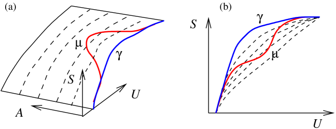
Figure 2: (a) Entropy $S$ as a function of $(U,A)$. The $\mu$ trajectory on the surface represents a microcanonical path, whereas the $\gamma$ trajectory represents a canonical path. The dashed lines represents curves with constant $A$. (b) Projection on the $(S,U)$ plane.

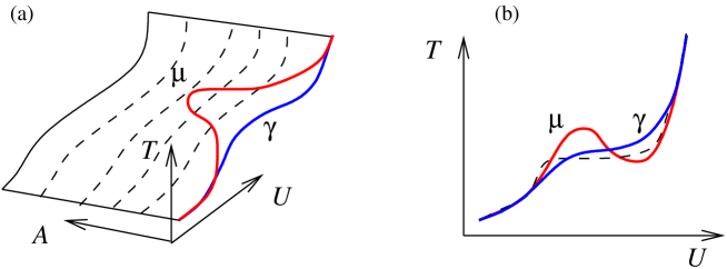
Figure 3: (a) Temperature $T$ as a function of $(U,A)$. The $\mu$ trajectory on the surface represents a microcanonical path, whereas the $\gamma$ trajectory represents a canonical path. The dashed lines represents curves with constant $A$. (b) Projection on the $(T,U)$ plane.

3 Surface of tension

In the interval of energies where $\partial U/\partial T$ is negative, such as that given by microcanonical calculations, there is a loop in the curve of temperature versus energy. In the thermodynamic limit the loop gives away and is replaced by a tie line, a straight line segment along which the temperature is constant, indicating the coexistence of thermodynamic phases. It is natural to presume that the system in this situation is not homogeneous, exhibiting coexisting heterogeneous regions with an interface of tension between them [17, 18]. In accordance with this point of view, the increase in energy of a system is equal to the heat introduced plus the the work performed by the surface tension. In differential form [19],

$$dU=TdS+\sigma dA,$$ (11)

where $\sigma$ is the surface tension and $A$ is the area of the interface. Eq. (11) describes the Gibbs equilibrium surface shown in Fig. 2a, which holds the property of convexity.

Within the microcanonical ensemble, the energy $U$ and other extensible variables are kept constant, and, according to Eq. (10), the heat capacity would coincide with the variation of the energy with temperature. However, the system described by the microcanonical ensemble might develop internal structures, characterized by extensible variables that are not or could not be kept constant. An example of this structure is the interface between two coexisting thermodynamic phases, characterized by its area. Therefore, the variation of energy with temperature may not coincide with the heat capacity because the area of the interface, which is an extensible variable, is not constant and we could not use Eq. (10).

In the microcanonical ensemble, the entropy $S$ is determined from partition function $\Omega$ through the Boltzmann formula $S=k_{B}\ln\Omega$, and the area $A$ of the interface could also be determined. As one increases the energy $U$ from small values, $S$ and $A$ will vary, and a trajectory is traced on the Gibbs surface as shown in Fig. 2a, which we call a trajectory $\mu$. The projection of the trajectory $\mu$ on the plane $(S,U)$ may lack the convexity property as seen in Fig. 2b.

From the entropy $S$, and in accordance with Eq. (11), the temperature is determined by

$$T=\left(\frac{\partial U}{\partial S}\right)_{A},$$ (12)

and, knowing $U$ and $A$, we may draw the trajectory $\mu$ shown in Fig. 3a. The projection of the trajectory $\mu$ in the plane $(T,U)$ may not be monotonic as seen in Fig. 3b. This explain the negative value of $\partial U/\partial T$ observed in the microcanonical calculations, but this quantity is not the heat capacity. In actual microcanonical numerical simulations, the temperature is not determined by Eq. (12), which would be unpractical, but by alternative schemes which may or may not coincide with formula (12). For instance, in simulations of classical systems of interacting particles it is usual to determine the temperature by assuming that it is proportional to the average of the kinetic energy.

Along the microcanonical trajectory $\mu$, the heat capacity $C_{\mu}=T(\partial S/\partial T)_{\mu}$ is not equal to $(\partial U/\partial T)_{\mu}$, in general. Indeed, from Eq. (11),

$$\left(\frac{\partial U}{\partial T}\right)_{\mu}=C_{\mu}+\sigma\left(\frac{\partial A}{\partial T}\right)_{\mu},$$ (13)

and $(\partial U/\partial T)_{\mu}$ is not the heat capacity and may be negative if $(\partial A/\partial T)_{\mu}$ is negative. If we define $\lambda=(\partial A/\partial U)_{\mu}$, which measures the change of the area with the energy along the trajectory $\mu$, it follows from (13) that

$$\left(\frac{\partial T}{\partial U}\right)_{\mu}=\frac{1-\sigma\lambda}{C_{\mu}}.$$ (14)

As one increases the energy starting from small values, the area $A$ of the interface begins to increase from zero, reaches a maximum, and then decreases and vanishes again. At the beginning, $\lambda$ is positive, then vanishes, and then becomes negative. In the interval where $\lambda$ is positive, if it is large enough, the quantity $(\partial T/\partial U)_{\mu}$, which is the slope of the microcanonical curve of Fig. 3b, will be negative.

In the canonical ensemble, the temperature $T$, which is a parameter, and the extensible variables other than energy are kept constant. As one varies the parameter $T$, a trajectory is traced on the surfaces shown in Figs. 2a and 3a, which we call a trajectory $\gamma$. The entropy is determined by the Gibbs expression

$$S=-k_{B}\int P\ln Pdxdp,$$ (15)

where $P$ is the probability density defined on the phase space $(x,p)$ and the energy $U$ is the average of the energy function.

The following relation exists between the entropy and the energy, $S=(U/T)+k_{B}\ln Z$, where $Z$ is the canonical partition function. From this relation we get

$$\left(\frac{\partial U}{\partial T}\right)_{\gamma}=T\left(\frac{\partial S}{\partial T}\right)_{\gamma},$$ (16)

and we may conclude by comparison with the relation analogous to (13) that $(\partial A/\partial T)_{\gamma}=0$ in the canonical ensemble, justifying the constance of $A$ in the trajectory $\gamma$, shown in Figs. 2a and 3a.

The right-hand side of Eq. (16) is the heat capacity $C_{\gamma}$ along the canonical trajectory and in this case

$$C_{\gamma}=\left(\frac{\partial U}{\partial T}\right)_{\gamma},$$ (17)

that is, the heat capacity is identified with the slope of $U$ versus $T$. Within the canonical ensemble, $(\partial U/\partial T)_{\gamma}$ is proportional to the variance of the energy function and $C_{\gamma}$ is a nonnegative quantity as demanded by the property of convexity of the Gibbs surface.

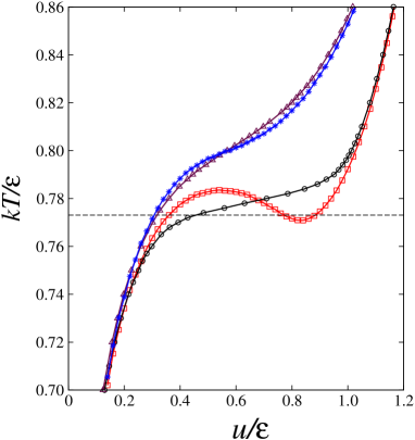
Figure 4: Temperature $T$ as a function of the energy per site $u$ for the seven-state Potts model on a square lattice with $N=400$ sites, obtained from the canonical (circles and triangles) and microcanonical (squares and stars) ensembles. The horizontal dashed line represents the temperature of coexistence in the thermodynamic limit, $T_{0}=0.773058$. The two curves (circles and squares) were obtained with periodic boundary conditions. The other two curves (triangles and stars) were obtained with fixed boundary conditions.

4 Potts model

The Potts model [20] is defined on a regular lattice in which each site can be in one of $q$ states. The interaction between two nearest neighbor sites is $\varepsilon>0$ if the sites are in different states and zero if they are in the same state. In two dimensions it is known that a phase transition takes place at the temperature $k_{B}T/\varepsilon=1/\ln(1+\sqrt{q})$, which is discontinuous if $q>4$. This is the case of the seven-state model on a square lattice, which we focus here.

In the canonical simulations, in which $T$ is a fixed parameter, we have employed the standard Metropolis algorithm and determined the energy $U$ as the average of the energy function. In the microcanonical simulations, we used transition rules that keep the energy function strictly constant. At each time step of the simulation, two sites of the lattice are chose at random and trial states chosen at random are assigned to the sites. If the energy remains the same, the trial states become the new states of the two sites. The temperature is not obtained by formula (12), which would be unpractical, but by a procedure that assumes a local canonical distribution as follows [21, 22]. Let us consider a configuration of the lattice and look for all sites whose neighboring sites are in the same state. Among the sites of this type, we distinguish those which are in the same state as its neighbors, and those which are in a state distinct form its neighbors. We denonte by $n_{0}$ the number of site of the former type and by $n_{1}$ that of the later type. If we use the canonical ensemble it is straightforward to show that the ratio of their averages is is given by

$$\frac{\langle n_{0}\rangle}{\langle n_{1}\rangle}=e^{-4\varepsilon/k_{B}T}.$$ (18)

This formula is then used in microcanonical ensemble to calculate the temperature by considering that the averages are determined from the microcanonical simulations.

Fig. 4 shows the temperature versus the energy for the standard seven-state Potts model on a finite square lattice, which we have obtained by Monte Carlo simulations by using the microcanonical and canonical ensembles, and two types of boundary conditions. One of them is the periodic boundary conditions. In the other type, which we call fixed boundary conditions, all sites at the boundary remains permanently in one of the seven states. When we use the microcanonical ensemble and periodic boundary conditions, there is an interval in the energy for which $\partial U/\partial T$ is indeed negative, as can be seen in Fig. 4. Notice that, this does not happen for the microcanonical ensemble and fixed boundary conditions, and for the canonical ensemble for both conditions. In all these three cases, the temperature is a monotonic increasing function of the energy, as seen in Fig. 4.

The loop observed in the curve of Fig. 4 disappears in the thermodynamic limit giving raise to a tie line. Assuming that the area of the interface scales like $N^{\alpha}$, with $\alpha<1$, the quantity $\lambda$ in Eq. (14) scales like $N^{\alpha-1}$ and vanishes in the thermodynamic limit, and $(\partial T/\partial u)_{\mu}$ approaches $1/c_{\mu}$ where $c_{\mu}=C_{\mu}/N$ is the specific heat. In fact, for values of $u$ within the tie line, both quantities approach the zero value. The deviation of $T$ from $T_{0}$ also scales like $N^{\alpha-1}$. The exponent $\alpha$ is expected to be equal to $(d-1)/d$ which in two dimension gives $\alpha=1/2$ [14, 17].

5 Conclusion

We have analyzed the positivity of the heat capacity and emphasized this property as the condition for stability of thermodynamic systems. We have shown that the slope of the curves of energy versus temperature may not coincide with the heat capacity. This is the case of the calculations performed within the microcanonical ensemble with periodic boundary conditions. This point is understood if we consider a microcanonical trajectory on the Gibbs equilibrium surface. This surface of the thermodynamic space spanned by the extensible variables has the convexity property. However, the projection of a trajectory on the entropy-energy plane might lack convexity. Analogously, the equation of state surface has the property of monotonicity but the projection of a trajectory on the temperature-energy plane might lack this property. The absence of monotonicity, which is manifest by the negative slope is not in contradiction with the positivity of the heat capacity because $\partial U/\partial T$ is not the heat capacity.

References

- [1] T. Tomé and M. J. de Oliveira, Phys. Rev. E 91, 042140 (2015).
- [2] L. D. Landau and E. M. Lilfshitz, Statistical Physics (Pergamon Press, London, 1958).
- [3] M. J. de Oliveira, Equilibrium Thermodynamics (Springer, 2015).
- [4] P. Hertel and W. Thirring, Ann. Phys. 63, 520 (1971).
- [5] D. H. E. Gross, A. Ecker, and X. Z. Zhang, Ann. Physik 5, 446 (1996).
- [6] I. Ispolatov and E. G. D. Cohen, Physica 295, 475 (2001).
- [7] D. H. E. Gross, Microcanonical Thermodynamics: Phase Transitions in Finite Systems (World Scientific, Singapore, 2001).
- [8] T. Dauxois, S. Ruffo, E. Arimondo, and M. Wilkens (eds.), Dynamics and Thermodynamics of Systems with Long-Range Interactions, (Springer, Berlin, 2002).
- [9] W. Thirring, H. Narnhofer, and H. A. Posch, Phys. Rev. Lett. 91, 130601 (2003).
- [10] D. H. E. Gross, J. Chem. Phys. 122, 224111 (2005).
- [11] H. Behringer and M. Pleimling, Phys. Rev. E 74, 011108 (2006).
- [12] J. Dunkel and S. Hilbert, Physica A 370, 390 (2006).
- [13] V. Martin-Mayor, Phys. Rev. Lett. 98, 137207 (2007).
- [14] C. E. Fiore and M. J. de Oliveira, Computer Physics Communications 80, 1434 (2009).
- [15] M. A. Carignano and I. Gladich, Europhysics Letters 90, 63001 (2010).
- [16] S. Schnabel, D. T. Seaton, D. P. Landau, and M. Bachmann, Phys. Rev. E 84, 011127 (2011).
- [17] A. Tröster and K. Binder, J. Phys.: Condens. Matter 24, 284107 (2012).
- [18] H.-J. Zhou, Phys. Rev. Lett. 122 160601 (2019).
- [19] J. S. Rowlinson and B. Widom, Molecular Theory of Capillarity (Clarendon Press, Oxford, 1982).
- [20] F. Y. Wu, Rev. Mod. Phys. 54, 235 (1982).
- [21] C. S. Shida, V. B. Henriques, and M. J. de Oliveira, Phys. Rev. E 68, 066125 (2003).
- [22] C. E. Fiore, V. B. Hneriques, and M. J. de Oliveira, J. Chem. Phys. 125, 164509 (2006)