Considering Likelihood in NLP Classification Explanations with Occlusion and Language Modeling

Abstract

Recently, state-of-the-art NLP models gained an increasing syntactic and semantic understanding of language, and explanation methods are crucial to understand their decisions. Occlusion is a well established method that provides explanations on discrete language data, e.g. by removing a language unit from an input and measuring the impact on a model’s decision. We argue that current occlusion-based methods often produce invalid or syntactically incorrect language data, neglecting the improved abilities of recent NLP models. Furthermore, gradient-based explanation methods disregard the discrete distribution of data in NLP. Thus, we propose OLM: a novel explanation method that combines occlusion and language models to sample valid and syntactically correct replacements with high likelihood, given the context of the original input. We lay out a theoretical foundation that alleviates these weaknesses of other explanation methods in NLP and provide results that underline the importance of considering data likelihood in occlusion-based explanation.

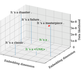
Figure 1: Schematic display of data likelihood in NLP. There are discrete inputs, i.e. combination of tokens, with a data likelihood greater than zero. All other inputs in the embedding space have likelihood zero because they have no corresponding tokens. Occlusion methods (green) create unlikely input. Gradient-based explanation methods (red arrow) consider infinitesimal changes to the input and thus data with no likelihood.

Method	Relevances	Max. value
OLM (ours)	forced , familiar and thoroughly condescending .	0.76
OLM-S (ours)	forced , familiar and thoroughly condescending .	0.47
Delete	forced , familiar and thoroughly condescending .	1
UNK	forced , familiar and thoroughly condescending .	0.35
Sensitivity Analysis	forced , familiar and thoroughly condescending .	0.025
Gradient*Input	forced , familiar and thoroughly condescending .	0.00011
Integrated Gradients	forced , familiar and thoroughly condescending .	0.68

Table 1: Relevance scores of different gradient- and occlusion-based explanation methods for a sentence from the SST-2 dataset, correctly classified as negative sentiment by RoBERTa. Red indicates an input token, with a contribution to the true label (negative sentiment), blue indicates a detraction from the true label. Coloring are normalized for each method for visibility, the maximum value of each method is indicated in the last column. The relevances of the first four and last method can be interpreted as prediction difference if that token is missing (see Sensitivity-1 in 2.1). The first token “forced” only has high relevance for our methods, the most commonly resampled tokens can be found in Table 2. Punctuation marks have less relevance than words for our method compared to gradient methods.

1 Introduction

Explanation methods are a useful tool to analyze and understand the decisions made by complex non-linear models, e.g. neural networks. For example, they can attribute relevance scores to input features (e.g. word or sub-word units in NLP). Gradient-based methods provide explanations by analyzing local infinitesimal changes to determine the shape of a network’s function. The implicit assumption is that the local shape of a function is indicative or useful to calculate the relevance of an input feature for a model’s prediction. In computer vision, for example, infinitesimal changes to an input image still produce another valid image and the change in prediction is a valid tool to analyze what led to it (e.g., Zintgraf et al., 2017). The same applies to methods that analyze the function’s gradient at multiple points, such as Integrated Gradients Sundararajan et al. (2017).

In NLP, however, the input consists of natural language, which is discrete, i.e., the data that has positive likelihood is a discrete distribution (see Figure 1). This means that local neighborhoods need not be indicative of the model’s prediction behaviour and a model’s prediction function at points with zero likelihood need not be relevant to the model’s decision. Thus, we argue that black-box models in NLP should be analyzed only at inputs of non-zero likelihood and explanation methods should not rely on gradients. Occlusion is a well suited method due to its ability to produce explanations on data with discrete likelihood. For example, by replacing or deleting a language unit in the original input and measuring the impact on the model’s prediction. However, the likelihood of the replacement data is usually low. Consider, for example, a sentiment classification task and assume a model that assigns syntactically incorrect inputs a negative sentiment. It correctly predicts “It ’s a masterpiece .” as positive, but assigns negative sentiment to syntactically incorrect inputs produced by occlusion, e.g. “It ’s a .” or “It ’s a $<$UNK$>$ .”, which have low data likelihood (see Figure 1). This may result in a large prediction difference for many tokens in a positive sentiment example and no prediction difference for many tokens in a negative sentiment example (see Table 1), independent of whether they carry any sentiment information and thus may be relevant to the model. This example shows that the relevance attributed by current occlusion-based methods may depend solely on the model’s syntactic understanding instead of the input feature’s information regarding the task.

We argue that current NLP state-of-the-art models have increasing syntactic (Hewitt and Manning, 2019) and hierarchical (Liu et al., 2019a) understanding. Therefore, methods that explain these models should consider syntactically correct replacement that is likely given the unit’s context, e.g. in Figure 1 “classic” or “failure” as replacements for “masterpiece” in “It ’s a masterpiece .” Our experiments show that presenting these models with perturbed ungrammatical input changes the explanations.

1.1 Contributions

• We present OLM, a novel black-box relevance explanation method which considers syntactic understanding. It is suitable for any model that performs an NLP classification task and we analyze which axioms for explanation methods it fulfills.

• We introduce the class zero-sum axiom for explanation methods.

• We experimentally compare the relevances produced by our method to those of other black-box and gradient-based explanation approaches.

2 Methods

In this section, we introduce our novel explanation method that combines occlusion with language modeling. Instead of deleting or replacing a linguistic unit in the input with an unlikely replacement, OLM substitutes it with one generated by a language model. This produces a contextualized distribution of valid and syntactically likely reference inputs and allows a more faithful analysis of models with increasing syntactic capabilities. This is followed by an axiomatic analysis of OLM’s properties. Finally, we introduce OLM-S, an extension that measures sensitivity of a model at a feature’s position.

For our approach we employ the difference of probabilities formula from Robnik-Šikonja and Kononenko (2008). Let $x_{i}$ be an attribute of input $x$ and $x_{\setminus i}$ the incomplete input without this attribute. Then the relevance $r$ given the prediction function $f$ and class $c$ is

$$r_{f,c}(x_{i})=f_{c}(x)-f_{c}(x_{\setminus i}).$$ (1)

Note that $f_{c}(x_{\setminus i})$ is not accurately defined and needs to be approximated, as $x_{\setminus i}$ is an incomplete input. For vision, Zintgraf et al. (2017) approximate $f_{c}(x_{\setminus i})$ by using the input data distribution $p_{data}$ to sample $\hat{x}_{i}$ independently of $x$ or use a Gaussian distribution for $\hat{x}_{i}$ conditioned on surrounding pixels. We argue sampling should be conditioned on the whole input and depend on the probability of the data distribution. We argue that in NLP a language model $p_{LM}$ generates input that is as natural as possible for the model and thus approximate

$$f_{c}(x_{\setminus i})\approx\sum_{\hat{x}_{i}}p_{LM}(\hat{x}_{i}|x_{\setminus i})f_{c}(x_{\setminus i},\hat{x}_{i}).$$ (2)

In general, $x_{i}$ should be units of interest such as phrases, words or subword tokens. Thus, OLM’s relevance for a language unit is the difference in prediction between the original input and inputs with the unit resampled by conditioning on information in its context. The relevance of every language unit is in the interval $[-1,1]$, with the sign indicating contradiction or support, and can be interpreted as the value of information added by the unit for the model.

token	freq.	pred.	token	freq.	pred.
familiar	9	1	old	2	1
warm	4	7e-4	perfect	2	3.9e-4
ancient	3	0.074	quiet	2	1
cold	3	1	real	2	6.5e-3
beautiful	2	1.4e-4	sweet	2	1.9e-4
bold	2	0.63	wonderful	2	3.1e-4
low	2	1	yes	2	1
nice	2	8.3e-4	young	2	0.99

Table 2: Most frequently resampled words for “forced” in “forced , familiar and thoroughly condescending .” from Table 1 with the prediction of the true label neuron (negative sentiment). We sample 100 times per token, the prediction is rounded to two significant digits. Many resampled words lead to a positive sentiment classification. The high variance of the model prediction for replacements of this token is not captured by another method.

2.1 Axiomatic Analysis

Sundararajan et al. (2017) introduced axiomatic development and analysis of explanation methods. We follow their argument that an explanation method should be derived theoretically, not experimentally, as we want to analyze a model, not our understanding of it. First, we introduce a new axiom. Then we discuss which existing axioms our method fulfills.

Class Zero-Sum Axiom. We introduce an axiom that follows from the intuition that for a normalized DNN every input feature contributes as much to a specific class as it detracts from all other classes. Let $f$ be a prediction function where the output is normalized over all classes $C$. Every input feature contributes as much to the classification of a specific class as it detracts from other classes. A relevance method that gives a feature positive relevance for every class is not helpful in understanding the model. An explanation method satisfies Class Zero-Sum if the summed relevance of each input feature $x_{i}$ over all classes is zero.

$$\sum_{c\in C}r_{f,c}(x_{i})=0$$ (3)

This axiom can be seen as an alternative to the Completeness axiom given by Bach et al. (2015). Completeness states that the sum of the relevances of an input is equal to its prediction. They can not be fulfilled simultaneously. Gosiewska and Biecek (2019) show that a linear distribution of relevance as with Completeness is not necessarily desirable for non-linear models. They argue that explanations that force the sum of relevances to be equal to the prediction do not capture the interaction of features faithfully. OLM fulfills Class Zero-Sum, as do other occlusion methods and gradient methods. Other axioms OLM fulfills are:

Implementation Invariance. Two neural networks that represent the same function, i.e. give the same output for each possible input, should receive the same relevances for every input (Sundararajan et al., 2017).

Linearity. A network, which is a linear combination of other networks, should have explanations which are the same linear combination of the original networks explanations (Sundararajan et al., 2017).

Sensitivity-1. The relevance of an input variable should be the difference of prediction when the input variable is occluded (Ancona et al., 2018).

	MNLI		SST-2		CoLA
	OLM	OLM-S	OLM	OLM-S	OLM	OLM-S
Delete	0.60	-	0.52	-	0.25	-
UNK	0.58	-	0.47	-	0.21	-
Sensitivity Analysis	0.27	0.35	0.30	0.37	0.20	0.29
Gradient*Input	-0.03	-	0.02	-	0.02	-
Integrated Gradients	0.28	-	0.35	-	0.15	-

Table 3: Correlation between explanation methods on MNLI, SST-2, and CoLA development sets. OLM correlates with every method except for Gradient*Input. The correlation is highest with the other Occlusion methods for MNLI and SST-2 but not close to 1. For all methods, the correlation is lowest on CoLA.

2.2 OLM-S

From our approach we can also deduce a method that describes the sensitivity of the classification at the position of an input feature. To this end, we compute the standard deviation of the language model predictions.

$$s_{f,c}(x_{i})=\sqrt{\sum_{\hat{x}_{i}}p_{LM}(\hat{x}_{i}|x_{\setminus i})\left(f_{c}(x_{\setminus i},\hat{x}_{i})-\mu\right)^{2}},$$ (4)

where $\mu$ is the mean value from equation 2. We call this OLM-S(ensitivity). Note that this measure is independent of $x_{i}$ and only describes the sensitivity of the feature’s position. This means that it measures a model’s sensitivity at a given language unit’s position given the context. OLM and OLM-S are thus using mean and standard deviation, respectively, of the prediction when resampling a token.

3 Experiments

In our experiments, we aim to answer the following question: Do relevances produced by our method differ from those that either ignore the discrete structure of language data or produce syntactically incorrect input, and if so, how?

We first train a state-of-the-art NLP model (RoBERTa, Liu et al., 2019b) on three sentence classification tasks (Section 3.2). We then compare the explanations produced by OLM and OLM-S to five occlusion and gradient-based methods (Section 3.1). To this end, we calculate the relevances of words over a whole input regarding the true label. We calculate the Pearson correlation coefficients of these relevances for every sentence and average this over the whole development set of each task. In our experiments we use BERT base (Devlin et al., 2019) for OLM resampling.

3.1 Baseline Methods

We compare OLM with occlusion (Robnik-Šikonja and Kononenko, 2008; Zintgraf et al., 2017) in two variants. One method of occlusion is deletion of the word. The other method is replacing the word with the $<$UNK$>$ token for unknown words. These methods can produce ungrammatical input, as we argue in Section 1.

Furthermore, we compare with the following gradient-based methods. Sensitivity Analysis (Simonyan et al., 2013) is the absolute value of the gradient. Gradient*Input (Shrikumar et al., 2016) is simple component-wise multiplication of an input with its gradient. Integrated Gradients (Sundararajan et al., 2017) integrate the gradients from a reference input to the current input. As these gradient-based methods provide relevance for every word vector value, we sum up all vector values belonging to a word. Gradient-based methods do not consider likelihood in NLP (see Section 1) and are thus also merely a comparison and not a gold standard.

3.2 Tasks

We select a representative set of NLP sentence classification tasks that focus on different aspects of context and linguistic properties:

MNLI (matched) The Multi-Genre Natural Language Inference Corpus Williams et al. (2018) contains 400k pairs of premise and hypothesis sentences and the task is to predict whether the premise entails the hypothesis. We re-use the RoBERTa large model fine-tuned on MNLI Liu et al. (2019b), with a dev set accuracy of 90.2.

SST-2 The Stanford Sentiment Treebank Socher et al. (2013) contains 70k sentences labeled with positive or negative sentiment. We fine-tune the pre-trained RoBERTa base to the classification task and achieve an accuracy of 94.5 on the dev set.

CoLA The Corpus of Linguistic Acceptability Warstadt et al. (2018) contains 10k sentences labeled as grammatical or ungrammatical, e.g. ‘They can sing.’ (acceptable) vs.  ‘many evidence was provided.’ (unacceptable). Similar to SST-2, we fine-tune RoBERTa base to the task and achieve a Matthew’s corr.  of 61.3 on the dev set.

3.3 Results

Table 3 shows the correlation of our two proposed occlusion methods (OLM and OLM-S) with other explanation methods on three NLP tasks. For OLM-S we only report correlation to Sensitivity because both inform about the magnitude of possible change. They both provide non-negative values and therefore are not necessarily comparable to the other methods. We find that across all tasks OLM correlates the most with the two occlusion-based methods (Unk and Delete) but the overall correlation is low, with a maximum of 0.6 on MNLI. Also the level differs greatly between tasks, ranging from 0.21 and 0.25 (Unk, Delete) on CoLA to 0.58 and 0.6 on MNLI. As this is an average of correlations, this shows that resampling creates distinctive explanations that can not be approximated by other occlusion methods. An example input from SST-2 can be found in Table 1, which clearly highlights the difference in explanations. Table 2 shows the corresponding tokens resampled by OLM, using BERT base as the language model. For gradient-based methods the correlation with OLM is even lower, ranging from -0.03 for Gradient*Input on MNLI to 0.35 for Integrated Gradients on SST-2. For OLM-S we observe a correlation between 0.29 (CoLA) and 0.35 (MNLI), which is still low. Gradient*Input shows almost no correlation to OLM across tasks. The overall low correlation of gradient-based methods with OLM and OLM-S suggests that ignoring the discrete structure of language data might be problematic in NLP.

4 Related Work

There exist many other popular black-box explanation methods for DNNs. SHAP (Lundberg and Lee, 2017) is a framework that uses Shapley Values which are a game-theoretic black-box approach to determining relevance by occluding subsets of all features. They do not necessarily consider the likelihood of data. The occlusion SHAP employs may be combined with OLM but the approximation error of the language model could increase with more features occluded. LIME (Ribeiro et al., 2016) explains by learning a local explainable model. LIME tries to be locally faithful to a model, which is, as we argue, not as important as likely data for explanations in NLP.

There are also explanation methods for DNNs which give layer-specific rules to retrieve relevance. LRP (Bach et al., 2015) propagates relevance from the output to the input such that Completeness is satisfied for every layer. DeepLIFT (Shrikumar et al., 2017) compares the activations of an input with activations reference inputs. In contrast to OLM, these layer-specific explanation methods have been shown not to satisfy Implementation Invariance Sundararajan et al. (2017).

Most state-of-the-art models in NLP are transformers which use attention. There is a discussion on whether attention weights (Bahdanau et al., 2015; Vaswani et al., 2017) should be considered as explanation method in Jain and Wallace (2019) and Wiegreffe and Pinter (2019). They are not based on an axiomatic attribution of relevances. It is unclear whether they satisfy any axiom. An advantage to analyzing attention weights is that attention weights naturally show what the model does. Thus, even if they do not always provide a faithful explanation, their analysis might be helpful for a specific input.

5 Conclusion

We argue that current black-box and gradient-based explanation methods do not yet consider the likelihood of data and present OLM, a novel explanation method, which uses a language model to resample occluded words. It is especially suited for word-level relevance of sentence classification with state-of-the-art NLP models. We also introduce the Class Zero-Sum Axiom for explanation methods, compare it with an existing axiom. Furthermore, we show other axioms that OLM satisfies. We argue that with this more solid theoretical foundation OLM can be regarded as an improvement over existing NLP classification explanation methods. In our experiments, we compare our methods to other occlusion and gradient explanation methods. We do not consider these experiments to be exhaustive. Unfortunately, there is no general evaluation for explanation methods.

We show that our method adds value by showing distinctive results and better founded theory. A practical difficulty of OLM is the approximation with a language model. First, a language model can create syntactically correct data, that does not make sense for the task. Second, even state-of-the-art language models do not always produce syntactically correct data. However, we argue that using a language model is a suitable way for finding reference inputs.

In the future, we want to extend this method to language features other than words. NLP tasks with longer input are probably not very sensitive to single word occlusion, which could be measured with OLM-S.

Appendix A Proof Appendix

Let $f$ be a neural network that predicts a probability distribution over classes $C$, i.e. $\sum_{c\in C}f_{c}(x)=1$. Let $x=(x_{1},...,x_{n})$ be a input split into $n$ input features.

1. Class Zero-Sum and Completeness rule each other out. Assume $r_{f,c}$ fulfills both, then we have

$$\sum_{i=1}^{n}\sum_{c\in C}r_{f,c}(x_{i})=0$$ (5)

from Class Zero-Sum and

$$\sum_{c\in C}\sum_{i=1}^{n}r_{f,c}(x_{i})=1$$ (6)

from Completeness. Contradiction.

2. OLM satisfies Class Zero-Sum. Let $r_{f,c}$ now be the OLM relevance method from equations (1) and (2) in the paper.

$$\begin{split}&\sum_{c\in C}r_{f,c}(x_{i})\\ =&\sum_{c\in C}\left(f_{c}(x)-\sum_{\hat{x}_{i}}p_{LM}(\hat{x}_{i}|x_{\setminus i})f_{c}(x_{\setminus i},\hat{x}_{i})\right)\\ =&\sum_{c\in C}f_{c}(x)-\sum_{\hat{x}_{i}}p_{LM}(\hat{x}_{i}|x_{\setminus i})\sum_{c\in C}f_{c}(x_{\setminus i},\hat{x}_{i})\\ =&1-\sum_{\hat{x}_{i}}p_{LM}(\hat{x}_{i}|x_{\setminus i})=0.\end{split}$$ (7)

3. OLM satisfies Implementation Invariance. OLM is a black box method and only evaluates the function of the neural network. Thus, it has to satisfy Implementation Invariance.

4. OLM satisfies Sensitivity-1. OLM is defined as an Occlusion method, so it necessarily gives the difference of prediction when an input variable is occluded.

5. OLM satisfies Linearity. Let $f=\sum_{j=1}^{n}\alpha_{j}g^{j}$ be a linear combination of models. Then we have

$$\begin{split}r_{f,c}(x_{i})=&f_{c}(x)-\sum_{\hat{x}_{i}}p_{LM}(\hat{x}_{i}|x_{\setminus i})f_{c}(x_{\setminus i},\hat{x}_{i})\\ =&\sum_{j=1}^{n}\alpha_{j}g_{c}^{j}(x)-\\ &\quad\sum_{\hat{x}_{i}}p_{LM}(\hat{x}_{i}|x_{\setminus i})\sum_{j=1}^{n}\alpha_{j}g_{c}^{j}(x_{\setminus i},\hat{x}_{i})\\ =&\sum_{j=1}^{n}\alpha_{j}r_{g^{j},c}(x_{i}).\end{split}$$ (8)

References

- Ancona et al. (2018) Marco Ancona, Enea Ceolini, Cengiz Öztireli, and Markus Gross. 2018. Towards better understanding of gradient-based attribution methods for deep neural networks. International Conference on Learning Representations.
- Bach et al. (2015) Sebastian Bach, Alexander Binder, Grégoire Montavon, Frederick Klauschen, Klaus-Robert Müller, and Wojciech Samek. 2015. On pixel-wise explanations for non-linear classifier decisions by layer-wise relevance propagation. PloS one, 10(7):e0130140.
- Bahdanau et al. (2015) Dzmitry Bahdanau, Kyunghyun Cho, and Yoshua Bengio. 2015. Neural machine translation by jointly learning to align and translate. International Conference on Learning Representations.
- Devlin et al. (2019) Jacob Devlin, Ming-Wei Chang, Kenton Lee, and Kristina Toutanova. 2019. BERT: Pre-training of deep bidirectional transformers for language understanding. In Proceedings of the 2019 Conference of the North American Chapter of the Association for Computational Linguistics: Human Language Technologies, Volume 1 (Long and Short Papers), pages 4171–4186. Association for Computational Linguistics.
- Gosiewska and Biecek (2019) Alicja Gosiewska and Przemyslaw Biecek. 2019. Do not trust additive explanations. CoRR, arXiv:1903.11420.
- Hewitt and Manning (2019) John Hewitt and Christopher D. Manning. 2019. A structural probe for finding syntax in word representations. In Proceedings of the 2019 Conference of the North American Chapter of the Association for Computational Linguistics: Human Language Technologies, Volume 1 (Long and Short Papers), pages 4129–4138.
- Jain and Wallace (2019) Sarthak Jain and Byron C. Wallace. 2019. Attention is not Explanation. In Proceedings of the 2019 Conference of the North American Chapter of the Association for Computational Linguistics: Human Language Technologies, Volume 1 (Long and Short Papers), pages 3543–3556.
- Liu et al. (2019a) Nelson F. Liu, Matt Gardner, Yonatan Belinkov, Matthew E. Peters, and Noah A. Smith. 2019a. Linguistic knowledge and transferability of contextual representations. In Proceedings of the 2019 Conference of the North American Chapter of the Association for Computational Linguistics: Human Language Technologies, Volume 1 (Long and Short Papers), pages 1073–1094.
- Liu et al. (2019b) Yinhan Liu, Myle Ott, Naman Goyal, Jingfei Du, Mandar Joshi, Danqi Chen, Omer Levy, Mike Lewis, Luke Zettlemoyer, and Veselin Stoyanov. 2019b. Roberta: A robustly optimized BERT pretraining approach. CoRR, arXiv:1907.11692.
- Lundberg and Lee (2017) Scott M. Lundberg and Su-In Lee. 2017. A unified approach to interpreting model predictions. In I. Guyon, U. V. Luxburg, S. Bengio, H. Wallach, R. Fergus, S. Vishwanathan, and R. Garnett, editors, Advances in Neural Information Processing Systems 30, pages 4765–4774. Curran Associates, Inc.
- Ribeiro et al. (2016) Marco Tulio Ribeiro, Sameer Singh, and Carlos Guestrin. 2016. Why should i trust you?: Explaining the predictions of any classifier. In Proceedings of the 22nd ACM SIGKDD international conference on knowledge discovery and data mining, pages 1135–1144. ACM.
- Robnik-Šikonja and Kononenko (2008) Marko Robnik-Šikonja and Igor Kononenko. 2008. Explaining classifications for individual instances. IEEE Transactions on Knowledge and Data Engineering, 20(5):589–600.
- Shrikumar et al. (2017) Avanti Shrikumar, Peyton Greenside, and Anshul Kundaje. 2017. Learning important features through propagating activation differences. In International Conference on Machine Learning, pages 3145–3153.
- Shrikumar et al. (2016) Avanti Shrikumar, Peyton Greenside, Anna Shcherbina, and Anshul Kundaje. 2016. Not just a black box: Learning important features through propagating activation differences. CoRR, arXiv:1605.01713.
- Simonyan et al. (2013) Karen Simonyan, Andrea Vedaldi, and Andrew Zisserman. 2013. Deep inside convolutional networks: Visualising image classification models and saliency maps. CoRR, arXiv:1312.6034.
- Socher et al. (2013) Richard Socher, Alex Perelygin, Jean Wu, Jason Chuang, Christopher D. Manning, Andrew Ng, and Christopher Potts. 2013. Recursive deep models for semantic compositionality over a sentiment treebank. In Proceedings of EMNLP, pages 1631–1642.