Variational theory for the ground state and collective excitations of an elongated dipolar condensate
Abstract
We develop a variational theory for a dipolar condensate in an elongated (cigar shaped) confinement potential. Our formulation provides an effective one-dimensional extended meanfield theory for the ground state and its collective excitations. We apply our theory to investigate the properties of rotons in the system comparing the variational treatment to a full numerical solution. We consider the effect of quantum fluctuations on the scattering length at which the roton excitation softens to zero energy.
I Introduction
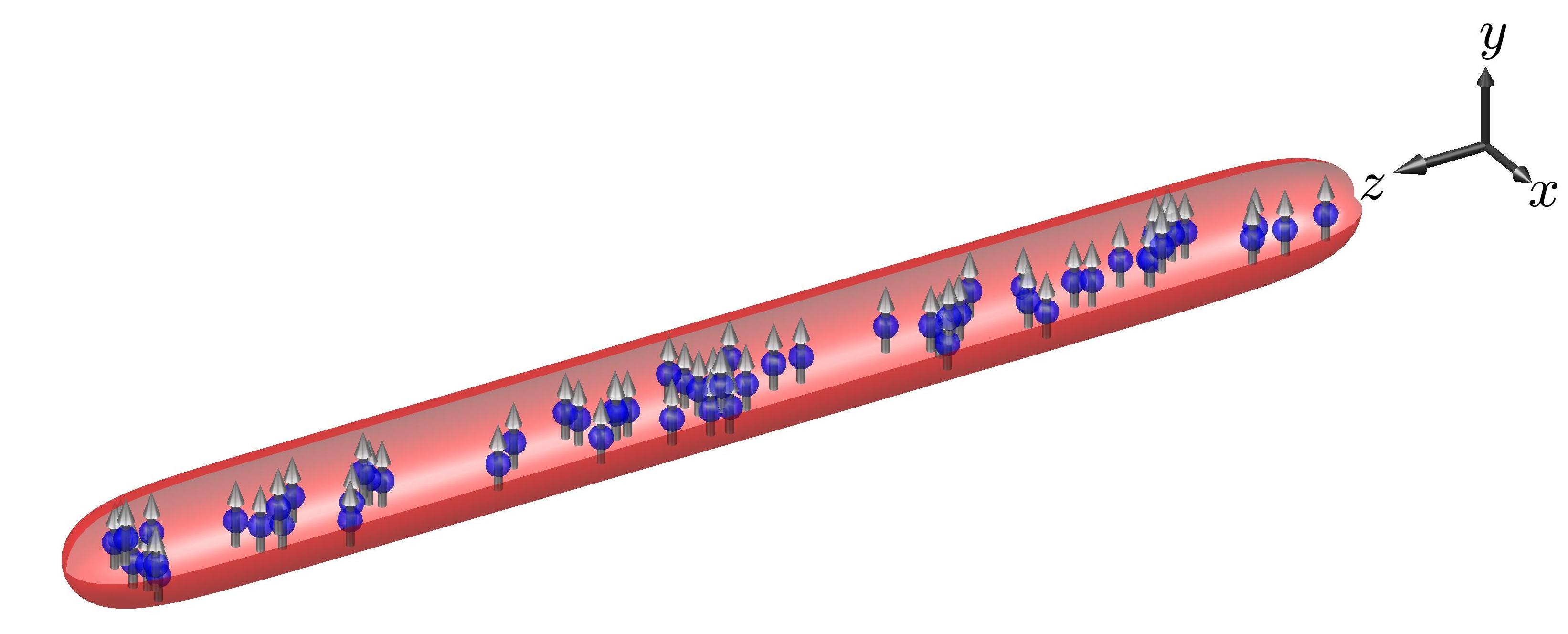
Bose-Einstein condensates (BECs) of highly magnetic atoms, such as chromium, erbium, and dysprosium Griesmaier et al. (2005); *Pasquiou2011a; Lu et al. (2011); *Lu2012a; Aikawa et al. (2012), realize a dilute quantum system with long-ranged and anisotropic dipole-dipole interactions (DDIs). Recently experiments with such dipolar condensates have observed a roton excitation Chomaz et al. (2018); Petter et al. (2019), i.e. a local minimum in the excitation dispersion relation of the condensate at a non-zero wave vector. The roton excitation, originally introduced in the study of super fluid Helium Landau (1941), has been of significant theoretical interest in dipolar condensates where it emerges from an interplay between the DDIs and confinement (e.g. see Santos et al. (2003); Ronen et al. (2007); Blakie et al. (2012); Corson et al. (2013a, b); Jona-Lasinio et al. (2013); Bisset and Blakie (2013); Baillie and Blakie (2015); Roccuzzo and Ancilotto (2019)). Much of the theoretical attention has focused on the case of a system confined to a planar (pancake) geometry with the dipoles aligned along the tightly confined direction. Experiments instead have realized roton excitations in an elongated (cigar) geometry with the dipoles oriented along one of the tightly confined directions (e.g. see Fig. 1). While the planar case can have cylindrical symmetry, the elongated system does not and in general requires a full three-dimensional (3D) calculation. Such calculations for the system ground states and its collective excitations demand significant computational resources, mostly arising from the large and dense numerical grids required to carefully resolve the singular DDI potential.
The theoretical description of a dipolar condensate is usually provided by meanfield theory. However, recent developments in the field have revealed that quantum fluctuations can play an important role in the regime of strong DDIs, for example leading to the formation of stable quantum droplets and supersolids (e.g. see Kadau et al. (2016); Ferrier-Barbut et al. (2016); Bisset et al. (2016, 2016); Chomaz et al. (2016); Schmitt et al. (2016); Böttcher et al. (2019a, b); Tanzi et al. (2019a); Chomaz et al. (2016)). Extended meanfield theory includes the leading order effects of quantum fluctuations within a local density approximation Ferrier-Barbut et al. (2016); Wächtler and Santos (2016); Bisset et al. (2016). In this formalism the stationary states of the system are described by the extended Gross-Pitaevskii equation (eGPE), with the collective excitations described by the associated Bogoliubov-de Gennes (BdG) equations Baillie et al. (2017); Lee et al. (2018).
In this paper we develop an approximation that allows us to reduce the 3D extended meanfield theory to a tractable one-dimensional (1D) form. Our approach is to use a Gaussian ansatz to describe the tightly confined transverse directions, and by integrating this out we obtain an effective 1D form of the theory, albeit with some variational parameters from the Gaussian. Such an approach is a rather obvious path to take and has been used for non-dipolar condensates (e.g. see Salasnich et al. (2002)). However, for the dipolar case the Gaussian cannot be integrated out against the DDI potential to yield an analytic result for the interaction term, except for the special case where the Gaussian is isotropic. An important result of this paper is that we introduce a useful approximate analytic result for general Gaussian. Based on this we develop a simple 1D effective theory for the stationary states and the collective excitations of the system. We emphasize that this description is for a 3D dipolar condensate, and is not applicable to the true 1D regime where interactions remain weak compared to the confinement and the quantum fluctuations take a different form Edler et al. (2017). Indeed, in the regime of interest (e.g. where rotons occur) the interaction energy scale is typically larger than the transverse confinement energy and the transverse degrees of freedom must be treated variationally. Furthermore, in this regime magnetostriction effects can be large, causing the Gaussian to distort appreciably from the geometry imposed by the confining potential. This occurs because the DDIs are anisotropic and the energy of the system is reduced by having more particles in a relative head-to-tail orientation.
We compare our results from the variational 1D theory to full numerical solutions of the 3D problem for both ground states and the excitation spectrum. We use our theory to predict the value of the s-wave scattering length (readily adjusted in experiments using Feshbach resonances) where the roton mode goes soft (i.e. to zero energy), and the associated value of the wave vector of the soft mode. By comparing to results that exclude the quantum fluctuation term we can assess the effect of quantum fluctuations on the roton properties.
II Formalism
II.1 Extended meanfield theory for dipolar condensates
II.1.1 3D Extended Gross-Pitaevskii equation (eGPE)
The system of interest is a dilute Bose gas of atoms with a magnetic moment polarized along the -axis. The extended meanfield theory for this system identifies stationary states of the matterwave field as solutions of the eGPE , where
| (1) |
Here is the chemical potential and
| (2) |
is the interaction term, with interaction potential
| (3) |
where the contact interaction coupling constant is , is the -wave scattering length, the DDI coupling constant is , and is the dipole length. This theory includes the leading order quantum fluctuations in the local density approximation, where the coefficient of this term is Lima and Pelster (2011); Wächtler and Santos (2016); Bisset et al. (2016)
| (4) |
with . The atoms are taken to be confined by an external potential . Here we focus our attention on the regime used in experiments to observe roton excitations: a cigar shaped trap with (including the pure tube case with ). The energy functional associated with the 3D eGPE is
| (5) |
II.1.2 Bogoliubov-de Gennes theory of excitations
The collective excitations of this system are Bogoliubov quasiparticles, which can be obtained by linearizing the time-dependent GPE about a stationary state as
| (6) |
where is a small complex amplitude. The quasiparticle modes and energies satisfy the BdG equations Baillie et al. (2017)
| (7) |
where is the exchange operator given by
| (8) |
II.2 Reduction to an effective 1D eGPE
II.2.1 General approach
We approximate the 3D solutions in the elongated trap to be of the separable form , where is the transverse mode function with being the radial coordinate vector and . Integrating out the transverse directions we obtain the 1D eGPE operator for the axial wavefunction :
| (9) | ||||
| (10) |
where , and
| (11) |
The effective interaction term is
| (12) |
where we have introduced the effective 1D -space interaction kernel
| (13) |
In the above results is the Fourier transform of Eq. (3), given by
| (14) |
denotes the 1D Fourier transform and denotes the 2D Fourier transform . The associated energy functional takes the form
| (15) |
II.2.2 Anisotropic Gaussian approximation
Here we introduce a convenient analytic form for . Our choice is the Gaussian
| (16) |
of mean width , and anisotropy , where () is the 1/e half width of along the -axis (-axis). We use to collectively denote the variational parameters , which are determined by minimising the system energy.
Using we can analytically evaluate key terms in the 1D theory. First we denote evaluated with as
| (17) |
Similarly, . We are unaware of a general analytic result for evaluated using , which we denote as . However, we have obtained the useful approximate result
| (18) |
with being the exponential integral111 This can also be written in terms of the incomplete Gamma function using for (cf. Ref.Sinha and Santos (2007))., and .
II.2.3 Justification for Eq. (18)
For the particular case of an isotropic Gaussian (i.e. ) Eq. (18) is exact (see Deuretzbacher et al. (2010, 2013); Giovanazzi and O’Dell (2004); Sinha and Santos (2007)). While a general analytic result for is unavailable, we can calculate the limiting behavior
| (22) |
We have arrived at result (18) by inspection and numerical experiment: it satisfies the required limiting behavior and reduces to the exact isotropic result at .
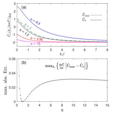
In Fig. 2 we compare the accuracy of Eq. (18) to a full calculation of the kernel obtained by numerically evaluating (13) with . To ensure the numerical calculation is accurate it is performed using a large and dense two-dimensional transverse grid of points and using a cutoff -space DDI potential to avoid finite size boundary effects (e.g. see Ronen et al. (2006)). The results in Fig. 2 show that while our approximate analytic result (18) is not identical to the numerical result, it is generally in very good agreement over a wide range of values (i.e. ). Note that ground states with can occur due to the confinement (i.e. when ), and are also favoured by the interactions when , which can be arranged by rotationally tuning the dipoles Giovanazzi et al. (2002); Tang et al. (2018). We expect that for the regimes of interest the error associated with making the Gaussian approximation is much more significant than any additional error introduced by using Eq. (18) to describe its interactions.
II.2.4 Variational theory
Here we summarise the results developed in Sec. II.2.2 and succinctly present the variational 1D eGPE theory that forms the main formalism result of this paper.
The axial orbital satisfies the 1D eGPE:
| (23) |
where
| (24) |
with , and is evaluated according to Eq. (12) but using in place of .
Since depends on we also need a procedure to obtain the parameters . To do this we consider the total system energy per particle:
| (25) |
where
| (26) | ||||
is the energy functional for the orbital, and .
For the axial wavefunction can be uniform , where is the linear density. In this regime the energy per particle (25) reduces to
| (27) |
i.e. the ground state is determined by minimising a simple nonlinear function.
II.2.5 Quasi-1D theory
Predictions for can be made within the quasi-1D approximation using the procedure outlined for the variational theory, but with and held fixed to the values for the harmonic oscillator ground state of the transverse confinement, i.e. for and , with . We denote the harmonic oscillator state as and the associated -space kernel as . This quasi-1D approximation will only be accurate when the interaction terms in remain small compared to .
II.2.6 Effective 1D form of the excitations
Making the same shape approximation for the transverse form of the excitations Baillie and Blakie (2015) we set and and integrating out the BdG equations (7) reduce to
| (28) |
where .
In general the BdG equations need to be discretised and solved numerically, however for the case of a uniform ground state an analytic solution can be obtained. Here the excitations are plane waves of momentum , i.e. , , , with excitation energy
| (29) |
where .
III Results
III.1 Numerical Methods
In this subsection we briefly outline the various numerical methods used to solve for the results we present later.
III.1.1 Uniform cases
For cases without axial trapping () we restrict our attention to the regime where the ground state is uniform and specified by the linear density .
The variational 1D eGPE theory reduces to minimising the nonlinear function (27) for and . The BdG excitation energies are then directly given by evaluating Eq. (29).
The 3D eGPE reduces to the determining the transverse mode . We do this by discretizing on a two dimensional numerical grid and apply discrete Fourier transformations to apply the kinetic energy operator with spectral accuracy, and to evaluate the interaction term . For high accuracy the 3D -space kernel is cutoff in the transverse direction to the range of the numerical grid (e.g. see Ronen et al. (2006); Lu et al. (2010)). The eGPE is solved using a gradient flow technique Bao et al. (2010). The excitations for this case are of the form of plane waves along , reducing the BdG equations to a 2D form that can be solved using large-scale eigensolvers (i.e. the implicitly restarted Arnoldi method) .
III.1.2 Fully trapped cases
For the variational theory (including the quasi-1D theory) involves solving for on a 1D numerical grid. We use a set of equally spaced points allowing us to use discrete Fourier transformations to evaluate the kinetic energy operator and the interaction term . To improve accuracy we implement an axial cutoff of the -space kernel : This is obtained by Fourier transforming the real-space interaction potential Sinha and Santos (2007) restricted to the -spatial range of the grid used for the numerical calculation. The orbital is solved using a gradient flow technique for given values of and , thus determining a minimum energy solution of (26). An optimization scheme is used to adjust and , then is solved with the new parameters, and this procedure iterates until the minimum of the full energy functional (25) is found.
The 3D ground states are obtained using 3D numerical grids and discrete Fourier transforms. A cylindrically cutoff -space kernel is used to improve accuracy of the evaluation. The ground states are found using a conjugate gradient technique to minimize the energy functional (also see Ronen et al. (2006); Antoine et al. (2017)).
III.2 Uniform ground states
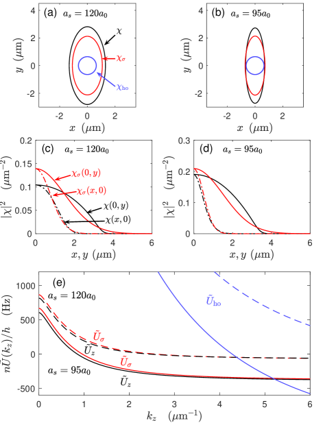
In Fig. 3(a)-(d) we compare results obtained from the 3D and variational theories for the transverse density profile of a 164Dy condensate at a linear density of m for two values of . The lower value of scattering length considered () is close to where the roton excitation softens to zero energy and becomes dynamically unstable (see Sec. III.4). For reference the harmonic oscillator ground state (i.e. quasi-1D result) is also shown. Here we observe that both the 3D and variational eGPE solutions have a much larger transverse width than the harmonic oscillator ground state since the system parameters are outside quasi-1D regime222 We also note that the case in Figs. 3(b) and (d) has , well-satisfying the requirement established in Ref. Edler et al. (2017) for the quantum fluctuations to be described by the 3D formalism we use here.. We also note that while the confining potential is isotropic the condensates exhibits magnetostriction, i.e. significantly elongates in the -direction compared to the -direction.
In Fig. 3(e) we compare the effective 1D -space interaction kernel for the various theories. While the uniform ground state only depends on the value of the kernel at (27), the excitations are sensitive to its non-zero behaviour (29). Our results show that our approximate kernel closely matches that obtained from the full 3D eGPE solution. In comparison, the quasi-1D kernel based on the harmonic oscillator ground state (see Sec. II.2.5) is a poor approximation.
III.3 Fully trapped ground states
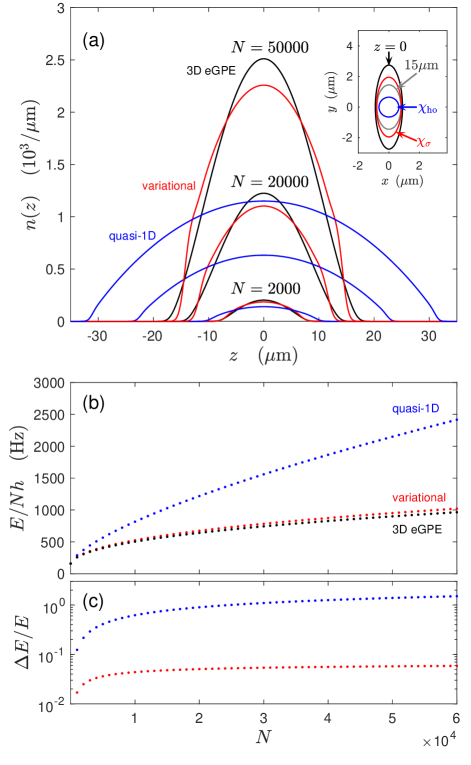
In Fig. 4 we present results for ground states with axial confinement. The line density profiles of the solutions reveal that the variational theory is in reasonable agreement with the 3D eGPE solution, although it generally tends to have a lower peak density. Except for small atom numbers , for which the interaction effects are negligible, the quasi-1D case is in poor agreement with the other theories. A significant difference between the variational and the 3D result arises because the variational solution has the separable form , and thus has the same transverse profile for all . At higher we can see that this not a good approximation to the 3D solution: The transverse profile at (where the density is highest) is more strongly affected by interactions (larger average width and anisotropy) than it is for higher values of [ see inset to Fig. 4(a)]. For the case of condensates with contact interactions an effective 1D theory has been developed that allows the transverse profile to vary slowly with (see Ref. Salasnich et al. (2002)). Such a theory for could be developed for the dipolar case, although we do not pursue this here (also see Knight et al. (2019)). In Fig. 4(b) and (c) we compare the ground state energy, observing that over the wide parameter regime considered the variational prediction for the energy is typically within a few percent of the full 3D solution.
III.4 Uniform system excitations: Roton softening
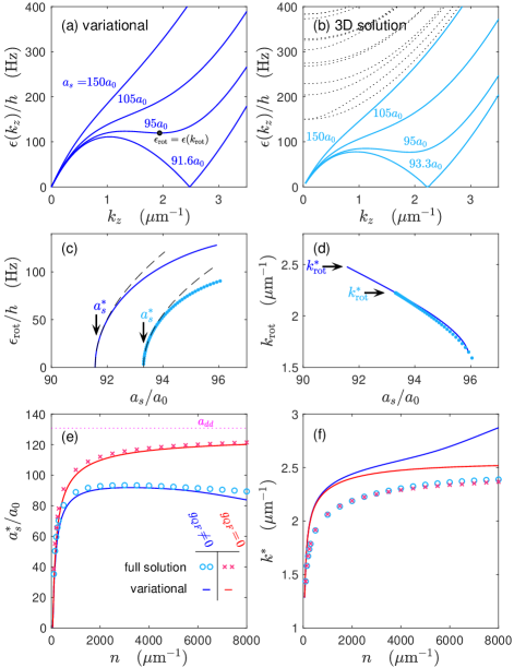
In Figs. 5(a) and (b) we compare the predictions of the variational and 3D theories for the spectrum of a uniform case as is varied. In these results we see that a roton (i.e. a local minimum in the excitation dispersion relation) appears for and lowers in energy as is further decreased. Our calculations predict that the roton hits zero energy at the critical value of scattering length with () according the variational (3D) theory for the density considered. In general we find that the variational theory predicts a lower value of than the 3D result [also see Figs. 5(c) and (e)]. For the uniform state is dynamically unstable.
Identifying the local minimum in the dispersion relation with the roton energy and wavevector [see Fig. 5(a)], we can monitor the behavior of the roton as varies in Figs. 5(c) and (d). The roton energy is seen to soften to zero as for above but close to Chomaz et al. (2018). The roton wave vector tends to increase as decreases, and obtains the value at the critical point . We observe that the variational theory predicts to be larger than that obtained from the 3D theory, however the values of both theories are similar at the same values [see Fig. 5(d)]. We note that our results show that the roton wave vector occurs at a value slightly higher than the inverse harmonic oscillator length along the dipole direction, i.e. m, similar to the observations of experiments Chomaz et al. (2018).
In Figs. 5(e) and (f) we examine the values of and for a range of system densities. We also include results without the quantum fluctuation term. For small , the quantum fluctuations have a small effect and the theories make similar predictions333 The results for m on Figs. 5(e) and (f) have , and the 3D treatment of quantum fluctuations is inappropriate. A quantitative treatment of this regime is outside the scope of this work.. However, in general we find that is larger when the quantum fluctuation term is neglected. We understand this arises because the quantum fluctuations effectively act as a repulsive interaction and tend to stabilize (i.e. lift the energy) of the roton. Thus with quantum fluctuations a lower value is needed to destabilize the condensate. We also find that as a function of has a maximum when quantum fluctuations are included. In contrast without quantum fluctuations monotonically increases with , slowly approaching the value in the large density limit.
IV Conclusions and outlook
In this paper we have reported the development of a simple theory for a dipolar condensate in an elongated confining potential. Our main result is the effective 1D variational eGPE for stationary states, and the associated BdG theory of its collective excitations. This theory is practical to solve with modest computational resources, yet provides a good quantitative description of the full 3D solution.
In the application of our theory we have focused on the typical density, interaction and trap parameter regimes used in current experiments. For example, the rotons observed in the experiments of Chomaz et al. Chomaz et al. (2018) occurred (prior to structure formation occurring) in an elongated system with linear densities in the range m-1. This regime is well-beyond where the quasi-1D approximation is valid. Using our theory we have predicted the scattering length and roton wave vector at the point where roton softens to zero energy as a function of system density. Our results show that quantum fluctuations lower the value of and cause it to have a non-monotonic dependence on density. These predictions could be investigated in future experiments and may relate to the non-monotonic dependence of the value of where the supersolid transition was observed [see Fig. 1(g) of Ref. Chomaz et al. (2019)].
Here we have restricted our focus to the regime where the system does not develop density modulations, which tends to occur at lower values of (e.g., after the roton softens and causes a dynamic instability). Such modulations can indicate the onset of a supersolid state, as has been observed in three recent experiments working with dipolar condensates in elongated trapping potentials. So far theoretical studies of the ground states and their excitations of these modulated states required large scale numerical methods for cases with (see Refs. Tanzi et al. (2019a); Böttcher et al. (2019b); Chomaz et al. (2019); Tanzi et al. (2019b); Guo et al. (2019); Natale et al. (2019)) and without (see Roccuzzo and Ancilotto (2019)) axial confinement. Our theory can treat such modulated states, but a full and systematic treatment of this is beyond the current scope and will be examined in future work.
Acknowledgements.
We acknowledge the contribution of NZ eScience Infrastructure (NeSI) high-performance computing facilities, support from the Marsden Fund of the Royal Society of New Zealand, and valuable discussions with F. Ferlaino and L. Chomaz.References
- Griesmaier et al. (2005) Axel Griesmaier, Jörg Werner, Sven Hensler, Jürgen Stuhler, and Tilman Pfau, “Bose-Einstein condensation of chromium,” Phys. Rev. Lett. 94, 160401 (2005).
- Pasquiou et al. (2011) B. Pasquiou, G. Bismut, E. Maréchal, P. Pedri, L. Vernac, O. Gorceix, and B. Laburthe-Tolra, “Spin relaxation and band excitation of a dipolar Bose-Einstein condensate in 2D optical lattices,” Phys. Rev. Lett. 106, 015301 (2011).
- Lu et al. (2011) Mingwu Lu, Nathaniel Q. Burdick, Seo Ho Youn, and Benjamin L. Lev, “Strongly dipolar Bose-Einstein condensate of dysprosium,” Phys. Rev. Lett. 107, 190401 (2011).
- Lu et al. (2012) Mingwu Lu, Nathaniel Q. Burdick, and Benjamin L. Lev, “Quantum degenerate dipolar Fermi gas,” Phys. Rev. Lett. 108, 215301 (2012).
- Aikawa et al. (2012) K. Aikawa, A. Frisch, M. Mark, S. Baier, A. Rietzler, R. Grimm, and F. Ferlaino, “Bose-Einstein condensation of erbium,” Phys. Rev. Lett. 108, 210401 (2012).
- Chomaz et al. (2018) L. Chomaz, R. M. W. van Bijnen, D. Petter, G. Faraoni, S. Baier, J. H. Becher, M. J. Mark, F. Wächtler, L. Santos, and F. Ferlaino, “Observation of roton mode population in a dipolar quantum gas,” Nat. Phys. 14, 442 (2018).
- Petter et al. (2019) D. Petter, G. Natale, R. M. W. van Bijnen, A. Patscheider, M. J. Mark, L. Chomaz, and F. Ferlaino, “Probing the roton excitation spectrum of a stable dipolar Bose gas,” Phys. Rev. Lett. 122, 183401 (2019).
- Landau (1941) L. D. Landau, “The theory of superfluidity of helium II,” J. Phys. (Mosc.) 5, 71 (1941).
- Santos et al. (2003) L. Santos, G. V. Shlyapnikov, and M. Lewenstein, “Roton-maxon spectrum and stability of trapped dipolar Bose-Einstein condensates,” Phys. Rev. Lett. 90, 250403 (2003).
- Ronen et al. (2007) Shai Ronen, Daniele C. E. Bortolotti, and John L. Bohn, “Radial and angular rotons in trapped dipolar gases,” Phys. Rev. Lett. 98, 030406 (2007).
- Blakie et al. (2012) P. B. Blakie, D. Baillie, and R. N. Bisset, “Roton spectroscopy in a harmonically trapped dipolar Bose-Einstein condensate,” Phys. Rev. A 86, 021604 (2012).
- Corson et al. (2013a) John P. Corson, Ryan M. Wilson, and John L. Bohn, “Stability spectroscopy of rotons in a dipolar Bose gas,” Phys. Rev. A 87, 051605 (2013a).
- Corson et al. (2013b) John P. Corson, Ryan M. Wilson, and John L. Bohn, “Geometric stability spectra of dipolar Bose gases in tunable optical lattices,” Phys. Rev. A 88, 013614 (2013b).
- Jona-Lasinio et al. (2013) M. Jona-Lasinio, K. Łakomy, and L. Santos, “Time-of-flight roton spectroscopy in dipolar Bose-Einstein condensates,” Phys. Rev. A 88, 025603 (2013).
- Bisset and Blakie (2013) R. N. Bisset and P. B. Blakie, “Fingerprinting rotons in a dipolar condensate: Super-poissonian peak in the atom-number fluctuations,” Phys. Rev. Lett. 110, 265302 (2013).
- Baillie and Blakie (2015) D Baillie and P B Blakie, “A general theory of flattened dipolar condensates,” New J. Phys 17, 033028 (2015).
- Roccuzzo and Ancilotto (2019) Santo Maria Roccuzzo and Francesco Ancilotto, “Supersolid behavior of a dipolar Bose-Einstein condensate confined in a tube,” Phys. Rev. A 99, 041601 (2019).
- Kadau et al. (2016) Holger Kadau, Matthias Schmitt, Matthias Wenzel, Clarissa Wink, Thomas Maier, Igor Ferrier-Barbut, and Tilman Pfau, “Observing the Rosensweig instability of a quantum ferrofluid,” Nature 530, 194–197 (2016).
- Ferrier-Barbut et al. (2016) Igor Ferrier-Barbut, Holger Kadau, Matthias Schmitt, Matthias Wenzel, and Tilman Pfau, “Observation of quantum droplets in a strongly dipolar Bose gas,” Phys. Rev. Lett. 116, 215301 (2016).
- Bisset et al. (2016) R. N. Bisset, R. M. Wilson, D. Baillie, and P. B. Blakie, “Ground-state phase diagram of a dipolar condensate with quantum fluctuations,” Phys. Rev. A 94, 033619 (2016).
- Chomaz et al. (2016) L. Chomaz, S. Baier, D. Petter, M. J. Mark, F. Wächtler, L. Santos, and F. Ferlaino, “Quantum-fluctuation-driven crossover from a dilute Bose-Einstein condensate to a macrodroplet in a dipolar quantum fluid,” Phys. Rev. X 6, 041039 (2016).
- Schmitt et al. (2016) Matthias Schmitt, Matthias Wenzel, Fabian Böttcher, Igor Ferrier-Barbut, and Tilman Pfau, “Self-bound droplets of a dilute magnetic quantum liquid,” Nature 539, 259 (2016).
- Böttcher et al. (2019a) Fabian Böttcher, Matthias Wenzel, Jan-Niklas Schmidt, Mingyang Guo, Tim Langen, Igor Ferrier-Barbut, Tilman Pfau, Raúl Bombín, Joan Sánchez-Baena, Jordi Boronat, and Ferran Mazzanti, “Dilute dipolar quantum droplets beyond the extended Gross-Pitaevskii equation,” Phys. Rev. Research 1, 033088 (2019a).
- Böttcher et al. (2019b) Fabian Böttcher, Jan-Niklas Schmidt, Matthias Wenzel, Jens Hertkorn, Mingyang Guo, Tim Langen, and Tilman Pfau, “Transient supersolid properties in an array of dipolar quantum droplets,” Phys. Rev. X 9, 011051 (2019b).
- Tanzi et al. (2019a) L. Tanzi, E. Lucioni, F. Famà, J. Catani, A. Fioretti, C. Gabbanini, R. N. Bisset, L. Santos, and G. Modugno, “Observation of a dipolar quantum gas with metastable supersolid properties,” Phys. Rev. Lett. 122, 130405 (2019a).
- Wächtler and Santos (2016) F. Wächtler and L. Santos, “Quantum filaments in dipolar Bose-Einstein condensates,” Phys. Rev. A 93, 061603(R) (2016).
- Baillie et al. (2017) D. Baillie, R. M. Wilson, and P. B. Blakie, “Collective excitations of self-bound droplets of a dipolar quantum fluid,” Phys. Rev. Lett. 119, 255302 (2017).
- Lee et al. (2018) Au-Chen Lee, D. Baillie, R. N. Bisset, and P. B. Blakie, “Excitations of a vortex line in an elongated dipolar condensate,” Phys. Rev. A 98, 063620 (2018).
- Salasnich et al. (2002) L. Salasnich, A. Parola, and L. Reatto, “Effective wave equations for the dynamics of cigar-shaped and disk-shaped Bose condensates,” Phys. Rev. A 65, 043614 (2002).
- Edler et al. (2017) D. Edler, C. Mishra, F. Wächtler, R. Nath, S. Sinha, and L. Santos, “Quantum fluctuations in quasi-one-dimensional dipolar bose-einstein condensates,” Phys. Rev. Lett. 119, 050403 (2017).
- Lima and Pelster (2011) Aristeu R. P. Lima and Axel Pelster, “Quantum fluctuations in dipolar Bose gases,” Phys. Rev. A 84, 041604 (2011).
- Sinha and Santos (2007) S. Sinha and L. Santos, “Cold dipolar gases in quasi-one-dimensional geometries,” Phys. Rev. Lett. 99, 140406 (2007).
- Deuretzbacher et al. (2010) F. Deuretzbacher, J. C. Cremon, and S. M. Reimann, “Ground-state properties of few dipolar bosons in a quasi-one-dimensional harmonic trap,” Phys. Rev. A 81, 063616 (2010).
- Deuretzbacher et al. (2013) F. Deuretzbacher, J. C. Cremon, and S. M. Reimann, “Erratum: Ground-state properties of few dipolar bosons in a quasi-one-dimensional harmonic trap,” Phys. Rev. A 87, 039903 (2013).
- Giovanazzi and O’Dell (2004) S. Giovanazzi and D.H.J. O’Dell, “Instabilities and the roton spectrum of a quasi-1D Bose-Einstein condensed gas with dipole-dipole interactions,” Eur. Phys. J. D 31, 439–445 (2004).
- Ronen et al. (2006) Shai Ronen, Daniele C. E. Bortolotti, and John L. Bohn, “Bogoliubov modes of a dipolar condensate in a cylindrical trap,” Phys. Rev. A 74, 013623 (2006).
- Giovanazzi et al. (2002) Stefano Giovanazzi, Axel Görlitz, and Tilman Pfau, “Tuning the dipolar interaction in quantum gases,” Phys. Rev. Lett. 89, 130401 (2002).
- Tang et al. (2018) Yijun Tang, Wil Kao, Kuan-Yu Li, and Benjamin L. Lev, “Tuning the dipole-dipole interaction in a quantum gas with a rotating magnetic field,” Phys. Rev. Lett. 120, 230401 (2018).
- Lu et al. (2010) H.-Y. Lu, H. Lu, J.-N. Zhang, R.-Z. Qiu, H. Pu, and S. Yi, “Spatial density oscillations in trapped dipolar condensates,” Phys. Rev. A 82, 023622 (2010).
- Bao et al. (2010) Weizhu Bao, Yongyong Cai, and Hanquan Wang, “Efficient numerical methods for computing ground states and dynamics of dipolar Bose-Einstein condensates,” J. Comput. Phys. 229, 7874 (2010).
- Antoine et al. (2017) Xavier Antoine, Antoine Levitt, and Qinglin Tang, “Efficient spectral computation of the stationary states of rotating Bose-Einstein condensates by preconditioned nonlinear conjugate gradient methods,” J. Comput. Phys. 343, 92 (2017).
- Knight et al. (2019) Mitchell J. Knight, Thomas Bland, Nick G. Parker, and Andy M. Martin, “Improved low-dimensional wave equations for cigar-shaped and disk-shaped dipolar Bose-Einstein condensates,” (2019), arXiv:1908.02395 [cond-mat.quant-gas] .
- Chomaz et al. (2019) L. Chomaz, D. Petter, P. Ilzhöfer, G. Natale, A. Trautmann, C. Politi, G. Durastante, R. M. W. van Bijnen, A. Patscheider, M. Sohmen, M. J. Mark, and F. Ferlaino, “Long-lived and transient supersolid behaviors in dipolar quantum gases,” Phys. Rev. X 9, 021012 (2019).
- Tanzi et al. (2019b) L. Tanzi, S. M. Roccuzzo, E. Lucioni, F. Famà, A. Fioretti, C. Gabbanini, G. Modugno, A. Recati, and S. Stringari, “Supersolid symmetry breaking from compressional oscillations in a dipolar quantum gas,” Nature 574, 382 (2019b).
- Guo et al. (2019) Mingyang Guo, Fabian Böttcher, Jens Hertkorn, Jan-Niklas Schmidt, Matthias Wenzel, Hans Peter Büchler, Tim Langen, and Tilman Pfau, “The low-energy goldstone mode in a trapped dipolar supersolid,” Nature 574, 386 (2019).
- Natale et al. (2019) G. Natale, R. M. W. van Bijnen, A. Patscheider, D. Petter, M. J. Mark, L. Chomaz, and F. Ferlaino, “Excitation spectrum of a trapped dipolar supersolid and its experimental evidence,” Phys. Rev. Lett. 123, 050402 (2019).