Fast and accurate approximations to fractional powers of operators

Abstract.

In this paper we consider some rational approximations to the fractional powers of self-adjoint positive operators, arising from the Gauss-Laguerre rules. We derive practical error estimates that can be used to select a priori the number of Laguerre points necessary to achieve a given accuracy. We also present some numerical experiments to show the effectiveness of our approaches and the reliability of the estimates.

1. Introduction

The numerical solution of problems involving fractional diffusion can lead to the computation of fractional powers of unbounded operators. For instance, denoting by $\Delta$ the standard Laplace operator and taking $\alpha\in(0,1),$ the fractional Laplace equation

(1) $$(-\Delta)^{\alpha}u=f$$

on a bounded Lipschitz domain subject to Dirichlet boundary conditions can be solved by computing

(2) $$\sum_{j=1}^{+\infty}\mu_{j}^{-\alpha}\langle f,\varphi_{j}\rangle\varphi_{j},$$

where $\mu_{j}$ and $\varphi_{j}$ are the eigenvalues and the eigenfunctions of $-\Delta,$ respectively, and $\langle\cdot,\cdot\rangle$ denotes the $L^{2}$-inner product. In practice, in this situation the fractional derivative can be identified by the fractional power. Keeping in mind this kind of applications, in this work we are interested in the numerical approximation of ${\mathcal{L}}^{-\alpha},\alpha\in(0,1).$ Here ${\mathcal{L}}$ is a self-adjoint positive operator acting in an Hilbert space ${\mathcal{H}}$ in which the eigenfunctions of ${\mathcal{L}}$ form an orthonormal basis of ${\mathcal{H}},$ so that ${\mathcal{L}}^{-\alpha}$ can be written through the spectral decomposition of ${\mathcal{L}}$ as in (2).

In recent years, this problem has been studied by many authors. Due to the properties of the function $\lambda^{-\alpha},\lambda\in[\ell,+\infty),\ell>0,$ the most effective approaches are those based on a rational approximation of this function. In the continuous setting of unbounded operators, methods based on the best uniform rational approximation (BURA) of functions closely related to $\lambda^{-\alpha}$ have been considered, for example, in [10, 11, 12, 13] by using a modified version of the Remez algorithm. Another class of methods relies on quadrature rules for the integral representation of $\lambda^{-\alpha}$ [2, 3, 4, 7, 20, 21]. Very recently, time stepping methods for a parabolic reformulation of the fractional diffusion equation (1) given in [22] have also been interpreted in [14] as a rational approximation of $\lambda^{-\alpha}.$

In this paper, starting from the integral representation given in [7, Eq. (4)]

(3) $$\mathcal{L}^{-\alpha}=\frac{2\sin(\alpha\pi)}{\pi}\int_{0}^{+\infty}t^{2\alpha-1}({\mathcal{I}}+t^{2}\mathcal{L})^{-1}dt,\qquad\alpha\in(0,1),$$

where ${\mathcal{I}}$ is the identity operator in ${\mathcal{H}},$ after suitable changes of variables we consider an alternative rational approximation based on the truncated Gauss-Laguerre rule. In order to construct the truncated approach, we exploit the error analysis of the standard Gauss-Laguerre rule based on the theory of analytic functions originally introduced in [5]. We are able to show that in the operator norm the error decay like

$$\exp(-cm^{1/2})$$

where $m$ is the number of inversions and $c=3.6\alpha^{1/2}$ (cf. (48)). In this view, the formula seems to be competitive with the Sinc quadrature studied in [7] in which $c=\pi(1-\alpha)^{1/2}\alpha^{1/2}$ by Remark 3.1 of the same paper. However, it appears to be slightly slower than that based on the analysis given in [18] and related to the BURA approach in which $c=2\pi(1-\alpha)^{1/2}$ although the approach presented here does not suffer from the instability of Remez algorithm.

We also present a further modification of the truncated Gauss-Laguerre rule, called equalized rule, that allows to further reduce the number of inversions to achieve the same accuracy, especially when $\alpha\leq 1/2.$

The paper is structured as follows. In Section 2 we present the Gauss-Laguerre approach. In Sections 3-4, starting from the error analysis based on the theory of analytic functions, we present the error estimate attainable with the Gauss-Laguerre approach for the approximation of $\lambda^{-\alpha}.$ The analysis is then extended in Section 5 to the case of the operator ${\mathcal{L}}^{-\alpha}.$ Finally, the truncated rules are proposed in Section 6.

2. The Gauss-Laguerre approach

As already said in the introduction, we start from the integral representation given in (3). Setting $y=\ln t$ we obtain

(4) $$\mathcal{L}^{-\alpha}=\frac{2\sin(\alpha\pi)}{\pi}\int_{-\infty}^{+\infty}e^{{2\alpha}y}({\mathcal{I}}+e^{2y}\mathcal{L})^{-1}dy,\qquad\alpha\in(0,1).$$

Now we consider separately the two integrals

$$\int_{-\infty}^{0}e^{{2\alpha}y}({\mathcal{I}}+e^{2y}\mathcal{L})^{-1}dy,\quad\int_{0}^{+\infty}e^{{2\alpha}y}({\mathcal{I}}+e^{2y}\mathcal{L})^{-1}dy$$

and consider the changes of variable ${2\alpha}y=-x$ and $2(1-\alpha)y=x$ respectively, to obtain

$$\int_{-\infty}^{0}e^{{2\alpha}y}({\mathcal{I}}+e^{2y}\mathcal{L})^{-1}dy = \frac{1}{2\alpha}\int_{0}^{+\infty}e^{-x}({\mathcal{I}}+e^{-x/\alpha}\mathcal{L})^{-1}dx,$$

$$\int_{0}^{+\infty}e^{{2\alpha}y}({\mathcal{I}}+e^{2y}\mathcal{L})^{-1}dy = \frac{1}{2(1-\alpha)}\int_{0}^{+\infty}e^{-x}(e^{-x/(1-\alpha)}{\mathcal{I}}+\mathcal{L})^{-1}dx.$$

Consequently, setting

(5) $$I^{(1)}(\lambda) := \int_{0}^{+\infty}e^{-x}(1+e^{-x/\alpha}\lambda)^{-1}dx,$$

(6) $$I^{(2)}(\lambda) := \int_{0}^{+\infty}e^{-x}(e^{-x/(1-\alpha)}+\lambda)^{-1}dx,$$

the operator in (4) can be written as

(7) $$\mathcal{L}^{-\alpha}=\frac{\sin(\alpha\pi)}{\alpha\pi}I^{(1)}(\mathcal{L})+\frac{\sin(\alpha\pi)}{(1-\alpha)\pi}I^{(2)}(\mathcal{L}).$$

It is easy to check that $I^{(1)}(\mathcal{L})\rightarrow\mathcal{I}$ as $\alpha\rightarrow 0$ and $I^{(2)}(\mathcal{L})\rightarrow\mathcal{L}^{-1}$ as $\alpha\rightarrow 1.$

By applying the $n$-point Gauss-Laguerre rule to both integrals with respect to the weight function $\omega(x)=e^{-x},$ with weights $w_{j}^{(n)}$ and nodes $\vartheta_{j}^{(n)}$ (in ascending order), we obtain the following $(2n-1,2n)$ rational approximation

(8) $$\mathcal{L}^{-\alpha}\approx\frac{\sin(\alpha\pi)}{\alpha\pi}R_{n-1,n}^{(1)}(\mathcal{L})+\frac{\sin(\alpha\pi)}{(1-\alpha)\pi}R_{n-1,n}^{(2)}(\mathcal{L})=:R_{2n-1,2n}(\mathcal{L}),$$

where

$$R_{n-1,n}^{(1)}(\lambda) = \sum_{j=1}^{n}w_{j}^{(n)}\left(1+e^{-{\vartheta_{j}^{(n)}}/{\alpha}}\lambda\right)^{-1},$$

$$R_{n-1,n}^{(2)}(\lambda) = \sum_{j=1}^{n}w_{j}^{(n)}\left(e^{-{\vartheta_{j}^{(n)}}/{(1-\alpha)}}+\lambda\right)^{-1}.$$

Clearly, formula (8) implies that using $n$ points we have to perform $2n$ inversions.

3. Error analysis for a general function

In order to obtain an estimate of the error for the rational approximation defined in (8), we consider the approach introduced in [5] and based on the theory of analytic functions. Assuming to work with a general function $f$ and then to consider the $n$-point Gauss-Laguerre rule $I_{n}(f)$ for

$$I(f)=\int_{0}^{+\infty}e^{-x}f(x)dx,$$

we define the remainder as $E_{n}(f)=I(f)-I_{n}(f)$. For any given $R>1$, the equation

$$\operatorname{Re}(\sqrt{-z})=\ln R$$

represents a parabola in the complex plane, that we denote by $\Gamma_{R}$, symmetric with respect to the real axis, with vertex in $-\left(\ln R\right)^{2}$ and convexity oriented towards the positive real axis. By writing $z=a+ib$, the above equation reads

$$a=\left(b^{2}-4\left(\ln R\right)^{4}\right)\frac{1}{4\left(\ln R\right)^{2}}.$$

The parabola degenerates to $[0,+\infty)$ as $R\rightarrow 1$. The theory given in [5] states that, if for a given $R$ the function $f$ is analytic on or within $\Gamma_{R}$ except for a pair of simple poles, $z_{0}$ and its conjugate $\overline{z_{0}}$, then

(9) $$E_{n}(f)\approx-4\pi\operatorname{Re}\left\{re^{-z_{0}}\left[\exp\left(\sqrt{-z_{0}}\right)\right]^{-2\sqrt{\bar{n}}}\right\},$$

where $r$ is the residue of $f(z)$ at $z_{0}$ and

(10) $$\bar{n}=4n+2.$$

This result follows from the fact that $E_{n}(f)$ can be written as a contour integral

$$E_{n}(f)=\frac{1}{2\pi i}\int_{\Gamma}\frac{q_{n}(z)}{L_{n}(z)}f(z)dz,$$

where $L_{n}(z)$ is the Laguerre polynomial, $q_{n}(z)$ is the so-called associated function defined by

$$q_{n}(z)=\int\nolimits_{0}^{+\infty}\frac{e^{-x}L_{n}(x)}{z-x}dx,\quad z\notin[0,+\infty),$$

and $\Gamma$ is a contour containing $[0,+\infty)$ with the additional property that no singularity of $f(z)$ lies on or within this contour (see [8, §4.6] for a background).

Denoting by $C_{1}$ and $C_{2}$ two arbitrary small circles surrounding the two poles the idea is then to define $\Gamma=\Gamma_{R}\cup C_{1}\cup C_{2}$. In order to run this contour in the counterclockwise direction, one can artificially add three line segments as shown in Figure 1 to connect the circles with the parabola. Then, following the black and the red arrows, the integrals along the line segments cancel and we obtain

(11) $$E_{n}(f)=\frac{1}{2\pi i}\left\{\int_{\Gamma_{R}}-\int_{C_{1}}-\int_{C_{2}}\right\}\frac{q_{n}(z)}{L_{n}(z)}f(z)dz.$$

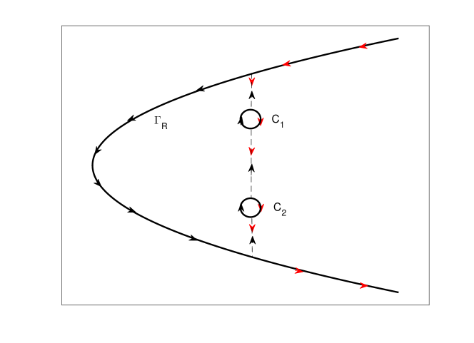
Figure 1. Contour chosen for a function $f$ analytic on or within the parabola $\Gamma_{R}$ with the exception of two simple and conjugated poles located inside $C_{1}$ and $C_{2},$ respectively.

At this point, the estimate is based on the relation given in [9, Eq. (5.4)], namely

$$\frac{q_{n}(z)}{L_{n}(z)}=2\pi e^{-z}\left[\exp\left(\sqrt{-z}\right)\right]^{-2\sqrt{\bar{n}}}\left(1+O\left(\frac{1}{n}\right)\right),\quad z\notin[0,+\infty),$$

Since

(12) $$\left[\exp\left(\operatorname{Re}\left(\sqrt{-z}\right)\right)\right]^{-2\sqrt{\bar{n}}}=R^{-2\sqrt{\bar{n}}},\quad\text{\ for }z\in\Gamma_{R},$$

the contribution on the parabola is given by

$$\frac{1}{2\pi i}\int_{\Gamma_{R}}\frac{q_{n}(z)}{L_{n}(z)}f(z)dz=R^{-2\sqrt{\bar{n}}}$$

$$\times \frac{1}{i}\int_{\Gamma_{R}}e^{-z}\left[\exp\left(i\operatorname{Im}\left(\sqrt{-z}\right)\right)\right]^{-2\sqrt{\bar{n}}}f(z)dz\left(1+O\left(\frac{1}{n}\right)\right):=\phi(n).$$

In addition, using the residue theorem we have

$$\frac{1}{2\pi i}\left\{\int_{C_{1}}+\int_{C_{2}}\right\}e^{-z}\left[\exp\left(\sqrt{-z}\right)\right]^{-2\sqrt{\bar{n}}}f(z)dz$$

$$= \operatorname{Res}\left(e^{-z}\left[\exp\left(\sqrt{-z}\right)\right]^{-2\sqrt{\bar{n}}}f(z),z_{0}\right)$$

$$+ \operatorname{Res}\left(e^{-z}\left[\exp\left(\sqrt{-z}\right)\right]^{-2\sqrt{\bar{n}}}f(z),\overline{z_{0}}\right)$$

$$= 2\operatorname{Re}\left(\operatorname{Res}\left(e^{-z}\left[\exp\left(\sqrt{-z}\right)\right]^{-2\sqrt{\bar{n}}}f(z),z_{0}\right)\right)$$

$$= 2\operatorname{Re}\left(\operatorname{Res}\left(f(z),z_{0}\right)e^{-z_{0}}\left[\exp\left(\sqrt{-z_{0}}\right)\right]^{-2\sqrt{\bar{n}}}\right).$$

Therefore from (11), by taking into account (3), we obtain

$$E_{n}(f) = -4\pi\operatorname{Re}\left(\operatorname{Res}\left(f(z),z_{0}\right)e^{-z_{0}}\left[\exp\left(\sqrt{-z_{0}}\right)\right]^{-2\sqrt{\bar{n}}}\right)\left(1+O\left(\frac{1}{n}\right)\right)$$

$$+ \phi(n).$$

Obviously, this implies the formula (9) whenever the contribution from the parabola $\Gamma_{R}$ (i.e., $\phi(n)$) can be considered negligible. As for the modulus of the error, observing that

$$\left|\operatorname{Re}\left(\operatorname{Res}\left(f(z),z_{0}\right)e^{-z_{0}}\left[\exp\left(\sqrt{-z_{0}}\right)\right]^{-2\sqrt{\bar{n}}}\right)\right|\leq$$

$$\leq \left|\operatorname{Res}\left(f(z),z_{0}\right)e^{-z_{0}}\right|\left[\exp\left(\operatorname{Re}\left(\sqrt{-z_{0}}\right)\right)\right]^{-2\sqrt{\bar{n}}},$$

we have

$$|E_{n}(f)| \leq 4\pi\left|\operatorname{Res}\left(f(z),z_{0}\right)e^{-z_{0}}\right|\left[\exp\left(\operatorname{Re}\left(\sqrt{-z_{0}}\right)\right)\right]^{-2\sqrt{\bar{n}}}\left(1+O\left(\frac{1}{n}\right)\right)$$

$$+ |\phi(n)|.$$

Since hereafter we assume that

$$\int_{\Gamma_{R}}|e^{-z}f(z)|dz$$

is bounded, from (3) we obtain (see (10) and (12))

$$\frac{\left|\phi(n)\right|}{\left[\exp\left(\operatorname{Re}\left(\sqrt{-z_{0}}\right)\right)\right]^{-2\sqrt{\bar{n}}}}\leq\frac{cR^{-2\sqrt{\bar{n}}}}{\left[\exp\left(\operatorname{Re}\left(\sqrt{-z_{0}}\right)\right)\right]^{-2\sqrt{\bar{n}}}}=O\left(\exp(-n^{1/2})\right)$$

and then

(14) $$|E_{n}(f)|\leq 4\pi\left|\operatorname{Res}\left(f(z),z_{0}\right)e^{-z_{0}}\right|\left[\exp\left(\operatorname{Re}\left(\sqrt{-z_{0}}\right)\right)\right]^{-2\sqrt{\bar{n}}}\left(1+O\left(\frac{1}{n}\right)\right).$$

4. Error analysis for $\lambda^{-\alpha}$

From (7) and (8) and defining

(15) $$\varepsilon_{n}^{(i)}\left(\lambda\right)=\left|I^{(i)}(\lambda)-R_{n-1,n}^{(i)}(\lambda)\right|,\quad i=1,2,$$

we can write

(16) $$\left|\lambda^{-\alpha}-R_{2n-1,2n}(\lambda)\right|\leq\frac{\sin(\alpha\pi)}{\alpha\pi}\varepsilon_{n}^{(1)}\left(\lambda\right)+\frac{\sin(\alpha\pi)}{(1-\alpha)\pi}\varepsilon_{n}^{(2)}\left(\lambda\right).$$

Hence, using the results of the previous section we can develop the error analysis by working separately on the two integrals $I^{(i)}(\lambda)$, $i=1,2.$

4.1. First integral $I^{(1)}(\lambda)$

The function involved in (5) is

(17) $$f(z)=(1+e^{-z/\alpha}\lambda)^{-1},$$

whose poles are given by

$$z_{k}=\alpha\ln\lambda+i(2k+1)\alpha\pi,\quad k\in\mathbb{Z}.$$

They are equally spaced along the line $\operatorname{Re}(z)=\alpha\ln\lambda$, symmetric with respect to the real axis, and the closest to the real axis are $z_{0}=\alpha\ln\lambda+i\alpha\pi$ and $z_{-1}=\overline{z_{0}}$. It is immediate to verify that there exists $R>1$ such that the corresponding parabola $\operatorname{Re}(\left(-z\right)^{1/2})=\ln R$ contains only the poles $z_{0}$ and $\overline{z_{0}}$ in its interior and that such an $R$ satisfies

$$\frac{\alpha}{2}\left(\sqrt{\left(\ln\lambda\right)^{2}+\pi^{2}}-\ln\lambda\right)<\left(\ln R\right)^{2}<\frac{\alpha}{2}\left(\sqrt{\left(\ln\lambda\right)^{2}+9\pi^{2}}-\ln\lambda\right).$$

These bounds follow by imposing $z_{0}\in\Gamma_{R}$ (the left one) and $z_{1}=\alpha\ln\lambda+i3\alpha\pi\in\Gamma_{R}$ (the right one).

In order to apply (14), first we observe that

$$\left(-z_{0}\right)^{1/2} = \left[-\left(\alpha\ln\lambda+i\alpha\pi\right)\right]^{1/2}$$

$$= \sqrt{\frac{\alpha}{2}}\left(\gamma^{-}\left(\lambda\right)-i\gamma^{+}\left(\lambda\right)\right),$$

where

(18) $$\gamma^{\pm}\left(\lambda\right)=\sqrt{\sqrt{\left(\ln\lambda\right)^{2}+\pi^{2}}\pm\ln\lambda}.$$

Then, recalling that $z_{0}/\alpha=\ln\lambda+i\pi,$ we write

$$1+e^{-z/\alpha}\lambda=1-e^{-(z-z_{0})/\alpha}=\frac{z-z_{0}}{\alpha}\sum_{j=0}^{+\infty}\frac{(-1)^{j}(z-z_{0})^{j}}{\alpha^{j}(j+1)!}.$$

In this case, the residue of the function given in (17) at the simple pole $z_{0}$ is given by

$$\operatorname{Res}\left(f(z),z_{0}\right)=\lim_{z\rightarrow z_{0}}\frac{z-z_{0}}{1+e^{-z/\alpha}\lambda}=\alpha.$$

Therefore, from (14) we have

(19) $$\varepsilon_{n}^{(1)}\left(\lambda\right)\leq 4\pi\alpha\lambda^{-\alpha}\exp\left(-\gamma^{-}\left(\lambda\right)\left(2\alpha\bar{n}\right)^{1/2}\right)\left(1+O\left(\frac{1}{n}\right)\right).$$

4.2. Second integral $I^{(2)}(\lambda)$

The function to consider in this case is

$$f(z)=(e^{-z/(1-\alpha)}+\lambda)^{-1},$$

whose poles are given by

$$z_{k}=-(1-\alpha)\ln\lambda+i(2k+1)(1-\alpha)\pi,\quad k\in\mathbb{Z}.$$

The only difference with respect to the integral $I^{(1)}(\lambda)$ is that the poles have now a negative real part. Anyway, as before we can easily find a parabola containing in its interior only the poles $z_{0}=-(1-\alpha)\ln\lambda+i(1-\alpha)\pi$ and its conjugate. We have now

$$\left(-z_{0}\right)^{1/2}=\sqrt{\frac{1-\alpha}{2}}\left(\gamma^{+}\left(\lambda\right)+i\gamma^{-}\left(\lambda\right)\right),$$

where $\gamma^{\pm}\left(\lambda\right)$ are defined in (18). As for the residue at $z_{0}$ we easily find that $\operatorname{Res}\left(f(z),z_{0}\right)=(1-\alpha)/\lambda$. Using again (14) we have

(20) $$\varepsilon_{n}^{(2)}\left(\lambda\right)\leq 4\pi(1-\alpha)\lambda^{-\alpha}\exp\left(-\gamma^{+}\left(\lambda\right)\left(2(1-\alpha)\overline{n}\right)^{1/2}\right)\left(1+O\left(\frac{1}{n}\right)\right).$$

Finally, plugging in (16) the bounds (19) and (20) we have the following result.

Proposition 1.

Let $\gamma^{\pm}\left(\lambda\right)$ be defined in (18) and $\bar{n}=4n+2.$ Denoting by

(21) $$g_{n}^{(1)}(\lambda) := \lambda^{-\alpha}\exp\left(-\gamma^{-}\left(\lambda\right)\left(2\alpha\bar{n}\right)^{1/2}\right),$$

(22) $$g_{n}^{(2)}(\lambda) := \lambda^{-\alpha}\exp\left(-\gamma^{+}\left(\lambda\right)\left(2(1-\alpha)\bar{n}\right)^{1/2}\right)$$

the $\lambda$-dependent factors of $\varepsilon_{n}^{(1)}\left(\lambda\right)$ and $\varepsilon_{n}^{(2)}\left(\lambda\right)$, respectively, then we have

(23) $$\left|\lambda^{-\alpha}-R_{2n-1,2n}(\lambda)\right|\leq 4\sin(\alpha\pi)\left[g_{n}^{(1)}(\lambda)+g_{n}^{(2)}(\lambda)\right]\left(1+O\left(\frac{1}{n}\right)\right).$$

In order to verify the estimate provided in (23), in Figure 2 we consider an example with $\lambda=10.$ Here and below, nodes and weights of the Gauss-Laguerre rule have been computed using the Matlab function GaussLaguerre.m given in [23].

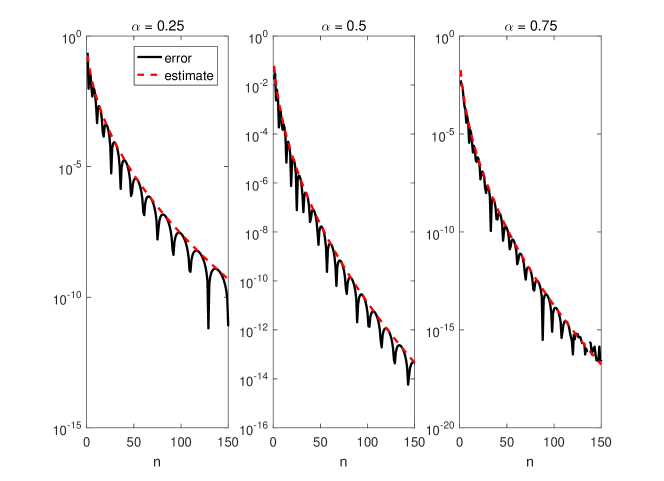
Figure 2. Absolute error and its estimate given by (23) for $\lambda=10.$

5. Error analysis for $\mathcal{L}^{-\alpha}$

For simplicity, from now on we assume that $\sigma(\mathcal{L})\subseteq[1,+\infty).$ Since $\mathcal{L}$ is self-adjoint and positive, regarding the error we have

(24) $$\left\|\mathcal{L}^{-\alpha}-R_{2n-1,2n}(\mathcal{L})\right\|\leq\max_{\lambda\geq 1}\left|\lambda^{-\alpha}-R_{2n-1,2n}(\lambda)\right|,$$

where $\left\|\cdot\right\|$ denotes the operator norm in $\mathcal{H}.$ By (23) we must therefore study the functions $g_{n}^{(i)}(\lambda)$, $i=1,2,$ for $\lambda\geq 1.$ In particular, this means to study the functions $\gamma^{\pm}\left(\lambda\right)$ (see (21) and (22)). By (18), it is immediate to see that $\gamma^{-}\left(\lambda\right)\rightarrow 0$ and $\gamma^{+}\left(\lambda\right)\rightarrow+\infty$ as $\lambda\rightarrow+\infty$. As consequence, the function $g_{n}^{(1)}(\lambda)$ has exactly one maximum at a certain $\lambda_{n}>1$, whereas $g_{n}^{(2)}(\lambda)$ is monotone decreasing, independently of $\alpha$ and $n.$ At this point, in order to compute the right hand side in (24) the first step consists in finding the point of maximum $\lambda_{n}.$

Proposition 2.

Let $\lambda_{n}$ be the maximum of the function $g_{n}^{(1)}(\lambda).$ Then, for $n$ large enough

$$\lambda_{n}=\widetilde{\lambda}_{n}\left(1+O\left(n^{-1/3}\right)\right),$$

where

$$\widetilde{\lambda}_{n}=\exp\left(\left(\left(\frac{\overline{n}\pi^{2}}{4\alpha}\right)^{2/3}-\pi^{2}\right)^{1/2}\right).$$

Proof.

By imposing $\displaystyle{\frac{d}{d\lambda}}g_{n}^{(1)}(\lambda)=0$, after some manipulation we arrive at the equation

(25) $$\frac{\sqrt{\left(\ln\lambda\right)^{2}+\pi^{2}}-\ln\lambda}{\left(\ln\lambda\right)^{2}+\pi^{2}}=\frac{2\alpha}{\bar{n}},$$

whose solution is denoted by $\lambda_{n}.$ Since

$$\frac{\sqrt{\left(\ln\lambda\right)^{2}+\pi^{2}}-\ln\lambda}{\left(\ln\lambda\right)^{2}+\pi^{2}} = \frac{\pi^{2}}{\left(\left(\ln\lambda\right)^{2}+\pi^{2}\right)\left(\sqrt{\left(\ln\lambda\right)^{2}+\pi^{2}}+\ln\lambda\right)}$$

$$\geq \frac{\pi^{2}}{2\left(\left(\ln\lambda\right)^{2}+\pi^{2}\right)^{3/2}},$$

by (25) we first observe that there exists a constant $c$ independent of $n$ such that $\left(\ln\lambda_{n}\right)^{3}\geq cn$, for $n$ large enough. Writing

$$\ln\lambda=s\sqrt{\left(\ln\lambda\right)^{2}+\pi^{2}},$$

where

(27) $$s=s(\lambda)=\frac{1}{\sqrt{1+\left(\frac{\pi}{\ln\lambda}\right)^{2}}},$$

by (25) and (5) we obtain

$$\frac{\pi^{2}}{\left(\left(\ln\lambda\right)^{2}+\pi^{2}\right)^{3/2}\left(1+s\right)}=\frac{2\alpha}{\overline{n}}.$$

As consequence

$$\lambda_{n}=\exp\left(\left(\left(\frac{\overline{n}\pi^{2}}{2\alpha(1+s(\lambda_{n}))}\right)^{2/3}-\pi^{2}\right)^{1/2}\right).$$

Since asymptotically $\left(\ln\lambda_{n}\right)^{2}\geq cn^{2/3}$, from (27) we have

$$s(\lambda_{n})=1+O(n^{-2/3})$$

and therefore

(28) $$\lambda_{n}=\exp\left(\left(\left(\frac{\overline{n}\pi^{2}}{4\alpha}\right)^{2/3}-\pi^{2}+O(1)\right)^{1/2}\right).$$

Writing

$$\left(\left(\frac{\overline{n}\pi^{2}}{4\alpha}\right)^{2/3}-\pi^{2}+O(1)\right)^{1/2}=\left(\left(\frac{\overline{n}\pi^{2}}{4\alpha}\right)^{2/3}-\pi^{2}\right)^{1/2}+\sigma_{n}$$

we easily find that

$$\sigma_{n}=O\left(n^{-1/3}\right).$$

Finally, we obtain the result since

$$\lambda_{n}=\exp\left(\left(\left(\frac{\overline{n}\pi^{2}}{4\alpha)}\right)^{2/3}-\pi^{2}\right)^{1/2}\right)\exp(\sigma_{n}).$$

∎

This approximation is rather good as it can be observed in Figure 3 where we plot $\ln\lambda_{n}$ and $\ln\widetilde{\lambda}_{n}$ for $n=10,11,\dots,120.$ Here the value of $\lambda_{n}$ which verifies (25) has been numerically computed by using a nonlinear solver.

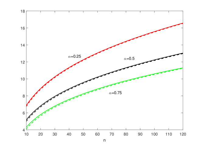
Figure 3. Comparison between $\ln\lambda_{n}$ (solid lines) and $\ln{\tilde{\lambda}_{n}}$ (dahed lines) for $n=10,11,\dots,120$.

Proposition 3.

Let $g_{n}^{(1)}(\lambda)$ and $g_{n}^{(2)}(\lambda)$ be the functions defined in (21) and (22), respectively. Then,

(29) $$\max_{\lambda\geq 1}g_{n}^{(1)}(\lambda) = g_{n}^{(1)}(\lambda_{n})=\exp\left(-3\left(n\alpha^{2}\pi^{2}\right)^{1/3}\right)\left(1+O\left(n^{-1/3}\right)\right),$$

(30) $$\max_{\lambda\geq 1}g_{n}^{(2)}(\lambda) = g_{n}^{(2)}(1)=\exp\left(-\left(8\pi(1-\alpha)n\right)^{1/2}\right)\left(1+O\left(n^{-1/2}\right)\right).$$

Proof.

First of all we need to evaluate $\gamma^{-}\left(\lambda_{n}\right)\left(2\alpha\overline{n}\right)^{1/2}$. Using (18) and (25) we have

$$\left(\gamma^{-}\left(\lambda_{n}\right)\right)^{2}=\frac{2\alpha}{\overline{n}}\left(\left(\ln\lambda_{n}\right)^{2}+\pi^{2}\right).$$

By (28) we also have

(31) $$\left(\ln\lambda_{n}\right)^{2}+\pi^{2}=\left(\frac{\overline{n}\pi^{2}}{4\alpha}\right)^{2/3}+O(1)$$

and hence

$$\gamma^{-}\left(\lambda_{n}\right) = \left(\left(\frac{\alpha}{2\overline{n}}\right)^{1/3}\pi^{4/3}+O(n^{-1})\right)^{1/2}$$

$$= \left(\frac{\alpha}{2\overline{n}}\right)^{1/6}\pi^{2/3}\left(1+O(n^{-2/3})\right).$$

Consequently,

$$\gamma^{-}\left(\lambda_{n}\right)\left(2\alpha\overline{n}\right)^{1/2}=(2\overline{n}\alpha^{2}\pi^{2})^{1/3}\left(1+O(n^{-2/3})\right).$$

Using the result obtained in Proposition 2, we can write

$$\lambda_{n}^{-\alpha} = \exp\left(-\alpha\left(\left(\left(\frac{\overline{n}\pi^{2}}{4\alpha}\right)^{2/3}-\pi^{2}\right)^{1/2}\right)\right)\left(1+O\left(n^{-1/3}\right)\right)$$

$$= \exp\left(-\left(\frac{\overline{n}\alpha^{2}\pi^{2}}{4}\right)^{1/3}\right)\left(1+O\left(n^{-1/3}\right)\right).$$

Therefore, we have

$$g_{n}^{(1)}(\lambda_{n}) = \exp\left(-\left(\frac{\overline{n}\alpha^{2}\pi^{2}}{4}\right)^{1/3}\right)\left(1+O\left(n^{-1/3}\right)\right)$$

$$\times \exp\left(-(2\overline{n}\alpha^{2}\pi^{2})^{1/3}\left(1+O(n^{-2/3})\right)\right)$$

$$= \exp\left(-\left(\overline{n}\alpha^{2}\pi^{2}\right)^{1/3}\left(4^{-1/3}+2^{1/3}\right)\right)\left(1+O\left(n^{-1/3}\right)\right).$$

Finally, recalling that $\overline{n}=4n+2$ we obtain the result.

As for the function $g_{n}^{(2)}(\lambda)$, the situation is much simpler. Indeed, since it is monotone decreasing using (18) and (22) we have that

$$\max_{\lambda\geq 1}g_{n}^{(2)}(\lambda) = g_{n}^{(2)}(1)=\exp\left(-\left(2\pi(1-\alpha)\overline{n}\right)^{1/2}\right)$$

$$= \exp\left(-\left(8\pi(1-\alpha)n\right)^{1/2}\right)\left(1+O\left(n^{-1/2}\right)\right).$$

∎

Finally, we can prove the following result.

Proposition 4.

Let $R_{2n-1,2n}(\mathcal{L})$ be the rational approximation given in (8). Then, with respect to the operator norm in ${\mathcal{H}}$ we have for $n$ large enough

(32) $$\left\|\mathcal{L}^{-\alpha}-R_{2n-1,2n}(\mathcal{L})\right\|\leq 4\sin(\alpha\pi)\exp\left(-3\left(n\alpha^{2}\pi^{2}\right)^{1/3}\right)\left(1+O\left(n^{-1/3}\right)\right).$$

Proof.

First of all, by comparing (29) with (30) for $n$ large enough we can write

$$\frac{g_{n}^{(2)}(1)}{g_{n}^{(1)}(\lambda_{n})}\leq\frac{1}{n}.$$

Therefore,

$$\max_{\lambda\geq 1}\left(g_{n}^{(1)}(\lambda)+g_{n}^{(2)}(\lambda)\right) \leq \max_{\lambda\geq 1}g_{n}^{(1)}(\lambda)+\max_{\lambda\geq 1}g_{n}^{(2)}(\lambda)$$

$$\leq g_{n}^{(1)}(\lambda_{n})+g_{n}^{(2)}(1)$$

$$= g_{n}^{(1)}(\lambda_{n})\left(1+O\left(n^{-1}\right)\right).$$

By Propostion 3 we find the result. ∎

To test the estimate just given in Proposition 4 we work with the operator

(33) $$\mathcal{L}=\left[\operatorname{diag}(1,2,\dots,100)\right]^{8}$$

so that $\sigma(\mathcal{L})\subseteq\left[1,10^{16}\right]$. In Figure 4 we plot the error and its estimate (32) with respect to the number of inversions, that is, $2n.$ From now on, for discrete operators the error is plotted with respect to the Euclidean matrix norm.

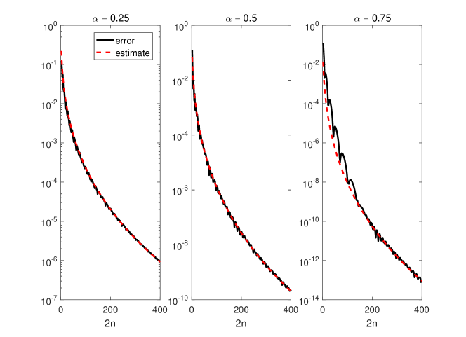
Figure 4. Error and its estimate given by (32) for the operator defined in (33).

Notwithstanding the above result, experimentally (see Figure 5) it is immediate to observe that

$$\max_{\lambda\geq 1}\left(g_{n}^{(1)}(\lambda)+g_{n}^{(2)}(\lambda)\right) \approx \max\left(g_{n}^{(1)}(\lambda_{n}),g_{n}^{(2)}(1)\right).$$

This because the contribution of a function in correspondence of the maximum of the other one is negligible. In order to understand whenever $g_{n}^{(2)}(1)$ may be greater than $g_{n}^{(1)}(\lambda_{n})$ for some values of $n$ and $\alpha$ (as in Figure 5 for $\alpha=0.75$) we just need to compare $g_{n}^{(2)}(1)$ with $g_{n}^{(1)}(1)$.

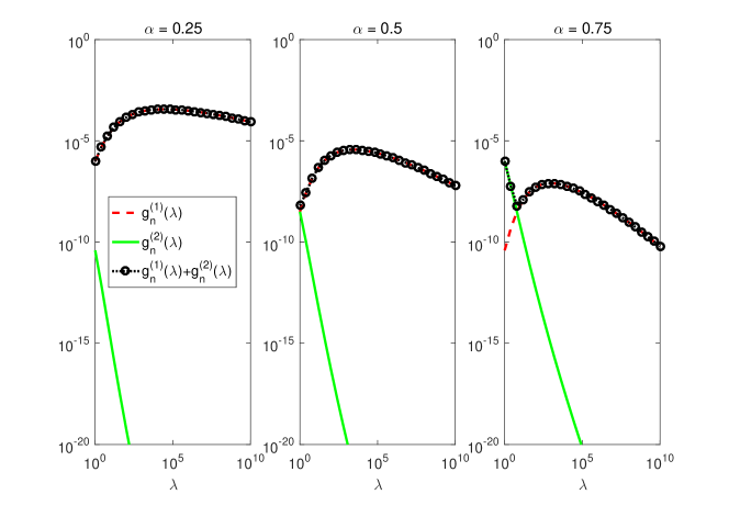
Figure 5. Behavior of the functions $g_{n}^{(1)}(\lambda),g_{n}^{(2)}(\lambda),g_{n}^{(1)}(\lambda)+g_{n}^{(2)}(\lambda)$ for $n=30.$

Using (18), (21) and (22) the equation $g_{n}^{(1)}(1)=g_{n}^{(2)}(1)$ is approximatively equivalent to

$$\exp\left(-\left(2\pi\alpha\overline{n}\right)^{1/2}\right)=\exp\left(-\left(2\pi(1-\alpha)\overline{n}\right)^{1/2}\right),$$

whose solution is $\alpha=1/2$ independently of $n.$ This means that for $\alpha\leq 1/2$

$$\max_{\lambda\geq 1}\left(g_{n}^{(1)}(\lambda)+g_{n}^{(2)}(\lambda)\right)\approx g_{n}^{(1)}(\lambda_{n})$$

and therefore the error decays like $\exp\left(-cn^{1/3}\right)$ for some absolute constant $c$ (cf. (29)), whereas for $\alpha>1/2$ the situation is a bit more complicate. By comparing (29) with (5) we have that asymptotically $g_{n}^{(2)}(1)$ decay faster than $g_{n}^{(1)}(\lambda_{n})$, so, after a certain $n^{\ast}$ the decay rate is still of type $\exp\left(-cn^{1/3}\right)$ also for $\alpha>1/2.$ Anyway, for $n\leq n^{\ast}$ the decay rate is of type $\exp\left(-cn^{1/2}\right).$ The integer $n^{\ast}$ comes from the solution with respect to $n$ of

$$g_{n}^{(1)}(\lambda_{n})=g_{n}^{(2)}(1).$$

Using Proposition 3 we can estimate it by solving

$$\exp\left(-3\left(n\alpha^{2}\pi^{2}\right)^{1/3}\right)=\exp\left(-\left(8\pi(1-\alpha)n\right)^{1/2}\right).$$

We easily find

(34) $$n^{\ast}\approx 4.5\frac{\alpha^{4}}{(1-\alpha)^{3}}.$$

The previous considerations can be summarized as follows:

(35) $$\left\|\mathcal{L}^{-\alpha}-R_{2n-1,2n}(\mathcal{L})\right\|\approx 4\sin(\alpha\pi)S(n,\alpha),$$

where

(38) $$S(n,\alpha) = \left\{\begin{array}[]{ll}g_{n}^{(1)}(\lambda_{n}),&(\forall n\wedge\alpha\leq 1/2)\vee(n>n^{\ast}\wedge\alpha>1/2)\\ g_{n}^{(2)}(1),&(n\leq n^{\ast}\wedge\alpha>1/2)\end{array}\right.$$

(see (29) and (30)).

6. Truncated approaches

The idea of truncating the Gauss-Laguerre rule is clearly not new and is essentially consequence of the fact that the weights decay exponentially. Among the existing papers on this point we recall [6], where a truncated approach has been used for the computation of the Laplace transform, and [15], where the authors develop the error analysis of the truncated Gauss-Laguerre rule for a general $f$ absolutely continuous.

Here we focus on the case where $f$ is an arbitrary continuous function that satisfies $0\leq f(x)\leq 1,$ since this is the case of the functions that appear in the definition of $I^{(i)}(\lambda),i=1,2.$ In fact, we clearly have that for $\lambda\geq 1$ (see (5) and (6))

$$0\leq(1+e^{-x/\alpha}\lambda)^{-1}\leq 1,\qquad\quad 0\leq(e^{-x/(1-\alpha)}+\lambda)^{-1}\leq 1.$$

Suppose that a sequence of error approximations $\left\{\varepsilon_{n}\right\}_{n\geq 1}$ is available, that is,

(39) $$\left|I(f)-I_{n}(f)\right|\leq\varepsilon_{n},$$

where now $I_{n}(f)$ is the $n$-point Gauss-Laguerre approximation of $I(f),$ with $0\leq f(x)\leq 1.$ Since

$$\int_{0}^{+\infty}e^{-x}f(x)dx\leq\int_{0}^{+\infty}e^{-x}dx,$$

let $s_{n}$ be the solution of

$$\int_{s_{n}}^{+\infty}e^{-x}dx=\varepsilon_{n},$$

that is,

(40) $$s_{n}=-\ln\varepsilon_{n}.$$

We consider the truncated rule

$$I_{k_{n}}(f) = \sum_{j=1}^{k_{n}}w_{j}^{(n)}f(\vartheta_{j}^{(n)})$$

$$= I_{n}(f)-\sum_{j=k_{n}+1}^{n}w_{j}^{(n)}f(\vartheta_{j}^{(n)}),$$

where $k_{n}\leq n$ is the smallest integer such that $\vartheta_{j}^{(n)}\geq s_{n}$ for $j\geq k_{n}$. Therefore,

$$\left|I(f)-I_{k_{n}}(f)\right| = \left|I(f)-I_{n}(f)+\sum_{j=k_{n}+1}^{n}w_{j}^{(n)}f(\vartheta_{j}^{(n)})\right|$$

$$\leq \left|I(f)-I_{n}(f)\right|+\sum_{j=k_{n}+1}^{n}w_{j}^{(n)}.$$

Using the bound [16, Eqs. (2.4) and (2.7)]

$$w_{j}^{(n)}\leq C(\vartheta_{j}^{(n)}-\vartheta_{j-1}^{(n)})e^{-\vartheta_{j}^{(n)}},\quad j=2,\dots,n$$

where $C$ is a constant independent of $n$, we have (see (40))

$$\sum_{j=k_{n}+1}^{n}w_{j}^{(n)}\leq Ce^{-\vartheta_{k_{n}}^{(n)}}\leq Ce^{-s_{n}}=C\varepsilon_{n},$$

so that finally

$$\left|I(f)-I_{k_{n}}(f)\right|\leq(1+C)\varepsilon_{n}.$$

Remark 1.

Experimentally one can easily check that the approximation

$$w_{j}^{(n)}\approx(\vartheta_{j}^{(n)}-\vartheta_{j-1}^{(n)})e^{-\vartheta_{j}^{(n)}}$$

is very accurate and hence in the numerical experiments we take $C=1.$

6.1. A balanced approach

Let $k_{n}\leq n$ be the smallest integer such that (see (32))

$$\vartheta_{j}^{(n)}\geq-\ln\left(4\sin(\alpha\pi)\exp\left(-3\left(n\alpha^{2}\pi^{2}\right)^{1/3}\right)\right)\left(1+O\left(n^{-1/3}\right)\right),\quad j\geq k_{n}.$$

Using the above theory we have that for $n$ large enough

$$\left\|\mathcal{L}^{-\alpha}-R_{2k_{n}-1,2k_{n}}(\mathcal{L})\right\| \leq 4(1+C)\sin(\alpha\pi)\exp\left(-3\left(n\alpha^{2}\pi^{2}\right)^{1/3}\right)$$

$$\times \left(1+O\left(n^{-1/3}\right)\right).$$

In order to derive error estimates with respect to $k_{n}$, that is, with respect to the number of inversions, we first need to prove the following result.

Proposition 5.

For $k$ large enough, the $k$-th root of the Laguerre polynomial of degree $n$ satisfies

(42) $$\vartheta_{k}^{(n)}=c_{k}\frac{k^{2}\pi^{2}}{4n}(1+O(n^{-2})),\quad 1<c_{k}\leq\left(1+\frac{1}{k}\right)^{2}.$$

Proof.

First of all we need to study the asymptotic behavior of the roots of $J_{0}(z),$ the Bessel function of the first kind of order 0. By [19, Eq. (1.71.7)]

$$J_{0}(z)=\left(\frac{2}{\pi z}\right)^{1/2}\cos\left(z-\frac{\pi}{4}\right)+O(z^{-3/2}),$$

we observe that there is a root, say $j_{k},$ in $I=[\pi/2+k\pi,(k+1)\pi]$ since $J_{0}(z)$ changes sign. Now, let

(43) $$z_{k}=\frac{3}{4}\pi+k\pi\in I$$

be the solution of $\cos\left(z-\frac{\pi}{4}\right)=0$, so that $J_{0}(z_{k})=O(k^{-3/2})$. Therefore,

$$z_{k}-j_{k}=\frac{J_{0}(z_{k})}{J_{0}^{\prime}(\xi)},\quad\xi\in I.$$

Now, since

$$J_{0}^{\prime}(\xi)=\left(\frac{2}{\pi}\right)^{1/2}\left[-\frac{1}{2}\xi^{-3/2}\cos\left(\xi-\frac{\pi}{4}\right)-\sin\left(\xi-\frac{\pi}{4}\right)\xi^{-1/2}\right]+O(\xi^{-5/2}).$$

and

$$\left|\sin\left(\xi-\frac{\pi}{4}\right)\right|\geq\frac{\sqrt{2}}{2}$$

we deduce that $J_{0}^{\prime}(\xi)=O(k^{-1/2}).$ From the above considerations we have

$$z_{k}-j_{k}=O(k^{-1})$$

and then, using (43) we get

$$j_{k}^{2}=\left(\frac{3}{4}\pi+k\pi+O(k^{-1})\right)^{2}=\left(k\pi\right)^{2}\left(1+\frac{3}{4k}+O(k^{-2})\right)^{2}.$$

By [1, Eq. (22.16.8)]

$$\vartheta_{k}^{(n)}=\frac{j_{k}^{2}}{4n+2}\left[1+\frac{j_{k}^{2}}{4\left(4n+2\right)^{2}}\right]+O\left(n^{-5}\right)$$

we obtain the result. ∎

Now we want to solve with respect to $k$

(44) $$\vartheta_{k}^{(n)}=-\ln\left(4\sin(\alpha\pi)\exp\left(-3\left(n\alpha^{2}\pi^{2}\right)^{1/3}\right)\right)\left(1+O\left(n^{-1/3}\right)\right).$$

For $k$ large enough, by (42), the solution of (44) satisfies

(45) $$c_{k}\frac{k^{2}\pi^{2}}{4n}(1+O(n^{-2}))=-\ln\left(4\sin(\alpha\pi)\right)+3\left(n\alpha^{2}\pi^{2}\right)^{1/3}+O(n^{-1/3}),$$

that is

$$c_{k}\frac{k^{2}\pi^{2}}{4n}=3\left(n\alpha^{2}\pi^{2}\right)^{1/3}(1+O(n^{-1/3})).$$

By the definition of $c_{k}$ we thus have $k\sim n^{2/3}$ and therefore

$$k^{2}\left(1+O(k^{-1/2})\right)=12\alpha^{2/3}\pi^{-4/3}n^{4/3}$$

that leads to

$$n^{1/3}=\frac{k^{1/2}}{12^{1/4}\alpha^{1/6}\pi^{-1/3}}\left(1+O(k^{-1/2})\right).$$

Using this value in (6.1) we find

$$\left\|\mathcal{L}^{-\alpha}-R_{2k-1,2k}(\mathcal{L})\right\| \leq 4(1+C)\sin(\alpha\pi)$$

$$\times \exp\left(-3\frac{\pi}{12^{1/4}}\alpha^{1/2}k^{1/2}\left(1+O(k^{-1/2})\right)\right)\left(1+O(k^{-1/2})\right)$$

$$\leq 4(1+C){\hat{C}}\sin(\alpha\pi)\exp\left(-3\frac{\pi}{12^{1/4}}\alpha^{1/2}k^{1/2}\right),$$

where the constant ${\hat{C}}$ takes into account of the term $\left(1+O(k^{-1/2})\right)$.

We remark however that the above analysis can be simplified by neglecting the terms $\ln\left(4\sin(\alpha\pi)\right)$ and $c_{k}$ in (45), and solving directly

$$\frac{k^{2}\pi^{2}}{4n}=3\left(n\alpha^{2}\pi^{2}\right)^{1/3}.$$

Using the floor function, we denote by

(46) $$k_{n}^{(1)}=\left\lfloor 2\sqrt{3}\left(\frac{\alpha n^{2}}{\pi^{2}}\right)^{1/3}\right\rfloor,$$

that experimentally is confirmed to be a value rather closed to $k_{n}$, in a reasonable range of values of $\alpha$, say $\alpha\in[0.05,0.95]$, leading to a method that is almost indistinguishable from the one with $k_{n}$. Since

(47) $$n\approx\frac{\pi}{\alpha^{1/2}}\left(\frac{k_{n}^{(1)}}{2\sqrt{3}}\right)^{3/2}$$

using (6.1) we find

(48) $$\left\|\mathcal{L}^{-\alpha}-R_{2k_{n}^{(1)}-1,2k_{n}^{(1)}}(\mathcal{L})\right\|\approx 4(1+C)\sin(\alpha\pi)\exp\left(-3.6\alpha^{1/2}\left(2k_{n}^{(1)}\right)^{1/2}\right).$$

By using again the operator (33), in Figure 6 we compare the two errors provided by applying the $n$-point Gauss-Laguerre rule and the corresponding balanced formula, that is

$$\left\|\mathcal{L}^{-\alpha}-R_{{2j-1},2j}(\mathcal{L})\right\|,\qquad j=n,k_{n}^{(1)}.$$

We can observe the great improvement in terms of computational cost attainable with the truncated approach.

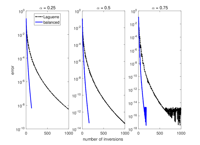
Figure 6. $\left\|\mathcal{L}^{-\alpha}-R_{{2j-1},2j}(\mathcal{L})\right\|$ vs the number of inversions $2j,$ for $j=n$ (Laguerre) and $j=k_{n}^{(1)}$ (balanced).

In Figure 7 we focus the attention on the truncated (balanced) approach. We plot the error and its estimate (48) with $C=1$ with respect to the number of inversions, that is, $2k_{n}^{(1)}.$ The results show the accuracy of the estimate.

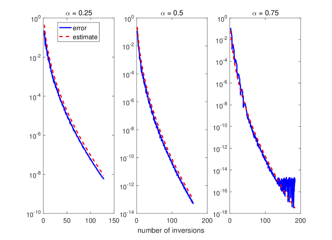
Figure 7. Error and its estimate given by (48) for the operator defined in (33).

When $\alpha>1/2$ the above estimate may be optimistic for $n\leq n^{\ast}$ (cf. (34)). Working with (35)-(38) with $S(n,\alpha)=g_{n}^{(2)}(1)$ and following the same analysis that starts from (44), by (30) we find that $k=2(1-\alpha)^{1/4}\left(2n/\pi\right)^{3/4}$ and then the value

(49) $$k_{n}^{(2)}:=2\left\lfloor(1-\alpha)^{1/4}\left(\frac{2n}{\pi}\right)^{3/4}\right\rfloor$$

is very close to $k_{n}.$ Therefore,

$$\left\|\mathcal{L}^{-\alpha}-R_{2k_{n}^{(2)}-1,2k_{n}^{(2)}}(\mathcal{L})\right\|\approx 4(1+C)\sin(\alpha\pi)$$

$$\times \exp\left(-2.96(1-\alpha)^{1/3}\left(2k_{n}^{(2)}\right)^{2/3}\right),\qquad\mbox{ for }\,(n\leq n^{\ast})\wedge(\alpha>1/2),$$

which expresses an initial convergence very fast with respect to the number of inversions. For $\alpha>1/2,$ one should use the first $k_{n}^{(2)}$ Laguerre points for $n\leq n^{\ast}$ and then switch to the first $k_{n}^{(1)}$ for $n>n^{\ast}.$ Anyway, experimentally it can be observe that the corresponding method does not offer a valuable improvement with respect to the choice of the first $k_{n}^{(1)},$ independently of $\alpha$ and $n$.

Therefore, the balanced approach that we propose is the one based on (46), and reported in the figures, with error estimate given by (48) independently of $\alpha$ and $n$.

6.2. An equalized approach

The idea is to work separately on the two integrals and hence to consider approximations of the type

$$\mathcal{L}^{-\alpha}\approx\frac{\sin(\alpha\pi)}{\alpha\pi}R_{k_{n_{1}}-1,k_{n_{1}}}^{(1)}(\mathcal{L})+\frac{\sin(\alpha\pi)}{(1-\alpha)\pi}R_{k_{n_{2}}-1,k_{n_{2}}}^{(2)}(\mathcal{L}),$$

in which $R_{k_{n_{i}}-1,k_{n_{i}}}^{(i)}(\lambda)$, $i=1,2$, represents the truncated Gauss-Laguerre rule for $I^{(i)}(\lambda)$ based on the first $k_{n_{i}}$ roots of the Laguerre polynomials of degree $n_{i}.$ For $n_{1}\neq n_{2}$ we use then different sets of points, and clearly the total number of inversions is now $k_{n_{1}}+k_{n_{2}}$.

We first consider the case where, for a given $n$, $\varepsilon_{n}^{(1)}({\lambda})/\alpha\geq\varepsilon_{n}^{(2)}(\lambda)/(1-\alpha)$ (cf. (15) and (16)) and we define $n_{1}=n$. Then, we evaluate $k_{n_{1}}=k_{n_{1}}^{(1)}$ as in (46) and we approximate $I^{(1)}(\mathcal{L})$ with $R_{k_{n_{1}}-1,k_{n_{1}}}^{(1)}(\mathcal{L})$. Then, we find $n_{2}$ ($\leq n_{1}$) such that

$$g_{n_{1}}^{(1)}({\lambda_{n_{1}}})=g_{n_{2}}^{(2)}(1)$$

that is,

(51) $$\exp\left(-3\left(n_{1}\alpha^{2}\pi^{2}\right)^{1/3}\right)=\exp\left(-\left(8\pi(1-\alpha)n_{2}\right)^{1/2}\right),$$

(cf. (29) and (30)). At this point we compute as in (49)

(52) $$k_{n_{2}}=k_{n_{2}}^{(2)}=2\left\lfloor(1-\alpha)^{1/4}\left(\frac{2n_{2}}{\pi}\right)^{3/4}\right\rfloor,$$

and use the Gauss-Laguerre rule $R_{k_{n_{2}}-1,k_{n_{2}}}^{(2)}(\mathcal{L})$ for the second integral. Clearly, for each $n$ the error estimate for the equalized approach remains the one of the balanced approach given by (48), but now we have less inversions. In this view, we have to find the relationship between $k_{n_{1}}$ and $k_{n_{2}}.$ From (51) we get

$$n_{2}=\frac{9}{8}\pi^{1/3}\frac{\alpha^{4/3}}{1-\alpha}n_{1}^{2/3}$$

so that using (52) we can express $k_{n_{2}}$ in terms of $n_{1}.$ Then, by (47) we obtain

$$k_{n_{2}}\approx\frac{3.09}{\alpha^{3/4}(1-\alpha)^{1/2}}k_{n_{1}}^{3/4}.$$

from which we deduce that $(k_{n_{1}}+k_{n_{2}})\leq 2k_{n_{1}}.$

As for the case $\varepsilon_{n}^{(1)}({\lambda})/\alpha<\varepsilon_{n}^{(2)}(\lambda)/(1-\alpha)$ the arguments follow the same line. Let $n_{2}=n$ and compute the second integral with $R_{k_{n_{2}}-1,k_{n_{2}}}^{(2)}(\mathcal{L})$. Then, solving (51) with respect to $n_{1}$ ($\leq n_{2}$) we obtain

$$n_{1}=\frac{\left(8(1-\alpha)\right)^{3/2}}{27\alpha^{2}\pi^{1/2}}n_{2}^{3/2}.$$

Consequently, as in (46)

$$k_{n_{1}}=k_{n_{1}}^{(1)}=\left\lfloor 2\sqrt{3}\left(\frac{\alpha n_{1}^{2}}{\pi^{2}}\right)^{1/3}\right\rfloor,$$

and we compute the first integral with $R_{k_{n_{1}}-1,k_{n_{1}}}^{(1)}(\mathcal{L})$. Using (49) we also have

$$k_{n_{2}}=2\left\lfloor(1-\alpha)^{1/4}\left(\frac{2n_{2}}{\pi}\right)^{3/4}\right\rfloor$$

and therefore, collecting the above expressions we finally obtain

$$k_{n_{1}}\approx 0.61\frac{(1-\alpha)^{2/3}}{\alpha}k_{n_{2}}^{4/3}.$$

As before, the error estimate for the equalized approach is the one of the balanced approach given by (6.1) but the number of inversions that we have to consider is now $(k_{n_{1}}+k_{n_{2}})\leq 2k_{n_{2}}$.

In Figure 8 we consider the comparison between our two truncated approaches together with Sinc rule analyzed in [7].

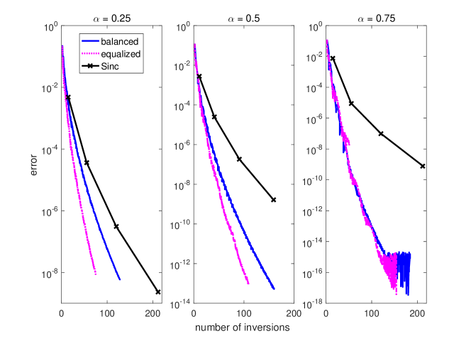
Figure 8. Comparison between the errors provided by the balanced and equalized approaches with the Sinc quadrature studied in [7].

7. Conclusions

In this work we have considered the construction of very fast methods based on the Gauss-Laguerre rule and we have been able to provide accurate error estimates that can be used to a priori select the number of points to use. We observe that while all the experiments concern the artificial example (33), other tests on finite difference discretizations of the Laplace operator have essentially led to identical results.

References

• [1] M. Abramowitz, I. Stegun. Handbook of Mathematical Functions with Formulas, Graphs, and Mathematical Tables. Dover Publications, Inc., New York, 1970
• [2] L. Aceto, P. Novati. Padé-type approximations to the resolvent of fractional powers of operators. J. Sci. Comput. 83 (2020): 13, DOI:10.1007/s10915-020-01198-w, in press
• [3] L. Aceto, P. Novati. Rational approximations to fractional powers of self-adjoint positive operators. Numer. Math. 143, 1-16 (2019)
• [4] L. Aceto, D. Bertaccini, F. Durastante, P. Novati. Rational Krylov methods for functions of matrices with applications to fractional partial differential equations. J. Comput. Phys. 396, 470-482 (2019)
• [5] W. Barrett. Convergence properties of Gaussian quadrature formulae. Comput. J. 3(4), 272-277 (1961)
• [6] B. S. Berger. Dynamic response of an infinite cylindrical shell in acoustic medium. J. Appl. Mech. 36, 342-345 (1969)
• [7] A. Bonito, J.E. Pasciak. Numerical approximation of fractional powers of elliptic operators. Math. Comp. 84, 2083-2110 (2015)
• [8] P.J. Davis, P. Rabinowitz. Methods of Numerical Integration. Academic Press, 1984
• [9] D. Elliott. Truncation errors in Padé approximations to certain functions: an alternative approach. Math. Comp. 21, 398-406 (1967)
• [10] S. Harizanov, R. Lazarov, S. Margenov, P. Marinov, Y. Vutov. Optimal solvers for linear systems with fractional powers of sparse SPD matrices. Numer. Linear Algebra Appl. 25(5), e2167 (2018)
• [11] S. Harizanov, R. Lazarov, P. Marinov, S. Margenov, J.E. Pasciak. Analysis of numerical methods for spectral fractional elliptic equations based on the best uniform rational approximation. arXiv:1905.08155v2 (2019)
• [12] S. Harizanov, R. Lazarov, P. Marinov, S. Margenov, J.E. Pasciak. Comparison analysis of two numerical methods for fractional diffusion problems based on the best rational approximations of $t^{\gamma}$ on $[0,1].$ In: Apel T., Langer U., Meyer A., Steinbach O. (eds) Advanced Finite Element Methods with Applications. FEM 2017. Lecture Notes in Computational Science and Engineering, vol 128. Springer, Cham, 2019
• [13] S. Harizanov, S. Margenov. Positive approximations of the inverse of fractional powers of SPD M-Matrices. In: Feichtinger G., Kovacevic R., Tragler G. (eds) Control Systems and Mathematical Methods in Economics. Lecture Notes in Economics and Mathematical Systems, vol 687. Springer, Cham, 2018
• [14] C. Hofreither. A unified view of some numerical methods for fractional diffusion. Comput. Math. Appl. (2019), DOI: 10.1016/j.camwa.2019.07.025, in press
• [15] G. Mastroianni, G. Monegato. Truncated quadrature rules over and Nystrom-type methods. SIAM J. Numer. Anal. 41, 1870-1892 (2004)
• [16] G. Mastroianni, D. Occorsio. Lagrange interpolation at Laguerre zeros in some weighted uniform spaces. Acta Math. Hungar. 91(1–2), 27-52 (2001)
• [17] L.J. Slater. Confluent Hypergeometric Functions. Cambridge University Press, Cambridge, 1960
• [18] H.R. Stahl. Best uniform rational approximation of $x^{\alpha}$ on $[0,1].$ Acta Math. 190, 241-306 (2003)
• [19] G. Szegö. Orthogonal Polynomials. American Mathematical Society. Providence, Rhode Island, 1939
• [20] P.N. Vabishchevich. Approximation of a fractional power of an elliptic operator. CoRR abs/1905.10838 (2019)
• [21] P.N. Vabishchevich. Numerical solution of time-dependent problems with fractional power elliptic operator. Comput. Meth. in Appl. Math. 18(1), 111-128 (2018)
• [22] P.N. Vabishchevich. Numerically solving an equation for fractional powers of elliptic operators. J. Comput. Phys. 282, 289-302 (2015)
• [23] G. Van Damme. Legendre Laguerre and Hermite - Gauss Quadrature (https://www.mathworks.com/matlabcentral/fileexchange/26737-legendre-laguerre-and-hermite-gauss-quadrature), MATLAB Central File Exchange, 2020.