Universal Quantization of Magnetic Susceptibility Jump at Topological Phase Transition

Abstract

We examine the magnetic susceptibility of topological insulators microscopically and find that the orbital–Zeeman (OZ) cross term, the cross term between the orbital effect and the spin Zeeman effect, is directly related to the Berry curvature when the $z$-component of spin is conserved. In particular, the OZ cross term reflects the spin Chern number, which results in the quantization of the magnetic susceptibility jump at the topological phase transition. The magnitude of the jump is in units of the universal value $4|e|\mu_{\rm B}/h$. The physical origin of this quantization is clarified. We also apply the obtained formula to an explicit model and demonstrate the quantization.

Introduction.—Topological insulators (TIs) Kane and Mele (2005a, b); Bernevig and Zhang (2006); Bernevig et al. (2006); M.-F. Yang and M.-C. Chang (2006); Murakami (2006); M. König et al. (2007); A.Roth et al. (2009); C. Brüne et al. (2012); Knez et al. (2011, 2012); Fu and Kane (2007); Hsieh et al. (2008) show anomalous phenomena such as electric conduction on sample surfaces. Experimentally, the search for candidate materials for TIs is one of the most important problems. In particular, two-dimensional (2D) TIs are predicted to show unique phenomena, such as the spin Hall effect and robust edge states against nonmagnetic impurities, only a few of which have been found M. König et al. (2007); A.Roth et al. (2009); C. Brüne et al. (2012); Knez et al. (2011, 2012). So far, the confirmation of topological materials has been achieved by finding the edge state by angle-resolved photoemission spectroscopy or from the transport coefficients. Since both methods detect anomalous electronic states at the edge, it is desirable to develop some bulk-sensitive methods that enable us to confirm the topological nature of a material. In this Letter, we propose that the quantization of the bulk magnetic susceptibility jump can be used as strong evidence for the topological phase transition in 2D TIs.

Usually, the magnetic susceptibility is discussed in terms of the orbital effect of the magnetic field Landau (1930); Peierls (1933); Hebborn and Sondheimer (1960); Blount (1962); Hebborn et al. (1964); Wannier and Upadhyaya (1964); Fukuyama (1971); Fukuyama and Kubo (1970); Ogata and Fukuyama (2015); McClure (1956); Fukuyama (2007); G. Gómez-Santos and Stauber (2011); Koshino and Ando (2010); Ogata (2016); Gao et al. (2015); Raoux et al. (2015); Piéchon et al. (2016) and spin Zeeman effect independently. In general, however, there can be a cross term between the orbital and Zeeman effects M.-F. Yang and M.-C. Chang (2006); Murakami (2006); Ito and Nomura (2017); Tserkovnyak et al. (2015); Koshino and Hizbullah (2016); Nakai and Nomura (2016); Ogata (2017), which we call the orbital–Zeeman (OZ) cross term $\chi_{\rm OZ}$ in the following. Recently, Nakai and Nomura Nakai and Nomura (2016) discussed the jump in $\chi_{\rm OZ}$ at the topological phase transition using the formula of the orbital magnetization Xiao et al. (2010); Thonhauser (2011); Sundaram and Niu (1999); Xiao et al. (2005); Thonhauser et al. (2005); Ceresoli et al. (2006); Shi et al. (2007) and the Středa formula P. Středa (1982). They calculated the OZ cross term in the Bernevig–Hughes–Zhang model Bernevig et al. (2006) and concluded that the width of the jump depends on the $g$-factors of the involved orbitals introduced phenomenologically. In general, spin–orbit interaction (SOI) modifies the $g$-factor from its bare value $g_{0}=2$. (Here, we neglect the relativistic correction of $g_{0}$.) Thus, their conclusion means that the jump in $\chi_{\rm OZ}$ is not quantized in a universal value.

In the present Letter, we study $\chi_{\rm OZ}$ microscopically based on the Green’s function formalism and show that, in contrast to the results of Nakai and Nomura, the jump in $\chi_{\rm OZ}$ is exactly quantized in units of the universal value $4|e|\mu_{\rm B}/h$ (see Eq. (8) below) even in the presence of SOI as long as the $z$-component of the spin is conserved. Here, $\mu_{\rm B}=|e|\hbar/2m$ is the Bohr magneton. When we study a model microscopically (as in Eq. (1)), the modification of the $g$-factor does not occur explicitly, and instead the effect of SOI appears in the deformation of the Bloch wave functions and the energy dispersion, which eventually leads to the orbital-dependent $g$-factors. We show below that the effect of SOI is exactly cancelled out in $\chi_{\rm OZ}$, which leads to the quantization of jump with a universal value. We also clarify the physical origin of this result: it turns out that the quantization is associated with the chiral edge current, which is characteristic of the topological nontrivial state. Finally, we apply the obtained formula to Kane–Mele model Kane and Mele (2005b, a) to show the validity of the present proposal.

General formalism.—First, we develop microscopically a general formula for magnetic susceptibility including orbital magnetism, Pauli paramagnetism, and the OZ cross term in terms of thermal Green’s functions in the presence of SOI. Let $H$ be the general Hamiltonian derived from the Dirac equation in the presence of a periodic potential $V(\bm{r})$ and a magnetic field, which is given by

$$H= \frac{1}{2m}({\bm{p}}-e{\bm{A}(\bm{r})})^{2}-\frac{e\hbar}{2m}\bm{\sigma}\cdot{\bm{B}(\bm{r})}+V({\bm{r}})$$

$$+\frac{\hbar^{2}}{8m^{2}c^{2}}\nabla^{2}V+\frac{\hbar}{4m^{2}c^{2}}\bm{\sigma}\cdot\nabla V\times({\bm{p}}-e{\bm{A}(\bm{r})}),$$ (1)

where ${\bm{A}(\bm{r})}$ is a vector potential, $e<0$ for electrons, $\bm{\sigma}=(\sigma_{x},\sigma_{y}.\sigma_{z})$ are $2\times 2$ Pauli matrices, and ${\bm{B}(\bm{r})}=\nabla\times{\bm{A}(\bm{r})}$ represents a magnetic field. The last term represents the SOI. It is to be noted that the second term representing the Zeeman interaction has the bare value $g_{0}=2$. As performed by Fukuyama Fukuyama (1971), we implement a perturbative calculation of the free energy in terms of the vector potential $\bm{A}(\bm{r})$ via the Luttinger–Kohn representation Luttinger and Kohn (1955). As a result, we obtain the expression for each contribution as follows (The details of the derivation are shown in the Supplemental Material (SM) sm .):

$$\chi_{\rm orbit}=\frac{e^{2}}{2\hbar^{2}}\frac{k_{\rm B}T}{V}\sum_{n{\bm{k}}}{\rm Tr}\,\gamma_{x}\mathcal{G}\gamma_{y}\mathcal{G}\gamma_{x}\mathcal{G}\gamma_{y}\mathcal{G},$$ (2a)

$$\chi_{\rm Pauli}=-\frac{k_{\rm B}T}{V}\sum_{n{\bm{k}}}{\rm Tr}\,M_{z}^{s}\mathcal{G}M_{z}^{s}\mathcal{G},$$ (2b)

$$\chi_{\rm OZ}=-\frac{i|e|}{\hbar}\frac{k_{\rm B}T}{V}\sum_{n{\bm{k}}}{\rm Tr}[M_{z}^{s}\mathcal{G}\gamma_{x}\mathcal{G}\gamma_{y}\mathcal{G}-M_{z}^{s}\mathcal{G}\gamma_{y}\mathcal{G}\gamma_{x}\mathcal{G}],$$ (2c)

where $\mathcal{G}$ is the thermal Green’s function $\mathcal{G}({\bm{k}},i\varepsilon_{n})$, whose $(ll^{\prime})$ component is the matrix element between the $l$th and $l^{\prime}$th bands. Each band index includes the pseudo-spin degrees of freedom in the case with SOI. $\varepsilon_{n}$ is the Matsubara frequency, $\gamma_{\mu}$ represents the current operator in the $\mu$-direction divided by $e/\hbar$, and $M_{z}^{s}$ is the matrix for the operator $-\mu_{\rm B}\sigma_{z}$. The effect of SOI is included in $\mathcal{G}$ and $\gamma_{\mu}$. Tr is the trace over the band indices and the spin degrees of freedom. In Eq. (2), $\chi_{\rm orbit}$ and $\chi_{\rm Pauli}$ respresent the orbital and Pauli magnetic susceptibility, respectively. These are the same expressions as were obtained before Fukuyama (1971); Okuma and Ogata (2015) even in the presence of SOI. On the other hand, $\chi_{\rm OZ}$ is the OZ cross term, which we focus on in this Letter.

To discuss the quantization, we rewrite Eq. (2c) in terms of the Bloch wave functions in a similar way to Ref. Ogata and Fukuyama (2015). The periodic part of the Bloch wave function $\hat{u}_{l{\bm{k}}}$ satisfies

$$H_{\bm{k}}\hat{u}_{l{\bm{k}}}(\bm{r})=\varepsilon_{l}(\bm{k})\hat{u}_{l{\bm{k}}}(\bm{r}),$$ (3)

where $H_{{\bm{k}}}=e^{-i{\bm{k}}\bm{r}}He^{i{\bm{k}}\bm{r}}$ and $\hat{u}_{l{\bm{k}}}(\bm{r})$ is a 2-component vector $\hat{u}_{l{\bm{k}}}({\bm{r}})=\,^{t}(u_{l{\bm{k}}\uparrow}(\bm{r}),u_{l{\bm{k}}\downarrow}(\bm{r}))$ in the presence of SOI. In the following, we consider the case where the $z$-component of spin is conserved even in the presence of SOI. In this case, up- and down-spin electrons are independent, and the energy dispersion is $\varepsilon_{l\sigma}({\bm{k}})$ (denoted as $\varepsilon_{l\sigma}$ in the following). The matrices $\mathcal{G}$ and $M_{z}^{s}$ are diagonal and given by $[\mathcal{G}_{\sigma}]_{ll^{\prime}}=\delta_{ll^{\prime}}(i\varepsilon_{n}-\varepsilon_{l\sigma}+\mu)^{-1}$ and $[M^{s}_{z\sigma}]_{ll^{\prime}}=-\sigma\mu_{\rm B}\delta_{ll^{\prime}}$, respectively. On the other hand, the matrix $\gamma_{\mu}$ has off-diagonal matrix elements between the different bands and it becomes,

$$[\gamma_{\mu\sigma}]_{ll^{\prime}} =\int u^{*}_{l{\bm{k}}\sigma}\frac{\partial H_{\bm{k}}}{\partial k_{\mu}}u_{l^{\prime}{\bm{k}}\sigma}d{\bm{r}},$$

$$=\frac{\partial\varepsilon_{l\sigma}}{\partial k_{\mu}}\delta_{ll^{\prime}}+(\varepsilon_{l^{\prime}\sigma}-\varepsilon_{l\sigma})\int u_{l{\bm{k}}\sigma}^{*}\frac{\partial u_{l^{\prime}{\bm{k}}\sigma}}{\partial k_{\mu}}d{\bm{r}}.$$ (4)

where $u_{l{\bm{k}}\sigma}$ is the abbreviation for $u_{l{\bm{k}}\sigma}(\bm{r})$. Substituting these quantities into Eq. (2c) and carrying out the Matsubara summation, we obtain

$$\chi_{\rm OZ}=-\frac{2|e|\mu_{\rm B}}{\hbar V}\sum_{l{\bm{k}}\sigma}f(\varepsilon_{l\sigma})\sigma\Omega_{l{\bm{k}}\sigma}^{z}+\frac{i|e|\mu_{\rm B}}{\hbar V}\sum_{l{\bm{k}}\sigma}\sigma f^{\prime}(\varepsilon_{l})\left\{\int\frac{\partial u^{*}_{l{\bm{k}}\sigma}}{\partial k_{x}}(\varepsilon_{l\sigma}-H_{\bm{k}})\frac{\partial u_{l{\bm{k}}\sigma}}{\partial k_{y}}d{\bm{r}}-(x\leftrightarrow y)\right\}\;,$$ (5)

where $\Omega_{l\sigma}^{z}$ is the Berry curvature in the $z$-direction,

$$\Omega_{l{\bm{k}}\sigma}^{z}=i\int\left(\frac{\partial u^{*}_{l{\bm{k}}\sigma}}{\partial k_{x}}\frac{\partial u_{l{\bm{k}}\sigma}}{\partial k_{y}}-\frac{\partial u^{*}_{l{\bm{k}}\sigma}}{\partial k_{y}}\frac{\partial u_{l{\bm{k}}\sigma}}{\partial k_{x}}\right)d{\bm{r}},$$ (6)

$f(\varepsilon)=(1+e^{(\varepsilon-\mu)/k_{\rm B}T})^{-1}$, and the completeness condition $\sum_{l^{\prime}\sigma}u_{l^{\prime}{\bm{k}}\sigma}(\bm{r})u_{l^{\prime}{\bm{k}}\sigma}^{*}(\bm{r}^{\prime})=\delta(\bm{r}-\bm{r}^{\prime})$ has been used to take the summation over the intermediate state $l^{\prime}$.

Universal quantization of $\chi_{\rm OZ}$.—Let us consider $\chi_{\rm OZ}$ in TIs. The second term in Eq. (5) does not contribute in insulators at zero temperature because the Fermi surface is absent. Then $\chi_{\rm OZ}$ is written as

$$\chi_{\rm OZ}=-\frac{2|e|\mu_{\rm B}}{\hbar V}\sum_{l:{\rm occ}}\sum_{{\bm{k}}\sigma}\sigma\Omega^{z}_{l{\bm{k}}\sigma},$$ (7)

where the summation $\sum_{l:{\rm occ}}$ is taken for the occupied bands. Furthermore, in the case of a 2D insulator, we obtain

$$\chi_{\rm OZ}^{\rm 2D}=-\frac{4|e|\mu_{\rm B}}{h}\sum_{l:{\rm occ}}{\rm Ch}_{{\rm s},l},$$ (8)

where ${\rm Ch}_{{\rm s},l}$ is the spin Chern number for the $l$th band defined by

$${\rm Ch}_{{\rm s},l}=\frac{1}{2}\frac{2\pi}{L^{2}}\sum_{\bm{k}}(\Omega_{l{\bm{k}}\uparrow}-\Omega_{l{\bm{k}}\downarrow}).$$ (9)

At a topological phase transition, ${\rm Ch}_{{\rm s},l}$ changes from one integer to another. Therefore, Eq. (8) leads to the quantization of the magnetic susceptibility jump at the topological phase transition. The magnitude of the jump is in units of $\chi_{0}=4|e|\mu_{\rm B}/h$, which is universal. Although the effect of SOI is included in $u_{l{\bm{k}}\sigma}$, it does not affect the coefficient in Eq. (8) since ${\rm Ch}_{{\rm s},l}$ is a topological number, which leads to the universal quantization of jump in $\chi_{\rm OZ}$.

Physical origin of quantization.—Let us consider the physical origin of this quantization. $\chi_{\rm OZ}$ is interpreted as the sum of the correction to the orbital magnetic moment induced by the magnetic field that couples to the spin magnetic moment and the correction to the spin magnetic moment induced by the magnetic field that couples to the orbital magnetic moment. Here, we estimate the former correction. In the edge state, there are spin-polarized linear dispersions and a spin current flows. Figure 1(a) corresponds to the state with ${\rm Ch}_{{\rm s},l}=+1$. (Note that the number of pairs of dispersion coincides with $|{\rm Ch}_{{\rm s},l}|$.) When a magnetic field is applied through the Zeeman interaction $\mu_{\rm B}\sigma_{z}B$, the up-spin (down-spin) band moves upward (downward) as shown in Fig. 1(b). The width of change $\Delta$ is $\mu_{\rm B}B$. Then, in the lowest energy state [Fig. 1(c)], the number of down-spin (up-spin) electrons increases (decreases) by $\nu\mu_{\rm B}B$, where $\nu$ is the density of states $\nu=L/ch$ and $c$ is the velocity of the edge current. This change leads to an electric current of $-2|e|\mu_{\rm B}B/h$ in the right direction, which causes the orbital magnetic moment of $-2|e|\mu_{\rm B}B/h$ per area. The coefficient of $B$ is half of the quantization of magnetic susceptibility, $-\chi_{0}/2$. We can also estimate the contribution from the other correction (i.e., the spin magnetic moment induced by an energy shift originating from an orbital magnetic moment made by a circular electric current), which gives the same value. Combining these two contributions, we obtain the OZ cross term as $-\chi_{0}$, which is consistent with Eq. (8).

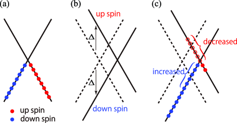
Figure 1: Schematic pictures for the edge state. (a) Ground state without an external magnetic field. (b) Change caused by the Zeeman interaction. (c) New ground state in the magnetic field.

Explicit calculation of $\chi_{\rm OZ}$ in Kane–Mele model.—In the rest of this Letter, we calculate the magnetic susceptibility of a model for a 2D TI to show that $\chi_{\rm OZ}$ actually has a jump at the topological phase transition and that other contributions do not conceal the quantized jump. We introduce the Kane–Mele model Kane and Mele (2005a, b); Guzmán-Verri and Voon (2007); C.-C. Liu et al. (2011a); Ezawa (2012a, b); C.-C. Liu et al. (2011b),

$$H=- \sum_{\langle i,j\rangle\alpha}tc_{i\alpha}^{\dagger}c_{j\alpha}+\Delta_{0}\left(\sum_{i\in{\rm A},\alpha}c_{i\alpha}^{\dagger}c_{i\alpha}-\sum_{i\in{\rm B},\alpha}c_{i\alpha}^{\dagger}c_{i\alpha}\right)$$

$$+\sum_{\langle\langle i,j\rangle\rangle,\alpha\beta}it_{2}\nu_{ij}c_{i\alpha}^{\dagger}s_{\alpha\beta}^{z}c_{j\beta},$$ (10)

where $c^{\dagger}_{i\alpha}$ is the creation operator of an electron with spin $\alpha$ at site $i$, and the summation $\langle i,j\rangle$ ($\langle\langle i,j\rangle\rangle$) runs over all the nearest- (next-nearest-) neighbor sites of the 2D honeycomb lattice. The first term represents the usual nearest-neighbor hopping with transfer integral $t$. The second term represents a staggered on-site potential, $+\Delta_{0}$ for A sublattice and $-\Delta_{0}$ for B sublattice. The last term represents the hopping originating from SOI. We take account of only the $s^{z}$-component as in Ref. Kane and Mele (2005b) and set $\nu_{ij}=-\nu_{ji}=+1\,(-1)$ if the electron makes a left (right) turn to propagate to the next-nearest sites. This model is known as one for silicene Guzmán-Verri and Voon (2007); C.-C. Liu et al. (2011a); Ezawa (2012a, b); C.-C. Liu et al. (2011b). We can control $\Delta_{0}$ by changing the electric field applied perpendicular to the layer due to its buckled structure.

The energy dispersion of this model is shown in Fig. 2 for case (a) with $\Delta_{0}/t=1/4,t_{2}/t=\sqrt{3}/36$ (topologically trivial; solid line) and for case (b) with $\Delta_{0}/t=1/4,t_{2}/t=\sqrt{3}/12$ (topologically nontrivial; dashed line). In the following, we use (a) and (b) as typical cases. The explicit expression of the energy dispersion is shown in SM sm . Since the space inversion symmetry is broken, the energy dispersions for up and down spins can be different. In the momentum space, gaps open at $K=(4\pi/3\sqrt{3}a,0)$ and $K^{\prime}=(-4\pi/3\sqrt{3}a,0)$ with $a$ being the distance between the nearest-neighbor sites. Their magnitudes are $2\left|\Delta_{0}+(3\sqrt{3}/2)\sigma t_{2}\right|$ at $K$ and $2\left|\Delta_{0}-(3\sqrt{3}/2)\sigma t_{2}\right|$ at $K^{\prime}$, respectively, where $\sigma=1$ is for up spin and $\sigma=-1$ is for down spin.

In this model, the ratio of $\Delta_{0}$ to $t_{2}$ determines the topological order C.-C. Liu et al. (2011b); Ezawa (2012a, b): topologically trivial for $|t_{2}/\Delta_{0}|<2/3\sqrt{3}$ and topologically nontrivial for $|t_{2}/\Delta_{0}|>2/3\sqrt{3}$. The phase diagram is shown in the inset of Fig. 2.

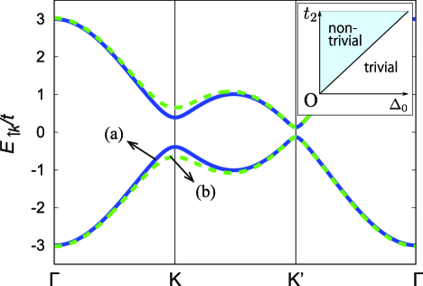
Figure 2: Energy dispersion for $\sigma=1$ (up spin) of the model in Eq. (10) along the path $\Gamma\rightarrow K\rightarrow K^{\prime}\rightarrow\Gamma$ for two typical choices of parameters: (a) solid line, $\Delta_{0}/t=1/4,t_{2}/t=\sqrt{3}/36$ (topologically trivial) and (b) dashed line, $\Delta_{0}/t=1/4,t_{2}/t=\sqrt{3}/12$ (topologically nontrivial). The energy dispersion for $\sigma=-1$ (down spin) is obtained by exchanging $K$ for $K^{\prime}$ points. Inset: Phase diagram of this model.

Before calculating magnetic susceptibility, let us examine the Berry curvature. Figure 3 shows the distribution of the Berry curvature in the momentum space for the valence band electrons with up spin for the two choices of the parameters in Fig. 2. It is seen that the Berry curvature is localized near $K$ and $K^{\prime}$ points. After numerical integration, we find that the Chern numbers are $0$ for (a) and $1$ for (b), which is consistent with the fact that cases (a) and (b) belong to the topologically trivial and nontrivial phases, respectively.

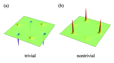
Figure 3: Distribution of Berry curvature in the momentum space for the valence band electrons with up spin for case of (a) (topologically trivial) and (b) (topologically nontrivial). The Chern numbers are $0$ for (a) and $1$ for (b).

According to Figs. 2 and 3, the low-energy excitations in the vicinity of $K$ and $K^{\prime}$ points are important when $\mu\simeq 0$. Therefore, we approximate the Hamiltonian by the expansion around $K$ and $K^{\prime}$ points, i.e., $\bm{k}\cdot\bm{p}$ perturbation. In this way, we obtain a low-energy effective model,

$$h^{K/K^{\prime}}_{\sigma}=(\Delta^{K/K^{\prime}}_{\sigma}-\sigma\alpha k^{2})\tau_{z}+\hbar v_{\rm F}k_{x}\tau_{x}+\hbar v_{\rm F}k_{y}\tau_{y},$$ (11)

where $\tau_{x}$, $\tau_{y}$, and $\tau_{z}$ are the Pauli matrices representing the degrees of freedom of sublattices A and B, $\Delta^{K}_{\sigma}=\Delta_{0}+\sigma(3\sqrt{3}/2)t_{2}$, $\Delta^{K^{\prime}}_{\sigma}=-\Delta_{0}+\sigma(3\sqrt{3}/2)t_{2}$, $\alpha=(9\sqrt{3}/8)a^{2}t_{2}$, and $\hbar v_{\rm F}=(3/2)at$. Note that the signs of the mass term $\Delta_{\sigma}^{K/K^{\prime}}$ at $K$ and $K^{\prime}$ points with different spins are opposite, i.e., $\Delta^{K}_{\uparrow}=-\Delta^{K^{\prime}}_{\downarrow}$ and $\Delta^{K}_{\downarrow}=-\Delta^{K^{\prime}}_{\uparrow}$. This effective Hamiltonian is justified in the limit of $t_{2},\Delta_{0}\rightarrow 0$ with $t_{2}/\Delta_{0}$ fixed.

Let us discuss the magnetic susceptibility. Note that Ezawa Ezawa (2012b) calculated the orbital magnetism but the OZ cross term was not taken into account. In the model Eq. (11), the thermal Green’s function is defined as $\mathcal{G}_{\sigma}^{K/K^{\prime}}=(i\varepsilon_{n}-h^{K/K^{\prime}}_{\sigma})^{-1}$. The current operator in the $\mu$-direction is given by $\gamma_{\mu}=\hbar v_{\rm F}\tau_{\mu}-2\sigma\alpha k_{\mu}\tau_{z}$. Substituting these quantities into Eq. (2), carrying out the Matsubara summation, and performing the 2D momentum integration at $T=0$, we obtain

$$\chi_{\rm orbit}=-\frac{e^{2}v_{\rm F}^{2}}{6\pi}\sum_{\eta=K,K^{\prime}}\frac{1}{|\Delta_{\uparrow}^{\eta}|}\theta(|\Delta_{\uparrow}^{\eta}|-|\mu|),$$ (12a)

$$\chi_{\rm Pauli}=\frac{\mu_{\rm B}^{2}}{\pi\hbar^{2}v_{\rm F}^{2}}\sum_{\eta=K,K^{\prime}}|\mu|\theta(|\mu|-|\Delta_{\uparrow}^{\eta}|),$$ (12b)

$$\chi_{\rm OZ}=-\frac{2\mu_{\rm B}|e|}{h}\sum_{\eta=K,K^{\prime}}{\rm sgn}(\Delta_{\uparrow}^{\eta})\theta(|\Delta_{\uparrow}^{\eta}|-|\mu|),$$ (12c)

in the limit of $t_{2},\Delta_{0}\rightarrow 0$ with $t_{2}/\Delta_{0}$ fixed. Here, $\chi_{\rm orbit}$ is the orbital diamagnetic susceptibility of the 2D Dirac electrons discussed in the preceding studies McClure (1956); Fukuyama (2007); G. Gómez-Santos and Stauber (2011); Ogata (2016); Koshino and Ando (2010); Gao et al. (2015); Raoux et al. (2015). $\chi_{\rm Pauli}$ is the Pauli paramagnetism proportional to the density of states ($\propto|\mu|$).

To observe the quantization of the jump, we focus on the case of $\mu=0$, an insulating case, where $\chi_{\rm Pauli}$ vanishes. Figure 4 shows $\chi_{\rm orbit}$ and $\chi_{\rm OZ}$ as a function of $t_{2}/\Delta_{0}$. When $(3\sqrt{3}/2)t_{2}/\Delta_{0}<1$, the system is topologically trivial and the signs of $\Delta_{\uparrow}^{K}$ and $\Delta_{\uparrow}^{K^{\prime}}$ are opposite, which leads to $\chi_{\rm OZ}=0$ from Eq. (12c). When $(3\sqrt{3}/2)t_{2}/\Delta_{0}>1$, on the other hand, the system is topologically nontrivial and the signs of $\Delta_{\uparrow}^{K}$ and $\Delta_{\uparrow}^{K^{\prime}}$ are the same, which leads to $\chi_{\rm OZ}=-\chi_{0}$. As a result, $\chi_{\rm OZ}$ has a universal jump at the topological phase transition at $t_{2}/\Delta_{0}=2/3\sqrt{3}$. On the other hand, $\chi_{\rm orbit}$ diverges at the phase transition due to the gap closing. However, we can see that $\chi_{\rm orbit}=-\frac{e^{2}v_{\rm F}^{2}}{6\pi}(|\Delta_{0}-3\sqrt{3}t_{2}/2|^{-1}+|\Delta_{0}+3\sqrt{3}t_{2}/2|^{-1})$ and the magnitude of divergence is the same on both sides of the phase transition. Therefore, when we subtract the divergence of $\chi_{\rm orbit}$, we will be able to detect the jump in $\chi_{\rm OZ}$. Note that the effect of SOI represented by $t_{2}$ appears only in the magnitude of $\chi_{\rm orbit}$ and does not affect the magnitude of $\chi_{\rm OZ}$.

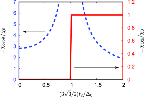
Figure 4: Contributions to magnetic susceptibility as a function of $(3\sqrt{3}/2)t_{2}/\Delta_{0}$ for $\mu=0$ with $\Delta_{0}=t/4$. They are normalized by $\chi_{0}$. The values of $v_{\rm F}$ and $a$ are chosen to be the same as those of graphene. The system is topologically trivial (nontrivial) in the region $(3\sqrt{3}/2)t_{2}/\Delta_{0}<1(>1)$.

Discussion and conclusion.—The expression for the magnetic susceptibility including the spin Zeeman effect was obtained in terms of Bloch wave functions Ogata (2017), which contains a term $\chi_{\rm occ:2}=-\frac{e}{\hbar}{\rm Re}\sum_{l{\bm{k}}}f(\varepsilon_{\bm{k}})M_{ll}^{z}\Omega_{l}^{z}.$ Actually, $\chi_{\rm occ:2}$ gives half of $\chi_{\rm OZ}$ in Eq. (8). The origin of this difference is as follows. In Ref. Ogata (2017), the effect of Zeeman interaction is distributed among several terms for total magnetic susceptibility including $\chi_{\rm occ:2}$. Therefore, if we collect all the effects of Zeeman interaction in the formalism of Ref. Ogata (2017), we can recover $\chi_{\rm OZ}$.

Based on the microscopic theory, we have derived a new simple formula for magnetic susceptibility in a Bloch system with SOI and Zeeman interaction to show that the OZ cross term, one of the three contributions to magnetic susceptibility, is always quantized in units of the universal value $4|e|\mu_{\rm B}/h$ for 2D spin-conserving insulators at zero temperature. We have clarified that this quantization originates from the redistribution of the chiral edge state due to the magnetic field. We have also applied the formula to a model for a 2D TI and demonstrated the quantization. Our results clearly show that the magnetic response reflects the topological nature of a material. It should be possible, therefore, to make a bulk-sensitive confirmation of the topological phase transition.