Superconductivity in Cu-doped Bi₂Se₃ with potential disorder

Abstract

We study the effects of random nonmagnetic impurities on superconducting transition temperature $T_{c}$ in a Cu-doped Bi₂Se₃, for which four types of pair potentials have been proposed. Although all the candidates belong to $s$-wave symmetry, two orbital degree of freedom in electronic structures enriches the symmetry variety of a Cooper pair such as even-orbital-parity and odd-orbital-parity. We consider realistic electronic structures of Cu-doped Bi₂Se₃ by using tight-binding Hamiltonian on a hexagonal lattice and consider effects of impurity scatterings through the self-energy of the Green’s function within the Born approximation. We find that even-orbital-parity spin-singlet superconductivity is basically robust even in the presence of impurities. The degree of the robustness depends on the electronic structures in the normal state and on the pairing symmetry in orbital space. On the other hand, two odd-orbital-parity spin-triplet order parameters are always fragile in the presence of potential disorder.

I Introduction

The robustness of superconductivity in the presence of nonmagnetic impurities depends on symmetry of the pair potential. The transition temperature $T_{c}$ is insensitive to the impurity concentration in a spin-singlet $s$-wave superconductor Abrikosov et al. (1975); Abrikosov and Gor’kov (1959); Anderson (1959). In a cuprate superconductor, on the other hand, $T_{c}$ of a spin-singlet $d$-wave superconductivity is suppressed drastically by the impurity scatterings Sun and Maki (1995). The pair potential of an unconventional superconductor changes its sign on the Fermi surface depending on the direction of a quasiparticle’s momenta. The random impurity scatterings make the motion of a quasiparticle be isotropic in both real and momentum spaces. Such a diffused quasiparticle feels the pair potential averaged over the directions of momenta. The resulting pair potential is finite for an $s$-wave symmetry, whereas it is zero for unconventional pairing symmetries. Thus, unconventional superconductivity is fragile under the potential disorder.

Previous papers Allen and Mitrovic (1983); Golubov and Mazin (1997); Efremov et al. (2011); Asano and Golubov (2018); Asano et al. (2018) showed that $s$-wave superconductivity is not always robust against the nonmagnetic impurity scatterings in multiband (multiorbital) superconductors. The interorbital impurity scatterings decrease $T_{c}$, which is a common conclusion of all the theoretical studies. The two-band models considered in these papers, however, are too simple to discuss the effects of impurities on $T_{c}$ in real materials such as iron pnictides Kamihara et al. (2008); Kuroki et al. (2008), MgB₂ Nagamatsu et al. (2001); Choi et al. (2002), and Cu-doped Bi₂Se₃ Hor et al. (2010); Fu and Berg (2010). The robustness of multiband superconductivity under the potential disorder may depend on electronic structures near the Fermi level. In iron pnictides and MgB₂, two electrons in the same conduction band form a Cooper pair Kuroki et al. (2008); Choi et al. (2002). The impurity effect on such an intraband pair has been studied by taking realistic electronic structures into account Onari and Kontani (2009). In the case of Cu-doped Bi₂Se₃, four types of pair potentials $\Delta_{1}-\Delta_{4}$ have been proposed as a promising candidate of order parameter Fu and Berg (2010). Among them, an interorbital pairing order has attracted much attention as a topologically nontrivial superconductivity Fu and Berg (2010); Sasaki et al. (2011). Unfortunately, the possibility of such a topological superconductivity under the potential disorder has never been studied yet. We address this issue.

In this paper, we study the effects of impurities on $T_{c}$ of Cu-doped Bi₂Se₃. We describe electronic structures near the Fermi level by taking into account two $p$ orbitals in Bi₂Se₃ and the hybridization between them Zhang et al. (2009); Liu et al. (2010). According to the theoretical proposal Fu and Berg (2010), we consider four types of $s$-wave pair potential on such orbital based electronic structures. The effects of impurities on $T_{c}$ are estimated through the impurity self-energy within the Born approximation. The transition temperature is calculated by solving the gap equation numerically and is plotted as a function of impurity concentration $n_{\mathrm{imp}}$. We will show that the relation between $T_{c}$ and $n_{\mathrm{imp}}$ depends sensitively on the types of pair potentials. Superconductivity with an intraorbital pair potential $\Delta_{1}$ is robust even in the dirty regime. This conclusion is consistent with that at a limiting case of previous studies Golubov and Mazin (1997); Efremov et al. (2011); Asano and Golubov (2018). There are two kinds of interorbital pairing order: even-orbital symmetry and odd-orbital symmetry. We find that $T_{c}$ of an even-interorbital superconductivity $\Delta_{3}$ decreases slowly with the increase of $n_{\mathrm{imp}}$ and vanishes in the dirty limit. The results for $\Delta_{3}$ disagree with those in a simple two-band model Asano et al. (2018) because the robustness of $\Delta_{3}$ depends sensitively on electronic structures. Finally, the odd-interorbital pairing orders ($\Delta_{2}$ and $\Delta_{4}$) vanish at a critical value of the impurity concentration, which agrees well with the results of a idealistic two-band model Asano et al. (2018). Thus we conclude that odd-orbital pair potential is fragile irrespective of electronic structures.

This paper is organized as follows. In Sec. II, we describe the effective Hamiltonian near the Fermi level in Cu-doped Bi₂Se₃ and four types of pair potentials in its superconducting state. The anomalous Green’s function and the gap equation for each pair potential in the clean limit are obtained by solving the Gor’kov equation. In Sec. III, we introduce the random impurity potential and discuss the effects of impurities on $T_{c}$ within the Born approximation. The conclusion is given in Sec. IV. Throughout this paper, we use the units of $k_{\mathrm{B}}=\hbar=1$, where $k_{\mathrm{B}}$ is the Boltzmann constant. The symbol $\bar{\cdots}$, $\check{\cdots}$, and $\hat{\cdots}$ represent $8\times 8$, $4\times 4$, and $2\times 2$ matrices, respectively.

II Clean limit

II.1 Model

For constructing an effective model of the normal state, we start with the tight-binding Hamiltonian on a hexagonal lattice as shown in Fig. 1 Hashimoto et al. (2013). Strictly speaking, the crystal structure of Bi₂Se₃ is rhombohedral Zhang et al. (2009); Liu et al. (2010). The simplification does not affect the low energy physics. We assume that an intercalated copper atom supplies electrons and makes a topological insulator Bi₂Se₃ be metallic Wray et al. (2010).

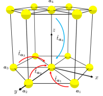
Figure 1: The simplified lattice structure of a Cu-doped Bi₂Se₃. The arrow indicates the hopping.

In the hexagonal lattice, the primitive lattice vectors are $\left(\sqrt{3}a/2,a/2,0\right)$, $\left(0,a,0\right)$, $\left(0,0,c\right)$ where $a$ and $c$ are the lattice constants in the $xy$ plane and along the $z$ axis, respectively. We define the nearest neighbor vectors $\bm{a}_{1}=\left(\sqrt{3}a/2,a/2,0\right)$, $\bm{a}_{2}=\left(0,a,0\right)$, $\bm{a}_{3}=\left(-\sqrt{3}a/2,a/2,0\right)$, and $\bm{a}_{4}=\left(0,0,c\right)$. The tight-binding Hamiltonian in real space can be written as Hashimoto et al. (2013); Mao et al. (2011)

$$H_{N} =\sum_{\bm{R}}\bm{\psi}^{{\dagger}}_{\bm{R}}\check{\varepsilon}\bm{\psi}_{\bm{R}}+\sum_{\bm{R},i}\bm{\psi}^{{\dagger}}_{\bm{R}}\check{t}_{\bm{a}_{i}}\bm{\psi}_{\bm{R}+\bm{a}_{i}}+\mathrm{H.c.},$$ (1)

$$\bm{\psi}_{\bm{R}} =\left[\psi_{P1_{z}^{+},\uparrow}(\bm{R})\,,\,\psi_{P2_{z}^{-},\uparrow}(\bm{R})\,,\,\psi_{P1_{z}^{+},\downarrow}(\bm{R})\,,\,\psi_{P2_{z}^{-},\downarrow}(\bm{R})\right]^{\mathrm{T}},$$ (2)

where $\psi^{{\dagger}}_{\sigma,s}\ \left(\psi_{\sigma,s}\right)$ is the creation (annihilation) operator of an electron at the orbital $\sigma$ ($=P1_{z}^{+}$ or $P2_{z}^{-}$) with spin $s$ ($=\uparrow$ or $\downarrow$). We consider only the nearest neighbor hopping on the hexagonal lattice in the $xy$ plane and that along the $z$ axis. An orbital $P1_{z}^{+}$ ($P2_{z}^{-}$) mainly consists of $p_{z}$ orbital of a Bi (Se) atom. The matrix element of hopping $\check{t}_{\bm{a}_{i}}$ ($i=1-4$) is described as

$$\bra{\bm{R},\sigma,s}H\ket{\bm{R}+\bm{a}_{i},\sigma^{\prime},s^{\prime}}.$$ (3)

The nearest neighbor hopping elements are illustrated in Fig. 1. In momentum space, the tight-binding Hamiltonian is described as

$$\check{H}_{N}(\bm{k}) =\check{\varepsilon}+\sum_{i}\check{t}_{\bm{a}_{i}}e^{i\bm{k}\cdot\bm{a}_{i}}+\mathrm{H.c.}.$$ (4)

The matrix structures of $\check{t}_{\bm{a}_{i}}$ are given in Appendix A. The tight-binding Hamiltonian can be written as

$$\check{H}_{N}(\bm{k}) =c_{\bm{k}}\hat{s}_{0}\hat{\sigma}_{0}+m_{\bm{k}}\hat{s}_{0}\hat{\sigma}_{3}$$

$$\hskip 42.0pt+V_{z}\hat{s}_{0}\hat{\sigma}_{2}+(V_{y}\hat{s}_{1}-V_{x}\hat{s}_{2})\hat{\sigma}_{1},$$ (5)

$$c_{\bm{k}} =-\mu+c_{1}\alpha_{1}(\bm{k})+c_{2}\alpha_{2}(\bm{k}),$$ (6)

$$m_{\bm{k}} =m_{0}+m_{1}\alpha_{1}(\bm{k})+m_{2}\alpha_{2}(\bm{k}),$$ (7)

$$V_{x,y} =v\alpha_{x,y}(\bm{k}),$$ (8)

$$V_{z} =v_{z}\alpha_{z}(\bm{k}),$$ (9)

where $\alpha_{i}(\bm{k})$ ($i=1,2,x,y,z$) is

$$\alpha_{1}(\bm{k}) =\frac{2}{c^{2}}\left(1-\cos k_{z}c\right),$$ (10)

$$\alpha_{2}(\bm{k}) =\frac{4}{3a^{2}}\left(3-2\cos\frac{\sqrt{3}k_{x}a}{2}\cos\frac{k_{y}a}{2}-\cos k_{y}a\right),$$ (11)

$$\alpha_{x}(\bm{k}) =\frac{2}{\sqrt{3}a}\sin\frac{\sqrt{3}k_{x}a}{2}\cos\frac{k_{y}a}{2},$$ (12)

$$\alpha_{y}(\bm{k}) =\frac{2}{3a}\left(\cos\frac{\sqrt{3}k_{x}a}{2}\sin\frac{k_{y}a}{2}+\sin k_{y}a\right),$$ (13)

$$\alpha_{z}(\bm{k}) =\frac{1}{c}\sin k_{z}c.$$ (14)

We define the Pauli matrices $\hat{s}_{j}$ in spin space, $\hat{\sigma}_{j}$ in orbital space, and $\hat{\tau}_{j}$ in particle-hole space for $j=1-3$. The unit matrix in these spaces are $\hat{s}_{0}$, $\hat{\sigma}_{0}$, and $\hat{\tau}_{0}$. In Eq. (5), the hopping in the $z$ direction ($\check{t}_{\bm{a}_{4}}$) causes the orbital hybridization term $V_{z}$ and the hopping in the $xy$ plane ($\check{t}_{\bm{a}_{1}},\,\check{t}_{\bm{a}_{2}},\,\check{t}_{\bm{a}_{3}}$) causes the spin-orbit interaction term $V_{x,y}$. When we expand the trigonometric functions around the $\Gamma$ point, the tight-binding Hamiltonian $\check{H}_{N}(\bm{k})$ corresponds to $\bm{k}\cdot\bm{p}$ Hamiltonian of Bi₂Se₃ Zhang et al. (2009); Liu et al. (2010).

The superconducting state in Cu_xBi₂Se₃ is described by a Hamiltonian

$$\mathcal{H}^{(0)}=\sum_{\bm{k}}\bm{\Psi}^{{\dagger}}(\bm{k})\bar{H}^{(0)}_{\bm{k}}\bm{\Psi}(\bm{k}),\quad\bm{\Psi}(\bm{k})=\left[\begin{array}[]{c}\bm{\psi}_{e}(\bm{k})\\ \bm{\psi}_{h}(\bm{k})\end{array}\right],$$ (17)

$$\bm{\psi}_{e}(\bm{k})=\left[\begin{array}[]{c}\psi_{P1_{z}^{+},\uparrow}(\bm{k})\\ \psi_{P2_{z}^{-},\uparrow}(\bm{k})\\ \psi_{P1_{z}^{+},\downarrow}(\bm{k})\\ \psi_{P2_{z}^{-},\downarrow}(\bm{k})\end{array}\right],\;\bm{\psi}_{h}(\bm{k})=\left[\begin{array}[]{c}\psi^{{\dagger}}_{P1_{z}^{+},\uparrow}(-\bm{k})\\ \psi^{{\dagger}}_{P2_{z}^{-},\uparrow}(-\bm{k})\\ \psi^{{\dagger}}_{P1_{z}^{+},\downarrow}(-\bm{k})\\ \psi^{{\dagger}}_{P2_{z}^{-},\downarrow}(-\bm{k})\end{array}\right],$$ (26)

$$\bar{H}^{(0)}_{\bm{k}}=\left(\begin{array}[]{cc}\check{H}_{N}(\bm{k})&\check{\Delta}_{\lambda}\\ \check{\Delta}^{{\dagger}}_{\lambda}&-\check{H}^{\ast}_{N}(-\bm{k})\end{array}\right).$$ (29)

According to the previous proposal Fu and Berg (2010), we consider four types of momentum-independent pair potential defined by

$$\Delta_{1} =\frac{g_{1}}{N}\sum_{\bm{k}}\langle\psi_{P1_{z}^{+},\uparrow}(\bm{k})\psi_{P1_{z}^{+},\downarrow}(-\bm{k})\rangle$$

$$=\frac{g_{1}}{N}\sum_{\bm{k}}\langle\psi_{P2_{z}^{-},\uparrow}(\bm{k})\psi_{P2_{z}^{-},\downarrow}(-\bm{k})\rangle,$$ (30)

$$\Delta_{2} =\frac{g_{2}}{N}\sum_{\bm{k}}\langle\psi_{P1_{z}^{+},\uparrow}(\bm{k})\psi_{P2_{z}^{-},\downarrow}(-\bm{k})\rangle$$

$$=-\frac{g_{2}}{N}\sum_{\bm{k}}\langle\psi_{P2_{z}^{-},\uparrow}(\bm{k})\psi_{P1_{z}^{+},\downarrow}(-\bm{k})\rangle,$$ (31)

$$\Delta_{3} =\frac{g_{3}}{N}\sum_{\bm{k}}\langle\psi_{P1_{z}^{+},\uparrow}(\bm{k})\psi_{P2_{z}^{-},\downarrow}(-\bm{k})\rangle$$

$$=\frac{g_{3}}{N}\sum_{\bm{k}}\langle\psi_{P2_{z}^{-},\uparrow}(\bm{k})\psi_{P1_{z}^{+},\downarrow}(-\bm{k})\rangle,$$ (32)

$$\Delta_{4} =\frac{g_{4}}{N}\sum_{\bm{k}}\langle\psi_{P1_{z}^{+},\uparrow}(\bm{k})\psi_{P2_{z}^{-},\uparrow}(-\bm{k})\rangle$$

$$=-\frac{g_{4}}{N}\sum_{\bm{k}}\langle\psi_{P2_{z}^{-},\uparrow}(\bm{k})\psi_{P1_{z}^{+},\uparrow}(-\bm{k})\rangle,$$ (33)

where $g_{\lambda}>0\ (\lambda=1-4)$ represents the attractive interaction between two electrons. Generally speaking, the pair correlation function can be represented as

$$f_{s,\sigma;s^{\prime},\sigma^{\prime}}(\bm{k})=\left\langle\psi_{s,\sigma}(\bm{k})\,\psi_{s^{\prime},\sigma^{\prime}}(-\bm{k})\right\rangle,$$ (34)

where we assume a spatially uniform equal-time Cooper pair. The momentum-symmetry is even-parity $s$-wave symmetry, which is a common property among the four candidates in a Cu-doped Bi₂Se₃. Because of the Fermi-Dirac statistics of electrons, the pairing correlation obeys

$$f_{s,\sigma;s^{\prime},\sigma^{\prime}}(\bm{k})=-f_{s^{\prime},\sigma^{\prime};s,\sigma}(\bm{k}).$$ (35)

The remaining symmetry options of the pairing function are orbitals and spins of a Cooper pair. Therefore, the pairing function must be either antisymmetric under $s\leftrightarrow s^{\prime}$ or antisymmetric under $\sigma\leftrightarrow\sigma^{\prime}$.

Both Eqs. (II.1) and (II.1) belong to spin-singlet symmetry. Thus the pairing functions belong to even-orbital parity. In Eq. (II.1), a Cooper pair consists of two electrons in the different orbitals (interorbital pair): one electron is in $P1_{z}^{+}$ orbital and the other is in $P2_{z}^{-}$ orbital. In Eq. (II.1), on the other hand, a Cooper pair consists of two electrons in the same orbital (intraorbital pair). The pair potential in the $P1_{z}^{+}$ orbital and that in the $P2_{z}^{-}$ orbital have the same amplitude and the same sign.

Both Eqs. (II.1) and (II.1) represent the spin-triplet interorbital pairing correlations. In these cases, the pair correlation belongs to odd-orbital-parity symmetry. In addition to the symmetry options for Cooper pairing, the pair potentials are classified by the irreducible representation of $D_{3d}$ point group. $\Delta_{2}$ and $\Delta_{4}$ can be distinguished from each other by the irreducible representation. The matrix form of pair potentials, the irreducible representation, spin symmetry, and orbital-parity of the pair potentials are summarized in Table 1. Although Fu and Berg Fu and Berg (2010) proposed a pair potential of $\Delta(i\hat{s}_{2})\hat{\sigma}_{3}$, it is unitary equivalent to Eq. (II.1) as long as the Hamiltonian $\bar{H}^{(0)}_{\bm{k}}$ preserves time-reversal symmetry Asano and Golubov (2018). (See Appendix B for details.) They also considered a pair potential of $\Delta\hat{s}_{0}(i\hat{\sigma}_{2})$ independently of Eq. (II.1). However, the behavior of $T_{c}$ under the potential disorder in the two pair potentials are the same with each other. Thus, in this paper, we discuss effects of random impurity scatterings on superconducting states described by Eqs. (II.1)-(II.1). We note that the orbital parity and the momentum parity are independent symmetry options of each other. The former represents symmetry of correlation function under the commutation of two orbitals. The latter is derived from inversion symmetry of the lattice structure.

Table 1: Symmetry classification of pair potentials. Equal-time pairing order parameter belongs to even-frequency symmetry. A spin-singlet component is described by $i\hat{s}_{2}$. An opposite-spin-triplet and an equal-spin-triplet components are indicated by $\hat{s}_{1}$ and $\hat{s}_{3}$, respectively.

Matrix	Rep.	Frequency	Spin	Momentum parity	Orbital parity
$\Delta_{1}(i\hat{s}_{2})\hat{\sigma}_{0}$	$A_{1g}$	Even	Singlet	Even	Even (Intra)
$\Delta_{2}\hat{s}_{1}(i\hat{\sigma}_{2})$	$A_{1u}$	Even	Triplet	Even	Odd (Inter)
$\Delta_{3}(i\hat{s}_{2})\hat{\sigma}_{1}$	$A_{2u}$	Even	Singlet	Even	Even (Inter)
$\Delta_{4}\hat{s}_{3}(i\hat{\sigma}_{2})$	$E_{u}$	Even	Triplet	Even	Odd (Inter)

II.2 Gor’kov equation

The Matsubara Green’s function is obtained by solving the Gor’kov equation,

$$\left[i\omega_{n}-\check{H}^{(0)}(\bm{k})\right]\bar{G}^{(0)}(\bm{k},i\omega_{n})=1,$$ (36)

$$\bar{G}^{(0)}(\bm{k},i\omega_{n})=\left(\begin{array}[]{cc}\check{\mathcal{G}}^{(0)}(\bm{k},i\omega_{n})&\check{\mathcal{F}}^{(0)}_{\lambda}(\bm{k},i\omega_{n})\\ -{\check{\mathcal{F}}^{(0)\ast}_{\lambda}}(-\bm{k},i\omega_{n})&-{\check{\mathcal{G}}^{(0)\ast}}(-\bm{k},i\omega_{n})\end{array}\right),$$ (39)

where $\omega_{n}=(2n+1)\pi T$ is a fermionic Matsubara frequency and $T$ is a temperature. To discuss the transition temperature, we need to find the solutions of Eq. (36) within the first order of $\Delta$. The results of the normal part

$$\check{\mathcal{G}}^{(0)}(\bm{k},i\omega_{n}) =\frac{1}{X}\left[\left(i\omega_{n}-c_{\bm{k}}\right)\,\hat{s}_{0}\hat{\sigma}_{0}+m_{\bm{k}}\,\hat{s}_{0}\hat{\sigma}_{3}+V_{z}\,\hat{s}_{0}\hat{\sigma}_{2}+(V_{y}\hat{s}_{1}-V_{x}\hat{s}_{2})\,\hat{\sigma}_{1}\right],$$ (40)

$$X(\bm{k},i\omega_{n}) =(i\omega_{n}-c_{\bm{k}})^{2}-m_{\bm{k}}^{2}-V_{x}^{2}-V_{y}^{2}-V_{z}^{2},$$ (41)

are common for all the pair potentials because the normal Green’s function does not include the pair potential at the lowest order. The results of anomalous Green’s function are given by,

$$\check{\mathcal{F}}^{(0)}_{1}(\bm{k},i\omega_{n}) =\frac{\Delta_{1}}{Z}\left[-i\left(\omega^{2}_{n}+c^{2}_{\bm{k}}+m^{2}_{\bm{k}}+V^{2}_{x}+V_{y}^{2}+V_{z}^{2}\right)\,\hat{s}_{2}\hat{\sigma}_{0}\right.$$

$$\hskip 24.0pt\left.+2ic_{\bm{k}}m_{\bm{k}}\,\hat{s}_{2}\hat{\sigma}_{3}+2ic_{\bm{k}}V_{z}\,\hat{s}_{2}\hat{\sigma}_{2}-2c_{\bm{k}}V_{y}\,\hat{s}_{3}\hat{\sigma}_{1}-2ic_{\bm{k}}V_{x}\,\hat{s}_{0}\hat{\sigma}_{1}\right],$$ (42)

$$\check{\mathcal{F}}^{(0)}_{2}(\bm{k},i\omega_{n}) =\frac{\Delta_{2}}{Z}\left[-i\left(\omega^{2}_{n}+c^{2}_{\bm{k}}-m^{2}_{\bm{k}}+V_{x}^{2}+V_{y}^{2}+V_{z}^{2}\right)\,\hat{s}_{1}\hat{\sigma}_{2}\right.$$

$$\hskip 24.0pt+2m_{\bm{k}}V_{y}\,\hat{s}_{0}\hat{\sigma}_{0}-2c_{\bm{k}}V_{y}\,\hat{s}_{0}\hat{\sigma}_{3}+2im_{\bm{k}}V_{x}\,\hat{s}_{3}\hat{\sigma}_{0}-2ic_{\bm{k}}V_{x}\,\hat{s}_{3}\hat{\sigma}_{3}$$

$$\hskip 24.0pt\left.+2ic_{\bm{k}}V_{z}\,\hat{s}_{1}\hat{\sigma}_{0}-2im_{\bm{k}}V_{z}\,\hat{s}_{1}\hat{\sigma}_{3}+2i\omega_{n}m_{\bm{k}}\,\hat{s}_{1}\hat{\sigma}_{1}\right],$$ (43)

$$\check{\mathcal{F}}^{(0)}_{3}(\bm{k},i\omega_{n}) =\frac{\Delta_{3}}{Z}\left[-i\left(\omega^{2}_{n}+c^{2}_{\bm{k}}-m^{2}_{\bm{k}}+V_{x}^{2}+V_{y}^{2}-V_{z}^{2})\right)\,\hat{s}_{2}\hat{\sigma}_{1}\right.$$

$$\hskip 24.0pt+2iV_{x}V_{z}\,\hat{s}_{0}\hat{\sigma}_{2}+2V_{y}V_{z}\,\hat{s}_{3}\hat{\sigma}_{2}-2ic_{\bm{k}}V_{x}\,\hat{s}_{0}\hat{\sigma}_{0}+2im_{\bm{k}}V_{x}\,\hat{s}_{0}\hat{\sigma}_{3}$$

$$\hskip 24.0pt\left.-2c_{\bm{k}}V_{y}\,\hat{s}_{3}\hat{\sigma}_{0}+2m_{\bm{k}}V_{y}\,\hat{s}_{3}\hat{\sigma}_{3}-2i\omega_{n}m_{\bm{k}}\,\hat{s}_{2}\hat{\sigma}_{2}+2i\omega_{n}V_{z}\,\hat{s}_{2}\hat{\sigma}_{3}\right],$$ (44)

$$\check{\mathcal{F}}^{(0)}_{4}(\bm{k},i\omega_{n}) =\frac{\Delta_{4}}{Z}\left[-i\left(\omega^{2}_{n}+c^{2}_{\bm{k}}-m^{2}_{\bm{k}}+V_{x}^{2}-V_{y}^{2}+V_{z}^{2}\right)\,\hat{s}_{3}\hat{\sigma}_{2}\right.$$

$$\hskip 24.0pt-2V_{x}V_{y}\,\hat{s}_{0}\hat{\sigma}_{2}-2im_{\bm{k}}\,V_{x}\hat{s}_{1}\hat{\sigma}_{0}+2ic_{\bm{k}}V_{x}\,\hat{s}_{1}\hat{\sigma}_{3}+2ic_{\bm{k}}V_{z}\,\hat{s}_{3}\hat{\sigma}_{0}$$

$$\hskip 24.0pt\left.-2im_{\bm{k}}V_{z}\,\hat{s}_{3}\hat{\sigma}_{3}-2V_{y}V_{z}\,\hat{s}_{2}\hat{\sigma}_{1}+2i\omega_{n}m_{\bm{k}}\,\hat{s}_{3}\hat{\sigma}_{1}-2\omega_{n}V_{y}\,\hat{s}_{2}\hat{\sigma}_{3}\right],$$ (45)

with $Z(\bm{k},i\omega_{n})=|X(\bm{k},i\omega_{n})|^{2}$. The $\hat{s}_{2}\hat{\sigma}_{0}$ component in Eq. (42), the $\hat{s}_{1}\hat{\sigma}_{2}$ component in Eq. (43), the $\hat{s}_{2}\hat{\sigma}_{1}$ component in Eq. (44), and the $\hat{s}_{3}\hat{\sigma}_{2}$ component in Eq. (45) are linked to the pair potentials $\Delta_{1}$, $\Delta_{2}$, $\Delta_{3}$, and $\Delta_{4}$, respectively. Therefore, the gap equations in the linear regime result in

$$\Delta_{1} =-g_{1}T\sum_{\omega_{n}}\frac{1}{N}\sum_{\bm{k}}\mathrm{Tr}\left[\check{\mathcal{F}}^{(0)}_{1}(\bm{k},i\omega_{n})\frac{(-i\hat{s}_{2})\hat{\sigma}_{0}}{4}\right]$$

$$=g_{1}T\sum_{\omega_{n}}\frac{1}{N}\sum_{\bm{k}}\frac{\Delta_{1}}{Z(\bm{k},i\omega_{n})}\left[\omega_{n}^{2}+c_{\bm{k}}^{2}+m_{\bm{k}}^{2}+V_{x}^{2}+V_{y}^{2}+V_{z}^{2}\right],$$ (46)

$$\Delta_{2} =-g_{2}T\sum_{\omega_{n}}\frac{1}{N}\sum_{\bm{k}}\mathrm{Tr}\left[\check{\mathcal{F}}^{(0)}_{2}(\bm{k},i\omega_{n})\frac{\hat{s}_{1}(-i\hat{\sigma}_{2})}{4}\right]$$

$$=g_{2}T\sum_{\omega_{n}}\frac{1}{N}\sum_{\bm{k}}\frac{\Delta_{2}}{Z(\bm{k},i\omega_{n})}\left[\omega_{n}^{2}+c^{2}_{\bm{k}}-m_{\bm{k}}^{2}+V_{x}^{2}+V_{y}^{2}+V_{z}^{2}\right],$$ (47)

$$\Delta_{3} =-g_{3}T\sum_{\omega_{n}}\frac{1}{N}\sum_{\bm{k}}\mathrm{Tr}\left[\check{\mathcal{F}}^{(0)}_{3}(\bm{k},i\omega_{n})\frac{(-i\hat{s}_{2})\hat{\sigma}_{1}}{4}\right]$$

$$=g_{3}T\sum_{\omega_{n}}\frac{1}{N}\sum_{\bm{k}}\frac{\Delta_{3}}{Z(\bm{k},i\omega_{n})}\left[\omega_{n}^{2}+c_{\bm{k}}^{2}-m_{\bm{k}}^{2}+V_{x}^{2}+V_{y}^{2}-V_{z}^{2}\right],$$ (48)

$$\Delta_{4} =-g_{4}T\sum_{\omega_{n}}\frac{1}{N}\sum_{\bm{k}}\mathrm{Tr}\left[\check{\mathcal{F}}^{(0)}_{4}(\bm{k},i\omega_{n})\frac{\hat{s}_{3}(-i\hat{\sigma}_{2})}{4}\right]$$

$$=g_{4}T\sum_{\omega_{n}}\frac{1}{N}\sum_{\bm{k}}\frac{\Delta_{4}}{Z(\bm{k},i\omega_{n})}\left[\omega_{n}^{2}+c_{\bm{k}}^{2}-m_{\bm{k}}^{2}+V_{x}^{2}-V_{y}^{2}+V_{z}^{2}\right].$$ (49)

Eqs. (42), (43), (44), and (45) show that the orbital hybridization ($V_{z}$), the spin-orbit interaction ($V_{x,y}$), and the asymmetry between the two orbitals ($m_{\bm{k}}$) generate various paring correlations which belong to different symmetry classes from that of the pair potential Black-Schaffer and Balatsky (2013); Asano and Sasaki (2015). Especially, we discuss briefly a role of odd-frequency pairing correlation in the gap equation. For instance, the pairing correlation $\check{\mathcal{F}}^{(0)}_{2}$ includes $2i\omega_{n}m_{\bm{k}}\,\hat{s}_{1}\hat{\sigma}_{1}$ which describes a spin-triplet even-orbital-parity component. Such an component must be odd-frequency symmetry because the pairing correlation function must be antisymmetric under the permutation of two electrons. In the gap equation, the odd-frequency pairing component decreases the numerator as shown in $-m_{\bm{k}}^{2}$ in Eq. (47). It has been pointed out that an odd-frequency pair decreases the transition temperature Asano and Sasaki (2015). If we would be able to tune the parameters to delete more the odd-frequency components, the gap equation results in higher $T_{c}$.

III Effects of disorder

We consider the random nonmagnetic impurities described by

$$\bar{H}_{\mathrm{imp}}(\bm{R}) =V_{\mathrm{imp}}(\bm{R})\ \hat{\tau}_{3}\hat{s}_{0}(\hat{\sigma}_{0}+\hat{\sigma}_{1}).$$ (50)

The schematic picture of potential disorder in a Cu_xBi₂Se₃ is shown in Fig. 2.

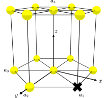
Figure 2: A model of the random potential in a Cu_xBi₂Se₃. The cross mark denotes an impurity.

We assume the impurity potential satisfies the following properties,

$$\overline{V_{\mathrm{imp}}(\bm{R})}=0,$$ (51)

$$\overline{V_{\mathrm{imp}}(\bm{R})V_{\mathrm{imp}}(\bm{R}^{\prime})}=n_{\mathrm{imp}}v^{2}_{\mathrm{imp}}\delta_{\bm{R},\bm{R}^{\prime}},$$ (52)

where $\overline{\cdots}$ means the ensemble average, $n_{\mathrm{imp}}$ is the density of the impurities, and $v_{\mathrm{imp}}$ is the strength of the impurity potential. We also assume that the attractive interactions between two electrons are insensitive to the impurity potentials Anderson (1959). We calculate the Green’s function in the presence of the impurity potentials within the Born approximation. The Green’s function is expanded up to the second order of the impurity potential.

$$\bar{G} (\bm{R}-\bm{R}^{\prime},\omega_{n})\approx\bar{G}^{(0)}(\bm{R}-\bm{R}^{\prime},\omega_{n})$$

$$+\sum_{\bm{R}_{1}}\bar{G}^{(0)}(\bm{R}-\bm{R}_{1},\omega_{n})\overline{\bar{H}_{\mathrm{imp}}(\bm{R}_{1})}\bar{G}^{(0)}(\bm{R}_{1}-\bm{R}^{\prime},\omega_{n})$$

$$+\sum_{\bm{R}_{1},\bm{R}_{2}}\bar{G}^{(0)}(\bm{R}-\bm{R}_{1},\omega_{n})$$

$$\times\overline{\bar{H}_{\mathrm{imp}}(\bm{R}_{1})\bar{G}^{(0)}(\bm{R}_{1}-\bm{R}_{2},\omega_{n})\bar{H}_{\mathrm{imp}}(\bm{R}_{2})}$$

$$\times\bar{G}(\bm{R}_{2}-\bm{R}^{\prime},\omega_{n}),$$ (53)

$$\approx \bar{G}^{(0)}(\bm{R}-\bm{R}^{\prime},\omega_{n})$$

$$+n_{\mathrm{imp}}v^{2}_{\mathrm{imp}}\sum_{\bm{R}_{1}}\bar{G}^{(0)}(\bm{R}-\bm{R}_{1},\omega_{n})\,\hat{\tau}_{3}\,\hat{s}_{0}\,\hat{\sigma}_{0}$$

$$\times\bar{G}^{(0)}(0,\omega_{n})\,\hat{\tau}_{3}\,\hat{s}_{0}\,\hat{\sigma}_{0}\bar{G}(\bm{R}_{1}-\bm{R}^{\prime},\omega_{n})$$

$$+n_{\mathrm{imp}}v^{2}_{\mathrm{imp}}\sum_{\bm{R}_{1}}\bar{G}^{(0)}(\bm{R}-\bm{R}_{1},\omega_{n})\,\hat{\tau}_{3}\,\hat{s}_{0}\,\hat{\sigma}_{1}$$

$$\times\bar{G}^{(0)}(0,\omega_{n})\,\hat{\tau}_{3}\,\hat{s}_{0}\,\hat{\sigma}_{1}\bar{G}(\bm{R}_{1}-\bm{R}^{\prime},\omega_{n}).$$ (54)

We transform the Eq. (III) to (III) by using the properties in Eqs. (51) and (52). In momentum space, Eq. (III) becomes

$$\bar{G}(\bm{k},i\omega_{n})=\bar{G}^{(0)}(\bm{k},i\omega_{n})+\bar{G}^{(0)}(\bm{k},i\omega_{n})\bar{\Sigma}_{\mathrm{imp}}\bar{G}(\bm{k},i\omega_{n}),$$ (55)

$$\bar{\Sigma}_{\mathrm{imp}}=\bar{\Sigma}_{\mathrm{intra}}+\bar{\Sigma}_{\mathrm{inter}},$$ (56)

$$\bar{\Sigma}_{\mathrm{intra}}=n_{\mathrm{imp}}v^{2}_{{\mathrm{imp}}}\hat{\tau}_{3}\hat{s}_{0}\hat{\sigma}_{0}\frac{1}{N}\sum_{\bm{k}}\bar{G}^{(0)}(\bm{k},i\omega_{n})\hat{\tau}_{3}\hat{s}_{0}\hat{\sigma}_{0},$$ (57)

$$\bar{\Sigma}_{\mathrm{inter}}=n_{\mathrm{imp}}v^{2}_{{\mathrm{imp}}}\hat{\tau}_{3}\hat{s}_{0}\hat{\sigma}_{1}\frac{1}{N}\sum_{\bm{k}}\bar{G}^{(0)}(\bm{k},i\omega_{n})\hat{\tau}_{3}\hat{s}_{0}\hat{\sigma}_{1},$$ (58)

where $\bar{\Sigma}_{\mathrm{intra}}$ and $\bar{\Sigma}_{\mathrm{inter}}$ are the self-energy due to the intraorbital impurity scatterings and that of the interorbital impurity scatterings, respectively. We describe the total self-energy as follows.

$$\bar{\Sigma}_{\mathrm{imp}}=\bar{\Sigma}_{\mathrm{intra}}+\bar{\Sigma}_{\mathrm{inter}}=\left[\begin{array}[]{cc}\check{\Sigma}_{g}&\check{\Sigma}_{f_{\lambda}}\\ -\check{\Sigma}_{f_{\lambda}}^{\ast}&-\check{\Sigma}_{g}^{\ast}\end{array}\right],$$ (61)

$$\check{\Sigma}_{g}=n_{\mathrm{imp}}v^{2}_{\mathrm{imp}}[\check{g}^{(0)}+\hat{s}_{0}\hat{\sigma}_{1}\check{g}^{(0)}\hat{s}_{0}\hat{\sigma}_{1}],$$ (62)

$$\check{\Sigma}_{f_{\lambda}}=-n_{\mathrm{imp}}v^{2}_{\mathrm{imp}}[\check{f}_{\lambda}^{(0)}+\hat{s}_{0}\hat{\sigma}_{1}\check{f}_{\lambda}^{(0)}\hat{s}_{0}\hat{\sigma}_{1}],$$ (63)

where we denote the momentum summation of the Green’s function as $1/N\sum_{\bm{k}}\check{\mathcal{G}}^{(0)}(\bm{k},i\omega_{n})=\check{g}^{(0)}$ and $1/N\sum_{\bm{k}}\check{\mathcal{F}}^{(0)}(\bm{k},i\omega_{n})=\check{f}^{(0)}$. Therefore, the Gor’kov equation in the presence of the impurity potential is described by

$$\left[i\omega_{n}-\bar{H}_{0}(\bm{k})-\bar{\Sigma}_{\mathrm{imp}}\right]\bar{G}(\bm{k},i\omega_{n})=1,$$ (64)

$$\bar{G}(\bm{k},i\omega_{n})=\left(\begin{array}[]{cc}\check{\mathcal{G}}(\bm{k},i\omega_{n})&\check{\mathcal{F}}_{\lambda}(\bm{k},i\omega_{n})\\ -\check{\mathcal{F}}_{\lambda}^{\ast}(-\bm{k},i\omega_{n})&-\check{\mathcal{G}}^{\ast}(-\bm{k},i\omega_{n})\end{array}\right).$$ (67)

The normal part of self-energy ($\check{\Sigma}_{g}$) is calculated as follows.

$$\check{\Sigma}_{g}= \left[-i\omega_{n}\eta_{n}+I_{n}\right]\,\hat{s}_{0}\hat{\sigma}_{0},$$ (68)

$$\eta_{n}= n_{\mathrm{imp}}v^{2}_{\mathrm{imp}}\frac{1}{N}\sum_{\bm{k}}\frac{2}{Z}\hskip 120.0pt$$

$$\times\left[\omega_{n}^{2}+c_{\bm{k}}^{2}+m_{\bm{k}}^{2}+V_{x}^{2}+V_{y}^{2}+V_{z}^{2}\right],$$ (69)

$$I_{n}= n_{\mathrm{imp}}v^{2}_{\mathrm{imp}}\frac{1}{N}\sum_{\bm{k}}\frac{-2c_{\bm{k}}}{Z}\hskip 120.0pt$$

$$\times\left[\omega_{n}^{2}+c_{\bm{k}}^{2}-m_{\bm{k}}^{2}-V_{x}^{2}-V_{y}^{2}-V_{z}^{2}\right].$$ (70)

Within the first order of $\Delta$, the normal Green’s function becomes

$$\check{\mathcal{G}}(\bm{k},i\omega_{n}) =\check{\mathcal{G}}^{(0)}(\bm{k},i\tilde{\omega}_{n})|_{\mu\rightarrow\tilde{\mu}},$$ (71)

$$\tilde{\omega}_{n} =\omega_{n}(1+\eta_{n}),$$ (72)

$$\tilde{\mu} =\mu-I_{n}.$$ (73)

The imaginary (real) part of the self-energy renormalizes the Matsubara frequency (chemical potential). The anomalous Green’s function after summing up the momenta is described as

$$\check{f}^{(0)}_{1} =\frac{1}{N}\sum_{\bm{k}}\frac{\Delta_{1}}{Z}\hskip 168.0pt$$

$$\times\left[-i\left(\omega_{n}^{2}+c_{\bm{k}}^{2}+m_{\bm{k}}^{2}+V_{x}^{2}+V_{y}^{2}+V_{z}^{2}\right)\,\hat{s}_{2}\hat{\sigma}_{0}\right.$$

$$\hskip 12.0pt\left.+2icm\,\hat{s}_{2}\hat{\sigma}_{3}\right],$$ (74)

$$\check{f}^{(0)}_{2} =\frac{1}{N}\sum_{\bm{k}}\frac{\Delta_{2}}{Z}\hskip 168.0pt$$

$$\times\left[-i\left(\omega_{n}^{2}+c_{\bm{k}}^{2}-m_{\bm{k}}^{2}+V_{x}^{2}+V_{y}^{2}+V_{z}^{2}\right)\,\hat{s}_{1}\hat{\sigma}_{2}\right.$$

$$\hskip 12.0pt\left.+2i\omega_{n}m_{\bm{k}}\,\hat{s}_{1}\hat{\sigma}_{1}\right],$$ (75)

$$\check{f}^{(0)}_{3} =\frac{1}{N}\sum_{\bm{k}}\frac{\Delta_{3}}{Z}\hskip 168.0pt$$

$$\times\left[-i\left(\omega_{n}^{2}+c_{\bm{k}}^{2}-m_{\bm{k}}^{2}+V_{x}^{2}+V_{y}^{2}-V_{z}^{2}\right)\,\hat{s}_{2}\hat{\sigma}_{1}\right.$$

$$\hskip 12.0pt\left.-2i\omega_{n}m\,\hat{s}_{2}\hat{\sigma}_{2}\right],$$ (76)

$$\check{f}^{(0)}_{4} =\frac{1}{N}\sum_{\bm{k}}\frac{\Delta_{4}}{Z}\hskip 168.0pt$$

$$\times\left[-i\left(\omega_{n}^{2}+c_{\bm{k}}^{2}-m_{\bm{k}}^{2}+V_{x}^{2}-V_{y}^{2}+V_{z}^{2}\right)\,\hat{s}_{3}\hat{\sigma}_{2}\right.$$

$$\hskip 12.0pt\left.+2i\omega_{n}m_{\bm{k}}\,\hat{s}_{3}\hat{\sigma}_{1}\right].$$ (77)

By substituting these expressions into Eq. (63), we obtain the anomalous part of the self-energy for each pair potential.

$$\check{\Sigma}_{f_{1}} =\Delta_{1}(i\hat{s}_{2})\hat{\sigma}_{0}\cdot\eta_{n},$$ (78)

$$\check{\Sigma}_{f_{2}} =\Delta_{2}\hat{s}_{1}\hat{\sigma}_{1}\cdot(-i\omega_{n})J_{n},$$ (79)

$$\check{\Sigma}_{f_{3}} =\Delta_{3}(i\hat{s}_{2})\hat{\sigma}_{1}\cdot\eta^{\prime}_{n},$$ (80)

$$\check{\Sigma}_{f_{4}} =\Delta_{4}\hat{s}_{3}\hat{\sigma}_{1}\cdot(-i\omega_{n})J_{n},$$ (81)

$$\eta^{\prime}_{n} =n_{\mathrm{imp}}v^{2}_{\mathrm{imp}}\frac{1}{N}\sum_{\bm{k}}\frac{2}{Z}\hskip 120.0pt$$

$$\hskip 36.0pt\times\left[\omega_{n}^{2}+c_{\bm{k}}^{2}-m_{\bm{k}}^{2}+V_{x}^{2}+V_{y}^{2}-V_{z}^{2}\right],$$ (82)

$$J_{n} =n_{\mathrm{imp}}v^{2}_{\mathrm{imp}}\frac{1}{N}\sum_{\bm{k}}\frac{4m_{\bm{k}}}{Z}.$$ (83)

Before demonstrating $T_{c}$ under the potential disorder, we briefly summarize a relation between the self-energy and the pair potential in the four cases. The results in Eq. (78) show that $\check{\Sigma}_{f_{1}}$ has the same matrix structure with the pair potential as shown in Table. 1. Namely, $\check{\Sigma}_{f_{1}}$ renormalizes the pair potential $\Delta_{1}$ which belongs to even-frequency spin-singlet even-momentum-parity even-orbital-parity (ESEE) pairing symmetry. We will show that this fact explains the robustness of $\Delta_{1}$ in the presence of impurity scatterings. The same feature can be seen in $\check{\Sigma}_{f_{3}}$ in Eq. (80), which implies the robustness of $\Delta_{3}$. On the other hand, $\check{\Sigma}_{f_{2}}$ and $\check{\Sigma}_{f_{4}}$ have the different matrix structure from their pair potentials shown in Table. 1. In other words, the impurity self-energy leaves the pair potentials as they are. The previous studies suggested that the superconductivity in such cases can be fragile. We also note that $\check{\Sigma}_{f_{2}}$ and $\check{\Sigma}_{f_{4}}$ enhance the pair correlation belonging to odd-frequency spin-triplet even-momentum-parity even-orbital-parity (OTEE) symmetry. In what follows, we discuss characteristic behavior of $T_{c}$ as a function of impurity concentration case by case.

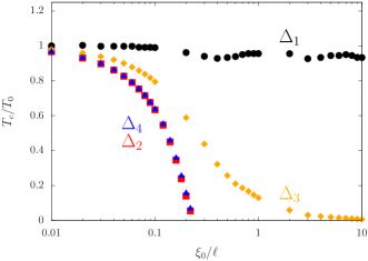
Figure 3: The superconducting transition temperature $T_{c}$ is plotted as a function of $\xi_{0}/\ell$. The vertical axis is normalized to the transition temperature in the clean limit $T_{0}$. We fix $T_{0}$ for all pair potentials.

III.0.1 $\Delta_{1}$

The gap equation for $\Delta_{1}$ results in

$$\Delta_{1} =g_{1}T\sum_{\omega_{n}}\frac{1}{N}\sum_{\bm{k}}\frac{\tilde{\Delta}_{1}}{\tilde{Z}}\hskip 84.0pt$$

$$\hskip 36.0pt\times\left[\tilde{\omega}_{n}^{2}+\tilde{c}_{\bm{k}}^{2}+m_{\bm{k}}^{2}+V_{x}^{2}+V_{y}^{2}+V_{z}^{2}\right].$$ (84)

By comparing with the gap equation in the clean limit in Eq. (46), the renormalized values are defined as

$$\tilde{\Delta}_{1} =\Delta_{1}(1+\eta_{n}),$$ (85)

$$\tilde{Z}(\bm{k},i\omega_{n}) =Z(\bm{k},i\tilde{\omega}_{n})|_{\mu\rightarrow\tilde{\mu}},$$ (86)

$$\tilde{c}_{\bm{k}} =c_{\bm{k}}|_{\mu\rightarrow\tilde{\mu}}.$$ (87)

The impurity self-energy renormalizes the pair potential and the Matsubara frequency in the same manner as $\Delta_{1}\rightarrow\tilde{\Delta}_{1}$ and $\omega_{n}\rightarrow\tilde{\omega}_{n}$ Abrikosov et al. (1975). We solve the gap equation numerically and plot the transition temperature $T_{c}$ of $\Delta_{1}$ as a function of $\xi_{0}/\ell$ in Fig. 3. Here $T_{0}$ is the transition temperature in the clean limit, $\xi_{0}=v_{F}/(2\pi T_{0})$ is the superconducting coherence length, $v_{F}$ is the Fermi velocity, $\ell=v_{F}\tau_{\mathrm{imp}}$ is the mean free path due to impurity scatterings, and $\tau_{\mathrm{imp}}$ is the lifetime of a quasiparticle. We found that the normal part of self-energy $\check{\Sigma}_{g}$ is nearly independent of the Matsubara frequency in the low energy region for $\omega_{n}\leq\omega_{c}$. Here $\omega_{c}=10^{3}T_{0}$ is the cut-off energy of the Matsubara frequency. Therefore, we estimate $\tau_{\mathrm{imp}}$ from the imaginary part of $\check{\Sigma}_{g}$ as

$$\frac{1}{\tau_{\mathrm{imp}}}=-2\mathrm{Tr}\left[\frac{1}{4}\operatorname{Im}\check{\Sigma}_{g}\right]\sim 2\pi\times n_{\mathrm{imp}}v_{\mathrm{imp}}^{2}\times 10^{-2}\,[\mathrm{eV}].$$ (88)

The horizontal axis $\xi_{0}/\ell$ in Fig. 3 is proportional to the impurity concentration $n_{\mathrm{imp}}$. The results in Fig. 3 show that $T_{c}$ of $\Delta_{1}$ is almost independent of the impurity concentration as shown with filled circles. Such behavior agrees well with $T_{c}$ in a limiting case of idealistic models. The previous papers Golubov and Mazin (1997); Efremov et al. (2011); Asano and Golubov (2018) considered two-band superconductivity with the intraband pairing order parameters (say $D_{1}$ and $D_{2}$) on idealistic two-band electronic structures and demonstrated that $T_{c}$ is independent of impurity concentration at $D_{1}=D_{2}$. The interband impurity scatterings disappear in such a symmetric situation, which explains the unchanged $T_{c}$. The superconducting state in Cu-doped Bi₂Se₃ with $\Delta_{1}$ corresponds to the symmetric intraband pairing state in the previous studies. In this paper, we confirmed that the conclusions of the previous papers on idealistic band structures are valid even if we calculate $T_{c}$ on a realistic electronic structure. In Fig. 3, the results for $\Delta_{1}$ show the oscillating behavior. Although it is not easy to specify the reasons of the oscillations, such behavior comes from a realistic band structure. In the Born approximation, we conclude that $T_{c}$ of $\Delta_{1}$ is insensitive to the impurity scatterings.

III.0.2 $\Delta_{3}$

The gap equation for $\Delta_{3}$ becomes

$$\Delta_{3} =g_{3}T\sum_{\omega_{n}}\frac{1}{N}\sum_{\bm{k}}\frac{\Delta_{3}^{\prime}}{\tilde{Z}}\hskip 84.0pt$$

$$\hskip 36.0pt\times\left[\tilde{\omega}_{n}^{2}+\tilde{c}_{\bm{k}}^{2}-m_{\bm{k}}^{2}+V_{x}^{2}+V_{y}^{2}-V_{z}^{2}\right],$$ (89)

$$\Delta_{3}^{\prime} =\Delta_{3}(1+\eta^{\prime}_{n}).$$ (90)

The pair potential is renormalized by the impurity self-energy as $\Delta_{3}\rightarrow\Delta_{3}^{\prime}$ in Eq. (89) in a slightly different way from the relation $\omega_{n}\rightarrow\tilde{\omega}_{n}$. By solving Eq. (89), we plot $T_{c}$ of $\Delta_{3}$ as a function of $\xi_{0}/\ell$ in Fig. 3. The results show that $T_{c}$ of the spin-singlet interorbital pairing order is suppressed slowly with the increase of $\xi_{0}/\ell$ and goes to zero in the dirty limit. A previous paper Asano et al. (2018), however, demonstrated on an idealistic two-band structure that $T_{c}$ of a spin-singlet $s$-wave interband pairing order is independent of the impurity concentration. Thus $\Delta_{3}$ in a Cu-doped Bi₂Se₃ is more fragile than that in an idealistic two-band model. The difference between the results in the two models can be explained by the enhancement of odd-frequency pairing components due to the realistic electronic structures. The odd-frequency pairing correlation is absent in an idealistic band structure Asano et al. (2018). As a result, the impurity self-energy renormalizes the pair potential and the Matsubara frequency in the same manner, which leads to unchanged $T_{c}$ versus $\xi_{0}/\ell$. In Cu-doped Bi₂Se₃, on the other hand, the asymmetry between two-orbitals ($m_{\bm{k}}$) and the orbital hybridization ($V_{z}$) generate the odd-frequency pairing correlations as described in Eq. (44). These correlations contribute negatively to the numerator of the renormalization factor of the pair potential $1+\eta^{\prime}_{n}$ as shown in $-m_{\bm{k}}^{2}$ and $-V_{z}^{2}$ in Eq. (III). As a consequence, the reduction of the pair potential by odd-frequency pairs causes the suppression of $T_{c}$ in the dirty regime. We conclude that the robustness of the spin-singlet $s$-wave interorbital pairing order depends on band structures.

III.0.3 $\Delta_{2}$ and $\Delta_{4}$

The gap equations for $\Delta_{2}$ and $\Delta_{4}$ result in

$$\Delta_{2} =g_{2}T\sum_{\omega_{n}}\frac{1}{N}\sum_{\bm{k}}\frac{\Delta_{2}}{\tilde{Z}}\hskip 84.0pt$$

$$\hskip 12.0pt\times\left[\tilde{\omega}_{n}^{2}+\tilde{c}_{\bm{k}}^{2}-m_{\bm{k}}^{2}+V_{x}^{2}+V_{y}^{2}+V_{z}^{2}\right.$$

$$\hskip 24.0pt\left.-2J_{n}\omega_{n}\tilde{\omega}_{n}m_{\bm{k}}\right],$$ (91)

$$\Delta_{4} =g_{4}T\sum_{\omega_{n}}\frac{1}{N}\sum_{\bm{k}}\frac{\Delta_{4}}{\tilde{Z}}\hskip 84.0pt$$

$$\hskip 12.0pt\times\left[\tilde{\omega}_{n}^{2}+\tilde{c}_{\bm{k}}^{2}-m_{\bm{k}}^{2}+V_{x}^{2}-V_{y}^{2}+V_{z}^{2}\right.$$

$$\hskip 24.0pt\left.-2J_{n}\omega_{n}\tilde{\omega}_{n}m_{\bm{k}}\right].$$ (92)

Both $\Delta_{2}$ and $\Delta_{4}$ represent spin-triplet interorbital pairing order antisymmetric under the permutation of two orbitals. The numerical results in Fig. 3 indicate that $T_{c}$ of $\Delta_{2}$ and that of $\Delta_{4}$ decrease rapidly with the increase of $\xi_{0}/\ell$ and vanish around $\xi_{0}/\ell\approx 0.3$. The impurity self-energy renormalizes the Matsubara frequency as $\omega_{n}\rightarrow\tilde{\omega}_{n}$. However, it leaves the pair potentials unchanged as shown in Eqs. (91) and (92). Therefore, $\Delta_{2}$ and $\Delta_{4}$ are fragile in the presence of impurities. The obtained results of $T_{c}$ for a Cu-doped Bi₂Se₃ agree even quantitatively with those calculated in an idealistic band structure Asano et al. (2018). The interorbital impurity scatterings mix the electronic states in the two orbitals and average the pair potentials over the two orbital degree of freedom. As a result, the impurity scatterings wash out the sign of the pair potential in Eq. (29), which leads to the suppression of odd-orbital symmetric superconductivity. We confirmed that this physical interpretation is valid independent of band structures.

Finally, we compare our results in the present paper with those in a recent study Cavanagh and Brydon (2020). The authors of Ref. Cavanagh and Brydon, 2020 formulated the random impurity scatterings based on the two-band picture in momentum space, which is obtained by diagonalizing the normal state Hamiltonian in the absence of impurities Michaeli and Fu (2012). They mapped a Hamiltonian for an interorbital $s$-wave superconductor with random impurities to a Hamiltonian for a single-band unconventional superconductor with random impurities. As a result, they concluded that $\Delta_{2}$, $\Delta_{3}$, and $\Delta_{4}$ are fragile under the potential disorder. Their conclusion for $\Delta_{3}$ does not agree with ours obtained by applying the standard method Abrikosov et al. (1975). The difference in the theoretical methods causes the discrepancy. A key point might be the self-energy due to interorbital impurity scatterings. Actually all of the previous papers Golubov and Mazin (1997); Efremov et al. (2011); Asano and Golubov (2018); Asano et al. (2018) have suggested an importance of the interorbital/interband impurity scatterings on $T_{c}$. Ref. Cavanagh and Brydon, 2020, on the other hand, does not consider the interorbital impurity scatterings.

IV Conclusion

We studied the effects of random nonmagnetic impurities on the superconducting transition temperature $T_{c}$ in Cu-doped Bi₂Se₃. We consider four types of momentum-independent pair potentials, which include the intraorbital pairing ($\Delta_{1}$), the interorbital-even-parity pairing ($\Delta_{3}$), and the interorbital-odd-parity pairings ($\Delta_{2}$ and $\Delta_{4}$). The effects of the impurity scatterings are considered through the self-energy of the Green’s function within the Born approximation. $T_{c}$ of $\Delta_{1}$ is insensitive to the impurity concentration, which is consistent with the previous theories. We find that $\Delta_{1}$ with the electronic structure of a Cu-doped Bi₂Se₃ corresponds to a limiting case of idealistic models Golubov and Mazin (1997); Efremov et al. (2011); Asano and Golubov (2018). $T_{c}$ of $\Delta_{3}$ decreases moderately with the increase of impurity concentration and vanishes in the dirty limit, which does not agree well with the results on an idealistic model Asano et al. (2018). The presence of the odd-frequency pairing correlations explain the discrepancy. $T_{c}$ of $\Delta_{2}$ and $\Delta_{4}$ decrease rapidly with the increase of the impurity concentration. Superconductivity vanishes at a critical value of the impurity concentration. The results are consistent with those in an idealistic model even quantitatively Asano et al. (2018).

We found that the robustness of the even-orbital-parity order parameters depends on the details of the band structures and that the odd-orbital-parity order parameters are fragile irrespective of the band structures.

Appendix A Restriction of hopping matrix in tight-binding Hamiltonian

The crystal structure of Bi₂Se₃ preserves discrete symmetries Zhang et al. (2009); Liu et al. (2010) such as threefold rotation $R_{3}$ along the $z$ direction, twofold rotation $R_{2}$ along the $x$ direction, and inversion $P$. In addition, both the normal and superconducting states preserve time-reversal $T$ symmetry. With the basis of ($\ket{P1_{z}^{+},\uparrow}$, $\ket{P2_{z}^{-},\uparrow}$, $\ket{P1_{z}^{+},\downarrow}$, $\ket{P2_{z}^{-},\downarrow}$), these symmetry operations can be represented as $R_{3}=\exp(i\frac{\pi}{3}s_{3}\sigma_{0})$, $R_{2}=is_{1}\sigma_{3}$, $P=s_{0}\sigma_{3}$, and $T=is_{2}\sigma_{0}\mathcal{K}$, respectively. Here $\mathcal{K}$ represents the complex conjugation.

Under threefold rotation symmetry, the relation

$$\bra{\bm{R},\sigma,s}H\ket{\bm{R}+\bm{a}_{i},\sigma^{\prime},s^{\prime}}=\exp\left(i\frac{\pi}{3}(s^{\prime}_{3}-s_{3})\right)\bra{\bm{R},\sigma,s}H\ket{\bm{R}+\bm{a}_{j},\sigma^{\prime},s^{\prime}},$$ (93)

is satisfied for $(\bm{a}_{i},\bm{a}_{j})=(\bm{a}_{1},-\bm{a}_{2})$, $(\bm{a}_{2},-\bm{a}_{3})$, and $(\bm{a}_{3},\bm{a}_{1})$. Under twofold rotation symmetry, the relation

$$\bra{\bm{R},\sigma,s}H\ket{\bm{R}+\bm{a}_{i},\sigma^{\prime},s^{\prime}}=\sigma^{\prime}_{3}\sigma_{3}\bra{\bm{R},\sigma,\overline{s}}H\ket{\bm{R}+\bm{a}_{j},\sigma^{\prime},\overline{s^{\prime}}},$$ (94)

holds true for $(\bm{a}_{i},\bm{a}_{j})$ = $(\bm{a}_{1},-\bm{a}_{3})$, $(\bm{a}_{2},-\bm{a}_{2})$, and $(\bm{a}_{3},-\bm{a}_{1})$. As a results of inversion symmetry, we find the relation of

$$\bra{\bm{R},\sigma,s}H\ket{\bm{R}+\bm{a}_{i},\sigma^{\prime},s^{\prime}}=\sigma^{\prime}_{3}\sigma_{3}\bra{\bm{R},\sigma,s}H\ket{\bm{R}-\bm{a}_{i},\sigma^{\prime},s^{\prime}}.$$ (95)

Finally, time-reversal symmetry is described as

$$\bra{\bm{R},\sigma,s}H\ket{\bm{R}+\bm{a}_{i},\sigma^{\prime},s^{\prime}}=s^{\prime}_{3}s_{3}\bra{\bm{R},\sigma^{\prime},\overline{s^{\prime}}}H\ket{\bm{R}-\bm{a}_{i},\sigma,\overline{s}}.$$ (96)

We have used the notation of

$$\sigma_{3} =\begin{cases}+1&(\sigma=P1_{z}^{+})\\ -1&(\sigma=P2_{z}^{-})\end{cases},\quad s_{3}=\begin{cases}+1&(s=\uparrow)\\ -1&(s=\downarrow)\end{cases},$$ (97)

$$\overline{\sigma} =\begin{cases}P2_{z}^{-}&(\sigma=P1_{z}^{+})\\ P1_{z}^{+}&(\sigma=P2_{z}^{-})\end{cases},\quad\overline{s}=\begin{cases}\downarrow&(s=\uparrow)\\ \uparrow&(s=\downarrow)\end{cases}.$$ (98)

According to the conditions in Eqs. (93), (94), (95), and (96), the hopping matrices can be reduced as Hashimoto et al. (2013); Mao et al. (2011)

$$\check{t}_{\bm{a}_{1}} =\left(\begin{array}[]{cccc}t_{11}&t_{12}&0&t_{14}\\ -t_{12}&t_{22}&t_{14}&0\\ 0&-t_{14}^{\ast}&t_{11}&t_{12}\\ -t_{14}^{\ast}&0&-t_{12}&t_{22}\end{array}\right),\quad\check{t}_{-\bm{a}_{1}}=\left(\begin{array}[]{cccc}t_{11}&-t_{12}&0&-t_{14}\\ t_{12}&t_{22}&-t_{14}&0\\ 0&t_{14}^{\ast}&t_{11}&-t_{12}\\ t_{14}^{\ast}&0&t_{12}&t_{22}\end{array}\right),$$ (107)

$$\check{t}_{\bm{a}_{2}} =\left(\begin{array}[]{cccc}t_{11}&-t_{12}&0&-e^{i2\pi/3}t_{14}\\ t_{12}&t_{22}&-e^{i2\pi/3}t_{14}&0\\ 0&-e^{i2\pi/3}t_{14}&t_{11}&-t_{12}\\ -e^{i2\pi/3}t_{14}&0&t_{12}&t_{22}\end{array}\right),\quad\check{t}_{-\bm{a}_{2}}=\left(\begin{array}[]{cccc}t_{11}&t_{12}&0&e^{i2\pi/3}t_{14}\\ -t_{12}&t_{22}&e^{i2\pi/3}t_{14}&0\\ 0&e^{i2\pi/3}t_{14}&t_{11}&t_{12}\\ e^{i2\pi/3}t_{14}&0&-t_{12}&t_{22}\end{array}\right),$$ (116)

$$\check{t}_{\bm{a}_{3}} =\left(\begin{array}[]{cccc}t_{11}&t_{12}&0&-t_{14}^{\ast}\\ -t_{12}&t_{22}&-t_{14}^{\ast}&0\\ 0&t_{14}&t_{11}&t_{12}\\ t_{14}&0&-t_{12}&t_{22}\end{array}\right),\quad\check{t}_{-\bm{a}_{3}}=\left(\begin{array}[]{cccc}t_{11}&-t_{12}&0&t_{14}^{\ast}\\ t_{12}&t_{22}&t_{14}^{\ast}&0\\ 0&-t_{14}&t_{11}&-t_{12}\\ -t_{14}&0&t_{12}&t_{22}\end{array}\right),$$ (125)

$$\check{t}_{\bm{a}_{4}} =\left(\begin{array}[]{cccc}t^{\prime}_{11}&t^{\prime}_{12}&0&0\\ -t^{\prime}_{12}&t^{\prime}_{22}&0&0\\ 0&0&t^{\prime}_{11}&t^{\prime}_{12}\\ 0&0&-t^{\prime}_{12}&t^{\prime}_{22}\end{array}\right),\quad\check{t}_{-\bm{a}_{4}}=\left(\begin{array}[]{cccc}t^{\prime}_{11}&-t^{\prime}_{12}&0&0\\ t^{\prime}_{12}&t^{\prime}_{22}&0&0\\ 0&0&t^{\prime}_{11}&-t^{\prime}_{12}\\ 0&0&t^{\prime}_{12}&t^{\prime}_{22}\end{array}\right).$$ (134)

In momentum space, the tight-binding Hamiltonian becomes

$$\check{H}_{N}(\bm{k}) =\left(\begin{array}[]{cccc}c_{\bm{k}}+m_{\bm{k}}&-i(v_{3}\alpha_{3}(\bm{k})+v_{z}\alpha_{z}(\bm{k}))&0&v(\alpha_{y}(\bm{k})+i\alpha_{x}(\bm{k}))\\ i(v_{3}\alpha_{3}(\bm{k})+v_{z}\alpha_{z}(\bm{k}))&c_{\bm{k}}-m_{\bm{k}}&v(\alpha_{y}(\bm{k})+i\alpha_{x}(\bm{k}))&0\\ 0&v(\alpha_{y}(\bm{k})-i\alpha_{x}(\bm{k}))&c_{\bm{k}}+m_{\bm{k}}&-i(v_{3}\alpha_{3}(\bm{k})+v_{z}\alpha_{z}(\bm{k}))\\ v(\alpha_{y}(\bm{k})-i\alpha_{x}(\bm{k}))&0&i(v_{3}\alpha_{3}(\bm{k})+v_{z}\alpha_{z}(\bm{k}))&c_{\bm{k}}-m_{\bm{k}}\end{array}\right),$$ (139)

with

$$c_{\bm{k}} =-\mu+c_{1}\alpha_{1}(\bm{k})+c_{2}\alpha_{2}(\bm{k}),\quad m_{\bm{k}}=m_{0}+m_{1}\alpha_{1}(\bm{k})+m_{2}\alpha_{2}(\bm{k}),$$ (140)

$$c_{1} =-\frac{c^{2}}{2}(t^{\prime}_{11}+t^{\prime}_{22}),\quad c_{2}=-\frac{3a^{2}}{4}(t_{11}+t_{22}),\quad\mu=-3(t_{11}+t_{22})-(t^{\prime}_{11}+t^{\prime}_{22})-\varepsilon,$$ (141)

$$m_{1} =-\frac{c^{2}}{2}(t^{\prime}_{11}-t^{\prime}_{22}),\quad m_{2}=-\frac{3a^{2}}{4}(t_{11}-t_{22}),\quad m_{0}=3(t_{11}-t_{22})+t^{\prime}_{11}-t^{\prime}_{22},$$ (142)

$$v =-3ie^{i2\pi/3}at_{14},\quad v_{z}=-2ct^{\prime}_{12},\quad v_{3}=\frac{3a^{3}}{4}t_{12}.$$ (143)

Here $\alpha_{1}(\bm{k})$, $\alpha_{2}(\bm{k})$, $\alpha_{x}(\bm{k})$, $\alpha_{y}(\bm{k})$, and $\alpha_{z}(\bm{k})$, are defined in Eqs. (10)-(14). We also define $\alpha_{3}(\bm{k})=-\frac{8}{3a^{3}}(2\cos\frac{\sqrt{3}}{2}k_{x}a\sin\frac{1}{2}k_{y}a-\sin k_{y}a)$. In this paper, we set the parameters as follows Hashimoto et al. (2013); Mizushima et al. (2014): $a=4.14~{}\mathrm{\AA}$, $c=28.7~{}\mathrm{\AA}$, $\mu=0.5~{}\mathrm{eV}$, $c_{2}=30.4~{}\mathrm{eV\AA^{2}}$, $m_{0}=-0.28~{}\mathrm{eV}$, $m_{2}=44.5~{}\mathrm{eV\AA^{2}}$, $v=3.33~{}\mathrm{eV\AA}$, $c_{1}/c^{2}=0.024~{}\mathrm{eV}$, $m_{1}/c^{2}=0.20~{}\mathrm{eV}$, and $v_{z}/c=0.32~{}\mathrm{eV}$. We choose $v_{3}=0$ for simplicity Zhang et al. (2009); Liu et al. (2010).

Appendix B Unitary equivalence of the Hamiltonian with intraorbital pairing order

The superconducting state with $s$-wave spin-singlet intraorbital pairing order is described by a following Bogoliubov-de Gennes Hamiltonian Asano and Golubov (2018).

$$\bar{H}^{(0)}_{\bm{k}}(\theta,\varphi_{1},\varphi_{2})=\left[\begin{array}[]{cccccccc}\xi_{1}&-iV_{z}e^{i\theta}&0&Ve^{i\theta}&0&0&\Delta_{P1_{z}^{+}}&0\\ iV_{z}e^{-i\theta}&\xi_{2}&Ve^{-i\theta}&0&0&0&0&\Delta_{P2_{z}^{-}}\\ 0&V^{\ast}e^{i\theta}&\xi_{1}&-iV_{z}e^{i\theta}&-\Delta_{P1_{z}^{+}}&0&0&0\\ V^{\ast}e^{-i\theta}&0&iV_{z}e^{-i\theta}&\xi_{2}&0&-\Delta_{P2_{z}^{-}}&0&0\\ 0&0&-\Delta_{P1_{z}^{+}}^{\ast}&0&-\xi_{1}&iV_{z}e^{-i\theta}&0&V^{\ast}e^{-i\theta}\\ 0&0&0&-\Delta_{P2_{z}^{-}}^{\ast}&-iV_{z}e^{i\theta}&-\xi_{2}&V^{\ast}e^{i\theta}&0\\ \Delta_{P1_{z}^{+}}^{\ast}&0&0&0&0&Ve^{-i\theta}&-\xi_{1}&iV_{z}e^{-i\theta}\\ 0&\Delta_{P2_{z}^{-}}^{\ast}&0&0&Ve^{i\theta}&0&-iV_{z}e^{i\theta}&-\xi_{2}\end{array}\right],$$ (152)

$$\xi_{1}=c_{\bm{k}}+m_{\bm{k}},\quad\xi_{2}=c_{\bm{k}}-m_{\bm{k}},\quad V=v(\alpha_{y}(\bm{k})+i\alpha_{x}(\bm{k})),\quad V_{z}=v_{z}\alpha_{z}(\bm{k}),$$ (153)

$$\Delta_{P1_{z}^{+}}=\frac{g_{P1_{z}^{+}}}{N}\sum_{\bm{k}}\langle\psi_{P1_{z}^{+},\uparrow}(\bm{k})\psi_{P1_{z}^{+},\downarrow}(-\bm{k})\rangle=|\Delta_{P1_{z}^{+}}|e^{i\varphi_{1}},$$ (154)

$$\Delta_{P2_{z}^{-}}=\frac{g_{P2_{z}^{-}}}{N}\sum_{\bm{k}}\langle\psi_{P2_{z}^{-},\uparrow}(\bm{k})\psi_{P2_{z}^{-},\downarrow}(-\bm{k})\rangle=|\Delta_{P2_{z}^{-}}|e^{i\varphi_{2}},$$ (155)

where $g_{\sigma}>0$ represents the attractive interaction between two electrons in the orbital $\sigma$ and $\theta$ denotes the phase of the hybridization in the normal state. We obtain the normal part of $\bar{H}^{(0)}_{\bm{k}}(\theta,\varphi_{1},\varphi_{2})$ from Eq. (5) by choosing $\psi_{P1_{z}^{+},s}\,\rightarrow\,\psi_{P1_{z}^{+},s}e^{i\theta/2}$ and $\psi_{P2_{z}^{-},s}\,\rightarrow\,\psi_{P2_{z}^{-},s}e^{-i\theta/2}$. Although the phase factor $e^{i\theta}$ does not affect the physics in the normal state, such a gauge transformation affects the relative phase difference between the order parameters $\varphi_{1}-\varphi_{2}$ Asano and Golubov (2018).

Time-reversal symmetry of $\bar{H}^{(0)}_{\bm{k}}$ is represented by

$$\mathcal{T}\bar{H}^{(0)}_{\bm{k}}\mathcal{T}^{-1}=\bar{H}^{(0)}_{-\bm{k}},\quad\mathcal{T}=\hat{\tau}_{0}(i\hat{s}_{2})\hat{\sigma}_{0}\mathcal{K}.$$ (156)

If we find a transformation $\bar{U}$ which eliminates all the phase factors in Eq. (152), it is possible to show time-reversal symmetry of $\bar{H}^{(0)}_{\bm{k}}$ Asano and Golubov (2018). By applying the unitary transformation,

$$\bar{U}={\mathrm{diag}}[e^{-i\varphi_{1}/2},e^{-i\varphi_{2}/2},e^{-i\varphi_{1}/2},e^{-i\varphi_{2}/2},e^{i\varphi_{1}/2},e^{i\varphi_{2}/2},e^{i\varphi_{1}/2},e^{i\varphi_{2}/2}],$$ (157)

the Hamiltonian is transformed into

$$\bar{U}\bar{H}^{(0)}_{\bm{k}}(\theta,\varphi_{1},\varphi_{2})\bar{U}^{{\dagger}}=\bar{H}^{(0)}_{\bm{k}}(\theta-\frac{\varphi_{1}-\varphi_{2}}{2},0,0).$$ (158)

Therefore, the three phases must satisfy a relation

$$2\theta-\varphi_{1}+\varphi_{2}=2\pi n,$$ (159)

with $n$ being an integer for the Hamiltonian to preserve time-reversal symmetry. By tuning $\theta=0$ at $n=0$, the two pair potentials have the same sign with each other because of $\varphi_{1}-\varphi_{2}=0$. By tuning $\theta=\pi/2$, on the other hand, $\bar{H}^{(0)}_{\bm{k}}(\pi/2,0,\pi)$ describes a state where two pair potentials have the opposite sign to each other. It is easy to show that $\bar{H}^{(0)}_{\bm{k}}(\pi/2,0,\pi)$ and $\bar{H}^{(0)}_{\bm{k}}(0,0,0)$ are unitary equivalent to each other. We set $g_{P1_{z}^{+}}=g_{P2_{z}^{-}}=g_{1}$ and $\Delta_{P1_{z}^{+}}=\Delta_{P2_{z}^{-}}=\Delta_{1}$ in section II. Under the condition, $\Delta_{1}(i\hat{s}_{2})\hat{\sigma}_{3}$ is unitary equivalent to $\check{\Delta}_{1}=\Delta_{1}(i\hat{s}_{2})\hat{\sigma}_{0}$.