A critical overview of privacy-preserving approaches
for collaborative forecasting

Abstract

Cooperation between different data owners may lead to an improvement in forecast quality – for instance by benefiting from spatial-temporal dependencies in geographically distributed time series. Due to business competitive factors and personal data protection questions, said data owners might be unwilling to share their data, which increases the interest in collaborative privacy-preserving forecasting. This paper analyses the state-of-the-art and unveils several shortcomings of existing methods in guaranteeing data privacy when employing Vector Autoregressive (VAR) models. The methods are divided into three groups: data transformation, secure multi-party computations, and decomposition methods. The analysis shows that state-of-the-art techniques have limitations in preserving data privacy, such as (i) the necessary trade-off between privacy and forecasting accuracy, empirically evaluated through simulation and real-world experiment based on solar data; (ii) the iterative model fitting processes which reveal data after a number of iterations.

1 Introduction

The progress of the internet-of-things (IoT) and big data technologies is fostering a disruptive evolution in the development of innovative data analytics methods and algorithms. This also yields ideal conditions for data-driven services (from descriptive to prescriptive analysis), in which the accessibility to large volumes of data is a fundamental requirement. In this sense, the combination of data from different owners can provide valuable information for end-users and increase their competitiveness.

In order to combine data coming from different sources, several statistical approaches have emerged. For example, in time series collaborative forecasting, the Vector Autoregressive (VAR) model has been widely used to forecast variables that may have different data owners. In the energy sector, the VAR model is deemed appropriate to update very short-term forecasts (e.g., from 15 minutes to 6 hours ahead) with recent data, thus taking advantage of geographically distributed data collected from sensors (e.g., anemometer, pyranometer) and/or wind turbines and solar power inverters [Tastu et al., 2013, Bessa et al., 2015a]. The VAR model can also be used in short-term electricity price forecasting [Ziel & Weron, 2018]. Furthermore, the large number of potential data owners favors the estimation of the VAR model’s coefficients by applying distributed optimization algorithms. The Alternating Direction Method of Multipliers (ADMM) is a widely used convex optimization technique; see Boyd et al. [2011]. The combination of the VAR model and ADMM can be used jointly for collaborative forecasting [Cavalcante et al., 2017], which consists of collecting and combining information from diverse owners. The collaborative forecasting methods require sharing data or coefficients, depending on the structure of the data, and may or may not be focused on data privacy. This process is also called federated learning [Yang et al., 2019].

Some other examples of collaborative forecasting include: (a) forecasting and inventory control in supply chains, in which the benefits of various types of information-sharing options are investigated  [Aviv, 2003, 2007]; (b) forecasting traffic flow data (i.e. speeds) among different locations [Ravi & Al-Deek, 2009]; (c) forecasting retail prices of a specific product at every outlet by using historical retail prices of the product at a target outlet and at competing outlets [Ahmad et al., 2016]. The VAR model is the simplest collaborative model but, conceptually, a collaborative forecasting model for time series does not need to be a VAR. Furthermore, it is possible to extend the VAR model to include exogenous information (see Nicholson et al. [2017] for more details) and to model non-linear relationships with past values (e.g. Li & Genton [2009] extend the additive model structure to a multivariate setting).

Setting aside the significant potential of the VAR model for collaborative forecasting, the concerns with the privacy of personal and commercially sensitive data comprise a critical barrier and require privacy-preserving algorithmic solutions for estimating the coefficients of the model.

A confidentiality breach occurs when third parties recover the data provided in confidence without consent. The leaking of a single record from the dataset may have a different impact according to the nature of the data. For example, in medical data where each record represents a different patient, it could lead to the disclosure of all the details about said patient. On the other hand, concerning renewable energy generation time series, knowing that 30 MWh was produced in a given hour does not provide very relevant information to a competitor. Hereafter, the term confidentiality breach designates the reconstruction of the entire dataset by another party.

These concerns with data confidentiality motivated the research to handle confidential data in methods such as linear regression and classification problems [Du et al., 2004], ridge linear regression [Karr et al., 2009], logistic regression [Wu et al., 2012], survival analysis [Lu et al., 2015], aggregated statistics for time series data [Jia et al., 2014], etc. Aggregated statistics consist of aggregating a set of time series data through a specific function, such as the average (e.g., average amount of daily exercise), sum, minimum or maximum. However, certain literature approaches identified confidentiality breaches, showing that the statistical methods developed to protect data privacy should be analyzed to confirm their robustness and that additional research may be required to address overlooked limitations [Fienberg et al., 2009]. Furthermore, the application of these methodologies to the VAR model needs to be carefully analyzed, since the target variables are the time series of each data owner, and the covariates are the lags of the same time series, meaning that both target and covariates share a large proportion of values.

The simplest solution would be having the data owners agreeing on a commonly trusted entity (or a central node), capable of gathering private data, solving the associated model’s fitting problem on behalf of the data owners, and then returning the results [Pinson, 2016]. However, in many cases, the data owners are unwilling to share their data even with a trusted central node. This has also motivated the development of data markets to monetize data and promote data sharing [Agarwal et al., 2019], which can be driven by blockchain and smart contracts technology [Kurtulmus & Daniel, 2018].

Another possibility would be to apply differential privacy mechanisms, which consist in adding properly calibrated noise to an algorithm (e.g., adding noise to the coefficients estimated during each iteration of the fitting procedure) or to the data itself. Differential privacy is not an algorithm, but a rigorous definition of privacy that is useful for quantifying and bounding privacy loss (i.e., how much original data a party can recover when receiving data protected with added noise) [Dwork & Smith, 2009]. It requires computations insensitive to changes in any particular record or intermediate computations, thereby restricting data leaks through the results – this is elaborated in A. While computationally efficient and popular, these techniques invariably degrade the predictive performance of the model [Yang et al., 2019] and are not very effective, as this paper shows.

The present paper conducts a review of the state-of-the-art in statistical methods for collaborative forecasting with privacy-preserving approaches. This work is not restricted to a simple overview of the existing methods and it performs a critical evaluation of said methods, from a mathematical and numerical point of view, namely when applied to the VAR model. The major contribution to the literature is to show gaps and downsides of current methods and to present insights for further improvements towards fully privacy-preserving VAR forecasting methods.

In this work, we analyze the existing state-of-the-art privacy-preserving techniques, dividing them into the following groups:

• Data transformation methods: each data owner transforms their data before the model’s fitting process, by adding randomness to the original data in such a way that high accuracy and privacy can be achieved at the end of the fitting process. The statistical method is independent of the transformation function and it is applied to the transformed data.

• Secure multi-party computation protocols: the encryption of the data occurs while fitting the statistical model (i.e. intermediate calculations of an iterative process) and data owners are required to conjointly compute a function over their data with protocols for secure matrix operations. A protocol consists of a set of rules that determine how data owners must operate to determine said function. These rules establish the calculations assigned to each data owner, what information should be shared among them, in addition to the conditions necessary for the adequate implementation of said calculations.

• Decomposition-based methods: the optimization problem is decomposed into sub-problems allowing each data owner to fit their model’s coefficients separately.

The remaining of the paper is organized as follows: Section 2 describes the state-of-the-art for collaborative forecasting with privacy-preserving; Section 3 describes the VAR model as well as coefficients estimators, and performs a critical evaluation of the state-of-the-art methods when applied to the VAR model (solar energy time series data are used in the numerical analysis). Section 4 focuses on the discussion and comparison of the presented approaches, while the conclusions are presented in Section 5.

2 Privacy-preserving Approaches

For notation purposes, vectors and matrices are denoted by bold small and capital letters, e.g. $\mathbf{a}$ and $\mathbf{A}$, respectively. The vector $\mathbf{a}=[a_{1},\dots,a_{k}]^{\top}$ represents a column vector with $k$ dimension, where $a_{i}$ are scalars, $i=1,\dots,k$. The column-wise joining of vectors and matrices is indicated by $[\mathbf{a},\mathbf{b}]$ and $[\mathbf{A},\mathbf{B}]$, respectively.

Furthermore, $\mathbf{Z}\in\mathbb{R}^{T\times M}$ is the covariate matrix and $\mathbf{Y}\in\mathbb{R}^{T\times N}$ is the target matrix, considering $n$ data owners. The values $T$, $M$ and $N$ are the number of records, covariates and target variables, respectively. When considering collaborative forecasting models, different divisions of the data may be considered. Figure 1 shows the most common one, i.e.

1. Data split by records: the data owners, represented as $A_{i},i=1,\dots,n$, observe the same features for different groups of samples, e.g. different timestamps in the case of time series. $\mathbf{Z}$ is split into $\mathbf{Z}_{A_{i}}^{r}\in\mathbb{R}^{T_{A_{i}}\times M}$ and $\mathbf{Y}$ into $\mathbf{Y}_{A_{i}}^{r}\in\mathbb{R}^{T_{A_{i}}\times N}$, such that $\sum_{i=1}^{n}T_{A_{i}}=T$;

2. Data split by features: the data owners observe different features of the same records. $\mathbf{Z}=[\mathbf{Z}_{A_{1}},\dots,\mathbf{Z}_{A_{n}}]$, $\mathbf{Y}=[\mathbf{Y}_{A_{1}},\dots,\mathbf{Y}_{A_{n}}]$, such that $\mathbf{Z}_{A_{i}}\in\mathbb{R}^{T\times M_{A_{i}}}$, $\mathbf{Y}_{A_{i}}\in\mathbb{R}^{T\times N_{A_{i}}}$, with $\sum_{i=1}^{n}M_{A_{i}}=M$ and $\sum_{i=1}^{n}N_{A_{i}}=N$;

This section summarizes state-of-the-art approaches to deal with privacy-preserving collaborative forecasting methods. Section 2.1 describes the methods that ensure confidentiality by transforming the data. Section 2.2 presents and analyzes the secure multi-party protocols. Section 2.3 describes the decomposition-based methods.

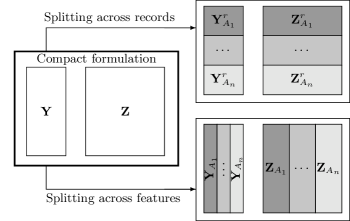
Figure 1: Common data division structures.

2.1 Data Transformation Methods

Data transformation methods use operator $\mathcal{T}$ to transform the data matrix $\mathbf{X}$ into $\tilde{\mathbf{X}}=\mathcal{T}(\mathbf{X})$. Then, the problem is solved in the transformed domain. A common method of masking sensitive data is adding or multiplying it by perturbation matrices. In additive randomization, random noise is added to the data in order to mask the values of records. Consequently, the more masked the data becomes, the more secure it will be, as long as the differential privacy definition is respected (see A). However, the use of randomized data implies the deterioration of the estimated statistical models, and the estimated coefficients of said data should be close to the estimated coefficients after using original data [Zhou et al., 2009].

Concerning multiplicative randomization, it enables changing the dimensions of the data by multiplying it by random perturbation matrices. If the perturbation matrix $\mathbf{W}\in\mathbb{R}^{k\times m}$ multiplies the original data $\mathbf{X}\in\mathbb{R}^{m\times n}$ on the left (pre-multiplication), i.e.  $\mathbf{WX}$, then it is possible to change the number of records; otherwise, if $\mathbf{W}\in\mathbb{R}^{n\times s}$ multiplies $\mathbf{X}\in\mathbb{R}^{m\times n}$ on the right (post-multiplication), i.e.  $\mathbf{XW}$, it is possible to modify the number of features. Hence, it is possible to change both dimensions by applying both pre and post-multiplication by perturbation matrices.

2.1.1 Single Data Owner

The use of linear algebra to mask the data is a common practice in recent outsourcing approaches, in which a data owner resorts to the cloud to fit their model’s coefficients, without sharing confidential data. For example, in Ma et al. [2017] the coefficients that optimize the linear regression model

$$\mathbf{y}=\mathbf{X}\boldsymbol{\beta}+\boldsymbol{\varepsilon}\ ,$$ (1)

with covariate matrix $\mathbf{X}\in\mathbb{R}^{m\times n}$, target variable $\mathbf{y}\in\mathbb{R}^{n}$, coefficient vector $\boldsymbol{\beta}\in\mathbb{R}^{n}$ and error vector $\boldsymbol{\varepsilon}\in\mathbb{R}^{n}$, are estimated through the regularized least squares estimate for the ridge linear regression, with penalization term $\lambda>0$,

$$\hat{\boldsymbol{\beta}}_{\text{ridge}}=(\mathbf{X}^{\top}\mathbf{X}+\lambda\mathbf{I})^{-1}\mathbf{X}^{\top}\mathbf{y}.$$ (2)

In order to compute $\hat{\boldsymbol{\beta}}_{\text{ridge}}$ via a cloud server, the authors consider that

$$\hat{\boldsymbol{\beta}}_{\text{ridge}}=\mathbf{A}^{-1}\mathbf{b}\ ,$$ (3)

where $\mathbf{A}=(\mathbf{X}^{\top}\mathbf{X}+\lambda\mathbf{I})^{-1}$ and $\mathbf{b}=\mathbf{X}^{\top}\mathbf{y}$, $\mathbf{A}\in\mathbb{R}^{n\times n}$, $\mathbf{b}\in\mathbb{R}^{n}$. Then, the masked matrices $\mathbf{MAN}$ and $\mathbf{M}(\mathbf{b}+\mathbf{Ar})$ are sent to the server which computes

$$\hat{\boldsymbol{\beta}}^{\prime}=(\textbf{MAN})^{-1}(\mathbf{M}(\mathbf{b}+\mathbf{Ar}))\ ,$$ (4)

where $\mathbf{M}$, $\mathbf{N}$, and $\mathbf{r}$ are randomly generated matrices, $\mathbf{M},\mathbf{N}\in\mathbb{R}^{n\times n}$, $\mathbf{r}\in\mathbb{R}^{n}$. Finally, the data owner receives $\hat{\boldsymbol{\beta}}^{\prime}$ and recovers the original coefficients by computing $\hat{\boldsymbol{\beta}}_{\text{ridge}}=\mathbf{N}\hat{\boldsymbol{\beta}}^{\prime}-\mathbf{r}$.

Data normalization is also a data transformation approach that masks data by transforming the original features into a new range through the use of a mathematical function. There are many methods for data normalization, the most important ones being $z$-score and min-max normalization [Jain & Bhandare, 2011], which are useful when the actual minimum and maximum values of the features are unknown. However, in many applications, these values are either known or publicly available, and normalized values still encompass commercially valuable information.

As to time series data, other approaches for data randomization make use of the Fourier and wavelet transforms. The Fourier transform allows representing periodic time series as a linear combination of sinusoidal components (sine and cosine). In Papadimitriou et al. [2007], each data owner generates a noise time series by: (i) adding Gaussian noise to relevant coefficients, or (ii) disrupting each sinusoidal component by randomly changing its magnitude and phase. Similarly, the wavelet transform represents the time series as a combination of functions (e.g. the Mexican hat or the Poisson wavelets), and randomness can be introduced by adding random noise to the coefficients [Papadimitriou et al., 2007]. However, there are no privacy guarantees since noise does not respect any formal definition such as differential privacy.

2.1.2 Multiple Data Owners

The task of masking data is even more challenging when dealing with different data owners, since it is crucial to ensure that the transformations that data owners make to their data preserve the real relationship between the variables or the time series.

Usually, for generalized linear models (linear regression model, logistic regression model, among others), where $n$ data owners observe the same features, i.e. data is split by records as illustrated in Figure 1, each data owner $A_{i},i=1,...,n$, can individually multiply their covariate matrix $\mathbf{Z}^{r}_{A_{i}}\in\mathbb{R}^{{T_{A_{i}}\times M}}$ and target variable $\mathbf{Y}^{r}_{A_{i}}\in\mathbb{R}^{T_{A_{i}}\times N}$ by a random matrix $\mathbf{M}_{A_{i}}\in\mathbb{R}^{k\times T_{A_{i}}}$ (with a jointly defined $k$ value), providing $\mathbf{M}_{A_{i}}\mathbf{Z}^{r}_{A_{i}},\allowbreak\mathbf{M}_{A_{i}}\mathbf{Y}^{r}_{A_{i}}$ to the competitors [Mangasarian, 2012, Yu et al., 2008], which allows pre-multiplying the original data,

$$\mathbf{Z}^{r}=\left[\begin{array}[]{c}\mathbf{Z}^{r}_{A_{1}}\\ \vdots\\ \mathbf{Z}^{r}_{A_{n}}\\ \end{array}\right]\text{ and }\mathbf{Y}^{r}=\left[\begin{array}[]{c}\mathbf{Y}^{r}_{A_{1}}\\ \vdots\\ \mathbf{Y}^{r}_{A_{n}}\\ \end{array}\right]{\ ,}$$

by $\mathbf{M}=\allowbreak[\mathbf{M}_{A_{1}},\allowbreak\dots,\allowbreak\mathbf{M}_{A_{n}}]$, since

$$\mathbf{MZ}^{r}=\mathbf{M}_{A_{1}}\mathbf{Z}^{r}_{A_{1}}+\dots+\mathbf{M}_{A_{n}}\mathbf{Z}^{r}_{A_{n}}\ .$$ (5)

The same holds for the multiplication $\mathbf{MY}^{r}$, $\mathbf{M}\in\mathbb{R}^{k\times\sum_{i=1}^{n}T_{A_{i}}},\allowbreak\mathbf{Z}^{r}\in\mathbb{R}^{\sum_{i=1}^{n}T_{A_{i}}\times M},\allowbreak\mathbf{Y}^{r}\in\mathbb{R}^{\sum_{i=1}^{n}T_{A_{i}}\times N}$. This definition of $\mathbf{M}$ is possible because when multiplying $\mathbf{M}$ and $\mathbf{Z}^{r}$, the $j$-th column of $\mathbf{M}$ only multiplies the $j$-th row of $\mathbf{Z}^{r}$. For some statistical learning algorithms, a property of such matrix is the orthogonality, i.e. $\mathbf{M}^{-1}=\mathbf{M}^{\top}$. Model fitting is then performed with this new representation of the data, which preserves the solution to the problem. This is true in the linear regression model because the multivariate least squares estimate for the linear regression model with covariate matrix $\mathbf{MZ}^{r}$ and target variable $\mathbf{MY}^{r}$ is

$$\hat{\mathbf{B}}_{\text{LS}}=\left((\mathbf{Z}^{r})^{\top}\mathbf{Z}^{r}\right)^{-1}\left((\mathbf{Z}^{r})^{\top}\mathbf{Y}^{r}\right)\ ,$$ (6)

which is also the multivariate least squares estimate for the coefficients of a linear regression considering data matrices $\mathbf{Z}^{r}$ and $\mathbf{Y}^{r}$, respectively. Despite this property, the application in LASSO regression does not guarantee that the sparsity of the coefficients is preserved and a careful analysis is necessary to ensure the correct estimation of the model [Zhou et al., 2009]. Liu et al. [2008] discuss attacks based on prior knowledge, in which a data owner estimates $\mathbf{M}$ by knowing a small collection of original data records. Furthermore, when considering the linear regression model for which $\mathbf{Z}=[\mathbf{Z}_{A_{1}},\dots,\mathbf{Z}_{A_{n}}]$ and $\mathbf{Y}=[\mathbf{Y}_{A_{1}},\dots,\mathbf{Y}_{A_{n}}]$, i.e. data is split by features, it is not possible to define a matrix $\mathbf{M}^{*}=[\mathbf{M}^{*}_{A_{1}},\dots,\mathbf{M}^{*}_{A_{n}}]\in\mathbb{R}^{k\times T}$ and then privately compute $\mathbf{M^{*}Z}$ and $\mathbf{M^{*}Y}$, because as explained, the $j$-th column of $\mathbf{M}^{*}$ multiplies the $j$-th row of $\mathbf{Z}$, which, in this case, consists of data coming from different owners.

Similarly, if the data owners observe different features, a linear programming problem can be solved in a way that each individual data owner multiplies their data $\mathbf{X}_{A_{i}}\in\mathbb{R}^{T\times M_{A_{i}}}$ by a private random matrix $\mathbf{N}_{A_{i}}\in\mathbb{R}^{M_{A_{i}}\times s}$ (with a jointly defined value $s$) and, then, shares $\mathbf{X}_{A_{i}}\mathbf{N}_{A_{i}}$ [Mangasarian, 2011], $i=1,...,n$, which is equivalent to post-multiplying the original dataset $\mathbf{X}=\allowbreak[\mathbf{X}_{A_{1}},\allowbreak...,\allowbreak\mathbf{X}_{A_{n}}]$ by $\mathbf{N}=\allowbreak[\mathbf{N}^{\top}_{A_{1}},\allowbreak\dots,\allowbreak\mathbf{N}^{\top}_{A_{n}}]^{\top}$, which represents the joining of $\mathbf{N}_{A_{i}},i=1,\dots,n$, through row-wise operation. However, the obtained solution is in a different space, and it needs to be recovered by multiplying it by the corresponding $\mathbf{N}_{A_{i}},i=1,...,n$. For the linear regression, which models the relationship between the covariates $\mathbf{Z}\in\mathbb{R}^{T\times M}$ and the target $\mathbf{Y}\in\mathbb{R}^{T\times N}$, this algorithm corresponds to solving a linear regression that models the relationship between $\mathbf{ZN_{z}}$ and $\mathbf{YN_{y}}$, i.e. the solution is given by

$$\hat{\mathbf{B}}^{\prime}_{\text{LS}}=\operatorname*{argmin}_{\mathbf{B}}\left(\frac{1}{2}\|\mathbf{YN_{y}}-\mathbf{ZN_{z}B}\|_{2}^{2}\right),$$ (7)

where $\mathbf{ZN_{z}}$ and $\mathbf{YN_{y}}$ are shared matrices. Two private matrices $\mathbf{N_{z}}\in\mathbb{R}^{M\times s}$, $\mathbf{N_{y}}\in\mathbb{R}^{N\times w}$ are required to transform the data, since the number of columns for $\mathbf{Z}$ and $\mathbf{Y}$ is different ($s$ and $w$ values are jointly defined). The problem is that the multivariate least squares estimate for (7) is given by

$$\hat{\mathbf{B}}^{\prime}_{\text{LS}}=\Big{(}(\mathbf{ZN_{z}})^{\top}(\mathbf{ZN_{z}})\Big{)}^{-1}\Big{(}(\mathbf{ZN_{z}})^{\top}(\mathbf{YN_{y}})\Big{)}=(\mathbf{N_{z}})^{-1}\underbrace{(\mathbf{Z^{\top}Z})^{-1}\mathbf{Z^{\top}Y}}_{\text{$=\operatorname*{argmin}_{\mathbf{B}}\left(\frac{1}{2}\|\mathbf{Y}-\mathbf{ZB}\|_{2}^{2}\right)$}}\mathbf{N_{y}}\ ,$$ (8)

which implies that this transformation does not preserve the coefficients of the linear regression considering data matrices $\mathbf{Z}$ and $\mathbf{Y}$, respectively, and therefore $\mathbf{N}_{z}$ and $\mathbf{N}_{y}$ would have to be shared.

Generally, data transformation is performed through the generation of random matrices that pre- or post-multiply the private data. However, there are other techniques through which data is transformed with matrices defined according to the data itself, as is the case with Principal Component Analysis (PCA). PCA is a widely used statistical procedure for reducing the dimension of data, by applying an orthogonal transformation that retains as much of the data variance as possible. Considering the matrix $\mathbf{W}\in\mathbb{R}^{M\times M}$ of the eigenvectors of the covariance matrix $\mathbf{Z}^{\top}\mathbf{Z}$, $\mathbf{Z}\in\mathbb{R}^{T\times M}$, PCA allows representing the data by $L$ variables performing $\mathbf{Z}\mathbf{N}_{L}$, where $\mathbf{N}_{L}$ are the first $L$ columns of $\mathbf{W}$, $L=1,...,M$. For the data split by records, Dwork et al. [2014] suggest a differential private PCA, assuming that each data owner takes a random sample of the fitting records to form the covariate matrix. In order to protect the covariance matrix, one can add Gaussian noise to this matrix (determined without sensible data sharing), leading to the computation of the principal directions of the noisy covariance matrix. To finalize the process, the data owners multiply the sensible data by said principal directions before feeding it into the model fitting. Nevertheless, the application to collaborative linear regression with data split by features would require sharing the data when computing the $\mathbf{Z}^{\top}\mathbf{Z}$ matrix, since $\mathbf{Z}^{\top}$ is divided by rows. Furthermore, as explained in (7) and (8), it is difficult to recover the original linear regression model by performing the estimation of the coefficients using transformed covariates and target matrices, through post-multiplication by random matrices.

Regarding the data normalization techniques mentioned above, Zhu et al. [2015] assume that data owners mask their data by using $z$-score normalization, followed by the sum of random noise (from Uniform or Gaussian distributions), allowing a greater control on their data, which is then shared with a recommendation system that fits the model. However, the noise does not meet the differential privacy definition (see A).

For data collected by different sensors (e.g., smart meters and mobile users) it is common to proceed to the aggregation of data through privacy-preserving techniques. For instance, by adding carefully calibrated Laplacian noise to each time series [Fan & Xiong, 2014, Soria-Comas et al., 2017]. The addition of noise to the data is an appealing technique given its easy application. However, even if this noise meets the definition of differential privacy, there is no guarantee that the resulting model will perform well.

2.2 Secure Multi-party Computation Protocols

In secure multi-party computation, the intermediate calculations required by the fitting algorithms, which require data owners to jointly compute a function over their data, are performed through protocols for secure operations, such as matrix addition or multiplication (discussed in Section 2.2.1). In these approaches, the encryption of the data occurs while fitting the model (discussed in Section 2.2.2), instead of as a pre-processing step such as in the data transformation methods from the previous section.

2.2.1 Linear Algebra-based Protocols

The simplest secure multi-party computation protocols are based on linear algebra and address the problems where matrix operations with confidential data are necessary. Du et al. [2004] propose secure protocols for product $\mathbf{A}.\mathbf{C}$ and inverse of the sum $(\mathbf{A}+\mathbf{C})^{-1}$, for any two private matrices $\mathbf{A}$ and $\mathbf{C}$ with appropriate dimensions. The aim is to fit a (ridge) linear regression between two data owners, who observe different covariates but share the target variable. Essentially, the $\mathbf{A}.\mathbf{C}$ protocol transforms the product of matrices, $\mathbf{A}\in\mathbb{R}^{m\times s}$, $\mathbf{C}\in\mathbb{R}^{s\times k}$, into a sum of matrices, $\mathbf{V}_{a}+\allowbreak\mathbf{V}_{c}$, which are equally secret, $\mathbf{V}_{a},\mathbf{V}_{c}\in\mathbb{R}^{m\times k}$. However, since the estimate of the coefficients for linear regression with covariate matrix $\mathbf{Z}{\in\mathbb{R}^{T\times M}}$ and target matrix $\mathbf{Y}{\in\mathbb{R}^{T\times N}}$ is

$$\hat{\mathbf{B}}_{\text{LS}}=(\mathbf{Z}^{\top}\mathbf{Z})^{-1}\mathbf{Z}^{\top}\mathbf{Y}\ ,$$ (9)

the $\mathbf{A.C}$ protocol is used to perform the computation of $\mathbf{V}_{a},\mathbf{V}_{c}$ such that

$$\mathbf{V}_{a}+\allowbreak\mathbf{V}_{c}=(\mathbf{Z^{\top}Z})\ ,$$ (10)

which requires the definition of an $(\mathbf{A}+\mathbf{C})^{-1}$ protocol to compute

$$(\mathbf{Z^{\top}Z})^{-1}=(\mathbf{V}_{a}+\allowbreak\mathbf{V}_{c})^{-1}.$$ (11)

For the $\mathbf{A}.\mathbf{C}$ protocol, $\mathbf{A}\in\mathbb{R}^{m\times s}$, $\mathbf{C}\in\mathbb{R}^{s\times k}$, there are two different formulations, according to the existence, or not, of a third entity. In cases where only two data owners perform the protocol, a random matrix $\mathbf{M}\in\mathbb{R}^{s\times s}$ is jointly generated and the $\mathbf{A}.\mathbf{C}$ protocol achieves the following results, by dividing the $\mathbf{M}$ and $\mathbf{M}^{-1}$ into two matrices with the same dimensions

$$\mathbf{A}\mathbf{C} =\mathbf{AMM^{-1}}\mathbf{C}=\mathbf{A}[\mathbf{M}_{\text{left}},\mathbf{M}_{\text{right}}]\left[\begin{tabular}[]{l}$(\mathbf{M}^{-1})_{\text{top}}$\\ $(\mathbf{M}^{-1})_{\text{bottom}}$\end{tabular}\right]\mathbf{C}$$ (14)

$$=\mathbf{AM}_{\text{left}}(\mathbf{M}^{-1})_{\text{top}}\mathbf{C}+\mathbf{AM}_{\text{right}}(\mathbf{M}^{-1})_{\text{bottom}}\mathbf{C}\ ,$$ (15)

where $\mathbf{M}_{\text{left}}$ and $\mathbf{M}_{\text{right}}$ represent the left and right part of $\mathbf{M}$, and $(\mathbf{M}^{-1})_{\text{top}}$ and $(\mathbf{M}^{-1})_{\text{bottom}}$ designate the top and bottom part of $\mathbf{M}^{-1}$, respectively. In this case,

$$\mathbf{V}_{a}=\mathbf{AM}_{\text{left}}(\mathbf{M}^{-1})_{\text{top}}\mathbf{C}\ ,$$ (16)

is derived by the first data owner, and

$$\mathbf{V}_{c}=\allowbreak\mathbf{AM}_{\text{right}}\allowbreak(\mathbf{M}^{-1})_{\text{bottom}}\mathbf{C}\ ,$$ (17)

by the second one. Otherwise, a third entity is assumed to generate random matrices $\mathbf{R}_{a},\mathbf{r}_{a}$ and $\mathbf{R}_{c},\mathbf{r}_{c}$, such that

$$\mathbf{r}_{a}+\mathbf{r}_{c}=\mathbf{R}_{a}\mathbf{R}_{c}\ ,$$ (18)

which are sent to the first and second data owners, respectively, $\mathbf{R}_{a}\in\mathbb{R}^{m\times s}$, $\mathbf{R}_{c}\in\mathbb{R}^{s\times k}$, $\mathbf{r}_{a},\mathbf{r}_{c}\in\mathbb{R}^{m\times k}$. In this case, the data owners start by trading the matrices $\mathbf{A+R}_{a}$ and $\mathbf{C+R}_{c}$, then the second data owner randomly generates a matrix $\mathbf{V}_{c}$ and sends

$$\mathbf{T}=(\mathbf{A+R}_{a})\mathbf{C}+(\mathbf{r}_{c}-\mathbf{V}_{c})\ ,$$ (19)

to the first data owner, in such a way that, at the end of the $\mathbf{A.C}$ protocol, the first data owner keeps the information

$$\mathbf{V}_{a}=\mathbf{T+r}_{a}-\mathbf{R}_{a}(\mathbf{C}+\mathbf{R}_{c})\ ,$$ (20)

and the second keeps $\mathbf{V}_{c}$ (since the sum of $\mathbf{V}_{a}$ with $\allowbreak\mathbf{V}_{c}$ is $\allowbreak\mathbf{A}\mathbf{C}$).

Finally, the $\mathbf{(A+C)^{-1}}$ protocol considers two steps, where $\mathbf{A},\mathbf{C}\in\mathbb{R}^{m\times k}$. Initially, the matrix $\mathbf{(A+C)}$ is jointly converted to $\mathbf{P(A+C)Q}$ using two random matrices, $\mathbf{P}$ and $\mathbf{Q}$, which are only known to the second data owner to prevent the first one from learning matrix $\mathbf{C}$, $\mathbf{P}\in\mathbb{R}^{r\times m},\mathbf{Q}\in\mathbb{R}^{k\times t}$. The results of $\mathbf{P(A+C)Q}$ are known only by the first data owner who can conduct the inverse computation $\mathbf{Q}^{-1}(\mathbf{A}+\mathbf{C})^{-1}\mathbf{P}^{-1}$. In the following step, the data owners jointly remove $\mathbf{Q}^{-1}$ and $\mathbf{P}^{-1}$ and get $\mathbf{(A+C)^{-1}}$. Both steps can be achieved by applying the $\mathbf{A.}\mathbf{C}$ protocol. Although these protocols prove to be an efficient technique to solve problems with a shared target variable, one cannot say the same when $\mathbf{Y}$ is private, as further elaborated in Subsection 3.3.2.

Another example of secure protocols for producing private matrices can be found in Karr et al. [2009]; they are applied to data from multiple owners who observe different covariates and target features – which are also assumed to be secret. The proposed protocol allows two data owners, with correspondent data matrix $\mathbf{A}$ and $\mathbf{C}$, $\mathbf{A}\in\mathbb{R}^{m\times k}$, $\mathbf{C}\in\mathbb{R}^{m\times s}$, to perform the multiplication $\mathbf{A^{\top}C}$ by: (i) first data owner generates $\mathbf{W}=[\mathbf{w}_{1},....,\mathbf{w}_{g}]$, $\mathbf{W}\in\mathbb{R}^{m\times g}$, such that

$$\mathbf{w}^{\top}_{i}\mathbf{A}_{j}=\mathbf{0}\ ,$$ (21)

where $\mathbf{A}_{j}$ is the $j$-th column of $\mathbf{A}$ matrix, $i=1,...,g$ and $j=1,...,k$, and then sends $\mathbf{W}$ to the second owner; (ii) the second data owner computes $\mathbf{(I-WW^{\top})}\mathbf{C}$ and shares it, and (iii) the first data owner performs

$$\mathbf{A^{\top}(I-WW^{\top})C}{=\mathbf{A^{\top}C}-\underbrace{\mathbf{A^{\top}WW^{\top}C}}_{=\mathbf{0}\text{, since }\mathbf{A^{\top}W=\mathbf{0}}}}=\mathbf{A^{\top}C}\ ,$$ (22)

without the possibility of recovering $\mathbf{C}$, since the $rank(\mathbf{(I-WW^{\top})\mathbf{C}})=m-g$. To generate $\mathbf{W}$, Karr et al. [2009] suggest selecting $g$ columns from the $\mathbf{Q}$ matrix, computed by $\mathbf{QR}$ decomposition of the private matrix $\mathbf{C}$, and excluding the first $k$ columns. Furthermore, the authors define the optimal value for $g$ according to the number of linearly independent equations (represented by NLIE) on the other data owner’s data. The second data owner obtains $\mathbf{A}^{\top}\mathbf{C}$ (providing $ks$ values, since $\mathbf{A^{\top}C}\in\mathbb{R}^{k\times s}$) and receives $\mathbf{W}$, knowing that $\mathbf{A}^{\top}\mathbf{W}=0$ (which contains $kg$ values), i.e.

$$\text{NLIE(Owner\#1)}=ks+kg.$$ (23)

Similarly, the first data owner receives $\mathbf{A}^{\top}\mathbf{C}$ (providing $ks$ values) and $\mathbf{(I-WW^{\top})C}$ (providing $s(m-g)$ values since $\mathbf{(I-WW^{\top})C}\in\mathbb{R}^{m\times s}$ and $rank(\mathbf{W})=m-g$), i.e.

$$\text{NLIE(Owner\#2)}=ks+s(m-g).$$ (24)

Karr et al. [2009] determines the optimal value for $g$ by assuming that both data owners equally share NLIE, so that none of the agents benefit from the order assumed when running the protocol, i.e.

$$|\text{NLIE(Owner\#1)}-\text{LP(Owner\#2)}|=0\ ,$$ (25)

which allows to obtain the optimal value $g^{*}=\frac{sm}{k+s}$.

An advantage to this approach, when compared to the one proposed by Du et al. [2004], is that $\mathbf{W}$ is simply generated by the first data owner, while the invertible matrix $\mathbf{M}$ proposed by Du et al. [2004] needs to be agreed upon by both parties, which entails substantial communication costs when the number of records is high.

2.2.2 Homomorphic Cryptography-based Protocols

The use of homomorphic encryption was successfully introduced in model fitting and it works by encrypting the original values in such a way that the application of arithmetic operations in the public space does not compromise the encryption. Homomorphic encryption ensures that, after the decryption stage (in the private space), the resulting values correspond to the ones obtained by operating on the original data. Consequently, homomorphic encryption is especially responsive and engaging to privacy-preserving applications. As an example, the Paillier homomorphic encryption scheme defines that (i) two integer values encrypted with the same public key may be multiplied together to give encryption of the sum of the values, and (ii) an encrypted value may be taken to some power, yielding encryption of the product of the values. Hall et al. [2011] proposed a secure protocol for summing and multiplying real numbers by extending the Paillier encryption, aiming to perform matrix products required to solve linear regression, for data divided by features or records.

Equally based in Paillier encryption, the work of Nikolaenko et al. [2013] introduces two parties that correctly perform their tasks without teaming up to discover private data: a crypto-service provider (i.e., a party that provides software or hardware-based encryption and decryption services) and an evaluator (i.e., a party who runs the learning algorithm), in order to perform a secure linear regression for data split by records. Similarly, Chen et al. [2018] use Paillier and ElGamal encryptions to fit the coefficients of ridge linear regression, also including these entities. In both works, the use of the crypto-service provider is prompted by assuming that the evaluator does not corrupt its computation in producing an incorrect result. Two conditions are required to ensure that there will be no confidentiality breaches: the crypto-service provider must publish the system keys correctly, and there can be no collusion between the evaluator and the crypto-service provider. The data could be reconstructed if the crypto-service provider supplies correct keys to a curious evaluator. For data divided by features, the work of Gascón et al. [2017] extends the approach of Nikolaenko et al. [2013] by designing a secure multi/two-party inner product.

Jia et al. [2018] explore a privacy-preserving data classification scheme with a support vector machine, thus ensuring that the data owners can successfully conduct data classification without exposing their learned models to the “tester”, while the “testers” keep their data private. For example, a hospital (owner) can create a model to learn the relation between a set of features and the existence of a disease, and another hospital (tester) can use this model to obtain a forecasting value, without any knowledge about the model. The method is supported by cryptography-based protocols for secure computation of multivariate polynomial functions but, unfortunately, this only works for data split by records.

Li & Cao [2012] addresses the privacy-preserving computation of the sum and the minimum of multiple time series collected by different data owners, by combining homomorphic encryption and a novel key management technique to support large data dimensions. These statistics with a privacy-preserving solution for individual user data are quite useful to explore mobile sensing in different applications such as environmental monitoring (e.g., average level of air pollution in an area), traffic monitoring (e.g., highest moving speed during rush hour), healthcare (e.g., number of users infected by a flu), etc. Liu et al. [2018] and Li et al. [2018] explored similar approaches, based on Paillier or ElGamal encryption, namely concerning the application in smart grids. However, the estimation of models such as the linear regression model also requires protocols for the secure product of matrices.

Homomorphic cryptography was further explored to solve secure linear programming problems through intermediate steps of the simplex method, which optimizes the problem by using slack variables, tableaus, and pivot variables [Hoogh, 2012]. The author observed that the proposed protocols are still unviable to solve linear programming problems, having numerous variables and constraints, which are quite reasonable in practice.

Aono et al. [2017] perform a combination of homomorphic cryptography with differential privacy, in order to deal with data split by records. Summarily, if data is split by records, as illustrated in Figure 1, each $i$-th data owner observes the covariates $\mathbf{Z}^{r}_{A_{i}}$ and target variable $\mathbf{Y}^{r}_{A_{i}}$, $\mathbf{Z}^{r}_{A_{i}}\in\mathbb{R}^{T_{A_{i}}\times M},\mathbf{Y}^{r}_{A_{i}}\in\mathbb{R}^{T_{A_{i}}\times N},i=1,...,n$. Then $(\mathbf{Z}^{r}_{A_{i}})^{\top}\mathbf{Z}^{r}_{A_{i}}$ and $(\mathbf{Z}^{r}_{A_{i}})^{\top}\mathbf{Y}^{r}_{A_{i}}$ are computed and Laplacian noise is added to them. This information is encrypted and sent to the cloud server, which works on the encrypted domain, summing all the matrices received. Finally, the server provides the result of this sum to a client who decrypts it and obtains relevant information to perform the linear regression, i.e. $\sum_{i=1}^{n}(\mathbf{Z}^{r}_{A_{i}})^{\top}\mathbf{Z}^{r}_{A_{i}}$, $\sum_{i=1}^{n}(\mathbf{Z}^{r}_{A_{i}})^{\top}\mathbf{Y}^{r}_{A_{i}}$, etc. However, noise addition can result in a poor estimation of the coefficients, limiting the performance of the model. Furthermore, this is not valid when data is divided by features, because $\mathbf{Z}^{\top}\mathbf{Z}\neq\sum_{i=1}^{n}\mathbf{Z}^{\top}_{A_{i}}\mathbf{Z}_{A_{i}}$ and $\mathbf{Z}^{\top}\mathbf{Y}\neq\sum_{i=1}^{n}\mathbf{Z}^{\top}_{A_{i}}\mathbf{Y}_{A_{i}}$.

In summary, the cryptography-based methods are usually robust to confidentiality breaches but may require a third party for keys generation, as well as external entities to perform the computations in the encrypted domain. Furthermore, the high computational complexity is a challenge when dealing with real applications [Hoogh, 2012, Zhao et al., 2019, Tran & Hu, 2019].

2.3 Decomposition-based Methods

In decomposition-based methods, problems are solved by breaking them up into smaller sub-problems and solving each separately, either in parallel or in sequence. Consequently, private data is naturally distributed between the data owners. However, this natural division requires sharing of intermediate information. For that reason, some approaches combine decomposition-based methods with data transformation or homomorphic cryptography-based methods; but in this paper’s case, a special emphasis will be given to these methods in separate.

2.3.1 ADMM Method

The ADMM is a powerful algorithm that circumvents problems without a closed-form solution, such as the LASSO regression, and it has proved to be efficient and well suited for distributed convex optimization, in particular for large-scale statistical problems [Boyd et al., 2011]. Let $E$ be a convex forecast error function, between the true values $\mathbf{Y}$ and the forecasted values given by the model $\mathbf{\hat{Y}}=f(\mathbf{B},\mathbf{Z})$ using a set of covariates $\mathbf{Z}$ and coefficients $\mathbf{B}$, and $R$ a convex regularization function. The ADMM method [Boyd et al., 2011] solves the optimization problem

$$\min_{\mathbf{B}}E(\mathbf{B})+R(\mathbf{B}){\ ,}$$ (26)

by splitting $\mathbf{B}$ into two variables ($\mathbf{B}$ and $\mathbf{H}$),

$$\min_{\mathbf{B},\mathbf{H}}E(\mathbf{B})+R(\mathbf{H})\text{ subject to }\mathbf{A}\mathbf{B}+\mathbf{C}\mathbf{H}=\mathbf{D}{\ ,}\\$$ (27)

and using the corresponding augmented Lagrangian function formulated with dual variable $\mathbf{U}$,

$$L(\mathbf{B},\mathbf{H},\mathbf{U})=E(\mathbf{B})+R(\mathbf{H})+\mathbf{U}^{\top}(\mathbf{A}\mathbf{B}\mathbf{+}\mathbf{C}\mathbf{H}-\mathbf{D})+\frac{\rho}{2}\|\mathbf{A}\mathbf{B}+\mathbf{C}\mathbf{H}-\mathbf{D}\|_{2}^{2}.$$ (28)

The quadratic term $\frac{\rho}{2}\|\mathbf{A}\mathbf{B}+\mathbf{C}\mathbf{H}-\mathbf{D}\|_{2}^{2}$ provides theoretical convergence guarantees because it is strongly convex. This implies mild assumptions on the objective function. Even if the original objective function is convex, augmented Lagrangian is strictly convex (in some cases strongly convex) [Boyd et al., 2011].

The ADMM solution is estimated by the following iterative system,

$$\left\{\begin{array}[]{l}\displaystyle\mathbf{B}^{k+1}:=\operatorname*{argmin}_{\mathbf{B}}L(\mathbf{B},\mathbf{H}^{k},\mathbf{U}^{k})\\ \displaystyle\mathbf{H}^{k+1}:=\operatorname*{argmin}_{\mathbf{H}}L(\mathbf{B}^{k+1},\mathbf{H},\mathbf{U}^{k})\\ \mathbf{U}^{k+1}:=\mathbf{U}^{k}+\rho(\mathbf{A}\mathbf{B}^{k+1}+\mathbf{C}\mathbf{H}^{k+1}-\mathbf{D}).\end{array}\right.$$ (29)

For data split by records, the consensus problem splits primal variables $\mathbf{B}$ and separately optimizes the decomposable cost function $E(\mathbf{B})=\sum_{i=1}^{n}E_{i}(\mathbf{B}_{A_{i}})$ for all the data owners under the global consensus constraints. Considering that the sub-matrix $\mathbf{Z}_{A_{i}}^{r}\in\mathbb{R}^{T_{A_{i}}\times M}$ of $\mathbf{Z}\in\mathbb{R}^{T\times M}$ corresponds to the local data of the $i-$th data owner, the coefficients $\mathbf{B}_{A_{i}}\in\mathbb{R}^{M\times N}$ are given by

$$\begin{split}\operatorname*{argmin}_{\boldsymbol{\Gamma}}&\sum_{i}E_{i}(\mathbf{B}_{A_{i}})+R(\mathbf{H})\\ \text{ s.t. }&{\mathbf{B}_{A_{1}}-\mathbf{H}=\mathbf{0},\ \mathbf{B}_{A_{2}}-\mathbf{H}=\mathbf{0},\dots,\ \mathbf{B}_{A_{n}}-\mathbf{H}=\mathbf{0}\ ,}\\ \end{split}$$ (30)

where $\boldsymbol{\Gamma}=\{\mathbf{B}_{A_{1}},\dots,\mathbf{B}_{A_{n}},\mathbf{H}\}$. In this case, $E_{i}(\mathbf{B}_{A_{i}})$ measures the error between the true values $\mathbf{Y}_{A_{i}}^{r}$ and the forecasted values given by the model $\mathbf{\hat{Y}}_{A_{i}}=f(\mathbf{B}_{A_{i}},\mathbf{Z}_{A_{i}}^{r})$.

For data split by features, the sharing problem splits $\mathbf{Z}$ into $\mathbf{Z}_{A_{i}}\in\mathbb{R}^{T\times M_{A_{i}}}$, and $\mathbf{B}$ into $\mathbf{B}_{A_{i}}\in\mathbb{R}^{M_{A_{i}}\times N}$. Auxiliary $\mathbf{H}_{A_{i}}\in\mathbb{R}^{T\times N}$ are introduced for the $i$-th data owner based on $\mathbf{Z}_{A_{i}}$ and $\mathbf{B}_{A_{i}}$. In such case, the sharing problem is formulated based on the decomposable cost function $E(\mathbf{B})=E(\sum_{i=1}^{n}\mathbf{B}_{A_{i}})$ and $R(\mathbf{B})=\sum_{i=1}^{n}R(\mathbf{B}_{A_{i}})$. Then, $\mathbf{B}_{A_{i}}$ are given by

$$\begin{split}\operatorname*{argmin}_{\boldsymbol{\Gamma}^{\prime}}\ &E(\sum_{i}\mathbf{H}_{A_{i}})+\sum_{i}R(\mathbf{B}_{A_{i}})\\ \quad\text{s.t. }&{\mathbf{Z}_{A_{1}}\mathbf{B}_{A_{1}}-\mathbf{H}_{A_{1}}=\mathbf{0},\ \mathbf{Z}_{A_{2}}\mathbf{B}_{A_{2}}-\mathbf{H}_{A_{2}}=\mathbf{0},\dots,\ \mathbf{Z}_{A_{n}}\mathbf{B}_{A_{n}}-\mathbf{H}_{A_{n}}=\mathbf{0}}\ ,\\ \end{split}$$ (31)

where $\boldsymbol{\Gamma}^{\prime}=\{\mathbf{B}_{A_{1}},\dots,\mathbf{B}_{A_{n}},\mathbf{H}_{A_{1}},\dots,\mathbf{H}_{A_{n}}\}$. In this case, $E(\sum_{i=1}^{n}\mathbf{H}_{A_{i}})$ is related to the error between the true values $\mathbf{Y}$ and the forecasted values given by the model $\mathbf{\hat{Y}}=\sum_{i=1}^{n}f(\mathbf{B}_{A_{i}},\mathbf{Z}_{A_{i}})$.

Undeniably, ADMM provides a desirable formulation for parallel computing [Dai et al., 2018]. However, it is not possible to ensure continuous privacy, since ADMM requires intermediate calculations, allowing the most curious competitors to recover the data at the end of some iterations by solving non-linear equation systems [Bessa et al., 2018]. An ADMM-based distributed LASSO algorithm, in which each data owner only communicates with its neighbor to protect data privacy, is described in Mateos et al. [2010], with applications in signal processing and wireless communications. Unfortunately, this approach is only valid for the cases where data is distributed by records.

The concept of differential privacy was also explored in ADMM by introducing randomization when computing the primal variables, i.e.  during the iterative process, each data owner estimates the corresponding coefficients and perturbs them by adding random noise [Zhang & Zhu, 2017]. However, these local randomization mechanisms can result in a non-convergent algorithm with poor performance even under moderate privacy guarantees. To address these concerns, Huang et al. [2019] use an approximate augmented Lagrangian function and Gaussian mechanisms with time-varying variance. Nevertheless, noise addition is not enough to guarantee privacy, as a competitor can potentially use the results from all iterations to perform inference [Zhang et al., 2018].

Zhang et al. [2019] have recently combined a variant of ADMM with homomorphic encryption namely in cases where data is divided by records. As referred by the authors, the incorporation of the proposed mechanism in decentralized optimization under data divided by features is quite difficult. Whereas the algorithm for data split by records the algorithm only requires sharing the coefficients, the exchange of coefficients in data split by features is not enough, since each data owner observes different features. The division by features requires the local estimation of $\mathbf{B}_{A_{i}}^{k+1}\in\mathbb{R}^{M_{A_{i}}\times N}$ by using information related to $\mathbf{Z}_{A_{j}}\mathbf{B}^{k}_{A_{j}}$, and $\mathbf{Y}$, meaning that, for each new iteration, an $i-$th data owner shares $TN$ new values, instead of $M_{A_{i}}N$ (from $\mathbf{B}_{A_{i}}^{k}$), $i,j=1,...,n$.

For data split by features, Zhang & Wang [2018] propose a probabilistic forecasting method combining ridge linear quantile regression and ADMM. The output is a set of quantiles instead of a unique value (usually the expected value). In this case, the ADMM is applied to split the corresponding optimization problem into sub-problems, which are solved by each data owner, assuming that all the data owners communicate with a central node in an iterative process, providing intermediate results instead of private data. In fact, the authors claimed that the paper describes how wind power probabilistic forecasting with off-site information could be achieved in a privacy-preserving and distributed fashion. However, the authors did not conduct an in-depth analysis of the method, as will be shown in Section 3. Furthermore, this method assumes that the central node knows the target matrix.

2.3.2 Newton-Raphson Method

ADMM is becoming a standard technique in recent research about distributed computing in statistical learning, but it is not the only one. For generalized linear models, the distributed optimization for model’s fitting has been efficiently achieved through the Newton-Raphson method, which minimizes a twice differentiable forecast error function $E$, between the true values $\mathbf{Y}$ and the forecasted values given by the model $\mathbf{\hat{Y}}=f(\mathbf{B},\mathbf{Z})$ using a set of covariates $\mathbf{Z}$, including lags of $\mathbf{Y}$. $\mathbf{B}$ is the coefficient matrix, which is updated iteratively. The estimate for $\mathbf{B}$ at iteration $k$, represented by $\mathbf{B}^{k}$, is given by

$$\mathbf{B}^{k+1}=\mathbf{B}^{k}-(\nabla^{2}E(\mathbf{B}^{k}))^{-1}\nabla E(\mathbf{B}^{k})\ ,$$ (32)

where $\nabla E$ and $\nabla^{2}E$ are the gradient and Hessian of $E$, respectively. With certain properties, convergence to a certain global minima can be guaranteed [Nocedal & Wright, 2006]: (i) $\nabla E(\mathbf{B})$ is continuously differentiable, and (ii) $\nabla^{2}E(\mathbf{B})\nabla E(\mathbf{B})$ is convex.

In order to enable distributed optimization, $\nabla E$ and $\nabla^{2}E$ are required to be decomposable over multiple data owners, i.e. these functions can be rewritten as the sum of functions that depend exclusively on local data from each data owner. Slavkovic et al. [2007] proposes a secure logistic regression approach for data split by records and features by using secure multi-party computation protocols during the Newton-Raphson method iterations. However, and although distributed computing is feasible, there is no sufficient guarantee of data privacy, because it is an iterative process; even though an iteration cannot reveal private information, sufficient iterations can: in a logistic regression with data split by features, for each iteration $k$ the data owners exchange the matrix $\mathbf{Z}_{A_{i}}\mathbf{B}_{A_{i}}^{k}$, making it possible to recover the local data $\mathbf{Z}_{A_{i}}$ at the end of some iterations [Fienberg et al., 2009].

An example of an earlier promising work – combining logistic regression with the Newton-Raphson method for data distributed by records – was the Grid binary LOgistic REgression (GLORE) framework [Wu et al., 2012]. The GLORE model is based on model sharing instead of patient-level data, which has motivated subsequent improvements, some of which continue to suffer from confidentiality breaches on intermediate results and other ones resorting to protocols for matrix addition and multiplication. Later, Li et al. [2015] explored the issue concerning Newton-Raphson over data distributed by features, considering the existence of a server – that receives the transformed data and computes the intermediate results, returning them to each data owner. In order to avoid the disclosure of local data while obtaining an accurate global solution, the authors apply the kernel trick to obtain the global linear matrix, computed using dot products of local records ($\mathbf{Z}_{A_{i}}\mathbf{Z}_{A_{i}}^{\top}$), which can be used to solve the dual problem for logistic regression. However, the authors identified a technical challenge in scaling up the model when the sample size is large, since each record requires a parameter.

2.3.3 Gradient-Descent Methods

Different gradient-descent methods have also been explored, aiming to minimize a forecast error function $E$, between the true values $\mathbf{Y}$ and the forecasted values given by the model $\mathbf{\hat{Y}}=f(\mathbf{B},\mathbf{Z})$ using a set of covariates $\mathbf{Z}$, including lags of $\mathbf{Y}$. The coefficient matrix $\mathbf{B}$ is updated iteratively such that the estimate at iteration $k$, $\mathbf{B}^{k}$, is given by

$$\mathbf{B}^{k}=\mathbf{B}^{k-1}+\eta\nabla E(\mathbf{B}^{k-1})\ ,$$ (33)

where $\eta$ is the learning rate; it allows the parallel computation when the optimization function $E$ is decomposable. A common error function is the multivariate least squared error,

$$E(\mathbf{B})=\frac{1}{2}\|\mathbf{Y}-f(\mathbf{B},\mathbf{Z})\|^{2}.$$ (34)

With certain properties, convergence to a certain global minima can be guaranteed [Nesterov, 1998]: (i) $E$ is convex, (ii) $\nabla E$ is Lipschitz continuous with constant $L$, i.e. for any $\mathbf{F}$, $\mathbf{G}$,

$$\|\nabla E(\mathbf{F})-\nabla E(\mathbf{G})\|^{2}\leq L\|\mathbf{F}-\mathbf{G}\|^{2}\ ,$$ (35)

and (iii) $\eta\leq 1/L$.

Han et al. [2010] proposed a privacy-preserving linear regression for data distributed over features (with shared $\mathbf{Y}$) by combining distributed gradient-descent with secure protocols, based on pre- or post-multiplication of the data by random private matrices. In the work of Song et al. [2013], differential privacy is introduced by adding random noise $\mathbf{W}$ in the $\mathbf{B}$ updates,

$$\mathbf{B}^{k}=\mathbf{B}^{k-1}+\eta\Big{(}\nabla E(\mathbf{B}^{k-1})+\mathbf{W}\Big{)}{.}$$ (36)

When this iterative process uses a few samples (or even a single sample) randomly selected, rather than the entire data, the process is known as stochastic gradient descent (SGD). The authors argue that the trade-off between performance and privacy is most pronounced when smaller batches are used.

3 Collaborative Forecasting with VAR: Privacy Analysis

This section presents a privacy analysis focused on the VAR model, a model for the analysis of multivariate time series and collaborative forecasting. It is not only used for forecasting tasks in different domains (and with significant improvements over univariate autoregressive models), but also for structural inference where the main objective is exploring certain assumptions about the causal structure of the data [Toda & Phillips, 1993]. A variant with the Least Absolute Shrinkage and Selection Operator (LASSO) regularization is also covered. The critical evaluation of the methods described in Section 2 is conducted from a mathematical and numerical point of view in Section 3.3. The solar energy time series dataset and R scripts are published in the online appendages to this paper (see B).

3.1 VAR Model Formulation

Let $\{\mathbf{y}_{t}\}_{t=1}^{T}$ be an $n$-dimensional multivariate time series, where $n$ is the number of data owners. Then, $\{\mathbf{y}_{t}\}_{t=1}^{T}$ follows a VAR model with $p$ lags, represented as $\text{VAR}_{n}(p)$, when the following relationship holds

$$\mathbf{y}_{t}=\boldsymbol{\eta}+\sum_{\ell=1}^{p}\mathbf{y}_{t-\ell}\mathbf{B}^{(\ell)}+\boldsymbol{\varepsilon}_{t}\ ,$$ (37)

for $t=1,\dots,T$, where $\boldsymbol{\eta}=[\eta_{1},\dots,\eta_{n}]$ is the constant intercept (row) vector, $\boldsymbol{\eta}\in\mathbb{R}^{n}$; $\mathbf{B}^{(\ell)}$ represents the coefficient matrix at lag $\ell=1,...,p$, $\mathbf{B}^{(\ell)}\in\mathbb{R}^{n\times n}$, and the coefficient associated with lag $\ell$ of time series $i$ (to estimate time series $j$) is positioned at $(i,j)$ of $\mathbf{B}^{(\ell)}$, for $i,j=1,...,n$; and $\boldsymbol{\varepsilon}_{t}=[\varepsilon_{1,t},\allowbreak\dots,\allowbreak\varepsilon_{n,t}]$, $\boldsymbol{\varepsilon}_{t}\in\mathbb{R}^{n}$, indicates a white noise vector that is independent and identically distributed with mean zero and nonsingular covariance matrix. By simplification, $\mathbf{y}_{t}$ is assumed to follow a centered process, $\boldsymbol{\eta}=\mathbf{0}$, i.e., as a vector of zeros of appropriate dimension. A compact representation of a $\text{VAR}_{n}(p)$ model reads as

$$\mathbf{Y}=\mathbf{ZB+E}\ ,$$ (38)

where

$$\mathbf{Y}=\left[\begin{tabular}[]{l}$\mathbf{y}_{1}$\\ \vdots\\ $\mathbf{y}_{T}$\end{tabular}\right],\quad\mathbf{B}=\left[\begin{tabular}[]{l}$\mathbf{B}^{(1)}$\\ \vdots\\ $\mathbf{B}^{(p)}$\end{tabular}\right],\quad\mathbf{Z}=\left[\begin{tabular}[]{l}$\mathbf{z}_{1}$\\ \vdots\\ $\mathbf{z}_{T}$\end{tabular}\right],\text{ and }\,\mathbf{E}=\left[\begin{tabular}[]{l}$\boldsymbol{\varepsilon}_{1}$\\ \vdots\\ $\boldsymbol{\varepsilon}_{T}$\end{tabular}\right]{,}$$

are obtained by joining the vectors row-wise, and defining, respectively, the $T\times n$ response matrix, the $np\times n$ coefficient matrix, the $T\times np$ covariate matrix and the $T\times n$ error matrix, with $\mathbf{z}_{t}=[\mathbf{y}_{t-1},\allowbreak\dots,\allowbreak\mathbf{y}_{t-p}]$.

Notice that the VAR formulation adopted in this paper is not the usual $\mathbf{Y}^{\top}=\mathbf{B}^{\top}\mathbf{Z}^{\top}+\mathbf{E}^{\top}$ because a large proportion of the literature in privacy-preserving techniques derives from the standard linear regression problem, in which each row is a record and each column is a feature.

Notwithstanding the high potential of the VAR model for collaborative forecasting, namely by linearly combining time series from the different data owners, data privacy or confidentiality issues might hinder this approach. For instance, renewable energy companies, competing in the same electricity market, will never share their electrical energy production data, even if this leads to a forecast error improvement in all individual forecasts.

For classical linear regression models, there are several techniques for estimating coefficients without sharing private information. However, in the VAR model, the data is divided by features (Figure 2) and the variables to be forecasted are also covariates, which is challenging for privacy-preserving techniques (especially because it is also necessary to protect the data matrix $\mathbf{Y}$, as illustrated in Figure 3). In the remaining of the paper, $\mathbf{Y}_{A_{i}}\in\mathbb{R}^{T\times 1}$ and $\mathbf{Z}_{A_{i}}\in\mathbb{R}^{T\times p}$ represent the target and covariate matrix for the $i$-th data owner, respectively, when defining a VAR model. Therefore, the covariates and target matrices are obtained by joining the individual matrices column-wise, i.e. $\mathbf{Z}=[\mathbf{Z}_{A_{1}},\dots,\mathbf{Z}_{A_{n}}]$ and $\mathbf{Y}=[\mathbf{Y}_{A_{1}},\dots,\mathbf{Y}_{A_{n}}]$. For distributed computation, the coefficient matrix of data owner $i$ is denoted by $\mathbf{B}_{A_{i}}\in\mathbb{R}^{p\times n},i=1,\dots,n$.

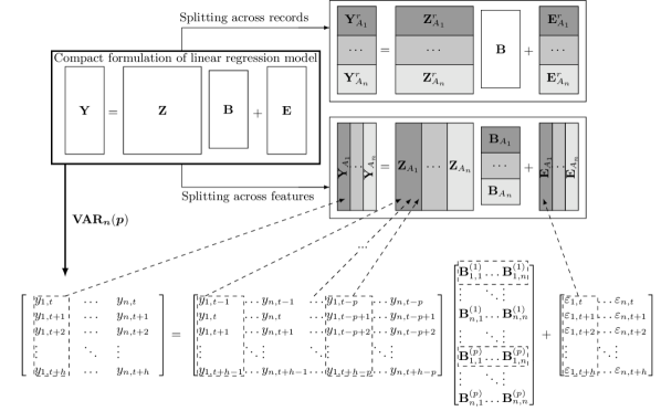
Figure 2: Common data division structures and VAR model.

$\overbrace{\rule{42.67912pt}{0.0pt}}^{\text{Y of i-th data owner}}$	$\overbrace{\rule{182.09746pt}{0.0pt}}^{\text{covariates values of i-th data owner}}$
$y_{i,t}$	$y_{i,t-1}$	$y_{i,t-2}$	$y_{t-3,i}$	$\dots$	$y_{i,t-p+1}$	$y_{i,t-p}$
$y_{i,t+1}$	$y_{i,t}$	$y_{i,t-1}$	$y_{t-2,i}$	$\dots$	$y_{i,t-p+2}$	$y_{i,t-p+1}$
$y_{i,t+2}$	$y_{i,t+1}$	$y_{i,t}$	$y_{t-1,i}$	$\dots$	$y_{i,t-p+3}$	$y_{i,t-p+2}$
⋮	⋮	⋮	⋮	⋮	⋮	⋮
$y_{i,t+h}$	$y_{i,t+h-1}$	$y_{i,t+h-2}$	$y_{t+h-3,i}$	$\dots$	$y_{i,t+h-p+1}$	$y_{i,t+h-p}$

Figure 3: Illustration of the data used by the $i$-th data owner when fitting a VAR model.

3.2 Estimation in VAR Models

Commonly, when the number of covariates included, $np$, is substantially smaller than the length of the time series, $T$, the VAR model can be fitted using multivariate least squares solution given by

$$\hat{\mathbf{B}}_{\text{LS}}=\operatorname*{argmin}_{\mathbf{B}}\left(\|\mathbf{Y}-\mathbf{ZB}\|_{2}^{2}\right)\ ,$$ (39)

where $\|.\|_{r}$ represents both vector and matrix $L_{r}$ norms. However, in collaborative forecasting, as the number of data owners increases, as well as the number of lags, it becomes crucial to use regularization techniques, such as LASSO, in order to introduce sparsity into the coefficient matrix estimated by the model. In the standard LASSO-VAR approach (see Nicholson et al. [2017] for different variants of the LASSO regularization in the VAR model), the coefficients are given by

$$\hat{\mathbf{B}}=\operatorname*{argmin}_{\mathbf{B}}\left(\frac{1}{2}\|\mathbf{Y}-\mathbf{ZB}\|_{2}^{2}+\lambda\|\mathbf{B}\|_{1}\right),$$ (40)

where $\lambda>0$ is a scalar penalty parameter.

With the addition of the LASSO regularization term, the convex objective function in (40) becomes non-differentiable, thus limiting the variety of optimization techniques that can be employed. In this domain, ADMM (which was described in 2.3.1) is a widespread and computationally efficient technique that enables the parallel estimation for data divided by features. The ADMM formulation of the non-differentiable cost function associated to LASSO-VAR model in (40) solves the optimization problem

$$\min_{\mathbf{B},\mathbf{H}}\Big{(}\frac{1}{2}\|\mathbf{Y}-\mathbf{ZB}\|_{2}^{2}+\lambda\|\mathbf{H}\|_{1}\Big{)}\text{ subject to }\mathbf{H}=\mathbf{B}\ ,$$ (41)

which differs from (40) by splitting $\mathbf{B}$ into two parts ($\mathbf{B}$ and $\mathbf{H}$). This allows splitting the objective function in two distinct objective functions, $f(\mathbf{B})=\frac{1}{2}\|\mathbf{Y}-\mathbf{ZB}\|_{2}^{2}$ and $g(\mathbf{H})=\lambda\|\mathbf{H}\|_{1}$. The augmented Lagrangian [Boyd et al., 2011] of this problem is

$$L_{\rho}(\mathbf{B},\mathbf{H},\mathbf{W})=\frac{1}{2}\|\mathbf{Y}-\mathbf{ZB}\|_{2}^{2}+\lambda\|\mathbf{H}\|_{1}+\mathbf{W}^{\top}(\mathbf{B}-\mathbf{H})+\frac{\rho}{2}\|\mathbf{B}-\mathbf{H}\|_{2}^{2}\ ,$$ (42)

where $\mathbf{W}$ is the dual variable and $\rho>0$ is the penalty parameter. The scaled form of this Lagrangian is

$$L_{\rho}(\mathbf{B},\mathbf{H},\mathbf{U})=\frac{1}{2}\|\mathbf{Y}-\mathbf{ZB}\|_{2}^{2}+\lambda\|\mathbf{H}\|_{1}+\frac{\rho}{2}\|\mathbf{B}-\mathbf{H}+\mathbf{U}\|^{2}-\frac{\rho}{2}\|\mathbf{U}\|^{2}\ ,$$ (43)

where $\mathbf{U}=(1/\rho)\mathbf{W}$ is the scaled dual variable associated with the constrain $\mathbf{B}=\mathbf{H}$. Hence, according to (29), the ADMM formulation for LASSO-VAR consists in the following iterations [Cavalcante et al., 2017],

$$\left\{\begin{array}[]{l}\displaystyle\mathbf{B}^{k+1}:=\operatorname*{argmin}_{\mathbf{B}}\Big{(}\frac{1}{2}\|\mathbf{Y-ZB}\|_{2}^{2}+\frac{\rho}{2}\|\mathbf{B}-\mathbf{H}^{k}+\mathbf{U}^{k}\|_{2}^{2}\Big{)}\\ \displaystyle\mathbf{H}^{k+1}:=\operatorname*{argmin}_{\mathbf{H}}\Big{(}\lambda\|\mathbf{H}\|_{1}+\frac{\rho}{2}\|\mathbf{B}^{k+1}-\mathbf{H}+\mathbf{U}^{k}\|_{2}^{2}\Big{)}\\ \mathbf{U}^{k+1}:=\mathbf{U}^{k}+\mathbf{B}^{k+1}-\mathbf{H}^{k+1}.\end{array}\right.$$ (44)

Concerning the LASSO-VAR model, and since data is naturally divided by features (i.e. $\mathbf{Y}=\allowbreak[\mathbf{Y}_{A_{1}},\allowbreak\dots,\allowbreak\mathbf{Y}_{A_{n}}]$, $\mathbf{Z}=\allowbreak[\mathbf{Z}_{A_{1}},\allowbreak\dots,\allowbreak\mathbf{Z}_{A_{n}}]$ and $\mathbf{B}=[\mathbf{B}^{\top}_{A_{1}},\dots,\mathbf{B}^{\top}_{A_{n}}]^{\top}$) and the functions $\|\mathbf{Y-ZB}\|_{2}^{2}$ and $\|\mathbf{B}\|_{1}$ are decomposable (i.e. $\|\mathbf{Y-ZB}\|_{2}^{2}=\|\mathbf{Y}-\sum_{i=1}^{n}\mathbf{Z}_{A_{i}}\mathbf{B}_{A_{i}}\|_{2}^{2}$ and $\|\mathbf{B}\|_{1}=\sum_{i=1}^{n}\mathbf{\|}\mathbf{B}_{A_{i}}\|_{1}$), the model fitting problem (40) becomes

$$\operatorname*{argmin}_{\boldsymbol{\Gamma}}\left(\frac{1}{2}\|\mathbf{Y}-\sum_{i=1}^{n}\mathbf{Z}_{A_{i}}\mathbf{B}_{A_{i}}\|_{2}^{2}+\lambda\sum_{i=1}^{n}\|\mathbf{B}_{A_{i}}\|_{1}\right),$$ (45)

$\boldsymbol{\Gamma}=\{\mathbf{B}_{A_{1}},\dots,\mathbf{B}_{A_{n}}\}$, which is rewritten as

$$\operatorname*{argmin}_{\boldsymbol{\Gamma}^{\prime}}\left(\frac{1}{2}\|\mathbf{Y}-\sum_{i=1}^{n}\mathbf{H}_{A_{i}}\|_{2}^{2}+\lambda\sum_{i=1}^{n}\|\mathbf{B}_{A_{i}}\|_{1}\right)\text{ s.t. }{\mathbf{B}_{A_{1}}\mathbf{Z}_{A_{1}}=\mathbf{H}_{A_{1}},\ \dots,\ \mathbf{B}_{A_{n}}\mathbf{Z}_{A_{n}}=\mathbf{H}_{A_{n}}\ ,}$$ (46)

$\boldsymbol{\Gamma}^{\prime}=\{\mathbf{B}_{A_{1}},\dots,\mathbf{B}_{A_{n}},\mathbf{H}_{A_{1}},\dots,\mathbf{H}_{A_{n}}\}$, while the corresponding distributed ADMM formulation [Boyd et al., 2011, Cavalcante et al., 2017] is the one presented in the system of equations (47),

$$\mathbf{B}_{A_{i}}^{k+1}=\operatorname*{argmin}_{\mathbf{B}_{A_{i}}}\left(\frac{\rho}{2}\|\mathbf{Z}_{A_{i}}\mathbf{B}_{A_{i}}^{k}+\overline{\mathbf{H}}^{k}-\overline{\mathbf{ZB}}^{k}-\mathbf{U}^{k}-\mathbf{Z}_{A_{i}}\mathbf{B}_{A_{i}}\|_{2}^{2}+\lambda\|\mathbf{B}_{A_{i}}\|_{1}\right),$$ (47a)

$$\overline{\mathbf{H}}^{k+1}=\frac{1}{N+\rho}\left(\mathbf{Y}+\rho\overline{\mathbf{ZB}}^{k+1}+\rho\mathbf{U}^{k}\right),$$ (47b)

$$\mathbf{U}^{k+1}=\mathbf{U}^{k}+\overline{\mathbf{ZB}}^{k+1}-\overline{\mathbf{H}}^{k+1},$$ (47c)

where $\overline{\mathbf{ZB}}^{k+1}=\frac{1}{n}\sum_{j=1}^{n}\mathbf{Z}_{A_{j}}\mathbf{B}^{k+1}_{A_{j}}$ and $\mathbf{B}_{A_{i}}^{k+1}\in\mathbb{R}^{p\times n}$, $\mathbf{Z}_{A_{i}}\in\mathbb{R}^{T\times p}$,$\mathbf{Y}\in\mathbb{R}^{T\times n}$, $\overline{\mathbf{H}}^{k},\mathbf{U}\in\mathbb{R}^{T\times n}$, $i=1,...,n$.

Although the parallel computation is an appealing property for the design of a privacy-preserving approach, ADMM is an iterative optimization process that requires intermediate calculations, thus a careful analysis is necessary to evaluate if some confidentiality breaches can occur at the end of some iterations.

3.3 Privacy Analysis

3.3.1 Data Transformation with Noise Addition

This section presents experiments with simulated data and solar energy data collected from a smart grid pilot in Portugal. The objective is to quantify the impact of data distortion (through noise addition) into the model forecasting skill.

a) Synthetic Data: An experiment has been performed to add random noise from the Gaussian distribution with zero mean and variance $b^{2}$, Laplace distribution with zero mean and scale parameter $b$ and Uniform distribution with support $[-b,b]$, represented by $\mathcal{N}(0,b^{2})$, $\mathcal{L}(0,b)$ and $\mathcal{U}(-b,b)$, respectively. Synthetic data generated by VAR processes are used to measure the differences between the coefficients’ values when adding noise to the data. The simplest case considers a VAR with two data owners and two lags described by

$$\left(\begin{matrix}y_{1,t}\ y_{2,t}\\ \end{matrix}\right){=}\left(\begin{matrix}y_{1,t-1}\ y_{2,t-1}\ y_{1,t-2}\ y_{2,t-2}\\ \end{matrix}\right)\left(\begin{matrix}0.5&0.3\\ 0.3&0.75\\ -0.3&-0.05\\ -0.1&-0.4\\ \end{matrix}\right){+}\left(\begin{matrix}\varepsilon_{1,t}\ \varepsilon_{2,t}\\ \end{matrix}\right).$$

The second case includes ten data owners and three lags, introducing a high percentage of null coefficients ($\approx 86\%$), with Figure 4 illustrating the considered coefficients. Since a specific configuration can generate various distinct trajectories, 100 simulations are performed for each specified VAR model, each of them with 20,000 timestamps. For both simulated datasets, the errors $\boldsymbol{\varepsilon}_{t}$ were assumed to follow a multivariate Normal distribution with a zero mean vector and a covariance matrix equal to the identity matrix of appropriate dimensions. Distributed ADMM (detailed in Section 2.3.1) was used to estimate the LASSO-VAR coefficients, considering two different noise characterizations, $b\in\{0.2,0.6\}$.

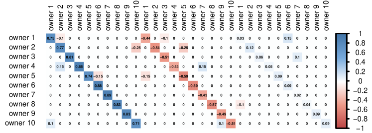
Figure 4: Transpose of the coefficient matrix used to generate the VAR with 10 data owners and 3 lags.

Figure 5 summarizes the mean and the standard deviation of the absolute difference between the real and estimated coefficients, for both VAR processes, from 100 simulations. The greater the noise $b$, the greater the distortion of the estimated coefficients. Moreover, the Laplace distribution, which has desirable properties to make the data private according to the differential privacy framework, registers the greater distortion in the estimated model.

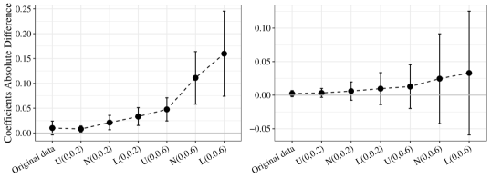
Figure 5: Mean $\pm$ standard deviation for the absolute difference between the real and estimated coefficients (left: VAR with 2 data owners, right: VAR with 10 data owners).

Using the original data, the ADMM solution tends to stabilize after 50 iterations, and the value of the coefficients is correctly estimated (the difference is approximately zero). Regarding the distorted time series, it converges faster, but the coefficients deviate from the real ones. In fact, adding noise contributes to decreasing the absolute value of the coefficients, i.e. the relationships between the time series become weakened.

These experiments allow drawing some conclusions about the use of differential privacy. The Laplace distribution has advantageous properties, since it ensures $\varepsilon$-differential privacy when random noise follows $\mathcal{L}(0,\frac{\Delta f_{1}}{\varepsilon})$. For the VAR with two data owners, $\Delta f_{1}\approx 12$ since the observed values are in the interval $[-6,6]$. Therefore, $\varepsilon=20$ when $\mathcal{L}(0,0.6)$ and $\varepsilon=15$ when $\mathcal{L}(0,0.8)$, meaning that the data still encompass much relevant information. Finally, to verify the impact of noise addition into forecasting performance, Figure 7 illustrates the improvement of each estimated VAR${}_{2}(2)$ model (with and without noise addition) over the Autoregressive (AR) model estimated with original time series, in which collaboration is not used. This improvement is measured in terms of Mean Absolute Error (MAE) and Root Mean Squared Error (RMSE) values. Concerning the case with ten data owners, and when using data without noise, seven data owners improve their forecasting performance, which was expected from the coefficient matrix in Figure 4. When Laplacian noise is applied to the data, only one data owner (the first one) improves its forecasting skill (when compared to the AR model) by using the estimated VAR model. Even though the masked data continues to provide relevant information, the model obtained for the Laplacian noise performs worse than the AR model for the second data owner, making the VAR useless for the majority of the data owners.

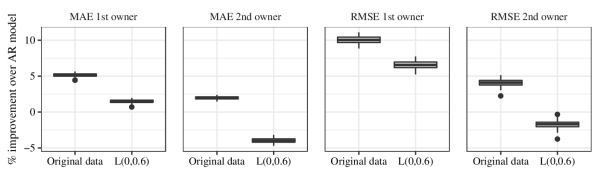
Figure 6: Improvement (%) of VAR${}_{2}(2)$ model over AR(2) model, in terms of MAE and RMSE for synthetic data.

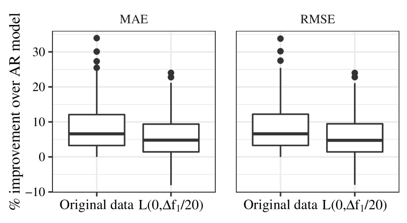
(a) VAR${}_{2}(2)$ model.

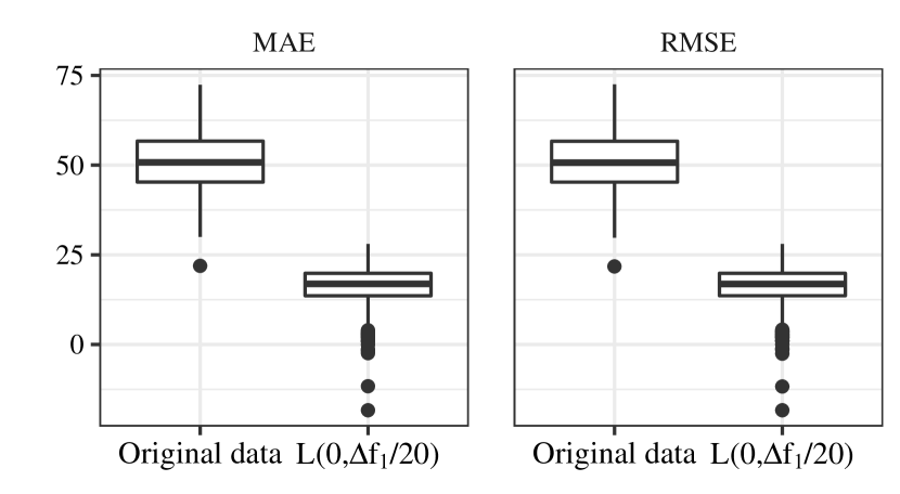
(b) VAR${}_{10}(3)$ model.

Figure 7: Improvement (%) of VAR model over AR model, in terms of MAE and RMSE for synthetic data.

However, the results cannot be generalized for all VAR models, especially regarding the illustrated VAR${}_{10}(3)$, which is very close to the AR(3) model. Given that, a third experiment is proposed, in which 200 random coefficient matrices are generated for a stationary VAR${}_{2}(2)$ and VAR${}_{10}(3)$ following the algorithm proposed by Ansley & Kohn [1986]. Usually, the generated coefficient matrix has no null entries and the higher values are not necessarily found on diagonals. Figure 7 illustrates the improvement for each data owner when using a VAR model (with and without noise addition) over the AR model. In this case, the percentage of times the AR model performs better than the VAR model with distorted data is smaller, but the degradation of the models is still noticeable, especially in relation to the case with 10 data owners.

b) Real Data: The real dataset encompasses hourly time series of solar power generation from 44 micro-generation units located in Évora city (Portugal), covering the period from February 1, 2011 to March 6, 2013. As in Cavalcante & Bessa [2017], records corresponding to a solar zenith angle higher than 90^∘ were removed, in order to take off nighttime hours (i.e., hours without any generation). Furthermore, and to make the time series stationary, a normalization of the solar power was applied by using a clear-sky model (see Bacher et al. [2009]) that gives an estimate of the solar power in clear sky conditions at any given time. The power generation for the next hour is modeled through the VAR model, which combines data from 44 data owners and considers 3 non-consecutive lags (1, 2 and 24h). Figure 8 (a) summarizes the improvement for the 44 PV power plants over the autoregressive model, in terms of MAE and RMSE. The quartile 25% allows concluding that MAE improves at least 10% for 33 of the 44 PV power plants, when data owners share their observed data. As to RMSE the improvement is not so significant, but is still greater than zero. Although the data obtained after Laplacian noise addition keeps its temporal dependency, as illustrated in Figure 8 (b), the corresponding VAR model is useless for 4 of the 44 data owners. When considering RMSE, 2 of the 44 data owners obtain better results by using an autoregressive model. Once again, the resulting model suffers a significant reduction in terms of forecasting capability.

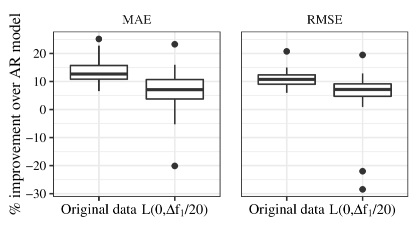
(a) Improvement (%) of VAR₄₄ model over AR model, in terms of MAE and RMSE.

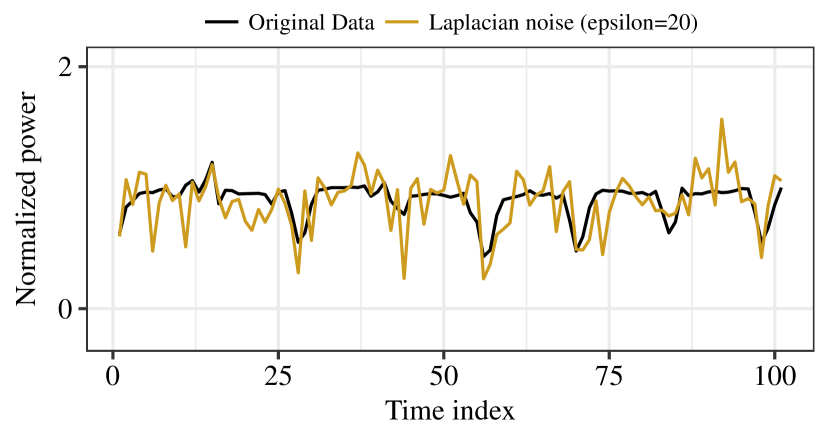
(b) Example of the normalized time series.

Figure 8: Results for real case-study with solar power time series.

3.3.2 Linear Algebra-based Protocols

Let us consider the case with two data owners. Since the multivariate least squares estimate for the VAR model with covariates $\mathbf{Z}=[\mathbf{Z}_{A_{1}},\mathbf{Z}_{A_{2}}]$ and target $\mathbf{Y}=[\mathbf{Y}_{A_{1}},\mathbf{Y}_{A_{2}}]$ is

$$\hat{\mathbf{B}}_{\text{LS}} =\left(\left[\begin{tabular}[]{c}$\mathbf{Z}^{\top}_{A_{1}}$\\ $\mathbf{Z}^{\top}_{A_{2}}$\\ \end{tabular}\right][\mathbf{Z}_{A_{1}},\mathbf{Z}_{A_{2}}]\right)^{-1}\left(\left[\begin{tabular}[]{c}$\mathbf{Z}^{\top}_{A_{1}}$\\ $\mathbf{Z}^{\top}_{A_{2}}$\\ \end{tabular}\right][\mathbf{Y}_{A_{1}},\mathbf{Y}_{A_{2}}]\right)$$ (52)

$$=\left(\begin{tabular}[]{cc}$\mathbf{Z}^{\top}_{A_{1}}\mathbf{Z}_{A_{1}}$&$\mathbf{Z}^{\top}_{A_{1}}\mathbf{Z}_{A_{2}}$\\ $\mathbf{Z}^{\top}_{A_{2}}\mathbf{Z}_{A_{1}}$&$\mathbf{Z}^{\top}_{A_{2}}\mathbf{Z}_{A_{2}}$\\ \end{tabular}\right)^{-1}\left(\begin{tabular}[]{cc}$\mathbf{Z}^{\top}_{A_{1}}\mathbf{Y}_{A_{1}}$&$\mathbf{Z}^{\top}_{A_{1}}\mathbf{Y}_{A_{2}}$\\ $\mathbf{Z}^{\top}_{A_{2}}\mathbf{Y}_{A_{1}}$&$\mathbf{Z}^{\top}_{A_{2}}\mathbf{Y}_{A_{2}}$\\ \end{tabular}\right),$$ (57)

the data owners need to jointly compute $\mathbf{Z}_{A_{1}}^{\top}\mathbf{Z}_{A_{2}}$, $\mathbf{Z}_{A_{1}}^{\top}\mathbf{Y}_{A_{2}}$ and $\mathbf{Z}_{A_{2}}^{\top}\mathbf{Y}_{A_{1}}$.

As mentioned in the introduction of Section 2.2.1, the work of Du et al. [2004] proposes protocols for secure matrix multiplication for the situations where two data owners observe the same common target matrix and different confidential covariates. Unfortunately, without assuming a trusted third entity for generating random matrices, the proposed protocol fails when applied to the VAR model because $2(T-1)p$ values of the covariate matrix $\mathbf{Z}\in\mathbb{R}^{T\times 2p}$ are included in the target matrix $\mathbf{Y}\in\mathbb{R}^{T\times 2}$, which is also undisclosed. Additionally, $\mathbf{Z}_{A_{i}}\in\mathbb{R}^{T\times p}$ has $T+p-1$ unique values instead of $Tp$ – see Figure 3.

Proposition 1

Consider the case in which two data owners, with private data $\mathbf{Z}_{A_{i}}\in\mathbb{R}^{T\times p}$ and $\mathbf{Y}_{A_{i}}\in\mathbb{R}^{T\times 1}$, want to estimate a VAR model without trusting a third entity, $i=1,2$. Assume that the $T$ records are consecutive, as well as the $p$ lags. The multivariate least squares estimate for the VAR model with covariates $\mathbf{Z}=[\mathbf{Z}_{A_{1}},\mathbf{Z}_{A_{2}}]$ and target $\mathbf{Y}=[\mathbf{Y}_{A_{1}},\mathbf{Y}_{A_{2}}]$ requires the computation of $\mathbf{Z}_{A_{1}}^{\top}\mathbf{Z}_{A_{2}}$, $\mathbf{Z}_{A_{1}}^{\top}\mathbf{Y}_{A_{2}}$ and $\mathbf{Z}_{A_{2}}^{\top}\mathbf{Y}_{A_{1}}$.

If data owners use the protocol proposed by Du et al. [2004] for computing such matrices, then the information exchanged allows to recover data matrices.

Proof 1

As in Du et al. [2004], let us consider the case with two data owners without a third entity generating random matrices.

In order to compute $\mathbf{Z}_{A_{1}}^{\top}\mathbf{Z}_{A_{2}}$ both data owners define a matrix $\mathbf{M}\in\mathbb{R}^{T\times T}$ and compute its inverse $\mathbf{M}^{-1}$. Then, the protocol defines that

$$\mathbf{Z}_{A_{1}}^{\top}\mathbf{Z}_{A_{2}} =\mathbf{Z}_{A_{1}}^{\top}\mathbf{MM^{-1}}\mathbf{Z}_{A_{2}}=\mathbf{A}[\mathbf{M}_{\text{left}},\mathbf{M}_{\text{right}}]\left[\begin{tabular}[]{l}$(\mathbf{M}^{-1})_{\text{top}}$\\ $(\mathbf{M}^{-1})_{\text{bottom}}$\end{tabular}\right]\mathbf{Z}_{A_{2}}$$

$$=\underbrace{\mathbf{Z}_{A_{1}}^{\top}\mathbf{M}_{\text{left}}(\mathbf{M}^{-1})_{\text{top}}\mathbf{Z}_{A_{2}}}_{\text{derived by Owner~{}\#1}}+\underbrace{\mathbf{Z}_{A_{1}}^{\top}\mathbf{M}_{\text{right}}(\mathbf{M}^{-1})_{\text{bottom}}\mathbf{Z}_{A_{2}}}_{\text{derived by Owner~{}\#2}}\ ,$$

requiring data owners to share $\mathbf{Z}^{\top}_{A_{1}}\mathbf{M}_{\text{right}}\in\mathbb{R}^{p\times T/2}$ and $(\mathbf{M}^{-1})_{\text{top}}\mathbf{Z}_{A_{2}}\in\mathbb{R}^{T/2\times p}$, respectively. This implies that each data owner shares $pT/2$ values.

Similarly, the computation of $\mathbf{Z}_{A_{1}}^{\top}\mathbf{Y}_{A_{2}}$ implies that data owners define a matrix $\mathbf{M}^{*}$, and share $\mathbf{Z}^{\top}_{A_{1}}\mathbf{M}^{*}_{\text{right}}\in\mathbb{R}^{p\times T/2}$ and $(\mathbf{M^{*}}^{-1})_{\text{top}}\mathbf{Y}_{A_{2}}\in\mathbb{R}^{T/2\times p}$, respectively, providing new $pT/2$ values. This means that Owner #2 receives $\mathbf{Z}^{\top}_{A_{1}}\mathbf{M}_{\text{right}}$ and $\mathbf{Z}^{\top}_{A_{1}}\mathbf{M}^{*}_{\text{right}}$, i.e. $Tp$ values, and may recover $\mathbf{Z}_{A_{1}}$ which consists of $Tp$ values, representing a confidentiality breach. Furthermore, when considering a VAR model with $p$ lags, $\mathbf{Z}_{A_{1}}$ has $T+p-1$ unique values, meaning less values to recover. Analogously, Owner #1 may recover $\mathbf{Z}_{A_{2}}$ through the matrices shared for the computation of $\mathbf{Z}_{A_{1}}^{\top}\mathbf{Z}_{A_{2}}$ and $\mathbf{Z}_{A_{2}}^{\top}\mathbf{Y}_{A_{1}}$.

Lastly, when considering a VAR with $p$ lags, $\mathbf{Y}_{A_{i}}$ only has $p$ values that are not in $\mathbf{Z}_{A_{i}}$. Since, while computing $\mathbf{Z}_{A_{1}}^{\top}\mathbf{Y}_{A_{2}}$, Owner #1 receives $T/2$ values from $(\mathbf{M}*^{-1})_{\text{top}}\mathbf{Y}_{A_{2}}\in\mathbb{R}^{T/2\times 1}$, a confidentiality breach can occur (in general $T/2>p$). In the same way, Owner #2 recovers $\mathbf{Y}_{A_{1}}$ when computing $\mathbf{Z}_{A_{2}}^{\top}\mathbf{Y}_{A_{1}}$.

The main disadvantage of the linear algebra-based methods is that they do not take into account that, in the VAR model, both target variables and covariates are private and that a large proportion of the covariates matrix is determined by knowing the target variables. This means that the data shared between data owners may be enough for competitors to be able to reconstruct the original data. For the method proposed by Karr et al. [2009], a consequence of such data is that the assumption $rank\left(\mathbf{(I-WW^{\top})}\allowbreak\mathbf{C}\right)=m{-}g$ may still provide a number of linearly independent equations on the other data owner’s data, which is enough for recovering their data.

3.3.3 ADMM Method and Central Node

The work of Zhang & Wang [2018] appears to be a promising approach for dealing with the problem of private data during the ADMM iterative process described by (47). Based on Zhang & Wang [2018], for each iteration $k$, each data owner $i$ communicates their local results, $\mathbf{Z}_{A_{i}}\mathbf{B}^{k+1}_{A_{i}}$, to the central node, $\mathbf{Z}_{A_{i}}\in\mathbb{R}^{T\times p},\mathbf{B}^{k+1}_{A_{i}}\in\mathbb{R}^{p\times n},i=1,\dots,n$. Then, the central node computes the intermediate matrices in (47b)-(47c) and returns the matrix $\overline{\mathbf{H}}^{k}-\overline{\mathbf{ZB}}^{k}-\mathbf{U}^{k}$ to each data owner, in order to update $\mathbf{B}_{A_{i}}$ in the next iteration, as seen in (47a). Figure 9 illustrates the methodology for the LASSO-VAR with three data owners. In this solution, there is no direct exchange of private data. However, as presented next, not only can the central node recover the original data, but also individual data owners can obtain a good estimation of the data used by the competitors.

Proposition 2

In the most optimistic scenario, without repeated values in $\mathbf{Y}_{A_{i}}\in\mathbb{R}^{T\times 1}$ and $\mathbf{Z}_{A_{i}}\in\mathbb{R}^{T\times p}$, when applying the algorithm from Zhang et al. [2019] to solve the LASSO-VAR model in (47), the central agent can recover the sensible data at the end of

$$k=\bigg{\lceil}\frac{Tp}{Tn-pn}\bigg{\rceil}$$ (58)

iterations, where $\lceil x\rceil$ denotes the ceiling function.

Figure 9: Distributed ADMM LASSO-VAR with a central node and 3 data owners (related to the algorithm in (47)).

Proof 2

Using the notation of Section 3.1, each of the $n$ data owners is assumed to use the same number of lags $p$ to fit a LASSO-VAR model with a total number of $T$ records (keep in mind that $T>np$, otherwise there will be more coefficients to be determined than system equations). At the end of $k$ iterations, the central node receives a total of $Tnk$ values from each data owner $i$, corresponding to $\mathbf{Z}_{A_{i}}\mathbf{B}_{A_{i}}^{1},\mathbf{Z}_{A_{i}}\mathbf{B}_{A_{i}}^{2},...,\mathbf{Z}_{A_{i}}\mathbf{B}_{A_{i}}^{k}{\in\mathbb{R}^{T\times n}}$, and does not know $pnk+Tp$, corresponding to $\mathbf{B}_{A_{i}}^{1},...,\mathbf{B}_{A_{i}}^{k}{\in\mathbb{R}^{p\times n}}$ and $\mathbf{Z}_{A_{i}}{\in\mathbb{R}^{T\times p}}$, respectively, $i=1,...,n$. Given that, the solution of the inequality

$$Tnk\geq pnk+Tp\ ,$$ (59)

in $k$, allows to infer that a confidentiality breach can occur at the end of

$$k=\bigg{\lceil}\frac{Tp}{Tn-pn}\bigg{\rceil}$$ (60)

iterations, where $\lceil x\rceil$ denotes the ceiling function. Since $T$ tends to be large, $k$ tends to $\lceil p/n\rceil$, which may represent a confidentiality breach if the number of iterations required for the algorithm to converge is greater than $\lceil p/n\rceil$.

Proposition 3

In the most optimistic scenario, without repeated values in $\mathbf{Y}_{A_{i}}\in\mathbb{R}^{T\times 1}$ and $\mathbf{Z}_{A_{i}}\in\mathbb{R}^{T\times p}$, when applying the algorithm from Zhang et al. [2019] to solve the LASSO-VAR model in (47), the data owners can recover the sensible data from competitors at the end of

$$k=\bigg{\lceil}\frac{Tn+(n-1)(Tp+T)}{Tn-(n-1)pn}\bigg{\rceil}$$ (61)

iterations.

Proof 3

Without loss of generality, Owner #1 is considered the semi-trusted data owner — a semi-trusted data owner completes and shares his/her computations faithfully, but tries to learn additional information while or after the algorithm runs. For each iteration $k$, this data owner receives the intermediate matrix $\overline{\mathbf{H}}^{k}-\underbrace{\overline{\mathbf{ZB}}^{k}}_{=\frac{1}{n}\sum_{i=1}^{n}\mathbf{Z}_{A_{i}}\mathbf{B}_{A_{i}}^{k}}-\mathbf{U}^{k}{\in\mathbb{R}^{T\times n}}$, which provides $Tn$ values. However, Owner #1 does not know

$$\underbrace{-\mathbf{U}^{k}+\overline{\mathbf{H}}^{k}}_{\in\mathbb{R}^{T\times n}},\underbrace{\mathbf{B}_{A_{2}}^{k},\dots,\mathbf{B}_{A_{n}}^{k}}_{\text{$n-1$ matrices $\in\mathbb{R}^{p\times n}$}},\underbrace{\mathbf{Z}_{A_{2}},\dots,\mathbf{Z}_{A_{n}}}_{\text{$n-1$ matrices $\in\mathbb{R}^{T\times p}$}},\underbrace{\mathbf{Y}_{A_{2}},\dots,\mathbf{Y}_{A_{n}}}_{\text{$n-1$ matrices $\in\mathbb{R}^{T\times 1}$}},$$

which corresponds to $Tn+(n-1)pn+(n-1)Tp+(n-1)T$ values. However, since all the data owners know that $\overline{\mathbf{H}}^{k}$ and $\mathbf{U}^{k}$ are defined by the expressions in (47b) and (47c), it is possible to perform some simplifications in which $\mathbf{U}^{k}$ and $\overline{\mathbf{H}}^{k}-\overline{\mathbf{ZB}}^{k}-\mathbf{U}^{k}$ becomes (62) and (63), respectively,

$$\begin{split}\mathbf{U}^{k}\stackrel{{\scriptstyle\eqref{eq:admmcolumnC}}}{{=}}&\mathbf{U}^{k-1}+\overline{\mathbf{ZB}}^{k}-\overline{\mathbf{H}}^{k}=\mathbf{U}^{k-1}+\overline{\mathbf{ZB}}^{k}-\underbrace{\frac{1}{N+\rho}\left(\mathbf{Y}+\rho\overline{\mathbf{ZB}}^{k}+\rho\mathbf{U}^{k-1}\right)}_{\text{$=\overline{\mathbf{H}}^{k}$, according to~{}\eqref{eq:admmcolumnB}}}\\ =&\Big{[}1-\frac{\rho}{N+\rho}\Big{]}\mathbf{U}^{k-1}+\Big{[}1-\frac{\rho}{N+\rho}\Big{]}\overline{\mathbf{ZB}}^{k}-\frac{1}{N+\rho}\mathbf{Y}\ ,\end{split}$$ (62)

$$\begin{split}\overline{\mathbf{H}}^{k}{-}\overline{\mathbf{ZB}}^{k}{-}\mathbf{U}^{k}&{=}\underbrace{\frac{1}{N+\rho}\left(\mathbf{Y}+\rho\overline{\mathbf{ZB}}^{k}+\rho\mathbf{U}^{k-1}\right)}_{\text{=$\overline{\mathbf{H}}^{k}$, according to~{}\eqref{eq:admmcolumnB}}}-\overline{\mathbf{ZB}}^{k}-\mathbf{U}^{k}.\end{split}$$ (63)

Therefore, the iterative process to find the competitors’ data proceeds as follows:

1. Initialization: The central node generates $\mathbf{U}^{0}\in\mathbb{R}^{T\times n}$, and the $i$-th data owner generates $\mathbf{B}_{A_{i}}^{1}\in\mathbb{R}^{p\times n}$, $i\in\{1,...,n\}$.

2. Iteration #1: The central node receives $\mathbf{Z}_{A_{i}}\mathbf{B}_{A_{i}}^{1}$ and computes $\mathbf{U}^{1}$, returning $\overline{\mathbf{H}}^{1}-\overline{\mathbf{ZB}}^{1}-\mathbf{U}^{1}\in\mathbb{R}^{T\times n}$ which is returned for all $n$ data owners. At this point, Owner #1 receives $Tn$ values and does not know

   $$\underbrace{\mathbf{U}^{0}}_{\in\mathbb{R}^{T\times n}},\underbrace{\mathbf{B}_{A_{2}}^{1},...,\mathbf{B}_{A_{n}}^{1}}_{\text{$n-1$ matrices $\in\mathbb{R}^{p\times n}$}},\underbrace{\mathbf{Z}_{A_{2}},...,\mathbf{Z}_{A_{n}}}_{\text{$n-1$ matrices $\in\mathbb{R}^{T\times p}$}}\ ,$$

   and $n{-}1$ columns of $\mathbf{Y}\in\mathbb{R}^{T\times n}$, corresponding to $Tn+(n-1)[pn+Tp+T]$ values.

3. Iteration #2: The central node receives $\mathbf{Z}_{A_{i}}\mathbf{B}_{A_{i}}^{2}$ and computes $\mathbf{U}^{2}$, returning $\overline{\mathbf{H}}^{2}-\overline{\mathbf{ZB}}^{2}-\mathbf{U}^{2}$ for the $n$ data owners. At this point, only new estimations for the vectors $\mathbf{B}_{A_{2}},...,\mathbf{B}_{A_{n}}$ were introduced in the system, which means more $(n{-}1)pn$ values to estimate.

As a result, at the end of $k$ iterations, Owner #1 has received $\mathbf{Z}_{A_{i}}\mathbf{B}_{A_{i}}^{1},\dots,\mathbf{Z}_{A_{i}}\mathbf{B}_{A_{i}}^{k}\in\mathbb{R}^{T\times n}$ corresponding to $Tnk$ values and needs to estimate

$$\underbrace{\mathbf{U}^{0}}_{\in\mathbb{R}^{T\times n}},\underbrace{\mathbf{B}_{A_{2}}^{1},...,\mathbf{B}_{A_{n}}^{1},\mathbf{B}_{A_{2}}^{2},...,\mathbf{B}_{A_{n}}^{2},\dots,\mathbf{B}_{A_{2}}^{k},...,\mathbf{B}_{A_{n}}^{k}}_{\text{$(n-1)k$ matrices $\in\mathbb{R}^{p\times n}$}},\underbrace{\mathbf{Z}_{A_{2}},...,\mathbf{Z}_{A_{n}}}_{\text{$n-1$ matrices $\in\mathbb{R}^{T\times p}$}}\ ,$$

and $n{-}1$ columns of $\mathbf{Y}\in\mathbb{R}^{T\times n}$, corresponding to $Tn{+}(n{-}1)[kpn{+}Tp{+}T]$. Then, the solution for the inequality

$$Tnk\geq Tn+(n-1)[kpn+Tp+T]{\ ,}$$ (64)

allows to infer that a confidentiality breach may occur at the end of

$$k=\bigg{\lceil}\frac{Tn+(n-1)(Tp+T)}{Tn-(n-1)pn}\bigg{\rceil}$$ (65)

iterations.

Figure 10 illustrates the $k$ value for different combinations of $T$, $n$, and $p$. In general, the greater the number of records $T$, the smaller the number of iterations necessary for confidentiality breach. That is because more information is shared during each iteration of the ADMM algorithm. On the other hand, the number of iterations until a possible confidentiality breach increases with the number of data owners ($n$). The same is true for the number of lags ($p$).

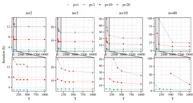
Figure 10: Number of iterations until a possible confidentiality breach, considering the centralized ADMM-based algorithm in [Zhang et al., 2019].

3.3.4 ADMM Method and Noise Mechanisms

The target matrix $\mathbf{Y}=[\mathbf{Y}_{A_{1}},\dots,\mathbf{Y}_{A_{n}}]$ corresponds to the sum of private matrices $\mathbf{I}_{\mathbf{Y}_{A_{i}}}\in\mathbb{R}^{T\times n}$, i.e.

$$\underbrace{\left[\begin{tabular}[]{lllll}$y_{1,t}$&$y_{2,t}$&\ldots&$y_{n,t}$\\ $y_{1,t+1}$&$y_{2,t+1}$&\ldots&$y_{n,t+1}$\\ $y_{1,t+2}$&$y_{2,t+2}$&\ldots&$y_{n,t+2}$\\ \vdots&$\ddots$&\vdots\\ $y_{1,t+h}$&$y_{2,t+h}$&\ldots&$y_{n,t+h}$\\ \end{tabular}\right]}_{\mathbf{Y}}=\underbrace{\left[\begin{tabular}[]{lllll}$y_{1,t}$&0&\ldots&0\\ $y_{1,t+1}$&0&\ldots&0\\ $y_{1,t+2}$&0&\ldots&0\\ \vdots&$\ddots$&\vdots\\ $y_{1,t+h}$&0&\ldots&0\\ \end{tabular}\right]}_{\mathbf{I}_{Y_{A_{1}}}}+\underbrace{\left[\begin{tabular}[]{lllll}0&$y_{2,t}$&\ldots&0\\ 0&$y_{1,t+1}$&\ldots&0\\ 0&$y_{1,t+2}$&\ldots&0\\ \vdots&$\ddots$&\vdots\\ 0&$y_{1,t+h}$&\ldots&0\\ \end{tabular}\right]}_{\mathbf{I}_{Y_{A_{2}}}}+\dots+\underbrace{\left[\begin{tabular}[]{lllll}0&0&\ldots&$y_{n,t}$\\ 0&0&\ldots&$y_{n,t+1}$\\ 0&0&\ldots&$y_{n,t+2}$\\ \vdots&$\ddots$&\vdots\\ 0&0&\ldots&$y_{n,t+h}$\\ \end{tabular}\right]}_{\mathbf{I}_{Y_{A_{n}}}}\ ,$$ (66)

where $[\mathbf{I}_{\mathbf{Y}_{A_{i}}}]_{i,j}{=}0$ in cases where the entry (i, j) of $\mathbf{Y}$ is from $i$-th data owner and $[\mathbf{I}_{\mathbf{Y}_{A_{i}}}]_{i,j}{=}[\mathbf{Y}]_{i,j}$ otherwise.

Since the LASSO-VAR ADMM formulation is provided by (47), at iteration $k$, data owners receive the intermediate matrix $\overline{\mathbf{H}}^{k}-\overline{\mathbf{ZB}}^{k}-\mathbf{U}^{k}$ and then update their local solution through (47a). The combination of (62) with (66) allows to rewrite $\mathbf{U}^{k}$ as

$$\mathbf{U}^{k}=\Big{[}1-\frac{\rho}{N+\rho}\Big{]}\mathbf{U}^{k-1}+\sum_{i=1}^{n}\underbrace{\Big{[}1-\frac{\rho}{N+\rho}\Big{]}\frac{1}{n}\mathbf{Z}_{A_{i}}\mathbf{B}_{A_{i}}^{k}-\frac{1}{N+\rho}\mathbf{I}_{\mathbf{Y}_{A_{i}}}}_{\text{information from owner $i$}}\ ,$$ (67)

and, similarly, $\overline{\mathbf{H}}^{k}-\overline{\mathbf{ZB}}^{k}$ can be rewritten as

$$\begin{split}\overline{\mathbf{H}}^{k}-\overline{\mathbf{ZB}}^{k}&=\frac{1}{N+\rho}\mathbf{Y}+\Big{[}\frac{\rho}{N+\rho}-1\Big{]}\overline{\mathbf{ZB}}^{k}+\frac{\rho}{N+\rho}\mathbf{U}^{k-1}-\mathbf{U}^{k}\\ &=\sum_{i=1}^{n}\underbrace{\Big{(}\frac{1}{N+\rho}\mathbf{I}_{\mathbf{Y}_{A_{i}}}+\Big{[}\frac{\rho}{N+\rho}-1\Big{]}\frac{1}{n}\mathbf{Z}_{A_{i}}\mathbf{B}_{A_{i}}^{k}\Big{)}}_{\text{information from owner $i$}}+\frac{\rho}{N+\rho}\mathbf{U}^{k-1}-\mathbf{U}^{k}\ ,\\ \end{split}$$ (68)

where

$$\mathbf{Y}=\sum_{i=1}^{n}\mathbf{I}_{\mathbf{Y}_{A_{i}}}\ ,$$ (69)

$$\overline{\mathbf{ZB}}^{k+1}=\sum_{i=1}^{n}\frac{\rho}{n}\mathbf{Z}_{A_{i}}\mathbf{B}^{k+1}_{A_{i}}\ .$$ (70)

By analyzing (67) and (68), it is possible to verify that data owner $i$ only needs to share

$$\frac{1}{N+\rho}\mathbf{I}_{\mathbf{Y}_{A_{i}}}+\Big{[}\frac{\rho}{N+\rho}-1\Big{]}\frac{1}{n}\mathbf{Z}_{A_{i}}\mathbf{B}_{A_{i}}^{k}\ ,$$ (71)

for the computation of $\overline{\mathbf{H}}^{k}-\overline{\mathbf{ZB}}^{k}-\mathbf{U}^{k}$.

Let $\mathbf{W}_{1,A_{i}}\in\mathbb{R}^{T\times n}$, $\mathbf{W}_{2,A_{i}}\in\mathbb{R}^{T\times p}$, $\mathbf{W}_{3,A_{i}}\in\mathbb{R}^{p\times n}$, $\mathbf{W}_{4,A_{i}}\in\mathbb{R}^{T\times n}$, represent noise matrices generated according to the differential privacy framework. The noise mechanism could be introduced by

1. adding noise to the data itself, i.e. replacing $\mathbf{I}_{\mathbf{Y}_{A_{i}}}$ and $\mathbf{Z}_{A_{i}}$ by

   $$\mathbf{I}_{\mathbf{Y}_{A_{i}}}+\mathbf{W}_{1,A_{i}}\text{ and }\mathbf{Z}_{A_{i}}+\mathbf{W}_{2,A_{i}}\ ,$$ (72)

2. adding noise to the estimated coefficients, i.e. replacing $\mathbf{B}_{A_{i}}^{k}$ by

   $$\mathbf{B}^{k}_{A_{i}}+\mathbf{W}_{3,A_{i}}\ ,$$ (73)

3. adding noise to the intermediate matrix (71),

   $$\frac{1}{N+\rho}\mathbf{I}_{\mathbf{Y}_{A_{i}}}+\Big{[}\frac{\rho}{N+\rho}-1\Big{]}\frac{1}{n}\mathbf{Z}_{A_{i}}\mathbf{B}_{A_{i}}^{k}+\mathbf{W}_{4,A_{i}}.$$ (74)

The addition of noise to the data itself (72) was empirically analyzed in Subsection 3.3.1 and, as verified, confidentiality comes at the cost of model accuracy deterioration. The question is whether adding noise to the coefficients or intermediate matrix can ensure that data are not recovered at the end of a number of iterations.

Proposition 4

Consider noise addition in an ADMM-based framework by

1. adding noise to the coefficients, as described in (73);

2. adding noise to the exchanged intermediate matrix, as described in (74).

Then, in both cases, a semi-trusted data owner can recover the data at the end of

$$k=\bigg{\lceil}\frac{Tn+(n-1)(Tp+T)}{Tn-(n-1)pn}\bigg{\rceil}$$ (75)

iterations.

Proof 4

These statements are promptly deduced from the Proof presented for Proposition 3. Without loss of generality, Owner #1 is considered the semi-trusted data owner.

1. Owner #1 can estimate $\mathbf{B}_{A_{i}}$, without distinguishing between $\mathbf{B}_{A_{i}}$ and $\mathbf{W}_{3,A_{i}}$ in (73), by recovering $\mathbf{I}_{\mathbf{Y}_{A_{i}}}$ and $\mathbf{Z}_{A_{i}}$. Let $\mathbf{B}^{\prime}_{A_{i}}=\mathbf{B}_{A_{i}}+\mathbf{W}_{3,A_{i}}$ and $\overline{\mathbf{H}^{\prime}}^{k}$, $\mathbf{U}^{\prime k}$ be the matrices $\overline{\mathbf{H}}^{k}$, $\mathbf{U}^{k}$ replacing $\mathbf{B}^{\prime}_{A_{i}}$ by $\mathbf{B}_{A_{i}}$. Then, at iteration $k$ Owner #1 receives $\overline{\mathbf{H}^{\prime}}^{k}-\overline{\mathbf{ZB^{\prime}}}^{k}-\mathbf{U}^{\prime k}\in\mathbb{R}^{T\times n}$ ($Tn$ values) and does not know

   $$\underbrace{\overline{\mathbf{H}^{\prime}}^{k}-\mathbf{U}^{\prime k}}_{\in\mathbb{R}^{T\times n}},\underbrace{\mathbf{B^{\prime}}_{A_{2}}^{k},\dots,\mathbf{B^{\prime}}_{A_{n}}^{k}}_{\text{$n-1$ matrices $\in\mathbb{R}^{p\times n}$}},\underbrace{\mathbf{Z}_{A_{2}},\dots,\mathbf{Z}_{A_{n}}}_{\text{$n-1$ matrices $\in\mathbb{R}^{T\times p}$}},\underbrace{\mathbf{Y}_{A_{2}},\dots,\mathbf{Y}_{A_{n}}}_{\text{$n-1$ matrices $\in\mathbb{R}^{T\times 1}$}},$$

   which corresponds to $Tn+(n-1)pn+(n-1)Tp+(n-1)T$ values. As in Proposition 3, this means that, after $k$ iterations, Owner #1 has received $Tnk$ values and needs to estimate

   $$\underbrace{\mathbf{U}^{\prime 0}}_{\in\mathbb{R}^{T\times n}},\underbrace{\mathbf{B}^{\prime 1}_{A_{2}},...,\mathbf{B}^{\prime 1}_{A_{n}},\mathbf{B}^{\prime 2}_{A_{2}},...,\mathbf{B}^{\prime 2}_{A_{n}},\dots,\mathbf{B}^{\prime k}_{A_{2}},...,\mathbf{B}^{\prime k}_{A_{n}}}_{\text{$(n-1)k$ matrices $\in\mathbb{R}^{p\times n}$}},\underbrace{\mathbf{Z}_{A_{2}},...,\mathbf{Z}_{A_{n}}}_{\text{$n-1$ matrices $\in\mathbb{R}^{T\times p}$}}\ ,$$

   and $n{-}1$ columns of $\mathbf{Y}\in\mathbb{R}^{T\times n}$, corresponding to $Tn{+}(n{-}1)[kpn{+}Tp{+}T]$. Then, the solution for the inequality $Tnk\geq Tn+(n-1)[kpn+Tp+T]$ allows to infer that a confidentiality breach may occur at the end of

   $$k=\bigg{\lceil}\frac{Tn+(n-1)(Tp+T)}{Tn-(n-1)pn}\bigg{\rceil}$$

   iterations.

2. Since Owner #1 can estimate $\mathbf{B}_{A_{i}}$ by recovering data, adding noise to the intermediate matrix reduces to the case of adding noise to the coefficients, in (i), because Owner #1 can rewrite (74) as

   $$\frac{1}{N+\rho}\mathbf{I}_{\mathbf{Y}_{A_{i}}}+\Big{[}\frac{\rho}{N+\rho}-1\Big{]}\frac{1}{n}\mathbf{Z}_{A_{i}}\Big{[}\underbrace{\mathbf{B}_{A_{i}}^{k}+\Big{[}\frac{\rho}{N+\rho}-1\Big{]}^{-1}\mathbf{Z}_{A_{i}}^{-1}\mathbf{W}_{4,A_{i}}}_{=\mathbf{B}^{\prime}_{A_{i}}}\Big{]}.$$ (76)

4 Discussion

Table 1: Summary of state-of-the-art privacy-preserving approaches.

		Split by features	Split by records
Data Transformation		Mangasarian [2011]	Mangasarian [2012], Yu et al. [2008], Dwork et al. [2014]
Secure Multi-party Computation	Linear Algebra	Du et al. [2004], Karr et al. [2009], Zhu et al. [2015], Fan & Xiong [2014]*, Soria-Comas et al. [2017]	Zhu et al. [2015], Aono et al. [2017]
	Homomorphic-cryptography	Yang et al. [2019], Hall et al. [2011], Gascón et al. [2017], Slavkovic et al. [2007]	Yang et al. [2019], Hall et al. [2011], Nikolaenko et al. [2013], Chen et al. [2018], Jia et al. [2018], Slavkovic et al. [2007]
Decomposition-based Methods	Pure	Pinson [2016], Zhang & Wang [2018]	Wu et al. [2012], Lu et al. [2015], Ahmadi et al. [2010], Mateos et al. [2010]
	Linear Algebra	Li et al. [2015], Han et al. [2010]	Zhang & Zhu [2017], Huang et al. [2019], Zhang et al. [2018]
	Homomorphic-cryptography	Yang et al. [2019], Li & Cao [2012]*, Liu et al. [2018]*, Li et al. [2018]*, Fienberg et al. [2009], Mohassel & Zhang [2017]	Yang et al. [2019], Zhang et al. [2019], Fienberg et al. [2009], Mohassel & Zhang [2017]
* secure data aggregation.

Table 1 summarizes the methods from the literature. These algorithms for the privacy-preserving ought to be carefully built and consider two key components: (i) how data is distributed between data owners, and (ii) the statistical model used. The decomposition-based methods are very sensitive to data partition, while data transformation and cryptography-based methods are very sensitive to problem structure, with the exception of the differential privacy methods, which simply add random noise, from specific probability distributions, to the data itself. This property makes these methods appealing, but differential privacy usually involves a trade-off between accuracy and privacy.

Cryptography-based methods are usually more effective against confidentiality breaches, but they have some disadvantages: (i) some of them require a third-party for keys generation, as well as external entities to perform the computations in the encrypted domain; (ii) challenges in the scalability and implementation efficiency, which are mostly due to the high computational complexity and overhead of existing homomorphic encryption schemes [Hoogh, 2012, Zhao et al., 2019, Tran & Hu, 2019]. Regarding some protocols, such as secure multi-party computation through homomorphic cryptography, communication complexity grows exponentially with the number of records [Rathore et al., 2015].

Data transformation methods do not affect the computational time for training the model, since each data owner transforms his/her data before the model fitting process. The same is true for the decomposition-based methods in which data is split by data owners. The secure multi-party protocols have the disadvantage of transforming the information while fitting the statistical model, which implies a higher computational cost.

As already mentioned, the main challenge to the application of the existent privacy-preserving algorithms in the VAR model is the fact that $\mathbf{Y}$ and $\mathbf{Z}$ share a high percentage of values, not only during the fitting of the statistical model but also when using it to perform forecasts. A confidentiality breach may occur during the forecasting process if, after the model is estimated, the algorithm to maintain privacy provides the coefficient matrix $\mathbf{B}$ for all data owners. When using the estimated model to perform forecasts, assuming that each $i$-th data owner sends their own contribution for the time series forecasting to every other $j$-th data owner:

1. In the LASSO-VAR models with one lag, since $i$-th data owner sends $y_{i,t}[\mathbf{B}^{(1)}]_{i,j}$ for $j$-th data owner, the value $y_{i,t}$ may be directly recovered when the coefficient $[\mathbf{B}^{(1)}]_{i,j}$ is known by all data owners, being $[\mathbf{B}^{(1)}]_{i,j}$ the coefficient associated with lag $1$ of time series $i$, to estimate $j$.

2. In the LASSO-VAR models with $p$ consecutive lags, the forecasting of a new timestamp only requires the introduction of one new value in the covariate matrix of the $i$-th data owner. In other words, at the end of $h$ timestamps, the $j$-th data owner receives the $h$ values. However, there are $h+p$ values that the data owner does not know about. This may represent a confidentiality breach since a semi-trusted data owner can assume different possibilities for the initial $p$ values and then generate possible trajectories.

3. In the LASSO-VAR models with $p$ non-consecutive lags, $p_{1},\dots,p_{p}$, at the end of $p_{p}-p_{p-1}$ timestamps, only one new value is introduced in the covariate matrix, meaning that the model is also subject to a confidentiality breach.

Therefore, and considering the issue of data naturally split by features, it would be more advantageous to apply decomposition-based methods, since the time required for model fitting is not affected by data transformations and each data owner only has access to their own coefficients. However, with the state-of-the-art approaches, it is difficult to guarantee that these techniques can indeed offer a robust solution for data privacy when addressing data split by features. Finally, a remark about some specific business applications of VAR, where data owners know exactly some past values of the competitors. For example, consider a VAR model with lags $\Delta t=1$, 2 and 24, which predicts the production of solar plants. Then, when forecasting the first sunlight hour of a day, all data owners will know that the previous lags 1 and 2 have zero production (no sunlight). Irrespective of whether the coefficients are shared or not, a confidentiality breach may occur. For these special cases, the estimated coefficients cannot be used for a long time horizon, and online learning may represent an efficient alternative.

The privacy issues analyzed in this paper are not restricted to the VAR model nor to point forecasting tasks. Probabilistic forecasts, using data from different data owners (or geographical locations), can be generated with splines quantile regression [Tastu et al., 2013], component-wise gradient boosting [Bessa et al., 2015b], a VAR that estimates the location parameter (mean) of data transformed by a logit-normal distribution [Dowell & Pinson, 2015], linear quantile regression with LASSO regularization [Agoua et al., 2018], among others. These are some examples of collaborative probabilistic forecasting methods. However, none of them considers the confidentiality of the data. Moreover, the method proposed by Dowell & Pinson [2015] can be influenced by the confidentiality breaches discussed thorough this paper, since the VAR model is directly used to estimate the mean of transformed data from the different data owners. On the other hand, when performing non-parametric models such as quantile regression, each quantile is estimated by solving an independent optimization problem, which means that the risk of a confidentiality breach increases with the number of quantiles being estimated. Note that quantile regression-based models may be solved through the ADMM method [Zhang et al., 2019]. However, as discussed in Section 2.3, the semi-trusted agent may collect enough information to infer the confidential data. The quantile regression method may also be estimated by applying linear programming algorithms [Agoua et al., 2018], which may be solved through homomorphic encryption, despite being computationally demanding for high-dimensional multivariate time series.

5 Conclusion

This paper presents a critical overview of the literature techniques used to handle privacy issues in collaborative forecasting methods. In addition, it also performs an analysis to their application to the VAR model. The aforementioned existing techniques are divided into three groups of approaches to guarantee privacy: data transformation, secure multi-party computation and decomposition of the optimization problem into sub-problems.

For each group, several points can be concluded. Starting with data transformation techniques, two remarks were made. The first one concerns the addition of random noise to the data. While the algorithm is simple to apply, this technique demands a trade-off between privacy and the correct estimation of the model’s parameters [Yang et al., 2019]. In our experiments, there was a clear model degradation even though the data kept its original behavior (Section 3.3.1). The second relates to the multiplication by a random matrix that is kept undisclosed. Ideally, and in what concerns data where different data owners observe different variables, this secret matrix would post-multiply data, thus enabling each data owner to generate a few lines of this matrix. However, as demonstrated in equation (8) of Section 2.1.2, this transformation does not preserve the estimated coefficients, and the reconstruction of the original model may require sharing the matrices used to encrypt the data, thus exposing the original data.

The second group of techniques, secure multi-party computations, introduce privacy in the intermediate computations by defining the protocols for addition and multiplication of the private datasets, without confidentiality breaches using either linear algebra or homomorphic encryption methods. For independent records, data confidentiality is guaranteed for (ridge) linear regression through linear algebra-based protocols; not only do records need to be independent, but some also require that the target variable is known by all data owners. These assumptions might prevent their application when covariates and target matrices share a large proportion of values – in the VAR model case, for instance. This means that shared data between agents might be enough for competitors to be able to reconstruct the data. Homomorphic cryptography methods might result in computationally demanding techniques since each dataset value has to be encrypted. The discussed protocols ensure privacy-preserving while using (ridge) linear regression if there are two entities that correctly performs the protocol without agent collusion. These entities are an external server (e.g., a cloud server) and an entity which generates the encryption keys. In some approaches, all data owners know the coefficient matrix $\mathbf{B}$ at the end of the model estimation. This is a disadvantage when applying models in which covariates include the lags of the target variable because confidentiality breaches may occur during the forecasting phase.

Finally, the decomposition of the optimization problem into sub-problems (which can be solved in parallel) have all the desired properties for a collaborative forecasting problem, since each data owner only estimates their coefficients. A common assumption of such methods is that the objective function is decomposable. However, these approaches consist in iterative processes that require sharing intermediate results for the next update, meaning that each new iteration conveys more information about the secret datasets to the data owners, possibly breaching data confidentiality.

Appendix A Differential Privacy

Mathematically, a randomized mechanism $\mathcal{A}$ satisfies ($\varepsilon$,$\delta$)-differential privacy [Dwork & Smith, 2009] if, for every possible output $t$ of $\mathcal{A}$ and for every pair of datasets $\mathbf{D}$ and $\mathbf{D}^{\prime}$ (differing in at most one record),

$$\mbox{Pr}(\mathcal{A}(\mathbf{D})=t)\leq\delta+\exp(\varepsilon)\mbox{Pr}(\mathcal{A}(\mathbf{D}^{\prime})=t).$$ (77)

In practice, differential privacy can be achieved by adding random noise $W$ to some desirable function $f$ of the data $\mathbf{D}$, i.e

$$\mathcal{A}(\mathbf{D})=f(\mathbf{D})+W.$$ (78)

The ($\varepsilon$,0)-differential privacy is achieved by applying noise from Laplace distribution with scale parameter $\frac{\Delta f_{1}}{\varepsilon}$, with $\Delta f_{k}=\max\{\|f(\mathbf{D})-f(\mathbf{D}^{\prime})\|_{k}\}$. A common alternative is the Gaussian distribution but, in this case, $\delta>0$ and the scale parameter which allows ($\varepsilon$,$\delta$)-differential privacy is $\sigma\geq\sqrt{2\log\Big{(}\frac{1.25}{\delta}\Big{)}}\frac{\Delta_{2}f}{\varepsilon}$. Dwork & Smith [2009] showed that the data can be masked by considering

$$\mathcal{A}(\mathbf{D})=\mathbf{D}+\mathbf{W}.$$ (79)

Appendix B Supplementary Data and Code

Supplementary material related to this article is available online (https://doi.org/10.25747/gywm-9457). The available material includes:

• admm_functions.R: R script with ADMM algorithm implementation.

• clear_sky_functions.R: R script to estimate clear-sky solar power generation with the model described in Bacher et al. [2009].

• coef_generator.R: R script with the functions for generating VAR model coefficients, according to the implementation in [Virolainen, 2020].

• run_experiments.R: R script with the commands for generating the results of Section 3.3.1.

• c_sky.csv: estimated clear-sky solar power generation.

• normalized_PVdata.csv: normalized (with clear-sky model) solar power time series data.

• PVdata.csv: solar power time series data.

References

- Agarwal et al. [2019] Agarwal, A., Dahleh, M., & Sarkar, T. (2019). A marketplace for data: An algorithmic solution. In Proceedings of the 2019 ACM Conference on Economics and Computation (pp. 701–726).
- Agoua et al. [2018] Agoua, X. G., Girard, R., & Kariniotakis, G. (2018). Probabilistic models for spatio-temporal photovoltaic power forecasting. IEEE Transactions on Sustainable Energy, 10, 780–789.
- Ahmad et al. [2016] Ahmad, H. W., Zilles, S., Hamilton, H. J., & Dosselmann, R. (2016). Prediction of retail prices of products using local competitors. International Journal of Business Intelligence and Data Mining, 11, 19–30.
- Ahmadi et al. [2010] Ahmadi, H., Pham, N., Ganti, R., Abdelzaher, T., Nath, S., & Han, J. (2010). Privacy-aware regression modeling of participatory sensing data. In Proceedings of the 8th ACM Conference on Embedded Networked Sensor Systems (pp. 99–112). ACM.
- Ansley & Kohn [1986] Ansley, C. F., & Kohn, R. (1986). A note on reparameterizing a vector autoregressive moving average model to enforce stationarity. Journal of Statistical Computation and Simulation, 24, 99–106.
- Aono et al. [2017] Aono, Y., Hayashi, T., Phong, L. T., & Wang, L. (2017). Input and output privacy-preserving linear regression. IEICE TRANSACTIONS on Information and Systems, 100, 2339–2347.
- Aviv [2003] Aviv, Y. (2003). A time-series framework for supply-chain inventory management. Operational Research, 51, 175–342.
- Aviv [2007] Aviv, Y. (2007). On the benefits of collaborative forecasting partnerships between retailers and manufacturers. Management Science, 53, 777–794.
- Bacher et al. [2009] Bacher, P., Madsen, H., & Nielsen, H. A. (2009). Online short-term solar power forecasting. Solar Energy, 83, 1772–1783.
- Bessa et al. [2015a] Bessa, R., Trindade, A., & Miranda, V. (2015a). Spatial-temporal solar power forecasting for smart grids. IEEE Transactions on Industrial Informatics, 11, 232–241.
- Bessa et al. [2018] Bessa, R. J., Rua, D., Abreu, C., Machado, P., Andrade, J. R., Pinto, R., Gonçalves, C., & Reis, M. (2018). Data economy for prosumers in a smart grid ecosystem. In Proceedings of the Ninth International Conference on Future Energy Systems (pp. 622–630). ACM.
- Bessa et al. [2015b] Bessa, R. J., Trindade, A., Silva, C. S., & Miranda, V. (2015b). Probabilistic solar power forecasting in smart grids using distributed information. International Journal of Electrical Power & Energy Systems, 72, 16–23.
- Boyd et al. [2011] Boyd, S., Parikh, N., Chu, E., Peleato, B., Eckstein, J. et al. (2011). Distributed optimization and statistical learning via the alternating direction method of multipliers. Foundations and Trends® in Machine learning, 3, 1–122.
- Cavalcante & Bessa [2017] Cavalcante, L., & Bessa, R. J. (2017). Solar power forecasting with sparse vector autoregression structures. In PowerTech, 2017 IEEE Manchester (pp. 1–6). IEEE.
- Cavalcante et al. [2017] Cavalcante, L., Bessa, R. J., Reis, M., & Dowell, J. (2017). LASSO vector autoregression structures for very short-term wind power forecasting. Wind Energy, 20, 657–675.
- Chen et al. [2018] Chen, Y.-R., Rezapour, A., & Tzeng, W.-G. (2018). Privacy-preserving ridge regression on distributed data. Information Sciences, 451, 34–49.
- Dai et al. [2018] Dai, W., Wang, S., Xiong, H., & Jiang, X. (2018). Privacy preserving federated big data analysis. In Guide to Big Data Applications (pp. 49–82). Springer.
- Dowell & Pinson [2015] Dowell, J., & Pinson, P. (2015). Very-short-term probabilistic wind power forecasts by sparse vector autoregression. IEEE Transactions on Smart Grid, 7, 763–770.
- Du et al. [2004] Du, W., Han, Y. S., & Chen, S. (2004). Privacy-preserving multivariate statistical analysis: Linear regression and classification. In SIAM International Conference on Data Mining (SDM) (pp. 222–233). SIAM.
- Dwork & Smith [2009] Dwork, C., & Smith, A. (2009). Differential privacy for statistics: What we know and what we want to learn. Journal of Privacy and Confidentiality, 1, 135–154.
- Dwork et al. [2014] Dwork, C., Talwar, K., Thakurta, A., & Zhang, L. (2014). Analyze gauss: optimal bounds for privacy-preserving principal component analysis. In Proceedings of the forty-sixth annual ACM symposium on Theory of computing (pp. 11–20). ACM.
- Fan & Xiong [2014] Fan, L., & Xiong, L. (2014). An adaptive approach to real-time aggregate monitoring with differential privacy. IEEE Transactions on knowledge and data engineering, 26, 2094–2106.
- Fienberg et al. [2009] Fienberg, S. E., Nardi, Y., & Slavković, A. B. (2009). Valid statistical analysis for logistic regression with multiple sources. In Protecting persons while protecting the people (pp. 82–94). Springer.
- Gascón et al. [2017] Gascón, A., Schoppmann, P., Balle, B., Raykova, M., Doerner, J., Zahur, S., & Evans, D. (2017). Privacy-preserving distributed linear regression on high-dimensional data. Proceedings on Privacy Enhancing Technologies, 2017, 345–364.
- Hall et al. [2011] Hall, R., Fienberg, S. E., & Nardi, Y. (2011). Secure multiple linear regression based on homomorphic encryption. Journal of Official Statistics, 27, 669.
- Han et al. [2010] Han, S., Ng, W. K., Wan, L., & Lee, V. C. (2010). Privacy-preserving gradient-descent methods. IEEE Transactions on Knowledge and Data Engineering, 22, 884–899.
- Hoogh [2012] Hoogh, S. (2012). Design of large scale applications of secure multiparty computation: secure linear programming. Ph.D. thesis Technische Universiteit Eindhoven.
- Huang et al. [2019] Huang, Z., Hu, R., Guo, Y., Chan-Tin, E., & Gong, Y. (2019). DP-ADMM: ADMM-based distributed learning with differential privacy. IEEE Transactions on Information Forensics and Security, 15, 1002–1012.
- Jain & Bhandare [2011] Jain, Y. K., & Bhandare, S. K. (2011). Min max normalization based data perturbation method for privacy protection. International Journal of Computer & Communication Technology, 2, 45–50.
- Jia et al. [2018] Jia, Q., Guo, L., Jin, Z., & Fang, Y. (2018). Preserving model privacy for machine learning in distributed systems. IEEE Transactions on Parallel and Distributed Systems, 29, 1808–1822.
- Jia et al. [2014] Jia, W., Zhu, H., Cao, Z., Dong, X., & Xiao, C. (2014). Human-factor-aware privacy-preserving aggregation in smart grid. IEEE Systems Journal, 8, 598–607.
- Karr et al. [2009] Karr, A. F., Lin, X., Sanil, A. P., & Reiter, J. P. (2009). Privacy-preserving analysis of vertically partitioned data using secure matrix products. Journal of Official Statistics, 25, 125.
- Kurtulmus & Daniel [2018] Kurtulmus, A., & Daniel, K. (2018). Trustless machine learning contracts; evaluating and exchanging machine learning models on the ethereum blockchain. arXiv:1802.10185, (pp. 1–11).
- Li & Cao [2012] Li, Q., & Cao, G. (2012). Efficient and privacy-preserving data aggregation in mobile sensing. In 2012 20th IEEE International Conference on Network Protocols (ICNP) (pp. 1–10). IEEE.
- Li et al. [2018] Li, S., Xue, K., Yang, Q., & Hong, P. (2018). PPMA: privacy-preserving multisubset data aggregation in smart grid. IEEE Transactions on Industrial Informatics, 14, 462–471.
- Li & Genton [2009] Li, Y., & Genton, M. G. (2009). Single-index additive vector autoregressive time series models. Scandinavian Journal of Statistic, 36, 369–388.
- Li et al. [2015] Li, Y., Jiang, X., Wang, S., Xiong, H., & Ohno-Machado, L. (2015). Vertical grid logistic regression (vertigo). Journal of the American Medical Informatics Association, 23, 570–579.
- Liu et al. [2008] Liu, K., Giannella, C., & Kargupta, H. (2008). A survey of attack techniques on privacy-preserving data perturbation methods. In Privacy-Preserving Data Mining (pp. 359–381). Springer.
- Liu et al. [2018] Liu, Y., Guo, W., Fan, C.-I., Chang, L., & Cheng, C. (2018). A practical privacy-preserving data aggregation (3PDA) scheme for smart grid. IEEE Transactions on Industrial Informatics, 15, 1767–1774.
- Lu et al. [2015] Lu, C.-L., Wang, S., Ji, Z., Wu, Y., Xiong, L., Jiang, X., & Ohno-Machado, L. (2015). WebDISCO: a web service for distributed Cox model learning without patient-level data sharing. Journal of the American Medical Informatics Association, 22, 1212–1219.
- Ma et al. [2017] Ma, X., Zhu, Y., & Li, X. (2017). An efficient and secure ridge regression outsourcing scheme in wearable devices. Computers & Electrical Engineering, 63, 246–256.
- Mangasarian [2011] Mangasarian, O. L. (2011). Privacy-preserving linear programming. Optimization Letters, 5, 165–172.
- Mangasarian [2012] Mangasarian, O. L. (2012). Privacy-preserving horizontally partitioned linear programs. Optimization Letters, 6, 431–436.
- Mateos et al. [2010] Mateos, G., Bazerque, J. A., & Giannakis, G. B. (2010). Distributed sparse linear regression. IEEE Transactions on Signal Processing, 58, 5262–5276.
- Mohassel & Zhang [2017] Mohassel, P., & Zhang, Y. (2017). Secureml: A system for scalable privacy-preserving machine learning. In 2017 IEEE Symposium on Security and Privacy (SP) (pp. 19–38). IEEE.
- Nesterov [1998] Nesterov, Y. (1998). Introductory lectures on convex programming volume i: Basic course. Lecture notes, 3, 5.
- Nicholson et al. [2017] Nicholson, W. B., Matteson, D. S., & Bien, J. (2017). VARX-L: Structured regularization for large vector autoregressions with exogenous variables. International Journal of Forecasting, 33, 627–651.
- Nikolaenko et al. [2013] Nikolaenko, V., Weinsberg, U., Ioannidis, S., Joye, M., Boneh, D., & Taft, N. (2013). Privacy-preserving ridge regression on hundreds of millions of records. In 2013 IEEE Symposium on Security and Privacy (pp. 334–348). IEEE.
- Nocedal & Wright [2006] Nocedal, J., & Wright, S. (2006). Numerical optimization. Springer Science & Business Media.
- Papadimitriou et al. [2007] Papadimitriou, S., Li, F., Kollios, G., & Yu, P. S. (2007). Time series compressibility and privacy. In Proceedings of the 33rd international conference on Very large data bases (pp. 459–470). VLDB Endowment.
- Pinson [2016] Pinson, P. (2016). Introducing distributed learning approaches in wind power forecasting. In 2016 International Conference on Probabilistic Methods Applied to Power Systems (PMAPS) (pp. 1–6). IEEE.
- Rathore et al. [2015] Rathore, B. S., Singh, A., & Singh, D. (2015). A survey of cryptographic and non-cryptographic techniques for privacy preservation. International Journal of Computer Applications, 975, 8887.
- Ravi & Al-Deek [2009] Ravi, S., & Al-Deek, H. (2009). Predictions of freeway traffic speeds and volumes using vector autoregressive models. Journal of Intelligent Transportation Systems, 13, 53–72.
- Slavkovic et al. [2007] Slavkovic, A. B., Nardi, Y., & Tibbits, M. M. (2007). Secure logistic regression of horizontally and vertically partitioned distributed databases. In icdmw (pp. 723–728). IEEE.
- Song et al. [2013] Song, S., Chaudhuri, K., & Sarwate, A. D. (2013). Stochastic gradient descent with differentially private updates. In Global Conference on Signal and Information Processing (GlobalSIP), 2013 IEEE (pp. 245–248). IEEE.
- Soria-Comas et al. [2017] Soria-Comas, J., Domingo-Ferrer, J., Sánchez, D., & Megías, D. (2017). Individual differential privacy: A utility-preserving formulation of differential privacy guarantees. IEEE Transactions on Information Forensics and Security, 12, 1418–1429.
- Tastu et al. [2013] Tastu, J., Pinson, P., Trombe, P.-J., & Madsen, H. (2013). Probabilistic forecasts of wind power generation accounting for geographically dispersed information. IEEE Transactions on Smart Grid, 5, 480–489.
- Toda & Phillips [1993] Toda, H. Y., & Phillips, P. C. (1993). Vector autoregressions and causality. Econometrica: Journal of the Econometric Society, (pp. 1367–1393).
- Tran & Hu [2019] Tran, H.-Y., & Hu, J. (2019). Privacy-preserving big data analytics a comprehensive survey. Journal of Parallel and Distributed Computing, 134, 207–218.
- Virolainen [2020] Virolainen, S. (2020). gmvarkit: Estimate Gaussian Mixture Vector Autoregressive Model. URL: https://CRAN.R-project.org/package=gmvarkit r package version 1.1.3.
- Wu et al. [2012] Wu, Y., Jiang, X., Kim, J., & Ohno-Machado, L. (2012). Grid binary LOgistic REgression (GLORE): building shared models without sharing data. Journal of the American Medical Informatics Association, 19, 758–764.
- Yang et al. [2019] Yang, Q., Liu, Y., Chen, T., & Tong, Y. (2019). Federated machine learning: Concept and applications. ACM Transactions on Intelligent Systems and Technology (TIST), 10, 12.
- Yu et al. [2008] Yu, S., Fung, G., Rosales, R., Krishnan, S., Rao, R. B., Dehing-Oberije, C., & Lambin, P. (2008). Privacy-preserving cox regression for survival analysis. In Proceedings of the 14th ACM SIGKDD international conference on Knowledge discovery and data mining (pp. 1034–1042). ACM.
- Zhang et al. [2019] Zhang, C., Ahmad, M., & Wang, Y. (2019). ADMM based privacy-preserving decentralized optimization. IEEE Transactions on Information Forensics and Security, 14, 565–580.
- Zhang & Zhu [2017] Zhang, T., & Zhu, Q. (2017). Dynamic differential privacy for ADMM-based distributed classification learning. IEEE Transactions on Information Forensics and Security, 12, 172–187.
- Zhang et al. [2018] Zhang, X., Khalili, M. M., & Liu, M. (2018). Recycled ADMM: Improve privacy and accuracy with less computation in distributed algorithms. In 2018 56th Annual Allerton Conference on Communication, Control, and Computing (Allerton) (pp. 959–965). IEEE.
- Zhang & Wang [2018] Zhang, Y., & Wang, J. (2018). A distributed approach for wind power probabilistic forecasting considering spatio-temporal correlation without direct access to off-site information. IEEE Transactions on Power Systems, 33, 5714–5726.
- Zhao et al. [2019] Zhao, C., Zhao, S., Zhao, M., Chen, Z., Gao, C.-Z., Li, H., & Tan, Y.-a. (2019). Secure multi-party computation: Theory, practice and applications. Information Sciences, 476, 357–372.
- Zhou et al. [2009] Zhou, S., Lafferty, J., & Wasserman, L. (2009). Compressed and privacy-sensitive sparse regression. IEEE Transactions on Information Theory, 55, 846–866.
- Zhu et al. [2015] Zhu, J., He, P., Zheng, Z., & Lyu, M. R. (2015). A privacy-preserving qos prediction framework for web service recommendation. In 2015 IEEE International Conference on Web Services (pp. 241–248). IEEE.
- Ziel & Weron [2018] Ziel, F., & Weron, R. (2018). Day-ahead electricity price forecasting with high-dimensional structures: Univariate vs. multivariate modeling frameworks. Energy Economics, 70, 396–420.