Driven and active colloids at fluid interfaces

Abstract

We derive expressions for the leading-order far-field flows generated by externally driven and active (swimming) colloids at planar fluid–fluid interfaces. We consider colloids adjacent to the interface or adhered to the interface with a pinned contact line. The Reynolds and capillary numbers are assumed much less than unity, in line with typical micron-scale colloids involving air– or alkane–aqueous interfaces. For driven colloids, the leading-order flow is given by the point-force (and/or torque) response of this system. For active colloids, the force-dipole (stresslet) response occurs at leading order. At clean (surfactant-free) interfaces, these hydrodynamic modes are essentially a restricted set of the usual Stokes multipoles in a bulk fluid. To leading order, driven colloids exert Stokeslets parallel to the interface, while active colloids drive differently oriented stresslets depending on the colloid’s orientation. We then consider how these modes are altered by the presence of an incompressible interface, a typical circumstance for colloidal systems at small capillary numbers in the presence of surfactant. The leading-order modes for driven and active colloids are restructured dramatically. For driven colloids, interfacial incompressibility substantially weakens the far-field flow normal to the interface; the point-force response drives flow only parallel to the interface. However, Marangoni stresses induce a new dipolar mode, which lacks an analogue on a clean interface. Surface-viscous stresses, if present, potentially generate very long-ranged flow on the interface and the surrounding fluids. Our results have important implications for colloid assembly and advective mass transport enhancement near fluid boundaries.

1 Intoduction

Fluid–fluid interfaces provide a rich setting for driven and active colloidal systems. Here, a ‘driven’ colloid moves through a fluid due to external forces or torques, for example, a magnetic bead forced by a magnetic field. ‘Active’ colloids, on the other hand, self-propel by consuming a fuel source. For example, motile bacteria are active colloids that self-propel by the rotation of one or more flagella. Autophoretic nanorods or Janus particles are other examples of commonly studied active colloids. These catalytic swimmers self-propel via generation of chemical gradients that produce a propulsive layer of apparent fluid slip along the colloid surface.

Past work on colloids adhered to interfaces has focused on their usefulness as Brownian rheological probes embedded in biological lipid membranes or surfactant monolayers, where colloid motion is, in this case, ‘driven’ by thermal fluctuations. For example, colloidal probes have been used to measure surface viscosity of a fluid interface as a function of surfactant concentration (Sickert et al., 2007). Such measurements require theoretical models of the mobility of the colloid. Saffman & Delbrück (1975) analytically computed the mobility of a flat disk embedded in a viscous, incompressible membrane separating two semi-infinite subphases in the limit of large Boussinesq number, a dimensionless number comparing the membrane viscosity to that of the surrounding fluid. This calculation was extended to moderate Boussinesq numbers by Hughes et al. (1981) and to subphases of finite depth by Stone & Ajdari (1998). Later theoretical work quantified the response of a linearly viscoelastic membrane to an embedded point force (Levine & MacKintosh, 2002). The effects of particle anisotropy have been quantified in the context of the mobility of a needle embedded in an incompressible Langmuir monolayer overlying a fluid of varying depth (Fischer, 2004). Finally, the impact of interfacial compressibility and surfactant solubility on the drag on a disk embedded in an interface above a thin film of fluid has been quantified (Elfring et al., 2016). The dynamics of (three-dimensional) colloids that protrude into the surrounding fluid phases has also been characterized. Analytical and numerical analyses of the mobility of spheres (Fischer et al., 2006; Pozrikidis, 2007; Stone & Masoud, 2015; Dörr & Hardt, 2015; Dani et al., 2015; Dörr et al., 2016) and thin filaments (Fischer et al., 2006) can be found in the literature for clean and surfactant-laden interfaces in the limit of small capillary number, a dimensionless ratio of characteristic viscous stresses to interfacial tension.

Active colloids are also strongly influenced by fluid interfaces. Motile bacteria have been extensively studied as biological active colloids due to their relevance to human health and the environment. Seminal work by Lauga et al. (2006) showed, via a resistive-force theory model, that circular trajectories of E. coli swimming near a solid boundary are caused by hydrodynamic interaction with the boundary. Similar results are found for free surfaces (Di Leonardo et al., 2011), although the direction of circling is reversed. The bacterium is also drawn toward the boundary by these hydrodynamic interactions. More detailed boundary element simulations have shown the existence of stable trajectories of bacteria near solid boundaries, where the distance from the boundary and curvature of the trajectory reach a steady state (Giacché et al., 2010). Thus, hydrodynamic interactions are one mechanism whereby bacteria may remain motile yet become trapped at the boundary. In contrast, similar calculations show only unstable trajectories for swimmers near free surfaces; the swimmer inevitably crashes into the boundary unless it is initially angled steeply enough away to escape it altogether (Pimponi et al., 2016). Finally, Shaik & Ardekani (2017) analytically computed the motion of a spherical ‘squirmer,’ a common model for microorganism locomotion, near a weakly deformable interface. Others have investigated the motion of autophoretic swimmers at fluid interfaces. Gold–platinum catalytic nanorods are highly motile at alkane–aqueous Further experiments have shown that partially wetted, self-propelled Janus particles at air–water interfaces move along circular trajectories with markedly decreased rotational diffusion as compared to their motion in a bulk fluid (Wang et al., 2017). Theoretical analysis has yielded analytical predictions of the linear and angular velocities of an autophoretic sphere straddling a surfactant-free interface with a freely-slipping, $90\text{\,}\mathrm{\SIUnitSymbolDegree}$ contact line (Malgaretti et al., 2016). This work has supplied valuable information about the influence of fluid interfaces on active colloid locomotion.

Rather than developing detailed models for specific types of swimmers, an alternative approach is to use far-field models that capture universal features of colloid locomotion. For active colloids, this approach has been used to compute swimming trajectories near solid boundaries (Spagnolie & Lauga, 2012) and fluid interfaces Lopez & Lauga (2014). Such methods are accurate when the colloid is separated from the boundary by a few body lengths (Spagnolie & Lauga, 2012). Recent work has employed far-field models of active colloids to study trapping of microswimmers near surfactant-laden droplets (Desai et al., 2018) and the density distribution of bacteria near fluid interfaces (Ahmadzadegan et al., 2019).

Prior theoretical analyses have largely focused on computing drag on driven colloids or swimming trajectories of active colloids and how they are influenced by the boundary. The actual flows generated by such colloids at interfaces and the implications of these flows have received less attention. However, it is important to understand such flows, as they are of primary importance to interactions between colloids at the interface as well as enhanced mixing driven by colloid motion.

While trapping due to hydrodynamic interactions is well appreciated, there is another mechanism, unique to fluid interfaces, which can strongly alter the mobility and induced flows of driven or active colloids. Fluid interfaces trap particles by their contact lines, where the fluid interface intersects the surface of the particle. Such contact lines are ‘pinned,’ as they are essentially fixed relative to the particle’s surface. The wetting configurations on the particles relax very slowly, consistent with kinetically controlled changes in the location of the contact line (Kaz et al., 2012; Colosqui et al., 2013). Detailed studies have documented contact-line pinning at asperities or high-energy sites on the surfaces of micron-scale polymeric particles (Kaz et al., 2012; Wang et al., 2017). Because of the random nature of contact-line pinning, particles of a single type have a wide range of wetting configurations at the interface. Recent research suggests that naturally occurring active colloids can also have pinned contact lines. For instance, the bacterium Pseudomonas aeruginosa has been observed in a variety of different orientations at hexadecane–aqueous interfaces that persist over long times for each individual. These different orientations of the body with respect to the interface are associated with distinct motility patterns (Deng et al., 2020). More complex biohybrid colloids of P. aeruginosa adhered to polystyrene microbeads also exhibit a wide range of persistent, complex motions at fluid interfaces (Vaccari et al., 2018). On interfaces with surface tensions typical for alkane–aqueous systems, like those considered here, contact-line pinning significantly constrains the motion of driven and active colloids. Furthermore, we expect the fluid flow induced by driven or active colloids to be strongly influenced by their configuration relative to the interface. Pinned contact lines allow particles to translate in the plane of the interface and rotate about the interface normal. However, translation normal to the interface and rotation about an axis in the interface are precluded. The hydrodynamic implications of such trapped states have not been discussed.

In this article, we use the multipole expansion method to derive the hydrodynamic modes generated by driven and active colloids at fluid interfaces. We focus on the leading-order multipoles, which are expected to dominate the far-field flow and therefore may be observable in experiment. We focus on the case where the colloid is physically adhered to a fluid interface with a pinned contact line that constrains its motion. We also consider the case where the colloid is adjacent to the interface, as might occur due to hydrodynamic trapping. By ‘adjacent,’ we mean that the colloid is wholly immersed in one of the fluids and is near but not touching the interface. This article is organized as follows. In section 2, we develop the governing equations for the fluid motion due to colloids at two types of fluid interfaces: a clean, surfactant-free interface and an interface that is rendered incompressible by adsorbed surfactant. In section 3, we develop a reciprocal relation that applies to two fluids in Stokes flow separated by either of these types of interface. In section 4, we develop a multipole expansion appropriate for colloids trapped at a clean interface, and we discuss the leading-order modes that are produced in the driven an active cases. We then compare these results to analogous results at an incompressible interface in section 5. Finally, we conclude in section 6 by discussing the implications of our results and opportunities for future research.

2 Governing equations

2.1 Equations of motion

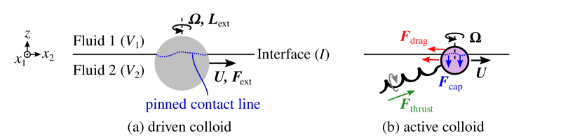
Figure 1: Driven and active colloids at interfaces. Panel (a) is a colloid adhered to a fluid interface by a pinned contact line driven into motion by external force and torque fields. In response to this forcing, the colloid translates parallel to the interface at velocity $\boldsymbol{U}$ and rotates on the axis normal to the interface at angular velocity $\boldsymbol{\Omega}$. Other motions are prohibited due to contact-line pinning and elevated surface tension. Panel (b) is a similar illustration of an active colloid; we take a motile bacterium as a natural example. Thrust generated by the rotating helical flagellum is balanced by drag due to viscous dissipation and capillary forces.

We consider a colloid adhered to a planar interface between two immiscible Newtonian fluids of viscosities $\mu_{1}$ and $\mu_{2}$, which are quiescent in the far field and together form an unbounded domain, as illustrated in figure 1. As described in section 1, we assume the resulting three-phase contact line is pinned, that is, it cannot move relative to the surface of the colloid. For simplicity, we further assume that the interface is flat. This assumption physically requires that (i) viscous stress due to flows generated by the particle are negligible compared to surface tension $\gamma$, which determines the equilibrium shape of the interface; (ii) the weight $mg$ of the colloid is also negligible compared to surface tension; and (iii) the amplitude of the undulations in the contact line are negligibly small compared to the size of the colloid. Requirement (i) is formally satisfied when $\mathinner{Ca}=\mu U/\gamma\ll 1$, where $\mathinner{Ca}$ is the capillary number, $\mu$ is the fluid viscosity and $U$ is the characteristic velocity of the colloid. For typical colloidal systems at air–aqueous or alkane–aqueous interfaces, $\mathinner{Ca}=O(${10}^{-7}$)$ to $O(${10}^{-5}$)$. Requirement (ii) is satisfied when $\mathinner{Bo}=mga^{2}/\gamma\ll 1$, where $\mathinner{Bo}$ is the particle Bond number and $a$ is the characteristic length scale of the colloid. In general, requirement (iii) may not be satisfied. For isolated passive particles, nanometric contact-line distortions alter the capillary energy that traps colloids on interfaces (Stamou et al., 2000), and thermally activated fluctuations at the contact line are hypothesized to alter dissipation in the interface (Boniello et al., 2015). Neither effect is included here, but the results we present may form the basis for a perturbative method to treat the problem of undulated contact lines.

At the colloidal scale, we may neglect the effects of fluid inertia and assume the flow on either side of the interface is governed by the Stokes equations,

$$\boldsymbol{\nabla}\boldsymbol{\cdot}\boldsymbol{\mathsfbi{\sigma}}=-\boldsymbol{\nabla}p+\mu\nabla^{2}\boldsymbol{u}=\boldsymbol{0};\quad\boldsymbol{\nabla}\boldsymbol{\cdot}\boldsymbol{u}=0,$$ (1)

where $\boldsymbol{\mathsfbi{\sigma}}$ is the stress tensor, $\boldsymbol{u}$ is the fluid velocity, $p$ is the hydrodynamic pressure and $\boldsymbol{\nabla}$ is the gradient operator. The stress tensor is given by $\boldsymbol{\mathsfbi{\sigma}}=-p\boldsymbol{\mathsfbi{I}}+\mu[\boldsymbol{\nabla}\boldsymbol{u}+{(\boldsymbol{\nabla}\boldsymbol{u})}^{\mathsf{T}}]$, where $\boldsymbol{\mathsfbi{I}}$ is the identity tensor. These quantities vary with the position vector $\boldsymbol{x}=x_{1}\hat{\boldsymbol{\imath}}_{1}+x_{2}\hat{\boldsymbol{\imath}}_{2}+z\hat{\boldsymbol{\imath}}_{3}$. Let $V_{1}$, $V_{2}$, and $I$ denote the set of points in fluid 1, fluid 2, and on the interface, respectively. We assume that the viscosity changes abruptly across the interface as $\mu(z)=\mu_{1}\operatorname{\mathbb{I}}_{\mathbb{R}_{+}}(z)+\mu_{2}\operatorname{\mathbb{I}}_{\mathbb{R}_{-}}(z)$, where the indicator function $\operatorname{\mathbb{I}}_{P}$ is unity if its argument is an element of $P$ but otherwise vanishes (e.g., $\operatorname{\mathbb{I}}_{\mathbb{R}_{+}}$ is equivalent to the Heaviside step function). On the interface, 1 satisfies the boundary conditions

$${\left[\boldsymbol{u}\right]}_{I} =\boldsymbol{0}$$ (2a)

$$\boldsymbol{n}\boldsymbol{\cdot}\boldsymbol{u}(\boldsymbol{x}\in I) =\boldsymbol{0}$$ (2b)

$$\boldsymbol{\nabla}_{\!\mathrm{s}}\boldsymbol{\cdot}\boldsymbol{\varsigma}+\boldsymbol{n}\boldsymbol{\cdot}{\left[\boldsymbol{\mathsfbi{\sigma}}\right]}_{I}\boldsymbol{\cdot}\boldsymbol{\mathsfbi{I}}_{\mathrm{s}} =\boldsymbol{0},$$ (2c)

where $\boldsymbol{n}$ is the unit normal to the interface pointing into fluid 1 and ${\left[f\right]}_{I}(\boldsymbol{x}\in I):=(\lim_{z\to 0^{+}}-\lim_{z\to 0^{-}})f(\boldsymbol{x})$ denotes the ‘jump’ in some function $f=f(\boldsymbol{x})$ across the interface going from fluid 2 to fluid 1. The first two conditions assert that the fluid velocity is continuous across $I$ 2a and that fluid does not pass through the interface 2b. The last condition 2c balances tangential stresses. Here, $\boldsymbol{\varsigma}=\boldsymbol{\varsigma}(\boldsymbol{x}\in I)$ is the surface stress tensor, $\boldsymbol{\mathsfbi{I}}_{\mathrm{s}}=\boldsymbol{\mathsfbi{I}}-\boldsymbol{nn}$ is the surface projection tensor, and $\boldsymbol{\nabla}_{\!\mathrm{s}}=\boldsymbol{\mathsfbi{I}}_{\mathrm{s}}\boldsymbol{\cdot}\boldsymbol{\nabla}$ is the surface gradient operator. Note that, since we assume that the interface is planar, $\boldsymbol{n}=\hat{\boldsymbol{\imath}}_{3}$ and $I$ is simply the set of points on $z=0$. Finally, as $|\boldsymbol{x}|\to\infty$, the fluid velocity and pressure gradient in either volume vanish, i.e., $\boldsymbol{u}(\boldsymbol{x})\to\boldsymbol{0}$ and $p(\boldsymbol{x})\to p_{\infty}$.

2.2 Clean interface

We call an interface ‘clean’ if it is free of surfactant molecules. In the absence of temperature gradients, a clean interface is characterized by a uniform surface tension $\gamma_{0}$, and $\boldsymbol{\varsigma}(\boldsymbol{x})=\gamma_{0}\boldsymbol{\mathsfbi{I}}_{\mathrm{s}}$. Then, $\boldsymbol{\nabla}_{\!\mathrm{s}}\boldsymbol{\cdot}\boldsymbol{\varsigma}$ vanishes and 2c reduces to

$$\boldsymbol{n}\boldsymbol{\cdot}{\left[\boldsymbol{\mathsfbi{\sigma}}\right]}_{I}\boldsymbol{\cdot}\boldsymbol{\mathsfbi{I}}_{\mathrm{s}}=\boldsymbol{0},$$ (3)

which states that the tangential stress on the fluid is continuous across the interface.

2.3 Incompressible interface

If surfactant is present, gradients in surfactant concentration due to flow exert Marangoni stresses on the surrounding fluids. At interfaces where $\mathinner{Ca}\ll 1$, these gradients need only be infinitesimal to balance viscous stresses due to colloid motion. As a result, the interface is constrained to surface-incompressible motion.

To derive the most conservative estimate for the effects of these Marangoni stresses, consider trace surfactant concentrations, for which the surfactant can be approximated as a two-dimensional ideal gas. We define the surface pressure as $\pi(\boldsymbol{x}\in I)=\gamma_{0}-\gamma(\boldsymbol{x}\in I)$. In this case, the dependence of the surface pressure on surfactant concentration $\Gamma=\Gamma(\boldsymbol{x}\in I)$ is given by $\partial\pi/\partial\Gamma=k_{B}T$, where $k_{B}$ is Boltzmann’s constant and $T$ is temperature. Scaling the surface pressure by viscous stresses $\tilde{\pi}=\pi/\bar{\mu}U$, where $\bar{\mu}=(\mu_{1}+\mu_{2})/2$ is the average surface viscosity, and letting $\tilde{\Gamma}=\Gamma/\bar{\Gamma}$, where $\bar{\Gamma}$ is the average surface concentration over the entire interface, we find that $\tilde{\boldsymbol{\nabla}_{\!\mathrm{s}}}\tilde{\pi}=\mathinner{Ma}\,\tilde{\boldsymbol{\nabla}_{\!\mathrm{s}}}\tilde{\Gamma}$, where the dimensionless parameter $\mathinner{Ma}={k_{B}T\bar{\Gamma}}/{\bar{\mu}U}$ is the Marangoni number and $\tilde{\boldsymbol{\nabla}_{\!\mathrm{s}}}=a\boldsymbol{\nabla}_{\!\mathrm{s}}$. To evaluate $\mathinner{Ma}$, we consider typical parameter values for a colloid moving at $U=$10\text{\,}\mathrm{\SIUnitSymbolMicro}\mathrm{m}\mathrm{/}\mathrm{s}$$ at a hexadecane-water interface ($\gamma_{0}\approx$50\text{\,}\mathrm{m}\mathrm{N}\mathrm{/}\mathrm{m}$$) in the surface-gaseous state. The surfactant concentration required to produce a $0.1\text{\,}\mathrm{\char 37\relax}$ decrease in the surface tension is approximately $\bar{\Gamma}=$2\text{\times}{10}^{3}\text{\,}\text{molecules}\mathrm{/}\mathrm{\SIUnitSymbolMicro}\mathrm{m}^{2}$$. Given $\bar{\mu}\approx$1\text{\,}\mathrm{mPa}\text{\,}\mathrm{s}$$, we estimate that $\mathinner{Ma}=O(10^{3})$. Thus, very small perturbations in $\Gamma$ generate sufficient Marangoni stress to balance viscous stresses due to motion of the colloid.

The large-$\mathinner{Ma}$ limit has the important consequence that the fluid interface behaves as incompressible layer ($\boldsymbol{\nabla}_{\!\mathrm{s}}\boldsymbol{\cdot}\boldsymbol{u}=0$). Assuming bulk-insoluble surfactant, the non-dimensionalized surfactant mass balance on the interface is

$$\tilde{\Gamma}(\boldsymbol{x})\,\tilde{\boldsymbol{\nabla}_{\!\mathrm{s}}}\boldsymbol{\cdot}\tilde{\boldsymbol{u}}+\mathinner{Ma}^{-1}(\tilde{\boldsymbol{u}}\boldsymbol{\cdot}\tilde{\boldsymbol{\nabla}_{\!\mathrm{s}}})\tilde{\pi}={(\mathinner{Ma}\,\mathinner{Pe}_{\mathrm{s}})}^{-1}\tilde{\nabla_{\!\mathrm{s}}^{2}}\tilde{\pi},$$ (4)

where $\tilde{\boldsymbol{u}}=\boldsymbol{u}/U$. Here, $\mathinner{Pe}_{\mathrm{s}}=Ua/D_{\mathrm{s}}$ represents the ‘interfacial’ Péclet number, where $D_{\mathrm{s}}$ is the surface diffusivity of the adsorbed surfactant. Equation 4 implies that $\tilde{\boldsymbol{\nabla}_{\!\mathrm{s}}}\boldsymbol{\cdot}\tilde{\boldsymbol{u}}\ll 1$ if $\mathinner{Ma}\gg 1$ and $\mathinner{Pe}_{\mathrm{s}}\gtrsim\mathinner{Ma}^{-1}$. Assuming $a=$10\text{\,}\mathrm{\SIUnitSymbolMicro m}$$ and $D_{\mathrm{s}}=${10}^{2}\text{\,}\mathrm{\SIUnitSymbolMicro}\mathrm{m}^{2}\mathrm{/}\mathrm{s}$$ (a typical value for small molecule surfactants), we have $\mathinner{Pe}_{\mathrm{s}}=O(1)$, so surfactant diffusion does not restore compressibility of the interface. At larger surfactant concentrations, the interface, populated by bulk-insoluble surfactants, generally departs from the surface-gaseous state. The interface generally remains incompressible in this case because, excluding phase transitions, $\partial\gamma/\partial\Gamma>k_{B}T$. Thus, we hereafter assume $\boldsymbol{\nabla}_{\!\mathrm{s}}\boldsymbol{\cdot}\boldsymbol{u}=0$ while discussing interfaces with surfactant. Dilute soluble surfactants also obey this constraint, as mass transport rates between the bulk and the interface are typically negligible. Note that we may express the Marangoni number as $\mathinner{Ma}=E/{\mathinner{Ca}}$, where $E=-(\bar{\Gamma}/\gamma)(\partial\gamma/\partial\Gamma)$ is the Gibbs elasticity. Thus, interfacial incompressibility is the typical circumstance for interfacial flow at low capillary number (Bławzdziewicz et al., 1999).

Surfactants can also create surface-viscous stresses due to shearing motion of the interface. If we assume Newtonian behavior, the interfacial stress tensor is given by

$$\boldsymbol{\varsigma}(\boldsymbol{x})=-\pi(\boldsymbol{x})\boldsymbol{\mathsfbi{I}}_{\mathrm{s}}+\mu_{\mathrm{s}}\left[\boldsymbol{\nabla}_{\!\mathrm{s}}\boldsymbol{u}+{(\boldsymbol{\nabla}_{\!\mathrm{s}}\boldsymbol{u})}^{\mathsf{T}}\right]$$ (5)

for $\boldsymbol{x}\in I$, where $\mu_{\mathrm{s}}$ is the surface viscosity. Then, 5 and 2c yield the tangential stress balance for an incompressible, surfactant-laden interface,

$$-\boldsymbol{\nabla}_{\!\mathrm{s}}\pi+\mu_{\mathrm{s}}\nabla_{\!\mathrm{s}}^{2}\boldsymbol{u}+\boldsymbol{n}\boldsymbol{\cdot}{\left[\boldsymbol{\mathsfbi{\sigma}}\right]}_{I}\boldsymbol{\cdot}\boldsymbol{\mathsfbi{I}}_{\mathrm{s}}=\boldsymbol{0}.$$ (6)

Equation 6 together with the incompressibility condition, $\boldsymbol{\nabla}_{\!\mathrm{s}}\boldsymbol{\cdot}\boldsymbol{u}=0$, are the Stokes equations for a two-dimensional Newtonian fluid being externally forced by bulk-viscous stresses.

3 Reciprocal relation for two fluids separated by an interface

3.1 Lorentz reciprocal theorem across an interface

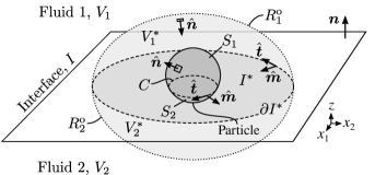
Figure 2: A colloidal particle, depicted in the center of the illustration, is surrounded by two arbitrary fluid regions $V^{*}_{1}\subset V_{1}$ and $V^{*}_{2}\subset V_{2}$, which meet at region $I^{*}\subset I$ on the interface. We assign the inward-facing normal vector $\hat{\boldsymbol{n}}$ to the boundaries of both of these regions. The unit normal to the interface $\boldsymbol{n}$ (sans hat) points in the $+z$ direction. The boundary of $V_{1}^{*}$ consists of the colloid surface $S_{1}$, the interfacial region $I^{*}$, and the remaining outer surface $R^{\text{o}}_{1}$, with the boundaries of $V_{2}^{*}$ being similarly labeled. The boundary of $I^{*}$ (dashed line), denoted $\partial I^{*}$, has the counterclockwise-oriented tangent vector $\hat{\boldsymbol{t}}$, and we define $\hat{\boldsymbol{m}}=\boldsymbol{n}\times\hat{\boldsymbol{t}}$, which points into $I^{*}$. The three-phase contact line $C$ comprises the inner part of $\partial I^{*}$.

The Lorentz reciprocal theorem provides a relation between the velocity and stress fields of two arbitrary Stokes flows. We may extend this theorem to two fluid regions separated by a clean or incompressible Newtonian interface as follows. Consider a region $V_{\nu}^{*}\subset V_{\nu}$ that is fully contained in fluid $\nu$, where $\nu=1\text{ or }2$, as illustrated by figure 2. Let $(\boldsymbol{u},\boldsymbol{\mathsfbi{\sigma}})$ and $(\boldsymbol{u}^{\prime},\boldsymbol{\mathsfbi{\sigma}}^{\prime})$ represent the velocity and stress fields of two different solutions to the inhomogeneous Stokes equations,

$$\boldsymbol{\nabla}\boldsymbol{\cdot}\boldsymbol{\mathsfbi{\sigma}}=-\boldsymbol{f}(\boldsymbol{x});\qquad\boldsymbol{\nabla}\boldsymbol{\cdot}\boldsymbol{\mathsfbi{\sigma}}^{\prime}=-\boldsymbol{f}^{\prime}(\boldsymbol{x}),$$ (7)

for $\boldsymbol{x}\in V^{*}_{\nu}$, each subject to the conditions given by 2 at the interface. Here, the forcing functions $\boldsymbol{f}$ and $\boldsymbol{f}^{\prime}$ aid in our generalization of the reciprocal theorem, as is customary in such derivations (Kim & Karrila, 1991). We will later assert that these quantities vanish. Integration of $\boldsymbol{\nabla}\boldsymbol{\cdot}(\boldsymbol{\mathsfbi{\sigma}}\boldsymbol{\cdot}\boldsymbol{u}^{\prime}-\boldsymbol{\mathsfbi{\sigma}}^{\prime}\boldsymbol{\cdot}\boldsymbol{u})$ over $V_{\nu}^{*}$ and application of the divergence theorem leads to the identity (see, e.g., Kim & Karrila, 1991)

$$\int_{V_{\nu}^{*}}[(\boldsymbol{\nabla}\boldsymbol{\cdot}\boldsymbol{\mathsfbi{\sigma}})\boldsymbol{\cdot}\boldsymbol{u}^{\prime}-(\boldsymbol{\nabla}\boldsymbol{\cdot}\boldsymbol{\mathsfbi{\sigma}}^{\prime})\boldsymbol{\cdot}\boldsymbol{u}]\mathop{}\!\mathrm{d}V+\int_{\partial V_{\nu}^{*}}(\boldsymbol{\mathsfbi{\sigma}}\boldsymbol{\cdot}\boldsymbol{u}^{\prime}-\boldsymbol{\mathsfbi{\sigma}}^{\prime}\boldsymbol{\cdot}\boldsymbol{u})\boldsymbol{\cdot}\mathop{}\!\mathrm{d}{\boldsymbol{S}}=0$$ (8)

where $\partial V_{\nu}^{*}$ denotes the boundary of $V_{\nu}^{*}$, and $\mathop{}\!\mathrm{d}{\boldsymbol{S}}=\hat{\boldsymbol{n}}\mathop{}\!\mathrm{d}S$ points into $V_{\nu}^{*}$. Substituting 7 into 8 gives the Lorentz reciprocal theorem,

$$\int_{V_{\nu}^{*}}[\boldsymbol{f}(\boldsymbol{x})\boldsymbol{\cdot}\boldsymbol{u}^{\prime}-\boldsymbol{f}^{\prime}(\boldsymbol{x})\boldsymbol{\cdot}\boldsymbol{u}]\mathop{}\!\mathrm{d}V=\int_{\partial V_{\nu}^{*}}(\boldsymbol{\mathsfbi{\sigma}}\boldsymbol{\cdot}\boldsymbol{u}^{\prime}-\boldsymbol{\mathsfbi{\sigma}}^{\prime}\boldsymbol{\cdot}\boldsymbol{u})\boldsymbol{\cdot}\mathop{}\!\mathrm{d}{\boldsymbol{S}}.$$ (9)

We add the pair of equations given by 9 for each of the two fluid phases ($\nu=1,2$) to obtain

$$\int_{V^{*}}[\boldsymbol{f}(\boldsymbol{x})\boldsymbol{\cdot}\boldsymbol{u}^{\prime}-\boldsymbol{f}^{\prime}(\boldsymbol{x})\boldsymbol{\cdot}\boldsymbol{u}]\mathop{}\!\mathrm{d}V\\ =\oint_{R}(\boldsymbol{\mathsfbi{\sigma}}\boldsymbol{\cdot}\boldsymbol{u}^{\prime}-\boldsymbol{\mathsfbi{\sigma}}^{\prime}\boldsymbol{\cdot}\boldsymbol{u})\boldsymbol{\cdot}\mathop{}\!\mathrm{d}{\boldsymbol{S}}+\int_{I^{*}}\left({\left[\boldsymbol{\mathsfbi{\sigma}}\right]}_{I}\boldsymbol{\cdot}\boldsymbol{u}^{\prime}-{\left[\boldsymbol{\mathsfbi{\sigma}}^{\prime}\right]}_{I}\boldsymbol{\cdot}\boldsymbol{u}\right)\boldsymbol{\cdot}\boldsymbol{n}\mathop{}\!\mathrm{d}A,$$ (10)

where $V^{*}:=V_{1}^{*}\cup V_{2}^{*}$ is the union of the fluid volumes in each phase, $I^{*}:=\partial V_{1}\cap\partial V_{2}$ is the region (at the fluid interface) where $V_{1}^{*}$ and $V_{2}^{*}$ ‘touch’, and $R:=\partial V^{*}\setminus I^{*}$ constitutes the remaining boundaries of $V_{1}^{*}$ and $V_{2}^{*}$ that are not adjacent to each other. For example, for the fluid region illustrated in figure 2, $R=S_{1}\cup S_{2}\cup R^{\text{o}}_{1}\cup R^{\text{o}}_{2}$, which includes both the surfaces of the colloid (the inner surfaces of $V^{*}$) and the outer surfaces of $V^{*}$. Note that $V^{*}_{1}$ and $V^{*}_{2}$ are disjoint subsets of $V^{*}$; they do not include points on $I$. We interpret the integral over $V^{*}$ in 10 as being a sum of integrations over each of these subsets, and we similarly interpret the integral over $R$. In the integral over $I^{*}$, we have used the fact that the fluid velocities $\boldsymbol{u}$ and $\boldsymbol{u}^{\prime}$ are continuous across the interface 2a. This term can be recast using the interfacial stress balance; contracting an arbitrary vector $\boldsymbol{t}^{*}$ directed tangent to the interface with 2c gives

$$(\boldsymbol{\nabla}_{\!\mathrm{s}}\boldsymbol{\cdot}\boldsymbol{\varsigma})\boldsymbol{\cdot}\boldsymbol{t}^{*}+\boldsymbol{n}\boldsymbol{\cdot}{\left[\boldsymbol{\mathsfbi{\sigma}}\right]}_{I}\boldsymbol{\cdot}\boldsymbol{t}^{*}+\boldsymbol{f}_{\mathrm{s}}\boldsymbol{\cdot}\boldsymbol{t}^{*}=0,$$ (11)

where we have included an additional external surface force density $\boldsymbol{f}_{\mathrm{s}}=\boldsymbol{f}_{\mathrm{s}}(\boldsymbol{x}\in I)$ on the interface. Since there is no fluid flux through interface, both $\boldsymbol{u}$ and $\boldsymbol{u}^{\prime}$ are tangent to the interface for $\boldsymbol{x}\in I$. Thus, 10 and 11 give, after replacing $\boldsymbol{t}^{*}$ with $\boldsymbol{u}$,

$$\int_{V^{*}}\left[\boldsymbol{f}\boldsymbol{\cdot}\boldsymbol{u}^{\prime}-\boldsymbol{f}^{\prime}\boldsymbol{\cdot}\boldsymbol{u}\right]\mathop{}\!\mathrm{d}{V}+\int_{I^{*}}\left[\boldsymbol{f}_{\mathrm{s}}\boldsymbol{\cdot}\boldsymbol{u}^{\prime}-\boldsymbol{f}_{\mathrm{s}}^{\prime}\boldsymbol{\cdot}\boldsymbol{u}\right]\mathop{}\!\mathrm{d}A\\ =\oint_{R}\left(\boldsymbol{\mathsfbi{\sigma}}\boldsymbol{\cdot}\boldsymbol{u}^{\prime}-\boldsymbol{\mathsfbi{\sigma}}^{\prime}\boldsymbol{\cdot}\boldsymbol{u}\right)\boldsymbol{\cdot}\mathop{}\!\mathrm{d}{\boldsymbol{S}}-\int_{I^{*}}\left[(\boldsymbol{\nabla}_{\!\mathrm{s}}\boldsymbol{\cdot}\boldsymbol{\varsigma})\boldsymbol{\cdot}\boldsymbol{u}^{\prime}-(\boldsymbol{\nabla}_{\!\mathrm{s}}\boldsymbol{\cdot}\boldsymbol{\varsigma}^{\prime})\boldsymbol{\cdot}\boldsymbol{u}\right]\mathop{}\!\mathrm{d}{A},$$ (12)

where $\boldsymbol{\varsigma}$ and $\boldsymbol{\varsigma}^{\prime}$ are the interfacial stress tensors associated with the unprimed and primed flows, respectively.

3.2 Clean interface

For a clean interface, $\boldsymbol{\varsigma}=-\boldsymbol{\mathsfbi{I}}_{\mathrm{s}}\gamma_{0}$ is constant, so the final integral in 12 vanishes;

$$\int_{V^{*}}\left[\boldsymbol{f}\boldsymbol{\cdot}\boldsymbol{u}^{\prime}-\boldsymbol{f}^{\prime}\boldsymbol{\cdot}\boldsymbol{u}\right]\mathop{}\!\mathrm{d}{V}+\int_{I^{*}}\left[\boldsymbol{f}_{\mathrm{s}}\boldsymbol{\cdot}\boldsymbol{u}^{\prime}-\boldsymbol{f}_{\mathrm{s}}^{\prime}\boldsymbol{\cdot}\boldsymbol{u}\right]\mathop{}\!\mathrm{d}{A}=\oint_{R}\left(\boldsymbol{\mathsfbi{\sigma}}\boldsymbol{\cdot}\boldsymbol{u}^{\prime}-\boldsymbol{\mathsfbi{\sigma}}^{\prime}\boldsymbol{\cdot}\boldsymbol{u}\right)\boldsymbol{\cdot}\mathop{}\!\mathrm{d}{\boldsymbol{S}}.$$ (13)

If we set $\boldsymbol{f}_{\mathrm{s}}=\boldsymbol{f}_{\mathrm{s}}^{\prime}=\boldsymbol{0}$, then the integral over $I^{*}$ in 13 also vanishes, which is the same as 9 with $\partial V_{\nu}^{*}$ replaced by $R$.

3.3 Incompressible interface

Assuming an incompressible interface with Newtonian behavior, as described by 5, there is a ‘surface’ reciprocal identity for the interface analogous to 9 given by

$$\int_{I^{*}}\left[(\boldsymbol{\nabla}_{\!\mathrm{s}}\boldsymbol{\cdot}\boldsymbol{\varsigma})\boldsymbol{\cdot}\boldsymbol{u}^{\prime}-(\boldsymbol{\nabla}_{\!\mathrm{s}}\boldsymbol{\cdot}\boldsymbol{\varsigma}^{\prime})\boldsymbol{\cdot}\boldsymbol{u}\right]\mathop{}\!\mathrm{d}A+\oint_{\partial I^{*}}{(\boldsymbol{\varsigma}\boldsymbol{\cdot}\boldsymbol{u}^{\prime}-\boldsymbol{\varsigma}^{\prime}\boldsymbol{\cdot}\boldsymbol{u})}\boldsymbol{\cdot}\hat{\boldsymbol{m}}\mathop{}\!\mathrm{d}C=0,$$ (14)

where the contour integral is taken over the boundary of $I^{*}$, denoted $\partial I^{*}$. For the system of a particle on an interface illustrated in figure 2, $\partial I^{*}$ includes the contact line on the particle $C$ as its inner boundary. We assign $\partial I^{*}$ the unit tangent vector $\hat{\boldsymbol{t}}$ regarding $I^{*}$ as a counterclockwise-oriented surface. The unit vector $\hat{\boldsymbol{m}}=\boldsymbol{n}\times\hat{\boldsymbol{t}}$ points into the interfacial region $I^{*}$, meeting $\partial I^{*}$ at a right angle. Equations 14 and 12 yield

$$\int_{V^{*}}\left[\boldsymbol{f}\boldsymbol{\cdot}\boldsymbol{u}^{\prime}-\boldsymbol{f}^{\prime}\boldsymbol{\cdot}\boldsymbol{u}\right]\mathop{}\!\mathrm{d}{V}+\int_{I^{*}}\left[\boldsymbol{f}_{\mathrm{s}}\boldsymbol{\cdot}\boldsymbol{u}^{\prime}-\boldsymbol{f}_{\mathrm{s}}^{\prime}\boldsymbol{\cdot}\boldsymbol{u}\right]\mathop{}\!\mathrm{d}A\\ =\oint_{R}\left(\boldsymbol{\mathsfbi{\sigma}}\boldsymbol{\cdot}\boldsymbol{u}^{\prime}-\boldsymbol{\mathsfbi{\sigma}}^{\prime}\boldsymbol{\cdot}\boldsymbol{u}\right)\boldsymbol{\cdot}\mathop{}\!\mathrm{d}{\boldsymbol{S}}+\oint_{\partial I^{*}}\left(\boldsymbol{\varsigma}\boldsymbol{\cdot}\boldsymbol{u}^{\prime}-\boldsymbol{\varsigma}^{\prime}\boldsymbol{\cdot}\boldsymbol{u}\right)\boldsymbol{\cdot}\hat{\boldsymbol{m}}\mathop{}\!\mathrm{d}C.$$ (15)

Comparing 15 to the analogous equation for a clean interface 13, we see that the final integral on the right-hand side is new. This contour integral over the boundary of $I^{*}$ accounts for surface pressure gradients, or Marangoni stresses, that enforce the interfacial incompressibility constraint and, if $\mu_{\mathrm{s}}>0$, for surface-viscous dissipation. While we restrict ourselves to planar interfaces, 13 and 15 hold even if the interface is curved, given that it has the same shape in both the primed and unprimed flow problems.

4 Clean fluid interfaces

While incompressible interfaces are typical for colloidal systems, as described in section 2.3, it is instructive to first consider clean interfaces. In this section, we develop the multipole expansion for a colloid at a clean interface. In section 4.1, we review the Green’s function for a clean interface, originally developed by Aderogba & Blake (1978). Then, in section 4.2, we use 13 to derive a boundary integral representation of the velocity field appropriate for developing the multipole expansion, which is done in section 4.3. Finally, we discuss the implications of the leading-order multipoles for driven and active colloids on interfaces.

4.1 Green’s function

Due to the linearity of the Stokes equations 1 and its boundary conditions for a clean interface 3, we may represent the velocity field due to a point force located at $\boldsymbol{y}=y_{1}\hat{\boldsymbol{\imath}}_{1}+y_{2}\hat{\boldsymbol{\imath}}_{2}+h\hat{\boldsymbol{\imath}}_{3}$ as $\boldsymbol{u}(\boldsymbol{x})=\boldsymbol{\mathsfbi{G}}(\boldsymbol{x},\boldsymbol{y})\boldsymbol{\cdot}\boldsymbol{F}$, where $\boldsymbol{\mathsfbi{G}}$ is the Green’s function for two fluids separated by a clean interface. This Green’s function satisfies the (inhomogeneous) Stokes equations

$$-\boldsymbol{\nabla}\boldsymbol{P}(\boldsymbol{\mathsfbi{G}};\boldsymbol{x},\boldsymbol{y})+\mu(z)\,\nabla^{2}\boldsymbol{\mathsfbi{G}}(\boldsymbol{x},\boldsymbol{y}) =\begin{cases}\boldsymbol{0}&h=0\\ -\boldsymbol{\mathsfbi{I}}\delta_{\mathbb{R}^{3}}(\boldsymbol{x}-\boldsymbol{y})&h\neq 0\end{cases}$$ (16a)

$$\boldsymbol{\nabla}\boldsymbol{\cdot}\boldsymbol{\mathsfbi{G}}(\boldsymbol{x},\boldsymbol{y}) =\boldsymbol{0}$$ (16b)

for $\boldsymbol{x}\in V_{1}\cup V_{2}$. Equation 16 is subject to the far-field condition $\boldsymbol{\mathsfbi{G}}\to\boldsymbol{0}$ as $|\boldsymbol{x}|\to\infty$, the interfacial stress balance

$$\boldsymbol{\mathsfbi{I}}_{\mathrm{s}}\boldsymbol{\cdot}{\left[\boldsymbol{n}\boldsymbol{\cdot}\boldsymbol{\mathsfbi{T}}(\boldsymbol{\mathsfbi{G}};\boldsymbol{x},\boldsymbol{y})\right]}_{I} =\begin{cases}-\boldsymbol{\mathsfbi{I}}_{\mathrm{s}}\delta_{\mathbb{R}^{2}}(\boldsymbol{x}-\boldsymbol{y})&h=0\\ \boldsymbol{0}&h\neq 0,\end{cases}$$ (17a)

and the kinematic conditions

$$\boldsymbol{t}^{*}\boldsymbol{\cdot}{\left[\boldsymbol{\mathsfbi{G}}(\boldsymbol{x},\boldsymbol{y})\right]}_{I} =\boldsymbol{n}\boldsymbol{\cdot}\boldsymbol{\mathsfbi{G}}(\boldsymbol{x}\in I)=\boldsymbol{0}.$$ (17b)

Here, $\boldsymbol{P}(\boldsymbol{\mathsfbi{G}};\!)$ is the (vectorial) pressure field associated with $\boldsymbol{\mathsfbi{G}}$, $\boldsymbol{\mathsfbi{T}}(\boldsymbol{\mathsfbi{G}};\!)$ is the stress tensor associated with $\boldsymbol{\mathsfbi{G}}$, and $\delta_{\mathbb{R}^{n}}(\boldsymbol{x})$ is the Dirac delta in $\mathbb{R}^{n}$. As expressed by 17a, for $h=0$, we consider the point force to be exerted on the interface itself rather than on one of the fluids. Equations 16 and 17 follow directly from 1 and 2 after factoring out $\boldsymbol{F}$ from both sides of each of these equations.

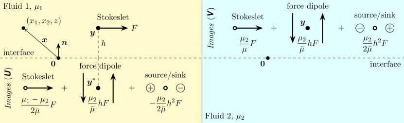
Figure 3: A point force of magnitude $F=|\boldsymbol{F}|$ parallel to the interface induces the image system illustrated above, as expressed by 18. The upper left and lower right portions of the figure represent the physical fluid phases while the upper right and lower left are fictitious image domains that contain singularities acting to satisfy the boundary conditions on the interface 17. The image singularities in each image domain are depicted separately for clarity, but they all act at the same image point, i.e., $\boldsymbol{y}^{*}$ for fluid 1 and $\boldsymbol{y}$ for fluid 2.

Solving 16 and 17 yields

$$\boldsymbol{\mathsfbi{G}}(\boldsymbol{x},\boldsymbol{y})=\begin{cases}[\boldsymbol{\mathsfbi{J}}(\boldsymbol{x}-\boldsymbol{y})+\boldsymbol{\mathsfbi{U}}(\boldsymbol{x},\boldsymbol{y}^{*})]/\mu(h)&zh\geq 0\\ \boldsymbol{\mathsfbi{V}}(\boldsymbol{x},\boldsymbol{y})/\bar{\mu}&zh\leq 0\\ \boldsymbol{\mathsfbi{J}}(\boldsymbol{x}-\boldsymbol{y})\boldsymbol{\cdot}\boldsymbol{\mathsfbi{I}}_{\mathrm{s}}/\bar{\mu}&h=0,\end{cases}$$ (18)

where $\boldsymbol{y}^{*}=(y_{1},y_{2},-h)$ is the reflection of $\boldsymbol{y}$ through $z=0$. Equation 18 expresses $\boldsymbol{\mathsfbi{G}}$ as a functional of the Oseen tensor $\boldsymbol{\mathsfbi{J}}(\boldsymbol{x})=(\boldsymbol{\mathsfbi{I}}/|\boldsymbol{x}|-\boldsymbol{x}\boldsymbol{x}/|\boldsymbol{x}|^{3})/8\upi$. The tensors $\boldsymbol{\mathsfbi{U}}$ and $\boldsymbol{\mathsfbi{V}}$ represent the hydrodynamic images necessary to satisfy continuity of tangential stress 17a and continuity of velocity at the interface. These image systems are given by (Aderogba & Blake, 1978)

$$\mathsfi U_{ij}(\boldsymbol{x},\boldsymbol{\xi}) =(\delta^{\shortparallel}_{jk}-n_{j}n_{k})\mathsfi J_{ik}(\boldsymbol{x}-\boldsymbol{\xi})-\frac{\mu(\boldsymbol{\xi}\boldsymbol{\cdot}\boldsymbol{n})}{\bar{\mu}}\mathsfi V_{ik}(\boldsymbol{x},\boldsymbol{\xi})$$ (19)

$$\mathsfi V_{ij}(\boldsymbol{x},\boldsymbol{\xi}) =\left\{\delta^{\shortparallel}_{jk}+(\delta^{\shortparallel}_{jk}-n_{j}n_{k})\left[(\boldsymbol{\xi}\boldsymbol{\cdot}\boldsymbol{n})n_{l}\frac{\partial}{\partial\xi_{k}}-\frac{1}{2}(\boldsymbol{\xi}\boldsymbol{\cdot}\boldsymbol{n})^{2}\delta_{kl}\nabla^{2}\right]\right\}\mathsfi J_{il}(\boldsymbol{x}-\boldsymbol{\xi}),$$ (20)

where $\delta_{jk}$ is the Kronecker delta and $\delta^{\shortparallel}_{jk}=\delta_{jk}-n_{j}n_{k}$. The tensor indices $i,j,k,l\in\{1,2,3\}$ follow the Einstein summation convention.

Equation 18 partitions $\boldsymbol{\mathsfbi{G}}(\boldsymbol{x},\boldsymbol{y})$ into three cases: $zh\geq 0$, where $\boldsymbol{x}$ and $\boldsymbol{y}$ are in the same fluid; $zh\leq 0$, where $\boldsymbol{x}$ and $\boldsymbol{y}$ are in different fluids; and $h=0$ for all $z$, where $\boldsymbol{y}\in I$. Without loss of generality, if we let the point force at $\boldsymbol{y}$ be in the upper fluid ($h>0$), then a Stokeslet, the fundamental solution to the Stokes equations in an unbounded fluid given by $\boldsymbol{\mathsfbi{J}}/8\upi\mu_{1}$, is induced at this point. Examining, 20, the flow in the lower fluid ($z<0$) comprises three image flows: a Stokeslet parallel to the interface, a Stokeslet dipole, and a degenerate Stokes quadrupole (a source–sink doublet), all of which have their singular points at $\boldsymbol{y}$. These images are depicted on the upper right-hand (cyan) side of figure 3. The image system $\boldsymbol{\mathsfbi{U}}$ for the upper fluid 19 is similar except that the image singularities are located at the image point $\boldsymbol{y}^{*}$, depicted on the lower left-hand (yellow) side of figure 3. This image system additionally includes a copy of the original forcing Stokeslet reflected through $z=0$.

Finally, we note two properties of $\boldsymbol{\mathsfbi{G}}$ that will be useful in the analysis that follows. First, it is self-adjoint,

$$\boldsymbol{\mathsfbi{G}}(\boldsymbol{x},\boldsymbol{y})=\boldsymbol{\mathsfbi{G}}^{\mathsf{T}}(\boldsymbol{y},\boldsymbol{x}),$$ (21)

which may be proven using 13 (see appendix A) or directly verified from 18. The second property concerns the limiting behavior of $\boldsymbol{\mathsfbi{G}}$. As $|\boldsymbol{x}|$ becomes large for fixed $|\boldsymbol{y}|$, $\boldsymbol{\mathsfbi{G}}(\boldsymbol{x},\boldsymbol{y})\boldsymbol{\cdot}\boldsymbol{F}$ effectively appears as a Stokeslet and decays as ${|\boldsymbol{x}-\boldsymbol{y}|}^{-1}\sim{|\boldsymbol{x}|}^{-1}$; the image Stokes dipole and degenerate quadrupole terms, contained in $\boldsymbol{\mathsfbi{U}}$ and $\boldsymbol{\mathsfbi{V}}$, do not affect the far-field behavior of $\boldsymbol{\mathsfbi{G}}$ because their spatial decay is more rapid than that of the Stokeslet. An exception occurs when $\boldsymbol{F}$ points directly away from the interface, in which case $\boldsymbol{\mathsfbi{G}}\boldsymbol{\cdot}\boldsymbol{F}$ reduces to an effective stresslet of strength $h|\boldsymbol{F}|\mu(h)/\bar{\mu}$ for $|\boldsymbol{x}|\gg|\boldsymbol{y}|$ and decays as ${|\boldsymbol{x}|}^{-2}$ (Aderogba & Blake, 1978). By 21, the decay behavior of $\boldsymbol{\mathsfbi{G}}$ for fixed $\boldsymbol{x}$ as $\boldsymbol{y}$ is made large reflects the behavior for fixed $\boldsymbol{y}$ as $\boldsymbol{x}$ is made large; $\boldsymbol{\mathsfbi{G}}(\boldsymbol{x},\boldsymbol{y})\sim{|\boldsymbol{y}|}^{-1}$ for $\boldsymbol{y}\gg\boldsymbol{x}$.

4.2 Boundary integral equation

Using the Green’s function 18 as the ‘primed’ flow field in the reciprocal relation 13, we may generate a boundary integral equation for an object at the interface. Consider the interfacially trapped colloid, illustrated in figure 2, whose upper surface $S_{1}$ is in contact with fluid 1 and whose lower surface $S_{2}$ is in contact with fluid 2. An arbitrary volume of fluid $V^{*}=V^{*}_{1}\cup V^{*}_{2}$ surrounds the colloid, which is bounded by $S_{1}$ and $S_{2}$ as well as the outer fluid surfaces $R^{\text{o}}_{1}$ and $R^{\text{o}}_{2}$. We make the following substitutions into 13: $\boldsymbol{u}^{\prime}(\boldsymbol{x})\to\boldsymbol{\mathsfbi{G}}(\boldsymbol{x},\boldsymbol{y})$, $\boldsymbol{\mathsfbi{\sigma}}^{\prime}(\boldsymbol{x})\to\boldsymbol{\mathsfbi{T}}(\boldsymbol{\mathsfbi{G}};\boldsymbol{x},\boldsymbol{y})$, $\boldsymbol{f}^{\prime}\to\boldsymbol{\mathsfbi{I}}\delta_{\mathbb{R}^{3}}(\boldsymbol{x}-\boldsymbol{y})$, and $\boldsymbol{f}_{\mathrm{s}}^{\prime}\to\boldsymbol{\mathsfbi{I}}\delta_{\mathbb{R}^{2}}(\boldsymbol{x}-\boldsymbol{y})$ to find

$$\int_{V*}\mathopen{\big{[}}\boldsymbol{f}\boldsymbol{\cdot}\boldsymbol{\mathsfbi{G}}(\boldsymbol{x},\boldsymbol{y})-\boldsymbol{\mathsfbi{I}}\delta_{\mathbb{R}^{3}}(\boldsymbol{x}-\boldsymbol{y})\boldsymbol{\cdot}\boldsymbol{u}(\boldsymbol{x})\mathclose{\big{]}}\mathop{}\!\mathrm{d}{V(\boldsymbol{x})}+\int_{I^{*}}\mathopen{\big{[}}\boldsymbol{f}_{\mathrm{s}}\boldsymbol{\cdot}\boldsymbol{\mathsfbi{G}}(\boldsymbol{x},\boldsymbol{y})-\boldsymbol{\mathsfbi{I}}_{\mathrm{s}}\delta_{\mathbb{R}^{2}}(\boldsymbol{x}-\boldsymbol{y})\boldsymbol{\cdot}\boldsymbol{u}\mathclose{\big{]}}\mathop{}\!\mathrm{d}{A(\boldsymbol{x})}\\ =\oint_{R}\bigl{\{}\hat{\boldsymbol{n}}(\boldsymbol{x})\boldsymbol{\cdot}\boldsymbol{\mathsfbi{\sigma}}(\boldsymbol{x})\boldsymbol{\cdot}\boldsymbol{\mathsfbi{G}}(\boldsymbol{x},\boldsymbol{y})-\boldsymbol{u}(\boldsymbol{x})\boldsymbol{\cdot}\bigl{[}\hat{\boldsymbol{n}}(\boldsymbol{x})\boldsymbol{\cdot}\boldsymbol{\mathsfbi{T}}(\boldsymbol{\mathsfbi{G}};\boldsymbol{x},\boldsymbol{y})\bigr{]}\bigr{\}}\mathop{}\!\mathrm{d}{S(\boldsymbol{x})}.$$ (22)

We assert that the external force densities $\boldsymbol{f}$ and $\boldsymbol{f}_{\mathrm{s}}$ vanish in 22. Using the identity $\int_{\Omega}\delta_{\mathbb{R}^{n}}(\boldsymbol{x}-\boldsymbol{y})\,f(\boldsymbol{x})\mathop{}\!\mathrm{d}^{n}{\boldsymbol{x}}=\operatorname{\mathbb{I}}_{\Omega}(\boldsymbol{y})\,f(\boldsymbol{y})$, where $f$ and $\Omega$ are arbitrary, 22 becomes

$$\operatorname{\mathbb{I}}_{V^{*}}(\boldsymbol{y})\,\boldsymbol{u}(\boldsymbol{y})+\operatorname{\mathbb{I}}_{I^{*}}(\boldsymbol{y})\,\boldsymbol{\mathsfbi{I}}_{\mathrm{s}}\boldsymbol{\cdot}\boldsymbol{u}(\boldsymbol{y})$$ (23)

$$\quad=\oint_{R}\bigl{\{}\hat{\boldsymbol{n}}(\boldsymbol{x})\boldsymbol{\cdot}\boldsymbol{\mathsfbi{\sigma}}(\boldsymbol{x})\boldsymbol{\cdot}\boldsymbol{\mathsfbi{G}}(\boldsymbol{x},\boldsymbol{y})-\boldsymbol{u}(\boldsymbol{x})\boldsymbol{\cdot}\bigl{[}\hat{\boldsymbol{n}}(\boldsymbol{x})\boldsymbol{\cdot}\boldsymbol{\mathsfbi{T}}(\boldsymbol{\mathsfbi{G}};\boldsymbol{x},\boldsymbol{y})\bigr{]}\bigr{\}}\mathop{}\!\mathrm{d}{S(\boldsymbol{x})}.$$

The first term on the left-hand side of 23 gives the velocity field (as a function of $\boldsymbol{y}$) whenever $\boldsymbol{y}\in V^{*}$ (i.e., $\boldsymbol{y}$ is in either $V^{*}_{1}$ or $V^{*}_{2}$, not including points on the interface) and elsewhere vanishes. The following term is complementary and vanishes unless $\boldsymbol{y}$ lies right on $I^{*}$; the surface projection $\boldsymbol{\mathsfbi{I}}_{\mathrm{s}}$ has no effect here due to the no-penetration condition 2b.

In the limit that $V^{*}\to V$ and $I^{*}\to I$, such that the shaded regions in figure 2 grow to fill the entire domain, with $R^{\text{o}}_{1}$ and $R^{\text{o}}_{2}$ becoming arbitrarily far away from the colloid, we find that 23 gives the boundary integral representation for the velocity field,

$$\boldsymbol{u}(\boldsymbol{x})=-\oint_{S_{\text{c}}}\boldsymbol{\mathsfbi{G}}(\boldsymbol{x},\boldsymbol{y})\boldsymbol{\cdot}[\boldsymbol{\mathsfbi{\sigma}}\boldsymbol{\cdot}\hat{\boldsymbol{n}}](\boldsymbol{y})\mathop{}\!\mathrm{d}S(\boldsymbol{y})+\oint_{S_{\text{c}}}{[\boldsymbol{u}\hat{\boldsymbol{n}}]}(\boldsymbol{y})\odot\boldsymbol{\mathsfbi{T}}(\boldsymbol{\mathsfbi{G}};\boldsymbol{y},\boldsymbol{x})\mathop{}\!\mathrm{d}S(\boldsymbol{y}),$$ (24)

where $S_{\text{c}}=S_{1}\cup S_{2}$ represents the surface of the colloid and the operator ‘$\odot$’ denotes complete contraction of its operands, e.g., $(\boldsymbol{\mathsfbi{A}}\odot\boldsymbol{\mathsfbi{B}})_{j_{1}\dots j_{m}}=\mathsfi A_{i_{1}\dots i_{n}}\mathsfi B_{i_{n}\dots i_{1}j_{1}\dots j_{m}}$ if $\boldsymbol{\mathsfbi{A}}$ is the tensor of lower rank and $(\boldsymbol{\mathsfbi{A}}\odot\boldsymbol{\mathsfbi{B}})_{j_{1}\cdots j_{m}}=\mathsfi A_{j_{1}\cdots j_{m}i_{1}\cdots i_{n}}\mathsfi B_{i_{n}\cdots i_{1}}$ if $\boldsymbol{\mathsfbi{B}}$ is the tensor of lower rank. We have exchanged $\boldsymbol{y}$ and $\boldsymbol{x}$ going from 23 to 24 to make $\boldsymbol{x}$ be the observation point of $\boldsymbol{u}(\boldsymbol{x})$ and $\boldsymbol{y}$ be the integration variable. We have also used the self-adjoint property of $\boldsymbol{\mathsfbi{G}}$ 21 in the first term on the right-hand side of 24. The convergence of 23 to 24 follows from the decay behavior of $\boldsymbol{\mathsfbi{G}}(\boldsymbol{x},\boldsymbol{y})$ and from the quiescent state of the fluid far from the colloid. Equation 24 is valid as long as the colloid does not deform in a manner that would distort the flat shape of the pinned contact line.

Equation 24 is similar in form and interpretation to the boundary integral equation for Stokes flows that appears in standard textbooks (see, e.g., Kim & Karrila, 1991; Pozrikidis, 1992). Indeed, 24 is derived in an analogous manner using the generalized reciprocal relation 13. The key property of 24 is that, by construction, integrals over the interface itself do not appear because $\boldsymbol{\mathsfbi{G}}$ and $\boldsymbol{\mathsfbi{T}}$ implicitly account for transmission of hydrodynamic stresses through the interface. This property allows for straightforward generation of the multipole expansion in the following section.

4.3 Multipole expansion

To generate a multipole expansion for $\boldsymbol{u}(\boldsymbol{x})$, we replace $\boldsymbol{\mathsfbi{G}}(\boldsymbol{x},\boldsymbol{y})$ and $\boldsymbol{\mathsfbi{T}}(\boldsymbol{\mathsfbi{G}};\boldsymbol{x},\boldsymbol{y})$ in 24 with their Taylor series in $\boldsymbol{y}$ about an point on the interface as near as possible to the center of the colloid, which we designate as the origin $\boldsymbol{0}$. This process is slightly complicated by the piecewise nature of $\boldsymbol{\mathsfbi{G}}$ as $\boldsymbol{y}$ passes from one side of the interface to the other. In particular, certain components of $\boldsymbol{\nabla}_{\boldsymbol{y}}\boldsymbol{\mathsfbi{G}}(\boldsymbol{x},\boldsymbol{y})$ contain a jump discontinuity over the interface at $z=0$. This difficulty is overcome by separating each integral in 24 into one over $S_{1}$ and another over $S_{2}$, so that the integrand is continuous over each of these surfaces. Letting $\boldsymbol{u}^{(1)}$ and $\boldsymbol{u}^{(2)}$ denote the contributions from integration over $S_{1}$ and $S_{2}$, respectively, we may write the expansion as $\boldsymbol{u}=\boldsymbol{u}^{(1)}+\boldsymbol{u}^{(2)}$, where

$$\boldsymbol{u}^{(1)}(\boldsymbol{x})=-\sum_{n=0}^{\infty}\frac{1}{n!}\left(\int_{S_{1}}[\hat{\boldsymbol{n}}\boldsymbol{\cdot}\boldsymbol{\mathsfbi{\sigma}}](\boldsymbol{y})\,\boldsymbol{y}^{\boldsymbol{\otimes}n}\mathop{}\!\mathrm{d}S(\boldsymbol{y})\right) \odot\left(\lim_{\boldsymbol{y}\to\boldsymbol{0}^{+}}\boldsymbol{\nabla}_{\boldsymbol{y}}^{\boldsymbol{\otimes}n}\boldsymbol{\mathsfbi{G}}^{\mathsf{T}}(\boldsymbol{x},\boldsymbol{y})\right)$$ (25)

$$+\sum_{n=0}^{\infty}\frac{1}{n!}\left(\int_{S_{1}}[\boldsymbol{u}\hat{\boldsymbol{n}}](\boldsymbol{y})\,\boldsymbol{y}^{\boldsymbol{\otimes}n}\mathop{}\!\mathrm{d}S(\boldsymbol{y})\right) \odot\left(\lim_{\boldsymbol{y}\to\boldsymbol{0}^{+}}\boldsymbol{\nabla}_{\boldsymbol{y}}^{\boldsymbol{\otimes}n}\boldsymbol{\mathsfbi{T}}(\boldsymbol{\mathsfbi{G}};\boldsymbol{y},\boldsymbol{x})\right)$$

and

$$\boldsymbol{u}^{(2)}(\boldsymbol{x})=-\sum_{n=0}^{\infty}\frac{1}{n!}\left(\int_{S_{2}}[\hat{\boldsymbol{n}}\boldsymbol{\cdot}\boldsymbol{\mathsfbi{\sigma}}](\boldsymbol{y})\,\boldsymbol{y}^{\boldsymbol{\otimes}n}\mathop{}\!\mathrm{d}S(\boldsymbol{y})\right) \odot\left(\lim_{\boldsymbol{y}\to\boldsymbol{0}^{-}}\boldsymbol{\nabla}_{\boldsymbol{y}}^{\boldsymbol{\otimes}n}\boldsymbol{\mathsfbi{G}}^{\mathsf{T}}(\boldsymbol{x},\boldsymbol{y})\right)$$ (26)

$$+\sum_{n=0}^{\infty}\frac{1}{n!}\left(\int_{S_{2}}[\boldsymbol{u}\hat{\boldsymbol{n}}](\boldsymbol{y})\,\boldsymbol{y}^{\boldsymbol{\otimes}n}\mathop{}\!\mathrm{d}S(\boldsymbol{y})\right) \odot\left(\lim_{\boldsymbol{y}\to\boldsymbol{0}^{-}}\boldsymbol{\nabla}_{\boldsymbol{y}}^{\boldsymbol{\otimes}n}\boldsymbol{\mathsfbi{T}}(\boldsymbol{\mathsfbi{G}};\boldsymbol{y},\boldsymbol{x})\right)$$

Here, $\boldsymbol{y}^{\boldsymbol{\otimes}n}=\boldsymbol{y}\boldsymbol{y}\cdots$ ($n$ times) denotes the $n$-fold tensor product and $\boldsymbol{\nabla}_{\boldsymbol{y}}^{\boldsymbol{\otimes}n}$ similarly denotes the $n$-fold gradient operator. Writing $\boldsymbol{\mathsfbi{T}}$ in terms of $\boldsymbol{\mathsfbi{G}}$ as

$$\mathsfi T_{ijk}(\boldsymbol{\mathsfbi{G}};\boldsymbol{y},\boldsymbol{x})=-\delta_{ij}P_{k}(\boldsymbol{\mathsfbi{G}};\boldsymbol{y},\boldsymbol{x})+\mu(h)\left(\frac{\partial\mathsfi G_{kj}(\boldsymbol{x},\boldsymbol{y})}{\partial y_{i}}+\frac{\partial\mathsfi G_{ki}(\boldsymbol{x},\boldsymbol{y})}{\partial y_{j}}\right)$$

and collecting terms in $\boldsymbol{\mathsfbi{G}}$, ${\boldsymbol{\nabla}}_{\!\boldsymbol{y}}\boldsymbol{\mathsfbi{G}}$, and so on for higher-order gradients of $\boldsymbol{\mathsfbi{G}}$, we arrive at the multipole expansion,

$$\boldsymbol{u}(\boldsymbol{x})=\boldsymbol{u}^{\text{m0}}(\boldsymbol{x})+\boldsymbol{u}^{\text{m1}}(\boldsymbol{x})+\boldsymbol{u}^{\text{m2}}(\boldsymbol{x})+\text{h.o.t},$$ (27)

where $$\boldsymbol{u}^{\text{m0}} \boldsymbol{u}^{\text{m1}} \boldsymbol{u}^{\text{m2}}$$ is the force-monopole (zeroth) moment, is the force-dipole (first) moment, is the quadrupole (second) moment, and so on for higher-order terms (h.o.t.). In particular, these first three moments are given by

$$u^{\text{m0}}_{i}(\boldsymbol{x}) =F^{(1)}_{i}\mathsfi G_{ij}(\boldsymbol{x},\boldsymbol{0}^{+})+F^{(2)}_{i}\mathsfi G_{ij}(\boldsymbol{x},\boldsymbol{0}^{-})$$ (27a)

$$u^{\text{m1}}_{i}(\boldsymbol{x}) =\mathsfi D^{(1)}_{jk}\frac{\partial\mathsfi G_{ij}}{\partial y_{k}}(\boldsymbol{x},\boldsymbol{0}^{+})+\mathsfi D^{(2)}_{jk}\frac{\partial\mathsfi G_{ij}}{\partial y_{k}}(\boldsymbol{x},\boldsymbol{0}^{-})$$ (27b)

$$u^{\text{m2}}_{i}(\boldsymbol{x}) =\mathsfi Q^{(1)}_{jkl}\frac{\partial^{2}\mathsfi G_{ij}}{\partial y_{l}\partial y_{k}}(\boldsymbol{x},\boldsymbol{0}^{+})+\mathsfi Q^{(2)}_{jkl}\frac{\partial^{2}\mathsfi G_{ij}}{\partial y_{l}\partial y_{k}}(\boldsymbol{x},\boldsymbol{0}^{-}),$$ (27c)

where $\boldsymbol{F}^{(\nu)}$, $\boldsymbol{\mathsfbi{D}}^{(\nu)}$, and $\boldsymbol{\mathsfbi{Q}}^{(\nu)}$ are the monopole, dipole, and quadrupole coefficients for fluid $\nu\in\{1,2\}$, respectively. The shorthand notation $\boldsymbol{0}^{+}$ indicates the limit as $\boldsymbol{y}$ approaches $\boldsymbol{0}$ from above the interface (i.e., from fluid 1). Similarly, $\boldsymbol{0}^{-}$ indicates the limit as $\boldsymbol{y}$ approaches $\boldsymbol{0}$ from below. In 27b, we have assumed, for simplicity, that the colloid does not grow or shrink in volume so that there is no source or sink flow from the origin. Note that if the colloid is wholly immersed in one fluid, then the multipole coefficients for the other fluid vanish.

At distances far enough from the colloid that points on the colloid surface are virtually indistinguishable from $\boldsymbol{0}$, $|\boldsymbol{x}|\gg a$, the leading terms of 27 closely approximate $\boldsymbol{u}(\boldsymbol{x})$. Recall that $\boldsymbol{\mathsfbi{G}}(\boldsymbol{x},\boldsymbol{y})\sim{|\boldsymbol{x}|}^{-1}$ for $|\boldsymbol{x}|\gg|\boldsymbol{y}|$. It follows that $\boldsymbol{u}^{\text{m0}}(\boldsymbol{x})\sim r^{-1}$, where $r=|\boldsymbol{x}|$. Each successive multipole moment involves a higher-order gradient of $\boldsymbol{\mathsfbi{G}}$. Thus, $\boldsymbol{u}^{\text{m1}}(\boldsymbol{x})\sim r^{-2}$, $\boldsymbol{u}^{\text{m2}}(\boldsymbol{x})\sim r^{-3}$ and so on for higher-order moments. The lowest-order term with a non-zero coefficient dominates the far-field flow. This behavior is analogous to that of the multipole expansion for objects in a bulk fluid.

4.3.1 Monopole moment

The monopole moment corresponds to a point force exerted at the interface, which follows intuitively from the fact that at large distances $r\gg a$, the colloid is indistinguishable from a single point at the interface. The functional form of the flow is therefore just that of the Green’s function $\boldsymbol{\mathsfbi{G}}$. The prefactors appearing in 27a are given by

$$\boldsymbol{F}^{(\nu)}=-\int_{S_{\nu}}\boldsymbol{\mathsfbi{\sigma}}\boldsymbol{\cdot}\hat{\boldsymbol{n}}\mathop{}\!\mathrm{d}S,$$ (28)

which is the force exerted on fluid $\nu\in\{1,2\}$ due to motion of the colloid. There is no need to keep the separate limits on the right-hand side of 27a because $\boldsymbol{\mathsfbi{G}}(\boldsymbol{x},\boldsymbol{y})$ is continuous as $\boldsymbol{y}$ is moved across the interface for fixed $\boldsymbol{x}$. This property is not immediately obvious given the potential viscosity difference between the fluids. Recall, however, the boundary condition 17b that demands continuity of $\boldsymbol{\mathsfbi{G}}$ as $\boldsymbol{x}$ is brought across the interface for fixed $\boldsymbol{y}$. Since $\boldsymbol{\mathsfbi{G}}$ is self-adjoint 21, continuity in $\boldsymbol{x}$ implies continuity in $\boldsymbol{y}$. Indeed, one may verify directly that all three cases in 18 are redundant for $h\to 0^{\pm}$.

Equation 18 in 27a yields the monopole moment as

$$u^{\text{m0}}_{i}(\boldsymbol{x})=\frac{1}{\bar{\mu}}F_{k}\delta^{\shortparallel}_{kj}\mathsfi J_{ij}(\boldsymbol{x}),$$ (29)

where $\boldsymbol{F}=\boldsymbol{F}^{(1)}+\boldsymbol{F}^{(2)}$ is the total force exerted on both fluids. Equation 29 shows that $\boldsymbol{u}^{\text{m0}}$ is indistinguishable from a Stokeslet in an unbounded fluid of viscosity $\bar{\mu}$ associated with the effective force $\boldsymbol{F}\boldsymbol{\cdot}\boldsymbol{\mathsfbi{I}}_{\mathrm{s}}$. The component of $\boldsymbol{F}$ normal to the interface does not contribute to the flow at leading order due to the presence of the interface. The “viscosity-averaged” Stokeslet represented by 29 possesses an axis of symmetry lying in the interfacial plane. The tangential shear stress therefore vanishes at $z=0$, and 3 is trivially satisfied. More generally, we will find that any mode with mirror symmetry of the velocity field about the interfacial plane has this property and is therefore a viscosity-averaged flow.

4.3.2 Dipole moment

The dipole moment is the flow generated by a pair of opposite point forces that are displaced by an infinitesimal distance, or, more generally, a linear combination of such force doublets. The functional form of this mode is given by ${\boldsymbol{\nabla}}_{\!\boldsymbol{y}}\boldsymbol{\mathsfbi{G}}(\boldsymbol{x},\boldsymbol{y})$ in the limit that $\boldsymbol{y}$ approaches $\boldsymbol{0}$ from either side of the interface. Its prefactor for phase $\nu$ is given by

$$\boldsymbol{\mathsfbi{D}}^{(\nu)}=\int_{S_{\nu}}\left[-(\boldsymbol{\mathsfbi{\sigma}}\boldsymbol{\cdot}\hat{\boldsymbol{n}})\boldsymbol{y}+\mu_{\nu}(\boldsymbol{u}\hat{\boldsymbol{n}}+\hat{\boldsymbol{n}}\boldsymbol{u})\right]\mathop{}\!\mathrm{d}{S(\boldsymbol{y})},$$ (30)

which we decompose as

$$\mathsfi D^{(\nu)}_{jk}=\mathsfi S^{(\nu)}_{jk}+\frac{1}{2}\varepsilon_{jkl}L^{(\nu)}_{l}+\frac{1}{3}\mathsfi D_{ii}^{(\nu)}\delta_{jk}$$ (31)

where $\boldsymbol{\mathsfbi{\varepsilon}}$ is the permutation tensor. Here, the irreducible tensor $\mathsfi S^{(\nu)}_{jk}=\frac{1}{2}(\mathsfi D^{(\nu)}_{jk}+\mathsfi D^{(\nu)}_{kj})-\frac{1}{3}\mathsfi D^{(\nu)}_{ii}\delta_{jk}$ is associated with extensional (or contractile) stresses on the fluid, i.e., the stresslet at the interface, and $\boldsymbol{L}^{(\nu)}$ gives the torque exerted by the colloid on fluid $\nu$. The total torque exerted by the colloid on the outside system is therefore

$$\boldsymbol{L}=\boldsymbol{L}^{(1)}+\boldsymbol{L}^{(2)}=\boldsymbol{\mathsfbi{\varepsilon}}\odot{\left(\boldsymbol{\mathsfbi{D}}^{(1)}+\boldsymbol{\mathsfbi{D}}^{(2)}\right)}=-{\left(\int_{S_{1}}+\int_{S_{2}}\right)}\boldsymbol{y}\times(\boldsymbol{\mathsfbi{\sigma}}\boldsymbol{\cdot}\hat{\boldsymbol{n}})\mathop{}\!\mathrm{d}{S(\boldsymbol{y})}.$$

The last term of 31 is associated with an isotropic stress, which cannot produce flow due to fluid incompressibility 16b. Thus, it makes no contribution to $\boldsymbol{u}^{\text{m1}}$.

We may rewrite 27b as

$$u^{\text{m1}}_{i}(\boldsymbol{x})={\left(\mathsfi D^{(1)}_{\alpha\beta}+\mathsfi D^{(2)}_{\alpha\beta}\right)}\frac{\partial\mathsfi G_{i\alpha}}{\partial y_{\beta}}(\boldsymbol{x},\boldsymbol{0})+\mathsfi D^{(1)}_{\alpha 3}\frac{\partial\mathsfi G_{i\alpha}}{\partial h}(\boldsymbol{x},\boldsymbol{0}^{+})+\mathsfi D^{(2)}_{\alpha 3}\frac{\partial\mathsfi G_{i\alpha}}{\partial h}(\boldsymbol{x},\boldsymbol{0}^{-})\\ +{\left(\mathsfi D^{(1)}_{3\beta}+\mathsfi D^{(2)}_{3\beta}\right)}\frac{\partial\mathsfi G_{i3}}{\partial y_{\beta}}(\boldsymbol{x},\boldsymbol{0})+{\left(\mathsfi D^{(1)}_{33}+\mathsfi D^{(2)}_{33}\right)}\frac{\partial\mathsfi G_{i3}}{\partial h}(\boldsymbol{x},\boldsymbol{0}),$$ (32)

where we introduce the convention that Greek tensor indices, here $\alpha\in\{1,2\}$ and $\beta\in\{1,2\}$, only run over the axes parallel to the interface. We have combined the left and right limits in the first, penultimate, and last terms of 32 because gradients of $\boldsymbol{\mathsfbi{G}}$ parallel to the interface are continuous across the interfacial plane by 17b. In the case of the last term, continuity follows from 16b, 17b and 21, which give

$${\left[\frac{\partial\mathsfi G_{i3}(\boldsymbol{x},\boldsymbol{y})}{\partial h}\right]}_{I}={\left[\frac{\partial\mathsfi G_{3i}(\boldsymbol{y},\boldsymbol{x})}{\partial h}\right]}_{I}={\left[\frac{\partial\mathsfi G_{\alpha i}(\boldsymbol{y},\boldsymbol{x})}{\partial y_{\alpha}}\right]}_{I}=0,$$ (33)

where the usual roles of $\boldsymbol{x}$ and $\boldsymbol{y}$ are reversed in the last two equalities. Furthermore, the penultimate term of 32 vanishes because $\mathsfi G_{i3}(\boldsymbol{x},\boldsymbol{0})=0$ by 17b and 21. We cannot similarly combine limits from the second and third terms of 32 because ${\left[\partial\mathsfi G_{i\alpha}/\partial h\right]}_{I}\neq 0$; the tangential stress balance 17a requires that

$$\mu_{1}\lim_{\boldsymbol{x}\to\boldsymbol{0}^{+}}\frac{\partial\mathsfi G_{\alpha k}(\boldsymbol{x},\boldsymbol{y})}{\partial z}-\mu_{2}\lim_{\boldsymbol{x}\to\boldsymbol{0}^{-}}\frac{\partial\mathsfi G_{\alpha k}(\boldsymbol{x},\boldsymbol{y})}{\partial z}=0.$$ (34)

However, 21 and 34 relate these limits as

$$\mu_{1}\lim_{\boldsymbol{y}\to\boldsymbol{0}^{+}}\frac{\partial\mathsfi G_{k\alpha}(\boldsymbol{x},\boldsymbol{y})}{\partial h}=\mu_{2}\lim_{\boldsymbol{y}\to\boldsymbol{0}^{-}}\frac{\partial\mathsfi G_{k\alpha}(\boldsymbol{x},\boldsymbol{y})}{\partial h}=-\frac{\mu(-z)}{\bar{\mu}}(\delta^{\shortparallel}_{\alpha j}n_{k}+\delta^{\shortparallel}_{\alpha k}n_{j})\frac{\partial\mathsfi J_{ij}(\boldsymbol{x})}{\partial x_{k}},$$ (35)

where the last equality follows from differentiation of 18.

Combining 32 with 31 and 35 gives

$$u^{\text{m1}}_{i}(\boldsymbol{x})=-\frac{1}{\bar{\mu}}\left(\mathsfi S^{\shortparallel}_{\alpha\beta}+\frac{1}{2}\varepsilon_{\alpha\beta 3}L_{3}-S^{\perp}\delta^{\shortparallel}_{\alpha\beta}\right)\frac{\partial\mathsfi J_{i\alpha}(\boldsymbol{x})}{\partial x_{\beta}}-\frac{A_{\alpha}}{\mu(z)}\left(\delta^{\shortparallel}_{\alpha j}n_{k}+\delta^{\shortparallel}_{\alpha k}n_{j}\right)\frac{\partial\mathsfi J_{ij}(\boldsymbol{x})}{\partial x_{k}},$$ (36)

where

$$\mathsfi S^{\shortparallel}_{\alpha\beta} =\mathsfi S^{(1)}_{\alpha\beta}+\mathsfi S^{(2)}_{\alpha\beta}-\frac{1}{2}\left(\mathsfi S^{(1)}_{\gamma\gamma}+\mathsfi S^{(2)}_{\gamma\gamma}\right)\delta^{\shortparallel}_{\alpha\beta},$$ (37a)

$$S^{\perp} =\mathsfi S^{(1)}_{33}+\mathsfi S^{(2)}_{33}-\frac{1}{2}\left(\mathsfi S^{(1)}_{\gamma\gamma}+\mathsfi S^{(2)}_{\gamma\gamma}\right)$$ (37b)

$$\bar{\mu}A_{\alpha} =\mu_{2}\mathsfi D^{(1)}_{\alpha 3}+\mu_{1}\mathsfi D^{(2)}_{\alpha 3}=\mu_{2}{\left(\mathsfi S^{(1)}_{\alpha 3}+\frac{1}{2}\varepsilon_{\alpha 3\beta}L^{(1)}_{\beta}\right)}+\mu_{1}{\left(\mathsfi S^{(2)}_{\alpha 3}+\frac{1}{2}\varepsilon_{\alpha 3\beta}L^{(2)}_{\beta}\right)}.$$ (37c)

Equations 36 and 37 show that the dipole at a clean interface can be conveniently represented in terms of $\boldsymbol{\nabla}\boldsymbol{\mathsfbi{J}}$.

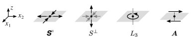
Figure 4: Singularity diagrams corresponding to each of the terms in 36. Arrows indicate distributions of point forces or torques and the gray shaded region indicates the interface.

Each term in 36 makes a distinct contribution to the interfacial dipole moment. We call each contribution by its (tensorial) prefactor and graphically represent them as distributions of Stokes singularities in figure 4. The $\boldsymbol{\mathsfbi{S}}^{\shortparallel}$ mode, given by 37a, is a viscosity-averaged stresslet associated with extensional stresses produced by the colloid in the interfacial plane. Similarly, the $S^{\perp}$ mode, given by 37b, is the viscosity-averaged stresslet perpendicular to the interface. Furthermore, $\mathsfi S^{(\nu)}_{33}=-\mathsfi S^{(\nu)}_{11}-\mathsfi S^{(\nu)}_{22}$ because $\boldsymbol{\mathsfbi{S}}^{(\nu)}$ is traceless, so $S^{\perp}$ accounts for extensional stress perpendicular to the interface and planar compression of the interface. The $L_{3}$ mode in 36 is a viscosity-averaged rotlet, or point torque, about the $z$ axis of strength $L_{3}$. These viscosity-averaged flows exhibit mirror symmetry of the velocity field about $z=0$. Therefore, the tangential shear stress due to these modes vanishes on the interface, as is the case for the monopole moment.

The $\boldsymbol{A}$ mode corresponds to a force dipole where the forces act parallel to the interface and are displaced from one another along the axis normal to the interface. This mode does not produce a viscosity-averaged flow. Instead, the flow speed in one phase differs from that in the opposite phase by a factor of the viscosity ratio; intuitively, the flow is slower in the more viscous phase. On the interface, the fluid velocity vanishes. We see from the last term of 36 that the flows in the upper and lower half spaces are equivalent to effective stresslets in an unbounded fluid for $z>0$ and $z<0$, respectively.

Quadrupolar and higher-order terms of 27 can be similarly decomposed into two subsets of modes; one whose tangential stress vanishes at the interface and another whose velocity vanishes at the interface. Members of the former subset are mirror-symmetric, viscosity-averaged flows and the latter have velocities that differ by in magnitude by the viscosity ratio on either side of the interface. We do not detail the higher-order modes further. The force monopole 29 and force dipole 36 describe the leading-order flows due to driven and active colloids, respectively. In many cases, we can infer these modes based on the geometry of a given colloidal particle and its configuration with respect to the interface.

4.4 Discussion

4.4.1 Driven colloids

For colloids driven by an external force $\boldsymbol{F}_{\text{ext}}$ with a non-zero component parallel to the interface, the monopole moment—a viscosity averaged Stokeslet—is the leading-order far-field flow. The strength of this effective Stokeslet is simply $\boldsymbol{\mathsfbi{I}}_{\mathrm{s}}\boldsymbol{\cdot}\boldsymbol{F}_{\text{ext}}$, regardless of whether the colloid is adhered or adjacent to the interface. An interesting special case occurs when $\boldsymbol{F}_{\text{ext}}$ acts purely perpendicular to the interface. For an adhered colloid, this force generates no motion of the colloid—or the fluid—due to the pinned contact line. However, motion will result if the colloid is instead adjacent to the interface. In this case, $\boldsymbol{u}^{\text{m}0}$ still vanishes by 29, so the dipole becomes the leading-order mode. For instance, consider a colloid fully immersed in fluid 1 whose center is located a small distance $\delta$ from the interface. This colloid is acted upon by the force $\boldsymbol{F}_{\text{ext}}=F_{3}\hat{\boldsymbol{\imath}}_{3}$, which drives it in rigid-body motion. Recall that we have expanded $\boldsymbol{u}$ into multipoles with respect to the origin point $\boldsymbol{0}$ on the interface, and each multipole prefactor is therefore ‘measured’ with respect to this point. Letting $\boldsymbol{y}=\boldsymbol{y}^{\prime}+\delta\hat{\boldsymbol{\imath}}_{3}$ in 30, where $\boldsymbol{y}^{\prime}$ is the displacement vector from the center of the colloid, we find

$$\boldsymbol{\mathsfbi{D}}^{(1)}=-\int_{S_{1}}(\boldsymbol{\mathsfbi{\sigma}}\boldsymbol{\cdot}\hat{\boldsymbol{n}})(\boldsymbol{y}^{\prime}+\delta\hat{\boldsymbol{\imath}}_{3})\mathop{}\!\mathrm{d}{S}(\boldsymbol{y}^{\prime})=\boldsymbol{\mathsfbi{D}}_{\text{c}}+\delta F_{3}\hat{\boldsymbol{\imath}}_{3}\hat{\boldsymbol{\imath}}_{3},$$ (38)

where $\boldsymbol{\mathsfbi{\mathsfi}}D_{\text{c}}$ is the dipole strength as measured from the colloid center. Thus, the external force on the colloid contributes a factor of $\delta F_{3}\hat{\boldsymbol{\imath}}_{3}\hat{\boldsymbol{\imath}}_{3}$ to $\boldsymbol{\mathsfbi{D}}^{(1)}$ (or a factor of $\delta F_{3}$ to $S^{\perp}$). If the characteristic size of the colloid $a$ is small compared with $\delta$, then we expect $\delta F_{3}\gg|\boldsymbol{\mathsfbi{\mathsfi}}D_{\text{c}}|$. Otherwise, when $\delta\sim a$, contributions from $\boldsymbol{\mathsfbi{D}}_{\text{c}}$ are generally significant and are sensitive to particle geometry, its distance to the interface, and the viscosity ratio.

An external torque $\boldsymbol{L}_{\text{ext}}$ on the colloid also drives flow. First, consider a torque about the $z$-axis, $\boldsymbol{L}_{\text{ext}}=L_{\text{ext},3}\hat{\boldsymbol{\imath}}_{3}$. This torque is balanced hydrodynamically whether or not the colloid is adhered to the interface because the contact line does not resist rotation about the $z$ axis. Thus, $L_{3}=L_{\text{ext},3}$. The $L_{3}$ mode of 36 induces a viscosity-averaged rotlet. For colloids that are axisymmetric about the $z$-axis, this is the only non-vanishing mode of 36; it is readily shown that, in this case, $\mathsfi S^{\shortparallel}_{jk}=S^{\perp}=A_{\alpha}=0$. For general colloid geometries, these coefficients are generally non-zero, so an external torque potentially produces all of the modes represented by 36. We may also consider an external torque parallel to the interface. If the colloid is adhered to the interface, this torque does not produce flow due to the pinned contact line. For an adjacent colloid immersed in either fluid, the colloid is able to rotate, and we see from 37c that the $\boldsymbol{A}$ mode is produced. This mode may be accompanied by other dipolar modes that are linearly coupled to the resulting motion of the colloid.

4.4.2 Active colloids

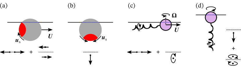
Figure 5: We depict some examples of active colloids at interfaces. Panels (a,b) illustrate an active colloidal particle adhered to an interface, which possesses an active cap that generates a phoretic slip velocity $\boldsymbol{u}_{\mathrm{s}}$ along its surface. In (a), the horizontal particle orientation leads to in-plane swimming at velocity $\boldsymbol{U}$. In (b), the same active particle is adhered vertically to the interface as to instead ‘pump’ fluid. Here, the particle cannot reorient to swim forward due to a pinned contact line. Panels (c,d) illustrate a bacterium also in swimming and pumping configurations. Thrust is generated by a rotating flagellum, which also produces a torque. In (c), this torque is balanced by contact-line pinning, so there is a net hydrodynamic torque exerted on the fluid below the interface. For the vertically adhered bacterium (d), the hydrodynamic torque on the upper and lower fluid must vanish, since the body of the bacterium is free to counterrotate about the $z$ axis. The singularity diagrams next to each illustration give minimal “point-force” models describing to the leading-order flows these active colloids are expected to generate. The arrows represent the orientation of these forces or torques (circular arrows) relative to the interface (dashed line).

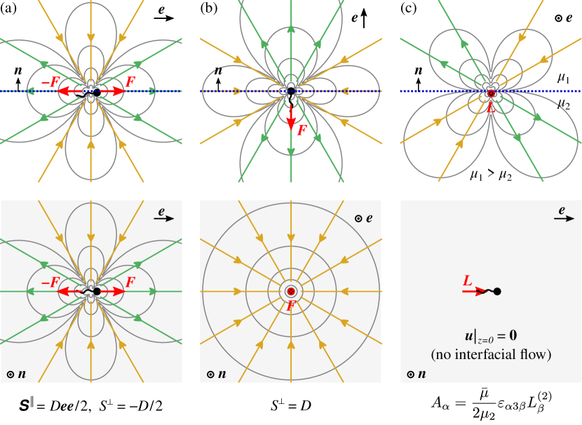
Figure 6: Dipolar hydrodynamic modes for an active colloid at a clean interface. The upper panels are side views that depict the flow in a cross-section intersecting the colloid, in which the blue dotted line indicates the location of the interface. The lower panels are top-down views of the same flows on the interface. Forms of the prefactors from 36 associated with each mode are indicated at the bottom. The streamlines indicate the flow disturbance due to the colloid, and the gray lines are contours of constant $|\boldsymbol{u}|$. The vector $\boldsymbol{e}$ represents the alignment of the swimmer. (a) Force dipole (stresslet) mode expected for a swimmer moving parallel to the interface. The configuration of the swimmer is like that in figure 5(a) or (c). (b) Stresslet due to an active colloid pinned at the interface, with a configuration as illustrated in figure 5(b) or (d). Modes (a,b) are the same as the force dipole in a bulk fluid with viscosity $\bar{\mu}$ and are axisymmetric about the swimmer alignment axis. (c) Flow due to a point torque $\boldsymbol{L}$ on the lower fluid, just below the interface, where $\boldsymbol{L}$ is parallel to the interface. Such a flow is expected for certain active colloids such as the bacterium illustrated in figure 5(c). This mode is associated with asymmetry in the activity and/or geometry of the colloid about the interfacial plane, as detailed in section 4.4.3.

Active colloids self-propel absent external forces or torques. For many kinds of active colloids, self-propulsion is generated by some active, thrust-producing part of the colloid that drives the remaining passive part, as illustrated in figure 5; spatial separation of thrust and drag on the object generate a hydrodynamic dipole. Therefore, in a bulk fluid, an appropriate far-field model of an active colloid is that of a stresslet along the axis of swimming (Lauga & Powers, 2009), which produces the velocity field

$$\boldsymbol{u}^{\text{S}}(\boldsymbol{e};\boldsymbol{x})=-\frac{D}{\mu_{\text{b}}}\boldsymbol{e}(\boldsymbol{e}\boldsymbol{\cdot}\boldsymbol{\nabla})\boldsymbol{\mathsfbi{J}}(\boldsymbol{x}),$$ (39)

where $D$ is the strength of the force dipole, $\mu_{\text{b}}$ is the viscosity of the bulk fluid, and $\boldsymbol{e}$ is a unit vector indicating the swimmer alignment. A similar model is sensible for an active colloid swimming parallel to the interface as illustrated in figure 5(a,c). Indeed, the same velocity field as 39 is produced by setting $\boldsymbol{\mathsfbi{S}}^{\shortparallel}=D\boldsymbol{e}\boldsymbol{e}/2$ and $S^{\perp}=-D/2$ in 36, with $\bar{\mu}$ replacing $\mu_{\text{b}}$. The resulting flow profile is illustrated in figure 6a.

By instead setting $S^{\perp}=D$ and $\boldsymbol{\mathsfbi{S}}^{\shortparallel}=\boldsymbol{0}$ in 36, one obtains the same flow profile albeit rotated by $90\text{\,}\mathrm{\SIUnitSymbolDegree}$. This pure-$S^{\perp}$ mode is expected of active colloids trapped perpendicular to the interface, $\boldsymbol{e}=\boldsymbol{n}$, as depicted in figure 5(b,d). The colloid cannot self-propel in this configuration due to the pinned contact line, so the apparent stresslet 39 is not due to balancing hydrodynamic thrust and drag. Instead of swimming, the colloid becomes a fluid pump, resulting in a non-zero net hydrodynamic force on the colloid that is balanced by capillary forces. A minimal model for this pumping configuration is that of a point force exerted along the $z$ axis a small distance $\delta$ from the interface. While the monopole moment vanishes for a force in this direction, the dipole moment does not due to the small but finite separation of the force from the interface. The vertical point force gives $S^{\perp}=F\delta$ in 36, which is associated with the flow plotted in figure 6b. Viewed in the interfacial plane, this flow is sink like for a pusher ($S^{\perp}>0$) and source like for a puller ($S^{\perp}<0$). A pusher causes surface expansion ($\boldsymbol{\nabla}_{\!\mathrm{s}}\boldsymbol{\cdot}\boldsymbol{u}>0$), as new interface must be created to replace the ‘sink.’ Conversely, a puller causes surface compression.

Another unique feature of active colloids adhered to interfaces is that they may exert a net hydrodynamic torque on the fluid about an axis parallel to the interface. This torque is balanced by capillary forces at the contact line. Figure 5c illustrates this scenario for a motile bacterium adhered to the interface by its body and propelled by a rotating flagellum. The effect of this torque on the far-field flow enters through the coefficient $\boldsymbol{A}$ in 36. The resulting flow profile is shown in figure 6c. The presence of this mode potentially discriminates the far-field flow of adhered versus unadhered swimmers; the net torque must vanish for active colloids that are adjacent but not adhered to the interface. In the case of an adjacent bacterium, counterrotation of the body and flagellum instead produce a torque dipole in the far-field, a member of the higher-order quadrupole moment. A perpendicular configuration of the bacterium, as in figure 5(d) produces a torque dipole as well because the body may freely counterrotate in in the interface. As discussed further below, this mode is of particular interest in advective mixing near fluid interfaces, regardless of interfacial mechanics.

4.4.3 Symmetry and asymmetry about the interfacial plane

To conclude this discussion, we return to the motif of two major categories of modes: those which are weighted by the average viscosity, with vanishing tangential stress at the interface, and those whose flow speed on either side of the interface differs by a factor of the viscosity ratio, with vanishing velocity on the interface. To dipolar order, only the $\boldsymbol{A}$ mode in 36 falls into the latter category. The previous discussion associated $\boldsymbol{A}$ with a net hydrodynamic torque on the fluid adjacent to the interface about an axis parallel to the interface. Such torques might arise from active stresses or, for colloids adjacent to the interface, a driving external torque. However, this mode is not uniquely associated with these torques; from 37c, we see that it also involves the components of the stresslet $\mathsfi S^{(\nu)}_{\alpha 3}$.

To gain a better understanding of the $\boldsymbol{A}$ mode, consider a spherical colloid of radius $a$ that is adhered to the interface with a $90\text{\,}\mathrm{\SIUnitSymbolDegree}$ contact angle, such that half of the sphere is in each fluid. We may exactly obtain the flow due to rigid-body motion of this sphere by referencing an auxiliary problem where the sphere instead moves through a fluid of uniform viscosity $\bar{\mu}$ (Ranger, 1978; Pozrikidis, 2007). If the sphere translates at velocity $\boldsymbol{U}$ in the $z=0$ plane and rotates with angular velocity $\hat{\boldsymbol{\imath}}_{3}\Omega_{3}$, the fluid velocity in the laboratory frame with its origin at the center of the sphere is

$$\boldsymbol{u}(\boldsymbol{x})=\boldsymbol{F}\left(1+\frac{a^{2}}{6}\nabla^{2}\right)\boldsymbol{\cdot}\boldsymbol{\mathsfbi{J}}(\boldsymbol{x})+\frac{1}{2}L_{3}\hat{\boldsymbol{\imath}}_{3}\boldsymbol{\cdot}[\boldsymbol{\nabla}\times\boldsymbol{\mathsfbi{J}}(\boldsymbol{x})],$$ (40)

where $\boldsymbol{F}=6\upi\bar{\mu}\boldsymbol{U}a$ is the Stokes drag and $L_{3}=8\upi\bar{\mu}\Omega_{3}$ is the torque. This velocity field is mirror symmetric about the $z=0$ plane, so the tangential stress vanishes on $z=0$. It follows that 40 trivially satisfies 3 and is therefore also the solution for two fluids of differing viscosities that average to $\bar{\mu}$; the flow is independent of the viscosity contrast. There is a normal stress jump across the interface in this case, but it is inconsequential at small $\mathinner{Ca}$, where the interface remains nearly flat.

The first term of 40 comprises a viscosity-averaged Stokeslet and degenerate quadrupole (or source doublet) at the center of the sphere. Thus, for the sphere described above, the dipole moment vanishes, excepting the viscosity-averaged rotlet described by the $L_{3}$ mode of 36. If there is no external torque on the sphere but it translates along, e.g., the $x$ axis, then we expect a non-zero hydrodynamic torque about the $y$ axis unless $\mu_{1}=\mu_{2}$. One might naively expect this hydrodynamic torque to produce flow, which clearly contributes to $\boldsymbol{A}$ in 37c. However, for the velocity field produced by a sphere, the $\boldsymbol{\mathsfbi{S}}^{(\nu)}$ contribution to $\boldsymbol{A}$ exactly cancels that from $\boldsymbol{L}^{(\nu)}$ due to the sphere’s symmetry about the interfacial plane.

More generally, we expect a viscosity-averaged flow to result for any driven or active colloid with mirror symmetry about $z=0$. If the boundary motion is symmetric about $z=0$, then the resulting fluid flow will reflect this symmetry. Thus, the $\boldsymbol{A}$ mode only contributes to the flow when there is some degree of asymmetry. For rigid, driven colloids, this asymmetry may come from an asymmetric colloid shape or adhered configuration with the interface (for a sphere, a contact angle other than $90\text{\,}\mathrm{\SIUnitSymbolDegree}$). For active colloids, there will likely be asymmetry in activity or boundary motion, especially if the two fluid phases have differing viscosities or chemical properties. For example, the phoretic swimmer illustrated in figure 5a is expected to produce a leading-order stresslet parallel to the interface due to hydrodynamic thrust and drag (figure 6a). However, we also expect a contribution from the asymmetric mode illustrated by figure 6c. In experiment, contact-line pinning fixes colloids in random configurations at fluid interfaces, so such asymmetric adhered states are likely the norm.

5 Incompressible interfaces and the role of surface viscosity

As discussed in section 2.3, fluid interfaces are typically incompressible due to the inevitable presence of surface-active impurities. Because materials accumulate at interfaces, they often act as two-dimensional fluids with their own rheology. Here, we address incompressible interfaces with zero and finite shear viscosities.

5.1 Green’s function

We may define a Green’s function $\boldsymbol{\mathsfbi{H}}$ for an incompressible interface that is analogous to that discussed in section 4.1 for a clean interface. The major difference is that the interfacial stress balance 17a is replaced by

$$-\boldsymbol{\nabla}_{\!\mathrm{s}}\boldsymbol{\Pi}+\mu_{\mathrm{s}}\nabla_{\!\mathrm{s}}^{2}\boldsymbol{\mathsfbi{H}}+\boldsymbol{\mathsfbi{I}}_{\mathrm{s}}\boldsymbol{\cdot}{\left[\boldsymbol{n}\boldsymbol{\cdot}\boldsymbol{\mathsfbi{T}}(\boldsymbol{\mathsfbi{H}};\!)\right]}_{I} =\begin{cases}-\boldsymbol{\mathsfbi{I}}_{\mathrm{s}}\delta_{\mathbb{R}^{2}}(\boldsymbol{x}-\boldsymbol{y})&h=0\\ \boldsymbol{0}&h\neq 0\end{cases}$$ (41a)

$$\boldsymbol{\nabla}_{\!\mathrm{s}}\boldsymbol{\cdot}\boldsymbol{\mathsfbi{H}} =0,$$ (41b)

where $\boldsymbol{\mathsfbi{\Pi}}$ is the (vectorial) surface pressure associated with $\boldsymbol{\mathsfbi{H}}$, which enforces the surface incompressibility constraint 41b. Thus, $\boldsymbol{\mathsfbi{H}}$ satisfies 16 subject to 17b and 41, with $\boldsymbol{\mathsfbi{G}}$ replaced by $\boldsymbol{\mathsfbi{H}}$ in the former two equations. The coupling of bulk-viscous and surface-viscous effects induce a natural length scale in the problem, the Boussinesq length, which is given by $L_{\text{B}}=\mu_{\mathrm{s}}/\bar{\mu}$. Bulk-viscous dissipation dominates at distances $r\gg L_{\text{B}}$, and surface-viscous dissipation dominates when $r\ll L_{\text{B}}$. It is therefore convenient to define the dimensionless Boussinesq number, $\mathinner{Bq}=L_{\text{B}}/a$, which quantifies the relative importance of surface-viscous to bulk-viscous effects for a colloid of characteristic size $a$.

The functional form of $\boldsymbol{\mathsfbi{H}}$, derived in full by Bławzdziewicz et al. (1999), is more complicated than that of $\boldsymbol{\mathsfbi{G}}$ owing to non-trivial interfacial stress balance 41. However, like $\boldsymbol{\mathsfbi{G}}$, $\boldsymbol{\mathsfbi{H}}$ is self-adjoint (see appendix A) and therefore satisfies

$$\boldsymbol{\mathsfbi{H}}(\boldsymbol{x},\boldsymbol{y})=\boldsymbol{\mathsfbi{H}}^{\mathsf{T}}(\boldsymbol{y},\boldsymbol{x}).$$ (42)

We may use this property to determine the multipole expansion at points on the interface requiring only knowledge of $\boldsymbol{\mathsfbi{H}}(\boldsymbol{x},\boldsymbol{y})$ for $\boldsymbol{y}\in I$, in addition to the previously determined expansion for a clean interface. Letting $\boldsymbol{\mathsfbi{H}}^{0}(\boldsymbol{s},z)=\boldsymbol{\mathsfbi{H}}(\boldsymbol{x},\boldsymbol{0})$, we find that for a fixed value of $L_{\text{B}}$ (see appendix B for derivation)

$$\mathsfi H^{0}_{\alpha\beta}(\boldsymbol{s},z)=\frac{1}{4\upi\bar{\mu}}R_{0}(L_{\text{B}};s,|z|)\delta_{\alpha\beta}+\frac{1}{2\upi\bar{\mu}}R_{2}(L_{\text{B}};s,|z|)\left\{\hat{s}_{\alpha}\hat{s}_{\beta}\right\}_{0}$$ (43)

and $\mathsfi H^{0}_{3i}=\mathsfi H^{0}_{i3}=0$, where $\boldsymbol{s}=\boldsymbol{\mathsfbi{I}}_{\mathrm{s}}\boldsymbol{\cdot}\boldsymbol{x}=x_{1}\hat{\boldsymbol{\imath}}_{1}+x_{2}\hat{\boldsymbol{\imath}}_{2}$, $s=|\boldsymbol{s}|$, $\hat{\boldsymbol{s}}=|\boldsymbol{s}|/s$, and $\left\{\cdot\right\}_{0}$ denotes the irreducible (traceless, symmetric) part of the enclosed tensor. Here, e.g., $\left\{\hat{s}_{\alpha}\hat{s}_{\beta}\right\}_{0}=\hat{s}_{\alpha}\hat{s}_{\beta}-\frac{1}{2}\delta_{\alpha\beta}$, where we regard $\hat{\boldsymbol{s}}$ as a two dimensional vector and the $\{\cdot\}_{0}$ operation as being on a two-dimensional tensor. The functions $R_{0}$ and $R_{2}$, given by 93, depend only on the magnitudes of $\boldsymbol{s}$ and $z$. Equation 42 equips $\boldsymbol{\mathsfbi{H}}^{0}$ with dual interpretations; $\mathsfi H^{0}_{ij}(\boldsymbol{s},z)\,F_{j}$ is the velocity field due to the point force $\boldsymbol{F}$ on the interface at $\boldsymbol{y}=\boldsymbol{0}$, and $\mathsfi H^{0}_{ij}(\boldsymbol{s},h)\,F_{j}$ is the velocity field on the interface induced by the same point force exerted at $\boldsymbol{y}=h\hat{\boldsymbol{\imath}}_{3}$ (within either of the fluids).

The velocity field represented by $\boldsymbol{\mathsfbi{H}}^{0}(\boldsymbol{s},z)$ is everywhere parallel to the interface. As noted by Stone & Masoud (2015), this feature is generally expected of Stokes flow driven by arbitrary motion of an incompressible plane. The $z$ velocities of the fluids vanish at the interface as do their $z$ derivatives due to the incompressibility of the interface and the surrounding fluids. These quantities also vanish as $|\boldsymbol{x}|\to\infty$. As a Stokes flow, $\boldsymbol{u}$ is biharmonic, and hence $\nabla^{4}u_{3}=0$. It follows from the homogeneous behavior of $u_{3}$ on the interface and at infinity that $u_{3}=0$ everywhere. The vanishing behavior of $\mathsfi H^{0}_{3j}$ reflects this property.

When the interface is inviscid, $L_{\text{B}}=0$, $R_{n}$ admits the closed form given by 94, and 43 reduces to

$${\left.\mathsfi H^{0}_{\alpha\beta}\right|}_{L_{\text{B}}=0}=\frac{\delta_{\alpha\beta}}{8\upi\bar{\mu}r}+\frac{(r-|z|)^{2}}{4\upi\bar{\mu}rs^{2}}\left\{\hat{s}_{\alpha}\hat{s}_{\beta}\right\}_{0}.$$ (44)

Thus, Marangoni stresses alone do not change the $r^{-1}$ rate of decay of the fluid velocity from the singular point at the origin found for a clean interface. The flow on the interface is purely radial and is given by

$${\left.\mathsfi H^{0}_{\alpha\beta}(\boldsymbol{x}\in I)\right|}_{\mathinner{Bq}=0}=\frac{\hat{s}_{\alpha}\hat{s}_{\beta}}{8\upi\bar{\mu}r}.$$

For finite $L_{\text{B}}$, $\boldsymbol{\mathsfbi{H}}$ approaches the form given by 44 for $r\gg L_{\text{B}}$. In the opposite limit where $L_{\text{B}}\to\infty$, we recover the equations governing a two-dimensional Stokes flow from 41, as viscous stresses from the two fluid phases become negligible. Therefore, $\boldsymbol{\mathsfbi{H}}^{0}$ coincides with a Stokeslet in a two dimensional fluid (up to an arbitrary constant) (Saffman & Delbrück, 1975),

$${\left.\mathsfi H^{0}_{\alpha\beta}\right|}_{L_{\text{B}}\to\infty}\sim\frac{\hat{s}_{\alpha}\hat{s}_{\beta}-\delta_{\alpha\beta}\ln s}{4\pi\mu_{\mathrm{s}}},$$ (45)

which is constant in $z$ (as a three-dimensional flow field) and diverges logarithmically as $s$ is made large. For finite $L_{\text{B}}$, $\boldsymbol{\mathsfbi{H}}$ approaches the form given by 45 for $r\ll L_{\text{B}}$. Clearly, 45 does not satisfy the homogeneous boundary conditions imposed on $\boldsymbol{\mathsfbi{H}}$ as $r\to\infty$. Of course, this is Stokes’ paradox; for large but finite $L_{\text{B}}$, 45 is not valid for $r\gtrsim L_{\text{B}}$, where bulk-viscous effects inevitably become important. Returning to the general expression 43, we find that the $R_{n}$ functions transition the flow field between the surface-viscosity-dominated, logarithmically divergent behavior at distances $r\ll L_{\text{B}}$ from the colloid to the convergent, $1/r$ decay at distances $r\gg L_{\text{B}}$, where surface viscosity has a negligible effect.

The surface pressure $\boldsymbol{\Pi}=\boldsymbol{\Pi}(\boldsymbol{x},\boldsymbol{y})$ associated with $\boldsymbol{\mathsfbi{H}}(\boldsymbol{x},\boldsymbol{y})$ is independent of $L_{\text{B}}$, as has been previously found (Bławzdziewicz et al., 1999; Fischer et al., 2006), and is given in our notation by (see appendix B for derivation)

$$\Pi_{i}(\boldsymbol{s},h\hat{\boldsymbol{\imath}}_{3})=\frac{s_{i}}{4\upi s^{2}}{\left(1-\frac{|h|}{\sqrt{s^{2}+h^{2}}}\right)}-\frac{|h|(s_{i}-hn_{i})}{4\upi{(s^{2}+h^{2})}^{3/2}}.$$ (46)

Equation 46 shows that $|\boldsymbol{\mathsfbi{\Pi}}|\sim 1/s$ for $h$ fixed and $s\gg h$, and $|\boldsymbol{\mathsfbi{\Pi}}|\sim 1/h$ for $s$ fixed and $h\gg s$. For $h=0$, 46 reduces to the harmonic pressure field $\boldsymbol{\mathsfbi{\Pi}}(\boldsymbol{s},\boldsymbol{0})=\boldsymbol{s}/4\upi s^{2}$.

5.2 Multipole expansion

5.2.1 Expansion of the boundary integral equation

Using the reciprocal relation 15 for two fluids separated by an incompressible interface and following a procedure similar to that described in section 4.2, we obtain the boundary integral representation for $\boldsymbol{u}(\boldsymbol{x})$ as

$$u_{k}(\boldsymbol{x})=-\oint_{S_{\text{c}}}{\mathsfi H_{kj}(\boldsymbol{x},\boldsymbol{y})\,[\hat{n}_{i}\sigma_{ij}](\boldsymbol{y})}\mathop{}\!\mathrm{d}S(\boldsymbol{y})+\oint_{S_{\text{c}}}{[\hat{n}_{i}u_{j}](\boldsymbol{y})\,\mathsfi T_{ijk}(\boldsymbol{\mathsfbi{H}};\boldsymbol{y},\boldsymbol{x})}\mathop{}\!\mathrm{d}S(\boldsymbol{y})\\ -\oint_{C}{\mathsfi H_{k\beta}(\boldsymbol{x},\boldsymbol{y})\,[\hat{m}_{\alpha}\varsigma_{\alpha\beta}](\boldsymbol{y})}\mathop{}\!\mathrm{d}C(\boldsymbol{y})+\oint_{C}{[\hat{m}_{\alpha}u_{\beta}](\boldsymbol{y})\,\Sigma_{\alpha\beta k}(\boldsymbol{\mathsfbi{H}};\boldsymbol{y},\boldsymbol{x})}\mathop{}\!\mathrm{d}C(\boldsymbol{y}),$$ (47)

where $\hat{\boldsymbol{m}}=\hat{\boldsymbol{\imath}}_{3}\times\hat{\boldsymbol{t}}$, $C$ is the curve in the $z=0$ plane that runs along the three-phase contact line (see figure 2), and $\boldsymbol{\mathsfbi{\Sigma}}(\boldsymbol{\mathsfbi{H}};\!)$ is the surface stress tensor associated with $\boldsymbol{\mathsfbi{H}}$, which is given by

$$\Sigma_{\alpha\beta k}(\boldsymbol{\mathsfbi{H}};\boldsymbol{y},\boldsymbol{x})=-\delta^{\shortparallel}_{\alpha\beta}\Pi_{k}(\boldsymbol{y},\boldsymbol{x})+\mu_{s}\left(\frac{\partial\mathsfi H_{k\beta}(\boldsymbol{x},\boldsymbol{y})}{\partial y_{\alpha}}+\frac{\partial\mathsfi H_{k\alpha}(\boldsymbol{x},\boldsymbol{y})}{\partial y_{\beta}}\right)$$

for $\boldsymbol{y}\in I$. Equation 47 is valid as long as $L_{\text{B}}$ is finite. We require the $1/r$ spatial decay of $\boldsymbol{\mathsfbi{H}}$ at distances $r\gg L_{B}$ from the colloid for the integrals in this equation to converge unconditionally. Comparing 47 to 24, the last two terms of 47 are new and account for Marangoni forces and surface-viscous stresses at the contact line, respectively.

As before, we may generate a multipole expansion for $\boldsymbol{u}(\boldsymbol{x})$ by replacing $\boldsymbol{\mathsfbi{H}}$, $\boldsymbol{\mathsfbi{T}}(\boldsymbol{\mathsfbi{H}};\!)$, and $\boldsymbol{\mathsfbi{\Sigma}}(\boldsymbol{\mathsfbi{H}};\!)$ in 47 with their respective Taylor series about $\boldsymbol{y}=\boldsymbol{0}$, where $\boldsymbol{0}$ is placed at an appropriate point on the interface. We may write the expansion as $\boldsymbol{u}=\boldsymbol{u}^{(1)}+\boldsymbol{u}^{(2)}+\boldsymbol{u}^{(\text{i})}$, where

$$\boldsymbol{u}^{(1)} =\text{same as right-hand side of \lx@cref{creftype~refnum}{eq:mpx-clean-upper} with $\boldsymbol{\mathsfbi{G}}$ replaced by $\boldsymbol{\mathsfbi{H}}$,}$$ (48)

$$\boldsymbol{u}^{(2)} =\text{same as right-hand side of \lx@cref{creftype~refnum}{eq:mpx-clean-lower} with $\boldsymbol{\mathsfbi{G}}$ replaced by $\boldsymbol{\mathsfbi{H}}$,}$$ (49)

and

$$u^{(\text{i})}_{k}(\boldsymbol{x})=- \sum_{n=0}^{\infty}{\frac{1}{n!}\left(\int_{C}[\hat{m}_{\alpha}\varsigma_{\alpha\beta}](\boldsymbol{y})\,y_{\gamma_{1}}\cdots y_{\gamma_{n}}\mathop{}\!\mathrm{d}C(\boldsymbol{y})\right)\left.\frac{\partial^{n}\mathsfi H_{k\beta}(\boldsymbol{x},\boldsymbol{y}\in I)}{\partial y_{\gamma_{1}}\cdots\partial y_{\gamma_{n}}}\right|_{\boldsymbol{y}=\boldsymbol{0}}}$$ (50)

$$+ \sum_{n=0}^{\infty}{\frac{1}{n!}\left(\int_{C}[u_{\beta}\hat{m}_{\alpha}](\boldsymbol{y})\,y_{\gamma_{1}}\cdots y_{\gamma_{n}}\mathop{}\!\mathrm{d}C(\boldsymbol{y})\right)\left.\frac{\partial^{n}\Sigma_{\alpha\beta k}(\boldsymbol{\mathsfbi{H}};\boldsymbol{y}\in I,\boldsymbol{x})}{\partial y_{\gamma_{1}}\cdots\partial y_{\gamma_{n}}}\right|_{\boldsymbol{y}=\boldsymbol{0}}}.$$

Collecting terms from 48, 49 and 50, we may write $\boldsymbol{u}$ as a multipole expansion analogous to that given by 26,

$$\boldsymbol{u}(\boldsymbol{x})=\boldsymbol{u}^{\text{m0}}(\boldsymbol{x})+\boldsymbol{u}^{\text{m1}}(\boldsymbol{x})+\boldsymbol{u}^{\text{m2}}(\boldsymbol{x})+\text{h.o.t},$$ (51)

where

$$u^{\text{m0}}_{i}(\boldsymbol{x}) =F^{(1)}_{j}\mathsfi H_{ij}(\boldsymbol{x},\boldsymbol{0}^{+})+F^{(2)}_{j}\mathsfi H_{ij}(\boldsymbol{x},\boldsymbol{0}^{-})+F^{(\text{i})}_{\beta}\mathsfi H_{i\beta}(\boldsymbol{x},\boldsymbol{0})$$ (51a)

$$u^{\text{m1}}_{i}(\boldsymbol{x}) =\mathsfi D^{(1)}_{jk}\frac{\partial\mathsfi H_{ij}}{\partial y_{k}}(\boldsymbol{x},\boldsymbol{0}^{+})+\mathsfi D^{(2)}_{jk}\frac{\partial\mathsfi H_{ij}}{\partial y_{k}}(\boldsymbol{x},\boldsymbol{0}^{-})+\mathsfi D^{(\text{i})}_{\beta\gamma}\frac{\partial\mathsfi H_{i\beta}}{\partial y_{\gamma}}(\boldsymbol{x},\boldsymbol{0}).$$ (51b)

Equations 51a and 51b are analogous to 27a and 27b, respectively, and each of these equations contain an additional term that accounts for stresses exerted by the colloid on the interface. Equation 51b assumes that the hole in the interface created by the colloid is of constant surface area and that the volume of the colloid is also constant.

5.2.2 Monopole Moment

At an incompressible interface, the monopole moment retains its interpretation as the leading-order flow due to a colloid that is driven by an external force. Indeed, $\boldsymbol{\mathsfbi{H}}(\boldsymbol{x},\boldsymbol{y})$ is continuous as $\boldsymbol{y}$ is moved across the interface, so ${\boldsymbol{u}}^{\text{m0}}(\boldsymbol{x})$ reduces to

$$u^{\text{m0}}_{i}(\boldsymbol{x})=F_{j}\mathsfi H^{0}_{ij}(\boldsymbol{x})=\left(F^{(1)}_{j}+F^{(2)}_{j}+F^{(\text{i})}_{\beta}\delta^{\shortparallel}_{\beta j}\right)\mathsfi H^{0}_{ij}(\boldsymbol{x}),$$ (52)

where $\boldsymbol{F}$ is the total force exerted on the surrounding system: the two fluids and the interface. Compared with the analogous expression for a clean interface 29, the surface-incompressible monopole has the additional contribution to its prefactor given by $F^{(\text{i})}_{\beta}=-\oint_{C}\hat{m}_{\alpha}\varsigma_{\alpha\beta}\mathop{}\!\mathrm{d}C,$ which is the force exerted on the interface by the colloid at the contact line due to Marangoni and surface-viscous stresses. Like the clean-interface monopole, the surface-incompressible monopole given by 52 is independent of the viscosity contrast between the two fluids and is mirror symmetric with respect to the $z=0$ plane. However, the surface-incompressible monopole lacks the axisymmetry of its clean-interface analogue. From 52, we find that $\boldsymbol{u}^{\text{m0}}$ only contributes to velocity components parallel to the interface because $\mathsfi H^{0}_{i3}=0$. Hence, this mode is associated with ‘lamellar’ fluid motion, a feature not shared with its clean-interface analogue.

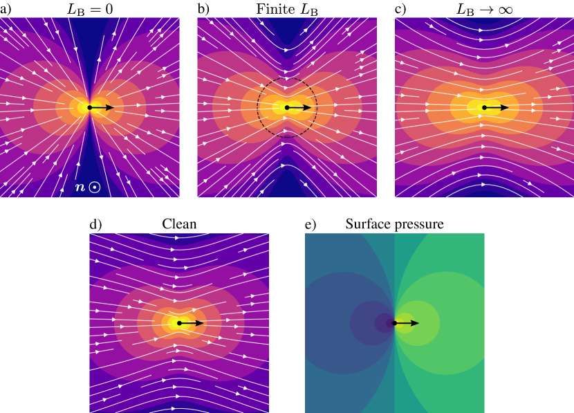
Figure 7: The velocity field on the interfacial plane due to a surface-incompressible force monopole is shown for different values of $L_{\text{B}}$ (a-c). The result for a clean interface (d) is also shown for comparison. In (b), the distance $r=L_{\text{B}}$ is indicated by the dashed circle. The arrows show the location and direction of the point of forcing. The surface pressure profile (e) associated with (a-c) is independent of $L_{\text{B}}$. The logarithmically spaced contours correspond to velocity magnitude (a-d) and surface pressure (e), where lighter colored contours indicate larger values and darker colors approach zero. Panels (a), (b), and (c), represent the leading-order velocity fields due to a colloid driven by an external force for small-, moderate-, and large-$\mathinner{Bq}$, respectively.

Figure 7 shows the interfacial velocity and surface pressure profiles of the force monopole 52. For $L_{\text{B}}=0$ (figure 7a), the flow is quite different than that for a clean interface (figure 7d), although in both cases the velocity magnitude decays as $1/r$. Here, the flow is modified from that at a clean interface by Marangoni stresses alone. Figure 7a is representative of the leading-order flow for a driven colloid whose characteristic size far exceeds $L_{\text{B}}$ ($\mathinner{Bq}\ll 1$), where surface-viscous forces are weak everywhere on the interface. The moderate-$\mathinner{Bq}$ case is shown in figure 7b. The more complicated flow pattern owes to the interplay between bulk-viscous, surface-viscous, and Marangoni stresses, which are all comparable in magnitude for $r\sim L_{\text{B}}$. Figure 7c shows the large-$\mathinner{Bq}$ regime, where dissipation is dominated by the surface viscosity except at very large distances of $r\geq O(a\mathinner{Bq})$. For smaller $O(a)$ distances, the flow profile has the same angular dependence about the $z$ axis as is found for a clean interface, but the magnitude of the velocity behaves as $-\ln(r)$ rather than as $1/r$. The surface pressure field associated with $\boldsymbol{u}^{\text{m0}}$, $\boldsymbol{F}\boldsymbol{\cdot}\boldsymbol{\Pi}|_{h=0}$ (figure 7e), does not vary with $L_{\text{B}}$.

5.2.3 Dipole Moment

Similar to the monopole moment, the dipole moment has an additional contribution due to interfacial stresses given by the final term in 51b, whose prefactor is

$$\mathsfi D^{(\text{i})}_{\beta\gamma}=\oint_{C}\left[-\hat{m}_{\alpha}\varsigma_{\alpha\beta}y_{\gamma}+\mu_{\mathrm{s}}(\hat{m}_{\beta}u_{\gamma}+u_{\gamma}\hat{m}_{\beta})\right]\mathop{}\!\mathrm{d}C(\boldsymbol{y}),$$ (53)

where $\boldsymbol{m}$, $\boldsymbol{\mathsfbi{\varsigma}}$, and $\boldsymbol{u}$ are regarded as functions of $\boldsymbol{y}$. We may rewrite 51b as

$$u^{\text{m1}}_{i}(\boldsymbol{x})={\left(\mathsfi D^{(1)}_{\alpha\beta}+\mathsfi D^{(2)}_{\alpha\beta}+\mathsfi D^{(\text{i})}_{\alpha\beta}\right)}\frac{\partial\mathsfi H_{i\alpha}}{\partial y_{\beta}}(\boldsymbol{x},\boldsymbol{0})+\mathsfi D^{(1)}_{\alpha 3}\frac{\partial\mathsfi H_{i\alpha}}{\partial h}(\boldsymbol{x},\boldsymbol{0}^{+})+\mathsfi D^{(2)}_{\alpha 3}\frac{\partial\mathsfi H_{i\alpha}}{\partial h}(\boldsymbol{x},\boldsymbol{0}^{-}).$$ (54)

Equation 54 omits terms involving derivatives of $\mathsfi H_{i3}$, which vanish because the interface is impenetrable and because incompressibility of the interface and the surrounding fluid imply that

$$0={\left.\frac{\partial\mathsfi H_{\alpha j}(\boldsymbol{x},\boldsymbol{y})}{\partial x_{\alpha}}\right|}_{z=0}={\left.\frac{\partial\mathsfi H_{3j}(\boldsymbol{x},\boldsymbol{y})}{\partial z}\right|}_{z=0}={\left.\frac{\partial\mathsfi H_{j3}(\boldsymbol{x},\boldsymbol{y})}{\partial h}\right|}_{h=0},$$ (55)

where the final equality follows from 42.

We may decompose $\boldsymbol{\mathsfbi{D}}^{(1)}$ and $\boldsymbol{\mathsfbi{D}}^{(2)}$ into irreducible tensors as before (see eq. 31). A similar decomposition of the two-dimensional tensor $\boldsymbol{\mathsfbi{D}}^{(\text{i})}$ is given by

$$\mathsfi D^{(\text{i})}_{\alpha\beta}=\mathsfi S^{(\text{i})}_{\alpha\beta}+\frac{1}{2}\varepsilon_{\alpha\beta 3}L^{(\text{i})}+\frac{1}{2}\delta_{\alpha\beta}\mathsfi D^{(\text{i})}_{\gamma\gamma},$$ (56)

where the irreducible part of $\boldsymbol{\mathsfbi{D}}^{(\text{i})}$ is given by

$$\mathsfi S^{(\text{i})}_{\alpha\beta}=\frac{1}{2}{\left(\mathsfi D^{(\text{i})}_{\alpha\beta}+\mathsfi D^{(\text{i})}_{\beta\alpha}\right)}-\frac{1}{2}\delta_{\alpha\beta}\mathsfi D^{(\text{i})}_{\gamma\gamma},$$

which represents the stresslet on the interface due to forces on the contact line. Similarly, the pseudoscalar $L^{(\text{i})}=-\hat{\boldsymbol{\imath}}_{3}\boldsymbol{\cdot}\oint_{C}{\boldsymbol{y}\times[\hat{\boldsymbol{m}}\boldsymbol{\cdot}\boldsymbol{\mathsfbi{\varsigma}}](\boldsymbol{y})}\mathop{}\!\mathrm{d}C(\boldsymbol{y})$ is the torque (about the $z$ axis) exerted on the interface by the colloid. The total torque exerted on the surrounding system (both fluids and the interface) is therefore $\boldsymbol{L}=\boldsymbol{L}^{(1)}+\boldsymbol{L}^{(2)}+L^{(\text{i})}\hat{\boldsymbol{\imath}}_{3}$. From 5, it is readily shown that the surface pressure makes no contribution to $L^{(\text{i})}$, and therefore $L^{(\text{i})}=0$ if $\mu_{\mathrm{s}}=0$.

Finally, 41b, 42 and 55 imply that $[{\partial\mathsfi H_{j\alpha}(\boldsymbol{x},\boldsymbol{y})}/{\partial y_{\alpha}}]_{h=0}=0$. Comparing this result with 54 reveals that the ‘surface’ traces of $\boldsymbol{\mathsfbi{D}}^{(1)}$, $\boldsymbol{\mathsfbi{D}}^{(2)}$, and $\boldsymbol{\mathsfbi{D}}^{(\text{i})}$, i.e., $\mathsfi D^{(\nu)}_{\gamma\gamma}$, are of no dynamical significance because the interface is incompressible. It follows from the bulk incompressibility of the surrounding fluids that $\mathsfi S^{(1)}_{33}$ and $\mathsfi S^{(2)}_{33}$ also have no effect on the flow. Recall that, for a clean interface, the modes associated with these components of the stresslet (the $S^{\perp}$ mode) produced a radially symmetric flow associated with local expansion or compression of the interface (see figure 6b). It is no surprise that these source or sink flows vanish for incompressible interfaces. One may easily verify that there exists no radially symmetric vector field on the interface that both satisfies $\boldsymbol{\nabla}_{\!\mathrm{s}}\boldsymbol{\cdot}\boldsymbol{u}=0$ and vanishes at infinity.

To further reduce 54, we break $\boldsymbol{u}^{\text{m1}}$ into three constituent modes as

$$u^{\text{m1}}_{i}(\boldsymbol{x})= {\left(\mathsfi S^{\shortparallel}_{\alpha\beta}+\frac{1}{2}L_{3}\varepsilon_{3\alpha\beta}\right)}\Delta^{\shortparallel}_{i\alpha\beta}(\boldsymbol{x})$$ (57)

$$+\frac{1}{2}{\left(\mathsfi D_{\alpha 3}^{(1)}+\mathsfi D^{(2)}_{\alpha 3}\right)}\Delta^{\ddagger}_{i\alpha}(\boldsymbol{x})+\frac{1}{2}{\left(\mathsfi D_{\alpha 3}^{(1)}-\mathsfi D^{(2)}_{\alpha 3}\right)}\Delta^{\pm}_{i\alpha}(\boldsymbol{x}).$$

The first mode $\boldsymbol{\mathsfbi{\Delta}}^{\shortparallel}(\boldsymbol{x})$ is given by

$$\Delta^{\shortparallel}_{i\alpha\beta}(\boldsymbol{x})={\left.\frac{\partial\mathsfi H_{i\alpha}(\boldsymbol{x},\boldsymbol{y})}{\partial y_{\beta}}\right|}_{\boldsymbol{y}=\boldsymbol{0}}=-\frac{\partial\mathsfi H^{0}_{i\alpha}(\boldsymbol{s},z)}{\partial x_{\beta}},$$ (58)

where the second equality follows from the translation invariance of $\boldsymbol{\mathsfbi{H}}(\boldsymbol{x},\boldsymbol{y})$ with respect to components of the singular point $\boldsymbol{y}$ parallel to the interface. Carrying out the differentiation of $\boldsymbol{\mathsfbi{H}}^{0}$ in 58, we find that

$$\Delta^{\shortparallel}_{\alpha\beta\gamma}(\boldsymbol{x})=\frac{R_{1}^{\prime}(L_{B};s,|z|)}{8\upi\bar{\mu}}\left(\hat{s}_{\alpha}\delta_{\beta\gamma}+\hat{s}_{\beta}\delta_{\gamma\alpha}-3\hat{s}_{\gamma}\delta_{\alpha\beta}\right)-\frac{R_{3}^{\prime}(L_{B};s,|z|)}{2\upi\bar{\mu}}\left\{\hat{s}_{\alpha}\hat{s}_{\beta}\hat{s}_{\gamma}\right\}_{0},$$ (59)

and $\Delta^{\shortparallel}_{3\beta\gamma}=0$, where the functions $R^{\prime}_{n}$ are given by 96. The first tensorial prefactor of $\boldsymbol{\mathsfbi{\Delta}}^{\shortparallel}$ in 57 is given by

$$\mathsfi S^{\shortparallel}_{\alpha\beta}=\left(\delta_{\alpha\gamma}\delta_{\beta\delta}-\frac{1}{2}\delta_{\alpha\beta}\delta_{\delta\gamma}\right)\left(\mathsfi S^{(1)}_{\gamma\delta}+\mathsfi S^{(2)}_{\gamma\delta}+\mathsfi S^{(\text{i})}_{\gamma\delta}\right),$$ (60)

which is the effective stresslet strength in the plane of the interface.

The second mode of 57, $\boldsymbol{\mathsfbi{\Delta}}^{\ddagger}(\boldsymbol{x})$, describes an equal pair of force dipoles, one just above the interface and the other just below, of strength $\boldsymbol{F}\boldsymbol{n}$ for $\boldsymbol{F}$ parallel to the interface. This mode corresponds to the ‘symmetric’ part of the second and third terms of 54 and is given by

$$\Delta^{\ddagger}_{i\alpha}(\boldsymbol{x})={\left({\lim_{\boldsymbol{y}\to\boldsymbol{0}^{+}}}+{\lim_{\boldsymbol{y}\to\boldsymbol{0}^{-}}}\right)}\frac{\partial\mathsfi H_{i\alpha}(\boldsymbol{x},\boldsymbol{y})}{\partial h}.$$ (61)

A convenient property of this mode is that it vanishes on $z=0$; differentiation of 43 yields

$$\lim_{h\to 0^{\pm}}\frac{\partial\mathsfi H^{0}_{\alpha\beta}(\boldsymbol{s},h)}{\partial h}=\pm{\left[\frac{R^{\prime}_{0}(L_{\text{B}};\boldsymbol{s},0)}{4\upi\bar{\mu}}\delta_{\alpha\beta}+\frac{R^{\prime}_{2}(L_{\text{B}};\boldsymbol{s},0)}{2\upi\bar{\mu}}{\left(\hat{s}_{\alpha}\hat{s}_{\beta}-\frac{1}{2}\delta_{\alpha\beta}\right)}\right]}.$$

The analogous mode for a clean interface $\boldsymbol{\mathsfbi{\Delta}}^{\ddagger}_{\text{clean}}$, given by replacing $\boldsymbol{\mathsfbi{H}}$ with $\boldsymbol{\mathsfbi{G}}$ in 61, shares the same property. In fact, we find that ${\lim_{h\to 0}[{\partial\mathsfi G_{\alpha\beta}(\boldsymbol{x},\boldsymbol{y})}/{\partial h}]}_{z=0}=0.$ Therefore, both $\boldsymbol{\mathsfbi{\Delta}}^{\ddagger}$ and $\boldsymbol{\mathsfbi{\Delta}}^{\ddagger}_{\text{clean}}$ share the same boundary velocities (which vanish at infinity and on the interface) and external forcing (a pair of equal dipoles on either side of the interface). Due to uniqueness of solutions to the Stokes equations in each phase, we conclude that $\boldsymbol{\mathsfbi{\Delta}}^{\ddagger}=\boldsymbol{\mathsfbi{\Delta}}^{\ddagger}_{\text{clean}}$, and hence $\boldsymbol{\mathsfbi{H}}$ may be replaced with $\boldsymbol{\mathsfbi{G}}$ in 61 without loss of generality. We then find from 35 that

$$\Delta^{\ddagger}_{i\alpha}(\boldsymbol{x})=-\frac{2}{\mu(z)}\left(\delta^{\shortparallel}_{\alpha j}n_{k}+\delta^{\shortparallel}_{\alpha k}n_{j}\right)\frac{\partial\mathsfi J_{ij}(\boldsymbol{x})}{\partial x_{k}}=\frac{1}{\mu(z)}\left(\frac{3x_{i}s_{\alpha}z}{2\upi r^{5}}\right).$$ (62)

Comparison of 62 to the last term of 36 shows that $\boldsymbol{\mathsfbi{\Delta}}^{\ddagger}$ assumes the same functional form as the ‘$\boldsymbol{A}$ mode’ discussed for clean interfaces in section 4.

The third and final dipolar mode is the antisymmetric compliment of $\boldsymbol{\mathsfbi{\Delta}}^{\ddagger}$,

$$\Delta^{\pm}_{i\alpha}(\boldsymbol{x})={\left({\lim_{\boldsymbol{y}\to\boldsymbol{0}^{+}}}-{\lim_{\boldsymbol{y}\to\boldsymbol{0}^{-}}}\right)}\frac{\partial\mathsfi H_{i\alpha}(\boldsymbol{x},\boldsymbol{y})}{\partial h},$$ (63)

which describes a similar pair of force dipoles of opposite sign as they approach the interface from above and below. To deduce the form of $\Delta^{\pm}_{i\alpha}$, we use 42 to reinterpret the tangential stress balance for $\boldsymbol{\mathsfbi{H}}$ 41 as the velocity profile $\boldsymbol{\mathsfbi{W}}$ due to a pair of force dipoles similar to that represented by $\boldsymbol{\mathsfbi{\Delta}}^{\pm}$, except with each dipole weighted by the viscosity of the phase in which it resides. This velocity profile is given by

$$\bar{\mu}\mathsfi W_{i\alpha}(\boldsymbol{x}) ={\left(\mu_{1}{\lim_{\boldsymbol{y}\to\boldsymbol{0}^{+}}}-{\mu_{2}\lim_{\boldsymbol{y}\to\boldsymbol{0}^{-}}}\right)}\frac{\partial\mathsfi H_{i\alpha}(\boldsymbol{x},\boldsymbol{y})}{\partial h}$$ (64)

$$={\left[\frac{\partial\Pi_{k}(\boldsymbol{y}_{s},\boldsymbol{x})}{\partial y_{\beta}}-\mu_{s}\frac{\partial^{2}\mathsfi H_{i\alpha}(\boldsymbol{x},\boldsymbol{y}_{s})}{\partial y^{2}_{\alpha}}\right]}_{\boldsymbol{y}_{s}=\boldsymbol{0}}$$

$$=\bar{\mu}\mathsfi q_{i\alpha}(\boldsymbol{x})-\mu_{s}\nabla^{2}\mathsfi H^{0}_{i\alpha}(\boldsymbol{x})$$

for $\boldsymbol{x}\neq\boldsymbol{0}$, where $\boldsymbol{y}_{s}=y_{1}\hat{\boldsymbol{\imath}}_{1}+y_{2}\hat{\boldsymbol{\imath}}_{2}$ is the surface projection of $\boldsymbol{y}$ and

$$\mathsfi q_{i\alpha}(\boldsymbol{x})= \ \frac{1}{\bar{\mu}}{\left.\frac{\partial\Pi_{i}(\boldsymbol{y}_{s},\boldsymbol{x})}{\partial y_{\alpha}}\right|}_{\boldsymbol{y}_{s}=\boldsymbol{0}}$$ (65)

$$= \ \frac{s_{i}s_{\alpha}}{4\upi\bar{\mu}}{\left(\frac{3|z|}{r^{5}}+\frac{2|z|}{s^{4}r}+\frac{|z|}{s^{2}r^{3}}-\frac{2}{s^{4}}\right)}+\frac{\delta^{\shortparallel}_{i\alpha}}{4\upi\bar{\mu}}{\left(-\frac{|z|}{r^{3}}-\frac{|z|}{s^{2}r}+\frac{1}{s^{2}}\right)}-\frac{3z{\left|z\right|}s_{\alpha}\delta_{i3}}{4\upi\bar{\mu}r^{5}}.$$

The mode analogous to $\boldsymbol{\mathsfbi{W}}$ for a clean interface is null due to continuity of tangential stress 17a. Equation 64 shows that the gradient of $\boldsymbol{\mathsfbi{\Pi}}$ can be reinterpreted as the velocity field $\boldsymbol{\mathsfbi{q}}(\boldsymbol{x})$ 65. This velocity field decays as $1/r^{2}$ for all $r$ and is mirror symmetric about $z=0$. On the $z=0$ plane, $\boldsymbol{\mathsfbi{q}}$ takes the same functional form as a two-dimensional source-sink couplet, $\mathsfi q_{\alpha\beta}(\boldsymbol{s})=-\{s_{\alpha}s_{\beta}\}_{0}/2\pi\bar{\mu}s^{2}$.

We may rewrite the first equality of 64 as

$$\bar{\mu}\mathsfi W_{k\beta}(\boldsymbol{x}) ={\left[\frac{\mu_{1}+\mu_{2}}{2}{\left({\lim_{\boldsymbol{y}\to\boldsymbol{0}^{+}}}-{\lim_{\boldsymbol{y}\to\boldsymbol{0}^{-}}}\right)}+\frac{\mu_{1}-\mu_{2}}{2}{\left({\lim_{\boldsymbol{y}\to\boldsymbol{0}^{+}}}+{\lim_{\boldsymbol{y}\to\boldsymbol{0}^{-}}}\right)}\right]}\frac{\partial\mathsfi H_{k\beta}(\boldsymbol{x},\boldsymbol{y})}{\partial h}$$ (66)

$$=\bar{\mu}\Delta^{\pm}_{k\beta}(\boldsymbol{x})+\frac{\mu_{1}-\mu_{2}}{2}\Delta^{\ddagger}_{k\beta}(\boldsymbol{x}).$$

Solving 66 for $\boldsymbol{\mathsfbi{\Delta}}^{\pm}$ and using the final equality of 64, we find that

$$\Delta^{\pm}_{i\alpha}(\boldsymbol{x})=\mathsfi q_{i\alpha}(\boldsymbol{x})-L_{\text{B}}\nabla^{2}\mathsfi H^{0}_{i\alpha}(\boldsymbol{x})-\frac{\mu_{1}-\mu_{2}}{2\bar{\mu}}\Delta^{\ddagger}_{i\alpha}(\boldsymbol{x}).$$ (67)

The appearance of $\nabla^{2}\boldsymbol{\mathsfbi{H}}^{0}$ in 67 is peculiar because $\nabla^{2}\boldsymbol{\mathsfbi{H}}^{0}(\boldsymbol{x})=\nabla^{2}\boldsymbol{\mathsfbi{H}}(\boldsymbol{x},\boldsymbol{y})|_{\boldsymbol{y}=\boldsymbol{0}}$ has the functional form of a degenerate quadrupole, whose appearance we anticipate in the quadrupolar term $\boldsymbol{u}^{\text{m2}}$ of 51 but not the dipolar term $\boldsymbol{u}^{\text{m1}}$. Indeed, $\nabla^{2}\boldsymbol{\mathsfbi{H}}^{0}(\boldsymbol{x})$ decays as $1/r^{3}$ for $r\gg L_{\text{B}}$, whereas all other contributions to $\boldsymbol{u}^{\text{m1}}$ in 57 decay as $1/r^{2}$. However, $\boldsymbol{\mathsfbi{\Delta}}^{\pm}$ describes a mode that is conceptually similar to a ‘usual’ quadrupole: two dipoles of opposite sign separated by a vanishingly small distance. The key difference here is that these dipoles straddle the interface, creating a Marangoni-driven flow that decays from the singular point as $1/r^{2}$ in addition to a quadrupolar flow. This result suggests an adjustment to our original definition of the dipole given by 54 where we exclude the $\nabla^{2}\boldsymbol{\mathsfbi{H}}^{0}$ term in $\boldsymbol{\mathsfbi{\Delta}}^{\pm}$, which is instead incorporated into a modified quadrupolar term ($\boldsymbol{u}^{\text{m2}}$) in 51. Denoting the modified dipole as $\boldsymbol{u^{\text{m1}}}^{\prime}$, we combine 57 and 67 and subtract the degenerate quadrupole from the result to give

$${u^{\text{m1}}_{i}}^{\prime}(\boldsymbol{x})={\left(\mathsfi S^{\shortparallel}_{\alpha\beta}+\frac{1}{2}L_{3}\varepsilon_{3\alpha\beta}\right)}\Delta^{\shortparallel}_{i\alpha\beta}(L_{\text{B}};\boldsymbol{x})+\frac{1}{2}A_{\alpha}\Delta^{\ddagger}_{i\alpha}(\boldsymbol{x})+\frac{1}{2}B_{\alpha}\mathsfi q_{i\alpha}(\boldsymbol{x}),$$ (68)

where $\boldsymbol{A}$ is defined by 37c, as it was for a clean interface, and $B_{\alpha}=(\mathsfi D^{(1)}_{\alpha 3}-\mathsfi D^{(2)}_{\alpha 3})$.

Each term of 68 represents a distinct contribution to ${\boldsymbol{u}^{\text{m1}}}^{\prime}$. Only the first term of ${\boldsymbol{u}^{\text{m1}}}^{\prime}$ in 68 is sensitive to surface viscosity, hence our inclusion of $L_{\text{B}}$ as a argument to $\boldsymbol{\mathsfbi{\Delta}}^{\shortparallel}$ here. Like the monopolar velocity field, $\boldsymbol{\mathsfbi{\Delta}}^{\shortparallel}$ produces a ‘lamellar’ fluid motion, with no flow normal to the interface. Its coefficients $\boldsymbol{\mathsfbi{S}}^{\shortparallel}$ and $L_{3}$ are the tensorial strengths of the stresslet parallel to the interface and the rotlet normal to the interface, respectively. The associated modes differ significantly from their counterparts on a clean interface. The $\boldsymbol{\mathsfbi{S}}^{\shortparallel}$ (stresslet) mode is affected by Marangoni and surface-viscous stresses; it is distinct from the analogous mode on a clean interface even if $L_{\text{B}}=0$. Figure 8 visualizes the $\boldsymbol{\mathsfbi{S}}^{\shortparallel}$ contribution to ${\boldsymbol{u}^{\text{m1}}}^{\prime}$ for different values of $L_{\text{B}}$. On the other hand, the $L_{3}$ (rotlet) mode does not generate a surface pressure gradient because $\boldsymbol{\mathsfbi{\Pi}}(\boldsymbol{s},h=0)$ is harmonic. It is therefore affected by surface viscosity but does not contribute to Marangoni stresses. For an interface with vanishing surface viscosity, the $L_{3}$ mode for an incompressible interface does not differ from that of a clean interface; both assume the functional form of a rotlet in a bulk fluid of viscosity $\bar{\mu}$.

Examining the behavior of $\boldsymbol{\mathsfbi{\Delta}}^{\shortparallel}$ for $L_{\text{B}}=0$, 59 and 97 give

$${\left.\Delta^{\shortparallel}_{\alpha\beta\gamma}(\boldsymbol{x})\right|}_{L_{\text{B}}=0}=\frac{(3r+|z|)\left\{s_{\alpha}s_{\beta}s_{\gamma}\right\}_{0}}{4\upi\bar{\mu}r^{3}(r+|z|)^{3}}-\frac{s_{\alpha}\delta_{\beta\gamma}+s_{\beta}\delta_{\gamma\alpha}-3s_{\gamma}\delta_{\alpha\beta}}{16\upi\bar{\mu}r^{3}},$$ (69)

which decays spatially as $1/r^{2}$, similar to the analogous $\boldsymbol{\mathsfbi{S}}^{\shortparallel}$ and $L_{3}$ modes for a clean interface. As $L_{\text{B}}\to\infty$, $\boldsymbol{\mathsfbi{\Delta}}^{\shortparallel}$ approaches the functional form of a two-dimensional Stokeslet dipole, given by the gradient of equation 45,

$$\Delta^{\shortparallel}_{\alpha\beta\gamma}|_{L_{\text{B}}\to\infty}\sim\frac{2\hat{s}_{\alpha}\hat{s}_{\beta}\hat{s}_{\gamma}-\hat{s}_{\alpha}\delta_{\beta\gamma}-\hat{s}_{\beta}\delta_{\gamma\alpha}+\hat{s}_{\gamma}\delta_{\alpha\beta}}{4\upi\mu_{\mathrm{s}}s}.$$ (70)

Thus, this dipolar mode decays as $1/s$ as $s\to\infty$, as opposed to the logarithmically divergent behavior of the monopole in the same limit. However, as a three-dimensional flow, 70 is constant along the $z$ axis, in conflict with the condition that $\boldsymbol{u}$ vanishes as $z\to\infty$. This behavior is apparently another manifestation of Stokes’ paradox. Physically, if we consider a colloid of size $a$ and $\mathinner{Bq}$ large but finite, bulk-viscous effects eventually dominate over surface-viscous effects at distances $r/a\gg\mathinner{Bq}$ from the colloid, and a $1/r^{2}$ velocity decay is recovered in the far field.

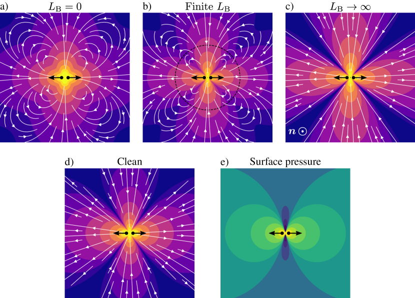
Figure 8: The interfacial velocity and surface pressure fields associated with the $\boldsymbol{\mathsfbi{S}}^{\shortparallel}$ mode are shown for the case of an extensile force dipole. The panels are analogous to those shown in figure 7. The arrows indicate the orientation of the force dipole. Panels (a), (b), and (c) represent one of three leading-order flow modes induced by self-propelled (force- and torque-free) colloids for small-, moderate-, and large-$\mathinner{Bq}$, respectively.

The second term in 68, the $\boldsymbol{A}$ mode, is unaltered from the expression for $\boldsymbol{u}^{\text{m1}}$ for a clean interface 36. Of the three terms, only this one is sensitive to the viscosity contrast. We refer the reader back to figure 6c for a depiction of the associated velocity field. Marangoni and surface-viscous stresses have no effect on this mode, which fails to induce motion of the interface. Its interpretation regarding colloid asymmetry is therefore the same as discussed in section 4.

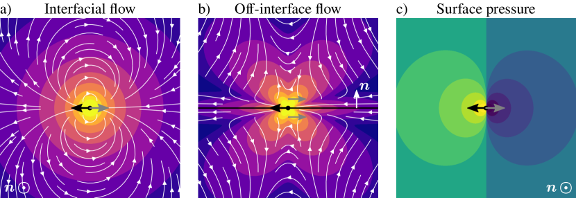
Figure 9: The velocity field $\boldsymbol{B}\boldsymbol{\cdot}\boldsymbol{\mathsfbi{q}}(\boldsymbol{x})$ is visualized for the vector $\boldsymbol{B}$ pointing rightward. This mode is associated with a (viscosity-weighted) pair of force couplets indicated by the arrows. The flow on the interface is shown in (a), and a perpendicular cross-section of the off-interface flow is shown in (b). The associated surface pressure is shown in (c).

The final term of 57, the $\boldsymbol{B}$ mode, has no analogue on a clean interface. Physically, the $\boldsymbol{B}$ mode accounts for the coupling of off-interface forcing of the fluid by the colloid to Marangoni forces that react to enforce interfacial incompressiblity. Interestingly, the coefficient $\boldsymbol{B}$ does not explicitly involve forces on the contact line, in contrast to $\boldsymbol{\mathsfbi{S}}^{\shortparallel}$ and $L_{3}$, but the resulting flow is nonetheless driven by the surface pressure according to 65. The interfacial flow field due to this mode is harmonic, $\nabla_{\mathrm{s}}^{2}\boldsymbol{\mathsfbi{q}}(\boldsymbol{s})=\boldsymbol{0}$ (figure 9a). By 6, it therefore does not induce surface-viscous stresses, explaining why $\boldsymbol{\mathsfbi{q}}$ is independent of $L_{\text{B}}$. Like the $\boldsymbol{\mathsfbi{S}}^{\shortparallel}$ and $L_{3}$ modes, the $\boldsymbol{B}$ mode produces a mirror-symmetric velocity field about the interface. However, while the $\boldsymbol{\mathsfbi{S}}^{\shortparallel}$ and $L_{3}$ modes produce a lamellar velocity field, the velocity field due to the $\boldsymbol{B}$ mode is fully three-dimensional (figure 9b). The surface pressure associated with $\mathsfi q_{i\alpha}(\boldsymbol{x})$ is given by ${\partial\Pi_{\alpha}(\boldsymbol{s},h\hat{\boldsymbol{\imath}}_{3})}/{\partial h}=-s_{\alpha}/2\pi s^{3}$ (figure 9c).

Both the $\boldsymbol{B}$ and $\boldsymbol{A}$ modes can be attributed to the finite protrusion of an adhered colloid from the interface. As the protrusion distance becomes small (or as the geometry of the colloid becomes flat) $\boldsymbol{A}$ and $\boldsymbol{B}$ vanish. It is interesting that finite-size effects enter at dipolar order in this manner. Consider again the velocity profile due to a sphere straddling a clean interface with a $90\text{\,}\mathrm{\SIUnitSymbolDegree}$ contact angle. Here, the size of the sphere matters only at quadrupolar order, through the $a^{2}\nabla^{2}\boldsymbol{\mathsfbi{J}}$ term in 40. In contrast to the $1/r^{3}$ decay of this term, the dipolar $\boldsymbol{A}$ and $\boldsymbol{B}$ modes decay as $1/r^{2}$. On an incompressible (or clean) interface, $\boldsymbol{A}$ vanishes by symmetry for this particular case, but we expect $\boldsymbol{B}\sim a\boldsymbol{F}$, where $\boldsymbol{F}$ is the force driving the colloid. It is intriguing how this finite-protrusion effect arises from interfacial Marangoni forces.

5.3 Discussion

Interfacial incompressibility dramatically restructures the leading-order hydrodynamic modes induced by colloidal particles at interfaces. Marangoni stresses play a major role; even without surface viscosity, only the $L_{3}$ (rotlet) and $\boldsymbol{A}$ modes are unchanged from their counterparts on a clean interface. Marangoni forces also lead to a mode of flow, the $\boldsymbol{B}$ mode given by the final term of 68, that has no analogue on a clean interface.

Recall that, at clean interfaces, the far-field fluid velocity decays at the same rate in directions parallel and normal to the interface: generally, $|\boldsymbol{u}|\sim r^{-1}$ for driven colloids and $|\boldsymbol{u}|\sim r^{-2}$ for active colloids (or colloids driven only by an external torque). If surface-viscous stresses are weak, $\mathinner{Bq}\ll 1$, then this far-field behavior also holds for incompressible interfaces. However, for driven colloids, the leading-order flow normal to the interface is hindered due to the lamellar profile of the force monopole 52. For driven and active colloids alike, the fluid velocity normal to the interface is generally induced to leading order by the dipolar $\boldsymbol{A}$ and $\boldsymbol{B}$ modes (that decay as $1/r^{2}$). The $\boldsymbol{A}$ and $\boldsymbol{B}$ modes therefore have special importance to mass transport enhancement and hydrodynamic interactions normal to the interface. Interestingly, these modes are unaffected by surface viscosity.

However, surface-viscous effects can give rise to very long-ranged flow parallel to the interface. Considering first the spatial behavior along the interfacial plane, we find that, for $\mathinner{Bq}\gg 1$ and distances $s\ll L_{\text{B}}$ from the colloid, $\boldsymbol{u}^{\shortparallel}=\boldsymbol{u}\boldsymbol{\cdot}\boldsymbol{\mathsfbi{I}}_{\mathrm{s}}\sim-\ln s$ for the monopole moment and $\boldsymbol{u}^{\shortparallel}\sim s^{-1}$ for dipole moment. This behavior reflects that of a two-dimensional Stokes flow, which is recovered in the limit of highly viscous interfaces (Saffman & Delbrück, 1975). The slow decay of the velocity field quickens at distances $s\gtrsim L_{\text{B}}$, where bulk-viscous effects inevitably become important. To determine the spatial behavior along the $z$ axis, we observe that the limiting forms of 93 and 96 for $s\ll|z|$ are given by

$$R_{n}(L_{\text{B}};0,|z|) \sim\frac{e^{2|z|/L_{\text{B}}}}{L_{\text{B}}}\operatorname{E}_{1}\!{\left(\frac{2|z|}{L_{\text{B}}}\right)}$$ (71)

$$R^{\prime}_{n}(L_{\text{B}};0,|z|) \sim\frac{e^{2|z|/L_{\text{B}}}}{L_{\text{B}}{\left|z\right|}}\operatorname{E}_{2}\!{\left(\frac{2|z|}{L_{\text{B}}}\right)},$$ (72)

where $\operatorname{E}_{p}(x)=\int_{1}^{\infty}e^{-xt}/t^{p}\mathop{}\!\mathrm{d}t$ is the generalized exponential integral. The asymptotic behavior of this function obeys

$$\operatorname{E}_{p}(x)\sim\begin{cases}[{(-1)}^{p}/(p-1)!]x^{p-1}\ln x&\text{for}\ x\ll 1\\ \operatorname{E}_{p}(x)\sim e^{-x}/x&\text{for}\ x\gg 1\ \text{and for all}\ p,\end{cases}$$ (73)

(Olver et al., 2010) which implies that, for $|z|\ll L_{\text{B}}$, $R_{n}\sim\ln|z|$ and $R^{\prime}_{n}\sim\ln|z|$. Recalling that $R_{n}$ and $R^{\prime}_{n}$ govern the spatial behavior of the monopole and $\boldsymbol{\mathsfbi{S}}^{\shortparallel}$ (dipole) modes, respectively, we see that both are logarithmically divergent in $z$ as $\mathinner{Bq}$ is made large. Therefore, the ‘lamellar’ flows these modes induce persist up to distances $z=O(L_{\text{B}})$ into the surrounding fluid for both driven and active colloids. At distances $z\gg L_{\text{B}}$, we find that $R_{n}\sim|z|^{-1}$ and $R^{\prime}_{n}\sim|z|^{-2}$, recovering the far-field decay expected for $r\gg L_{\text{B}}$. This strong lateral fluid motion has potential implications for mixing generation by colloidal particles at interfaces. For instance, in the presence of a driven or active sheet of interfacially trapped colloids, there may be significant mass transport in directions parallel to the interface via Taylor dispersion. The shear flow driving Taylor dispersion is, in this case, generated by the motion of the colloids rather than motion of a bulk fluid relative to a no-slip boundary. Future work will examine the implications of this fluid motion on transport and mixing rates at interfaces with colloids present.

6 Conclusion

6.1 Summary

We have determined the leading-order far-field flows generated by driven and active colloids trapped at planar fluid interfaces by a pinned contact line for $\mathinner{Ca}\ll 1$. Under these assumptions, the colloid is trapped in a fixed wetting configuration and cannot move perpendicular to the interface. At clean interfaces devoid of surfactant, driven colloids produce “viscosity-averaged” Stokeslets when driven along the interface—the flow is no different than that expected for a colloid driven in an unbounded fluid of viscosity $\bar{\mu}$. Contact-line pinning at small $\mathinner{Ca}$ prevents such colloids from being driven normal to the interface. Similarly, active colloids produce viscosity-averaged force dipoles (stresslets) aligned in the swimming direction, similar to those generated by a swimmer in an unbounded fluid. This stresslet is associated with balanced hydrodynamic thrust and drag in the swimming direction. However, such swimmers also generate additional ‘pumping’ flows that are associated with net hydrodynamic forces and torques on the colloid that are supported by the pinned contact line. These modes vanish if the colloid is adjacent, rather than adhered, to the interface, where it must be force and torque free.

We further consider the effect of surfactants, which render the interface incompressible even in the limit of scant surface concentrations. This constraint is generally applicable to driven and active colloids which move on interfaces for $\mathinner{Ca}\ll 1$. The flow modes associated with forced or self-propelled motion along the interface are altered significantly by interfacial incompressibility. One subset of these modes induce ‘lamellar’ fluid motion for which $u_{z}=0$ at all distances $z$ from the interface. These modes can produce very long ranged flow in the presence of surface-viscous effects. A second subset of modes is responsible for the leading-order fluid motion normal to the interface. These modes occur at dipolar order and are unaffected by surface viscosity.

6.2 Future work and open issues

Future work will probe experimental systems for signatures of the flow modes reported here. For example, the differences we predict for colloids in adhered states versus unadhered states may be useful in distinguishing between these two cases in experiment. Comparison to computational results would also be extremely valuable. Detailed numerical computations of specific types of colloids in different adhered states will yield useful information such as their predicted trajectories and near-field hydrodynamic interactions.

Several open issues remain. We have not considered the effect of contact-line undulations on the flow. Interestingly, interfacial distortion due to such undulations spatially decay at the same rate ($1/r^{2}$) as the flow disturbance due to an active colloid of negligible weight. Thus, these undulations may alter the flows in interesting ways, especially because the contact line of an individual colloid may undulate randomly, being different for every colloid (Stamou et al., 2000; Kaz et al., 2012). Driven and active colloids may also enhance mass transport at interfaces. Enhanced mixing in active colloidal suspensions has been studied extensively in bulk fluids (Darnton et al., 2004; Pushkin & Yeomans, 2013; Lin et al., 2011; Kasyap et al., 2014) and also in the vicinity of solid boundaries (Mathijssen et al., 2015, 2018; Kim & Breuer, 2004). Colloid-induced mixing presents an untapped dimension for interfacial engineering; interfaces are natural sites for many chemical reaction and separation processes. At interfaces, mixing rates will depend on the interfacial rheology and the adhered state of the active colloids that populate the interface. Our work emphasizes the importance of particular far-field flow modes in the generation of mixing by active or passive colloids at interfaces. For an incompressible interface, a subset of these modes promote fluid motion parallel to the interface, which is especially long-ranged for viscous interfaces, and another subset promotes fluid motion normal to the interface. Future work will determine design guidelines for enhancing or directing mass transport at interfaces via colloidal particles by tuning the relative strengths of these modes.

The authors acknowledge useful discussions with Dr. Mehdi Molaei and Ms. Jiayi Deng. This research was made possible by a grant from the Gulf of Mexico Research Initiative. Additional financial support was provided by the National Science Foundation (NSF Grant No. DMR-1607878 and CBET-1943394).

Declaration of Interests. The authors report no conflict of interest.

Appendix A Self-adjoint property of the Green’s functions

To show that the Green’s function $\boldsymbol{\mathsfbi{G}}$ defined by 18 is self-adjoint, i.e., $\boldsymbol{\mathsfbi{G}}(\boldsymbol{x},\boldsymbol{y})=\boldsymbol{\mathsfbi{G}}^{\mathsf{T}}(\boldsymbol{y},\boldsymbol{x})$, we make the following substitutions into 13:

$$\boldsymbol{u}(\boldsymbol{x}) \to\boldsymbol{\mathsfbi{G}}(\boldsymbol{x},\boldsymbol{y})\boldsymbol{\cdot}\boldsymbol{F}, \boldsymbol{u}^{\prime}(\boldsymbol{x}) \to\boldsymbol{\mathsfbi{G}}(\boldsymbol{x},\boldsymbol{y}^{\prime})\boldsymbol{\cdot}\boldsymbol{F}^{\prime},$$ (74)

$$\boldsymbol{\mathsfbi{\sigma}}(\boldsymbol{x}) \to\boldsymbol{\mathsfbi{T}}(\boldsymbol{\mathsfbi{G}};\boldsymbol{x},\boldsymbol{y})\boldsymbol{\cdot}\boldsymbol{F}, \boldsymbol{\mathsfbi{\sigma}}^{\prime}(\boldsymbol{x}) \to\boldsymbol{\mathsfbi{T}}(\boldsymbol{\mathsfbi{G}};\boldsymbol{x},\boldsymbol{y}^{\prime})\boldsymbol{\cdot}\boldsymbol{F}^{\prime},$$

$$\boldsymbol{f}(\boldsymbol{x}) \to-\boldsymbol{F}\delta_{\mathbb{R}^{3}}(\boldsymbol{x}-\boldsymbol{y}), \boldsymbol{f}^{\prime}(\boldsymbol{x}) \to-\boldsymbol{F}\delta_{\mathbb{R}^{3}}(\boldsymbol{x}-\boldsymbol{y}^{\prime}),$$

$$\boldsymbol{f}_{\mathrm{s}}(\boldsymbol{x}) \to-\boldsymbol{F}\delta_{\mathbb{R}^{2}}(\boldsymbol{x}-\boldsymbol{y}), \boldsymbol{f}_{\mathrm{s}}^{\prime}(\boldsymbol{x}) \to-\boldsymbol{F}\delta_{\mathbb{R}^{2}}(\boldsymbol{x}-\boldsymbol{y}^{\prime}).$$

That is, we choose $\boldsymbol{u}$ as the flow field due to a point force $\boldsymbol{F}$ at $\boldsymbol{y}$ and $\boldsymbol{u}^{\prime}$ the flow field due to another point force $\boldsymbol{F}^{\prime}$ at point $\boldsymbol{y}^{\prime}$. The point forces and their locations are arbitrary and may be exerted on either fluid or the interface. Each fluid domain is semi-infinite and bounded only by the interface. With the above substitutions, 13 becomes

$$0=\int_{V^{*}}\left[\delta_{\mathbb{R}^{3}}(\boldsymbol{x}-\boldsymbol{y})\boldsymbol{F}\boldsymbol{\cdot}\boldsymbol{\mathsfbi{G}}(\boldsymbol{x},\boldsymbol{y}^{\prime})\boldsymbol{\cdot}\boldsymbol{F}^{\prime}-\delta_{\mathbb{R}^{3}}(\boldsymbol{x}-\boldsymbol{y}^{\prime})\boldsymbol{F}^{\prime}\boldsymbol{\cdot}\boldsymbol{\mathsfbi{G}}(\boldsymbol{x},\boldsymbol{y})\boldsymbol{\cdot}\boldsymbol{F}\right]\mathop{}\!\mathrm{d}V\\ +\int_{I^{*}}\left[\delta_{\mathbb{R}^{2}}(\boldsymbol{x}-\boldsymbol{y})\boldsymbol{F}\boldsymbol{\cdot}\boldsymbol{\mathsfbi{G}}(\boldsymbol{x},\boldsymbol{y}^{\prime})\boldsymbol{\cdot}\boldsymbol{F}^{\prime}-\delta_{\mathbb{R}^{2}}(\boldsymbol{x}-\boldsymbol{y}^{\prime})\boldsymbol{F}^{\prime}\boldsymbol{\cdot}\boldsymbol{\mathsfbi{G}}(\boldsymbol{x},\boldsymbol{y})\boldsymbol{\cdot}\boldsymbol{F}\right]\mathop{}\!\mathrm{d}A\\ +\oint_{R}\left\{[\boldsymbol{\mathsfbi{T}}(\boldsymbol{x},\boldsymbol{y})\boldsymbol{\cdot}\boldsymbol{F}]\boldsymbol{\cdot}[\boldsymbol{\mathsfbi{G}}(\boldsymbol{x},\boldsymbol{y}^{\prime})\boldsymbol{\cdot}\boldsymbol{F}^{\prime}]-[\boldsymbol{\mathsfbi{T}}(\boldsymbol{x},\boldsymbol{y}^{\prime})\boldsymbol{\cdot}\boldsymbol{F}^{\prime}]\boldsymbol{\cdot}[\boldsymbol{\mathsfbi{G}}(\boldsymbol{x},\boldsymbol{y})\boldsymbol{\cdot}\boldsymbol{F}]\right\}\boldsymbol{\cdot}\hat{\boldsymbol{n}}\mathop{}\!\mathrm{d}S,$$ (75)

where, for brevity, we omit $\boldsymbol{\mathsfbi{G}}$ as an argument to $\boldsymbol{\mathsfbi{T}}$. The integrations in 75 are taken to be over an arbitrary volume that may contain points on the interface. If the boundaries of this volume in each fluid, represented by $R$, are made arbitrarily far from the points $\boldsymbol{y}$ and $\boldsymbol{y}^{\prime}$, then the final integral in 75 vanishes; $\boldsymbol{\mathsfbi{G}}\sim r^{-1}$ and $\boldsymbol{\mathsfbi{T}}(\boldsymbol{\mathsfbi{G}};\!)\sim 1/r^{-2}$, so this integral decays as $L_{V}^{-1}$ as $L_{V}\to\infty$, where $L_{V}$ is the characteristic size of the integration region. Then, using the definition of the Dirac delta, 75 simplifies to

$$\boldsymbol{F}\boldsymbol{\cdot}\boldsymbol{\mathsfbi{G}}(\boldsymbol{y},\boldsymbol{y}^{\prime})\boldsymbol{\cdot}\boldsymbol{F}^{\prime}=\boldsymbol{F}^{\prime}\boldsymbol{\cdot}\boldsymbol{\mathsfbi{G}}(\boldsymbol{y}^{\prime},\boldsymbol{y})\boldsymbol{\cdot}\boldsymbol{F}.$$ (76)

Since $\boldsymbol{F}$, $\boldsymbol{F}^{\prime}$, $\boldsymbol{y}$, and $\boldsymbol{y}^{\prime}$ are all arbitrary, 76 implies that $\boldsymbol{\mathsfbi{G}}(\boldsymbol{y},\boldsymbol{y}^{\prime})=\boldsymbol{\mathsfbi{G}}^{\mathsf{T}}(\boldsymbol{y}^{\prime},\boldsymbol{y})$, that is, $\boldsymbol{\mathsfbi{G}}$ is self-adjoint.

Using the same procedure, it may be shown that $\boldsymbol{\mathsfbi{H}}$ is also self-adjoint. Making a set of substitutions analogous to those appearing in 74 along with the additional substitutions $\boldsymbol{\mathsfbi{\varsigma}}(\boldsymbol{x})\to\boldsymbol{\mathsfbi{\Sigma}}(\boldsymbol{\mathsfbi{H}};\boldsymbol{x},\boldsymbol{y})\boldsymbol{\cdot}\boldsymbol{F}$ and $\boldsymbol{\mathsfbi{\varsigma}}(\boldsymbol{x})\to\boldsymbol{\mathsfbi{\Sigma}}(\boldsymbol{\mathsfbi{H}};\boldsymbol{x},\boldsymbol{y}^{\prime})\boldsymbol{\cdot}\boldsymbol{F}^{\prime}$ into 15, we find

$$0=\boldsymbol{F}^{\prime}\boldsymbol{\cdot}\boldsymbol{\mathsfbi{H}}(\boldsymbol{y}^{\prime},\boldsymbol{y})\boldsymbol{\cdot}\boldsymbol{F}-\boldsymbol{F}\boldsymbol{\cdot}\boldsymbol{\mathsfbi{H}}(\boldsymbol{y},\boldsymbol{y}^{\prime})\boldsymbol{\cdot}\boldsymbol{F}^{\prime}\\ +\oint_{R}\left\{[\boldsymbol{\mathsfbi{T}}(\boldsymbol{x},\boldsymbol{y})\boldsymbol{\cdot}\boldsymbol{F}]\boldsymbol{\cdot}[\boldsymbol{\mathsfbi{H}}(\boldsymbol{x},\boldsymbol{y}^{\prime})\boldsymbol{\cdot}\boldsymbol{F}^{\prime}]-[\boldsymbol{\mathsfbi{T}}(\boldsymbol{x},\boldsymbol{y}^{\prime})\boldsymbol{\cdot}\boldsymbol{F}^{\prime}]\boldsymbol{\cdot}[\boldsymbol{\mathsfbi{H}}(\boldsymbol{x},\boldsymbol{y})\boldsymbol{\cdot}\boldsymbol{F}]\right\}\boldsymbol{\cdot}\hat{\boldsymbol{n}}\mathop{}\!\mathrm{d}S\\ +\oint_{\partial I^{*}}\left\{[\boldsymbol{\mathsfbi{\Sigma}}(\boldsymbol{x},\boldsymbol{y})\boldsymbol{\cdot}\boldsymbol{F}]\boldsymbol{\cdot}[\boldsymbol{\mathsfbi{H}}(\boldsymbol{x},\boldsymbol{y}^{\prime})\boldsymbol{\cdot}\boldsymbol{F}^{\prime}]-[\boldsymbol{\mathsfbi{\Sigma}}(\boldsymbol{x},\boldsymbol{y}^{\prime})\boldsymbol{\cdot}\boldsymbol{F}^{\prime}]\boldsymbol{\cdot}[\boldsymbol{\mathsfbi{H}}(\boldsymbol{x},\boldsymbol{y})\boldsymbol{\cdot}\boldsymbol{F}]\right\}\boldsymbol{\cdot}\hat{\boldsymbol{m}}\mathop{}\!\mathrm{d}C.$$ (77)

In this case, an additional integral over $\partial I^{*}$ appears, which is the curve where our arbitrarily chosen fluid region intersects the interface. Both integrals in 77 vanish as $L_{V}\to\infty$ provided that the Boussinesq length $L_{\text{B}}$ remains finite. For $r\gg L_{\text{B}}$, $\boldsymbol{\mathsfbi{H}}$ and $\boldsymbol{\mathsfbi{G}}$ share the same far-field decay behavior, i.e., $\boldsymbol{\mathsfbi{H}}\sim r^{-1}$. From the remaining two terms in 77, we find $\boldsymbol{\mathsfbi{H}}(\boldsymbol{y},\boldsymbol{y}^{\prime})=\boldsymbol{\mathsfbi{H}}^{\mathsf{T}}(\boldsymbol{y}^{\prime},\boldsymbol{y})$.

Appendix B Derivation of the Green’s functions

Here, we derive the Green’s functions $\boldsymbol{\mathsfbi{G}}$ and $\boldsymbol{\mathsfbi{H}}$ used in sections 4 and 5, respectively. We consider the scenario described in section 3, where two immiscible fluids are separated by a flat interface on the $z=0$ plane, except with no particles present. The velocity field in a region $V^{*}_{\nu}$ that is fully contained in fluid $\nu$ can be represented in boundary integral form as (Kim & Karrila, 1991; Pozrikidis, 1992)

$$\operatorname{\mathbb{I}}_{V^{*}_{\nu}}(\boldsymbol{x})\,\boldsymbol{u}(\boldsymbol{x})=-\frac{1}{\mu_{\nu}}\oint_{\partial V^{*}_{\nu}}{\boldsymbol{\mathsfbi{J}}(\boldsymbol{x},\boldsymbol{y})\boldsymbol{\cdot}[\boldsymbol{\mathsfbi{\sigma}}\boldsymbol{\cdot}\hat{\boldsymbol{n}}](\boldsymbol{y})}\mathop{}\!\mathrm{d}S(\boldsymbol{y})+\oint_{\partial V^{*}_{\nu}}{{[\boldsymbol{u}\hat{\boldsymbol{n}}]}(\boldsymbol{y})\odot\boldsymbol{\mathsfbi{T}}(\boldsymbol{\mathsfbi{J}};\boldsymbol{y},\boldsymbol{x})}\mathop{}\!\mathrm{d}S(\boldsymbol{y})\\ +\frac{1}{\mu_{\nu}}\int_{V^{*}_{\nu}}{\boldsymbol{\mathsfbi{J}}(\boldsymbol{x},\boldsymbol{y})\boldsymbol{\cdot}\boldsymbol{f}(\boldsymbol{y})}\mathop{}\!\mathrm{d}{V(\boldsymbol{y})},$$ (78)

where $\mathsfi J_{ij}(\boldsymbol{x})=(\delta_{ij}/|\boldsymbol{x}|+x_{i}x_{j}/{|\boldsymbol{x}|}^{3})/8\upi$, $\mathsfi T_{ijk}(\boldsymbol{\mathsfbi{J}};\!)=-\delta_{ij}P_{k}(\boldsymbol{\mathsfbi{J}};\!)+(\nabla_{i}\mathsfi J_{jk}-\nabla_{j}\mathsfi J_{ik})$, $\hat{\boldsymbol{n}}$ is the inward-facing unit normal of $\partial V_{\nu}^{*}$, and $\boldsymbol{f}$ is the force density on the fluid. For notational convenience, we hereafter omit $\boldsymbol{\mathsfbi{J}}$ as an argument to $\boldsymbol{\mathsfbi{T}}$.

We choose a point $\boldsymbol{x}=\boldsymbol{y}=h\hat{\boldsymbol{\imath}}_{3}$ at which a point force $\boldsymbol{F}$ is applied. Thus, we set $\boldsymbol{f}(\boldsymbol{y})=\boldsymbol{F}\delta_{\mathbb{R}^{3}}(\boldsymbol{x}-\boldsymbol{y})$. We then apply 78 to a volume $V^{*}_{1}$ in fluid 1 whose boundary $\partial V^{*}_{1}$ is on one side completely adjacent to the interface $I$ and at all other points is made arbitrarily far from the point of forcing $\boldsymbol{y}$. We repeat this process for a similar volume $V^{*}_{2}$ in fluid 2 such that $V^{*}_{\nu}\to V_{\nu}$ and $\partial V^{*}_{1}\cup\partial V^{*}_{2}\to I$. In the resulting pair of equations, only integrations over $I$ make a non-vanishing contribution to $\boldsymbol{u}(\boldsymbol{x})$ in 78. Fourier transformation of these equations gives

$$\operatorname{\mathbb{I}}_{\mathbb{R}_{+}}\!(z)\,\widehat{u}_{i}(\boldsymbol{k},z) =-\widehat{\mathsfi T}_{3\alpha i}(\boldsymbol{\mathsfbi{J}};\boldsymbol{k},z)\widehat{v}_{\alpha}(\boldsymbol{k})-\frac{1}{\mu_{1}}\widehat{\mathsfi J}_{ij}(\boldsymbol{k},z)\widehat{t}^{1}_{j}(\boldsymbol{k})+\frac{\operatorname{\mathbb{I}}_{\mathbb{R}_{+}}\!(h)}{\mu_{1}}\widehat{\mathsfi J}_{ij}(\boldsymbol{k},z-h)F_{j}$$ (79)

$$\operatorname{\mathbb{I}}_{\mathbb{R}_{-}}\!(z)\,\widehat{u}_{i}(\boldsymbol{k},z) =\widehat{\mathsfi T}_{3\alpha i}(\boldsymbol{\mathsfbi{J}};\boldsymbol{k},z)\widehat{v}_{\alpha}(\boldsymbol{k})+\frac{1}{\mu_{2}}\widehat{\mathsfi J}_{ij}(\boldsymbol{k},z)\widehat{t}^{2}_{j}(\boldsymbol{k}),+\frac{\operatorname{\mathbb{I}}_{\mathbb{R}_{-}}\!(h)}{\mu_{2}}\widehat{\mathsfi J}_{ij}(\boldsymbol{k},z-h)F_{j},$$ (80)

where the Fourier transform is defined as $\widehat{\phi}(\boldsymbol{k}):=\iint_{\mathbb{R}^{2}}\phi(\boldsymbol{s})\exp{(-i\boldsymbol{k}\boldsymbol{\cdot}\boldsymbol{s})}\mathop{}\!\mathrm{d}^{2}\boldsymbol{s}$, with $\boldsymbol{s}=x_{1}\hat{\boldsymbol{\imath}}_{1}+x_{2}\hat{\boldsymbol{\imath}}_{2}$ denoting the position vector on the interface. In 79 and 80, $\boldsymbol{t}^{\nu}=\hat{\boldsymbol{\imath}}_{3}\boldsymbol{\cdot}\boldsymbol{\sigma}^{\nu}|_{z=0}$ is the surface traction on the fluid-$\nu$-side of the interface, and $\boldsymbol{v}(\boldsymbol{s})=\boldsymbol{u}(\boldsymbol{s},z=0)$ is the surface velocity on the interface. The Fourier transform of $\boldsymbol{\mathsfbi{J}}$ is given by

$$\widehat{\mathsfi J}_{ij}(\boldsymbol{k},z)=\frac{\delta_{ij}}{2k}e^{-k|z|}+\frac{1}{4k^{3}}\widehat{\nabla}_{i}\widehat{\nabla}_{j}\left[(1+k|z|)e^{-k|z|}\right].$$ (81)

where $\widehat{\nabla}_{i}:=ik_{i}+\delta_{i3}(\partial/\partial z$).

From 3, the Fourier transform of the tangential stress balance on a clean interface is given by

$$\boldsymbol{\mathsfbi{I}}_{\mathrm{s}}\boldsymbol{\cdot}\bigl{(}{[\widehat{\boldsymbol{t}}]}_{I}+\operatorname{\mathbb{I}}_{\{0\}}(h)\,\boldsymbol{F}\bigr{)}=\boldsymbol{0},$$ (82)

and for an incompressible interface from 6 by

$$\boldsymbol{\mathsfbi{I}}_{\mathrm{s}}\boldsymbol{\cdot}\bigl{(}{[\widehat{\boldsymbol{t}}]}_{I}+\operatorname{\mathbb{I}}_{\{0\}}(h)\,\boldsymbol{F}\bigr{)}=i\boldsymbol{k}\widehat{\pi}+\mu_{\mathrm{s}}k^{2}\widehat{\boldsymbol{v}};\quad i\boldsymbol{k}\boldsymbol{\cdot}\boldsymbol{v}=0,$$ (83)

where $k=|\boldsymbol{k}|$.

We multiply 79 by $\mu_{1}$ and take the limit of the resulting equation as $z\to 0^{+}$. Similarly, we multiply 80 by $\mu_{2}$ and take the limit $z\to 0^{-}$. Adding these two results, we find

$$2\bar{\mu}\delta_{i\beta}\widehat{v}_{\beta}(\boldsymbol{k})+\left(\mu_{1}\lim_{z\to 0^{+}}-\mu_{2}\lim_{z\to 0^{-}}\right)\widehat{\mathsfi T}_{3\alpha i}(\boldsymbol{k},z)\widehat{v}_{\alpha}(\boldsymbol{k})+\widehat{\mathsfi J}_{ij}(\boldsymbol{k},0){\left[\widehat{t}_{j}\right]}_{I}(\boldsymbol{k})=\widehat{\mathsfi J}_{ij}(\boldsymbol{k},-h)F_{j},$$ (84)

where $\bar{\mu}=(\mu_{1}+\mu_{2})/2$ is the average viscosity. Using 81 and the definition of $\boldsymbol{\mathsfbi{T}}$, we find that the second term on the left-hand side of 84 reduces to

$$\lim_{z\to 0^{\pm}}\widehat{\mathsfi T}_{3\alpha i}\widehat{v}_{\alpha}=-\left(\pm\frac{\delta_{i\alpha}}{2}+\delta_{i3}\frac{ik_{\alpha}}{2k}\right)\widehat{v}_{\alpha},$$ (85)

which is the Stokes ‘double-layer’ density for either side of the interface. For a clean interface, 82 and 85 in 84 yields, after a trivial Fourier inversion,

$$\bar{\mu}\boldsymbol{v}(\boldsymbol{s})=\boldsymbol{\mathsfbi{I}}_{\mathrm{s}}\boldsymbol{\cdot}\boldsymbol{\mathsfbi{J}}(\boldsymbol{s}-h\hat{\boldsymbol{\imath}}_{3})\boldsymbol{\cdot}\boldsymbol{F},$$ (86)

which shows that the fluid velocity at the interface is independent of the viscosity contrast and simply corresponds to the projection of $\boldsymbol{\mathsfbi{J}}$, shifted to $z=h$, onto the interface at $z=0$.

We may do the same for an incompressible interface by instead using 83 in 84, from which we obtain

$$\left(\bar{\mu}+\frac{1}{2}\mu_{\mathrm{s}}k\right)\widehat{v}_{\alpha}+\frac{ik_{\alpha}}{4k}\widehat{\pi}=\widehat{\mathsfi J}_{\alpha j}|_{z=-h}F_{j}.$$ (87)

Taking the inner product of 87 with $i\boldsymbol{k}$ and solving for $\widehat{\pi}$ yields

$$\widehat{\pi}(\boldsymbol{k}) =-\frac{4}{k}i\boldsymbol{k}\boldsymbol{\cdot}\widehat{\mathsfbi J}(\boldsymbol{k},-h)\boldsymbol{\cdot}\boldsymbol{F}$$ (88)

$$=\frac{e^{-k|h|}}{k^{2}}\left[(k|h|-1)i\boldsymbol{k}+k^{2}h\boldsymbol{i}_{z}\right]\boldsymbol{\cdot}\boldsymbol{F}.$$

Letting $\pi(\boldsymbol{s},h)=\boldsymbol{\Pi}(\boldsymbol{s},h)\boldsymbol{\cdot}\boldsymbol{F}$ and carrying out the Fourier inversion to real space, we obtain

$$\boldsymbol{\Pi}(\boldsymbol{s},h)=|h|\left(\boldsymbol{\nabla}_{\!\mathrm{s}}-\hat{\boldsymbol{\imath}}_{3}\frac{\partial}{\partial h}\right)\frac{1}{4\upi\sqrt{s^{2}+h^{2}}}+\frac{\boldsymbol{s}}{4\upi s^{2}}\left(1-\frac{|h|}{\sqrt{s^{2}+h^{2}}}\right),$$ (89)

which reduces to equation 46 of the main text.

Noting that $\boldsymbol{v}(\boldsymbol{s})\equiv\boldsymbol{\mathsfbi{H}}(\boldsymbol{x},\boldsymbol{y})|_{z=0}\boldsymbol{\cdot}\boldsymbol{F}$, we combine 88 and 87 and solve for $\widehat{\boldsymbol{v}}$ to give

$$\widehat{\mathsfbi H}(\boldsymbol{k},z=0,h) =\frac{2}{2\bar{\mu}+\mu_{\mathrm{s}}k}\left(\boldsymbol{\mathsfbi{I}}_{\mathrm{s}}-\frac{\boldsymbol{kk}}{k^{2}}\right)\boldsymbol{\cdot}\widehat{\mathsfbi J}(\boldsymbol{k},-h)$$ (90)

$$=\frac{e^{-k|h|}}{2\bar{\mu}+\mu_{\mathrm{s}}k}\left(\frac{\boldsymbol{\mathsfbi{I}}_{\mathrm{s}}}{k}-\frac{\boldsymbol{kk}}{k^{3}}\right).$$

Surface incompressibility of $\boldsymbol{\mathsfbi{H}}$ is easily verified by contracting the right-hand side of 90 with $i\boldsymbol{k}$, thereby taking the divergence in Fourier space, which vanishes. We also see from 90 that a force perpendicular to the interface generates no interfacial flow; $\mathsfi H_{i3}(\boldsymbol{x}\in I,h)=0$. We conclude that the flow due to the $z$-component of the force is the same as that for a rigid, no-slip wall, as is also noted by Bławzdziewicz et al. (1999).

The self-adjoint property of $\boldsymbol{\mathsfbi{H}}$ 42 permits us to swap the roles of $h$ and $z$ in 90;

$$\widehat{\mathsfbi H}(\boldsymbol{k},z,h=0):=\widehat{\mathsfbi H}^{0}(\boldsymbol{k},z)=\frac{e^{-k|z|}}{2\bar{\mu}+\mu_{\mathrm{s}}k}\left(\frac{\boldsymbol{\mathsfbi{I}}_{\mathrm{s}}}{k}-\frac{\boldsymbol{kk}}{k^{3}}\right).$$ (91)

From the interfacial flow profile due to a point force at $z=h$ 90, we automatically obtain the flow at all points $\boldsymbol{x}$ due to a point force at the interface ($h=0$). Fourier inversion of 91 to real space gives

$$\mathsfi H^{0}_{\alpha\beta}(L_{\text{B}};\boldsymbol{s},z)=\frac{1}{4\upi\bar{\mu}}R_{0}(L_{\text{B}};s,|z|)\delta_{\alpha\beta}+\frac{1}{2\upi\bar{\mu}}R_{2}(L_{\text{B}};s,|z|)\left\{\hat{s}_{\alpha}\hat{s}_{\beta}\right\}_{0},$$ (92)

where $L_{\text{B}}=\mu_{\mathrm{s}}/\bar{\mu}$ and $s=|\boldsymbol{s}|$. Equation 92 is the same as 43 of the main text. The functions $R_{n}$ are given by

$$R_{n}(L_{\text{B}};s,\zeta)=\int_{0}^{\infty}\frac{e^{-k\zeta}}{2+L_{\text{B}}k}J_{n}(ks)\mathop{}\!\mathrm{d}k,$$ (93)

where $J_{n}$ is the Bessel function of the first kind of order $n$. For $L_{\text{B}}=0$, $R_{n}$ reduces to

$$R_{n}(0;s,|z|)=\frac{(r-|z|)^{n}}{2rs^{n}},$$ (94)

where $r=\sqrt{s^{2}+z^{2}}$. To obtain (surface) gradients of 92, we may take the tensor product of 91 with $i\boldsymbol{k}$ and repeat the Fourier inversion process to give

$$\frac{\partial\mathsfi H^{0}_{\alpha\beta}}{\partial s_{\gamma}}=-\frac{R_{1}^{\prime}(L_{\text{B}};s,|z|)}{8\upi\bar{\mu}}\left(\hat{s}_{\alpha}\delta_{\beta\gamma}+\hat{s}_{\beta}\delta_{\gamma\alpha}-3\hat{s}_{\gamma}\delta_{\alpha\beta}\right)+\frac{R_{3}^{\prime}(L_{\text{B}};s,|z|)}{2\upi\bar{\mu}}\left\{\hat{s}_{\alpha}\hat{s}_{\beta}\hat{s}_{\gamma}\right\}_{0},$$ (95)

where

$$R^{\prime}_{n}(L_{\text{B}};s,\zeta)=\frac{\partial R_{n}}{\partial\zeta}=-\int_{0}^{\infty}\frac{ke^{-k\zeta}}{2+L_{\text{B}}k}J_{n}(ks)\mathop{}\!\mathrm{d}k.$$ (96)

For $L_{\text{B}}=0$, $R^{\prime}_{n}$ reduces to

$$R_{n}^{\prime}(0;s,|z|)=-\frac{s^{n}(nr+|z|)}{2r^{3}(r+|z|)^{n}}.$$ (97)

To determine the flow for all $\boldsymbol{x}$ and $\boldsymbol{y}$, we can sum 79 and 80 to eliminate the Stokes double layer, which gives

$$\widehat{u}_{i}(\boldsymbol{k},z;h)=-\frac{1}{\bar{\mu}}\widehat{\mathsfi J}_{ij}(\boldsymbol{k},z)\widehat{q}_{j}(\boldsymbol{k};h)+\frac{1}{\mu(h)}\widehat{\mathsfi J}_{ij}(\boldsymbol{k},z-h)F_{j}$$ (98)

where

$$\widehat{\boldsymbol{q}}(\boldsymbol{k};h)=\bar{\mu}{\left(\frac{\widehat{\boldsymbol{t}^{1}}(\boldsymbol{k})}{\mu_{1}}-\frac{\widehat{\boldsymbol{t}^{2}}(\boldsymbol{k})}{\mu_{2}}\right)}$$

is the Stokes single-layer density in Fourier space. For a clean interface, setting $z=0$ in 98 and putting 86 into the result yields

$$\widehat{\boldsymbol{q}}(k;h)=4k{\left(\boldsymbol{\mathsfbi{I}}-\frac{\mu(h)}{\bar{\mu}}\boldsymbol{\mathsfbi{I}}_{\mathrm{s}}\right)}\boldsymbol{\cdot}\widehat{\mathsfbi J}(\boldsymbol{k},-h)\boldsymbol{\cdot}\boldsymbol{F}.$$ (99)

After inserting 99 back into 98, lengthy algebraic manipulation and inversion of $\widehat{\boldsymbol{u}}$ to real space yields the velocity field in terms of the hydrodynamic image system 18, with $\boldsymbol{u}\equiv\boldsymbol{\mathsfbi{G}}\boldsymbol{\cdot}\boldsymbol{F}$. A similar procedure may be used to fully determine $\boldsymbol{\mathsfbi{H}}(\boldsymbol{x},\boldsymbol{y})$, but we do not require that result in this article. See also Bławzdziewicz et al. (1999) and Fischer et al. (2006) for computations of $\boldsymbol{\mathsfbi{H}}$ via different approaches.

References

- Aderogba & Blake (1978) Aderogba, K. & Blake, J. R. 1978 Action of a force near the planar surface between two semi-infinite immiscible liquids at very low Reynolds numbers. Bulletin of the Australian Mathematical Society 18 (3), 345–356.
- Ahmadzadegan et al. (2019) Ahmadzadegan, Adib, Wang, Shiyan, Vlachos, Pavlos P. & Ardekani, Arezoo M. 2019 Hydrodynamic attraction of bacteria to gas and liquid interfaces. Physical Review E 100 (6), 062605.
- Bławzdziewicz et al. (1999) Bławzdziewicz, Jerzy, Cristini, Vittorio & Loewenberg, Michael 1999 Stokes flow in the presence of a planar interface covered with incompressible surfactant. Physics of Fluids 11 (2), 251–258.
- Boniello et al. (2015) Boniello, Giuseppe, Blanc, Christophe, Fedorenko, Denys, Medfai, Mayssa, Mbarek, Nadia Ben, In, Martin, Gross, Michel, Stocco, Antonio & Nobili, Maurizio 2015 Brownian diffusion of a partially wetted colloid. Nature Materials 14 (9), 908–911, number: 9 Publisher: Nature Publishing Group.
- Colosqui et al. (2013) Colosqui, Carlos E., Morris, Jeffrey F. & Koplik, Joel 2013 Colloidal adsorption at fluid interfaces: Regime crossover from fast relaxation to physical aging. Physical Review Letters 111 (2), 028302.
- Dani et al. (2015) Dani, Archit, Keiser, Geoff, Yeganeh, Mohsen & Maldarelli, Charles 2015 Hydrodynamics of particles at an oil–water interface. Langmuir 31 (49), 13290–13302.
- Darnton et al. (2004) Darnton, Nicholas, Turner, Linda, Breuer, Kenneth & Berg, Howard C. 2004 Moving Fluid with Bacterial Carpets. Biophysical Journal 86 (3), 1863–1870.
- Deng et al. (2020) Deng, Jiayi, Molaei, Mehdi, Chisholm, Nicholas G. & Stebe, Kathleen J. 2020 Motile Bacteria at Oil–Water Interfaces: Pseudomonas aeruginosa. Langmuir 36 (25), 6888–6902, publisher: American Chemical Society.
- Desai et al. (2018) Desai, Nikhil, Shaik, Vaseem A. & Ardekani, Arezoo M. 2018 Hydrodynamics-mediated trapping of micro-swimmers near drops. Soft Matter 14 (2), 264–278.
- Di Leonardo et al. (2011) Di Leonardo, R., Dell’Arciprete, D., Angelani, L. & Iebba, V. 2011 Swimming with an image. Physical Review Letters 106 (3), 038101.
- Dörr & Hardt (2015) Dörr, Aaron & Hardt, Steffen 2015 Driven particles at fluid interfaces acting as capillary dipoles. Journal of Fluid Mechanics 770, 5–26, publisher: Cambridge University Press.
- Dörr et al. (2016) Dörr, Aaron, Hardt, Steffen, Masoud, Hassan & Stone, Howard A. 2016 Drag and diffusion coefficients of a spherical particle attached to a fluid–fluid interface. Journal of Fluid Mechanics 790, 607–618.
- Elfring et al. (2016) Elfring, Gwynn J., Leal, L. Gary & Squires, Todd M. 2016 Surface viscosity and Marangoni stresses at surfactant laden interfaces. Journal of Fluid Mechanics 792, 712–739.
- Fischer (2004) Fischer, Th. M. 2004 The drag on needles moving in a Langmuir monolayer. Journal of Fluid Mechanics 498, 123–137.
- Fischer et al. (2006) Fischer, Th. M., Dhar, P. & Heinig, P. 2006 The viscous drag of spheres and filaments moving in membranes or monolayers. Journal of Fluid Mechanics 558, 451.
- Giacché et al. (2010) Giacché, Davide, Ishikawa, Takuji & Yamaguchi, Takami 2010 Hydrodynamic entrapment of bacteria swimming near a solid surface. Physical Review E 82 (5), 056309.
- Hughes et al. (1981) Hughes, B. D., Pailthorpe, B. A. & White, L. R. 1981 The translational and rotational drag on a cylinder moving in a membrane. Journal of Fluid Mechanics 110, 349–372, publisher: Cambridge University Press.
- Kasyap et al. (2014) Kasyap, T. V., Koch, Donald L. & Wu, Mingming 2014 Hydrodynamic tracer diffusion in suspensions of swimming bacteria. Physics of Fluids 26 (8), 081901.
- Kaz et al. (2012) Kaz, David M., McGorty, Ryan, Mani, Madhav, Brenner, Michael P. & Manoharan, Vinothan N. 2012 Physical ageing of the contact line on colloidal particles at liquid interfaces. Nature Materials 11 (2), 138–142.
- Kim & Breuer (2004) Kim, Min Jun & Breuer, Kenneth S. 2004 Enhanced diffusion due to motile bacteria. Physics of Fluids 16 (9), L78–L81.
- Kim & Karrila (1991) Kim, Sangtae & Karrila, Seppo J. 1991 Microhydrodynamics: principles and selected applications. Butterworth-Heinemann.
- Lauga et al. (2006) Lauga, Eric, DiLuzio, Willow R., Whitesides, George M. & Stone, Howard A. 2006 Swimming in Circles: Motion of Bacteria near Solid Boundaries. Biophysical Journal 90 (2), 400–412.
- Lauga & Powers (2009) Lauga, Eric & Powers, Thomas R. 2009 The hydrodynamics of swimming microorganisms. Reports on Progress in Physics 72 (9), 096601.
- Levine & MacKintosh (2002) Levine, Alex J. & MacKintosh, F. C. 2002 Dynamics of viscoelastic membranes. Physical Review E 66 (6), 061606.
- Lin et al. (2011) Lin, Zhi, Thiffeault, Jean-Luc & Childress, Stephen 2011 Stirring by squirmers. Journal of Fluid Mechanics 669, 167–177.
- Lopez & Lauga (2014) Lopez, Diego & Lauga, Eric 2014 Dynamics of swimming bacteria at complex interfaces. Physics of Fluids 26 (7), 071902.
- Malgaretti et al. (2016) Malgaretti, P., Popescu, M. N. & Dietrich, S. 2016 Active colloids at fluid interfaces. Soft Matter 12 (17), 4007–4023.
- Mathijssen et al. (2018) Mathijssen, Arnold J. T. M., Guzmán-Lastra, Francisca, Kaiser, Andreas & Löwen, Hartmut 2018 Nutrient Transport Driven by Microbial Active Carpets. Physical Review Letters 121 (24), 248101.
- Mathijssen et al. (2015) Mathijssen, A. J. T. M., Pushkin, D. O. & Yeomans, J. M. 2015 Tracer trajectories and displacement due to a micro-swimmer near a surface. Journal of Fluid Mechanics 773 (2015), 498–519.
- Olver et al. (2010) Olver, Frank W. J., Lozier, Daniel W., Boisvert, Ronald F. & Clark, Charles W., ed. 2010 NIST handbook of mathematical functions. Cambridge ; New York: Cambridge University Press : NIST, oCLC: ocn502037224.
- Pimponi et al. (2016) Pimponi, D., Chinappi, M., Gualtieri, P. & Casciola, C. M. 2016 Hydrodynamics of flagellated microswimmers near free-slip interfaces. Journal of Fluid Mechanics 789, 514–533.
- Pozrikidis (1992) Pozrikidis, C. 1992 Boundary Integral and Singularity Methods for Linearized Viscous Flow, 1st edn. Cambridge University Press.
- Pozrikidis (2007) Pozrikidis, C. 2007 Particle motion near and inside an interface. Journal of Fluid Mechanics 575, 333–357.
- Pushkin & Yeomans (2013) Pushkin, Dmitri O. & Yeomans, Julia M. 2013 Fluid Mixing by Curved Trajectories of Microswimmers. Physical Review Letters 111 (18), 188101.
- Ranger (1978) Ranger, K. B. 1978 The circular disk straddling the interface of a two-phase flow. International Journal of Multiphase Flow 4 (3), 263–277.
- Saffman & Delbrück (1975) Saffman, P. G. & Delbrück, M. 1975 Brownian motion in biological membranes. Proceedings of the National Academy of Sciences 72 (8), 3111–3113.
- Shaik & Ardekani (2017) Shaik, Vaseem A. & Ardekani, Arezoo M. 2017 Motion of a model swimmer near a weakly deforming interface. Journal of Fluid Mechanics 824, 42–73.
- Sickert et al. (2007) Sickert, M., Rondelez, F. & Stone, H. A. 2007 Single-particle Brownian dynamics for characterizing the rheology of fluid Langmuir monolayers. Europhysics Letters (EPL) 79 (6), 66005.
- Spagnolie & Lauga (2012) Spagnolie, Saverio E. & Lauga, Eric 2012 Hydrodynamics of self-propulsion near a boundary: predictions and accuracy of far-field approximations. Journal of Fluid Mechanics 700, 105–147.
- Stamou et al. (2000) Stamou, Dimitris, Duschl, Claus & Johannsmann, Diethelm 2000 Long-range attraction between colloidal spheres at the air-water interface: The consequence of an irregular meniscus. Physical Review E 62 (4), 5263–5272, publisher: American Physical Society.
- Stone & Ajdari (1998) Stone, Howard A. & Ajdari, Armand 1998 Hydrodynamics of particles embedded in a flat surfactant layer overlying a subphase of finite depth. Journal of Fluid Mechanics 369, 151–173, publisher: Cambridge University Press.
- Stone & Masoud (2015) Stone, Howard A. & Masoud, Hassan 2015 Mobility of membrane-trapped particles. Journal of Fluid Mechanics 781, 494–505.
- Vaccari et al. (2018) Vaccari, Liana, Molaei, Mehdi, L. Leheny, Robert & J. Stebe, Kathleen 2018 Cargo carrying bacteria at interfaces. Soft Matter 14 (27), 5643–5653.
- Wang et al. (2017) Wang, Xiaolu, In, Martin, Blanc, Christophe, Würger, Alois, Nobili, Maurizio & Stocco, Antonio 2017 Janus Colloids Actively Rotating on the Surface of Water. Langmuir 33 (48), 13766–13773.