PLATON II: New Capabilities and a Comprehensive Retrieval on HD 189733b Transit and Eclipse Data

Abstract

Recently, we introduced PLanetary Atmospheric Tool for Observer Noobs (PLATON), a Python package that calculates model transmission spectra for exoplanets and retrieves atmospheric characteristics based on observed spectra. We now expand its capabilities to include the ability to compute secondary eclipse depths. We have also added the option to calculate models using the correlated-$k$ method for radiative transfer, which improves accuracy without sacrificing speed. Additionally, we update the opacities in PLATON–many of which were generated using old or proprietary line lists–using the most recent and complete public line lists. These opacities are made available at R=1000 and R=10,000 over the $0.3-30$ µm range, and at R=375,000 in select near IR bands, making it possible to utilize PLATON for ground-based high resolution cross correlation studies. To demonstrate PLATON’s new capabilities, we perform a retrieval on published HST and Spitzer transmission and emission spectra of the archetypal hot Jupiter HD 189733b. This is the first joint transit and secondary eclipse retrieval for this planet in the literature, as well as the most comprehensive set of both transit and eclipse data assembled for a retrieval to date. We find that these high signal-to-noise data are well-matched by atmosphere models with a C/O ratio of $0.66_{-0.09}^{+0.05}$ and a metallicity of $12_{-5}^{+8}$ times solar where the terminator is dominated by extended nanometer-sized haze particles at optical wavelengths. These are among the smallest uncertainties reported to date for an exoplanet, demonstrating both the power and the limitations of HST and Spitzer exoplanet observations.

1. Introduction

The emission spectra of exoplanets provide unique insights into their atmospheric properties (e.g., Madhusudhan, 2018). By measuring the difference between the in-eclipse and out-of-eclipse flux when the planet passes behind the star (‘secondary eclipse’), one can measure the flux emitted by the planet as a function of wavelength. Secondary eclipse observations probe the compositions and temperature-pressure profiles of their dayside atmospheres. This technique was used to derive the first atmospheric composition measurement for a Neptune-mass planet (GJ 436b; Stevenson et al. 2010), the first definitive detection of a thermal inversion in the atmosphere of an ultra-hot Jupiter (Haynes et al., 2015), and dayside water abundance measurements for several hot Jupiters (e.g. Kreidberg et al. 2014; Line et al. 2016; Pinhas et al. 2019). Emission spectroscopy at high spectral resolution ($R>20,000$) has led to the detection of CO, H₂O, and HCN in exoplanet atmospheres (i.e. Snellen et al. 2010; Birkby 2018), including in non-transiting planets like 51 Pegasi b (Brogi et al., 2013). By measuring the atmospheric compositions of these planets, we can obtain new insights into present-day atmospheric processes such as disequilibrium chemistry (e.g., Moses et al. 2013), as well as their past formation and migration histories (e.g., Öberg et al. 2011; Madhusudhan et al. 2014; Ali-Dib 2017; Cridland et al. 2019; Booth & Ilee 2019).

Ideally, we would extract atmospheric parameters from observed emission spectra using a Bayesian retrieval code. However, there is an overall lack of open source retrieval codes that can handle emission spectra. A similar lack of retrieval codes for transit spectra motivated us to write PLATON (Zhang et al., 2019), a fast, open source, easy to use, and easy to understand forward modeling and retrieval code that traces its lineage back to Exo-Transmit (Kempton et al., 2017). PLATON has since been used in several papers: a few exploring the atmospheric properties of observed planets (Chachan et al., 2019; Kirk et al., 2019; Guo et al., 2020), and one demonstrating the possibility of using K-means clustering to speed up retrievals by 40% (Hayes et al., 2020). In the latter study, the speed of PLATON was especially useful due to the necessity of running many retrievals. We now expand PLATON’s capabilities to include thermal emission and compare the resulting models and atmospheric retrievals to that of another retrieval code in order to validate this new functionality.

We utilize the open source TauREx code (Waldmann et al., 2015; Al-Refaie et al., 2019), which has been used in multiple published studies (i.e. Komacek et al. 2019; Shulyak et al. 2019), for this comparison. Specially, we compare to TauREx 3, the latest release. PLATON and TauREx were developed independently of each other, and there are several key differences between their functionalities. TauREx is a sophisticated code which supports free retrieval of chemical abundances in addition to equilibrium chemistry retrievals. PLATON only allows for retrievals using equilibrium chemistry, with atmospheric metallicity and C/O ratio as free parameters. When calculating this equilibrium chemistry, PLATON uses GGchem, which can account for losses due to condensation (Woitke et al., 2018), whereas TauREx assumes that everything stays in the gas phase. PLATON also uses opacities generated from the latest line lists for water (Polyansky et al., 2018), methane (Rey et al., 2017), and ammonia (Coles et al., 2019), which are significantly more complete and accurate than the line lists that were available at the time TauREx was released.

The two codes also differ in their treatment of aerosols. Both support Rayleigh scattering, although PLATON also supports Rayleigh-like scattering by allowing for a variable scattering strength and slope ($\sigma(\lambda)=A\sigma_{\rm Rayleigh}(\lambda)(1\mu m/\lambda)^{s}$). Both also support Mie scattering, but with different parameterizations. TauREx has three ways of approximating Mie opacity: a gray opacity, the parameterization of Lee et al. (2013) ($Q_{ext}=\frac{5}{Q_{0}x^{-4}+x^{0}.2}$), and an analytical calculation of the Mie opacity of spherical particles with a size distribution given by Equation 36 or Equation 37 of Sharp & Burrows (2007). PLATON analytically calculates the Mie opacity of spherical particles with a lognormal size distribution, as explained in Zhang et al. (2019). In this study we explore the impact of these differences on our models using the benchmark hot Jupiter HD 189733b (Bouchy et al., 2005) as our test case.

Aside from TauREx, other open source retrieval codes include the recently released Helios-r2 (Kitzmann et al., 2020) and the Bayesian Atmospheric Radiative Transfer (BART) code (Blecic, 2016; Blecic et al., 2017). Helios-r2 is primarily intended for brown dwarfs and supports both free retrievals and gas-only equilibrium retrievals without clouds. It does not use a parameterized T/P profile, but retrieves the temperatures of individual layers in the atmosphere, with constraints on how much the temperature can vary from layer to layer. This approach is suitable for the high signal-to-noise regime of brown dwarfs, but not ideal for exoplanets.

BART is partially described in one subsection of a dissertation (Blecic, 2016) and one subsection of a paper (Blecic et al., 2017), but has not been described in detail in a peer reviewed paper. BART uses a custom MCMC code, MC³, to perform retrievals using either free abundances or gas-only equilibrium chemistry, the latter of which is computed by TEA (Blecic et al., 2016). It supports two T/P profile parameterizations: Madhusudhan & Seager (2009) and Guillot (2010). However, BART does not provide opacity data, and the opacity calculator it provides does not support ExoMol line lists. In addition, TEA is slow, taking 2-3 s of CPU time per temperature/pressure point, and has convergence problems below 400 K (Woitke et al., 2018).

Last in our roundup of retrieval codes is petitRADTRANS, a forward modelling code that does not support retrievals, but is fast enough to be wrapped in a Bayesian retrieval framework (Mollière et al., 2019). Mollière et al. (2019) benchmark against PLATON and find that although PLATON is much faster overall, the two codes are comparable in speed for the same number of wavelength points. petitRADTRANS only supports free abundances, and uses either correlated-k (R=1000) or line-by-line (R=$10^{6}$) radiative transfer, with a T/P profile parameterization that is a variant of Guillot (2010). To our knowledge, PLATON is unique among open source retrieval codes in supporting equilibrium condensation in a Bayesian retrieval framework, and our opacities are based on the most up-to-date line lists.

We utilize PLATON to carry out the first joint retrieval on published emission and transmission spectroscopy for HD 189733b, resulting in improved constraints on its atmospheric composition. PLATON is also capable of calculating transit and eclipse spectra at R=375,000, and we compare our model to published high-resolution ($R\sim 100,000$) CRIRES emission spectroscopy for this planet to search for previously reported signatures of H₂O and HCN (de Kok et al., 2013; Birkby et al., 2013; Brogi et al., 2016; Cabot et al., 2019) in addition to an unreported molecule: CH₄.

In Section 2, we describe the emission spectrum and secondary eclipse depth calculator. Section 3 describes the opacity update, while Section 4 describes other new features and improvements in PLATON, including the new correlated-$k$ capability and optional model parameters, including a chemical quench pressure and a HST/WFC3 offset. In Section 5, we perform a joint retrieval of the transit and eclipse spectra of HD 189733b to infer its atmospheric properties and confirm published high-resolution detections of H₂O while calling into question the reported high-resolution detection of HCN. We summarize our conclusions in Section 6.

2. Emission Spectrum and Secondary Eclipse depth calculator

2.1. Algorithm

Our emission spectrum and secondary eclipse depth calculator utilizes much of the same code as the transit depth calculator presented in our first paper (Zhang et al., 2019). Given a planetary mass, radius, metallicity, C/O ratio, and temperature-pressure profile, we compute equilibrium molecular abundances for 250 pressures uniformly distributed in log(P). We then solve the hydrostatic equation to determine the height corresponding to each pressure. With molecular abundances, temperatures, and pressures as a function of height, the emergent flux is given by:

$$F_{p\lambda}=2\pi\int_{0}^{\infty}\int_{0}^{1}B_{\lambda}(\tau_{\lambda})e^{-\tau_{\lambda}/\mu}d\mu d\tau_{\lambda}$$ (1)

where $B_{\lambda}(\tau_{\lambda})$ is the Planck function at an optical depth of $\tau_{\lambda}$, and $\mu$ is the cosine of the viewing angle with respect to the vertical. Here, we are making the assumption that the source function is the Planck function, which in turn requires that scattering contributes negligibly to the emission. Adding scattering as an emission source would make the problem much more complex because it would be non-local: the source function at a certain location would depend on scattered photons from other locations.

Directly integrating Equation 1 would require evaluating the integrand hundreds of millions of times–once for every combination of wavelength, $\tau_{\lambda}$, and $\mu$. We instead rewrite the double integral as a single integral with a special function:

$$F_{p\lambda}=2\pi\int_{0}^{\infty}B_{\lambda}(\tau_{\lambda})E_{2}(\tau_{\lambda})d\tau_{\lambda}$$ (2)

where $E_{2}$ is the exponential integral, defined as:

$$E_{2}(x)=\int_{1}^{\infty}\frac{e^{-xt}}{t^{2}}dt$$ (3)

We discretize and reformulate the equation as follows:

$$F_{p\lambda} \approx 2\pi\sum_{0}^{N}B(\tau_{\lambda,i})E_{2}(\tau_{\lambda,i})\Delta\tau_{\lambda,i}$$ (4)

$$\approx 2\pi\sum_{0}^{N-1}-B(\tau_{\lambda,i})(E_{3}(\tau_{\lambda,i+1})-E_{3}(\tau_{\lambda,i})),$$ (5)

where the second equation follows from the first because the integral of $E_{2}(x)$ is $-E_{3}(x)+C$. Reformulating the equation in this way has the virtue of guaranteeing that the result is exactly correct for an isothermal atmosphere. For an isothermal atmosphere, B is constant; therefore, for every layer i except the two boundaries, the $E_{3}(\tau_{i+1})$ term is cancelled by the $-E_{3}(\tau_{i})$ term in layer i+1. The numerical integration therefore gives $2\pi B(E_{3}(\tau_{\lambda,0})-E_{3}(\tau_{\lambda,N}))$. Assuming the top of the atmosphere has an optical depth of 0 and the bottom has an optical depth of infinity, we obtain $F=\pi B$–exactly the correct result for an isothermal atmosphere. In practice, we find that this trick reduces the error for non-isothermal atmospheres as well, especially when the temperature gradient is small. This method of replacing $g(x)\Delta x$ with $G(x_{2})-G(x_{1})$ (where g(x) is the derivative of G(x)) before integrating was inspired by the TauREx source code, which uses the same technique in combination with Gaussian quadrature.

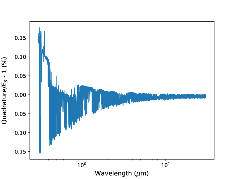
The $E_{3}$ exponential integral is a special function defined by scipy, eliminating the need to perform integrals to evaluate it. It is also continuous, infinitely differentiable, and approaches 0.5 as $x\to 0$ and 0 as $x\to\infty$. These properties mean that $E_{3}$ poses no problems for numerical integration. To further speed up the code, we evaluate $E_{3}(x)$ on a logarithmic grid spanning $x=10^{-6}$ to $x=10^{2}$ during initialization of the eclipse depth calculator, and interpolate from this grid thereafter. The interpolation is accurate to $1.2\times 10^{-5}$, and is therefore a negligible source of error. The more common approach to integrating Equation 1, adopted by TauREx and HELIOS-r2, is to use Gaussian quadrature. Compared to our approach, Gaussian quadrature is 4 times slower and introduces errors of $\sim$0.2% for the test planet in Subsection 2.4 when 4 points are used (Figure 1). This error is utterly negligible compared to the other sources of error we explore in Subsection 2.4.

Figure 1.— Fractional error introduced by using Gaussian quadrature with 4 points instead of $E_{3}$, for the test planet in Subsection 2.4.

To derive a monochromatic eclipse depth from the emergent flux, we multiply by the square of the planet-to-star radius ratio and divide by the stellar emergent flux:

$$D_{\lambda}=\bigg{(}\frac{R_{p\lambda}}{R_{s}}\bigg{)}^{2}\frac{F_{p\lambda}}{F_{s\lambda}}$$ (7)

The stellar spectrum is calculated by interpolating the BT-Settl (AGSS2009) stellar spectral grid (Allard et al., 2012), as provided by the Spanish Virtual Observatory. Here, the wavelength-dependent planet radius $R_{p\lambda}$ is defined as the radius at which the radial optical depth reaches one, assuming that the limb has the same temperature-pressure profile as the dayside. (This is not to be confused with the white light planet radius the users pass into PLATON, which is the radius at a pressure of 1 bar.) This approach differs from those of previous studies (i.e. Waldmann et al. 2015), which typically fix the radius to the value measured from the optical or near-infrared transit depth. This is larger than the effective planet size for emission spectroscopy, as starlight transmitted through the planet’s limb should reach an optical depth of one at lower pressures than for direct emission. Our approach, although an improvement, is still only an approximation. The planetary limb is usually colder than the day side, and even if it were not, Equation 7 is only strictly true if the atmospheric scale height is a negligible fraction of the planetary radius. These inaccuracies are expected to cause errors on the order of 1% for hot Jupiters, since the scale height of a hot Jupiter is of order 1% of the radius. For further discussion of the difficulty in choosing a photospheric radius and the error this introduces, we refer the reader to Fortney et al. (2019).

When fitting observational data, we typically want band-integrated fluxes and secondary eclipse depths. The band-integrated flux is equal to the number of photons emitted from the planet within the band, and the secondary eclipse depth is that value divided by the number of photons emitted from the star within the band. The eclipse depth for the band $\lambda_{1}$–$\lambda_{2}$ is then:

$$D=\frac{\int_{\lambda_{1}}^{\lambda_{2}}R_{p\lambda}^{2}F_{p\lambda}\lambda d\lambda}{\int_{\lambda_{1}}^{\lambda_{2}}R_{s}^{2}F_{s\lambda}\lambda d\lambda}$$ (8)

We utilize Equation 8 when the user defines custom wavelength bins. Otherwise, we compute monochromatic fluxes and secondary eclipse depths at full spectral resolution (R=1000) using Equation 7.

2.2. Temperature-pressure profile

The temperature-pressure profile is a crucial component of any atmospheric emission model. This profile determines whether molecular features will be seen in absorption or emission and their relative strengths. Although it is possible to predict the T/P profile theoretically using energy balance arguments, such a self-consistent calculation is computationally expensive. This is because the radiative intensity, opacity, chemical abundance, and temperature at each pressure level all depend on one another, requiring an iterative procedure to solve for all components simultaneously. These iterative procedures are too slow for our purposes here. We instead forgo self-consistency and retrieve a parameterized T/P profile along with the atmospheric composition. We support three parametric forms for the T/P profile, listed in order of increasing complexity: isothermal, Line et al. (2013), and Madhusudhan & Seager (2009).

2.2.1 Isothermal

An isothermal profile always gives a blackbody planetary spectrum. This can be derived theoretically from Equation 1.

2.2.2 Line et al. (2013)

This physically motivated parameterization was invented by Guillot (2010) to shed light on exoplanet atmospheres, and then subsequently extended by Line et al. (2013). Guillot (2010) used the two-stream approximation with radiation partitioned into two distinct wavelength channels: thermal and visible. Starlight is considered purely visible, while planetary emission is considered purely thermal. The planetary atmosphere is assumed to have a single opacity $\kappa_{th}$ that applies to thermal radiation everywhere, and a single opacity $\kappa_{v}$ that applies to visible radiation everywhere. Under these simplifying assumptions, the averaged dayside T/P profile can be derived analytically:

$$\tau =\frac{\kappa_{th}P}{g}$$ (9)

$$m(\gamma) \equiv 1+\frac{1}{\gamma}[1+(\frac{\gamma\tau}{2}-1)e^{-\gamma\tau}]+\gamma(1-\frac{\tau^{2}}{2})E_{2}(\gamma\tau)]$$ (10)

$$T^{4} =\frac{3}{4}T_{int}^{4}(\frac{2}{3}+\tau)+\frac{1}{2}T_{eq}^{4}m(\gamma)$$ (11)

where T is the temperature at a certain height in the atmosphere, $\tau$ is the optical depth of thermal radiation from the top of the atmosphere corresponding to that height, $\gamma\equiv\kappa_{v}/\kappa_{th}$, $T_{eq}\equiv T_{*}\sqrt{\frac{R_{*}}{2a}}$ is the equilibrium temperature assuming zero albedo, $E_{2}$ is the exponential integral with n=2, and $T_{int}$ is a temperature reflecting the amount of internal heat.

Line et al. (2013) introduce an albedo into this formulation, so that the equilibrium temperature is now $T_{eq}\equiv\beta T_{*}\sqrt{\frac{R_{*}}{2a}}$. They also introduce a second visible channel with its own opacity to allow for temperature inversions, so that the temperature is now:

$$T^{4} =\frac{3}{4}T_{int}^{4}(\frac{2}{3}+\tau)+(1-\alpha)\eta(\gamma_{1})+\alpha\eta(\gamma_{2})$$ (12)

where $\gamma_{1}\equiv\kappa_{v1}/\kappa_{th}$, $\gamma_{2}\equiv\kappa_{v2}/\kappa_{th}$, and $\alpha$ partitions the visible radiation between the two channels. Unlike Line et al. (2013), we impose the constraint that $\alpha<=0.5$: that is, the second visible stream is by definition the minor one. Without this constraint, the two streams are interchangeable.

In total, this parameterization has six free parameters: $\kappa_{th}$, $\gamma_{1}$, $\gamma_{2}$, $\alpha$, $\beta$, and $T_{int}$. Following Line et al. (2013), we recommend fixing $T_{int}$ to 100 K in most cases because internal heat usually contributes negligibly to the short-period transiting planets that are most amenable to atmospheric characterization using the secondary eclipse technique. Exceptions to this rule may include eccentric planets, planets whose cooling is delayed, or planets whose radii are inflated.

2.2.3 Madhusudhan & Seager (2009)

Madhusudhan & Seager (2009) introduced a purely empirical T/P profile for exoplanet atmosphere modeling, which was designed to be flexible enough to approximate most published theoretical T/P profiles from forward models without having an excessive number of free parameters. This model divides the atmosphere into three layers: a deep isothermal layer (caused by the limited interior flux compared to the stellar flux, as $dT/dr\propto L(r)$ in a radiative zone where the diffusion approximation holds), an intermediate layer that can support a thermal inversion, and an outer layer, intended to represent the optically thin region. The parametric profile is agnostic about physical assumptions (e.g. convection, optical depths) that set the temperature and pressure structure of the atmosphere. The temperatures of the three layers are then:

$$T_{outer}=T_{0}+\frac{ln(P/P_{0})^{2}}{\alpha_{1}^{2}}$$

$$T_{mid}=T_{2}+\frac{ln(P/P_{2})^{2}}{\alpha_{2}^{2}}$$

$$T_{inner}=T_{3}$$

There are six free parameters in this model: $T_{0}$, $P_{1}$, $\alpha_{1}$, $\alpha_{2}$, $P_{3}$, $T_{3}$. Following Madhusudhan & Seager (2009), we set $P_{0}$ to the pressure at the top of the atmosphere, which for us is $10^{-4}$ Pa. $T_{2}$ and $P_{2}$ are set by the requirement that temperature must be continuous across region boundaries:

$$ln(P_{2}) =\frac{\alpha_{2}^{2}(T_{0}+ln(P_{1}/P_{0})^{2}/\alpha^{2}-T_{3})-ln(P_{1})^{2}+ln(P_{3})^{2}}{2ln(P_{3}/P_{1})}$$

$$T_{2} =T_{3}-\frac{ln(P_{3}/P_{2})^{2}}{\alpha_{2}^{2}}$$

2.3. Benchmarking, speed advice

One of the goals of PLATON is to be fast. To illustrate typical speeds, We benchmark PLATON on a typical desktop computer to illustrate its performance. The computer runs Ubuntu 16.04 LTS with a Core i7 7700k CPU and 16 GB of RAM.

Table 1Benchmarks for desktop computation of emission forward model

Band	$\lambda$ ($\mu m$)	Time (ktables/R=1k/R=10k)
All wavelengths	0.3–30	0.26/0.24/4.8 s
WFC3	1.119–1.628	0.029/0.029/0.26 s
Spitzer 3.6 $\mu m$	3.2–4.0	0.021/0.021/0.11 s
Spitzer 4.5 $\mu m$	4.0–5.0	0.020/0.021/0.11 s

When the forward model is first initialized, PLATON loads all relevant data files into memory. This takes 0.34 s (1.6 s for R=10,000), but is only done once. Table 1 shows the amount of time taken to compute eclipse depths within the most commonly used bands once PLATON is initialized. The time taken depends linearly on the number of wavelength grid points within the band. Since grid points are spaced uniformly in logarithmic space, the number of grid points is proportional to the ratio between the maximum and minimum wavelengths. The time taken also depends approximately linearly on the resolution, for the same reason. Because our correlated k algorithm runs at R=100 with 10 Gaussian quadrature points, it performs the same number of radiative transfer computations as the R=1000 opacity sampling method, explaining the very similar running times.

It is difficult to give a representative running time for nested sampling retrievals, because this is highly dependent on the problem at hand. The running time is proportional to the total logarithmic wavelength range, the number of live points used, and the log of the ratio between the prior parameter hypervolume and the posterior hypervolume. The hypervolume ratio depends on the width of the priors, and on the quality of the data: an exquisite dataset takes longer to retrieve on.

Despite these variations, some rough numbers are possible. With 1000 live points, generously wide priors, and the exquisite HD 189733b dataset, dynesty required 400,000 likelihood evaluations for the eclipse-only retrieval. A typical retrieval with a lower signal-to-noise data set and a less conservative prior range would require fewer likelihood evaluations; using 200 live points instead of 1000 would cut the number of evaluations by a factor of 5. Taking 200,000 evaluations as a typical value for 1000 live points, we see that retrieving on a dataset of WFC3, Spitzer 3.6 $\mu m$, and Spitzer 4.5 $\mu m$ observations will take 0.8 hours with 200 live points and R=1000 opacities (or correlated k coefficients); 4 hours with 1000 live points and R=1000 opacities; 5.3 hours with 200 live points and R=10,000 opacities; and 27 hours with 1000 live points and R=10,000 opacities.

We recommend a staged approach to retrievals. Exploratory data analysis can be done with R=1000 opacities and 200 live points. In the process, intermittent spot checks should be performed with R=10,000 opacities and 200 live points to check the effect of resolution, and with R=1000 opacities and 1000 live points to check the effect of sparse sampling. When one is satisfied with the exploratory data analysis and is ready to finalize the results, one should run a final retrieval with R=10,000 opacities and 1000 live points. This is the approach we followed for HD 189733b, although had we stuck with the low-resolution, sparsely sampled retrieval, none of our conclusions would have changed.

If these running times are still too slow, there is one trivial way to speed up the code by a factor of a few: by going to PLATON_DIR/data/Absorption and removing the absorption files of all molecules that have a negligible effect on the spectrum, which prevents PLATON from taking their opacities into account. For a hot Jupiter, for example, the vast majority of the molecules in PLATON (see Table 4 for a list) are unimportant. One might reasonably include CO, CO₂, CH₄, H₂O, NH₃, H₂S, and HCN in an emission retrieval, but neglect the other 23. This decreases the R=10k running time for the entire 0.3–30 µm range from 4.8 s to 2.1 s. In the near future, we will implement an opacity zeroer in PLATON that implements this functionality without having to touch the data files.

2.4. Validation

To validate PLATON’s new emission spectroscopy mode, we test two cases: an isothermal atmosphere and a non-isothermal atmosphere modelled on that of HD 189733b. In the case of an isothermal atmosphere, the planetary flux should be equal to that of a blackbody:

$$F_{\lambda}=\pi B_{\lambda}(T)$$ (13)

We find that this is indeed the case. The numerically evaluated flux differs from the theoretical expectation by an amount consistent with machine precision ($\sim 2^{-52}\approx 2\times 10^{-16}$). This is not a surprise, as our numerical integration algorithm (Equation LABEL:eq:E3) gives exactly the correct answer for the special case of an isothermal atmosphere.

To validate the non-isothermal atmosphere case, we compared the output of PLATON to that of TauREx 3 (Al-Refaie et al., 2019). Using both codes, we simulated a planet meant to represent HD 189733b. This test planet has the parameters given in Table 2. These parameters are, respectively, the stellar temperature $T_{s}$, stellar radius $R_{s}$, planetary mass $M_{p}$, planetary radius $R_{p}$, planetary atmospheric metallicity $Z$ relative to the Sun, planetary C/O ratio, planetary equilibrium temperature $T_{eq}$, and the five parameters ($\beta$, $\kappa_{th}$, $\kappa_{v1}$, $\kappa_{v2}$, and $\alpha$) specifying the T/P profile following the formulation of Line et al. (2013). Because the chemical equilibrium model of TauREx does not include condensation, we passed include_condensation=False to PLATON, causing PLATON to also use a gas-only chemical equilibrium model. TauREx is distributed with opacities for CO₂, NH₃, CH₄, CO, and H₂O; we therefore zero out the abundances of all other active gases in PLATON for the purposes of this test. In addition, we used a blackbody as the stellar spectrum in both codes, as the PHOENIX spectra that TauREx supports do not extend redward of 5 µm. We generated an emission spectrum from both codes, both binned to R=100 from the native resolution of 1000 for PLATON and 15,000 for TauREx, and compared the resulting wavelength-dependent eclipse depths. As shown in Figure 2, the median absolute difference between the two is 2.1%, with a 95th percentile of 17% and a maximum of 39%.

Table 2Parameters of test planet

Parameter	Value
$T_{s}$	5052 K
$R_{s}$	0.751 $R_{\odot}$
$M_{p}$	1.129 $M_{J}$
$R_{p}$	1.144 $R_{J}$
$Z_{p}/Z_{\odot}$	20
C/O	0.7
$T_{eq}$	1189 K
$\beta$	1
$\kappa_{th}$	3.8$\times 10^{-3}$ m2 kg-1
$\kappa_{v1}$	1.9$\times 10^{-3}$ m2 kg-1
$\kappa_{v2}$	5.2$\times 10^{-4}$ m2 kg-1
$\alpha$	0.331

Figure 2.— Top: Comparison of eclipse depths computed by PLATON and Tau-REx for a planet meant to approximate HD 189733b. Bottom: fractional differences between the two models.

Figure 3.— Comparison of eclipse depths computed by PLATON and Tau-REx (top) and corresponding residuals (bottom), where both codes are fed the same mixing ratios and the same opacities at the same resolution of R=10,000.

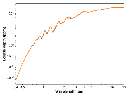
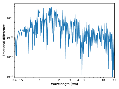
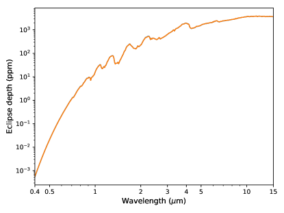
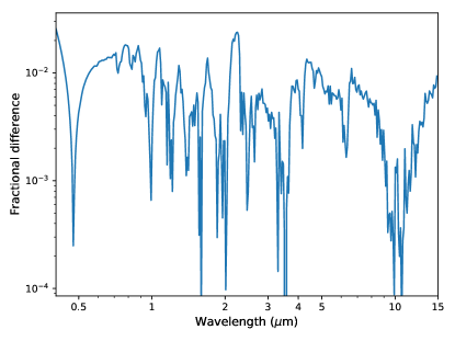
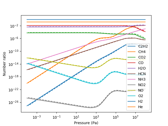
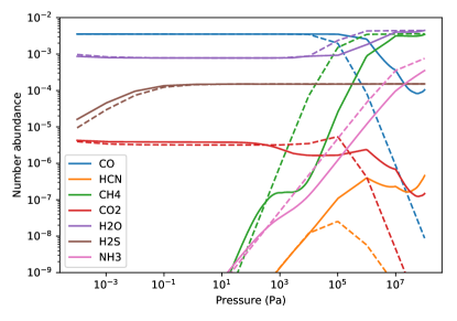
There are a number of differences between PLATON and Tau-REx that could explain the discrepancy in the predicted eclipse depths. First, PLATON performs radiative transfer at a spectral resolution of R=1000, while we ran Tau-REx with R=15,000 opacity files. Second, the two codes also handle equilibrium chemistry differently. Tau-REx uses ACE (Agúndez et al., 2012) and only considers the elements H, He, C, O, and N and 106 molecules composed of those elements, while PLATON also includes F, Na, Mg, Si, P, S, Cl, K, Ti, and V, along with 300 molecules composed of those elements. This results in abundance differences in the tens of percent, as seen in Figure 4. Third, PLATON also uses a wavelength-dependent radius to convert emergent flux to luminosity (Equation 7), but Tau-REx does not. Fourth, PLATON’s opacities are generated from newer line lists than the opacities currently available from Tau-REx’s website. Finally, there are slight differences in the algorithm used to calculate the planet-star flux ratio. For example, in calculating the emergent flux (Equation 1), Tau-REx evaluates the integral over viewing angles by sampling four viewing angles and using Gaussian quadrature, whereas PLATON evaluates the integral analytically, which is equivalent to using an infinite number of viewing angles.

Table 3Effect of removing differences between PLATON and TauREx

Removed differences	Median diff. (%)	95th percentile diff. (%)	Max diff. (%)
None	2.2	19	37
Resolution	1.2	7.6	22
Resolution, Chemistry	1.2	4.6	11
Resolution, Chemistry, Opacities	0.6	1.7	2.7
Chemistry, Opacities	1.9	17	30
Chemistry, Opacities with ktables	2.1	8.1	20

To disentangle which factors cause most of the differences, we modified PLATON step by step to more closely approximate Tau-REx’s algorithm, re-measuring the discrepancies at each step. The results are summarized in Table 3, and described in detail below. First, we replaced the default R=1000 opacities with R=10,000 opacities, which are also publicly available. This reduced the median absolute difference between Tau-REx and PLATON from 2.1% to 1.6%, with the 95th percentile at 7.4% and some wavelengths having a discrepancy of up to 17%. We conclude that a higher resolution leads to significant improvement in the agreement between PLATON and Tau-REx at some, but not most, wavelengths. Next, we disabled equilibrium chemistry and set constant abundances with altitude for CH₄, CO₂, CO, H₂O, NH₃, H₂, and He. This results in a median difference of 1.1% with a 95th percentile of 5.1% and maximum discrepancies of up to 10%. Following this, we replaced the line absorption cross sections in Tau-REx with those used in PLATON. This decreased the median difference to 0.8%, the 95th percentile to 2.1%, and the maximum difference from 10% to 2.7%. The spectra produced by the two codes are compared in Figure 3. The remaining discrepancies are likely due to slight differences in the radiative transfer code, especially the number of viewing angles (4 in Tau-REx vs. infinite in PLATON) and the precise interpolation method for absorption cross sections. As a final step, we replaced the R=10,000 opacities with the default R=1000 opacities and redid the comparison. This time, we obtained a median difference of 1.9%, a 95th percentile of 15%, and a maximum of 31%. If we do the test with correlated k radiative transfer instead of opacity sampling, these numbers are 2.2%, 7.4%, and 19%.

Based on these tests, we concluded that differences in resolution, chemistry and opacities are all significant contributors to the discrepancies between the two codes. As shown in Table 3, the median error caused by these differences are on the order of 2%, with the 95th percentile being 10-20%, and the maximum difference being a few tens of percent.

Figure 4.— Differences in molecular abundances under equilibrium chemistry conditions between GGchem (used by PLATON) and ACE (used by Tau-REx) for the test planet, with the T/P profile shown in the upper panel. These differences are typically tens of percent.

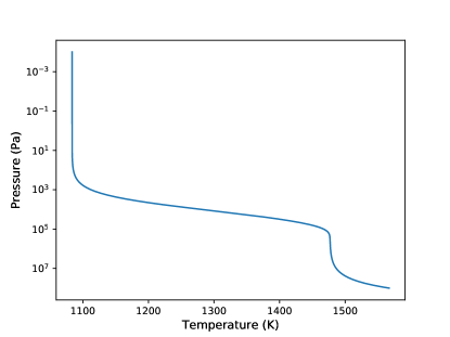
2.5. Retrieval comparison

To test the validity of PLATON retrievals, we performed an equilibrium chemistry retrieval comparison between PLATON and TauREx using a synthetic spectrum. We used TauREx to generate the 0.4–6 $\mu m$ emission spectrum using the stellar and planetary parameters in Table 2. The spectrum is binned down to a resolution of R=100, and 100 ppm of white noise is added to every binned eclipse depth. We then ran a retrieval on the synthetic spectrum using both TauREx and PLATON, with 6 free parameters (corresponding uniform priors, all generously wide, in brackets): $\log{Z}$ (-1–3), C/O (0.2–2.0), $\log{\kappa_{th}}$ (-3.4 – -1.4), $\log{\gamma_{v_{1}}}$ (-1 – 1), $\log{\gamma_{v_{2}}}$ (-1 – 1), and $\alpha$ (0–0.5). The PLATON retrieval used gas-only equilibrium abundances rather than the default condensation equilibrium abundances, while the stellar spectrum was set to a blackbody in both codes in order to ensure that any differences in the results were due to differences in the planet model and not the stellar model. We utilized nested sampling with 1000 live points for all retrievals. For PLATON, the package we used was dynesty (Speagle, 2020); for TauREx 3, it was nestle.

We ran two comparisons. In the first comparison, we generated the emission spectrum using PLATON R=10,000 opacities, and included the same set of molecular opacities in both the PLATON and TauREx retrievals: NH₃, CH₄, CO, CO₂, and H₂O. In PLATON, the opacities of all other molecules were set to 0. Figure 5 shows the results of this first retrieval comparison. In general, the two codes give very similar posteriors. The 1D posteriors of $\log_{\gamma_{v_{1}}}$, $\log_{\gamma_{v_{2}}}$, and $\alpha$ are indistinguishable. The log(Z) and C/O posteriors show discrepancies at the 0.7$\sigma$ level because the equilibrium abundances of active gases differ by a few tens of percent between PLATON and TauREx, which in turn is because the former includes many times more atoms and molecules in its calculations than the latter (see Subsection 2.4). As a result of these differences, PLATON prefers slightly higher temperatures at a given pressure ($\Delta T\sim$30 K at 100 mbar), which is reflected in the slightly higher $\kappa_{th}$.

Figure 5.— Posterior distributions retrieved by PLATON (orange) and TauREx (blue) when both codes use the same opacities and include the same list of molecules. The contours contain 68% and 95% of posterior mass. The numbers on top of each column show the values inferred by PLATON. The teal horizontal and vertical lines show the truth values.

Figure 6.— Same as Figure 5, but for the second comparision. Here, TauREx opacities are used to generate the spectrum and for TauREx’s retrieval. The PLATON retrieval uses its own opacities, with all molecules included. The discrepancy is due to the inclusion of H₂S in PLATON, but not in TauREx.

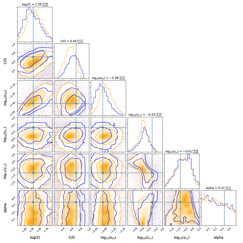
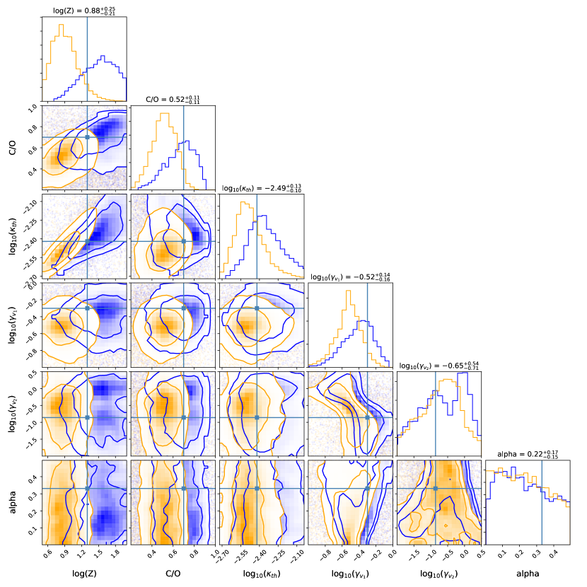
In the second comparison, we generated the emission spectrum using TauREx R=15,000 opacities and used those same opacities in the TauREx retrieval. For the PLATON retrieval, we used the the full list of molecules with the same R=10,000 opacities as in the previous comparison. The differences between the two retrievals therefore reflect both the effect of including different numbers of molecules, and differences in the line lists used for those molecules. Figure 6 shows the results of this second retrieval comparison. Even though the PLATON 1D posteriors are still consistent with the input planet parameters at the 1.7$\sigma$ level, they are more discrepant than in Figure 6, with PLATON obtaining a metallicity 4$\times$ lower and a C/O ratio 0.18 lower than the TauREx retrieval.

Having obtained this result, the natural question to ask is what causes the discrepancy: PLATON’s newer line lists, or its inclusion of more molecules? The answer is the latter. We examined PLATON’s best fit model and found that it underestimated the planetary emission around 3.8 µm, where an opacity window caused a spike in planetary emission. Removing molecules one by one from the atmosphere, we find that H₂S is the cause of the discrepancy: removing it alone from the atmosphere makes the best fit spectrum line up perfectly with TauREx’s simulated data. Indeed, when we repeat the PLATON retrieval while including only the molecules that TauREx includes, the resulting posteriors are almost identical to those of Figure 5. This underscores the importance of erring on the side of caution when choosing which active gases to include in a model. Emission spectroscopy has the inconvenient property that it is the lack of absorption that causes the most easily detectable emission–and so even a trace gas with a relatively low opacity can have a significant impact on the spectrum at wavelengths where other gases also have less absorption.

3. Opacity update

One fundamental building block of any atmospheric code is the calculation of opacities. There are three types of opacities we consider: scattering, line, and collisional. As discussed in Zhang et al. (2019), scattering opacities are calculated by PLATON itself, and collisional opacities are calculated using the limited data available from HITRAN (Richard et al., 2012; Karman et al., 2019). Line opacities are calculated from lists of transitions from one quantum state to another, giving the position, intensity, and broadening parameters of the transitions. For this update to PLATON we focused on line opacities.

In the original PLATON release, our opacity data were taken directly from Exo-Transmit (Kempton et al., 2017). Exo-Transmit, in turn, calculated its opacities from line lists generated from a large number of sources, listed in Table 2 of Lupu et al. (2014). These include HITRAN, HITEMP, private communications, Freedman et al. (2008), and Freedman et al. (2014), among many others. Many of these line lists are outdated, proprietary, or both. In addition, the program used to generate opacity data from the line lists is not public, making it difficult to reproduce our opacity calculations.

Table 4Sources of line lists

Source	Molecules
ExoMol	C2H4, CO, H2CO, H2S, H2O, HCl, HCN, MgH, NH3, NO, OH, PH3, SH, SiH, SiO, SO2, TiO, VO
HITRAN 2016	C2H2, C2H6, HF, N2, NO2, O2, O3, OCS
CDSD-4000	CO2
Rey et al 2017	CH4
NIST	Na, K

We address these shortcomings by regenerating PLATON’s opacity data using the public line lists in Table 4. For each molecule, we generate absorption cross sections from line lists using the method outlined in ExoCross (Yurchenko et al., 2018). The cross sections are generated for 30 temperatures ($100-3000$ K in 100 K increments), 13 pressures ($10^{-4}-10^{8}$ Pa in decade increments), and 4616 wavelengths ($0.3-30$ µm, with uniform spacing in logarithmic space). The resolution of our wavelength grid is not high enough to resolve individual lines at typical atmospheric pressures (P $<$ 1 bar), leading to spikiness in the wavelength-dependent cross sections, and therefore in the final transit and secondary eclipse depths. This approach to radiative transfer is called “opacity sampling”. The idea behind opacity sampling is that even though the sampling resolution is much lower than that needed to resolve individual lines, it is still much higher than the instrumental resolution, and the spikiness in the resulting models can be smoothed out by binning to instrumental resolution.

We generate cross sections by assuming a Voigt profile for every line, with the Gaussian standard deviation set by the temperature of the gas, and the Lorentzian portion set by the pressure broadening coefficients $\gamma_{\rm ref}$ and $n$:

$$\gamma(P,T)=\gamma_{\rm ref}\frac{P}{P_{ref}}\bigg{(}\frac{T_{\rm ref}}{T}\bigg{)}^{n}$$ (14)

where $\gamma_{\rm ref}$ and $n$ are expected to vary depending on the line considered and the species responsible for the broadening.

3.1. ExoMol

ExoMol (Tennyson & Yurchenko, 2018) is a database of molecular line lists intended for modeling the atmospheres of exoplanets and cool stars. The lists are generated using a combination of ab initio calculations and empirical data. Many of the line lists represent significant improvements in completeness over the previous state of the art. For example, POKAZATEL, the water line list, has 6 billion transitions. This is an order of magnitude more than previous lists, and covers every possible transition between states below the dissociation energy of water (Polyansky et al., 2018). Compared to the Freedman et al. (2008) line lists used by previous versions of PLATON, the ExoMol line list has many times the number of transitions for water (6 billion vs. 200 million), NH₃ (10 billion vs. 34,000), H₂S (115 million vs. 188,000), PH₃ (50 billion vs. 20,000) and VO (377 million vs. 3.1 million).

The specific line lists we used are listed in Table 10, together with the number of transitions they contain, their maximum temperature of validity, and citations to the associated papers. For some molecules, ExoMol provides line lists for multiple isotopologues; in those cases we only include the most common isotopologue. The exception to this rule is TiO, an important molecule where multiple isotopologues have comparable abundances. For this molecule, we compute the absorption due to each isotopologue and add them in proportion to each isotopologue’s abundance.

Although these ExoMol line lists are an improvement over what was available before, many are still incomplete. The calculations only include states below a certain $J$ quantum number, and hence miss transitions between higher-energy states that become important at higher temperatures. Thus, many line lists are not valid for the full range of temperatures supported by PLATON, which ranges up to 3000 K. For example, the C₂H₄ line list, despite having 50 billion lines, is only valid below 700 K. For these molecules, we still generated cross sections for all temperatures. The cross sections are likely to be under-estimated at high temperatures due to missing lines, but as of this writing, there is no better alternative.

ExoMol reports line broadening coefficients for hydrogen and helium whenever available. In practice, however, there are no calculations or experimental data available for any broadening agent for the vast majority of lines. For example, ExoMol reports no broadening coefficients at all for H₂S, CO, MgH, NO, OH, SiH, SiO, or VO. For NO, it only reports air broadening coefficients, which we adopt for lack of a better alternative. For the other molecules, ExoMol reports broadening coefficients for H₂ and He in a consistent format (Barton et al., 2017), relying on the handful of studies that have reported coefficients for a small number of lines while resorting to default values for the rest. We used ExoMol broadening data when available and assumed that the broadening agent is a mixture of 85% H₂ and 15% He. For all molecules where ExoMol broadening data is not available, we assumed that $\gamma_{ref}=0.07$ and $n$=0.5 at a $T_{\rm ref}=296K$ and $P_{ref}$ = 1 bar. $n$=0.5 is the theoretically expected value from classical calculations, while $\gamma_{ref}=0.07$ is a typical value adopted by ExoMol as the default. The only exception is C₂H₄, where we used broadening parameters measured by Bouanich et al. (2003) (H₂) and Reuter & Sirota (1993) (He) for 34 and 3 lines respectively by generating ExoMol-formatted broadening files from the measurements.

3.2. HITRAN 2016

HITRAN (Gordon et al., 2017) is a database of line lists sourced from a combination of observations, theory, and semi-empirical calculations. It is intended for use at terrestrial temperatures, and has a line intensity cutoff that makes it inaccurate for higher temperatures. Nevertheless, HITRAN is a valuable resource because it is the only source of line lists for many molecules. HITRAN specifies line broadening parameters by including $\gamma$ and $n$ in the description of every line. Although $\gamma_{H2}$ and $n_{H2}$ are included in HITRAN, very few lines have hydrogen broadening data. Therefore, we chose $\gamma_{air}$ and $n_{air}$ as the broadening parameters for every line.

For most molecules not included in ExoMol, Exo-Transmit used (and PLATON inherited) absorption data from HITRAN 2008. We regenerate the absorption data using HITRAN 2016 (Gordon et al., 2017), which has expanded wavelength coverage and improved accuracy. This update also fixed some errors in the old data that resulted from incorrect generation of absorption data from line lists. The HAPI API makes it easy to retrieve line lists for all isotopologues at once, with intensities appropriately scaled to the isotopologue abundance. Therefore, we considered all isotopologues for the molecules we took from HITRAN.

3.3. CDSD-4000

The Carbon Dioxide Spectroscopic Databank 4000 (CDSD-4000) is a line list meant for high temperatures, provided in a format similar to HITRAN. It has significantly more lines than HITRAN or HITEMP, and to our knowledge it is the most complete publicly available line list for carbon dioxide. CDSD-4000 has pressure broadening coefficients for air, which we adopt due to the absence of broadening coefficients for hydrogen or helium.

3.4. Rey et al 2017

The line list presented by Rey et al. (2017), which we name Rey for convenience, is the first theoretical methane line list suitable for high temperature applications. It is complete in the infrared range (0–13,400 cm^-1) up to a temperature of 3000 K, whereas the ExoMol line list “10to10” is only accurate to 1500 K (Yurchenko & Tennyson, 2014). Rey also claims to be the first theoretical methane line list with line positions accurate enough for high resolution cross-correlation studies. We have confirmed this claim by cross correlating brown dwarf models generated using both methane line lists to observational high-resolution spectra of a T brown dwarf, with all other opacity sources excluded. The cross correlation peak is 4.5$\sigma$ with “10to10”, but 15.3$\sigma$ with Rey, indicating far superior line positions. In addition, with 150 billion lines, this line list is far more complete than either ExoMol’s “10to10” line list (10 billion transitions) or the Freedman et al. (2008) line list that we used previously (200 million transitions).

3.5. Voigt cutoff

When generating absorption cross sections from line lists, the cutoff–namely, how far away from the line center the line is considered to end– is an important source of error. One could in principle omit the cutoff, but computational speed would suffer greatly. In addition, omitting the cutoff does not necessarily lead to better results, as the Voigt profile is only an approximation to the true line profile (Ngo et al., 2012) and is not accurate more than several Voigt widths away from the center. However, truncating the lines too soon would result in an underestimate of the true opacity due to the omission of millions of line wings.

We adopted a cutoff of 25 cm^-1 for all molecules for pressures less than or equal to 1 bar. For pressures of 10 and 100 bar, we adopted a cutoff of 100 cm^-1. For a pressure of 1000 bar, we adopted a cutoff of 1000 cm^-1. This prescription was inspired by Sharp & Burrows (2007), who adopt a cutoff of min(25$P$, 100) cm^-1 where P is in bars. Hedges & Madhusudhan (2016) studied the effect of different cutoffs and concluded that the Sharp & Burrows prescription significantly underestimates absorption at low pressures (P $<$ 0.01 bar), but is accurate from 0.01 to 100 bar. We therefore modified the prescription to use 25 cm^-1 for all pressures below or equal to 1 bar. Pressure broadening coefficients are almost never measured or calculated at very high pressures ($100-1000$ bar), so our opacity data in this regime should be regarded as highly speculative.

4. Other improvements

Aside from the opacity update and the eclipse depth calculator, many improvements have been made to PLATON since the publication of the last paper. These improvements introduce features, fix bugs, increase speed, and improve usability. A comprehensive list can be found in our release notes, but we list a few of the most noteworthy updates below.

• We now include H- opacity, calculated using the algorithm in John (1988). Because H- opacity is insignificant for most planets, we disable it by default.

• Nested sampling is now done by dynesty (Speagle, 2020) rather than nestle. Among other improvements, dynesty prints out the number of likelihood evaluations, log evidence (logz), and remaining evidence (dlogz) after each iteration. dlogz is an indicator of how far the algorithm is from completion. nestle did not have this indicator, which made waiting a frustrating experience.

• The eclipse depth calculator now evaluates the single integral in Equation 2 instead of the double integral in Equation 1, making it much faster, many times more memory efficient, and more accurate.

• Data arrays are transposed so that the wavelength index increases the fastest, followed by the pressure index, followed by the temperature index. This improves cache locality, which speeds up the code by a factor of 1/3.

• The number of atmospheric layers is decreased from 500 to 250, improving speed by 40% while increasing numerical error by only $\sim$1%. In addition, we now use improved interpolation methods to further decrease numerical errors.

4.1. High resolution opacities

PLATON has a clean separation between data and code. As a result, all that is needed to operate PLATON at an arbitrary wavelength range and resolution is the appropriate opacity data files. No code changes are required. Since we published Zhang et al. (2019), we have generated high-resolution opacity data files for a variety of applications. This includes studying the atmospheres of cold brown dwarfs, of the ultra-hot super Earth 55 Cnc e, and of HD 189733b (see Subsection 5.9).

We now make these opacities public to enable anyone to perform line-by-line calculations with PLATON . All opacities have a resolution of R=375,000, and are calculated at the wavelengths indicated by wavelengths.npy. These opacities can be used by deleting all files from the “Absorption” folder in PLATON’s data directory, putting the downloaded absorb_coeffs files into the directory, and replacing the wavelengths.npy file in the data directory with the one in the downloaded zip file. The user must use a blackbody stellar spectrum (by passing stellar_blackbody=True to compute_depths) when using high resolution opacities. The user can also generate their own high-resolution opacity files using publicly available codes such as ExoCross (Yurchenko et al., 2018) or HELIOS-K (Grimm & Heng, 2015). As long as they are in the same format as the PLATON data files, PLATON will accept them with no code changes.

Table 5High resolution absorption data

Filename	Wavelengths (µm)	Molecules
hispec	$0.94-2.43$	CH4, CO, H2O, H2S, HCl, HCN, MgH, NH3, NO2, NO, O2, O3, OH, SH, SiH, SiO, SO2, TiO, VO
$Y$_band	$1.020-1.086$	CH4, H2O, NH3
$K$_band	$1.89-2.40$	C2H2, CH4, CO, H2O, HCN, Na, NH3, SiO
$L$_band	$2.86-3.70$	C2H2, CH4, CO, H2O, H2S, HCN, Na, SiO
$L$_band2	$3.51-4.08$	CH4, CO2, H2O, HCN

We note that in principle other codes, such as TauREx, can also be used to calculate high resolution spectra if they are provided with custom user-generated high resolution opacity files. To the best of our knowledge, however, PLATON is the only code to make such opacity files publicly available.

4.2. Correlated-$k$

The gold standard of radiative transfer is the line-by-line method (Marley & Robinson, 2015): calculating the transit or eclipse depth on a wavelength grid fine enough to resolve individual molecular lines, which typically requires $R>>c/\sqrt{\frac{kT}{\mu m_{H}}}\approx 200,000$. The results are then binned to instrumental resolution. For many applications, including PLATON, this is computationally prohibitive. Opacity sampling sacrifices accuracy for speed by performing radiative transfer at a much lower resolution–R=1000, in the case of PLATON–and binning the depths thus obtained to instrumental resolution. In order for the survey to approximate the results of the census, a large sample size is required, meaning opacity sampling at R=1000 is only accurate if the user is binning to resolutions much below 1000. To take a concrete example, suppose PLATON is used to calculate the eclipse depth of HD 189733b over the 1.40–1.42 µm band using the R=10,000 opacities. PLATON would sample 140 wavelengths within this band and calculate the eclipse depth at each wavelength. These 140 eclipse depths would have a mean of 53 ppm and a standard deviation of 25 ppm. Therefore, the error caused by opacity sampling is $25/\sqrt{140}$=2 ppm. If the R=1000 opacities were used instead, this error would be $25/\sqrt{14}=7$ ppm. Fortunately, 7 ppm is several times lower than the error of the WFC3 observations, but this will not be the case for every combination of planet, instrument, and wavelength band.

The correlated-$k$ method (Lacis & Oinas, 1991) improves upon opacity sampling by taking into account the distribution of opacities within the passband. For example, it calculates the 10th percentile eclipse depth by using the pre-calculated 10th percentile of all molecular opacities, and likewise for the 20th percentile, 30th percentile, etc. Since the eclipse depth varies smoothly with percentile, we can use numerical integration to find the average eclipse depth. In effect, the correlated-$k$ method converts an integration over wavelength into an integration over percentile; it replaces the integration of a highly non-smooth function $\int_{\lambda_{1}}^{\lambda_{2}}{f(\lambda)d\lambda}$ with the integration of a smooth function $\int_{0}^{1}{f^{\prime}(g)dg}$, which is in turn evaluated by Gaussian quadrature ($\sum_{i=1}^{N}{w_{i}f^{\prime}(g_{i})}$), where g is the percentile divided by 100. $f(\lambda)$ can be $R_{p}(\lambda)$, the emergent flux $F_{p}(\lambda)$, or any other radiative quantity, so long as its only dependence on wavelength is through the opacity, and so long as it varies smoothly with opacity.

Earlier versions of PLATON performed radiative transfer via opacity sampling at a default resolution of 1000 with an optional R=10,000 mode. We now give the user the option to choose between correlated-$k$ (R=100) and opacity sampling. The correlated-$k$ method provides the accuracy of R=50,000 opacity sampling for typical exoplanet applications, but runs at the same speed as the old default R=1000 PLATON mode. Our implementation of correlated-$k$ rests on two approximations:

1. At any given wavelength $\lambda$ within the band, $g(\lambda)$ is the same for every layer. That is, if a layer is more opaque at a certain wavelength than at x% of other wavelengths within the band, all other layers must also be more opaque at that wavelength than at x% of other wavelengths.

2. For each layer, if the individual gases were to be separated out, $g(\lambda)$ would be equal for all gases with significant opacity. That is, if one molecule absorbs more strongly at a certain wavelength than at x% of other wavelengths within the band, the same must be true for all other molecules.

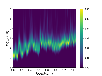
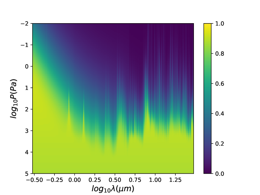
The first assumption is the defining assumption of the correlated-$k$ method, and explains its name: the opacity $\kappa$ is assumed to be correlated throughout the atmosphere under consideration. For an atmosphere with one species with exactly one absorption or emission line within the band, it is exactly true. For an atmosphere with two layers, each of which is exclusively composed of a different gas, it is very inaccurate. A real atmosphere is in between these two extremes: the region dominating the features in a transmission or emission spectrum typically spans $\sim$200 K in temperature (Figure 10) and 1-2 orders of magnitude in pressure (see Figure 10 and 11), which generally means that there is no change in the dominant gas absorber.

The second assumption, however, is only true when one molecule dominates the opacity. If two molecules contribute equally to the opacity, the assumption is no longer valid, as the absorption lines of different molecules will not in general overlap. In fact, the opposite assumption is more accurate: namely, that the opacities are completely uncorrelated between different gases. Lacis & Oinas (1991) take this approach, but adopting this assumption naively for PLATON would require O($n^{N}$) radiative transfer calculations, where $n$ is the number of discrete $g$ values adopted (for us, 10) and $N$ is the number of gases (for us, 30), making these computations intractable. There are methods of merging the opacity distributions of multiple gases that do not scale exponentially–including the ‘random overlap with resorting and rebinning’ method introduced by Lacis & Oinas (1991) and named by Amundsen et al. (2017). These are more complicated to implement, and we may incorporate them into a future release of PLATON. The partially correlated approach attempts to take into account the correlations between gases (Zhang et al., 2003), but these sophisticated schemes are beyond the scope of PLATON.

We note that the simplicity of our approach comes at a cost: it systematically overestimates transmittance in most cases (Zhang et al., 2003). This overestimation is easy to understand with a toy scenario. Consider a gas with binary absorption properties: at 50% of wavelengths it has infinite absorption, while at the other wavelengths it has zero absorption. This gas would have a transmittance of 50%. Now consider adding a second gas, also with binary absorption properties. If the two gases have perfectly correlated absorption (which is our assumption), their absorption peaks fall on top of each other, and transmittance is still 50%. If their absorption is not perfectly correlated, the absorption peaks of the second gas block some of the light that would have went through the first gas, and total transmittance is less than 50%. If their absorption is perfectly anti-correlated, the total transmittance would be 0%.

In practice, PLATON uses the following correlated-$k$ algorithm:

1. (Pre-computed) Compute the absorption coefficients of each atom/molecule at each temperature, pressure, and wavelength grid point, with a spectral resolution of R=50,000. Correlated-$k$ coefficients are generated from the absorption coefficients with a resolution of R=100.

2. Divide the wavelength range under consideration into bands, with each band having a width of $\lambda/100$

3. For each band, compute the transit/eclipse depth at 10 different opacity percentiles, and combine them via Gaussian quadrature. The transit depth at the 16th opacity percentile (for example) is calculated by assuming every gas, at every temperature and pressure, has an absorption coefficient equal to the pre-calculated 16th percentile absorption coefficient for that band at that temperature and pressure. We use 10 Gaussian quadrature points, which is sufficient to keep the integration error below 1% in most cases (Lacis & Oinas, 1991; Goody et al., 1989).

4. The R=100 transit or eclipse depths are then binned to the user-specified wavelength bins using the methods described in our first paper (Zhang et al., 2019).

We performed an experiment to deduce the accuracy of the correlated-$k$ algorithm compared to a line-by-line calculation. The transit spectrum of a hot Jupiter (modelled after HD 209458b) was computed from $0.95-2.4$ µm using two methods: a line-by-line calculation at R=375,000 binned to R=100, and a correlated-$k$ calculation using R=100 opacities with 10 Gaussian quadrature points. For the nominal model, which is dominated by water opacity, correlated-$k$ performs extremely well and has a maximum error of only 8 ppm. For a model engineered to include three molecules with comparably significant absorption correlated-$k$ still performs well, with a maximum error of 300 ppm. The emission spectrum tells a similar story. Correlated-$k$ is accurate to 0.1% for the nominal model, and to 3.5% for the pessimistic model.

These tests also demonstrate that although correlated-$k$ is very accurate, its errors are not random. Correlated-$k$ almost always underestimates the transit depths and overestimates the eclipse depths. This is a consequence of overestimating the transmittance, which in turn is because (contrary to the second assumption above) the absorption properties of two molecules are in general not strongly correlated.

4.3. Beta features

Since we do not currently plan to write a third PLATON paper, we include a list of beta features that will likely become part of the official PLATON. This list also serves to illustrate what is possible with minimal hacking. All of these features were created as a result of requests from PLATON users other than the authors. Users are highly encouraged to contact the authors to suggest new features or improvements to existing features.

PLATON does not calculate disequilibrium chemistry from first principles, nor does it compute self-consistent temperature-pressure profiles. It is often useful to take abundance and temperature profiles from elsewhere and plug them into PLATON, using it as a radiative transfer engine to predict transit and eclipse depths. This is currently easy to do for vertically-constant abundances, but not for vertically-variable abundances. To make the latter possible, we created the branch custom_abundances on the GitHub repository. Examples of how to use it are found in examples/plot_transit_custom_abunds.py and examples/plot_eclipse_custom_abunds.py.

Some metallic species are not included in PLATON by default, but may become important in the optical for ultra-hot Jupiters. These include Ca, Fe, Ni, and Ti. We make these opacities available at https://www.astro.caltech.edu/platon/metal_opacities/. These can be used by placing them in PLATON_DIR/data/Absorption and adding the atoms to PLATON_DIR/data/species_info. These atoms are not incorporated into the equilibrium chemistry calculation, but the user can easily specify vertically constant abundances for them. We describe the procedure in PLATON’s online documentation.

Lastly, Na and K each have two very strong lines in the optical, where the atmosphere is transparent enough that their far wings may become significant. Unfortunately, while the lines cores are accurately described by a Voigt profile, the Voigt profile can underestimate far wing absorption by orders of magnitude (Allard, N. F. et al., 2016; Allard et al., 2019). More accurate line profiles for these atoms were recently published by Allard, N. F. et al. (2016) (K) and Allard et al. (2019) (Na) using a semi-classical theory and assuming broadening by molecular hydrogen only. We use these line profiles to generate PLATON-friendly absorption coefficients at R=1000 and R=10,000, found at https://www.astro.caltech.edu/platon/metal_opacities/. By overwriting PLATON_DIR/data/Absorption/absorb_coeffs_Na.npy and PLATON_DIR/data/Absorption/absorb_coeffs_K.npy with these coefficients, the user can generate much more accurate hydrogen-broadened alkali line profiles with PLATON.

5. Retrieval on HD189733b

5.1. Published data sets

HD 189733b is one of the most favorable exoplanets for atmospheric characterization. It is a transiting hot Jupiter orbiting an exceptionally close (20 pc) K star with a $H$ band magnitude of 5.6, and was one of the earliest transiting planets discovered (Bouchy et al., 2005). To demonstrate PLATON’s new abilities, we perform a joint retrieval on the best available optical and near infrared transit and secondary eclipse data for HD 189733b from HST and Spitzer. To our knowledge, this is the first joint transit and secondary eclipse retrieval for this planet in the literature, as well as the most comprehensive set of both transit and secondary eclipse data assembled for a retrieval to date. The fixed stellar and planetary parameters are listed in Table 7. The transit depths we adopt are listed in Table 8, while the eclipse depths are listed in Table 9.

HD 189733b has been observed in transmission with HST/STIS (Sing et al., 2011) and WFC3 (Gibson et al., 2012; McCullough et al., 2014), Spitzer in all five IRAC bands (Tinetti et al., 2007; Beaulieu et al., 2008; Agol et al., 2010; Désert et al., 2011; Morello et al., 2014), and Spitzer/MIPS at 24 µm (Knutson et al., 2009). Pont et al. (2013) carried out a uniform re-analysis of all transit data obtained to date including corrections for stellar activity; we utilize their transmission spectral data in our analysis. This planet was also observed in transit by HST/NICMOS in spectroscopic (Swain et al., 2008) and photometric (Sing et al., 2009) modes, but this instrument was less stable than WFC3, and the reliability of the spectroscopic NICMOS observations was questioned in a subsequent study (Gibson et al., 2011; Deming & Seager, 2017). We therefore exclude these older NICMOS observations from our analysis. We also exclude the higher resolution observations of the sodium line published in (Huitson et al., 2012), as PLATON is not designed to model absorption at the very low pressures probed by the core of this line.

In emission, HD 189733b has been observed with HST/STIS (Evans et al., 2013), HST/NICMOS (Swain et al., 2009), HST/WFC3 (Crouzet et al., 2014), Spitzer/IRAC in all four bands (Knutson et al., 2007; Charbonneau et al., 2008; Agol et al., 2010; Knutson et al., 2012), Spitzer/IRS at $5-14$ µm (Deming et al., 2006; Grillmair et al., 2008; Todorov et al., 2014), and Spitzer/MIPS at 24 µm (Knutson et al., 2009). Because PLATON does not model reflected light, we limit our retrieval to the infrared data only, which are expected to be dominated by thermal emission. As with the transmission spectrum, we exclude the NICMOS observations from our retrieval. We also exclude the Spitzer/IRS emission spectrum, as over the years different groups have obtained contradictory results. Most recently, Todorov et al. (2014) found that the overall amplitude of the IRS eclipse depth can shift up and down depending on the method used to correct for systematics. Indeed, a comparison to our best fit model spectrum reveals that these data are consistent with the broadband observations if they are shifted upwards by 30%. In addition to transit and secondary eclipse observations, HD 189733b’s phase curve has also been measured in the 3.6, 4.5, 8.0, and 24 µm Spitzer bands (Knutson et al., 2007, 2009, 2012).

Based on the observations listed above, HD 189733b is one of the most extensively observed transiting planets to date. Previous studies of HD 189733b’s optical transmission spectrum found that it appears to have a strong scattering slope and attenuated absorption features due to the presence of high-altitude scattering particles (Pont et al., 2008; Sing et al., 2011; Pont et al., 2013). These scattering particles are possibly some form of silicate condensate (Lecavelier Des Etangs et al., 2008; Lee et al., 2015; Helling et al., 2016). Because this planet is expected to be tidally locked, it should develop a super-rotating equatorial band of wind that transports heat from the day side to the night side (e.g., Showman & Polvani 2011). It is observed to have a relatively modest day-night temperature gradient (Knutson et al., 2007, 2009, 2012) and models predict that it may also have spatially inhomogeneous cloud coverage (Lee et al., 2015; Lines et al., 2018).

In the infrared the effect of the scattering particles on HD 189733b’s transmission spectrum is reduced. McCullough et al. (2014) report the detection of a spectroscopically resolved water feature at 1.4 µm that is consistent with the model of scattering aerosol reported by Pont et al. (2013), although they also argue that the optical slope can be explained by stellar activity alone (see Section 5.7). In emission, previous studies have detected spectroscopically resolved water absorption at 1.4 µm (Crouzet et al., 2014) and (debatably) in the mid-infrared (Grillmair et al., 2008; Todorov et al., 2014), and have placed additional constraints on the abundances of carbon monoxide, carbon dioxide, and methane based on the relative depths of the broadband Spitzer secondary eclipse data (e.g., Line et al. 2010; Lee et al. 2012). We discuss the results of these retrievals in more detail in Section 5.3.

5.2. PLATON retrieval

When modeling HD 189733b’s transmission spectrum, our retrieval uses a complex refractive index with a real component of 1.7, a value in between that of MgSiO₃ and SiO₂ (which have $n\sim 1.5$ at optical wavelengths) and TiO₂ (which has $n\sim 2.4$). Since the true composition of condensates in the atmosphere is unknown, and multiple condensates may well be important, we allow the imaginary component of the refractive index to vary as a free parameter in our fit. We do not include clouds in our dayside models; even if the clouds observed on the terminator extended over the entire dayside, we would expect them to have lower optical depths when viewed in emission at infrared wavelengths (e.g., Fortney 2005). Indeed, previous retrieval studies of HD 189733b’s dayside atmosphere have found that cloud-free models provide a good fit to the available data (e.g. Barstow et al. 2014).

Figure 7.— Top: Best fit transit spectra from retrieval on HD 189733b. The best-fit PLATON model and corresponding $1\sigma$ uncertainty window are shown as a red line and red shaded region, respectively. The activity-corrected observations drawn from Pont et al. (2013) and listed in Table 8 are shown as black filled circles. Bottom: difference between observed and computed transit depths, in units of measurement error $\sigma$. Adopting the nightside emission pollution correction of Kipping & Tinetti (2010) would reduce the errors on the 8µm and 24µm points by 0.6$\sigma$ and 0.4$\sigma$ respectively, bringing the observations into nearly perfect agreement with the model.

Figure 8.— Top: Best fit eclipse spectra from retrieval on HD 189733b. The best-fit PLATON model and corresonding $1\sigma$ uncertainty window are shown as a red line and red shaded region, respectively. Data used in the fit (see list in Table 9) are shown as black filled circles. The IRS eclipse depths from Todorov et al. (2014) are shown in grey and were not included in the retrieval. These eclipse depths have been shifted up by 30% to match the model–a plausible shift, since Todorov et al. (2014) mentions that its results are 20% below those of Grillmair et al. (2008). Bottom: difference between observed and computed secondary eclipse depths, in units of measurement error $\sigma$.

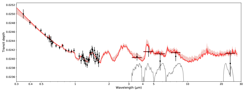
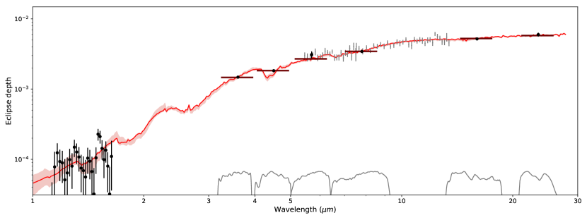
We carry out our retrievals using the dynesty nested sampling package with static sampling and R=10,000 opacities. We used 1000 live points, a convergence criteria of $\Delta$log(z) = 1, multi-ellipsoidal bounds, and a random-walk sampling method. The fixed parameters, listed in Table 7, are the stellar radius, stellar temperature, and planetary mass. The free parameters, listed in Table 6, are the planetary radius $R_{p}$ at 1 bar, the metallicity $Z$ relative to solar, the C/O ratio, the limb temperature $T_{limb}$, the Line et al. (2013) T/P profile parameters (thermal opacity $\kappa_{th}$, visible-to-thermal opacity ratio of first visible stream $\gamma$, visible-to-thermal opacity ratio of second visible stream $\gamma_{2}$, percentage apportioned to the second visible stream $\alpha$, effective albedo $\beta$), mean haze particle radius $r_{m}$, haze particle number density $n$, ratio of haze scale height to gas scale height $h_{frac}$, WFC3 instrumental offsets ($\Delta_{wfc3,t}$ for transit and $\Delta_{wfc3,e}$ for eclipse), and the imaginary portion of the haze refractive index $k$. In Figure 7 and 8, we show the best fit transit and eclipse spectra from our retrieval. Our best fit model is a good fit overall to the data, with a $\chi^{2}$ of 30.7 for the transit spectrum and 38.3 for the eclipse spectrum for a total $\chi^{2}=69$. With 52 transit depths, 34 eclipse depths, and 15 free parameters, the p value is 0.55. The single largest point of disagreement (3.1$\sigma$) between model and data occurs at the very red end of the WFC3 emission spectrum, where edge effects may impact the reliability of data.

Figure 9.— Posterior distribution of the fiducial retrieval on HD 189733b.

Table 6Retrieved parameters

Parameter	Posterior	Best	Prior
$R_{p}\textrm{ (R${}_{\textrm{J}}$)}$	$1.117\pm 0.002$	1.114	$[1.11,1.13]$
$\log_{10}Z$	$1.08_{-0.20}^{+0.23}$	0.956	$[-1,3]$
$C/O$	$0.66_{-0.09}^{+0.05}$	0.69	$[0.2,2]$
$T_{limb}\textrm{ (K)}$	$1089_{-120}^{+110}$	1203	$[500,1300]$
$\log_{10}\kappa_{th}\textrm{ (m${}^{2}$ kg${}^{-1}$)}$	$-1.40_{-0.32}^{+0.40}$	-1.44	$[-5,0]$
$\log_{10}\gamma$	$-0.51_{-0.21}^{+0.36}$	-0.66	$[-4,1]$
$\log_{10}\gamma_{2}$	$-0.58_{-0.50}^{+0.62}$	-0.47	$[-4,1]$
$\alpha^{*}$	$<0.47$	0.441	$[0,0.5]$
$\beta$	$0.95\pm 0.05$	0.938	$[0.5,2]$
$\log_{10}r_{m}$(m)∗	$<-7.8$	-8.59	$[-9,-5]$
$\log_{10}n(m^{-3})$	$16.0_{-2.7}^{+1.5}$	14.4	$[8,21]$
$h_{frac}$	$3.2_{-0.5}^{+0.6}$	3.19	$[0.5,5]$
$\Delta_{wfc3,t}\textrm{(ppm)}$	$-63\pm 28$	-72	$0\pm 100$
$\Delta_{wfc3,e}\textrm{(ppm)}$	$29\pm 9$	33	$0\pm 39$
$\log_{10}k^{*}$	$*<-1.7$	-3.86	$[-6,0]$

Figure 10.— Left: emission contribution function of HD 189733b, as indicated by the best fit solution. Right: the T/P profile as indicated by the best fit solution (red), along with the 2$\sigma$ uncertainties on the T/P profile (blue). The median limb temperature is indicated in black, while the 1$\sigma$ uncertainty in limb temperature is indicated in gray.

Figure 11.— Contribution function of the transmission spectrum. The absolute scale is in arbitrary units.

Figure 12.— Number abundances of the most common molecules in the limb (dashed) and on the day side (solid), according to the best fit model. Hydrogen and helium, the dominant components of the atmosphere, are not shown.

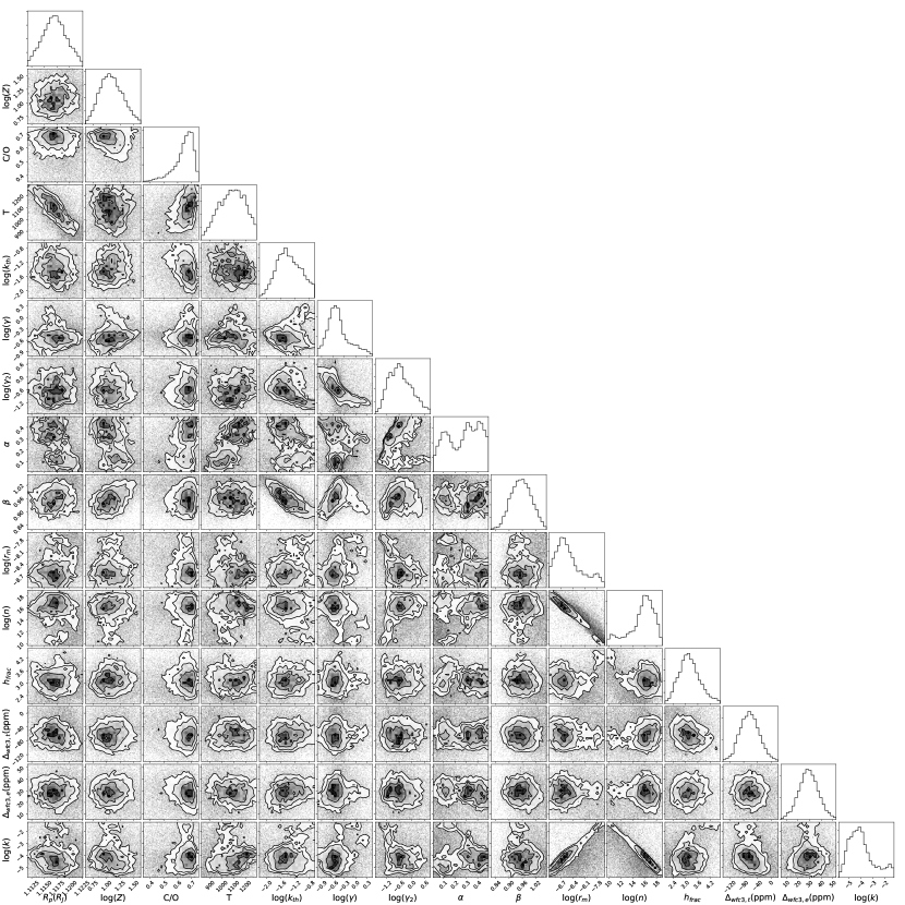
In Table 6, we tabulate the 1D posterior distributions from the retrieval. In Figure 9, we show the 2D posterior distributions. We find that the data prefer supersolar metallicities ($Z=7-20$) and a C/O ratio between $0.47-0.69$. This C/O ratio is consistent with the solar value, but is somewhat low compared to the stellar C/O ratio of $0.90\pm 0.15$ (Teske et al., 2014). However, Teske et al. (2014) also report that their estimate for the stellar C/O ratio depends on what data they include and how the non-LTE correction is performed. They report C/O ratios ranging from 0.69 to 1.2 for different data analysis choices, and conclude that although the C/O ratio could be below 0.75, it is very likely above 0.80. If so, the planetary atmospheric C/O ratio would be slightly suppressed relative to the stellar value, in good agreement with theoretical predictions for gas giant planets with atmospheric metallicities enhanced by the accretion of solids (Espinoza et al., 2017).

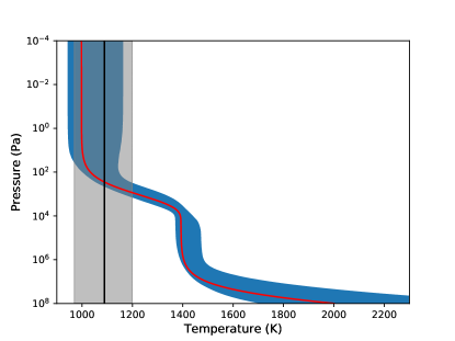
Our observations also constrain HD 189733b’s dayside pressure-temperature profile. We find no evidence for a dayside temperature inversion, as shown in Figure 10. The parameter $\alpha$, which partitions the visible radiation into two separate channels and corresponds to the flux in the channel with opacity $\gamma_{2}$, is consistent with 0. This means that there is no need for a second visible wavelength channel and that the simpler double-gray parameterization of Guillot (2010) is sufficient. We also find that the overall shape of the pressure-temperature profile is consistent with a low albedo and efficient day-night redistribution of heat, as $\beta$ is consistent with 1.

We place constraints on the sizes and locations of the scattering particles near HD 189733b’s terminator. The mean particle size is constrained to be less than 14 nm, and is consistent with arbitrarily small values. However, this size constraint is dependent on the assumed value of the imaginary refractive index, with more absorbent particles requiring a larger mean particle size (see Subsection 5.5 for more details). We find that the fractional scale height of the haze is a factor of a few larger than that of the gas. In effect, this means that haze particles are more abundant relative to gas in the upper atmosphere than in the lower atmosphere. This could possibly indicate that the haze is photochemical in nature, a possibility first suggested by Zahnle et al. (2009) and Pont et al. (2013). The fact that photochemical hazes can generate super-Rayleigh scattering slopes in the $T_{eq}=1000-1500$ K regime was recently demonstrated by Ohno & Kawashima (2020), who showed that strong eddy diffusion gives rise to a $\rho_{\rm haze}/\rho_{\rm gas}$ ratio that increases with height, which in turn leads to a steep spectral slope.

5.3. Comparison with previous retrievals

Many authors have attempted to use retrievals to constrain the atmospheric properties of HD 189733b, starting with Madhusudhan & Seager (2009). Here, we review the most recent retrievals, including Lee et al. (2014) and Pinhas et al. (2019) in transmission and Lee et al. (2012) in emission, and compare their results to ours. Although Benneke (2015) separately performed a retrieval on HD 189733b’s WFC3 transit spectrum, the limited wavelength range of these data prevented them from obtaining meaningful constraints on the atmospheric metallicity.

Lee et al. (2014) performed a retrieval on the $0.3-10$ µm transmission spectrum data reported in Pont et al. (2013). Because this study was performed prior to the publication of the WFC3 data, it used NICMOS spectroscopy to constrain the shape of HD 189733b’s near-infrared transmission spectrum. As part of this retrieval they explored several different potential aerosol species, including MgSiO₃, Mg₂SiO₄, astronomical silicate (a mixture of siliciate grains commonly seen in interstellar space), MgSiO₃, NaS, and tholins, all of which they argued might plausibly form in the upper regions of HD 189733b’s atmosphere. They found that a vertically uniform aerosol layer stretching from 0.1 mbar to 10 bar filled with monodispersed particles smaller than 0.1 µm provides a good fit to the spectrum for all aerosol compositions. This matches well with our updated fits, which indicate that the data are consistent with a large range of imaginary refractive indices and favor particles with a mean radius smaller than 14 nm, distributed with a scale height much larger than that of the gas. Lee et al. (2014) also reported a constraint of $0.02-20\times 10^{-4}$ on the abundance of water after accounting for the uncertainties introduced by different aerosol assumptions. Our best fit model is on the upper end of this range with a photospheric water abundance of $10^{-3}$, but it is consistent with the water abundances from this study for both Mg₂SiO₄ and tholin aerosols.

Pinhas et al. (2019) use AURA to perform a retrieval on the transit spectrum from STIS, ACS, WFC3, and IRAC 3.6/4.5 (0.35–4.5 µm). They obtain a water abundance of $\log(X_{H_{2}O})=-5.04_{-0.30}^{+0.46}$, which is 1.8% the equilibrium value at solar elemental abundances, and claim a strong detection of water depletion. We computed the water abundance at 10 mbar in our models, taking this to be representative of the photospheric pressure, and obtained $\log(X_{H_{2}O})=-2.5\pm 0.3$. Our result is substantially discrepant with Pinhas et al. (2019): it is marginally super-solar (see their Figure 2) and comparable to the measured atmospheric C/H ratio for Jupiter (e.g., Lodders 2003, their Figure 6).

The cause of this discrepancy is not clear. In terms of data, Pinhas et al. (2019) include only the 3.6 and 4.5 µm Spitzer transit depths, while we also include transit depths at 5.8 µm, 8.0 µm, and 24 µm. The most significant difference in the methodology is that Pinhas et al. (2019) allows much more freedom than our retrieval. We use equilibrium abundances, while they fit for the abundances of 6 individual atoms and molecules. We adopt an isothermal limb, while they adopt the Madhusudhan (2019) parameterization of the limb T/P profile and fit for all 6 parameters. In total, they have 19 free parameters, while our transit-only retrieval has only 9. The high number of free parameters in Pinhas et al. (2019) may allow them to find a better fit to the data, one with sub-solar water abundance. On the other hand, the flexibility also puts them in more danger of over-fitting and of finding physically unrealistic compositions or T/P profiles.

We next consider previously published fits to HD 189733b’s dayside emission spectrum. Lee et al. (2012) used optimal estimation to perform a retrieval on all published eclipse observations, with wavelengths ranging from $1.45-24$ µm. They did not include the WFC3 eclipse observations (Crouzet et al., 2014), which were published after that study, and instead included NICMOS observations spanning a similar wavelength range (Swain et al., 2008). Using these data, they found a mixing ratio of $0.9-50\times 10^{-4}$ for water, $3-150\times 10^{-4}$ for carbon dioxide, and $<0.4\times 10^{-4}$ for methane, implying a C/O ratio of 0.45–1. The error ranges they derived for CO were so broad that they could not provide meaningful estimates of its abundance. Comparing to Figure 12, we see that our water abundance of $10^{-3}$ is fully consistent with these results, as is our low methane abundance of $\sim 10^{-7}$ at $P\sim 0.1$ bar. However, our model has several times less CO₂. Lee et al. (2012) observed that previous studies preferred much smaller CO₂ abundances, including Line et al. (2010) ($10^{-7}$ to $10^{-5}$), Swain et al. (2009) ($10^{-7}$ to $10^{-6}$), and Madhusudhan & Seager (2009) ($7-700\times 10^{-7}$). They concluded that it is their HST/NICMOS data that caused the fits to prefer a high CO₂ abundance. As discussed above, some studies have questioned the reliability of the NICMOS results (Gibson et al., 2012; Deming & Seager, 2017), which also sometimes appear to contradict subsequent WFC3 observations (Deming et al., 2013). A lower CO₂ abundance would also be more physically plausible, as equilibruim chemistry predicts that it should be relatively rare at the low atmospheric metallicities preferred by our model, and disequilibrium models including both photochemistry and quenching do not appreciably increase the predicted CO₂ abundance (e.g., Moses et al. 2013; Steinrueck et al. 2019.

Figure 13.— Comparison of our retrieved T/P profile (black) and that of Lee et al. (2012) (green).

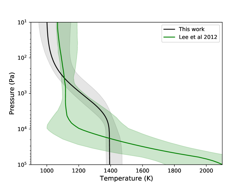
In addition to abundances, Lee et al. (2012) also retrieved a T/P profile (their Figure 1), which we compare to our T/P profile in Figure 13. Although the two profiles are very discrepant at higher pressures ($>\sim$1 bar), it is important to note that constraints on the T/P profile at pressures higher than 1 bar are imposed by the finite range of shapes allowed by the T/P profile parameterization, not by observational data. This is because emission spectroscopy cannot probe those depths, as shown by the contribution function (Figure 10). At low pressures the two profiles are consistent, despite the different shapes.

5.4. Importance of individual molecules

PLATON calculates the abundances and line opacities of 28 molecules. To ascertain which molecules are important, we re-calculate the best fit transit and eclipse spectra with the opacities of individual molecules zeroed out to see how ${\chi}^{2}$ changes. We find that the transit spectrum is dominated by opacity from H₂O, CO₂, H₂S, and CH₄. Removing all other molecular opacities only increases $\chi^{2}$ by 0.7. Starting from a reference point consisting of these four molecules, we remove each molecule in turn and calculate the resulting $\Delta\chi^{2}$, obtaining 1.4 for H₂S, 2.9 for CO₂, 3.6 for CH₄, and 92.9 for H₂O. Zeroing the aerosol opacity yields $\Delta\chi^{2}=3780$. We conclude that water is by far the dominant molecule shaping the transit spectrum, with aerosol scattering as the most important opacity source overall. This is no surprise, as both the strong scattering slope at short wavelengths and the water feature in the WFC3 bandpass are obvious by eye (Figure 7).

The eclipse spectrum worsens by only $\Delta\chi^{2}=0.6$ when the opacity is zeroed for all molecules except H₂O, CO₂, H₂S, CH₄, and CO. Starting from a reference point consisting of these five molecules, we remove each molecule in turn and calculate the resulting $\Delta\chi^{2}$, obtaining 0.2 for CH₄, 8.5 for H₂S, 56.6 for CO, 81.4 for CO₂, and 551 for H₂O. Thus, we conclude that the emission spectrum contains information on more molecules than the transit spectrum, with H₂S, CO, CO₂, and H₂O all acting as important opacity sources, although water is still dominant.

The tests above reveal the contribution of different molecules to the best-fit transit and eclipse spectra. They do not reveal the significance with which individual molecules are detected in the fits, because many of the features induced by a molecule–a little more absorption here, a little less absorption there–can be mimicked by changes in the free parameters. To quantify the detection significance, we ran a series of retrievals on the transit and eclipse data where we zeroed out the opacity of one molecule at a time and calculated the resulting Bayesian evidence $z$. The log of the Bayes ratio (indicating the relative preference for the full model versus one without that molecule) is then given by the difference in $\ln(z)$ when compared to the retrieval where all molecular opacities were included. In transit, $\Delta\ln(z)$ was -0.9 for H₂S, 0.5 for CH₄, -0.8 for CO₂, and -9.9 for H₂O, with a margin of error on $\ln(z)$ equal to $\sim$0.2 for all retrievals. We conclude that the transit spectra only provide strong evidence for H₂O, with a Bayes factor of 20,000; all other molecules have a Bayes factor less than 3. In eclipse, $\Delta\ln(z)$ was 0.3 for H₂S, -0.7 for CO, -1.2 for H₂O, and -1.6 for CO₂, with a similar margin of error. We conclude that the eclipse spectrum does not strongly favor the existence of any one molecule. These results are consistent with intuition: there is a visually obvious water feature in the WFC3 transit spectrum, but no molecular features can be seen in the eclipse spectrum (which is predominately composed of broadband photometric points) at any wavelength.

5.5. Aerosol properties

Many authors have proposed a Rayleigh scattering haze to explain the optical transmission spectrum of HD 189733b (e.g. Lecavelier Des Etangs et al. 2008; Gibson et al. 2012; Pont et al. 2013), and this is born out by our retrievals. Our posteriors indicate that a clear atmosphere with a zero number density of haze particles is ruled out to much greater than $3\sigma$ significance, and the posterior distribution of particle sizes puts the particles firmly in the Rayleigh regime ($r\lesssim\lambda/10$) for optical wavelengths. In fact, our posterior on the mean particle sizes pushes up against 1 nm, the lower end of the prior–indicating that arbitrarily small particles are allowed by the data. This means that no constraint on the haze composition is possible, as the scattering slope is always $\frac{dR_{p}}{d\log{\lambda}}=-4H$ regardless of composition. The lack of a lower limit on the mean particle size also implies that there is no upper limit on the particle density, as there is a perfect degeneracy between the two variables in the Rayleigh regime.

Our findings are consistent with the conclusions of previous studies (i.e. Gibson et al. 2012; Pont et al. 2013), which required the inclusion of a Rayleigh scattering haze in order to reproduce HD 189733b’s infrared transmission spectrum.

Figure 14.— Extinction cross section of the haze particles in our best fit model (solid red), along with the 1$\sigma$ range of extinction cross sections from our retrieval. The dashed solid line falls off as $\lambda^{-4}$, and is plotted for reference.

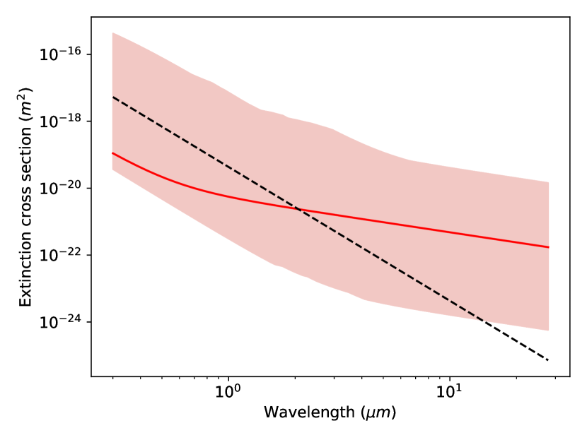
In Figure 14, we show that the aerosol extinction cross section falls as $\lambda^{-4}$ at very short wavelengths, but shifts to $\lambda^{-1}$ at longer wavelengths. This slow dropoff of extinction cross section at high wavelengths is due to aerosol absorption. To understand this, we can write down simple analytic expressions for scattering and absorption cross sections as a function of wavelength in the Rayleigh regime. These are (Mishchenko et al., 2002):

$$\sigma_{sca} =\frac{2^{7}\pi^{5}r^{6}}{3\lambda^{4}}\left\lvert\frac{m^{2}-1}{m^{2}+2}\right\rvert^{2}$$ (15)

$$\sigma_{abs} =\frac{8\pi^{2}r^{3}}{\lambda}Im\Big{(}\frac{m^{2}-1}{m^{2}+2}\Big{)}$$ (16)

Writing the complex refractive index $m$ as $n$ + i$k$, and assuming $k<<n$:

$$\sigma_{sca} =\frac{2^{7}\pi^{5}r^{6}}{3\lambda^{4}}\frac{4k^{2}n^{2}+(n^{2}-k^{2}-1)^{2}}{4k^{2}n^{2}+(n^{2}-k^{2}+2)^{2}}$$

$$\approx\frac{2^{7}\pi^{5}r^{6}}{3\lambda^{4}}\frac{(n^{2}-1)^{2}}{(n^{2}+2)^{2}}$$

$$\sigma_{abs} =\frac{8\pi^{2}r^{3}}{\lambda}\frac{6nk}{(n^{2}-k^{2}+2)^{2}+4k^{2}n^{2}}$$

$$\approx\frac{8\pi^{2}r^{3}}{\lambda}\frac{6nk}{(n^{2}+2)^{2}}$$

One can see from these equations that aerosol scattering falls off with wavelength much faster than aerosol absorption, causing extinction to be dominated by scattering at short wavelengths and absorption at long wavelengths. Since the absorption cross section is proportional to the imaginary component of the refractive index, even a small imaginary component increases long wavelength extinction by orders of magnitude compared to a real refractive index.

The importance of $k$, the imaginary component of the refractive index, poses a challenge for our model. Many different cloud species have been proposed for this planet. Lee et al. (2016) used a GCM simulation to model condensate clouds and found that the clouds are dominated by silicate materials such as MgSiO₃ at mid-high latitudes, but TiO₂ and SiO₂ dominate in equatorial regions. Lavvas & Koskinen (2017) considered photochemical hazes and found that soot-composition aerosols provided a good match to HD 189733b’s transmission spectrum. This study reported $k\sim$ 0.5 at 500 nm for soot, while Kitzmann & Heng (2018) reported 3.7$\times 10^{-5}$ for glassy MgSiO₃ at the same wavelength, 5.1$\times 10^{-4}$ for TiO₂, and 1.7$\times 10^{-5}$ for SiO₂. In addition to these species-dependent variations in $k$, the $k$ for each species also varies drastically (and uniquely) with wavelength. For example, $k$ rises from 1$\times 10^{-4}$ to nearly 1 over the wavelength range $2-9$ µm for MgSiO₃, and SiO₂ exhibits a similar behavior before dropping 2 orders of magnitude within 2 µm. In light of these uncertainties, we chose to fit for a wavelength-independent $k$ value rather than fixing it to the theoretical prediction for a given cloud species.

We argued earlier that the presence of aerosol has a negligible effect on HD 189733b’s dayside emission spectrum. We check the validity of this assumption using our best-fit model. We find that when we include the best-fit aerosol model from the transmission spectrum in our calculation of HD 189733b’s dayside emission spectrum the resulting eclipse depth values change less than $\sim$0.1 ppb, with a corresponding change in ${\chi}^{2}$ of only 2$\times 10^{-5}$. This is unsurprising, as the photospheric pressure is lower for transmission spectrum than it is for eclipse spectrum by a factor of $\sqrt{2\pi R/H}\sim 50$ (Fortney, 2005); this is apparent when we compare the transmission spectrum contribution function in Figure 11 to the emission spectrum contribution function in Figure 10. At higher pressures, the mixing ratio of aerosol is lower because our retrievals prefer an aerosol scale height that is greater than the gas scale height. This causes aerosol absorption to be an important source of opacity at low pressures only. We note that the dayside is also expected to be hotter than the terminator, making it less likely that the condensate clouds detected at the terminator would persist in this region. Even if the dayside is in reality partly cloudy, the dayside emission would be dominated by clear regions because they have deeper and hotter photospheres, which emit more radiation.

5.6. Validity of equilibrium chemistry

PLATON assumes equilibrium chemistry. Since chemical reaction timescales decline rapidly with temperature, the colder a planet, the more disequilibrium chemistry matters. HD 189733b lies in a regime where disequilibrium chemistry may be important. Multiple studies have explored disequilibrium chemistry on this planet (Line et al., 2010; Venot et al., 2012; Moses et al., 2013; Agúndez et al., 2014; Blumenthal et al., 2018; Steinrueck et al., 2019). Venot et al. (2012) considered 1D models with both UV photochemistry and vertical mixing, and found negligible differences in the resulting transmission and emission spectra as compared to equilibrium models. Their Figure 10 shows that the disequilibrium-induced brightness temperature discrepancy is at most several Kelvin (less than 1%), while the transit radius discrepancy is at most $\sim$30 ppm. Blumenthal et al. (2018) also model the emission spectrum under equilibrium and non-equilibrium conditions, finding no detectable difference even with JWST (their Figure 3). Other studies report changes in abundance as a result of disequilibrium chemistry, but do not compare the resulting spectra to the equilibrium model predictions. For example, Moses et al. (2013) find that the water abundance only becomes discrepant for P $<$ 1 microbar, while the HCN abundance is enhanced by orders of magnitude for P $<$0.5 bar. In contrast to these 1D models, which predict relatively small changes in HD 189733b’s observed transmission and emission spectrum, Steinrueck et al. (2019) calculated emission spectra for HD 189733b using general circulation models where they fixed the ratio of CH₄ to CO across the planet to mimic the effect of transport-induced quenching. They find that disequilibrium chemistry due to horizontal transport changes the emission spectrum by up to 20% for a heavily CO-dominated atmosphere (CH₄/CO = 0.001): there is a systematic offset of 10% in addition to wavelength-dependent discrepancies of order several percent.

To test whether disequilibrium chemistry may be important for our data, we performed retrievals on the transit and eclipse spectra with the vertical quench pressure as a free parameter. We quenched all molecules in our first trial, but only CH4 and CO in our second trial (in accordance with Morley et al. 2017), with no change in the following conclusions. Quenching did not result in a better fit ($\Delta\chi^{2}\sim 0$) for either our transmission or emission spectra. In both cases, the posterior distribution of the quench pressure pushes up against the lower bound of the prior–0.1 mbar for the transit spectrum and 1 mbar for the eclipse spectrum. Additionally, the posterior distributions of the other parameters did not appreciably change in these retrievals. For example, the metallicity posterior shifted by 0.1$\sigma$ for the transit retrieval and 0.5$\sigma$ for the eclipse retrieval; the C/O ratio posterior shifted by 0.06$\sigma$ for both transit and eclipse retrievals. We conclude that the effects of disequilibrium chemistry are below our detection threshold, in good agreement with the predictions of the 1D models from Venot et al. (2012) and Blumenthal et al. (2018).

5.7. The effect of starspots

HD 189733 is an active K dwarf with spots that cover a few percent of its surface. When the planet crosses a prominent spot it creates a readily identifiable deviation in the transit light curve shape; this makes it straightforward to identify and mask such events in high signal-to-noise HST observations (e.g. Sing et al., 2011; Pont et al., 2013). However, the presence of unocculted spots during a transit also biases the retrieved transit depth in a way that can mimic the effect of scattering as discussed in McCullough et al. (2014). If the fractional spot coverage varies from one transit epoch to another, the relative effect on the transit depth will vary as well. An additional complication is faculae, bright regions $\sim$100 K hotter than their surroundings. For a K1.5 star like HD 189733, faculae can cover 17-40% of the surface, partially cancelling the effect due to spots (Rackham et al., 2019). The large faculae fraction is a mixed blessing. On one hand, it becomes hard to correct for the effects of faculae because we cannot assume faculae are unocculted. On the other hand, the faculae covering fraction is so large that the planet is likely to cross at least one faculae and one non-faculae region during every transit, thus mitigating the spectral bias from unocculted faculae. We therefore neglect the effects of faculae and only consider spots.

Pont et al. (2013) attempted to correct for the effects of time-varying spot coverage by using photometric data from the Automated Patrol Telescopes (Henry, 1999) to estimate the apparent brightness at the epoch of each transit observation. Although these data made it possible to estimate the magnitude of the variations in spot coverage, they do not provide an estimate of the overall spot coverage fraction because the star is not necessarily spotless at maximum brightness. The authors resolve this problem by assuming an average spot coverage fraction of 1%, based on three pieces of evidence: the frequency of spot-crossing events during HST transits (Sing et al., 2011), stochastic starspot simulations by Aigrain et al. (2012), and the lack of features in the transmission spectrum (i.e. Mg H line, stellar sodium line) caused by abundant starspots. They argue that these lines of evidence make it unlikely that the spot coverage fraction is much above 2%.

McCullough et al. (2014) use the same data to argue for a higher starspot fraction of 4%. First, they emphasize that the starspot fraction derived from spot crossing events would be an underestimate if most starspots are in the polar regions, where the planet does not transit. Second, they use Equation 14 of Aigrain et al. (2012) to derive a lower bound on the starspot fraction:

$$\delta>\approx\frac{\Psi_{max}-\Psi_{min}+\sigma}{\Psi_{max}+\sigma}$$

Since the measured difference between the maximum flux ($\Psi_{max}$) and minimum flux ($\Psi_{min}$) is around 4% and the rotational modulation ($\sigma$) is of order one percent, $\delta>\approx 0.04$. However, this derivation really computes a lower bound on the maximum starspot fraction over a period of time, whereas the 1-2% figure quoted by Pont et al. (2013) is the average starspot fraction. McCullough et al. (2014) go on to argue that if the starspot fraction were 4.3%, the majority of the increased apparent transit depth in the UV compared to IR could be explained by unocculted starspots, and there would be no need to invoke scattering from aerosol.

To shed light on this issue, we ran another retrieval with PLATON where the spot coverage fraction is allowed to vary as a free parameter. We fix the spot temperature to 4250 K, the temperature derived by Sing et al. (2011) from observations of spot occultations. Since we used the transit depths from Pont et al. (2013), which already corrected for the effects of starspots using APT photometry and an assumed 1% baseline starspot fraction, our fitted spot coverage fraction is in reality an excess spot fraction above this 1% baseline. We find an excess spot coverage fraction of $1.8_{-1}^{+0.7}$%, which in turn implies a total average starspot fraction of $2.8_{-1}^{+0.7}$%. This figure is intermediate between the 1-2% argued for by Pont et al. (2013) and the 4% argued by McCullough et al. (2014). However, the inclusion of spot coverage fraction as a free parameter does little to modify the posteriors for the other model parameters. The median values of all parameters are consistent with the values from the fiducial retrieval (Table 6) to better than 1$\sigma$. We therefore conclude that our derived haze properties, including the mean particle size, particle number density, and fractional scale height, are insensitive to our assumptions about the spot coverage fraction.

Figure 15.— PLATON model of a hazy atmosphere on HD 189733b, compared to a clear atmosphere with a starspot-induced slope corresponding to a spot coverage fraction of 6%. Note the strong atomic and molecular features in the clear atmosphere, especially the far wings of the sodium and potassium absorption lines.

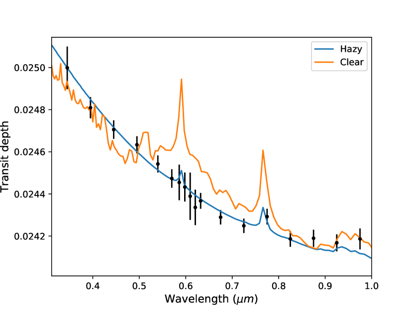
If unocculted starspots and haze can both introduce a slope in HD 189733b’s optical transmission spectrum, why is there not a degeneracy between the two? To answer this question, we plotted a transmission spectrum with no aerosol but with a high spot coverage fraction of 6%, as shown in Figure 15. We found that the transmission spectrum has strong atomic and molecular absorption features even at short wavelengths ($\lambda<1$ µm), the most prominent of which are the far wings of the Na doublet at 589 nm and of the K doublet at 770 nm. These features are not seen in the observational data, which are nearly featureless at optical wavelengths.

5.8. A consistency check for composition

Figure 16.— Posterior distributions for the transit-only retrieval (blue), eclipse-only retrieval (red), and combined retrieval (black).

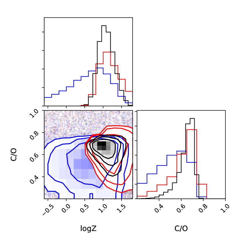
Although we fit HD 189733b’s transmission and emission spectra jointly, in reality the models used to fit these two spectra are largely independent of each other. The transmission spectrum determines the isothermal limb temperature and aerosol properties, while the emission spectrum sets the dayside T/P profile. The planetary radius is technically constrained by both transmission and emission spectra, but most of the statistical power comes from the transmission spectrum. The only two parameters that are comparably constrained by both spectra are the atmospheric metallicity and C/O ratio, which determine the chemistry for both the limb and the day side.

To illustrate the relative contributions of transmission and emission spectra to HD 189733b’s inferred atmospheric composition, we ran a transit-only and an eclipse-only retrieval. In the transit-only retrieval, the planetary radius, metallicity, C/O ratio, isothermal limb temperature, aerosol properties, and WFC3 offset were free parameters. In the eclipse-only retrieval, the metallicity, C/O ratio, dayside T/P profile parameters, and WFC3 offset were free parameters. Figure 16 shows the resulting posterior distributions for metallicity and C/O from these two retrievals, with the distributions from the combined retrieval overplotted. The three retrievals give fully consistent constraints on both parameters. The emission spectrum puts a slightly tighter constraint on metallicity, but both spectra place comparable constraints on the C/O ratio.

5.9. High resolution studies

HD 189733b has been a favorite target for high resolution spectroscopy. VLT/CRIRES detected water on its dayside (Birkby et al., 2013), as well as both water and CO on its terminator (Brogi et al., 2016). TNG/GIANO and CARMENES also detected water in the transit spectrum (Brogi et al., 2018; Alonso-Floriano et al., 2019). Carbon monoxide has been detected on its dayside by both Keck/NIRSPEC (Rodler et al., 2013) and VLT/CRIRES (de Kok et al., 2013). The dayside detections with CRIRES were confirmed by Cabot et al. (2019), who additionally report a high confidence (5.0$\sigma$) detection of HCN, with a HCN mixing ratio of $10^{-6}$ yielding peak detection significance.

We test the robustness of the water and HCN detections with PLATON. We replicate the methodology in Cabot et al. (2019) to reduce the CRIRES L band (3.18–3.27 µm) data. We then generate a high-resolution PLATON model of HD 189733b assuming the best fit parameters to the low resolution data, with only the line opacity of the molecule in question included. The model eclipse spectrum is cross correlated with the data to look for a signal with the expected radial velocity drift of the planet. We detect H₂O and HCN at a significance of 4.3$\sigma$ and 4.8$\sigma$ respectively, in line with the results of Cabot et al. (2019). These results are shown in Figure 17.

While both molecular detections seem robust, they may not be. Standard high resolution analysis methods involve optimizing many parameters to maximize the detection significance. For Cabot et al. (2019), these are the number of SYSREM (principal component analysis to remove telluric features) iterations for each of the 4 detectors, the planetary orbital velocity, the systemic velocity offset, the percentage of wavelengths to mask due to low atmospheric transmission, and the percentage of wavelengths to mask due to high variability. They report from injection-recovery tests that this optimization procedure yields false positives as high as 4.0$\sigma$ 30% of the time.

To reduce the bias introduced by the optimization procedure, we fix the orbital velocity to 152.5 km/s (Brogi et al., 2016) and restrict the systemic velocity offset to $\pm 1$ km/s. We then estimate the bias introduced by the optimization process by a bootstrap-inspired procedure. We randomly select, with replacement, 48 spectra from the original list of 48 spectra to form a new list of 48 spectra in random order. We then apply the same analysis used for the original set of spectra to the new set. This random selection and ordering, combined with the radial acceleration of the planet (amounting to 2 pixels/spectrum), means that the lines in the template will rarely match up with the planetary absorption lines. We expect that the detection significance of all molecules in this scenario should be $0\sigma$, and the magnitude of the recovered signals therefore allows us to estimate the bias introduced by the optimization steps.

We run this bootstrap procedure 1000 times, gathering the “detection significance” from each run. We find that our optimization procedure, despite exploring fewer free parameters than Cabot et al. (2019), returns an average bias of 1.1$\sigma$ for water and 2.9$\sigma$ for HCN. Returning to the original analysis, our bias-corrected detection significance is then 3.2$\sigma$ for water, and 1.9$\sigma$ for HCN. We conclude that the water detection is statistically significant, but the HCN detection is not.

In order to reduce the magnitude of this bias, we modified our analysis to minimize the size of the parameter space we optimize over. Instead of optimizing the two masking parameters, we fix them to reasonable values: we mask wavelengths where the atmospheric transmission is under 30%, and where the standard deviation of the wavelength across all spectra is in the top 10% of all standard deviations for that detector. Instead of optimizing over the four-dimensional space consisting of the number of SYSREM iterations for each detector, we optimize the number of iterations for each detector in turn before summing their weighted CCFs. In addition, we include data from all detectors, instead of excluding the second detector due to the strong telluric absorption at those wavelengths.

These changes turn a 6 dimensional optimization problem into four 1-dimensional optimization problems, each of which can have one of 10 discrete values, drastically decreasing the potential for bias. We also apply a fourth order Butter high-pass filter to both the template and the data with a cutoff frequency of 0.01 pixel^-1, further reducing the potential for low-frequency systematics to create false signals. These simplifications have the additional benefit of making our optimization code much faster. In this new analysis, we find that water is detected at 3.8$\sigma$ with an optimization bias of 0.7$\sigma$ from bootstrapping, resulting in a corrected significance of 3.1$\sigma$. HCN is detected at 2.8$\sigma$ with an optimization bias of 1.3$\sigma$, with a corrected significance of 1.5$\sigma$. These results are in good agreement with our previous conclusions: the water detection is secure, but the HCN detection is statistically insignificant.

Why does our HCN measurement consistently exhibit higher levels of bias than water? Although a detailed investigation of this question is outside the scope of this paper, we offer some speculations based on the differing statistical properties of the water and HCN line lists. Water has a large number of weak lines irregularly spaced across the band, while HCN has a smaller number of very strong lines with a regular periodic spacing. Thus, for HCN, the cross correlation function is dominated by strong lines spanning a smaller number of pixels, making overfitting more likely. The cross correlation function for water depends on contributions from many pixels, making it more difficult to overfit.

The periodic nature of the HCN lines means that the same problem occurs in Fourier space as in wavelength space. Cross correlation is mathematically equivalent to taking the Fourier transform of the template, multiplying it by the conjugate of the Fourier transform of the data, and inverse Fourier transforming the product. For templates with more periodic features, the Fourier transform of the template is dominated by a few high peaks. These peaks may by chance coincide with unsubtracted periodic systematics, resulting in a spurious signal. The Fourier transform for the water template is more evenly distributed, and is therefore less prone to this problem.

There are also physical reasons to doubt the HCN detection. The detections of H₂O and CO are fully consistent with our best fit model to the low resolution data, which predicts that these molecules should be the most abundant active gases in the atmosphere at pressures lower than 1 bar. These same models predict that the spectral signature of HCN should be significantly weaker than the signals from the more abundant H₂O and CH₄. CH₄ has a slightly higher absorption cross section between $3.18-3.27$ µm, the wavelength range CRIRES covers. While H₂O has a lower cross section over these wavelengths, it is many orders of magnitude more abundant. Therefore, we would not expect HCN to be observable unless its abundance exceeds that of methane and is at least $\sim$10% that of water; this would be many orders of magnitudes higher than predictions from equilibrium chemistry models for this planet.

One way around this difficulty is to invoke disequilibrium chemistry, as HCN abundances are enhanced both by transport-induced quenching and by photochemistry. Moses et al. (2011) simulated HD 189733b and found that its HCN abundance is enhanced by disequilibrium processes. Encouragingly, they found HCN abundances close to $10^{-5}$, similar to the $10^{-6}$ inferred observationally by Cabot et al. (2019). However, they find that CH₄ abundances are enhanced by the same processes, leaving the CH₄ abundance greater than or similar to the HCN abundance at typical photospheric pressures of 100 mbar. They also find that the water abundance is not changed except at very high altitudes.

The dominance of CH₄ in the models raises the question of whether the high-resolution CRIRES data shows any evidence of CH₄. We searched for methane using the same CRIRES data by utilizing the methane line list by Rey et al. (2017), which is complete at these high temperatures and has accurate line positions suitable for high resolution studies. We find only a 1.2$\sigma$ signal, which is not significant. This result is shown in Figure 17.

Figure 17.— Detection significance of H₂O, HCN, and CH₄ in the high resolution emission spectrum of HD 189733b. H₂O and HCN are seemingly clearly detected, while CH₄ is not. The model used to cross correlate with data was generated by PLATON using the parameters of the best fit model from the low resolution retrieval. Despite the seeming robustness of the HCN detection, bootstrap analysis reveals that its actual significance is 1.5–1.9$\sigma$.

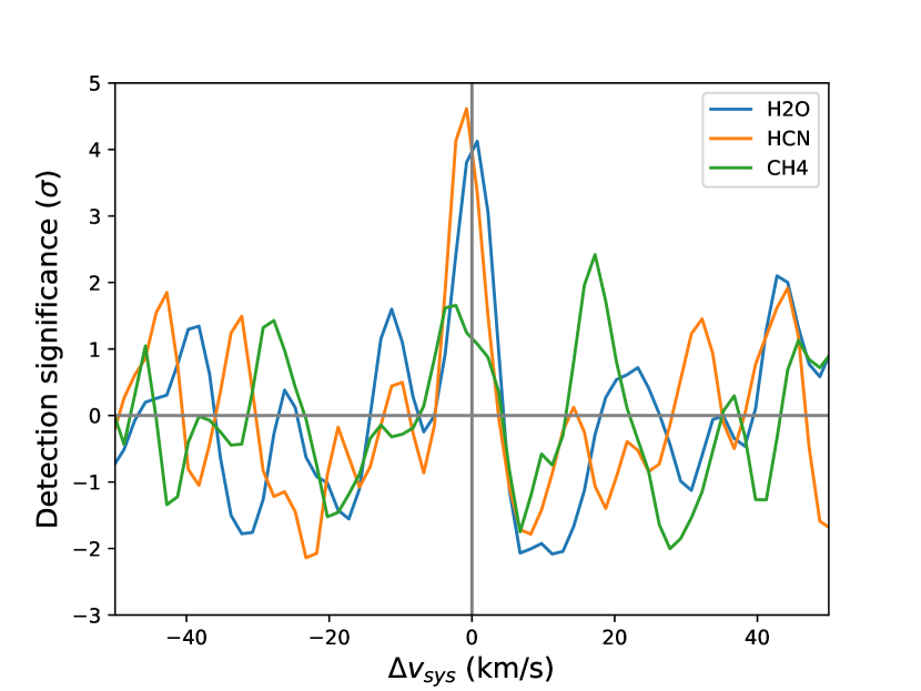
6. Conclusion

A new and improved PLATON is available for download.. It now comes with an eclipse depth calculator, updated opacities, joint transit-eclipse retrieval capability, and correlated-$k$ capability. In addition, we provide high resolution opacity data, making line-by-line calculations possible for the first time. We demonstrate PLATON’s new capabilities by using it to simultaneously analyze the best available HST and Spitzer transit and eclipse depths for the archetypal hot Jupiter HD 189733b. To our knowledge, this is the first published retrieval on this comprehensive data set, as well as the first published joint retrieval that includes both transmission and emission spectroscopy.

Our resulting inferences for the properties of HD 189733b’s atmosphere are qualitatively similar to–but more constraining than–those of previous authors. We find that the data favors a haze with a mean particle radius less than 14 nm. Our fiducial T/P profile indicates that the planet is consistent with a zero-albedo object with perfect heat redistribution. We find that the atmosphere is of moderately super-solar ($7-21\times$ solar) metallicity and constrain the C/O ratio to lie between $0.47-0.69$, consistent with the solar value, but possibly lower than the stellar value. This planet has one of the tightest metallicity constraints ever measured, with only WASP-127b and WASP-39b being comparable (see Figure 22 of Spake et al. 2019). In our best-fit model, CO and H₂O are the most abundant absorbing species at photospheric pressures, consistent with the detection of H₂O in HST/WFC3 spectroscopy, and the detection of both molecules in high resolution spectroscopy.

We explore the effects of stellar activity using a retrieval in which the starspot coverage fraction is allowed to vary as a free parameter, and find a best-fit starspot coverage fraction of $1.8_{-1}^{+0.7}$%. Even when this coverage is allowed to vary, our fit still requires the presence of a haze with much the same properties as the fiducial retrieval in order to create a featureless optical transit spectrum.

HD 189733b has exceptional observational data unmatched by any other exoplanet in quality, quantity, or wavelength range. Much of this data was collected by Spitzer or by now-defunct instruments on HST, and can never be replicated. Our retrieval demonstrates what kinds of properties can be inferred, and to what precision, for the most observationally favorable hot Jupiters in the pre-JWST era. We have come close to testing the prediction by Espinoza et al. (2017) that enhanced atmospheric metallicity is inevitably associated with sub-stellar C/O ratio–in fact, the main obstacle was the uncertain stellar C/O ratio. In addition, although the data for HD 189733b are already far more accurate than our models–the 3.6, 4.5, and 8.0 eclipse depths have errors of 1-2%, whereas we have demonstrated that small changes in PLATON’s (and TauREx’s) algorithm change the eclipse depth by several percent–we cannot fully take advantage of this accuracy in a retrieval. This is because a retrieval has enough free parameters to fit the 3.6, 4.5, and 8.0 eclipse depths to arbitrary accuracy, and the lack of any molecular features in emission contributes to wide posteriors on atmospheric parameters despite the exceptional data. JWST will be able to accurately measure multiple emission bands from multiple molecules across a large wavelength range, spurring spur the development of more sophisticated and more accurate models than the current state of the art.

7. Acknowledgments

M.Z. acknowledges Plato (Greek:$\Pi\Lambda\mathrm{AT}\Omega\mathrm{N}$) for his clear and thought-provoking dialogues, which ought to be exemplars of good writing for academics everywhere. We also thank Michael R. Line for helpful advice. Support for this work was provided by HST GO programs 13431, 13665, and 14260.

Software: numpy (van der Walt et al., 2011), scipy (Virtanen et al., 2020), matplotlib (Hunter, 2007), emcee (Foreman-Mackey et al., 2013), dynesty (Speagle, 2020), corner (Foreman-Mackey, 2016), nose, Travis-CI

8. Appendix

The following HD 189733b parameters in Table 7 were fixed during the retrieval:

Table 7Fixed planetary parameters in HD 189733b retrieval

Parameter	Value
$T_{s}$	5052 K
$R_{s}$	0.751 $R_{\odot}$
$M_{p}$	1.129 $M_{J}$
a	0.03142 AU

Tables 8 and 9 list the transit and eclipse depths we used in the retrieval, along with the papers they were taken from.

Table 8Adopted transit depths. Sources: (1) Pont et al. 2013; (2) McCullough et al. 2014

$\lambda_{min}$(µm)	$\lambda_{max}$(µm)	Depth (ppm)	Error (ppm)	Source
$0.32$	$0.37$	$24999$	$101$	$1$
$0.37$	$0.42$	$24809$	$50$	$1$
$0.42$	$0.47$	$24706$	$44$	$1$
$0.47$	$0.52$	$24633$	$41$	$1$
$0.52$	$0.56$	$24542$	$41$	$1$
$0.56$	$0.58$	$24473$	$44$	$1$
$0.58$	$0.592$	$24455$	$84$	$1$
$0.592$	$0.604$	$24433$	$69$	$1$
$0.604$	$0.615$	$24389$	$112$	$1$
$0.615$	$0.626$	$24336$	$84$	$1$
$0.626$	$0.638$	$24367$	$37$	$1$
$0.65$	$0.7$	$24289$	$34$	$1$
$0.7$	$0.75$	$24249$	$34$	$1$
$0.75$	$0.8$	$24292$	$37$	$1$
$0.8$	$0.85$	$24186$	$37$	$1$
$0.85$	$0.9$	$24190$	$40$	$1$
$0.9$	$0.95$	$24168$	$40$	$1$
$0.95$	$1.0$	$24186$	$50$	$1$
$1.0$	$1.17$	$24062$	$68$	$1$
$1.1184$	$1.1374$	$23962$	$73$	$2$
$1.1372$	$1.1562$	$24047$	$67$	$2$
$1.156$	$1.175$	$24078$	$105$	$2$
$1.1748$	$1.1938$	$24035$	$87$	$2$
$1.1936$	$1.2126$	$23961$	$80$	$2$
$1.2123$	$1.2313$	$23955$	$70$	$2$
$1.2311$	$1.2501$	$23884$	$56$	$2$
$1.2499$	$1.2689$	$24000$	$62$	$2$
$1.2687$	$1.2877$	$23863$	$61$	$2$
$1.2875$	$1.3065$	$23987$	$69$	$2$
$1.3062$	$1.3252$	$23961$	$60$	$2$
$1.325$	$1.344$	$23982$	$66$	$2$
$1.3438$	$1.3628$	$24134$	$55$	$2$
$1.3626$	$1.3816$	$24149$	$61$	$2$
$1.3814$	$1.4004$	$24091$	$63$	$2$
$1.4001$	$1.4191$	$24215$	$77$	$2$
$1.4189$	$1.4379$	$24199$	$64$	$2$
$1.4377$	$1.4567$	$24108$	$71$	$2$
$1.4565$	$1.4755$	$24018$	$67$	$2$
$1.4752$	$1.4942$	$24188$	$75$	$2$
$1.494$	$1.513$	$23941$	$62$	$2$
$1.5128$	$1.5318$	$24097$	$61$	$2$
$1.5316$	$1.5506$	$24002$	$62$	$2$
$1.5504$	$1.5694$	$24010$	$72$	$2$
$1.5691$	$1.5881$	$24100$	$87$	$2$
$1.5879$	$1.6069$	$23963$	$75$	$2$
$1.6067$	$1.6257$	$23916$	$98$	$2$
$1.6255$	$1.6445$	$24062$	$84$	$2$
$3.2$	$3.9$	$24047$	$84$	$1$
$4.0$	$5.0$	$24155$	$109$	$1$
$5.0$	$6.4$	$23951$	$207$	$1$
$6.4$	$9.3$	$24056$	$105$	$1$
$23.5$	$24.5$	$23898$	$291$	$1$

Table 9Adopted eclipse depths. Sources: (1) Crouzet et al. 2014; (2) Kilpatrick et al. 2020; (3) Charbonneau et al. 2008; (4) Agol et al. 2010

$\lambda_{min}$(µm)	$\lambda_{max}$(µm)	Depth (ppm)	Error (ppm)	Source
$1.1184$	$1.1374$	$0$	$47$	$1$
$1.1372$	$1.1562$	$78$	$50$	$1$
$1.156$	$1.175$	$124$	$45$	$1$
$1.1748$	$1.1938$	$93$	$44$	$1$
$1.1936$	$1.2126$	$89$	$43$	$1$
$1.2123$	$1.2313$	$51$	$50$	$1$
$1.2311$	$1.2501$	$64$	$42$	$1$
$1.2499$	$1.2689$	$99$	$42$	$1$
$1.2687$	$1.2877$	$80$	$42$	$1$
$1.2874$	$1.3064$	$149$	$41$	$1$
$1.3062$	$1.3252$	$127$	$41$	$1$
$1.325$	$1.344$	$108$	$41$	$1$
$1.3438$	$1.3628$	$75$	$41$	$1$
$1.3626$	$1.3816$	$69$	$41$	$1$
$1.3813$	$1.4003$	$56$	$42$	$1$
$1.4001$	$1.4191$	$104$	$42$	$1$
$1.4189$	$1.4379$	$94$	$42$	$1$
$1.4377$	$1.4567$	$67$	$42$	$1$
$1.4565$	$1.4755$	$32$	$43$	$1$
$1.4753$	$1.4943$	$105$	$43$	$1$
$1.494$	$1.513$	$228$	$43$	$1$
$1.5128$	$1.5318$	$211$	$43$	$1$
$1.5316$	$1.5506$	$143$	$44$	$1$
$1.5504$	$1.5694$	$99$	$45$	$1$
$1.5691$	$1.5881$	$135$	$45$	$1$
$1.5879$	$1.6069$	$80$	$46$	$1$
$1.6067$	$1.6257$	$32$	$46$	$1$
$1.6255$	$1.6445$	$110$	$74$	$1$
$3.2$	$4.0$	$1481$	$34$	$2$
$4.0$	$5.0$	$1827$	$22$	$2$
$5.1$	$6.3$	$3100$	$340$	$3$
$6.6$	$9.0$	$3440$	$36$	$4$
$13.5$	$18.5$	$5190$	$220$	$3$
$20.8$	$26.1$	$5980$	$380$	$3$

Table 10ExoMol line lists used in PLATON v5

Molecule	List name	Nlines	Tmax(K)	Reference
C2H4	MaYTY	49,673,223,799*	700	Mant et al. (2018)
CO	Li2015	125,496*	9000	Li et al. (2015)
H2CO	AYTY	12,648,694,479*	1500*	Al-Refaie et al. (2015)
H2S	AYT2	115,623,180*	2000*	Azzam et al. (2016)
H2O	POKAZATEL	5,550,587,708*	$\infty^{b}$*	Polyansky et al. (2018)
HCl	Yueqi	2588	?	Li et al. (2013)
HCN	Harris	34,418,408*	?	Barber et al. (2013)
MgH	MoLLIST	14,179*	?	GharibNezhad et al. (2013)
NH3	CoYuTe	1,135,240,003*	1500*	Coles et al. (2019)
NO	NOname	2,280,366*	?	Wong et al. (2017)
OH	MoLLIST	54,276	?	Brooke et al. (2016)
PH3	SAlTY	16,931,647,841*	1500*	Sousa-Silva et al. (2014)
SH	SNaSH	81,348*	5000	Yurchenko et al. (2018)
SiH	SiGHTLY	1,724,841*	5000	Yurchenko et al. (2017)
SiO	EBJT	254,675*	9000	Barton et al. (2013)
SO2	ExoAmes	1,402,257,689*	2000	Underwood et al. (2016)
TiO	ToTo	295,086,011a	5000	McKemmish et al. (2019)
VO	VOMYT	277,131,624	5000	McKemmish et al. (2016)

References

- Agol et al. (2010) Agol, E., Cowan, N. B., Knutson, H. A., et al. 2010, ApJ, 721, 1861
- Agúndez et al. (2014) Agúndez, M., Parmentier, V., Venot, O., Hersant, F., & Selsis, F. 2014, A&A, 564, A73
- Agúndez et al. (2012) Agúndez, M., Venot, O., Iro, N., et al. 2012, A&A, 548, A73
- Aigrain et al. (2012) Aigrain, S., Pont, F., & Zucker, S. 2012, MNRAS, 419, 3147
- Al-Refaie et al. (2019) Al-Refaie, A. F., Changeat, Q., Waldmann, I. P., & Tinetti, G. 2019, arXiv e-prints, arXiv:1912.07759
- Al-Refaie et al. (2015) Al-Refaie, A. F., Yachmenev, A., Tennyson, J., & Yurchenko, S. N. 2015, Monthly Notices of the Royal Astronomical Society, 448, 1704
- Ali-Dib (2017) Ali-Dib, M. 2017, MNRAS, 467, 2845
- Allard et al. (2012) Allard, F., Homeier, D., & Freytag, B. 2012, Philosophical Transactions of the Royal Society of London Series A, 370, 2765
- Allard et al. (2019) Allard, N. F., Spiegelman, F., Leininger, T., & Molliere, P. 2019, A&A, 628, A120
- Allard, N. F. et al. (2016) Allard, N. F., Spiegelman, F., & Kielkopf, J. F. 2016, A&A, 589, A21
- Alonso-Floriano et al. (2019) Alonso-Floriano, F. J., Sánchez-López, A., Snellen, I. A. G., et al. 2019, A&A, 621, A74
- Amundsen et al. (2017) Amundsen, D. S., Tremblin, P., Manners, J., Baraffe, I., & Mayne, N. J. 2017, A&A, 598, A97
- Azzam et al. (2016) Azzam, A. A. A., Tennyson, J., Yurchenko, S. N., & Naumenko, O. V. 2016, Monthly Notices of the Royal Astronomical Society, 460, 4063
- Barber et al. (2013) Barber, R. J., Strange, J. K., Hill, C., et al. 2013, Monthly Notices of the Royal Astronomical Society, 437, 1828
- Barstow et al. (2014) Barstow, J. K., Aigrain, S., Irwin, P. G. J., et al. 2014, ApJ, 786, 154
- Barton et al. (2017) Barton, E. J., Hill, C., Czurylo, M., et al. 2017, J. Quant. Spec. Radiat. Transf., 203, 490
- Barton et al. (2013) Barton, E. J., Yurchenko, S. N., & Tennyson, J. 2013, Monthly Notices of the Royal Astronomical Society, 434, 1469
- Beaulieu et al. (2008) Beaulieu, J. P., Carey, S., Ribas, I., & Tinetti, G. 2008, ApJ, 677, 1343
- Benneke (2015) Benneke, B. 2015, arXiv e-prints, arXiv:1504.07655
- Birkby (2018) Birkby, J. L. 2018, arXiv e-prints, arXiv:1806.04617
- Birkby et al. (2013) Birkby, J. L., de Kok, R. J., Brogi, M., et al. 2013, MNRAS, 436, L35
- Blecic (2016) Blecic, J. 2016, ArXiv e-prints, 1604.02692
- Blecic et al. (2017) Blecic, J., Dobbs-Dixon, I., & Greene, T. 2017, ApJ, 848, 127
- Blecic et al. (2016) Blecic, J., Harrington, J., & Bowman, M. O. 2016, ApJS, 225, 4
- Blumenthal et al. (2018) Blumenthal, S. D., Mandell, A. M., Hébrard, E., et al. 2018, ApJ, 853, 138
- Booth & Ilee (2019) Booth, R. A., & Ilee, J. D. 2019, MNRAS, 487, 3998
- Bouanich et al. (2003) Bouanich, J.-P., Blanquet, G., Walrand, J., & Lepère, M. 2003, Journal of Molecular Spectroscopy, 218, 22
- Bouchy et al. (2005) Bouchy, F., Udry, S., Mayor, M., et al. 2005, A&A, 444, L15
- Brogi et al. (2016) Brogi, M., de Kok, R. J., Albrecht, S., et al. 2016, ApJ, 817, 106
- Brogi et al. (2018) Brogi, M., Giacobbe, P., Guilluy, G., et al. 2018, A&A, 615, A16
- Brogi et al. (2013) Brogi, M., Snellen, I. A. G., de Kok, R. J., et al. 2013, ApJ, 767, 27
- Brooke et al. (2016) Brooke, J. S. A., Bernath, P. F., Western, C. M., et al. 2016, J. Quant. Spec. Radiat. Transf., 168, 142
- Cabot et al. (2019) Cabot, S. H. C., Madhusudhan, N., Hawker, G. A., & Gandhi, S. 2019, MNRAS, 482, 4422
- Chachan et al. (2019) Chachan, Y., Knutson, H. A., Gao, P., et al. 2019, AJ, 158, 244
- Charbonneau et al. (2008) Charbonneau, D., Knutson, H. A., Barman, T., et al. 2008, ApJ, 686, 1341
- Coles et al. (2019) Coles, P. A., Yurchenko, S. N., & Tennyson, J. 2019, Monthly Notices of the Royal Astronomical Society, 490, 4638
- Cridland et al. (2019) Cridland, A. J., van Dishoeck, E. F., Alessi, M., & Pudritz, R. E. 2019, A&A, 632, A63
- Crouzet et al. (2014) Crouzet, N., McCullough, P. R., Deming, D., & Madhusudhan, N. 2014, ApJ, 795, 166
- de Kok et al. (2013) de Kok, R. J., Brogi, M., Snellen, I. A. G., et al. 2013, A&A, 554, A82
- Deming et al. (2006) Deming, D., Harrington, J., Seager, S., & Richardson, L. J. 2006, The Astrophysical Journal, 644, 560
- Deming et al. (2013) Deming, D., Wilkins, A., McCullough, P., et al. 2013, ApJ, 774, 95
- Deming & Seager (2017) Deming, L. D., & Seager, S. 2017, Journal of Geophysical Research (Planets), 122, 53
- Désert et al. (2011) Désert, J. M., Sing, D., Vidal-Madjar, A., et al. 2011, A&A, 526, A12
- Espinoza et al. (2017) Espinoza, N., Fortney, J. J., Miguel, Y., Thorngren, D., & Murray-Clay, R. 2017, The Astrophysical Journal, 838, L9
- Evans et al. (2013) Evans, T. M., Pont, F., Sing, D. K., et al. 2013, ApJ, 772, L16
- Foreman-Mackey (2016) Foreman-Mackey, D. 2016, The Journal of Open Source Software, 1, 24
- Foreman-Mackey et al. (2013) Foreman-Mackey, D., Hogg, D. W., Lang, D., & Goodman, J. 2013, PASP, 125, 306
- Fortney (2005) Fortney, J. J. 2005, Monthly Notices of the Royal Astronomical Society, 364, 649
- Fortney et al. (2019) Fortney, J. J., Lupu, R. E., Morley, C. V., Freedman, R. S., & Hood, C. 2019, The Astrophysical Journal, 880, L16
- Freedman et al. (2014) Freedman, R. S., Lustig-Yaeger, J., Fortney, J. J., et al. 2014, ApJS, 214, 25
- Freedman et al. (2008) Freedman, R. S., Marley, M. S., & Lodders, K. 2008, ApJS, 174, 504
- GharibNezhad et al. (2013) GharibNezhad, E., Shayesteh, A., & Bernath, P. F. 2013, MNRAS, 432, 2043
- Gibson et al. (2011) Gibson, N. P., Pont, F., & Aigrain, S. 2011, MNRAS, 411, 2199
- Gibson et al. (2012) Gibson, N. P., Aigrain, S., Pont, F., et al. 2012, MNRAS, 422, 753
- Goody et al. (1989) Goody, R., West, R., Chen, L., & Crisp, D. 1989, Journal of Quantitative Spectroscopy and Radiative Transfer, 42, 539
- Gordon et al. (2017) Gordon, I. E., Rothman, L. S., Hill, C., et al. 2017, J. Quant. Spec. Radiat. Transf., 203, 3
- Grillmair et al. (2008) Grillmair, C. J., Burrows, A., Charbonneau, D., et al. 2008, Nature, 456, 767
- Grimm & Heng (2015) Grimm, S. L., & Heng, K. 2015, ApJ, 808, 182
- Guillot (2010) Guillot, T. 2010, A&A, 520, A27
- Guo et al. (2020) Guo, X., Crossfield, I. J. M., Dragomir, D., et al. 2020, The Astronomical Journal, 159, 239
- Hayes et al. (2020) Hayes, J. J. C., Kerins, E., Awiphan, S., et al. 2020, MNRAS
- Haynes et al. (2015) Haynes, K., Mandell, A. M., Madhusudhan, N., Deming, D., & Knutson, H. 2015, ApJ, 806, 146
- Hedges & Madhusudhan (2016) Hedges, C., & Madhusudhan, N. 2016, MNRAS, 458, 1427
- Helling et al. (2016) Helling, C., Lee, G., Dobbs-Dixon, I., et al. 2016, MNRAS, 460, 855
- Henry (1999) Henry, G. W. 1999, PASP, 111, 845
- Huitson et al. (2012) Huitson, C. M., Sing, D. K., Vidal-Madjar, A., et al. 2012, MNRAS, 422, 2477
- Hunter (2007) Hunter, J. D. 2007, Computing in Science and Engineering, 9, 90
- John (1988) John, T. L. 1988, A&A, 193, 189
- Karman et al. (2019) Karman, T., Gordon, I. E., van der Avoird, A., et al. 2019, Icarus, 328, 160
- Kempton et al. (2017) Kempton, E. M.-R., Lupu, R., Owusu-Asare, A., Slough, P., & Cale, B. 2017, PASP, 129, 044402
- Kilpatrick et al. (2020) Kilpatrick, B. M., Kataria, T., Lewis, N. K., et al. 2020, AJ, 159, 51
- Kipping & Tinetti (2010) Kipping, D. M., & Tinetti, G. 2010, MNRAS, 407, 2589
- Kirk et al. (2019) Kirk, J., López-Morales, M., Wheatley, P. J., et al. 2019, AJ, 158, 144
- Kitzmann & Heng (2018) Kitzmann, D., & Heng, K. 2018, MNRAS, 475, 94
- Kitzmann et al. (2020) Kitzmann, D., Heng, K., Oreshenko, M., et al. 2020, ApJ, 890, 174
- Knutson et al. (2007) Knutson, H. A., Charbonneau, D., Noyes, R. W., Brown, T. M., & Gilliland, R. L. 2007, ApJ, 655, 564
- Knutson et al. (2009) Knutson, H. A., Charbonneau, D., Cowan, N. B., et al. 2009, ApJ, 690, 822
- Knutson et al. (2012) Knutson, H. A., Lewis, N., Fortney, J. J., et al. 2012, ApJ, 754, 22
- Komacek et al. (2019) Komacek, T. D., Jansen, M. F., Wolf, E. T., & Abbot, D. S. 2019, ApJ, 883, 46
- Kreidberg et al. (2014) Kreidberg, L., Bean, J. L., Désert, J.-M., et al. 2014, ApJ, 793, L27
- Lacis & Oinas (1991) Lacis, A. A., & Oinas, V. 1991, J. Geophys. Res., 96, 9027
- Lavvas & Koskinen (2017) Lavvas, P., & Koskinen, T. 2017, ApJ, 847, 32
- Lecavelier Des Etangs et al. (2008) Lecavelier Des Etangs, A., Pont, F., Vidal-Madjar, A., & Sing, D. 2008, A&A, 481, L83
- Lee et al. (2016) Lee, G., Dobbs-Dixon, I., Helling, C., Bognar, K., & Woitke, P. 2016, A&A, 594, A48
- Lee et al. (2015) Lee, G., Helling, C., Dobbs-Dixon, I., & Juncher, D. 2015, A&A, 580, A12
- Lee et al. (2012) Lee, J. M., Fletcher, L. N., & Irwin, P. G. J. 2012, MNRAS, 420, 170
- Lee et al. (2013) Lee, J.-M., Heng, K., & Irwin, P. G. J. 2013, ApJ, 778, 97
- Lee et al. (2014) Lee, J.-M., Irwin, P. G. J., Fletcher, L. N., Heng, K., & Barstow, J. K. 2014, The Astrophysical Journal, 789, 14
- Li et al. (2015) Li, G., Gordon, I. E., Rothman, L. S., et al. 2015, The Astrophysical Journal Supplement Series, 216, 15
- Li et al. (2013) Li, G., Gordon, I. E., Roy, R. J. L., et al. 2013, Journal of Quantitative Spectroscopy and Radiative Transfer, 121, 78
- Line et al. (2010) Line, M. R., Liang, M. C., & Yung, Y. L. 2010, ApJ, 717, 496
- Line et al. (2013) Line, M. R., Wolf, A. S., Zhang, X., et al. 2013, ApJ, 775, 137
- Line et al. (2016) Line, M. R., Stevenson, K. B., Bean, J., et al. 2016, AJ, 152, 203
- Lines et al. (2018) Lines, S., Mayne, N. J., Boutle, I. A., et al. 2018, A&A, 615, A97
- Lodders (2003) Lodders, K. 2003, ApJ, 591, 1220
- Lupu et al. (2014) Lupu, R. E., Zahnle, K., Marley, M. S., et al. 2014, ApJ, 784, 27
- Madhusudhan (2018) Madhusudhan, N. 2018, Atmospheric Retrieval of Exoplanets (Cham: Springer International Publishing), 2153–2182
- Madhusudhan (2019) —. 2019, Annual Review of Astronomy and Astrophysics, 57, 617
- Madhusudhan et al. (2014) Madhusudhan, N., Knutson, H., Fortney, J. J., & Barman, T. 2014, Protostars and Planets VI, 739
- Madhusudhan & Seager (2009) Madhusudhan, N., & Seager, S. 2009, ApJ, 707, 24
- Mant et al. (2018) Mant, B. P., Yachmenev, A., Tennyson, J., & Yurchenko, S. N. 2018, Monthly Notices of the Royal Astronomical Society, 478, 3220
- Marley & Robinson (2015) Marley, M. S., & Robinson, T. D. 2015, ARA&A, 53, 279
- McCullough et al. (2014) McCullough, P. R., Crouzet, N., Deming, D., & Madhusudhan, N. 2014, ApJ, 791, 55
- McKemmish et al. (2019) McKemmish, L. K., Masseron, T., Hoeijmakers, H. J., et al. 2019, Monthly Notices of the Royal Astronomical Society, 488, 2836
- McKemmish et al. (2016) McKemmish, L. K., Yurchenko, S. N., & Tennyson, J. 2016, Monthly Notices of the Royal Astronomical Society, 463, 771
- Mishchenko et al. (2002) Mishchenko, M. I., Travis, L. D., & Lacis, A. A. 2002, Scattering, absorption, and emission of light by small particles
- Mollière et al. (2019) Mollière, P., Wardenier, J. P., van Boekel, R., et al. 2019, A&A, 627, A67
- Morello et al. (2014) Morello, G., Waldmann, I. P., Tinetti, G., et al. 2014, ApJ, 786, 22
- Morley et al. (2017) Morley, C. V., Knutson, H., Line, M., et al. 2017, AJ, 153, 86
- Moses et al. (2013) Moses, J. I., Madhusudhan, N., Visscher, C., & Freedman, R. S. 2013, ApJ, 763, 25
- Moses et al. (2011) Moses, J. I., Visscher, C., Fortney, J. J., et al. 2011, ApJ, 737, 15
- Ngo et al. (2012) Ngo, N. H., Tran, H., & Gamache, R. R. 2012, J. Chem. Phys., 136, 154310
- Öberg et al. (2011) Öberg, K. I., Murray-Clay, R., & Bergin, E. A. 2011, ApJ, 743, L16
- Ohno & Kawashima (2020) Ohno, K., & Kawashima, Y. 2020, ApJ, 895, L47
- Pinhas et al. (2019) Pinhas, A., Madhusudhan, N., Gandhi, S., & MacDonald, R. 2019, MNRAS, 482, 1485
- Polyansky et al. (2018) Polyansky, O. L., Kyuberis, A. A., Zobov, N. F., et al. 2018, Monthly Notices of the Royal Astronomical Society, 480, 2597
- Pont et al. (2008) Pont, F., Knutson, H., Gilliland, R. L., Moutou, C., & Charbonneau, D. 2008, MNRAS, 385, 109
- Pont et al. (2013) Pont, F., Sing, D. K., Gibson, N. P., et al. 2013, MNRAS, 432, 2917
- Rackham et al. (2019) Rackham, B. V., Apai, D., & Giampapa, M. S. 2019, AJ, 157, 96
- Reuter & Sirota (1993) Reuter, D. C., & Sirota, J. M. 1993, J. Quant. Spec. Radiat. Transf., 50, 477
- Rey et al. (2017) Rey, M., Nikitin, A. V., & Tyuterev, V. G. 2017, ApJ, 847, 105
- Richard et al. (2012) Richard, C., Gordon, I. E., Rothman, L. S., et al. 2012, J. Quant. Spec. Radiat. Transf., 113, 1276
- Rodler et al. (2013) Rodler, F., Kürster, M., & Barnes, J. R. 2013, in European Physical Journal Web of Conferences, Vol. 47, European Physical Journal Web of Conferences, 11003
- Sharp & Burrows (2007) Sharp, C. M., & Burrows, A. 2007, ApJS, 168, 140
- Showman & Polvani (2011) Showman, A. P., & Polvani, L. M. 2011, ApJ, 738, 71
- Shulyak et al. (2019) Shulyak, D., Rengel, M., Reiners, A., Seemann, U., & Yan, F. 2019, A&A, 629, A109
- Sing et al. (2009) Sing, D. K., Désert, J. M., Lecavelier Des Etangs, A., et al. 2009, A&A, 505, 891
- Sing et al. (2011) Sing, D. K., Pont, F., Aigrain, S., et al. 2011, MNRAS, 416, 1443
- Snellen et al. (2010) Snellen, I. A. G., de Kok, R. J., de Mooij, E. J. W., & Albrecht, S. 2010, Nature, 465, 1049
- Sousa-Silva et al. (2014) Sousa-Silva, C., Al-Refaie, A. F., Tennyson, J., & Yurchenko, S. N. 2014, Monthly Notices of the Royal Astronomical Society, 446, 2337
- Southworth (2010) Southworth, J. 2010, MNRAS, 408, 1689
- Spake et al. (2019) Spake, J. J., Sing, D. K., Wakeford, H. R., et al. 2019, arXiv e-prints, arXiv:1911.08859
- Speagle (2020) Speagle, J. S. 2020, Monthly Notices of the Royal Astronomical Society, 493, 3132
- Stassun et al. (2017) Stassun, K. G., Collins, K. A., & Gaudi, B. S. 2017, AJ, 153, 136
- Steinrueck et al. (2019) Steinrueck, M. E., Parmentier, V., Showman, A. P., Lothringer, J. D., & Lupu, R. E. 2019, ApJ, 880, 14
- Stevenson et al. (2010) Stevenson, K. B., Harrington, J., Nymeyer, S., et al. 2010, Nature, 464, 1161
- Swain et al. (2008) Swain, M. R., Vasisht, G., & Tinetti, G. 2008, Nature, 452, 329
- Swain et al. (2009) Swain, M. R., Vasisht, G., Tinetti, G., et al. 2009, ApJ, 690, L114
- Tennyson & Yurchenko (2018) Tennyson, J., & Yurchenko, S. 2018, Atoms, 6, 26
- Teske et al. (2014) Teske, J. K., Cunha, K., Smith, V. V., Schuler, S. C., & Griffith, C. A. 2014, The Astrophysical Journal, 788, 39
- Tinetti et al. (2007) Tinetti, G., Vidal-Madjar, A., Liang, M.-C., et al. 2007, Nature, 448, 169
- Todorov et al. (2014) Todorov, K. O., Deming, D., Burrows, A., & Grillmair, C. J. 2014, ApJ, 796, 100
- Underwood et al. (2016) Underwood, D. S., Tennyson, J., Yurchenko, S. N., et al. 2016, Monthly Notices of the Royal Astronomical Society, 459, 3890
- van der Walt et al. (2011) van der Walt, S., Colbert, S. C., & Varoquaux, G. 2011, Computing in Science and Engineering, 13, 22
- Venot et al. (2012) Venot, O., Hébrard, E., Agúndez, M., et al. 2012, A&A, 546, A43
- Virtanen et al. (2020) Virtanen, P., Gommers, R., Oliphant, T. E., et al. 2020, Nature Methods, 17, 261
- Waldmann et al. (2015) Waldmann, I. P., Rocchetto, M., Tinetti, G., et al. 2015, ApJ, 813, 13
- Woitke et al. (2018) Woitke, P., Helling, C., Hunter, G. H., et al. 2018, A&A, 614, A1
- Wong et al. (2017) Wong, A., Yurchenko, S. N., Bernath, P., et al. 2017, Monthly Notices of the Royal Astronomical Society, 470, 882
- Yurchenko et al. (2018) Yurchenko, S. N., Al-Refaie, A. F., & Tennyson, J. 2018, A&A, 614, A131
- Yurchenko et al. (2018) Yurchenko, S. N., Bond, W., Gorman, M. N., et al. 2018, Monthly Notices of the Royal Astronomical Society, 478, 270
- Yurchenko et al. (2017) Yurchenko, S. N., Sinden, F., Lodi, L., et al. 2017, Monthly Notices of the Royal Astronomical Society, 473, 5324
- Yurchenko & Tennyson (2014) Yurchenko, S. N., & Tennyson, J. 2014, MNRAS, 440, 1649
- Zahnle et al. (2009) Zahnle, K., Marley, M. S., & Fortney, J. J. 2009, arXiv e-prints, arXiv:0911.0728
- Zhang et al. (2003) Zhang, H., Nakajima, T., Shi, G., Suzuki, T., & Imasu, R. 2003, Journal of Geophysical Research: Atmospheres, 108
- Zhang et al. (2019) Zhang, M., Chachan, Y., Kempton, E. M. R., & Knutson, H. A. 2019, PASP, 131, 034501