AT 2016dah and AT 2017fyp: the first classical novae discovered within a tidal stream

Abstract

AT 2016dah and AT 2017fyp are fairly typical Andromeda Galaxy (M 31) classical novae. AT 2016dah is an almost text book example of a ‘very fast’ declining, yet uncommon, Fe ii‘b’ (broad-lined) nova, discovered during the rise to peak optical luminosity, and decaying with a smooth broken power-law light curve. AT 2017fyp is classed as a ‘fast’ nova, unusually for M 31, its early decline spectrum simultaneously shows properties of both Fe ii and He/N spectral types – a ‘hybrid’. Similarly, the light curve of AT 2017fyp has a broken power-law decline but exhibits an extended flat-topped maximum. Both novae were followed in the UV and X-ray by the Neil Gehrels Swift Observatory, but no X-ray source was detected for either nova. The pair were followed photometrically and spectroscopically into their nebular phases. The progenitor systems were not visible in archival optical data, implying that the mass donors are main sequence stars. What makes AT 2016dah and AT 2017fyp particularly interesting is their position with respect to M 31. The pair are close on the sky but are located far from the centre of M 31, lying almost along the semi-minor axis of their host. Radial velocity measurements and simulations of the M 31 nova population leads to the conclusion that both novae are members of the Andromeda Giant Stellar Stream (GSS). We find the probability of at least two M 31 novae appearing coincident with the GSS by chance is $\sim\!1\%$. Therefore, we claim that these novae arose from the GSS progenitor, not M 31 — the first confirmed novae discovered in a tidal steam.

1 Introduction

Almost half a century ago, Toomre & Toomre (1972) published a classic, monumental paper that forever changed how astronomers think about the formation and evolution of galaxies. Their simple-titled paper “Galactic Bridges and Tails” demonstrated that previously unexplained, luminous connections between galaxies and long streamers emanating from those galaxies are tidal in origin. Their tour de force Figure 23 shows a model of NGC 4038 and NGC 4039, also known as “The Antennae”, that mimics those galaxies’ tidal tails with remarkable fidelity. The tails stretch far beyond the confines of each of the galaxies; the stars in them will never return to the galaxies in which they were born.

Rather than being arcane, evanescent features of galaxies sweeping by or through each other, tails and bridges highlight the changes in masses, sizes, morphologies and star-forming histories of galaxies that shape the appearances of the galaxies we observe today. During close galaxy–galaxy encounters, a fraction of the stars in each galaxy acquire sufficient kinetic energy to permanently escape into intergalactic space, thereby becoming “escaped” or hostless stars. Others travel to further than a few virial radii for longer than a few Gyr, but still remain energetically bound to their parent galaxy, becoming “wandering” stars (Teyssier, Johnston & Shara, 2009). The detection of these hostless and of wandering stars, and determination of their numbers and spatial distributions, is an important constraint on tidal stripping efficiency. Miller (1983) and Dressler (1984) stressed the importance of obtaining reliable measurements of the intracluster light as a direct indicator of the tidal damage suffered by galaxies.

Clusters of galaxies are targets amenable to searches for such intracluster stars. Hostless, or intracluster, planetary nebulae (PNe) are particularly attractive for intracluster star searches, and they have been detected, via their strong [O iii] emission, in multiple clusters, including Fornax (Theuns & Warren, 1997), Virgo (Feldmeier, Ciardullo & Jacoby 1998; Longobardi et al. 2013), and Coma (Gerhard et al., 2005). Hostless type Ia supernovae have been employed as probes to indirectly measure the fraction of intracluster light (see, for e.g., Gal-Yam et al., 2003; McGee & Balogh, 2010; Sand et al., 2011; Graham et al., 2015).

Classical novae (CNe; see, for e.g., Bode & Evans, 2008; Woudt & Ribeiro, 2014, for recent compilations of reviews) are up to $100\times$ more luminous than PNe, and so sample a volume $1000\times$ larger. CNe call attention to themselves both by their 10–20 magnitude amplitude eruptions and their strong and persisting H$\alpha$ emission lines (see, for e.g., Ciardullo et al., 1987). Intracluster CNe have been detected in the Fornax galaxy cluster (Neill, Shara & Oegerle, 2005).

The spatial distribution of those Fornax intracluster novae is consistent with $\sim 28\pm 13\%$ of the total light in the cluster being in the intracluster light (Neill et al., 2005). Similar fractions are evident from the Fornax PNe, while the deepest recent searches in Virgo yield an estimate of 7–15% for the fraction of intracluster light in that cluster (Mihos et al., 2017). This demonstrates that intracluster stars are a significant fraction of the stars in clusters, and of course their fraction will grow monotonically in the Gyr to come.

Our knowledge of hostless and wandering stars outside clusters is sparse. That they exist in the environs of the Milky Way and in the Local Group is evident from distant M-giant surveys (Bochanski et al., 2014), the existence of the RR Lyrae and M-giant tracers in the Sagittarius Stream (Ibata et al., 2001b) and Magellanic Stream (D’Onghia & Fox, 2016), and the stellar streams of the Andromeda Galaxy (M 31), particularly its Giant Stellar Stream (hereafter GSS; Ibata et al., 2001a). The size of the Local Group intracluster population is almost certainly smaller than that in rich clusters of galaxies, but there is currently no quantitative estimate of that size.

The ease with which erupting CNe can be detected with 1 and 2 metre telescopes, which are now routinely carrying out automated wide-field CCD transient surveys, means that they are prime candidates for mapping hostless and wandering stars out to at least 3–5 Mpc (Shara, 2006) — the M 81 galaxy group and beyond. The neighbourhood of M 31, which is being heavily targeted by several transient surveys, is a particularly useful target because the transient population in that galaxy, particularly its nova content (see Darnley & Henze, 2019; Shafter, 2019, for recent reviews), is extremely well-studied.

Here we report on a pair of CNe discovered $1^{\circ}\!\!.2$ and $1^{\circ}\!\!.5$ from the centre of M 31, close to the minor axis of their highly inclined host, and far beyond its visible optical disk. Both appear to be strongly associated with the M 31 GSS (see Ibata et al., 2001a, and Section 4). Dozens more such detections will be needed to fully map out the hostless and wandering CNe associated with M 31, but this Paper demonstrates that such an effort is both underway and entirely straightforward.

AT 2016dah (also referred to as ASASSN-16hf and iPTF 16bqy) was discovered on 2016 July 12 by the intermediate Palomar Transient Factory (iPTF; Chinetti et al., 2016a), and independently two days later by the All Sky Automated Survey for Supernovae (ASAS-SN; Nicolas et al., 2016) survey. The reported position of AT 2016dah was $\alpha=0^{\mathrm{h}}44^{\mathrm{m}}41^{\mathrm{s}}\!.05$, $\delta=+40^{\circ}8^{\prime}35^{\prime\prime}\!\!.9$ (J2000), placing the system $1^{\circ}7^{\prime}32^{\prime\prime}$ south and $0^{\circ}21^{\prime}56^{\prime\prime}$ east of the centre of M 31.

AT 2017fyp (aka ATLAS17jgy and Gaia17cgm) was discovered on 2017 August 7 by the Asteroid Terrestrial-impact Last Alert System (ATLAS; Tonry et al., 2017). AT 2017fyp is located at $\alpha=0^{\mathrm{h}}45^{\mathrm{m}}25^{\mathrm{s}}\!.490$, $\delta=+39^{\circ}50^{\prime}52^{\prime\prime}\!\!.34$ (J2000), $1^{\circ}25^{\prime}15^{\prime\prime}$ south and $0^{\circ}30^{\prime}11^{\prime\prime}$ east of the centre of M 31. The positions of AT 2016dah and AT 2017fyp with respect to M 31 and its spectroscopically confirmed nova population (see Shafter et al., 2011, and C. Ransome et al. in preparation) are illustrated in Figure 1.

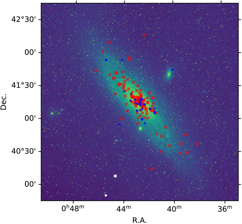
Figure 1: False-colour Digitized Sky Survey (DSS; Lasker et al., 1990) red mosaic of M 31 over-plotted with the positions of 135 spectroscopically confirmed M 31 Fe ii novae (red $\times$) and 38 He/N (including hybrids) novae (blue $+$); spectroscopic data from Shafter et al. (2011, and C. Ransome et al. in preparation). The white data points show the location of AT 2016dah (northern most; $\times$) and AT 2017fyp (southern most; $+$).

In this Paper we present follow-up observations of these novae located in the outer suburbs of M 31 and discuss the significance of their location within the M 31 GSS. In Section 2 we describe the observations of the novae. In Section 3 we go onto describe the results of the photometric, spectroscopic, and X-ray data analysis. Then in Section 4 we explore the association of AT 2016dah and AT 2017fyp with the M 31 GSS. Finally we discuss our findings in Section 5, before summarising our conclusions in Section 6. Throughout this Paper, all quoted uncertainties are to $1\sigma$ and all lower or upper limits are evaluated at $3\sigma$, unless otherwise stated.

2 Observations

2.1 AT 2016dah

Photometric observations of AT 2016dah were obtained using the 2.0 m fully robotic Liverpool Telescope (LT; Steele et al., 2004), La Palma, and the $48^{\prime\prime}$ Samuel Oschin telescope (P48) at Palomar. LT imaging was taken using the IO:O CCD camera (Smith & Steele, 2017) through $u^{\prime}BVr^{\prime}i^{\prime}$ filters, while P48 images were obtained using the CFH12K CCD mosaic camera through an $r^{\prime}$ filter. Additional photometric data were also obtained via the All-Sky Automated Survey for Supernovae (ASAS-SN; Shappee et al., 2014; Kochanek et al., 2017) Sky Patrol.

The LT photometric data were reduced using tools within the IRAF environment (Tody, 1993), and aperture photometry was performed using the qphot task. The LT data were calibrated against 81 stars in the field using photometry from Pan-STARRS (DR1; Chambers et al., 2016), these sources each had Pan-STARRS $griz$ magnitudes in the range $14\!<\!m\!<\!19$ (with catalogue uncertainties $\Delta m\!\leq\!0.1$). The $u^{\prime}$-band data were calibrated using a subset of 34 of those field stars that contained photometry in the range $14\!<\!u^{\prime}\!<\!19$ ($\Delta u^{\prime}\!\leq\!0.1$) from data release #12 of the Sloan Digital Sky Survey (SDSS; Alam et al., 2015). The photometry of the standards was converted from Sloan to Johnson magnitudes, where required, using the appropriate transformations from Jester et al. (2005). The subsequent LT photometry is reproduced in Table 8 and information about the secondary standards is presented in Table 5. A full overview of the photometric process employed is given in Darnley et al. (2007, 2016). The P48 (iPTF) data were obtained directly from that survey’s near real-time discovery pipeline (Cao, Nugent & Kasliwal 2016; Masci et al. 2017).

Spectroscopic observations were obtained using the SPRAT (Piascik et al., 2014) instrument on the LT operating in the blue-optimised mode. A slit width of $1^{\prime\prime}\!\!.8$ was used, resulting in a spectral resolution of $\sim$20 Å, or a velocity resolution of $\sim$1000 km s^-1. A log of the spectroscopic observations is provided in Table 1.

Table 1: Summary of all spectroscopic observations of AT 2016dah and AT 2017fyp with the SPRAT spectrograph on the Liverpool Telescope.

Date [UT]	$\Delta t$ [days]	Exposure [s]
AT 2016dah
2016 Jul 14.084	2.124	$2\times 600$
2016 Jul 14.135	2.175	$3\times 600$
2016 Jul 15.077	3.117	$3\times 600$
2016 Jul 16.107	4.174	$3\times 600$
2016 Jul 19.101	7.141	$3\times 600$
2016 Jul 26.135	14.115	$3\times 600$
2016 Aug 03.093	22.133	$3\times 600$
2016 Aug 05.109	24.149	$3\times 600$
2016 Aug 09.094	28.134	$2\times 600$
2016 Aug 13.113	32.153	$3\times 600$
2016 Aug 22.093	41.133	$3\times 600$
2016 Aug 29.050	48.090	$5\times 600$
2016 Sep 13.127	63.167	$2\times 600$
AT 2017fyp
2017 Aug 11.097	5.017	$3\times 600$
2017 Aug 13.018	6.938	$3\times 600$
2017 Aug 15.081	9.001	$3\times 600$
2017 Aug 17.132	11.052	$3\times 600$
2017 Aug 20.117	14.037	$3\times 600$
2017 Aug 26.105	20.025	$3\times 600$
2017 Sep 01.040†	25.960	$3\times 600$
2017 Sep 16.045	40.965	$3\times 900$
2017 Sep 30.126	55.046	$3\times 900$
2017 Oct 18.939	73.859	$3\times 900$
2017 Nov 12.912	98.832	$3\times 900$

• ^† The night of 2017 Aug 31 was non-photometric and this spectrum was collected through cloud. We have not included it in the analysis due to the poor signal-to-noise.

Initial reduction of the LT spectra, which includes bias subtraction, flat field correction, and sky subtraction, up to point of wavelength calibration, was performed using the SPRAT data reduction pipeline (see Barnsley, Smith & Steele 2012; Piascik et al. 2014). To perform relative flux calibration, we utilised 77 observations of the spectrophotometric standard star Hilt 102 (Stone, 1977), taken on photometric nights between 2017 June 19 and 2017 Dec 31, to construct a master sensitivity function. As the sensitivity function was constructed from data collected almost a year post-eruption, the absolute flux calibration was modified by comparison between bandpass spectrophotometry and the LT or iPTF $r^{\prime}$-band data. As such we estimate that the flux uncertainty of the AT 2016dah data is between 10–15%.

A Neil Gehrels Swift Observatory (Gehrels et al., 2004) target of opportunity (ToO) request was approved shortly after spectroscopic confirmation of AT 2016dah (Target ID: 34619). Beginning 6.6 d post-discovery, eleven approximately weekly Swift visits were utilised each with a target exposure time of 2 ks. The Swift UV/optical telescope (UVOT; Roming et al., 2005) was employed using the uvw1 filter ($\sim 2600$ Å). The Swift X-ray Telescope (XRT; Burrows et al., 2005) was also deployed, in the photon counting (PC) mode.

The Swift data were processed using the HEASoft (v6.26.1 for UVOT; v6.22 for XRT) software and the corresponding calibration files. UVOT magnitudes were calculated using the uvotsource tool, with a standard 5^′′ radius circular extraction region for the source, and a 46^′′ radius circular aperture offset from, but close to ($\alpha=0^{\mathrm{h}}44^{\mathrm{m}}43^{\mathrm{s}}$, $\delta=40^{\circ}09^{\prime}34^{\prime\prime}$), the source used to estimate the background. The UV emission had faded below detectability by the end of September. The XRT data were analysed using the freely available on-line tool (Evans et al., 2009). No X-ray source corresponding to AT 2016dah was detected at any time (also see Chinetti et al., 2016b). Results from the UVOT and XRT analysis are presented in Table 2.

Table 2: Neil Gehrels Swift Observatory XRT and UVOT observations of AT 2016dah and AT 2017fyp.

Date	$\Delta t$	MJD $57000+$		Exposure	XRT (0.3–10 keV)		UVOT uvw1	Obs. ID
[UT]	[days]	Start	End	timea [s]	[counts sec-1]	$L$ [$10^{36}$ erg s-1]	[mag]b
AT 2016dah
2016 Jul 19.377	7.417	588.008	588.746	2041.8	$<0.008$	$<\phantom{0}3.6$	$17.12\pm 0.03$	00034619002
2016 Jul 26.278	14.318	595.237	595.319	2044.1	$<0.005$	$<\phantom{0}2.3$	$18.00\pm 0.05$	00034619003
2016 Aug 03.621	22.661	603.356	603.887	1183.4	$<0.032$	$<14.4$	$18.25\pm 0.07$	00034619004
2016 Aug 11.903	30.943	611.864	611.941	1847.0	$<0.006$	$<\phantom{0}2.7$	$19.11\pm 0.09$	00034619005
2016 Aug 20.677	39.717	620.642	620.712	1181.8	$<0.007$	$<\phantom{0}3.2$	$19.36\pm 0.13$	00034619006
2016 Sep 04.695	54.735	635.654	635.736	2066.8	$<0.004$	$<\phantom{0}1.8$	$20.26\pm 0.19$	00034619007
2016 Sep 12.799	62.839	643.768	643.830	1281.0	$<0.019$	$<\phantom{0}8.5$	$20.49\pm 0.29$	00034619008
2016 Sep 20.773	70.813	651.732	651.814	1902.2	$<0.007$	$<\phantom{0}3.2$	$20.50\pm 0.23$	00034619009
2016 Sep 29.772	79.812	660.767	660.778	954.5	$<0.044$	$<19.8$	…c	00034619011
2016 Oct 02.889	82.929	663.888	663.889	116.3	$<0.157$	$<70.6$	$>19.2$	00034619012
2016 Oct 06.714	86.754	667.675	667.752	1966.5	$<0.005$	$<\phantom{0}2.3$	($21.09\pm 0.38$)d	00034619013
AT 2017fyp
2017 Aug 24.802	18.722	989.702	989.901	1836.0	$<0.015$	$<\phantom{0}6.2$	$16.40\pm 0.03$	00010239001
2017 Sep 07.101	32.021	1003.002	1003.200	451.2	$<0.021$	$<\phantom{0}8.7$	$17.14\pm 0.06$	00010239002
2017 Sep 14.504	39.424	1010.368	1010.641	1401.0	$<0.020$	$<\phantom{0}8.2$	$17.73\pm 0.05$	00010239003
2017 Oct 18.279	73.199	1044.116	1044.441	3695.4	$<0.003$	$<\phantom{0}1.2$	$18.65\pm 0.05$	00010239004
2017 Nov 18.190	104.110	1075.115	1075.264	4049.2	$<0.002$	$<\phantom{0}0.8$	$19.36\pm 0.08$	00010239005
2017 Dec 18.593	134.513	1105.224	1105.962	3149.9	$<0.004$	$<\phantom{0}1.6$	$20.43\pm 0.17$	00010239006
2018 Jan 18.776	165.696	1136.773	1136.778	425.9	$<0.051$	$<21.0$	$>20.0$	00010239007
2018 Jan 20.492	167.412	1138.490	1138.494	322.7	$<0.025$	$<10.3$	$>19.6$	00010239008
2018 Jan 21.961	168.881	1139.760	1140.162	1153.8	$<0.011$	$<\phantom{0}4.5$	$>20.5$	00010239009
2018 Jan 23.920	170.840	1141.887	1141.953	2209.9	$<0.006$	$<\phantom{0}2.5$	$>20.9$	00010239010
2018 Jan 18–24e	168.284	1136.773	1141.953	3822.3	$<0.003$	$<\phantom{0}1.2$	$>21.2$	…007—010

• ^aHere the exposure time refers specifically to UVOT.

• ^bUVOT magnitudes are reported in the Vega system, we quote the random statistical uncertainties, calibration systematic uncertainties are 0.03 mag.

• ^cNo useable data due to loss of star tracker lock.

• ^dSource detection significance at the nova position was at $2.9\sigma$.

• ^eHere we combine the final four Swift observations as they were taken within a one week period.

For each Swift XRT observation, we have also estimated the upper luminosity limit of the source (0.3–10 keV). Here we assumed a distance to M 31 of $d=752\pm 17$ kpc (Freedman et al., 2001), an estimate of the Galactic neutral atomic H density $n_{\mathrm{H}}=5.32\times 10^{20}\,\mathrm{cm}^{-2}$ (HI4PI Collaboration et al., 2016), and a typical (for X-ray detected M 31 novae) blackbody temperature of $kT=50$ eV (Henze et al., 2014). Luminosity limits were estimated using the web interface to PIMMS (v4.10b) and are recorded in Table 2.

2.2 AT 2017fyp

The LT photometric data for AT 2017fyp were reduced in a similar manner as those for AT 2016dah. Here, the LT data were calibrated against 42 stars in the field using photometry from SDSS DR12, these sources each had Sloan $u^{\prime}g^{\prime}r^{\prime}i^{\prime}z^{\prime}$ magnitudes in the range $14\!<\!m\!<\!19$ ($\Delta m\!\leq\!0.1$). The subsequent LT photometry is reproduced in Table 11 and information about the secondary standards is presented in Table 7.

The Las Cumbres Observatory (LCO; Brown et al., 2013) 2.0 m telescope at Haleakala (formally the Faulkes Telescope North) was used to collect four additional epochs of $BVr^{\prime}i^{\prime}$ photometry. These data were taken using the Spectral camera and were reduced and analysed in an identical manner to the LT imaging data. The LCO photometry is also recorded within Table 11.

Additional photometric data for AT 2017fyp, limited to the pre-discovery and discovery photometry, were obtained from the ATLAS survey (Tonry et al., 2017). Three Gaia photometry points are also available.

The LT SPRAT spectroscopic data were reduced in an identical manner to those for AT 2016dah, and we employed the same sensitivity function to produce relative flux calibrated spectra. However, for these data, no discernible improvement in the absolute flux calibration was found by using bandpass spectrophotometry, in part this was due to the lower photometric cadence. We estimate the flux uncertainty of the AT 2017fyp data is between 15–20%.

A Swift ToO programme was also rapidly approved post-discovery for AT 2017fyp (Target ID: 10239) and a series of ten observations commenced two weeks post-discovery. These Swift XRT and UVOT data were reduced in an identical fashion to those for AT 2016dah. For the UVOT photometry, a circular background estimation region of radius 67^′′ was positioned at $\alpha=0^{\mathrm{h}}45^{\mathrm{m}}34^{\mathrm{s}}$, $\delta=39^{\circ}49^{\prime}25^{\prime\prime}$. Like AT 2016dah, no X-ray source was detected, here upper luminosity limits were derived assuming an average Galactic column of $n_{\mathrm{H}}=4.73\times 10^{20}\,\mathrm{cm}^{-2}$. The AT 2017fyp swift results are also reported in Table 2. The final four Swift visits were obtained within a single week, combining them does not yield either an XRT or UVOT detection at that time.

2.3 Archival data

To enable a search for the progenitor systems of AT 2016dah and AT 2017fyp, i.e. the quiescent novae, we utilised a number of archival observations. The positions of both AT 2016dah and AT 2017fyp are located within Field 7 of the Canada-France-Hawaii Telescope (CFHT) survey of the M 31 GSS McConnachie et al. (2003, also see Sections 4 and 5.6). These data were taken using the CFH12K instrument, a $12,288\times 8,192$ pixel CCD mosaic camera (Cuillandre et al., 2000) and consist of a pair of $3\times 545$ s exposures through Mould $V$ and $I$-band filters. The CFHT data were collected on 2001 September 13, $\sim 15$ yrs before the eruptions. AT 2016dah lies within chip02 of Field 7, whereas AT 2017fyp can be found within chip09. As the field of view of each of the CFH12K chips is roughly similar to the LT field, these data were processed in a similar fashion to the LT data, including stacking of each set of three images, and photometry was performed as described above. We also utilised the Galaxy Evolution Explorer (GALEX; Martin et al., 2005) data archive to extend the search to the near- and far-UV.

A search for potential progenitor/quiescent systems was performed following the procedure set out in Bode et al. (2009), and then further refined by Williams et al. (2014) and more recently Healy et al. (2019). Astrometric solutions were computed between each $V$ and $i^{\prime}$-band LT observation and the corresponding CFHT $V$ and $I$-band stack, and the GALEX data, to define the progenitor search region with those data.

3 Results

3.1 Time of eruption

Although the last pre-discovery observation of AT 2016dah was taken in the $V$-band by ASAS-SN on 2016 Jul 11.52 UT, this observation was not of sufficient depth to rule out an eruption. Therefore, we assume that the eruption occurred between the last iPTF non-detection ($R>21.171$) on Jul 11.48 and the iPTF detection ($R=18.78\pm 0.07$) on Jul 12.44. For the purpose of our analysis, we take the time of eruption to be 2016 Jul $11.96\pm 0.48$ UT (MJD: $57580.96\pm 0.48$).

AT 2017fyp was observed by ATLAS on 2017 Aug 04.603 UT; no source was detected down to a limit of 19.28 mag (through the ATLAS orange filter). We again assume that the eruption occurred at some point between that observation and the discovery observation, also by ATLAS, on Aug 07.553. Therefore we take the time of eruption of AT 2017fyp to be 2017 Aug $6.08\pm 1.48$ UT (MJD: $57971.08\pm 1.48$).

3.2 Reddening

The general Galactic reddening toward M 31 was determined as $E\left(B-V\right)=0.1$ (Stark et al., 1992). Schlegel, Finkbeiner & Davis (1998) find $E\left(B-V\right)=0.06$ and 0.05 around the positions of AT 2016dah and AT 2017fyp, respectively. Converting the Galactic $n_{\mathrm{H}}$ estimates (see Section 2) to reddening (using Equation 1 from Güver & Özel, 2009, and assuming $R_{V}$=3.1) we find $E\left(B-V\right)=0.08$ and 0.07 for AT 2016dah and AT 2017fyp, respectively. There are no reliable reddening markers available for nova photometry, and there are none present in our obtained spectra with which we could independently constrain the reddening toward either system. Some authors have used the Balmer decrement to estimate the reddening for particular novae, however others (see, for e.g., for a recent discussion Williams, Darnley & Henze, 2017) have shown this to be unreliable. As such, we will assume a reddening of $E\left(B-V\right)=0.1$ toward both novae. Given that both novae are located far from the M31 disk, we assume that there is negligible extinction contribution beyond the confines of the Milky Way. All spectra have been dereddened using this value, and all subsequent discussion of the spectra refer to analysis of the dereddened observations.

3.3 Photometric evolution

3.3.1 AT 2016dah

The combined ASAS-SN, iPTF, LT, and Swift UVOT light curve of the eruption of AT 2016dah are shown in Figure 2. These light curves reveal a nova that was detected on the rise (still relatively uncommon for extragalactic novae, particularly those beyond the Magellanic Clouds), that in general follows a rapid and smooth decline through around six magnitudes (before it became undetectable). The Strope, Schaefer & Henden (2010) light curve scheme would classify AT 2016dah as a smooth or “S”-type nova.

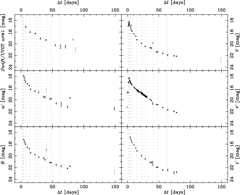
Figure 2: The near-UV—optical light curve of nova AT 2016dah. The epochs of spectroscopy are also indicated by the vertical grey-dotted lines. Grey data points indicate detections with significance $2<\sigma\leq 3$.

In Figure 3 we present the $r^{\prime}$-band light-curve (red) of AT 2016dah, plotted on a logarithmic time axis. The three straight-line fits to these data, demonstrate that the $r^{\prime}$-band evolution follows three broken power-laws (between flux and time; $F\propto t^{\alpha}$). The post-maximum break occurs at around $22.5$ d post-eruption, before the break the slope is $\alpha=-1.00\pm 0.01$; post-break, $\alpha=-2.55\pm 0.06$. We note that neither value is consistent with those determined by (Hachisu & Kato, 2006). The slope of the $r^{\prime}$-band light cure before maximum light is $\alpha=1.41\pm 0.01$.

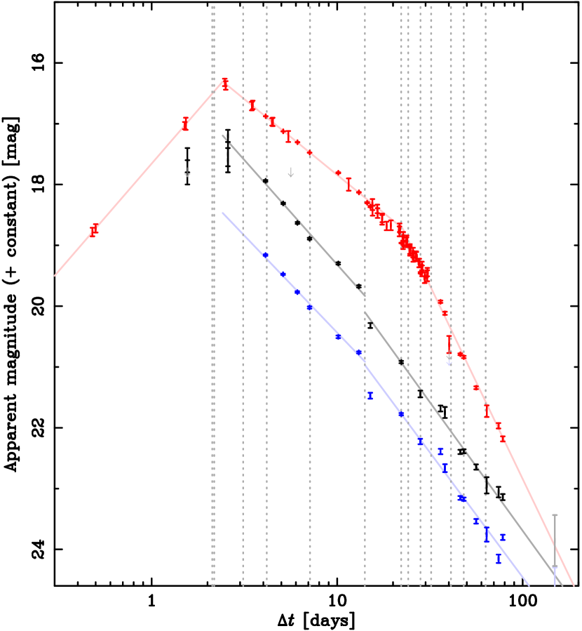
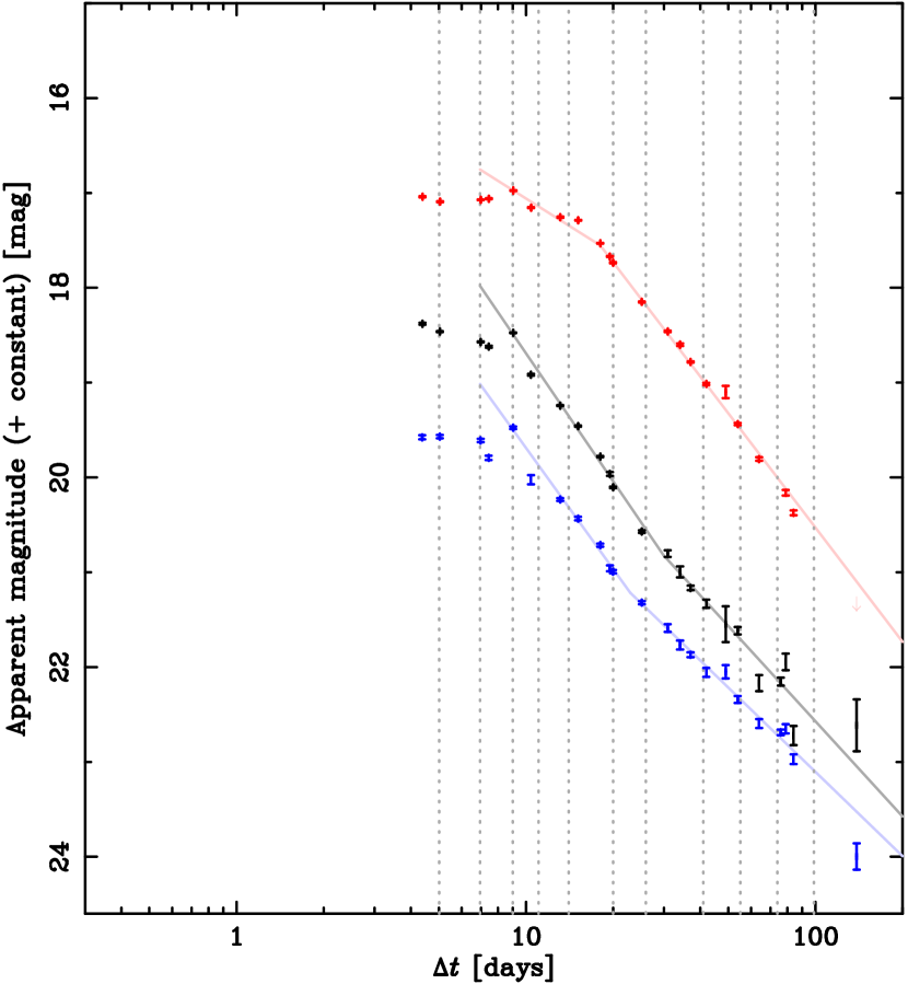
Figure 3: Light curve of AT 2016dah (left) and AT 2017fyp (right) displayed with logarithmic time axes. The $r^{\prime}$-band light curve is shown in red (top), $V$-band in black (middle; all magnitudes shifted by $+1$), an $B$-band in blue (bottom; shifted by $+2$). The broken power-law fits to these data ($F\propto t^{\alpha}$) are discussed in the text. The vertical dotted lines indicate spectroscopic epochs.

Figure 3 also shows the $V$-band (black) and $B$-band (blue) light-curves. While much less densely sampled than the $r^{\prime}$-band data, these light curves follow a similar form, with one marked difference. There is an apparent ‘discontinuity’ in the light curves at around day 14 (a spectrum was also taken at this time, see Section 3.4.1), where there is a ‘sudden’ drop in the brightness by just over half a magnitude. This drop appears also appears in the $u^{\prime}$-band and there is a non-conclusive hint of such an occurrence in the Swift UVOT data, but is not present in the two reddest filters. The $V$ and $B$-band data from maximum light until this drop are consistent with power-law of indices of $\alpha_{V}=-1.38\pm 0.06$ and $\alpha_{B}=-1.30\pm 0.05$, respectively, i.e. they are consistent with each other, but not with the $r^{\prime}$-band decline during this phase. Post-drop, the $V$ and $B$-band declines remain consistent with indices of $\alpha_{V}=-1.69\pm 0.05$ and $\alpha_{B}=-1.65\pm 0.07$, respectively. Both these later time $V$ and $B$-band declines are consistent with the power-law slopes expected during this period between $\sim 2$ to $\sim 6$ magnitudes below peak ($\alpha=-1.75$; Hachisu & Kato, 2006).

For the purpose of this analysis, we will assume that maximum light occurred at the time of the brightest $r^{\prime}$-band observation, $r^{\prime}=16.32\pm 0.06$, 2.48 d post-eruption. A pair of spectra taken $0.33$ d earlier (see Section 3.4.1) are consistent with pre-maximum evolution, a spectrum taken at $\Delta t=3.117$ shows the nova in a post-maximum state. As such, we can use the power-law fits to derive the following estimates of the $t_{2}$ and $t_{3}$ decline times (the time taken to decay by two and three magnitudes, respectively, from peak): $t_{2}\left(r^{\prime}\right)=13.3^{+0.6}_{-0.3}$ d (a decay rate of $\sim 0.15$ mag d^-1); $t_{3}\left(r^{\prime}\right)=26\pm 2$ d and occurs $\sim 6$ d post-break. Such decline times would class AT 2016dah as a fast nova (Payne-Gaposchkin, 1964). For the $V$ and $B$-bands we find, $t_{2}\left(V\right)=7\pm 1$ d, $t_{2}\left(B\right)=8\pm 1$ d, $t_{3}\left(V\right)=13\pm 1$ d, $t_{3}\left(B\right)=16^{+3}_{-2}$ d. These values are smaller than those computed using the $r^{\prime}$-band data, whose decline is slowed by the persistence of the H$\alpha$ emission line. The $V$ and $B$-band values classify AT 2016dah as a very fast nova, the $V$-band value for $t_{3}$ is consistent with the epoch of the light curve ‘drop’, the uncertainty on the $B$-band $t_{3}$ is larger due to the lack of observations at maximum light, but it is formally also consistent with the drop.

The light curve of AT 2016dah was followed for around 150 days post-eruption, at which point the nova was detected $\sim 6$ magnitudes below peak in the $u^{\prime}$-band, and was marginally detected (sub $3\sigma$) with a similar amplitude in the $V$ and $B$-bands.

3.3.2 AT 2017fyp

In Figure 4 we present the ATLAS, LCO, LT, and Swift/UVOT photometric light curves of AT 2017fyp. At first inspection, the evolution of AT 2017fyp is clearly slower than that of AT 2016dah, and it is around $\sim 1$ mag fainter at peak. There is no coverage of the rise, and maximum light may have been missed, but the light curve appears to have a short flat-top peak lasting around $\sim 5$ d. Following this flat period, the nova enters a rapid decline until a clear break in the light-curve at $\sim 25$ d post-eruption where the decline slows. AT 2017fyp was followed for $\sim 140$ d post-eruption through a decay of 4–5 magnitudes, after which it remained detected in the bluer bands (and was marginally detected, $<3\sigma$, in the $i^{\prime}$-band). Given the flat topped nature, and power-law like decline (see below), AT 2017fyp may be best classed as a flat topped or “F”-type nova. A slight increase in the luminosity of the nova during this maximum light ‘plateau’ phase is evident, particularly to the blue.

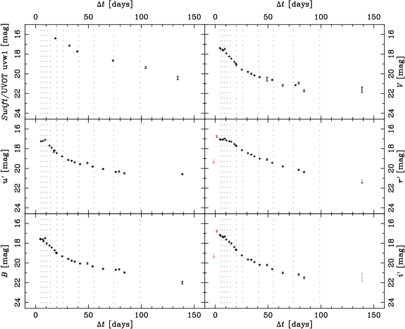
Figure 4: The near-UV—optical light curve of nova AT 2017fyp. The epochs of spectroscopy are also indicated by the vertical grey-dotted lines. Grey data points indicate detections with significance $2<\sigma\leq 3$. The red data points included in the $r^{\prime}$ and $i^{\prime}$ indicate the ATLAS orange filter pre-discovery upper-limit and discovery photometry; the orange filter has a wide bandpass that covers $r^{\prime}+i^{\prime}$. The final four Swift data points ($\Delta t>50$ d; see Table 2) are not shown, all four are upper limits consistent with the expected late-decline of the eruption.

As with AT 2016dah, we present the $BVr^{\prime}$-band light curves of AT 2017fyp in Figure 3, where they are plotted against a logarithmic time axis. Here the flat topped nature is evident, as is the broken-power law decline, with that break in the opposite direction in the $V$ and $B$-bands to that of AT 2016dah (steep to shallow, for AT 2017fyp, versus shallow to steep for AT 2016dah). Here the $r^{\prime}$-band behaviour is again probably driven by the H$\alpha$ emission line evolution.

The initial indices of the $BVr^{\prime}$-band power-law declines are $\alpha=-1.69\pm 0.07$, $-1.79\pm 0.06$, and $-0.77\pm 0.08$, respectively. Here the $V$ and $B$-band slopes are consistent with those determined by Hachisu & Kato (2006), but over an earlier part of the light curve development (as measured by decline from peak) as suggested by those authors. The later portion of the decline is consistent with power-law indices of $\alpha=-1.18\pm 0.04$, $-1.35\pm 0.05$, and $-1.60\pm 0.04$, for the $BVr^{\prime}$-bands, respectively.

With novae with flat topped or cusp-like (“C”-type) behaviour around peak, it is always a bone of contention how one should determine the epoch of maximum light, and hence how to reliably estimate the decline times. For this analysis, we will assume that maximum light occurred at some point during the $\sim 5$ d flat top (but no later than $\Delta t\approx 9$ d post-eruption), and that the decline time range is determined by the power-law decline and the width of the flat top. As such, we estimate the following decline times: $32\lesssim t_{2}\left(r^{\prime}\right)\lesssim 37$ d, $16\lesssim t_{2}\left(V\right)\lesssim 21$ d, $20\lesssim t_{2}\left(B\right)\lesssim 25$ d, $63\lesssim t_{3}\left(r^{\prime}\right)\lesssim 68$ d, $38\lesssim t_{3}\left(V\right)\lesssim 43$ d, and $53\lesssim t_{3}\left(B\right)\lesssim 58$ d. The $V$ and $B$-band decline times would class AT 2017fyp as a fast nova, whereas the slower $r^{\prime}$-band times would class this eruption as moderately fast, again the influence of the H$\alpha$ emission line will have impacted the $r^{\prime}$-band estimates.

3.4 Spectroscopic evolution

3.4.1 AT 2016dah

A series of thirteen spectra of AT 2016dah were obtained by the SPRAT instrument on the LT. The first being captured at 2016 Jul 14.084 UT, just 2.12 d post-eruption. That spectrum, and a second obtained 0.05 d later (see the black and red spectra – the two most luminous – in the top panel of Figure 5), are both consistent with the early optically thick ‘fireball’ phase of a nova eruption (Chinetti et al., 2016a). These spectra were observed $\sim 0.33$ d before $r^{\prime}$-band maximum light (see Figure 2). This pair of spectra exhibit weak Balmer emission with the H$\alpha$–H$\delta$ line profiles all containing P Cygni absorption troughs to the blue. The H$\alpha$ absorption minimum is consistent with a velocity of $-1200\pm 200$ km s^-1, with respect to the mean emission peak (see below). Whereas the terminal velocity of the H$\alpha$ P Cygni is at $2300\pm 400$ km s^-1 blueward of the mean peak. These spectra display a blue continuum with relatively few other features. The continuum may be punctuated by blue-shifted absorptions from Fe ii multiplets 42 and 74. At this stage emission from O i (1) 7774 Å is already present. A fit to the continua of this pair of spectra shows that they are consistent with the form of a black body with effective temperature $\approx 10,000$ K.

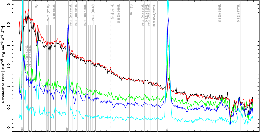
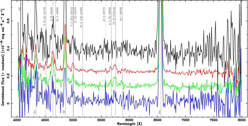
Figure 5: The Liverpool Telescope SPRAT optical spectra of nova AT 2016dah. Top: Optically thick fireball and early decline ‘principle’ Fe ii spectra. Spectra from brightest to faintest: 2.150 d post-eruption (black); 3.117 d (red); 4.174 d (green); and 7.141 d (blue). Bottom: Transition from principle spectra to Orion phase. Brightest to faintest: 14.115 d post-eruption (black); 22.133 d (red); 24.149 d (green); and 28.134 d (blue). These four spectra have been offset in flux for clarity by integer multipliers of $0.1\times 10^{-15}$ erg cm^-2 s^-1 Å^-1.

A Gaussian profile combined with a linear function was used to simultaneously fit the line flux and local continuum for the Balmer emission lines (H$\alpha$–H$\gamma$; the low signal-to-noise and line blanketing, due to the low spectral resolution to the blue, rendered fits to H$\delta$ uninformative). The resultant line fluxes are reproduced in Table 3. The evolution of the Balmer emission line fluxes and that of the H$\alpha$ line profile are shown in the top-panel of Figure 6. The Balmer emission peaks much later than the broad-band maximum light (which occurs at $\Delta t=2.48$ days post-eruption). Following a slow increase in flux, the Balmer emission peaks around day 7 post-eruption. After peak, the Balmer emission follows a roughly linear decline (see Figure 6). We measure the weighted average emission line centre of H$\alpha$ from all thirteen spectra to be at $-420\pm 30$ km s^-1 (after heliocentric correction) with respect to the rest-wavelength of H$\alpha$, which corresponds to a redshift of $z=\left(-1.4\pm 0.1\right)\times 10^{-3}$. The weighted average FWHM of H$\alpha$ across the thirteen spectra is $2300\pm 70$ km s^-1. Other than during the first two epochs, where the H$\alpha$ profile has a P Cygni form, there is not significant evolution of the FWHM through the spectral sequence. In general, the H$\alpha$ profile is Gaussian-like, which is fairly typical for Fe ii novae.

Table 3: Selected emission line fluxes from the Liverpool Telescope SPRAT spectra of AT 2016dah and AT 2017fyp.

	Dereddened flux
$\Delta t$ [days]	[$\times 10^{-15}$ erg cm-2 s-1]
	H$\alpha$	H$\beta$	H$\gamma$
AT 2016dah
2.124a	$\phantom{0}\phantom{0}8\pm 3$	$\phantom{0}16\pm 3$	$\phantom{0}7\pm 2$
2.175a	$\phantom{0}\phantom{0}8\pm 3$	$\phantom{0}17\pm 5$	($5\pm 3$)
3.117	$\phantom{0}52\pm 3$	$\phantom{0}54\pm 5$	$40\pm 7$
4.174	$111\pm 3$	$\phantom{0}93\pm 6$	$64\pm 6$
7.141	$183\pm 3$	$\phantom{0}85\pm 4$	$43\pm 6$
14.115	$136\pm 3$	$\phantom{0}35\pm 3$	$18\pm 4$
22.133	$\phantom{0}66\pm 1$	$\phantom{0}16\pm 1$	$\phantom{0}8\pm 1$
24.149	$\phantom{0}69\pm 2$	$\phantom{0}16\pm 1$	$12\pm 2$
28.134	$\phantom{0}50\pm 2$	$\phantom{0}11\pm 2$	($7\pm 4$)
32.153	$\phantom{0}39\pm 1$	$\phantom{0}10\pm 2$	$\phantom{0}7\pm 2$
41.133	$\phantom{0}15\pm 1$	$\phantom{0}\phantom{0}3\pm 1$	($3\pm 2$)
48.090	$\phantom{0}13\pm 1$	$\phantom{0}\phantom{0}3\pm 1$	($3\pm 1$)
63.167	$\phantom{0}\phantom{0}2\pm 1^{\mathrm{b}}$	00…	…
AT 2017fyp
5.017	$202\pm 7$	$130\pm 10$	$60\pm 10$
6.938	$310\pm 10$	$140\pm 20$	$75\pm 7$
9.001	$420\pm 20$	$160\pm 20$	$90\pm 20$
11.052	$440\pm 20$	$140\pm 20$	$78\pm 9$
14.037	$350\pm 20$	$100\pm 9$	$49\pm 6$
20.025	$300\pm 10$	$\phantom{0}60\pm 4$	$31\pm 4$
40.965	$\phantom{0}92\pm 5$	$\phantom{0}22\pm 2$	$17\pm 3$
55.046	$\phantom{0}53\pm 3$	$\phantom{0}12\pm 2$	$14\pm 3$
73.859	$\phantom{0}39\pm 2$	$\phantom{0}\phantom{0}8\pm 2$	$14\pm 3$
98.832	$\phantom{0}21\pm 1$	$\phantom{0}\phantom{0}5\pm 2$	$\phantom{0}6\pm 1$

• All emission line fluxes and uncertainties were determined through fitting a Gaussian profile to the line in velocity space. Values in parenthesis are lines for which the flux uncertainties lie between 2 and $3\sigma$.

• ^aIn these spectra the Balmer lines have P Cygni profiles, here we report the flux of the emission component.

• ^bFormally, the flux was constrained marginally beyond $3\sigma$.

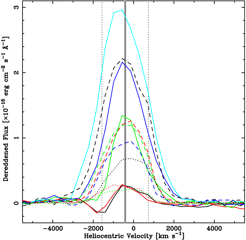
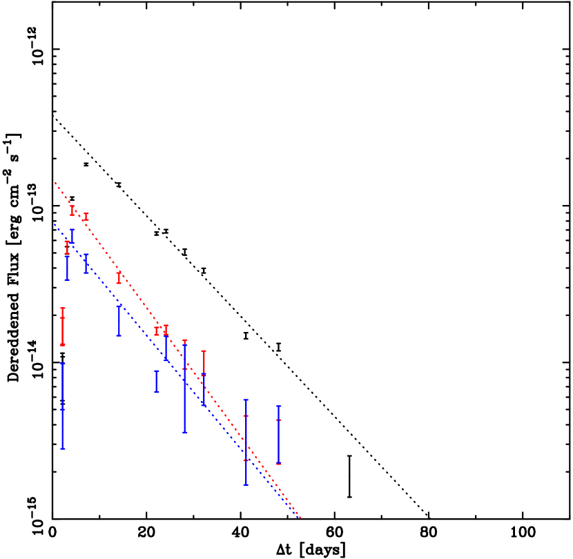
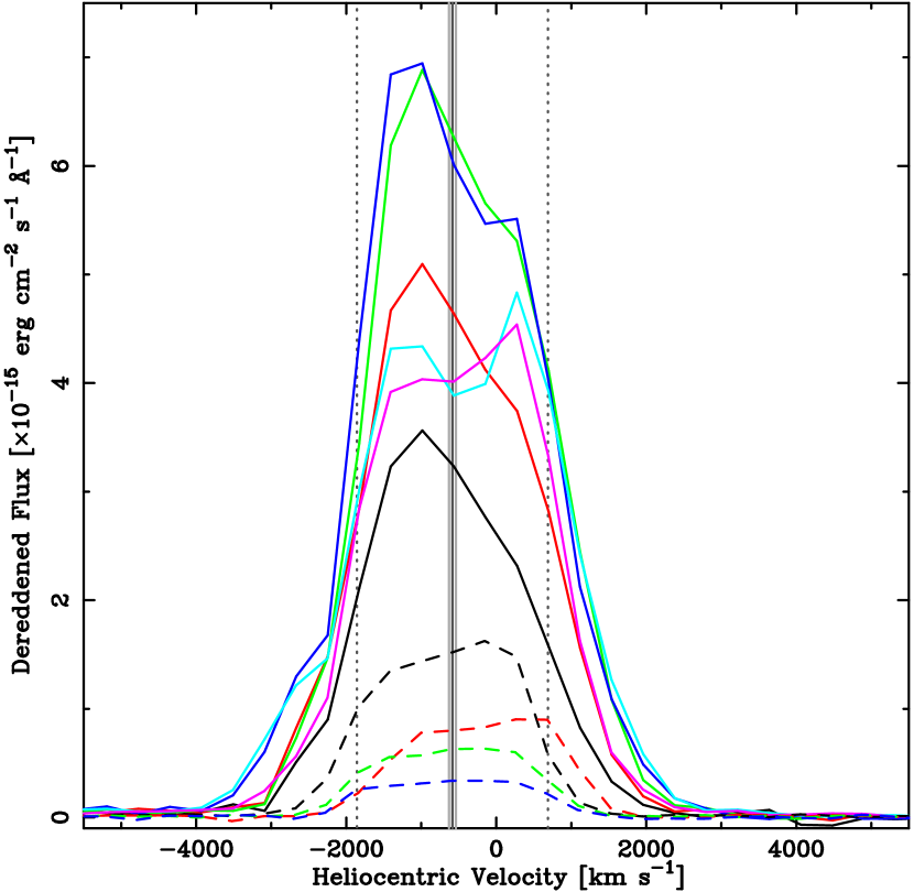
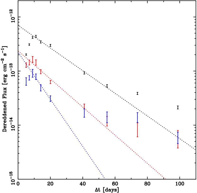
Figure 6: Left: H$\alpha$ line profile evolution for AT 2016dah (top) and AT 2017fyp (bottom) following continuum subtraction and Heliocentric correction. The line colours are consistent with those used in Figures 5, 7 and 8. The solid and dashed lines relate to the spectra in the top and bottom panels of Figures 5, 8, respectively, the dotted lines (AT 2016dah only) relate to those spectra shown in 7. The vertical solid lines indicate the measured average line centre (and uncertainties), the vertical dotted lines indicate the extent of the measured average FWHM. Right: The flux evolution of the H$\alpha$ (black), H$\beta$ (red), and H$\gamma$ emission lines for AT 2016dah (top) and AT 2017fyp (bottom). The dotted lines indicate linear fits to portions of those data (see text).

The following three spectra were taken, 3.12 d, 4.17 d, and 7.14 d post-eruption (see green, blue, and cyan, respectively, spectra in the top panel of Figure 5) and were all collected between maximum light and $t_{2}$, with the last of this sub-set taken just over 1 magnitude below peak. Here there is a clear transition from the fireball phase to the ‘principle’ spectrum. The continuum emission weakens across the sub-set, it is no longer black-body like, and is shallower than that expected from a Rayleigh-Jeans tail. Throughout this stage the continuum slope is not consistent with that expected from free-free emission (see Wright & Barlow, 1975). The Balmer series has transitioned from their initial P Cygni profiles to strong emission lines that contribute substantially to the total optical emission. The Fe ii (42) triplet is the next strongest feature, with emission also detected from Fe ii (26, 27, 37, 38, 48, 49, 74). Given the lack of Fe ii (74) 6248 Å, the Fe ii (74) 6148 Å line is probably blended with O i 6157 Å. Emission from O i (1) 7774 Å remains present and is joined by weak Si ii 6347/6371 Å and Na i (D) lines. Emission from N i (3) at $\approx 7452$ Å also becomes visible at this time. These spectra are consistent with the nova being a member of the Fe ii taxonomic spectral class (Williams, 1992, 2012). The latter spectra of this sub-set show evidence for the appearance of emission from N iii 4640 Å (from day 4.17) and N ii (3) 5680 Å (from day 7.14). The apparent presence of [O i] 5577 Å is most likely the residual from sky-subtraction.

The next set of four spectra were collected between two-weeks and four-weeks post-eruption (see the bottom panel of Figure 5) and span the epoch of $t_{2}$ to approximately $t_{3}$. Here the systemic fading and flattening of the continuum has continued and the Balmer emission has weakened. The Fe ii (42) emission remains at day 14.12, but no Fe ii emission is evident from day 22 onward. Could the ‘drop’ seen in the $B$ and $V$-band light curves around day 14 (see Section 3.3.1) be solely due to the weakening of the Fe ii emission, as the Balmer decline is smooth during this phase (see Figure 6)? Emission lines of N ii 5001, 5680 Å and N iii 4517, 4640 Å are visible throughout this set (also see Chinetti et al., 2016b). The N ii 5001 Å is seen to visibly strengthen compared to the neighbouring H$\beta$ line. There is evidence for the appearance of [N ii] 5755 Å from day 14, along with He i 5876 Å. The diminishing signal-to-noise in these spectra obscures any O i line that may still be present. There is tentative evidence for the He ii 4686 Å line appearing from day 14. The movement of the flux ratio of H$\beta$:N ii 5001 Å toward the N line (around half the H$\beta$ flux by day 28) could also suggest that the [O iii] 5007 Å nebular line may be be present and strengthening.

The final sub-set of four spectra (see Figure 7) were taken between day 32 and 63 post-eruption, these range from just post-$t_{3}$ to around five magnitudes below peak. The continuum continues to fade, remaining just detected in the final spectrum, the Balmer flux continues to fade. Other prominent lines include the N iii 4640 Å feature (the Bowen-blend), and a line at around 5000 Å that rivals the flux of H$\beta$ and is most likely [O iii] 5007 Å. Other lines present include He i 5876, 6678, 7065 Å, He ii 4686 Å, N ii 5680 Å  [N ii] 5755 Å, N iii (3) 4517 Å, and possibly [Fe ii] 4244, 5159 Å, and [O iii] 4959 Å. As such, AT 2016dah becomes one of a small handful of extragalactic novae to have been detected in their nebular phase.

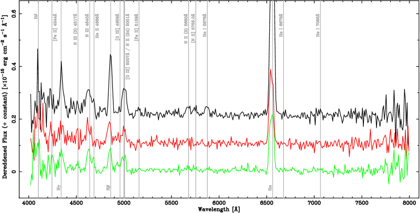
Figure 7: The Liverpool Telescope SPRAT optical spectra of nova AT 2016dah. These spectra show the nebular phase of the eruption. Brightest to faintest: 32.153 d post-eruption (black); 41.133 d (red); and 48.090 d (green). These three spectra have been offset in flux for clarity by integer multipliers of $0.1\times 10^{-15}$ erg cm^-2 s^-1 Å^-1. The spectrum from 2016 Sep 13 ($\Delta t=63.167$ d) is not shown due to its low signal-to-noise.

3.4.2 AT 2017fyp

The spectral coverage of AT 2017fyp began later than that of AT 2016dah. The first spectrum of this eruption was obtained 5 days post eruption and began a series of eleven spectra all collected by SPRAT on the LT. As discussed in Section 3.3.2, the light curve of AT 2017fyp either indicates a slow rise to peak, or alternatively an approximately flat topped profile. In either event the evolution during the first three spectra, taken on days 5, 7, and 9 (black, red, and green spectra in the top panel of Figure 8), is consistent with the slight increase in photometric flux (particularly in the blue) seen during this stage. These three and the remaining three in this sub-set, which were taken 11, 14, and 20 days post-eruption (the blue, cyan, and magenta spectra, respectively), were all collected between maximum light and approximately $t_{2}$. Following the initial rise in continuum luminosity there follows a systemic decline in flux. All these spectra are dominated by Balmer emission, and there is no evidence for absorption components in the earlier spectra. This would seem to suggest that the light curve is indeed flat topped, rather than this stage being a slow rise to maximum (with the continuum still optically thick). The width of the H$\alpha$ line in the first epoch is $2440\pm 60$ km s^-1. Emission lines from Fe ii (42) are particularly prominent; those from multiplets 26, 27, 37, 38, 48, 49, and 74 are also present. A line at $\sim 5530$ Å may be due to Fe ii (55) or could be Mg i (9) 5528 Å. The O i (1) 7774 Å line is present as is the Si ii doublet. However, throughout this whole sub-set the following lines are also clearly present: He i 5876, 7065 Å, N ii (3) 5680 Å, N iii 4640 Å, and possibly He ii 4686 Å (although, at this early stage, this line may actually be O ii 4650 Å; see, for e.g., Harvey et al., 2018). As such, these spectra best fit the hybrid taxonomic class (also see Hosseinzadeh et al., 2017); although a good number of hybrids display a transition between spectral types, rather than displaying both so prominently for an extended period. Over this period the slope of the continuum (albeit hard to define unambiguously) appears roughly consistent with that expected for optically thin free-free emission, as early as day 5 post-eruption.

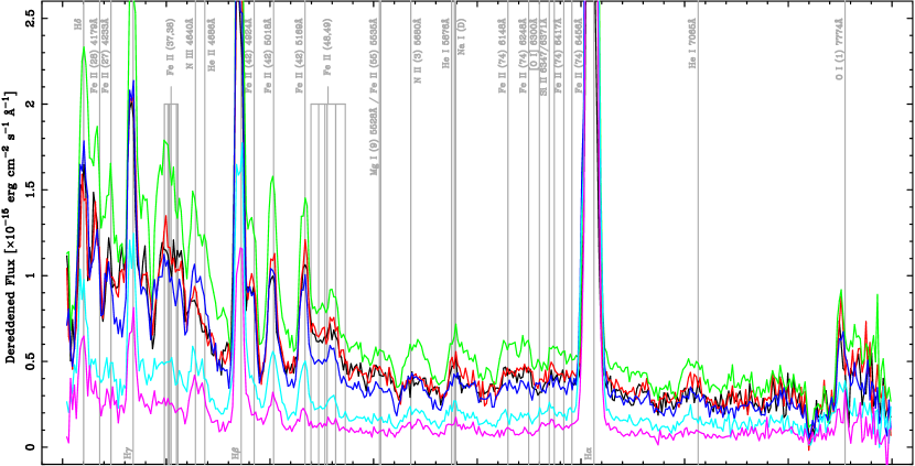
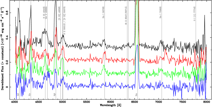
Figure 8: The Liverpool Telescope SPRAT optical spectra of nova AT 2017fyp. Top: The principle Fe ii+He/N (hybrid) spectra during the early decline spectra. Spectral sequence: 5.017 d post-eruption (black); 6.938 d (red); 9.001 d (green); 11.052 d (blue); 14.037 d (cyan); and 20.025 d (magenta). Bottom: Transition from Orion to nebular spectra. Brightest to faintest: 40.965 d post-eruption (black); 55.046 d (red); 73.859 d (green); and 98.832 d (blue). These four spectra have been offset in flux for clarity by integer multipliers of $0.1\times 10^{-15}$ erg cm^-2 s^-1 Å^-1.

Gaussian fits were again performed for the H$\alpha$–H$\gamma$ emission lines. The evolution of the Balmer line fluxes and the H$\alpha$ line profile is shown in the bottom two panels of Figure 6. As with AT 2016dah, the Balmer emission peaks after maximum light (which we assume occurred between $4\lesssim\Delta t\lesssim 9$ d post-eruption). Again, following a slow rise, the Balmer emission peaks at $\approx 11$ d post-eruption. After this peak, the Balmer line emission declines with an approximately linear form until $\sim 50$ days post-eruption where the decay rate seems to slow. The weighted average of the Heliocentric corrected line centre of H$\alpha$ from all ten spectra is $-580\pm 50$ km s^-1, which corresponds to a redshift of $z=\left(-1.9\pm 0.2\right)\times 10^{-3}$. The H$\alpha$ line profile of AT 2017fyp has the ‘boxy’ form that is typical of He/N novae. There is no significant evolution in the line width across all ten spectra, the (weighted) average H$\alpha$ width is $2550\pm 60$ km s^-1.

The final sub-set of four spectra were collected between day 41 and 99 post-eruption (the black, red, green, and blue spectra, respectively, in the bottom panel of Figure 8), and range from $\sim t_{3}$ throughout the late-decline. In all four, the continuum emission appears essentially consistent, but is only marginally detected. These spectra remain dominated by the waning Balmer emission, by day 41, any Fe ii emission is undetected. The most prominent lines are the Bowen-blend complex and [O iii] 5007 Å (again supported by the waning strength of H$\beta$ relative to this line and the 4959 Å line). He ii 4686 Å also seems to be present. He i 5876, 7065 Å remain detected, as do O i (1) 7774 Å and the Si ii doublet (at day 41). This indicates that, as was the case for AT 2016dah, we have observed AT 2017fyp in its nebular phase.

4 Spatial Distribution

The Andromeda Stream, or the Southern Andromeda Stream, or the M 31 Giant/Great Stellar Steam was discovered by Ibata et al. (2001a, also see ) who employed a wide-field survey of the halo of M 31 using the Isaac Newton Telescope. The GSS appears almost linear on the sky and roughly follows a line connecting M 32 and M 110 (aka NGC 205; Ibata et al., 2001a), extending to $\sim 5^{\circ}\!\!.5$ to the south of M 31 and $\sim 3^{\circ}\!\!.5$ to the east (Ibata et al., 2007, see their Figure 23, which also indicates the main structures around M 31). The GSS ranges from $\sim 100$ kpc behind M 31 at its southern-most extreme to around 30 kpc in front of M 31 at its northern reach (McConnachie et al., 2003). Modelling by Font et al. (2006) indicated that the mass of the stream’s progenitor (a satellite of M 31) $>10^{8}$ M_⊙ – a massive dwarf galaxy. Ibata et al. (2004) and Font et al. (2006) used velocity arguments to exclude an M 32 or M 110 passage of M 31 as the source of the stream. The latter proposed Andromeda VIII (Morrison et al., 2003) as the potential progenitor, whereas the former suggested that And VIII may simply be part of the stream, a suggestion backed up by Merrett et al. (2006). More recently, Fardal et al. (2013) proposed that the progenitor was a ‘previously unknown’ M 31 satellite with stellar mass $\left(3.7\pm 0.7\right)\times 10^{9}$ M_⊙, of order the mass of the Magellanic Clouds, and that the encounter with M 31 occurred 760$\pm 50$ Myr ago.

In Figure 9 we partially recreate those data shown initially in Figure 1. However, the field of view has been extended from $3^{\circ}\times 3^{\circ}$ to $5^{\circ}\times 5^{\circ}$, with M 31 located in the north-west (top–right). Again, all M 31 novae with known spectral types from Shafter et al. (2011) and C. Ransome et al. (in preparation) are shown, as are the locations of AT 2016dah and AT 2017fyp, to the far south. We have over-plotted the locus of the M 31 GSS based upon the descriptions within the literature, particularly Ibata et al. (2001a) and McConnachie et al. (2003). Here the solid grey line indicates the approximate line of peak stellar density along the stream, the dashed lines indicate the western edge and the region of equivalent stellar density to the east, the dotted line indicates the eastern extreme (also see Figure 11). From inspection alone, the alignment of AT 2016dah and AT 2017fyp with the central line of the M 31 GSS is remarkable.

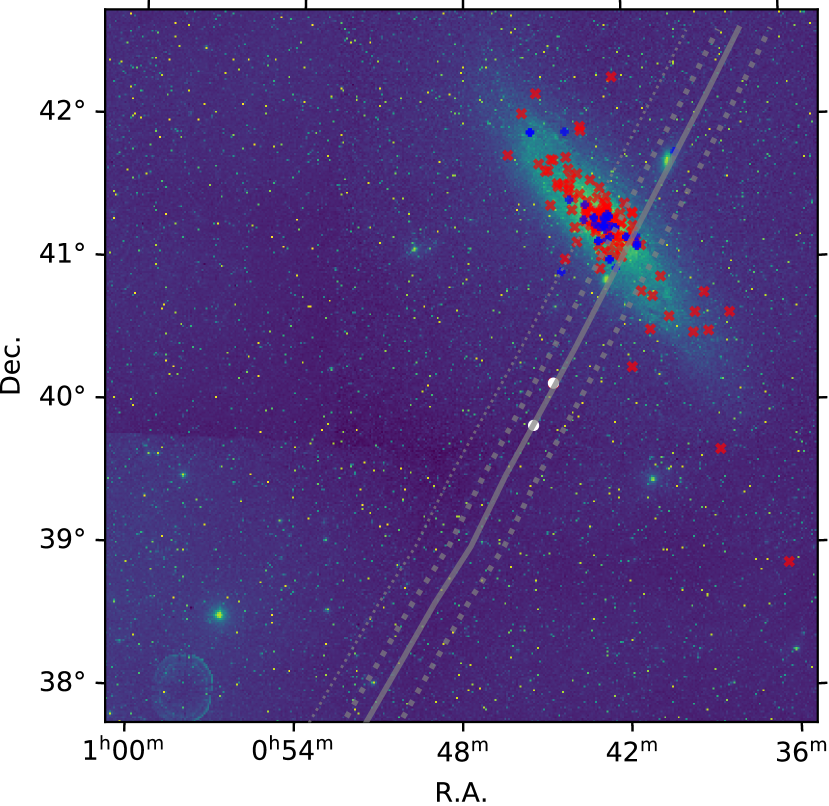
Figure 9: As Figure 1, but showing a much wider field, with M 31 offset to the north-west. The solid grey diagonal line indicated the approximate location of the peak stellar density of the M 31 Giant Stellar Stream, the dashed grey lines delimits the bulk of the stream’s stellar content, the dotted grey line indicates the lower density eastern confines of the stream. By inspection, AT 2016dah and AT 2017fyp clearly lie along the stream’s central peak density region.

The location of both AT 2016dah and AT 2017fyp along the line of the GSS (see Figure 9) strongly implies that the novae are physically located within the GSS, but with the spatial extent of surveys of M 31 and the substantial number of novae detected, it is important to consider the possibility that this alignment is a chance coincidence, and the novae are unconnected with the GSS.

4.1 Modelling the spatial distribution of a sample of novae

We therefore require a model for the underlying distribution of nova in our sample, assuming that the GSS is not a source of novae. Armed with such a model, we can create Monte Carlo (MC) simulations of the nova distribution and explore that fraction that have a similar (or greater) association to the GSS. We adopt the approach of Darnley et al. (2006) and Williams et al. (2016, also see , , and ) who define:

$$\Psi_{i}=\frac{\theta\mathscr{L}_{i}^{d}+\mathscr{L}_{i}^{b}}{\theta\sum_{i}\mathscr{L}_{i}^{d}+\sum_{i}\mathscr{L}_{i}^{b}},$$ (1)

where, over a grid of positions $i$, $\Psi$ is the probability of a nova erupting at a given location, $\theta$ is the ratio of the disk and bulge nova eruption rates per unit ($r^{\prime}$-band) flux, and $\mathscr{L}_{i}^{b}$ and $\mathscr{L}_{i}^{d}$ the disk and bulge contributions to the ($r^{\prime}$-band) flux at that location, respectively. Using this model Darnley et al. (2006) studied a sample of novae (see Darnley et al., 2004) close to the core of M 31 and found $\theta=0.18$. Williams et al. (2016) adopted the same value of $\theta$ but, with a larger, more heterogenous sample, they found that a correction needed to be applied to compensate for variable completeness of the sample.

To estimate the flux component $\mathscr{L}_{i}^{b}$ we model the bulge with elliptical isophotes with an axial ratio $b/a=0.6$ (Ciardullo et al., 1987) and a standard $r^{1/4}$ law (de Vaucouleurs, 1953). For the disk light $\mathscr{L}_{i}^{d}$, an exponential is used (Freeman, 1970). Both of these models are defined along the semi-major axis of the component ($a_{b}$ and $a_{d}$ for bulge and disk, respectively) yielding:

$$\log\left[{\mathscr{L}_{b}\left(a_{b}\right)/\mathscr{L}_{b}^{0}}\right]=-3.33\left[{\left({a_{b}/a_{b}^{0}}\right)^{1/4}-1}\right],$$ (2)

where $\mathscr{L}_{b}$ is the flux at some distance $a_{b}^{0}$ and is used for normalisation, and

$$\mathscr{L}_{d}(a_{d})=\mathscr{L}_{d}^{0}\,\mathrm{e}^{-a_{d}/a_{d}^{0}},$$ (3)

where $\mathscr{L}_{d}^{0}$ and $a_{d}^{0}$ are similarly normalisation factors.

We adopt a similar approach, but, clearly, require a different correction factor for our sample, which are the spectroscopically confirmed novae in the samples from Shafter et al. (2011) and C. Ransome et al. (in preparation), as shown in Figure 1. It is important to note that the purpose of this model is to produce suitable MC simulations that mirror the underlying constraints of the observed sample. There is a degeneracy between the specific value for $\theta$ used and the details of the completeness correction, so no conclusions can be drawn from the exact values of either, but as long as the observed distribution is matched, the MC simulations can be used to test the hypothesis that the GSS is not the source of any novae.

For each MC iteration, the model is used to create a probability of a nova occurring at any observed position in a fine grid, with a resolution of $4^{\prime\prime}$ over a large ($10^{\circ}\times 10^{\circ}$) field, and a random number generator used to seed a single nova. The simulated nova is associated at random to either the disk or bulge (weighted appropriately by the model flux values at that point) and a de-projected radius $r$ is calculated (i.e. the equivalent semi-major axis distance). The completion factor at that radius is then used to determine whether that particular nova is “observed” and placed into the mock catalogue for that iteration. This is repeated until the number of novae in the MC iteration matches the observed sample (276). This process is in turn repeated for a large number of MC iterations (at least 1000) to produce at least 1000 separate simulated nova “catalogues”.

For each MC iteration, a set of $r$ values for the observed nova are generated. Since the value of $r$ for a particular nova depends upon whether it is in the bulge or disk, and that is not known for the novae, the model is used to associate a probability of being bulge or disk with, for each MC iteration, every observed nova assigned at random in line with that probability and hence an appropriate $r$ calculated. Since the MC simulations only require us to produce a distribution with the correct radial characteristics, we do not need to estimate or model the full on-sky completeness function, but just correct for the incompleteness in $r$. Therefore, the completion correction is designed to minimise the difference between the cumulative distribution in $r$ of real and simulated nova. It was generated by taking the ratio of the cumulative distributions of uncorrected and observed nova in a series of bins in $\log(r)$ and fitting a set of steps to the ratio.

This can be seen in Figure 10 where the cumulative distribution in $r$ of the observed nova sample and combined MC iterations are compared. The correction factor comes in four steps: close to the core, completion is low; completion then increases out into the disk and is normalised to $1$ at its maximum before dropping down to a low level. This matches what might be expected. In the inner regions, the high background makes detection and spectroscopic follow-up of novae difficult, so as the flux from the galaxy drops, the completeness increases. However, further out coverage by surveys is less complete (particularly until recently, also see Section 5.6) and so completion drops again. However, it is important to remember that, although the form of the completion correction seems sensible, it is only used ensure that the model reproduces the observed distribution: a different value of $\theta$ would result in a different correction function, but the overall results would be largely unchanged.

Figure 10: Comparison of the spatial distribution model to the observed nova sample. Left: the cumulative distribution in $r$ of the observed novae (solid line) is compared to the equivalent distribution from a combination of 1000 MC iterations with a model value of $\theta=0.18$ (dashed line), without any completion correction. Right: the same observed distribution is compared to the result from MC simulations where the four-step correction function shown (thin, dotted line) is applied. A Kolmogorov (1933)–Smirnov (1948) test applied to the two sets of distributions gives a 0% chance that the uncorrected simulations are drawn from the observed distribution of novae, but a 67% chance that the corrected simulations are drawn from the observed distribution.

4.2 Modelling the Stream

McConnachie et al. (2003) provide a detailed description of the stellar light from the GSS, which can be used to produce a simplified model that we can apply to our observed nova sample and MC simulations. Our model follows the centre line of the GSS as determined by McConnachie et al. (2003, also see Figure 9), but approximates the light with a two-dimensional representation along the GSS.

At each position along the GSS (i.e. roughly perpendicular to the plane of M 31), and across the GSS, the average stellar light is given by the product of the simple form shown in Figure 11. It can be seen, however, that the component along the southern (negative distance) GSS rises sharply as it nears the plane of M 31. McConnachie et al. (2003) state that this excess is due to the GSS, and not contamination from the disk light, since it is not mirrored to the north. However, given that we are only concerned with the region where disk novae should be rare, we only consider the GSS more than $1^{\circ}$ from the plane of M 31. We also only consider the southern part of the GSS, giving the final GSS light model shown in Figure 12.

Figure 11: Our approximation to the GSS stellar light originally presented by McConnachie et al. (2003). On the left is simplified functional form we use to determine the average light along the GSS and on the right the equivalent across the GSS. The model light at any point is the product of the two functions at that position.

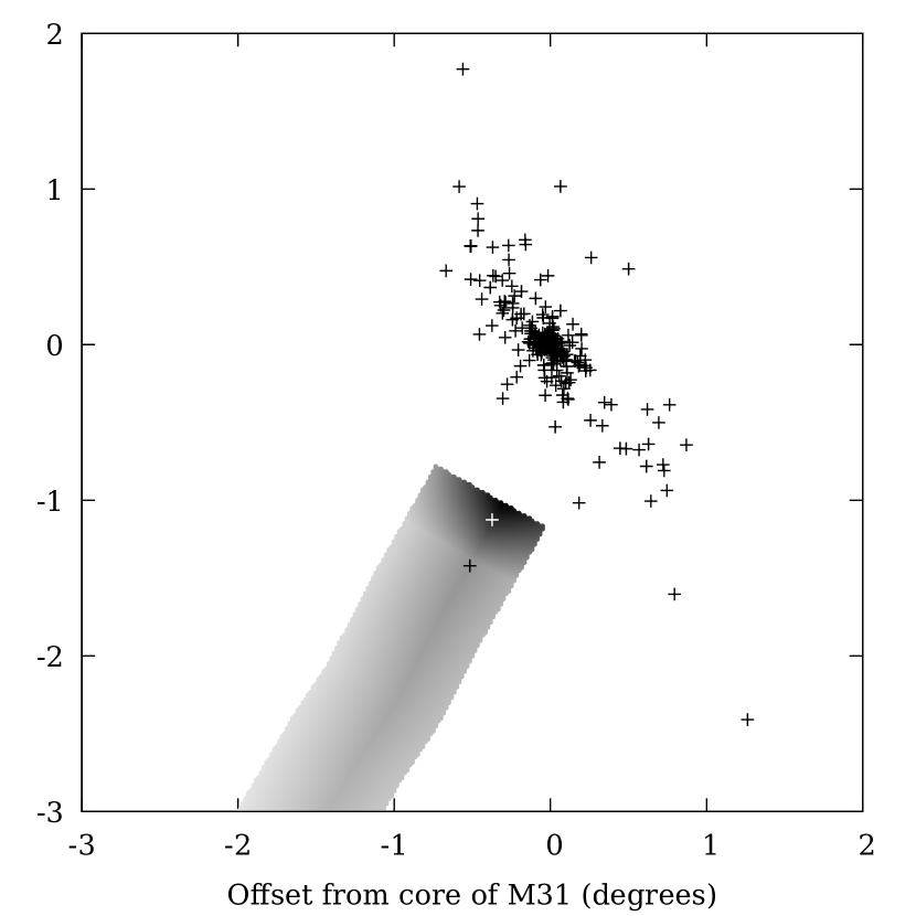
Figure 12: The simplified model of the Stream light used, with the sample of observed novae shown for comparison, cf. Figure 9.

Given this model, we can determine the association of GSS light with novae (observed or MC simulated) by summing the GSS light at the position of all novae in a given sample. Novae that fall outside the GSS will produce no contribution, while those that fall inside the GSS will contribute in proportion to the stellar light at that point. For the observed sample of novae, only AT 2016dah and AT 2017fyp contribute and so we use that value to normalise the result from the MC simulated samples. The result from 10,000 MC simulations of novae distributions is given in the histogram in Figure 13. Since the MC simulations only include the disk and bulge, any association with the GSS is random and so this gives an estimate of the likelihood that AT 2016dah and AT 2017fyp are coincidentally associated with the GSS.

Figure 13: The histogram of GSS light associated with novae in the MC simulations. GSS light is normalised to $1$ for the observed nova sample (i.e. AT 2016dah and AT 2017fyp). The inset shows the same histogram with the bin at zero GSS light removed. As can be seen, the majority of simulations have no novae on the GSS but there is a tail that stretches past $1$.

Although the majority of simulations have no GSS light associated with novae, 1.3% (132 out of 10,000 simulations) have normalised light greater than $1$ — in other words they have more GSS light associated with simulated novae than the light associated with the observed nova sample. As such, we can exclude the hypothesis that the GSS is not the source of AT 2016dah and AT 2017fyp at well beyond the $2\sigma$ confidence limit.

5 Discussion

As an aid to the reader, in Table 4 we provide a summary of key parameters for both AT 2016dah and 2017fyp.

Table 4: Summary of key parameters for AT 2016dah and AT 2017fyp.

Parameter	AT 2016dah	AT 2017fyp
R.A. (J2000)	$0^{\mathrm{h}}44^{\mathrm{m}}41^{\mathrm{s}}\!\!.05$	$0^{\mathrm{h}}45^{\mathrm{m}}25^{\mathrm{s}}\!\!.490$
Decl. (J2000)	$+40^{\circ}8^{\prime}35^{\prime\prime}\!\!.9$	$+39^{\circ}50^{\prime}52^{\prime\prime}\!\!.34$
Discovery date [UT]	2016 Jul 12	2017 Aug 7
Time of eruption [UT]	2016 Jul $11.96\pm 0.48$	2017 Aug $6.08\pm 1.48$
Strope, Schaefer & Henden (2010) light curve morphology	Smooth “S”	“S” or Flat topped “F”
Time of maximum [days post-eruption]	2.48	4–9
Peak observed apparent magnitude ($r^{\prime}$) [mag]	$16.32\pm 0.06$	$17.041\pm 0.007$
$r^{\prime}$-band $t_{2}$ / $t_{3}$ decline time [days]	$13.3^{+0.6}_{-0.3}$ / $26\pm 2$	32–37 / 63–68
$V$-band $t_{2}$ / $t_{3}$ decline time [days]	$7\pm 1$ / $13\pm 1$	16–21 / 38–43
$B$-band $t_{2}$ / $t_{3}$ decline time [days]	$8\pm 1$ / $16^{+3}_{-2}$	20–25 / 53-58
Payne-Gaposchkin (1964) speed class ($V$-band)	Very fast	Fast
Assumed reddening $E\left(B-V\right)$ [mag]	0.1	0.1
Williams (1992) spectral taxonomic class	Fe iib	Hybrid
Radial velocity (heliocentric corrected) [km s-1]	$-420\pm 30$	$-580\pm 50$
H$\alpha$ FWHM [km s-1]	$2300\pm 70$	$2550\pm 60$

5.1 AT 2016dah

With a $V$-band $t_{2}=7\pm 1$ d and exhibiting expansion velocities (inferred from the Balmer emission line FWHM and P Cygni terminal velocities) of 2300 km s^-1, this rapid evolution of AT 2016dah is at the extremes of those observed for Fe ii nova in M 31. In their photometric and spectroscopic survey of 48 new M 31 novae (91 in total), the fastest light curve evolution reported by Shafter et al. (2011) for an Fe ii nova was $t_{2}(V)=8.9\pm 0.2$ d for the luminous nova M31N 2009-10b. However, the H$\alpha$ line width of M31N 2009-10b only reached $\sim 1700$ km s^-1 (Barsukova et al., 2009; Di Mille et al., 2009). Indeed, none of the Fe ii novae reported by Shafter et al. (2011, see their Figure 16) displayed H$\alpha$ FWHMa $>2000$ km s^-1. Hybrid novae, those that simultaneously show elements of the He/N and Fe ii spectral classes, or evolve from one to another, are also referred to as Fe iib or ‘broad’ novae (see, for e.g., Della Valle & Livio, 1998). Similarly to AT 2016dah, M31N 2005-09b displayed Fe ii, Na D, and He i emission, although the FWHM was only $\approx 2000$ km s^-1, Shafter et al. (2011) classified this system as a Fe iib (when including the hybrid M31N 2006-10b, just 2 of 91 spectroscopically confirmed novae in M 31 at that time were hybrids or Fe iib novae). If we turn to M 33 for comparison, similarly to their M 31 work, Shafter et al. (2012) reported photometric and spectroscopic observations of eight novae in M 33. Three of those novae, M33N 2003-09a, 2010-10a, and 2010-11a were classified as Fe iib, with H$\alpha$ FWHM velocities of 2700, 4210, and 2610 km s^-1, respectively. Here, M33N 2003-09a and 2010-11a, which show similar velocities to AT 2016dah, displayed ‘typical’ Fe ii spectra, where 2010-10a (like AT 2017fyp) present elements of both Fe ii and He/N spectra – a hybrid. It should be noted that the spectral properties of the vast majority of the Shafter et al. (2011); Shafter et al. (2012) novae were derived from a single snap-shot spectrum taken at essentially random times during their early evolution. Without detailed spectral sequences, as were obtained for both AT 2016dah and AT 2017fyp, it is always possible that a single spectrum does not reveal the whole picture of the evolution of a given nova (particularly if the contextual information provided by a well sampled light curve is unavailable).

The Heliocentric recession velocity of AT 2016dah is $-420\pm 30$ km s^-1, this is formally inconsistent (at $4\sigma$) with the accepted Heliocentric recession velocity of M 31, $-300\pm 4$ km s^-1 (de Vaucouleurs et al., 1991). We will discuss the interpretation of this apparent discrepancy in Section 5.6.

Mooley et al. (2016) reported 15 GHz radio observations of AT 2016dah using the Arcminute Microkelvin Imager (AMI) Large Array $\sim 25$ d post-eruption. Those authors reported a $3\sigma$ upper limit of 102 $\mu$Jy or a spectral luminosity $<7.2\times 10^{22}$ erg s^-1 Hz.

5.2 AT 2017fyp

AT 2017fyp displays elements of both Fe ii and He/N spectra simultaneously throughout its early decline. There is no evidence, over the spectral time-series collected of a transition from one spectral type to the other, although it is possible that Fe ii would have been more dominant should earlier spectra have been available. Given the spectral development and a mean FWHM of $2550\pm 60$ km s^-1, AT 2017fyp is typical of a hybrid spectral type. As with the similar Fe iib systems, hybrids appear rare in the M 31 population ($\sim 2$%; Shafter et al., 2011), but appear possibly more common in younger stellar populations such as M 33 (Shafter et al., 2012).

The light curve of AT 2017fyp reveals a short lived, $\sim 5$ d, plateau. As such, we chose to classify AT 2017fyp as an ‘F’-type or flat-topped nova (after Strope et al., 2010). The definition of such novae from Strope et al. (2010) describes a flat-top that lasts 2–8 months, much longer than seen for AT 2017fyp, those authors also indicate that only a handful of Galactic novae are F-type. However, Strope et al. (2010) suggest that V2295 Ophiuchi, which exhibited a flat-top lasting $\sim 8$ d, may also fall into this class. The physical mechanism driving the flat-top phenomenon is still unclear.

AT 2017fyp shows an even greater discrepancy with the Heliocentric recession velocity of M 31 than AT 2016dah. The recession velocity of $-580\pm 50$ km s^-1 differs from that of M 31 beyond $5\sigma$. Again, this shall be discussed in Section 5.6.

5.3 Maximum magnitude—rate of decline

The maximum magnitude—rate of decline (MMRD; Mclaughlin, 1945) relationship has been employed for some time to estimate distances to Galactic and extragalactic novae. In recent years the validity of that relationship has been called into question by a number of authors (see, for e.g., Shara et al. 2017 and Schaefer 2018). However, Selvelli & Gilmozzi (2019) and, more recently, Della Valle & Izzo (2020, who performed a reanalysis of existing MMRD data) refute such claims. In either case, due to the inherent scatter, the MMRD is not a reliable distance indicator to individual novae (such as the subjects of this paper) and is strongest when used to estimate a distance toward a population of novae (see Darnley & Henze 2019 and Della Valle & Izzo 2020 for discussions regarding recurrent novae). The MMRD does not have the sensitivity to discriminate between individual novae in the GSS and those within M 31.

Here, we simply employ the MMRD to explore whether the luminosity and decline times of AT 2016dah and AT 2017fyp are typical of the M 31 population. Darnley et al. (2006) derived the only $r^{\prime}$-band MMRD for M 31 novae (see their Equation 3). Using the measured $r^{\prime}$-band $t_{2}$ times for AT 2016dah and AT 2017fyp, their MMRD would predict peak apparent magnitudes of $r^{\prime}=16.2$ and 16.8, respectively. Both these MMRD predictions agree well with our observations. Additionally, the MMRD indicates that both novae are indeed of a typical luminosity for their speed class, when compared with the global M 31 population.

5.4 X-ray emission (or lack thereof)

AT 2016dah was observed with the XRT onboard Swift at eleven epochs between $7\leq\Delta t\leq 87$ d post-eruption. AT 2017fyp was observed with the XRT at ten epochs between $19\leq\Delta t\leq 171$ d post-eruption. No X-ray photons were detected for either source, see Table 2. At the distance of (and column toward) M 31, the super-soft X-ray source (SSS) of nova eruptions are regularly detected (see, for e.g., Henze et al., 2010, 2011, 2014), although a good proportion have gone undetected despite available X-ray observations. Henze et al. (2014) observed correlations between optical and X-ray parameters for M 31 novae. These included the unveiling of the SSS ($t_{\mathrm{on}}$) with $t_{2}$ and the expansion velocity $v_{\mathrm{exp}}$, as estimated from optical spectra, and between the end of the SSS phase ($t_{\mathrm{off}}$) with $t_{\mathrm{on}}$.

Utilising Equation 6 from Henze et al. (2014), we estimate the epoch of $t_{\mathrm{on}}$ using our $r^{\prime}$-band estimates of $t_{2}$ to be: $t_{\mathrm{on}}=70\pm 20$ d and $150\pm 70$ d post-eruption for AT 2016dah, and AT 2017fyp, respectively. Based on the H$\alpha$ FWHM measurements, which is assumed to be representative of the expansion velocity, we estimate (using Equation 7 from Henze et al., 2014): $t_{\mathrm{on}}\lesssim 90$ d and $t_{\mathrm{on}}\lesssim 80$ d post-eruption for AT 2016dah, and AT 2017fyp, respectively. The estimates from both methods for AT 2016dah are consistent, but given the larger expansion velocity yet slower decline of AT 2017fyp those estimates differ notably. We similarly estimate $t_{\mathrm{off}}$ using Equation 4 from Henze et al. (2014) to be in the range: $100\lesssim t_{\mathrm{off}}\lesssim 350$ d for AT 2016dah, and $150\lesssim t_{\mathrm{off}}\lesssim 740$ d or $t_{\mathrm{off}}\lesssim 260$ d for AT 2017fyp for the $t_{2}$ and $v_{\mathrm{exp}}$ methods, respectively.

Additionally, the appearance of He ii 4686 Å in a nova spectrum can be an indication that part of the ejecta, or any surviving, or reformed, accretion structure is being directly illuminated by the SSS. As such, the appearance of He ii often accompanies the unveiling of the SSS. For AT 2016dah, He ii may have appeared as early as day 14 (but this could also be O ii emission), by day 41 the identification of He ii is clearer. For AT 2017fyp, He ii emission appears at day 55 post-eruption. Both these epochs are consistent with the estimates using the Henze et al. (2014) relations.

Therefore is seems clear that there is a good likelihood that the Swift observations did sample the SSS phase of both AT 2016dah and AT 2017fyp. However, the SSS luminosity of these systems was below the detection limits of those observations, implying SSS luminosities $L_{\mathrm{SSS}}\lesssim 2\times 10^{36}$ erg s^-1 (sampled between 0.3–10 keV). Other possibilities include the ejecta only becoming optically thin to X-rays after the SSSs had turned-off (i.e. formally $t_{\mathrm{on}}>t_{\mathrm{off}}$). Or that the SSSs turned-on after both Swift campaigns had ended, given the behaviour of the Henze et al. (2014) M 31 sample, this seems unlikely for such fast novae. Finally, $t_{\mathrm{off}}$ may have occurred before the first Swift observations, i.e. before day 7 and 18 post-eruption for AT 2016dah and AT 2017fyp, respectively. However, only two novae have exhibited SSS phases so short, the recurrent novae V745 Scorpii ($t_{\mathrm{off}}\sim 6$ days; Page et al., 2015) and M31N 2008-12a ($t_{\mathrm{off}}\sim 15$ days, but only for the peculiarly late and short 2016 eruption; Henze et al., 2018). Such short SSS phases are due to a TNR on the surface of a near-Chandrasekhar mass WD, the critical/ignition mass is low and the surface conditions particularly extreme. However, neither AT 2016dah or AT 2017fyp show any properties that would imply that they may be recurrent novae (for e.g., extremely fast light curve evolution, under-luminous eruptions, high ejection velocities, (post-maximum) light curve plateaus, ejecta deceleration, evolved donor, etc.; see the discussions within Pagnotta & Schaefer, 2014; Darnley, 2019).

5.5 Quiescent systems

Darnley et al. (2012) demonstrated that the evolutionary state of the donor in a nova system could be determined by the position of that quiescent nova on a colour-magnitude diagram. This technique is particularly sensitive for those systems with giant donors, where the donor dominates the emission from the optical through to the mid/far-IR (also see Evans et al., 2014) at quiescence. Darnley et al. (2014) demonstrated that at the distance of M 31 and M 33 all quiescent novae with red giant donors could be recovered, with sufficiently deep and high spatial resolution imaging. Williams et al. (2016) and particularly Darnley et al. (2017b) went on to show that the accretion disk of systems with high mass transfer rates were recoverable in the Local Group by utilising the near-UV.

In Figure 14 we show the regions around AT 2016dah and AT 2017fyp in the McConnachie et al. (2003) CFHT data. As is shown in these images, there are no detected sources within at least $1^{\prime\prime}$ of either nova. Photometry at the position of the nova in the CFHT data gives the following quiescent upper limits: AT 2016dah, $V>24.8$ mag and $I>24.3$ mag; AT 2017fyp, $V>24.5$ mag and $I>22.4$ mag. Although they provide the best UV coverage of location of the two novae, the GALEX data are not of sufficient depth or spatial resolution to be useful. At the distance of M 31, the Galactic red giant donor RNe V3890 Sagittarii and T Coronae Borealis would have $I$-band magnitudes of $\sim 21.5$ and $\sim 22.2$, respectively (Darnley et al., 2012). The depth of the CFHT data are, however, sufficient to rule out such luminous red giant donors for both these systems. Therefore it is most likely that the mass donor in both systems is a main sequence star, although we also cannot rule out sub-giant donors for either system.

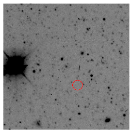
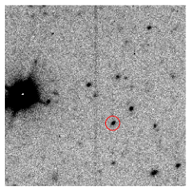
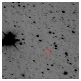
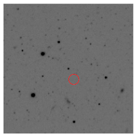
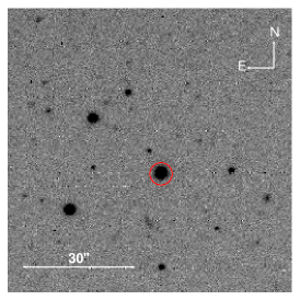
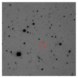
Figure 14: Progenitor search regions for AT 2016dah (top row) and AT 2017fyp (bottom row). The central image pair show Liverpool Telescope $r^{\prime}$-band eruption images ($3\times 180$ s exposure) with the erupting nova indicated by the red circle (radius $3^{\prime\prime}$). The images to the left and right show regions of the CFHT CFH12K mosaic data ($3\times 545$ s) around each nova (McConnachie et al., 2003), the nova position is again centred in the red circle; the left hand-image is $V$-band data, the right is $I$-band. All images are approximately a square arc-minute and have the same orientation, the image scale and orientation are indicated in the bottom-centre image. The CFHT data were not of sufficient depth to recover the progenitors systems (see text for details).

5.6 Giant Stellar Stream novae

Taken at face value, Figure 9, which shows the location of AT 2016dah and AT 2017fyp with respect to the GSS, is extremely suggestive that both novae should be strongly associated with the GSS. But upon further inspection, one does notice that there are a small number of other spectroscopically confirmed novae that appear beyond the bulk of the typical M 31 bulge–disk novae. Our analysis of the M 31 nova spatial distribution (see Section 4) does not definitively confirm that both AT 2016dah and AT 2017fyp are associated with the GSS. But it does indicate that the likelihood of, at least, two M 31 disk or bulge novae being spatially associated with the GSS by chance, at least as strongly as these two, is small, $\sim 1\%$.

Both AT 2016dah and AT 2017fyp reside within Field 7 of the CFHT targeted survey of the GSS undertaken by McConnachie et al. (2003). A radial velocity survey of the stream was reported by Ibata et al. (2004). That survey targeted four of the thirteen McConnachie et al. (2003) fields, unfortunately it did not cover field 7, but did survey fields 6 and 8, located either side of field 7. Ibata et al. (2004) reported a strong velocity gradient along the stream. The southern most tip has similar Heliocentric radial velocity to M 31 ($\sim-300$ km s^-1), whereas where the stream appears to coincide with M 31 it is approaching us relative to M 31 ($\sim-600$ km s^-1). The radial velocity within field 6 was $\sim-480$ km s^-1. As such, given the trend of radial velocity along the stream, we would expect the radial velocity of stream stars within field 7 to lie between -480 and -600 km s^-1. The radial velocity of AT 2016dah and AT 2017fyp are $-420\pm 30$ and $-580\pm 50$ km s^-1, respectively. Our radial velocity measurements will probably suffer from additional systematic uncertainties from, for e.g., the nova ejecta geometry, ejecta self-absorption, the low spectral resolution, and possibly even the binary orbital motion. Even so, these radial velocity measurements are strongly suggestive that both novae are members of the GSS.

Neither the spatial distribution analysis nor the radial velocity result alone provide the proverbial smoking gun. But, taken together they present compelling evidence for both AT 2016dah and AT 2017fyp to be considered members of the GSS and therefore not M 31 novae. As such, we will proceed under the assumption that both nova are associated with the GSS. But, with just two examples, it is hard to draw any concrete conclusions, nevertheless, one can speculate.

It is likely that the bulk of the stars associated with the GSS arose from the hitherto unidentified progenitor galaxy (see, e.g., Fardal et al., 2013; Kirihara et al., 2017; Hammer et al., 2018, and references therein). Therefore, it would seem probable that both AT 2016dah and AT 2017fyp were originally also part of the GSS progenitor. Recent simulations of the GSS formation have predicted that the progenitor was a small spiral galaxy (see, e.g., Fardal et al., 2013; Kirihara et al., 2017), perhaps not too unlike the present day M 33, although with a mass more akin to the Large Magellanic Cloud. As previously mentioned, Shafter et al. (2012) found significant differences between the spectroscopic properties of M 31 and M 33 novae. Fe iib and hybrid novae, such as AT 2016dah and AT 2017fyp, respectively, are rare among the M 31 population ($\sim 2\%$; Shafter et al., 2011); whereas such novae make up around half of those in M 33 (albeit it based on a sample of eight). However, the stellar mass of the GSS is substantially lower than M 33 or the LMC ($\sim 2.4\times 10^{8}$ M_⊙; Ibata et al., 2001a; Fardal et al., 2006), similar to that of the Local Group dwarf irregular NGC 6822 (Weldrake, de Blok & Walter, 2003). Based on the ‘Luminosity Specific Nova Rate’ (see Shafter et al., 2014; Darnley & Henze, 2019), the nova rate from such a stellar mass would be expected to be small: $\sim 0.1$ yr^-1.

We should therefore ask why have two GSS novae been discovered only a year apart? In part the answer to this lies in the history of nova (and all variable and transient) surveys in and around M 31. As discussed in Section 4, the completeness of the M 31 nova catalogue, particularly the spectroscopically confirmed catalogue, has both spatial and temporal dependence. M 31 nova survey strategy has (almost) always focussed on obtaining the largest amount of novae possible. In the early days, this meant focussing small fields on the bulge. As detector technology evolved, surveys expanded to cover more and more of the disk – but always with diminishing returns when considering the total nova yield (see Darnley & Henze, 2019, for a fuller discussion). In the past decade or so, high-cadence large-fields surveys – such as those employed here: ASAS-SN and PTF/iPTF/ZTF – have been able to probe the large volume around M 31, indeed the majority of the sky. So it is probably fair to say that we have only been capable of discovering (and confirming) GSS novae for around a decade. Given a nova rate of $\sim 0.1$ yr^-1, a yield of two novae in that time would be well within expectations. As the temporal baseline of the GSS (indeed all such streams in the Local Group) grows over the coming years and decades, we would expect to detect more such novae, and hopefully address some of the questions raised here.

6 Conclusions

In this Section we summarise the main findings of this paper.

1. The classical novae AT 2016dah and AT 2017fyp are located far to the south of the bulk of the content of M 31 and that host’s nova population.

2. AT 2016dah was discovered and followed photometrically and spectroscopically well before reaching maximum light. The initial spectra probe the fireball phase where the emission is dominated by a black body-like continuum.

3. AT 2016dah is a very fast nova with a S-type light curve that displays prominent Fe ii emission lines during its early decline. High ejecta velocities lead to a classification as a (rare for M 31) Fe iib nova.

4. AT 2017fyp was a fast nova, possibly with an F-type light curve, whose early decline spectra simultaneously contained Fe ii and He/N lines, leading to a classification as a hybrid nova.

5. Both novae were followed well into their nebular phase, in part aided by the low surface brightness so far from the centre of M 31.

6. Despite reasonable sampling by the Neil Gehrels Swift Observatory, the super-soft X-ray source of neither nova was detected. We propose that this is most likely due to the X-ray emission being below the detection limit of those observations.

7. A progenitor search within available archival data revealed no detected quiescent counterpart for either nova. We can rule out luminous red giant donors, cf. T CrB, and, as such, we suggest that both systems are most likely to harbour main sequence donors.

8. Hybrid and Fe iib novae are rare within the M 31 population, perviously accounting for just 2% of spectroscopically confirmed novae.

Both AT 2016dah and AT 2017fyp appear strongly associated with the Giant Stellar Stream to the south of M 31. The radial velocities of both novae imply an association with the GSS. The distribution of novae away from the bulge are elongated along the major axis of the inclined disk of M 31 and therefore are inconsistent with the broadly spherically-symmetric halo. However, our Monte Carlo simulations of the M 31 bulge and disk nova populations allows us to rule out a chance alignment of these two novae with the GSS at well beyond $2\sigma$. Combined, this evidence leads us to claim that both novae are associated with the GSS, indeed they are the first to be associated with any tidal stellar stream. Therefore, it would seem probable that these nova systems formed within the GSS progenitor galaxy and are therefore not associated with the M 31 nova population.

Appendix A Standards & Photometry — To appear on-line only

Table 5: Pan-STARRS sources used for calibration of the AT 2016dah photometry.

#	PANSTARRS ID	R.A. [J2000]	Dec. [J2000]	$u^{\prime}$ [mag]	$g$ [mag]	$r$ [mag]	$i$ [mag]	$z$ [mag]
001	156090110644167056	00:44:15.463	40:04:49.243	$17.656\pm 0.009$	$16.3037\pm 0.0033$	$15.8897\pm 0.0022$	$15.7505\pm 0.0029$	$15.7308\pm 0.0063$
002	156160110656529961	00:44:15.760	40:08:27.989	…	$17.9499\pm 0.0054$	$17.0009\pm 0.0028$	$16.5633\pm 0.0036$	$16.3556\pm 0.0055$
003	156130110677692991	00:44:16.260	40:06:37.018	…	$17.7762\pm 0.0032$	$16.5773\pm 0.0045$	$15.7959\pm 0.0033$	$15.4573\pm 0.0023$
004	156200110699024800	00:44:16.773	40:10:12.546	$18.554\pm 0.015$	$17.3553\pm 0.0038$	$16.9734\pm 0.0040$	$16.8323\pm 0.0019$	$16.8126\pm 0.0062$
005	156130110738743484	00:44:17.733	40:06:38.571	…	$17.2886\pm 0.0038$	$16.7190\pm 0.0024$	$16.4995\pm 0.0024$	$16.4233\pm 0.0046$
006	156200110751752256	00:44:18.039	40:10:04.912	$18.353\pm 0.013$	$17.1149\pm 0.0042$	$16.7029\pm 0.0021$	$16.5488\pm 0.0023$	$16.5033\pm 0.0050$
007	156210110791621242	00:44:18.996	40:10:31.895	…	$17.4554\pm 0.0046$	$16.7802\pm 0.0044$	$16.5194\pm 0.0023$	$16.4190\pm 0.0027$
008	156180110796444059	00:44:19.118	40:09:10.299	…	$17.4498\pm 0.0060$	$16.7872\pm 0.0016$	$16.5211\pm 0.0055$	$16.4331\pm 0.0022$
009	156120110839225356	00:44:20.143	40:06:14.152	…	$18.9666\pm 0.0074$	$17.8602\pm 0.0024$	$17.3163\pm 0.0030$	$17.0799\pm 0.0046$
010	156170110843570983	00:44:20.248	40:08:31.062	…	$18.4622\pm 0.0073$	$17.9648\pm 0.0031$	$17.7830\pm 0.0022$	$17.7251\pm 0.0130$
011	156100110880806753	00:44:21.142	40:05:18.355	…	$18.9225\pm 0.0037$	$18.1179\pm 0.0022$	$17.7768\pm 0.0034$	$17.6344\pm 0.0090$
012	156170110881700180	00:44:21.161	40:08:28.679	($18.023\pm 0.011$)	$16.7599\pm 0.0043$	$16.3255\pm 0.0030$	$16.1495\pm 0.0024$	$16.1035\pm 0.0040$
013	156170110937089548	00:44:22.491	40:08:56.767	…	$18.2470\pm 0.0045$	$17.8241\pm 0.0049$	$17.6634\pm 0.0031$	$17.6317\pm 0.0048$
014	156110110947737552	00:44:22.748	40:05:50.745	$17.474\pm 0.009$	$16.1101\pm 0.0032$	$15.7018\pm 0.0016$	$15.5640\pm 0.0014$	$15.5486\pm 0.0027$
015	156140110968363948	00:44:23.242	40:07:09.977	$18.521\pm 0.014$	$17.2107\pm 0.0032$	$16.8246\pm 0.0037$	$16.7036\pm 0.0032$	$16.6802\pm 0.0038$
016	156120110986003306	00:44:23.665	40:06:08.006	$17.625\pm 0.009$	$16.3398\pm 0.0045$	$15.9266\pm 0.0020$	$15.7504\pm 0.0033$	$15.7170\pm 0.0021$
017	156190111022894111	00:44:24.557	40:09:40.621	$17.376\pm 0.008$	$16.2472\pm 0.0016$	$15.8933\pm 0.0018$	$15.7477\pm 0.0012$	$15.7404\pm 0.0046$
018	156180111027502042	00:44:24.664	40:09:04.231	…	$17.7604\pm 0.0026$	$16.6848\pm 0.0037$	$16.1917\pm 0.0035$	$15.9631\pm 0.0038$
019	156270111030390210	00:44:24.734	40:13:28.853	$18.784\pm 0.017$	$16.4664\pm 0.0055$	$15.6159\pm 0.0208$	$15.2476\pm 0.0080$	$15.1235\pm 0.0328$
020	156180111061945695	00:44:25.481	40:09:15.163	…	$17.2991\pm 0.0048$	$16.0732\pm 0.0037$	$15.2836\pm 0.0011$	$14.9479\pm 0.0020$
021	156150111063803716	00:44:25.533	40:07:39.250	…	$18.9109\pm 0.0063$	$18.5321\pm 0.0043$	$18.3744\pm 0.0055$	$18.3251\pm 0.0068$
022	156250111084234164	00:44:26.024	40:12:40.610	…	$18.7826\pm 0.0095$	$17.9222\pm 0.0045$	$17.5841\pm 0.0029$	$17.4480\pm 0.0036$
023	156260111142147046	00:44:27.418	40:13:19.241	$18.250\pm 0.012$	$17.2940\pm 0.0058$	$16.9377\pm 0.0034$	$16.7916\pm 0.0019$	$16.7554\pm 0.0097$
024	156150111144823591	00:44:27.480	40:07:38.883	$17.716\pm 0.010$	$16.3153\pm 0.0035$	$15.8851\pm 0.0033$	$15.7374\pm 0.0030$	$15.7190\pm 0.0041$
025	156170111248306803	00:44:29.967	40:08:48.419	$16.577\pm 0.006$	$15.4359\pm 0.0049$	$15.0985\pm 0.0026$	$14.9342\pm 0.0057$	$14.9332\pm 0.0030$
026	156080111275685800	00:44:30.612	40:04:15.276	…	$18.9093\pm 0.0096$	$18.1147\pm 0.0052$	$17.8069\pm 0.0070$	$17.6719\pm 0.0063$
027	156200111355331018	00:44:32.527	40:10:01.064	$16.817\pm 0.007$	$15.2252\pm 0.0056$	$14.7269\pm 0.0020$	$14.5159\pm 0.0023$	$14.4667\pm 0.0045$
028	156160111365675490	00:44:32.777	40:08:14.647	…	$17.5087\pm 0.0059$	$16.7696\pm 0.0065$	$16.4292\pm 0.0027$	$16.3030\pm 0.0037$
029	156170111449725128	00:44:34.796	40:08:43.461	$18.985\pm 0.019$	$16.8984\pm 0.0052$	$16.1868\pm 0.0044$	$15.8379\pm 0.0030$	$15.7116\pm 0.0021$
030	156210111482725788	00:44:35.585	40:10:45.476	$18.557\pm 0.023$	$17.2055\pm 0.0018$	$16.7729\pm 0.0046$	$16.5986\pm 0.0043$	$16.5463\pm 0.0064$
031	156250111530102009	00:44:36.727	40:12:34.119	$17.081\pm 0.007$	$15.5910\pm 0.0036$	$15.1553\pm 0.0046$	$15.0231\pm 0.0020$	$14.9932\pm 0.0048$
032	156190111553904833	00:44:37.296	40:09:42.571	…	$18.1512\pm 0.0038$	$18.0010\pm 0.0064$	$17.9360\pm 0.0067$	$17.9725\pm 0.0056$
033	156130111559283525	00:44:37.425	40:06:38.660	…	$17.7247\pm 0.0056$	$17.3124\pm 0.0055$	$17.1426\pm 0.0042$	$17.1016\pm 0.0061$
034	156130111571613107	00:44:37.721	40:06:37.419	$17.988\pm 0.011$	$16.8690\pm 0.0061$	$16.5936\pm 0.0035$	$16.4917\pm 0.0034$	$16.5074\pm 0.0061$
035	156070111618596845	00:44:38.844	40:03:48.611	$17.980\pm 0.011$	$16.5189\pm 0.0017$	$16.0192\pm 0.0040$	$15.8272\pm 0.0035$	$15.7755\pm 0.0018$
036	156250111647920368	00:44:39.566	40:12:29.232	…	$18.9874\pm 0.0065$	$17.8149\pm 0.0030$	$16.5121\pm 0.0036$	$15.9213\pm 0.0025$
037	156240111671754193	00:44:40.122	40:12:10.677	…	$17.5945\pm 0.0031$	$16.9671\pm 0.0039$	$16.7421\pm 0.0033$	$16.6680\pm 0.0048$
038	156150111746426685	00:44:41.919	40:07:48.139	…	$18.2600\pm 0.0065$	$17.9116\pm 0.0067$	$17.7913\pm 0.0042$	$17.7706\pm 0.0061$
039	156070111814406664	00:44:43.551	40:03:48.107	…	$16.6669\pm 0.0041$	$15.6304\pm 0.0026$	$15.1438\pm 0.0020$	$14.9027\pm 0.0044$
040	156220111834228109	00:44:44.022	40:11:22.427	…	$17.3595\pm 0.0036$	$16.7560\pm 0.0029$	$16.4975\pm 0.0032$	$16.3980\pm 0.0058$
041	156100111856425487	00:44:44.559	40:05:14.551	…	$18.5278\pm 0.0049$	$18.1143\pm 0.0062$	$17.9701\pm 0.0043$	$17.9240\pm 0.0169$

Table 6: continued

Pan-STARRS sources used for calibration of the AT 2016dah photometry.

#	PANSTARRS ID	R.A. [J2000]	Dec. [J2000]	$u^{\prime}$ [mag]	$g$ [mag]	$r$ [mag]	$i$ [mag]	$z$ [mag]
042	156100111892817585	00:44:45.427	40:05:20.808	$17.199\pm 0.008$	$15.8041\pm 0.0057$	$15.3620\pm 0.0019$	$15.1845\pm 0.0025$	$15.1476\pm 0.0126$
043	156070111940992190	00:44:46.586	40:03:34.639	…	$18.3213\pm 0.0041$	$17.1903\pm 0.0037$	$16.6294\pm 0.0033$	$16.3634\pm 0.0010$
044	156140111960610721	00:44:47.060	40:07:00.256	$18.373\pm 0.013$	$16.9415\pm 0.0034$	$16.5210\pm 0.0066$	$16.3430\pm 0.0045$	$16.3010\pm 0.0065$
045	156220111972291992	00:44:47.337	40:11:04.077	…	$18.9742\pm 0.0050$	$17.8405\pm 0.0110$	$17.3388\pm 0.0050$	$17.0969\pm 0.0052$
046	156270111997920146	00:44:47.954	40:13:28.612	…	$18.8844\pm 0.0061$	$18.5681\pm 0.0078$	$18.4496\pm 0.0066$	$18.4517\pm 0.0103$
047	156180112021090440	00:44:48.507	40:08:59.410	…	$17.2182\pm 0.0031$	$16.6114\pm 0.0029$	$16.3756\pm 0.0031$	$16.2984\pm 0.0046$
048	156170112036494555	00:44:48.883	40:08:41.704	…	$17.7909\pm 0.0037$	$17.3121\pm 0.0048$	$17.1169\pm 0.0041$	$17.0537\pm 0.0062$
049	156140112044400367	00:44:49.074	40:06:59.142	($16.647\pm 0.006$)	$14.9905\pm 0.0051$	$14.4358\pm 0.0018$	$14.2234\pm 0.0040$	$14.1468\pm 0.0017$
050	156160112058941640	00:44:49.421	40:08:02.987	…	$18.2537\pm 0.0075$	$17.6608\pm 0.0030$	$17.4185\pm 0.0030$	$17.3486\pm 0.0010$
051	156140112064600997	00:44:49.554	40:07:01.108	…	$17.8526\pm 0.0284$	$17.4591\pm 0.0129$	$17.2538\pm 0.0141$	$16.9905\pm 0.0000$
052	156190112071334793	00:44:49.714	40:09:42.490	$17.103\pm 0.007$	$16.0337\pm 0.0042$	$15.7283\pm 0.0020$	$15.6207\pm 0.0028$	$15.6206\pm 0.0032$
053	156210112090386021	00:44:50.174	40:10:46.171	$18.419\pm 0.014$	$17.1505\pm 0.0042$	$16.7197\pm 0.0064$	$16.5693\pm 0.0037$	$16.5305\pm 0.0065$
054	156260112105642907	00:44:50.538	40:13:06.771	$18.814\pm 0.027$	$17.8051\pm 0.0036$	$17.4463\pm 0.0034$	$17.2856\pm 0.0034$	$17.2371\pm 0.0049$
055	156080112111492006	00:44:50.679	40:04:04.108	$18.867\pm 0.017$	$17.6831\pm 0.0065$	$17.3386\pm 0.0045$	$17.2115\pm 0.0044$	$17.1936\pm 0.0047$
056	156230112120840037	00:44:50.905	40:11:28.214	…	$17.9317\pm 0.0053$	$17.3185\pm 0.0065$	$17.0502\pm 0.0033$	$16.9520\pm 0.0031$
057	156220112125484788	00:44:51.013	40:11:12.472	…	$17.8751\pm 0.0089$	$17.2358\pm 0.0047$	$17.0000\pm 0.0044$	$16.9088\pm 0.0121$
058	156160112133718198	00:44:51.211	40:08:22.672	…	$18.7408\pm 0.0127$	$18.3304\pm 0.0144$	$17.9929\pm 0.0174$	$17.7062\pm 0.0375$
059	156150112237426105	00:44:53.694	40:07:46.533	$15.898\pm 0.005$	$14.7233\pm 0.0045$	$14.3935\pm 0.0043$	$14.2726\pm 0.0024$	$14.2762\pm 0.0011$
060	156230112264116066	00:44:54.338	40:11:46.334	…	$18.9226\pm 0.0058$	$18.3614\pm 0.0071$	$18.1427\pm 0.0037$	$18.0689\pm 0.0049$
061	156230112299867553	00:44:55.203	40:11:50.765	$18.320\pm 0.013$	$16.9859\pm 0.0066$	$16.5755\pm 0.0021$	$16.4268\pm 0.0038$	$16.4062\pm 0.0059$
062	156080112355827513	00:44:56.539	40:04:20.589	…	$17.0847\pm 0.0038$	$16.3731\pm 0.0030$	$16.0999\pm 0.0026$	$15.9926\pm 0.0036$
063	156230112419205551	00:44:58.064	40:11:44.771	$18.122\pm 0.012$	$16.8436\pm 0.0038$	$16.4434\pm 0.0025$	$16.2965\pm 0.0034$	$16.2764\pm 0.0123$
064	156120112421833902	00:44:58.129	40:06:09.748	($18.160\pm 0.012$)	$16.8911\pm 0.0024$	$16.4643\pm 0.0042$	$16.2820\pm 0.0024$	$16.2351\pm 0.0053$
065	156170112473351838	00:44:59.359	40:08:33.627	…	$16.8175\pm 0.0033$	$16.0500\pm 0.0021$	$15.7338\pm 0.0043$	$15.6020\pm 0.0039$
066	156240112515723853	00:45:00.380	40:12:09.643	…	$18.3057\pm 0.0047$	$17.4520\pm 0.0042$	$17.1155\pm 0.0028$	$16.9750\pm 0.0034$
067	156120112520510950	00:45:00.495	40:06:00.926	…	$18.5528\pm 0.0103$	$17.9829\pm 0.0058$	$17.7383\pm 0.0037$	$17.6381\pm 0.0053$
068	156120112577062471	00:45:01.847	40:06:05.454	…	$18.0864\pm 0.0037$	$17.7714\pm 0.0060$	$17.6525\pm 0.0029$	$17.6210\pm 0.0080$
069	156260112600944712	00:45:02.421	40:13:12.236	…	$18.7697\pm 0.0046$	$17.9717\pm 0.0029$	$17.6579\pm 0.0071$	$17.5353\pm 0.0038$
070	156240112615634528	00:45:02.777	40:12:11.679	…	$17.1378\pm 0.0030$	$16.5241\pm 0.0021$	$16.2635\pm 0.0027$	$16.1631\pm 0.0021$
071	156260112632996376	00:45:03.189	40:13:17.220	…	$18.9744\pm 0.0048$	$17.9458\pm 0.0038$	$17.4871\pm 0.0044$	$17.2691\pm 0.0037$
072	156170112653313107	00:45:03.684	40:08:37.408	$16.793\pm 0.007$	$15.5559\pm 0.0029$	$15.2125\pm 0.0060$	$15.0880\pm 0.0032$	$15.0924\pm 0.0042$
073	156150112654247660	00:45:03.705	40:07:51.097	…	$18.8042\pm 0.0051$	$17.6365\pm 0.0058$	$17.0592\pm 0.0038$	$16.8217\pm 0.0041$
074	156160112695481787	00:45:04.696	40:08:03.441	$18.916\pm 0.018$	$17.5036\pm 0.0076$	$17.0506\pm 0.0037$	$16.8692\pm 0.0032$	$16.8408\pm 0.0050$
075	156060112703737890	00:45:04.890	40:03:21.676	$16.502\pm 0.006$	$15.3819\pm 0.0045$	$15.0774\pm 0.0022$	$14.9836\pm 0.0028$	$14.9752\pm 0.0023$
076	156190112707227760	00:45:04.976	40:09:51.340	…	$17.4209\pm 0.0040$	$16.5761\pm 0.0025$	$16.2503\pm 0.0036$	$16.1257\pm 0.0047$
077	156180112722824341	00:45:05.363	40:09:10.709	…	$17.7212\pm 0.0033$	$16.4296\pm 0.0038$	$15.1527\pm 0.0035$	$14.5868\pm 0.0024$
078	156230112766257506	00:45:06.393	40:11:50.609	$18.514\pm 0.014$	$16.9715\pm 0.0057$	$16.4353\pm 0.0028$	$16.2072\pm 0.0029$	$16.1267\pm 0.0050$
079	156140112805430473	00:45:07.334	40:06:59.460	…	$18.9082\pm 0.0052$	$18.0323\pm 0.0043$	$17.6702\pm 0.0040$	$17.5090\pm 0.0057$
080	156110112841332677	00:45:08.194	40:05:36.093	…	$18.3729\pm 0.0041$	$17.6032\pm 0.0020$	$17.2863\pm 0.0037$	$17.1517\pm 0.0098$
081	156070112897527932	00:45:09.549	40:03:51.737	$16.513\pm 0.006$	$14.9578\pm 0.0019$	$14.5189\pm 0.0029$	$14.3702\pm 0.0017$	$14.3394\pm 0.0038$

Table 7: SDSS sources used for calibration of the AT 2017fyp photometry.

#	SDSS ID	R.A. [J2000]	Dec. [J2000]	$u^{\prime}$ [mag]	$g$ [mag]	$r$ [mag]	$i$ [mag]	$z$ [mag]
001	J004502.95+395457.1	00:45:02.960	39:54:57.139	$18.268\pm 0.013$	$17.159\pm 0.005$	$16.844\pm 0.005$	$16.723\pm 0.005$	$16.683\pm 0.009$
002	J004502.96+394717.8	00:45:02.967	39:47:17.826	$18.498\pm 0.019$	$16.936\pm 0.004$	$16.380\pm 0.004$	$16.316\pm 0.004$	$16.192\pm 0.008$
003	J004508.22+394731.5	00:45:08.220	39:47:31.546	$17.904\pm 0.014$	$16.350\pm 0.003$	$15.703\pm 0.003$	$15.582\pm 0.003$	$15.447\pm 0.005$
004	J004508.44+395313.0	00:45:08.444	39:53:13.038	$18.243\pm 0.017$	$17.034\pm 0.004$	$16.598\pm 0.004$	$16.382\pm 0.004$	$16.359\pm 0.008$
005	J004508.44+395312.9	00:45:08.447	39:53:12.991	$18.290\pm 0.013$	$17.051\pm 0.005$	$16.578\pm 0.004$	$16.408\pm 0.005$	$16.343\pm 0.008$
006	J004509.99+395522.6	00:45:09.999	39:55:22.681	$18.902\pm 0.026$	$17.539\pm 0.005$	$17.034\pm 0.004$	$16.753\pm 0.005$	$16.671\pm 0.011$
007	J004510.00+395522.7	00:45:10.003	39:55:22.721	$18.967\pm 0.018$	$17.559\pm 0.005$	$17.005\pm 0.005$	$16.795\pm 0.005$	$16.699\pm 0.009$
008	J004510.43+395257.2	00:45:10.439	39:52:57.245	$18.451\pm 0.019$	$17.315\pm 0.004$	$16.959\pm 0.004$	$16.764\pm 0.005$	$16.743\pm 0.011$
009	J004510.44+395257.1	00:45:10.443	39:52:57.173	$18.460\pm 0.014$	$17.319\pm 0.005$	$16.933\pm 0.005$	$16.782\pm 0.005$	$16.755\pm 0.009$
010	J004510.52+394700.9	00:45:10.520	39:47:00.906	$18.155\pm 0.016$	$16.286\pm 0.003$	$15.473\pm 0.003$	$15.285\pm 0.003$	$15.104\pm 0.004$
011	J004512.17+395339.0	00:45:12.179	39:53:39.001	$18.342\pm 0.018$	$17.201\pm 0.004$	$16.990\pm 0.004$	$16.843\pm 0.005$	$16.888\pm 0.012$
012	J004512.18+395338.9	00:45:12.183	39:53:38.933	$18.369\pm 0.013$	$17.218\pm 0.005$	$16.954\pm 0.005$	$16.877\pm 0.005$	$16.869\pm 0.010$
013	J004512.93+395424.2	00:45:12.935	39:54:24.296	$18.984\pm 0.019$	$17.937\pm 0.006$	$17.719\pm 0.006$	$17.664\pm 0.007$	$17.647\pm 0.016$
014	J004512.93+395424.4	00:45:12.936	39:54:24.437	$18.940\pm 0.027$	$17.896\pm 0.006$	$17.737\pm 0.006$	$17.564\pm 0.007$	$17.696\pm 0.022$
015	J004514.02+395155.0	00:45:14.028	39:51:55.051	$17.833\pm 0.010$	$15.520\pm 0.004$	$14.588\pm 0.004$	$14.267\pm 0.004$	$14.101\pm 0.004$
016	J004514.03+395155.1	00:45:14.039	39:51:55.102	$17.738\pm 0.013$	$15.525\pm 0.003$	$14.587\pm 0.003$	$14.252\pm 0.003$	$14.094\pm 0.003$
017	J004516.57+395054.1	00:45:16.580	39:50:54.168	$18.300\pm 0.017$	$17.161\pm 0.004$	$16.653\pm 0.004$	$16.452\pm 0.004$	$16.421\pm 0.009$
018	J004517.51+395017.2	00:45:17.511	39:50:17.290	$17.133\pm 0.009$	$16.049\pm 0.003$	$15.540\pm 0.003$	$15.396\pm 0.003$	$15.393\pm 0.005$
019	J004523.08+395417.6	00:45:23.088	39:54:17.629	$17.639\pm 0.012$	$16.000\pm 0.003$	$15.387\pm 0.003$	$15.233\pm 0.003$	$15.166\pm 0.005$
020	J004523.09+395417.5	00:45:23.091	39:54:17.590	$17.686\pm 0.010$	$15.962\pm 0.004$	$15.379\pm 0.004$	$15.211\pm 0.004$	$15.153\pm 0.005$
021	J004523.18+394929.4	00:45:23.184	39:49:29.402	$17.796\pm 0.013$	$16.383\pm 0.003$	$15.727\pm 0.003$	$15.520\pm 0.003$	$15.464\pm 0.005$
022	J004523.95+395257.0	00:45:23.953	39:52:57.011	$17.868\pm 0.014$	$16.641\pm 0.003$	$16.177\pm 0.003$	$15.970\pm 0.004$	$15.910\pm 0.007$
023	J004524.26+394604.0	00:45:24.263	39:46:04.048	$18.617\pm 0.021$	$17.050\pm 0.004$	$16.307\pm 0.004$	$16.156\pm 0.004$	$15.987\pm 0.007$
024	J004526.61+395151.8	00:45:26.611	39:51:51.811	$18.229\pm 0.017$	$16.359\pm 0.003$	$15.694\pm 0.003$	$15.437\pm 0.003$	$15.377\pm 0.005$
025	J004531.32+395120.7	00:45:31.326	39:51:20.801	$16.964\pm 0.008$	$15.745\pm 0.003$	$15.344\pm 0.003$	$15.165\pm 0.003$	$15.099\pm 0.005$
026	J004531.75+394710.2	00:45:31.751	39:47:10.277	$18.576\pm 0.020$	$17.462\pm 0.005$	$16.863\pm 0.004$	$16.708\pm 0.004$	$16.652\pm 0.010$
027	J004539.23+395519.7	00:45:39.230	39:55:19.733	$16.591\pm 0.007$	$15.532\pm 0.003$	$14.853\pm 0.003$	$14.869\pm 0.003$	$14.612\pm 0.004$
028	J004539.23+395150.7	00:45:39.234	39:51:50.785	$17.470\pm 0.011$	$16.348\pm 0.003$	$15.861\pm 0.003$	$15.683\pm 0.004$	$15.545\pm 0.006$
029	J004539.94+395310.7	00:45:39.948	39:53:10.795	$18.045\pm 0.016$	$16.819\pm 0.004$	$16.340\pm 0.003$	$16.115\pm 0.004$	$15.923\pm 0.007$
030	J004542.02+395540.1	00:45:42.029	39:55:40.102	$18.993\pm 0.029$	$17.728\pm 0.005$	$17.347\pm 0.005$	$17.022\pm 0.005$	$16.891\pm 0.012$
031	J004542.29+395356.0	00:45:42.297	39:53:56.011	$18.530\pm 0.021$	$17.328\pm 0.005$	$16.939\pm 0.004$	$16.686\pm 0.005$	$16.567\pm 0.010$
032	J004542.81+395446.3	00:45:42.812	39:54:46.372	$18.512\pm 0.021$	$17.362\pm 0.005$	$17.083\pm 0.004$	$16.832\pm 0.005$	$16.765\pm 0.011$
033	J004543.05+395330.1	00:45:43.058	39:53:30.196	$18.870\pm 0.027$	$17.360\pm 0.005$	$16.792\pm 0.004$	$16.485\pm 0.004$	$16.282\pm 0.008$
034	J004543.89+395208.7	00:45:43.894	39:52:08.796	$18.163\pm 0.017$	$16.087\pm 0.003$	$15.068\pm 0.003$	$14.900\pm 0.003$	$14.602\pm 0.004$
035	J004544.66+394854.3	00:45:44.670	39:48:54.349	$18.449\pm 0.019$	$17.137\pm 0.004$	$16.630\pm 0.004$	$16.374\pm 0.004$	$16.327\pm 0.008$
036	J004544.81+395228.5	00:45:44.818	39:52:28.564	$18.669\pm 0.023$	$17.366\pm 0.005$	$16.919\pm 0.004$	$16.668\pm 0.005$	$16.548\pm 0.010$
037	J004545.84+395159.0	00:45:45.848	39:51:59.008	$18.294\pm 0.019$	$16.478\pm 0.003$	$15.672\pm 0.003$	$15.483\pm 0.003$	$15.233\pm 0.005$
038	J004546.48+395124.4	00:45:46.482	39:51:24.433	$16.877\pm 0.008$	$15.842\pm 0.003$	$15.309\pm 0.003$	$15.254\pm 0.003$	$15.080\pm 0.005$
039	J004549.07+394615.8	00:45:49.076	39:46:15.888	$17.260\pm 0.010$	$15.928\pm 0.003$	$15.377\pm 0.003$	$15.183\pm 0.003$	$15.127\pm 0.005$
040	J004549.20+395351.2	00:45:49.200	39:53:51.259	$18.048\pm 0.016$	$17.025\pm 0.004$	$16.762\pm 0.004$	$16.573\pm 0.005$	$16.480\pm 0.010$
041	J004550.16+395505.2	00:45:50.162	39:55:05.243	$18.402\pm 0.020$	$16.259\pm 0.004$	$15.089\pm 0.003$	$14.884\pm 0.003$	$14.497\pm 0.004$
042	J004552.73+394907.4	00:45:52.733	39:49:07.428	$17.989\pm 0.015$	$15.952\pm 0.003$	$15.045\pm 0.003$	$14.805\pm 0.003$	$14.546\pm 0.004$

Table 8: Photometry of nova AT 2016dah as obtained by ASAS-SN (also see Nicolas et al., 2016), iPTF, and the LT.

Date	$\Delta t$	MJD $57000+$		Telescope and	Exposure	Filter	SNR	Photometry
[UT]	[days]	Start	End	Instrument	[s]			[mag]
2016 Jul 16.067	004.107	585.064	585.069	LT IO:O	$3\times 120$	$u^{\prime}$	119.0	$15.908\pm 0.048$
2016 Jul 17.069	005.109	586.067	586.072	LT IO:O	$3\times 120$	$u^{\prime}$	141.8	$16.254\pm 0.047$
2016 Jul 18.059	006.099	587.057	587.061	LT IO:O	$3\times 120$	$u^{\prime}$	68.5	$16.630\pm 0.048$
2016 Jul 19.055	007.095	588.052	588.057	LT IO:O	$3\times 120$	$u^{\prime}$	41.0	$16.960\pm 0.053$
2016 Jul 22.095	10.135	591.093	591.097	LT IO:O	$3\times 120$	$u^{\prime}$	65.9	$17.256\pm 0.051$
2016 Jul 25.050	13.090	594.047	594.052	LT IO:O	$3\times 120$	$u^{\prime}$	52.3	$17.551\pm 0.051$
2016 Jul 27.053	15.093	596.051	596.056	LT IO:O	$3\times 120$	$u^{\prime}$	20.8	$18.201\pm 0.073$
2016 Aug 03.123	22.163	603.121	603.125	LT IO:O	$3\times 120$	$u^{\prime}$	45.1	$18.513\pm 0.057$
2016 Aug 09.043	28.083	609.040	609.045	LT IO:O	$3\times 120$	$u^{\prime}$	14.8	$18.712\pm 0.117$
2016 Aug 17.047	36.087	617.045	617.050	LT IO:O	$3\times 120$	$u^{\prime}$	12.1	$19.479\pm 0.102$
2016 Aug 19.078	38.118	619.075	619.080	LT IO:O	$3\times 120$	$u^{\prime}$	9.1	$19.541\pm 0.130$
2016 Aug 21.108	40.148	621.106	621.110	LT IO:O	$3\times 120$	$u^{\prime}$	3.2	$18.315\pm 0.348$
2016 Aug 27.050	46.090	627.048	627.052	LT IO:O	$3\times 120$	$u^{\prime}$	13.3	$19.845\pm 0.099$
2016 Aug 29.113	48.153	629.111	629.116	LT IO:O	$3\times 120$	$u^{\prime}$	21.6	$19.793\pm 0.082$
2016 Sep 06.090	56.130	637.088	637.092	LT IO:O	$3\times 120$	$u^{\prime}$	15.6	$20.622\pm 0.084$
2016 Sep 13.982	64.022	644.980	644.984	LT IO:O	$3\times 120$	$u^{\prime}$	3.5	$20.801\pm 0.316$
2016 Sep 24.074	74.114	655.069	655.079	LT IO:O	$3\times 300$	$u^{\prime}$	9.1	$21.220\pm 0.132$
2016 Sep 28.092	78.132	659.087	659.098	LT IO:O	$3\times 300$	$u^{\prime}$	39.2	$19.655\pm 0.063$
2016 Dec 07.912	148.952	729.902	729.923	LT IO:O	$3\times 600$	$u^{\prime}$	5.4	$21.508\pm 0.209$
2016 Jul 16.072	4.112	585.069	585.074	LT IO:O	$3\times 120$	$B$	215.3	$17.160\pm 0.012$
2016 Jul 17.074	5.114	586.072	586.077	LT IO:O	$3\times 120$	$B$	201.7	$17.476\pm 0.011$
2016 Jul 18.064	6.104	587.062	587.066	LT IO:O	$3\times 120$	$B$	132.3	$17.768\pm 0.013$
2016 Jul 19.059	7.099	588.057	588.062	LT IO:O	$3\times 120$	$B$	76.2	$18.023\pm 0.018$
2016 Jul 22.100	10.140	591.098	591.102	LT IO:O	$3\times 120$	$B$	57.3	$18.504\pm 0.022$
2016 Jul 25.055	13.095	594.052	594.057	LT IO:O	$3\times 120$	$B$	86.9	$18.760\pm 0.017$
2016 Jul 27.058	15.098	596.056	596.061	LT IO:O	$3\times 120$	$B$	24.2	$19.472\pm 0.048$
2016 Aug 03.128	22.168	603.125	603.130	LT IO:O	$3\times 120$	$B$	82.9	$19.775\pm 0.018$
2016 Aug 09.048	28.088	609.045	609.050	LT IO:O	$3\times 120$	$B$	25.5	$20.225\pm 0.045$
2016 Aug 17.052	36.092	617.050	617.055	LT IO:O	$3\times 120$	$B$	24.6	$20.390\pm 0.045$
2016 Aug 19.083	38.123	619.080	619.085	LT IO:O	$3\times 120$	$B$	17.1	$20.664\pm 0.065$
2016 Aug 21.113	40.153	621.111	621.115	LT IO:O	$3\times 120$	$B$	—	$>18.9$
2016 Aug 27.055	46.095	627.053	627.057	LT IO:O	$3\times 120$	$B$	37.1	$21.152\pm 0.031$
2016 Aug 29.118	48.158	629.116	629.121	LT IO:O	$3\times 120$	$B$	44.9	$21.174\pm 0.027$
2016 Sep 06.095	56.135	637.093	637.097	LT IO:O	$3\times 120$	$B$	30.8	$21.538\pm 0.037$
2016 Sep 13.987	64.027	644.985	644.989	LT IO:O	$3\times 120$	$B$	9.4	$21.756\pm 0.117$
2016 Sep 24.085	74.125	655.080	655.091	LT IO:O	$3\times 300$	$B$	16.1	$22.154\pm 0.068$
2016 Sep 28.104	78.144	659.098	659.109	LT IO:O	$3\times 300$	$B$	26.0	$21.801\pm 0.043$
2016 Dec 07.934	148.974	729.923	729.944	LT IO:O	$3\times 600$	$B$	2.6	$(22.723\pm 0.425)$
2016 Jul 11.52	-0.44	…	…	ASAS-SN	$3\times 60$	$V$	…	$>17.0$
2016 Jul 13.52	1.56	…	…	ASAS-SN	$3\times 60$	$V$	…	$16.8\pm 0.2$
2016 Jul 13.52	1.56	…	…	ASAS-SN	$3\times 60$	$V$	…	$16.6\pm 0.2$
2016 Jul 13.52	1.56	…	…	ASAS-SN	$3\times 60$	$V$	…	$>16.8$
2016 Jul 14.54	2.58	…	…	ASAS-SN	$3\times 60$	$V$	…	$16.2\pm 0.1$
2016 Jul 14.54	2.58	…	…	ASAS-SN	$3\times 60$	$V$	…	$16.6\pm 0.2$
2016 Jul 14.54	2.58	…	…	ASAS-SN	$3\times 60$	$V$	…	$16.5\pm 0.2$
2016 Jul 16.077	4.117	585.074	585.079	LT IO:O	$3\times 120$	$V$	331.2	$16.939\pm 0.013$
2016 Jul 17.079	5.119	586.077	586.082	LT IO:O	$3\times 120$	$V$	314.3	$17.310\pm 0.013$
2016 Jul 17.59	5.63	…	…	ASAS-SN	$3\times 60$	$V$	…	$>16.8$
2016 Jul 18.069	6.109	587.067	587.071	LT IO:O	$3\times 120$	$V$	185.5	$17.631\pm 0.014$
2016 Jul 19.064	7.104	588.062	588.067	LT IO:O	$3\times 120$	$V$	133.8	$17.890\pm 0.015$
2016 Jul 22.105	10.145	591.103	591.107	LT IO:O	$3\times 120$	$V$	98.1	$18.297\pm 0.017$
2016 Jul 25.060	13.100	594.057	594.062	LT IO:O	$3\times 120$	$V$	96.7	$18.674\pm 0.018$
2016 Jul 27.063	15.103	596.061	596.066	LT IO:O	$3\times 120$	$V$	29.2	$19.317\pm 0.040$
2016 Aug 03.133	22.173	603.130	603.135	LT IO:O	$3\times 120$	$V$	81.8	$19.919\pm 0.019$
2016 Aug 09.053	28.093	609.050	609.055	LT IO:O	$3\times 120$	$V$	20.4	$20.443\pm 0.055$
2016 Aug 17.057	36.097	617.055	617.059	LT IO:O	$3\times 120$	$V$	23.0	$20.682\pm 0.049$
2016 Aug 19.087	38.127	619.085	619.090	LT IO:O	$3\times 120$	$V$	12.1	$20.748\pm 0.090$
2016 Aug 21.118	40.158	621.116	621.120	LT IO:O	$3\times 120$	$V$	—	$>19.8$
2016 Aug 27.060	46.100	627.058	627.062	LT IO:O	$3\times 120$	$V$	32.1	$21.397\pm 0.036$
2016 Aug 29.123	48.163	629.121	629.126	LT IO:O	$3\times 120$	$V$	35.5	$21.386\pm 0.033$

Table 9: continued

Photometry of nova AT 2016dah as obtained by ASAN-SN, iPTF, and the LT.

Date	$\Delta t$	MJD $57000+$		Telescope and	Exposure	Filter	SNR	Photometry
[UT]	[days]	Start	End	Instrument	[s]			[mag]
2016 Sep 06.100	56.140	637.098	637.102	LT IO:O	$3\times 120$	$V$	26.4	$21.646\pm 0.043$
2016 Sep 13.992	64.032	644.990	644.994	LT IO:O	$3\times 120$	$V$	8.2	$21.946\pm 0.133$
2016 Sep 24.097	74.137	655.091	655.102	LT IO:O	$3\times 300$	$V$	12.6	$22.057\pm 0.087$
2016 Sep 28.115	78.155	659.109	659.120	LT IO:O	$3\times 300$	$V$	22.1	$22.140\pm 0.051$
2016 Dec 07.955	148.995	729.945	729.966	LT IO:O	$3\times 600$	$V$	2.6	$(22.855\pm 0.419)$
2016 Aug 25.40		…	…	iPTF CFH12K		$g^{\prime}$	…	$>20.5$
2016 Aug 26.40		…	…	iPTF CFH12K		$g^{\prime}$	…	$21.1\pm 0.2$
2016 Jul 11.48	-0.48	…	…	iPTF CFH12K		$r^{\prime}$	…	$>21.171$
2016 Jul 12.44	0.48	…	…	iPTF CFH12K		$r^{\prime}$	…	$18.78\pm 0.07$
2016 Jul 12.46	0.50	…	…	iPTF CFH12K		$r^{\prime}$	…	$18.72\pm 0.07$
2016 Jul 13.47	1.51	…	…	iPTF CFH12K		$r^{\prime}$	…	$17.03\pm 0.06$
2016 Jul 13.49	1.53	…	…	iPTF CFH12K		$r^{\prime}$	…	$17.0\pm 0.1$
2016 Jul 14.44	2.48	…	…	iPTF CFH12K		$r^{\prime}$	…	$16.32\pm 0.06$
2016 Jul 14.47	2.51	…	…	iPTF CFH12K		$r^{\prime}$	…	$16.37\pm 0.07$
2016 Jul 15.43	3.47	…	…	iPTF CFH12K		$r^{\prime}$	…	$16.71\pm 0.07$
2016 Jul 15.47	3.51	…	…	iPTF CFH12K		$r^{\prime}$	…	$16.69\pm 0.07$
2016 Jul 16.082	4.122	585.079	585.084	LT IO:O	$3\times 120$	$r^{\prime}$	545.0	$16.876\pm 0.003$
2016 Jul 16.42	4.46	…	…	iPTF CFH12K		$r^{\prime}$	…	$16.97\pm 0.06$
2016 Jul 16.46	4.50	…	…	iPTF CFH12K		$r^{\prime}$	…	$16.97\pm 0.07$
2016 Jul 17.084	5.124	586.082	586.086	LT IO:O	$3\times 120$	$r^{\prime}$	550.5	$17.125\pm 0.002$
2016 Jul 17.42	5.46	…	…	iPTF CFH12K		$r^{\prime}$	…	$17.21\pm 0.09$
2016 Jul 18.074	6.114	587.072	587.076	LT IO:O	$3\times 120$	$r^{\prime}$	349.7	$17.304\pm 0.003$
2016 Jul 19.069	7.109	588.067	588.072	LT IO:O	$3\times 120$	$r^{\prime}$	394.6	$17.475\pm 0.003$
2016 Jul 22.110	10.150	591.108	591.112	LT IO:O	$3\times 120$	$r^{\prime}$	153.3	$17.807\pm 0.007$
2016 Jul 23.50	11.54	…	…	iPTF CFH12K		$r^{\prime}$	…	$18.0\pm 0.1$
2016 Jul 25.064	13.104	594.062	594.067	LT IO:O	$3\times 120$	$r^{\prime}$	207.4	$18.128\pm 0.006$
2016 Jul 26.48	14.52	…	…	iPTF CFH12K		$r^{\prime}$	…	$18.3\pm 0.01$
2016 Jul 27.068	15.108	596.066	596.071	LT IO:O	$3\times 120$	$r^{\prime}$	98.1	$18.362\pm 0.011$
2016 Jul 27.45	15.49	…	…	iPTF CFH12K		$r^{\prime}$	…	$18.33\pm 0.09$
2016 Jul 27.49	15.53	…	…	iPTF CFH12K		$r^{\prime}$	…	$18.43\pm 0.08$
2016 Jul 28.43	16.47	…	…	iPTF CFH12K		$r^{\prime}$	…	$18.40\pm 0.07$
2016 Jul 28.48	16.52	…	…	iPTF CFH12K		$r^{\prime}$	…	$18.47\pm 0.08$
2016 Jul 29.43	17.47	…	…	iPTF CFH12K		$r^{\prime}$	…	$18.58\pm 0.08$
2016 Jul 29.47	17.51	…	…	iPTF CFH12K		$r^{\prime}$	…	$18.55\pm 0.07$
2016 Jul 30.44	18.48	…	…	iPTF CFH12K		$r^{\prime}$	…	$18.68\pm 0.07$
2016 Jul 31.46	19.50	…	…	iPTF CFH12K		$r^{\prime}$	…	$18.67\pm 0.08$
2016 Aug 02.45	21.49	…	…	iPTF CFH12K		$r^{\prime}$	…	$18.77\pm 0.08$
2016 Aug 02.49	21.53	…	…	iPTF CFH12K		$r^{\prime}$	…	$18.71\pm 0.07$
2016 Aug 03.138	22.178	603.135	603.140	LT IO:O	$3\times 120$	$r^{\prime}$	241.9	$18.962\pm 0.005$
2016 Aug 03.46	22.50	…	…	iPTF CFH12K		$r^{\prime}$	…	$18.99\pm 0.07$
2016 Aug 03.49	22.53	…	…	iPTF CFH12K		$r^{\prime}$	…	$18.86\pm 0.08$
2016 Aug 04.45	23.49	…	…	iPTF CFH12K		$r^{\prime}$	…	$18.95\pm 0.08$
2016 Aug 04.49	23.53	…	…	iPTF CFH12K		$r^{\prime}$	…	$18.92\pm 0.08$
2016 Aug 05.46	24.50	…	…	iPTF CFH12K		$r^{\prime}$	…	$19.06\pm 0.08$
2016 Aug 05.49	24.53	…	…	iPTF CFH12K		$r^{\prime}$	…	$19.09\pm 0.08$
2016 Aug 06.44	25.48	…	…	iPTF CFH12K		$r^{\prime}$	…	$19.12\pm 0.08$
2016 Aug 06.48	25.52	…	…	iPTF CFH12K		$r^{\prime}$	…	$19.20\pm 0.07$
2016 Aug 07.45	26.49	…	…	iPTF CFH12K		$r^{\prime}$	…	$19.18\pm 0.08$
2016 Aug 07.49	26.53	…	…	iPTF CFH12K		$r^{\prime}$	…	$19.18\pm 0.07$
2016 Aug 08.43	27.47	…	…	iPTF CFH12K		$r^{\prime}$	…	$19.29\pm 0.07$
2016 Aug 08.48	27.52	…	…	iPTF CFH12K		$r^{\prime}$	…	$19.29\pm 0.07$
2016 Aug 09.058	28.098	609.055	609.060	LT IO:O	$3\times 120$	$r^{\prime}$	81.7	$19.451\pm 0.013$
2016 Aug 09.42	28.46	…	…	iPTF CFH12K		$r^{\prime}$	…	$19.34\pm 0.07$
2016 Aug 09.46	28.50	…	…	iPTF CFH12K		$r^{\prime}$	…	$19.42\pm 0.09$
2016 Aug 10.44	29.48	…	…	iPTF CFH12K		$r^{\prime}$	…	$19.53\pm 0.09$
2016 Aug 11.39	30.43	…	…	iPTF CFH12K		$r^{\prime}$	…	$19.50\pm 0.09$
2016 Aug 11.43	30.47	…	…	iPTF CFH12K		$r^{\prime}$	…	$19.44\pm 0.07$
2016 Aug 17.062	36.102	617.060	617.064	LT IO:O	$3\times 120$	$r^{\prime}$	61.6	$19.927\pm 0.018$
2016 Aug 19.092	38.132	619.090	619.095	LT IO:O	$3\times 120$	$r^{\prime}$	41.9	$20.116\pm 0.026$
2016 Aug 21.123	40.163	621.120	621.125	LT IO:O	$3\times 120$	$r^{\prime}$	7.7	$20.631\pm 0.140$

Table 10: continued

Photometry of nova AT 2016dah as obtained by ASAN-SN, iPTF, and the LT.

Date	$\Delta t$	MJD $57000+$		Telescope and	Exposure	Filter	SNR	Photometry
[UT]	[days]	Start	End	Instrument	[s]			[mag]
2016 Aug 27.065	46.105	627.063	627.067	LT IO:O	$3\times 120$	$r^{\prime}$	74.7	$20.791\pm 0.015$
2016 Aug 29.128	48.168	629.126	629.131	LT IO:O	$3\times 120$	$r^{\prime}$	58.1	$20.836\pm 0.019$
2016 Sep 06.105	56.145	637.103	637.107	LT IO:O	$3\times 120$	$r^{\prime}$	46.4	$21.342\pm 0.023$
2016 Sep 13.997	64.037	644.995	644.999	LT IO:O	$3\times 120$	$r^{\prime}$	11.3	$21.726\pm 0.096$
2016 Sep 24.108	74.148	655.102	655.113	LT IO:O	$3\times 300$	$r^{\prime}$	24.5	$21.966\pm 0.044$
2016 Sep 28.126	78.166	659.121	659.131	LT IO:O	$3\times 300$	$r^{\prime}$	26.2	$22.182\pm 0.042$
2016 Jul 16.087	4.127	585.084	585.089	LT IO:O	$3\times 120$	$i^{\prime}$	464.6	$16.801\pm 0.003$
2016 Jul 17.089	5.129	586.087	586.091	LT IO:O	$3\times 120$	$i^{\prime}$	469.7	$17.115\pm 0.003$
2016 Jul 18.079	6.119	587.077	587.081	LT IO:O	$3\times 120$	$i^{\prime}$	383.1	$17.415\pm 0.003$
2016 Jul 19.074	7.114	588.072	588.077	LT IO:O	$3\times 120$	$i^{\prime}$	350.8	$17.723\pm 0.003$
2016 Jul 22.115	10.155	591.113	591.117	LT IO:O	$3\times 120$	$i^{\prime}$	124.7	$18.145\pm 0.009$
2016 Jul 25.069	13.109	594.067	594.072	LT IO:O	$3\times 120$	$i^{\prime}$	129.8	$18.624\pm 0.009$
2016 Jul 27.073	15.113	596.071	596.076	LT IO:O	$3\times 120$	$i^{\prime}$	39.4	$19.134\pm 0.028$
2016 Aug 03.143	22.183	603.140	603.145	LT IO:O	$3\times 120$	$i^{\prime}$	83.4	$19.983\pm 0.013$
2016 Aug 09.063	28.103	609.060	609.065	LT IO:O	$3\times 120$	$i^{\prime}$	16.4	$20.527\pm 0.066$
2016 Aug 17.067	36.107	617.065	617.069	LT IO:O	$3\times 120$	$i^{\prime}$	24.1	$21.068\pm 0.045$
2016 Aug 19.097	38.137	619.095	619.100	LT IO:O	$3\times 120$	$i^{\prime}$	20.5	$21.176\pm 0.053$
2016 Aug 21.128	40.168	621.125	621.130	LT IO:O	$3\times 120$	$i^{\prime}$	3.3	$21.298\pm 0.331$
2016 Aug 27.070	46.110	627.068	627.072	LT IO:O	$3\times 120$	$i^{\prime}$	21.6	$21.976\pm 0.050$
2016 Aug 29.133	48.173	629.131	629.136	LT IO:O	$3\times 120$	$i^{\prime}$	16.3	$21.932\pm 0.067$
2016 Sep 06.110	56.150	637.108	637.112	LT IO:O	$3\times 120$	$i^{\prime}$	14.3	$22.436\pm 0.076$
2016 Sep 14.002	64.042	645.000	645.004	LT IO:O	$3\times 120$	$i^{\prime}$	7.0	$22.417\pm 0.155$
2016 Sep 24.119	74.159	655.114	655.124	LT IO:O	$3\times 300$	$i^{\prime}$	6.8	$22.864\pm 0.159$
2016 Sep 28.137	78.177	659.132	659.143	LT IO:O	$3\times 300$	$i^{\prime}$	9.5	$22.802\pm 0.115$

Table 11: Photometry of nova AT 2017fyp as obtained by the LT, LCO, Gaia, and ATLAS (see Tonry et al., 2017).

Date	$\Delta t$	MJD $57000+$		Telescope and	Exposure	Filter	SNR	Photometry
[UT]	[days]	Start	End	Instrument	[s]			[mag]
2017 Aug 10.115	005.035	976.112	976.117	LT IO:O	$3\times 120$	$u^{\prime}$	189.2	$17.250\pm 0.010$
2017 Aug 12.047	006.967	978.045	978.049	LT IO:O	$3\times 120$	$u^{\prime}$	182.5	$17.220\pm 0.011$
2017 Aug 14.106	009.026	980.104	980.108	LT IO:O	$3\times 120$	$u^{\prime}$	242.6	$17.101\pm 0.009$
2017 Aug 18.206	13.126	984.204	984.208	LT IO:O	$3\times 120$	$u^{\prime}$	205.1	$17.678\pm 0.009$
2017 Aug 20.213	15.133	986.211	986.216	LT IO:O	$3\times 120$	$u^{\prime}$	142.5	$17.894\pm 0.012$
2017 Aug 22.165	17.085	988.163	988.166	LT IO:O	$2\times 120$	$u^{\prime}$	13.6	$18.286\pm 0.082$
2017 Aug 23.137	18.057	989.135	989.139	LT IO:O	$3\times 120$	$u^{\prime}$	115.0	$18.179\pm 0.011$
2017 Aug 25.060	19.980	991.058	991.063	LT IO:O	$3\times 120$	$u^{\prime}$	93.7	$18.444\pm 0.014$
2017 Aug 30.202	25.122	996.199	996.204	LT IO:O	$3\times 120$	$u^{\prime}$	89.5	$18.783\pm 0.014$
2017 Sep 04.970	30.890	1001.968	1001.972	LT IO:O	$3\times 120$	$u^{\prime}$	36.5	$19.144\pm 0.031$
2017 Sep 08.147	34.067	1005.145	1005.149	LT IO:O	$3\times 120$	$u^{\prime}$	45.3	$19.233\pm 0.026$
2017 Sep 11.108	37.028	1008.106	1008.111	LT IO:O	$3\times 120$	$u^{\prime}$	58.6	$19.384\pm 0.021$
2017 Sep 16.070	41.990	1013.067	1013.072	LT IO:O	$3\times 120$	$u^{\prime}$	33.9	$19.565\pm 0.033$
2017 Sep 23.072	48.992	1020.070	1020.075	LT IO:O	$3\times 120$	$u^{\prime}$	18.2	$19.448\pm 0.061$
2017 Oct 27.983	53.903	1024.980	1024.985	LT IO:O	$3\times 120$	$u^{\prime}$	30.6	$19.812\pm 0.037$
2017 Oct 07.936	63.856	1034.933	1034.938	LT IO:O	$3\times 120$	$u^{\prime}$	34.3	$20.060\pm 0.033$
2017 Oct 19.955	75.875	1046.953	1046.958	LT IO:O	$3\times 120$	$u^{\prime}$	33.7	$20.355\pm 0.033$
2017 Oct 23.051	78.971	1050.049	1050.053	LT IO:O	$3\times 120$	$u^{\prime}$	21.2	$20.318\pm 0.052$
2017 Oct 28.080	84.000	1055.078	1055.082	LT IO:O	$3\times 120$	$u^{\prime}$	20.4	$20.501\pm 0.054$
2017 Dec 21.913	138.833	1109.909	1109.918	LT IO:O	$3\times 240$	$u^{\prime}$	32.4	$20.592\pm 0.035$
2017 Aug 09.463	004.383	975.460	975.465	LCO Spectral	$3\times 120$	$B$	79.9	$17.577\pm 0.022$
2017 Aug 10.120	005.040	976.117	976.122	LT IO:O	$3\times 120$	$B$	244.5	$17.569\pm 0.017$
2017 Aug 12.052	006.972	978.050	978.054	LT IO:O	$3\times 120$	$B$	281.2	$17.610\pm 0.017$
2017 Aug 12.515	007.435	978.513	978.517	LCO Spectral	$3\times 120$	$B$	82.1	$17.793\pm 0.023$
2017 Aug 14.111	009.031	980.108	980.113	LT IO:O	$3\times 120$	$B$	403.2	$17.476\pm 0.013$
2017 Aug 15.483	10.403	981.481	981.485	LCO Spectral	$3\times 120$	$B$	67.3	$18.024\pm 0.048$
2017 Aug 18.211	13.131	984.209	984.213	LT IO:O	$3\times 120$	$B$	259.9	$18.233\pm 0.015$
2017 Aug 20.218	15.138	986.216	986.221	LT IO:O	$3\times 120$	$B$	187.7	$18.434\pm 0.018$

Table 12: continued

Photometry of nova AT 2017fyp as obtained by the LT, LCO, Gaia, and ATLAS.

Date	$\Delta t$	MJD $57000+$		Telescope and	Exposure	Filter	SNR	Photometry
[UT]	[days]	Start	End	Instrument	[s]			[mag]
2017 Aug 23.142	18.062	989.140	989.144	LT IO:O	$3\times 120$	$B$	191.4	$18.713\pm 0.016$
2017 Aug 24.569	19.489	990.567	990.571	LT LCO Spectral	$3\times 120$	$B$	43.9	$18.958\pm 0.032$
2017 Aug 25.065	19.985	991.063	991.068	LT IO:O	$3\times 120$	$B$	157.3	$18.994\pm 0.018$
2017 Aug 30.207	25.127	996.204	996.209	LT IO:O	$3\times 120$	$B$	129.6	$19.320\pm 0.016$
2017 Sep 04.974	30.894	1001.973	1001.975	LT IO:O	$3\times 60$	$B$	28.5	$19.588\pm 0.041$
2017 Sep 08.151	34.071	1005.150	1005.152	LT IO:O	$3\times 60$	$B$	25.2	$19.768\pm 0.047$
2017 Sep 11.112	37.032	1008.111	1008.114	LT IO:O	$3\times 60$	$B$	50.2	$19.869\pm 0.026$
2017 Sep 16.073	41.993	1013.072	1013.075	LT IO:O	$3\times 60$	$B$	24.0	$20.056\pm 0.047$
2017 Sep 23.076	48.996	1020.075	1020.078	LT IO:O	$3\times 60$	$B$	15.9	$20.050\pm 0.070$
2017 Sep 27.987	53.907	1024.985	1024.988	LT IO:O	$3\times 60$	$B$	33.0	$20.342\pm 0.036$
2017 Oct 07.939	63.859	1034.938	1034.941	LT IO:O	$3\times 60$	$B$	23.9	$20.596\pm 0.047$
2017 Oct 19.959	75.879	1046.958	1046.960	LT IO:O	$3\times 60$	$B$	41.9	$20.688\pm 0.029$
2017 Oct 23.055	78.975	1050.054	1050.056	LT IO:O	$3\times 60$	$B$	23.3	$20.651\pm 0.048$
2017 Oct 28.084	84.004	1055.083	1055.085	LT IO:O	$3\times 60$	$B$	22.6	$20.972\pm 0.051$
2017 Dec 21.920	138.840	1109.918	1109.923	LT IO:O	$3\times 120$	$B$	007.9	$21.997\pm 0.138$
2017 Aug 09.468	004.388	975.465	975.470	LCO Spectral	$3\times 120$	$V$	118.2	$17.379\pm 0.010$
2017 Aug 10.124	005.044	976.122	976.127	LT IO:O	$3\times 120$	$V$	260.0	$17.462\pm 0.006$
2017 Aug 12.057	006.977	978.055	978.059	LT IO:O	$3\times 120$	$V$	281.8	$17.571\pm 0.005$
2017 Aug 12.520	007.440	978.517	978.522	LCO Spectral	$3\times 120$	$V$	101.5	$17.621\pm 0.011$
2017 Aug 14.116	009.036	980.113	980.118	LT IO:O	$3\times 120$	$V$	388.7	$17.474\pm 0.004$
2017 Aug 15.488	10.408	981.486	981.490	LCO Spectral	$3\times 120$	$V$	122.9	$17.917\pm 0.010$
2017 Aug 18.216	13.136	984.214	984.218	LT IO:O	$3\times 120$	$V$	287.4	$18.242\pm 0.005$
2017 Aug 20.223	15.143	986.221	986.226	LT IO:O	$3\times 120$	$V$	203.2	$18.458\pm 0.007$
2017 Aug 23.147	18.067	989.144	989.149	LT IO:O	$3\times 120$	$V$	166.5	$18.780\pm 0.007$
2017 Aug 24.574	19.494	990.572	990.576	LCO Spectral	$3\times 120$	$V$	52.6	$18.963\pm 0.021$
2017 Aug 25.070	19.990	991.068	991.073	LT IO:O	$3\times 120$	$V$	154.8	$19.104\pm 0.008$
2017 Aug 30.212	25.132	996.209	996.214	LT IO:O	$3\times 120$	$V$	87.3	$19.571\pm 0.013$
2017 Sep 04.977	30.897	1001.976	1001.978	LT IO:O	$3\times 60$	$V$	33.0	$19.803\pm 0.034$
2017 Sep 08.154	34.074	1005.152	1005.155	LT IO:O	$3\times 60$	$V$	19.1	$19.996\pm 0.057$
2017 Sep 11.115	37.035	1008.114	1008.117	LT IO:O	$3\times 60$	$V$	45.3	$20.165\pm 0.025$
2017 Sep 16.076	41.996	1013.075	1013.078	LT IO:O	$3\times 60$	$V$	25.4	$20.332\pm 0.043$
2017 Sep 23.079	48.999	1020.078	1020.080	LT IO:O	$3\times 60$	$V$	005.8	$20.548\pm 0.189$
2017 Sep 27.989	53.909	1024.988	1024.991	LT IO:O	$3\times 60$	$V$	27.9	$20.617\pm 0.039$
2017 Oct 07.942	63.982	1034.941	1034.944	LT IO:O	$3\times 60$	$V$	12.8	$21.168\pm 0.085$
2017 Oct 19.962	76.002	1046.961	1046.963	LT IO:O	$3\times 60$	$V$	26.3	$21.153\pm 0.042$
2017 Oct 23.058	79.098	1050.057	1050.059	LT IO:O	$3\times 60$	$V$	12.5	$20.945\pm 0.087$
2017 Oct 28.087	84.127	1055.085	1055.088	LT IO:O	$3\times 60$	$V$	10.7	$21.723\pm 0.101$
2017 Dec 21.925	138.965	1109.923	1109.928	LT IO:O	$3\times 120$	$V$	004.0	$21.614\pm 0.274$
2017 Aug 24.006	17.926	…	…	Gaia	60	$G$	…	$17.92\pm 0.2$
2017 Sep 07.183	33.103	…	…	Gaia	60	$G$	…	$19.08$
2017 Sep 09.257	35.177	…	…	Gaia	60	$G$	…	$19.09$
2017 Aug 04.603	-1.475	…	…	ATLAS1 ACAM1	30	orange	—	$>19.28$
2017 Aug 07.553	1.475	…	…	ATLAS1 ACAM1	30	orange	…	$16.77\pm 0.09$
2017 Aug 09.473	004.393	975.470	975.475	LCO Spectral	$3\times 120$	$r^{\prime}$	195.2	$17.041\pm 0.007$
2017 Aug 10.129	005.049	976.127	976.132	LT IO:O	$3\times 120$	$r^{\prime}$	414.4	$17.092\pm 0.005$
2017 Aug 12.062	006.982	978.060	978.064	LT IO:O	$3\times 120$	$r^{\prime}$	452.0	$17.072\pm 0.004$
2017 Aug 12.525	007.445	978.522	978.527	LCO Spectral	$3\times 120$	$r^{\prime}$	249.2	$17.061\pm 0.005$
2017 Aug 14.121	009.041	980.118	980.123	LT IO:O	$3\times 120$	$r^{\prime}$	586.3	$16.974\pm 0.004$
2017 Aug 15.493	10.413	981.491	981.495	LCO Spectral	$3\times 120$	$r^{\prime}$	276.3	$17.155\pm 0.005$
2017 Aug 18.221	13.141	984.219	984.223	LT IO:O	$3\times 120$	$r^{\prime}$	611.3	$17.255\pm 0.007$
2017 Aug 20.228	15.148	986.226	986.230	LT IO:O	$3\times 120$	$r^{\prime}$	486.7	$17.288\pm 0.005$
2017 Aug 23.152	18.072	989.149	989.154	LT IO:O	$3\times 120$	$r^{\prime}$	489.6	$17.530\pm 0.004$
2017 Aug 24.579	19.499	990.577	990.581	LCO Spectral	$3\times 120$	$r^{\prime}$	191.0	$17.670\pm 0.006$
2017 Aug 25.075	19.995	991.073	991.078	LT IO:O	$3\times 120$	$r^{\prime}$	422.0	$17.736\pm 0.006$
2017 Aug 30.217	25.137	996.214	996.219	LT IO:O	$3\times 120$	$r^{\prime}$	324.4	$18.149\pm 0.005$
2017 Sep 04.980	30.900	1001.979	1001.981	LT IO:O	$3\times 60$	$r^{\prime}$	143.6	$18.460\pm 0.008$
2017 Sep 08.157	34.077	1005.155	1005.158	LT IO:O	$3\times 60$	$r^{\prime}$	81.1	$18.600\pm 0.014$
2017 Sep 11.118	37.038	1008.117	1008.119	LT IO:O	$3\times 60$	$r^{\prime}$	172.1	$18.783\pm 0.007$
2017 Sep 16.079	41.999	1013.078	1013.081	LT IO:O	$3\times 60$	$r^{\prime}$	98.6	$19.014\pm 0.011$

Table 13: continued

Photometry of nova AT 2017fyp as obtained by the LT, LCO, Gaia, and ATLAS.

Date	$\Delta t$	MJD $57000+$		Telescope and	Exposure	Filter	SNR	Photometry
[UT]	[days]	Start	End	Instrument	[s]			[mag]
2017 Sep 23.082	49.002	1020.081	1020.083	LT IO:O	$3\times 60$	$r^{\prime}$	17.0	$19.099\pm 0.064$
2017 Sep 27.992	53.912	1024.991	1024.994	LT IO:O	$3\times 60$	$r^{\prime}$	94.2	$19.438\pm 0.012$
2017 Oct 07.945	63.865	1034.944	1034.946	LT IO:O	$3\times 60$	$r^{\prime}$	56.5	$19.806\pm 0.019$
2017 Oct 23.061	78.981	1050.060	1050.062	LT IO:O	$3\times 60$	$r^{\prime}$	36.8	$20.162\pm 0.030$
2017 Oct 28.090	84.010	1055.088	1055.091	LT IO:O	$3\times 60$	$r^{\prime}$	42.1	$20.373\pm 0.026$
2017 Dec 21.929	138.849	1109.928	1109.931	LT IO:O	$3\times 60$	$r^{\prime}$	—	$>19.4$
2017 Aug 09.477	004.397	975.475	975.480	LCO Spectral	$3\times 120$	$i^{\prime}$	139.9	$17.147\pm 0.011$
2017 Aug 10.134	005.054	976.132	976.137	LT IO:O	$3\times 120$	$i^{\prime}$	327.8	$17.238\pm 0.012$
2017 Aug 12.067	006.987	978.065	978.069	LT IO:O	$3\times 120$	$i^{\prime}$	416.5	$17.337\pm 0.010$
2017 Aug 12.530	007.450	978.527	978.532	LCO Spectral	$3\times 120$	$i^{\prime}$	160.6	$17.386\pm 0.011$
2017 Aug 14.126	009.046	980.123	980.128	LT IO:O	$3\times 120$	$i^{\prime}$	427.9	$17.323\pm 0.015$
2017 Aug 15.498	10.418	981.496	981.500	LCO Spectral	$3\times 120$	$i^{\prime}$	194.9	$17.623\pm 0.010$
2017 Aug 18.226	13.146	984.224	984.228	LT IO:O	$3\times 120$	$i^{\prime}$	374.6	$17.864\pm 0.013$
2017 Aug 20.233	15.153	986.231	986.235	LT IO:O	$3\times 120$	$i^{\prime}$	230.8	$18.014\pm 0.016$
2017 Aug 23.157	18.077	989.154	989.159	LT IO:O	$3\times 120$	$i^{\prime}$	267.7	$18.385\pm 0.014$
2017 Aug 24.584	19.504	990.581	990.586	LCO Spectral	$3\times 120$	$i^{\prime}$	67.2	$18.635\pm 0.017$
2017 Aug 25.080	20.000	991.078	991.083	LT IO:O	$3\times 120$	$i^{\prime}$	188.0	$18.685\pm 0.012$
2017 Aug 30.222	25.142	996.219	996.224	LT IO:O	$3\times 120$	$i^{\prime}$	112.9	$19.230\pm 0.014$
2017 Sep 04.983	30.903	1001.981	1001.984	LT IO:O	$3\times 60$	$i^{\prime}$	52.0	$19.651\pm 0.024$
2017 Sep 08.159	34.079	1005.158	1005.161	LT IO:O	$3\times 60$	$i^{\prime}$	31.6	$19.679\pm 0.036$
2017 Sep 11.121	37.041	1008.120	1008.122	LT IO:O	$3\times 60$	$i^{\prime}$	57.6	$19.907\pm 0.021$
2017 Sep 16.082	42.002	1013.081	1013.083	LT IO:O	$3\times 60$	$i^{\prime}$	36.0	$20.185\pm 0.031$
2017 Sep 24.085	49.005	1020.084	1020.086	LT IO:O	$3\times 60$	$i^{\prime}$	16.7	$20.202\pm 0.065$
2017 Sep 27.995	53.915	1024.994	1024.996	LT IO:O	$3\times 60$	$i^{\prime}$	37.5	$20.626\pm 0.032$
2017 Oct 07.948	63.868	1034.947	1034.949	LT IO:O	$3\times 60$	$i^{\prime}$	19.1	$21.003\pm 0.058$
2017 Oct 23.064	78.984	1050.062	1050.065	LT IO:O	$3\times 60$	$i^{\prime}$	16.6	$21.172\pm 0.067$
2017 Oct 28.093	84.013	1055.091	1055.094	LT IO:O	$3\times 60$	$i^{\prime}$	12.2	$21.510\pm 0.090$
2017 Dec 21.932	138.852	1109.931	1109.933	LT IO:O	$3\times 60$	$i^{\prime}$	002.6	($21.462\pm 0.426$)

References

- Alam et al. (2015) Alam S., et al., 2015, ApJS, 219, 12
- Barnsley et al. (2012) Barnsley R. M., Smith R. J., Steele I. A., 2012, Astronomische Nachrichten, 333, 101
- Barsukova et al. (2009) Barsukova E., Afanasiev V., Fabrika S., Valeev A., Hornoch K., Pietsch W., 2009, The Astronomer’s Telegram, 2251, 1
- Bochanski et al. (2014) Bochanski J. J., Willman B., West A. A., Strader J., Chomiuk L., 2014, AJ, 147, 76
- Bode & Evans (2008) Bode M. F., Evans A., eds, 2008, Classical Novae, 2nd Edition. Cambridge Astrophysics Series Vol. 43, Cambridge University Press, Cambridge
- Bode et al. (2009) Bode M. F., Darnley M. J., Shafter A. W., Page K. L., Smirnova O., Anupama G. C., Hilton T., 2009, ApJ, 705, 1056
- Brown et al. (2013) Brown T. M., et al., 2013, PASP, 125, 1031
- Burrows et al. (2005) Burrows D. N., et al., 2005, Space Sci. Rev., 120, 165
- Cao et al. (2016) Cao Y., Nugent P. E., Kasliwal M. M., 2016, PASP, 128, 114502
- Chambers et al. (2016) Chambers K. C., et al., 2016, arXiv e-prints, p. arXiv:1612.05560
- Chinetti et al. (2016a) Chinetti K., Darnley M. J., Kasliwal M. M., Mazzali P., Neill J. D., Williams S. C., 2016a, The Astronomer’s Telegram, 9248
- Chinetti et al. (2016b) Chinetti K., Darnley M. J., Page K. L., Williams S. C., 2016b, The Astronomer’s Telegram, 9329
- Ciardullo et al. (1987) Ciardullo R., Ford H. C., Neill J. D., Jacoby G. H., Shafter A. W., 1987, ApJ, 318, 520
- Cuillandre et al. (2000) Cuillandre J.-C., Luppino G. A., Starr B. M., Isani S., 2000, in Iye M., Moorwood A. F., eds, Society of Photo-Optical Instrumentation Engineers (SPIE) Conference Series Vol. 4008, Proc. SPIE. pp 1010–1021, doi:10.1117/12.395465
- D’Onghia & Fox (2016) D’Onghia E., Fox A. J., 2016, ARA&A, 54, 363
- Dalcanton et al. (2015) Dalcanton J. J., et al., 2015, ApJ, 814, 3
- Darnley (2019) Darnley M. J., 2019, arXiv e-prints, p. arXiv:1912.13209
- Darnley & Henze (2019) Darnley M. J., Henze M., 2019, arXiv e-prints, p. arXiv:1909.10497
- Darnley et al. (2004) Darnley M. J., et al., 2004, MNRAS, 353, 571
- Darnley et al. (2006) Darnley M. J., et al., 2006, MNRAS, 369, 257
- Darnley et al. (2007) Darnley M. J., et al., 2007, ApJ, 661, L45
- Darnley et al. (2012) Darnley M. J., Ribeiro V. A. R. M., Bode M. F., Hounsell R. A., Williams R. P., 2012, ApJ, 746, 61
- Darnley et al. (2014) Darnley M. J., et al., 2014, in Woudt P. A., Ribeiro V. A. R. M., eds, Astronomical Society of the Pacific Conference Series Vol. 490, Stellar Novae: Past and Future Decades. p. 49 (arXiv:1303.2711)
- Darnley et al. (2016) Darnley M. J., et al., 2016, ApJ, 833, 149
- Darnley et al. (2017a) Darnley M. J., et al., 2017a, ApJ, 847, 35
- Darnley et al. (2017b) Darnley M. J., et al., 2017b, ApJ, 849, 96
- Della Valle & Izzo (2020) Della Valle M., Izzo L., 2020, arXiv e-prints, p. arXiv:2004.06540
- Della Valle & Livio (1998) Della Valle M., Livio M., 1998, ApJ, 506, 818
- Di Mille et al. (2009) Di Mille F., et al., 2009, The Astronomer’s Telegram, 2248, 1
- Dressler (1984) Dressler A., 1984, ARA&A, 22, 185
- Evans et al. (2009) Evans P. A., et al., 2009, MNRAS, 397, 1177
- Evans et al. (2014) Evans A., Gehrz R. D., Woodward C. E., Helton L. A., 2014, MNRAS, 444, 1683
- Fardal et al. (2006) Fardal M. A., Babul A., Geehan J. J., Guhathakurta P., 2006, MNRAS, 366, 1012
- Fardal et al. (2013) Fardal M. A., et al., 2013, MNRAS, 434, 2779
- Feldmeier et al. (1998) Feldmeier J. J., Ciardullo R., Jacoby G. H., 1998, ApJ, 503, 109
- Ferguson et al. (2002) Ferguson A. M. N., Irwin M. J., Ibata R. A., Lewis G. F., Tanvir N. R., 2002, AJ, 124, 1452
- Font et al. (2006) Font A. S., Johnston K. V., Guhathakurta P., Majewski S. R., Rich R. M., 2006, AJ, 131, 1436
- Freedman et al. (2001) Freedman W. L., et al., 2001, ApJ, 553, 47
- Freeman (1970) Freeman K., 1970, ApJ, 160, 811
- Gal-Yam et al. (2003) Gal-Yam A., Maoz D., Guhathakurta P., Filippenko A. V., 2003, AJ, 125, 1087
- Gehrels et al. (2004) Gehrels N., et al., 2004, ApJ, 611, 1005
- Gerhard et al. (2005) Gerhard O., Arnaboldi M., Freeman K. C., Kashikawa N., Okamura S., Yasuda N., 2005, ApJ, 621, L93
- Graham et al. (2015) Graham M. L., Sand D. J., Zaritsky D., Pritchet C. J., 2015, ApJ, 807, 83
- Güver & Özel (2009) Güver T., Özel F., 2009, MNRAS, 400, 2050
- HI4PI Collaboration et al. (2016) HI4PI Collaboration et al., 2016, A&A, 594, A116
- Hachisu & Kato (2006) Hachisu I., Kato M., 2006, ApJS, 167, 59
- Hammer et al. (2018) Hammer F., Yang Y. B., Wang J. L., Ibata R., Flores H., Puech M., 2018, MNRAS, 475, 2754
- Harvey et al. (2018) Harvey E. J., Redman M. P., Darnley M. J., Williams S. C., Berdyugin A., Piirola V. E., Fitzgerald K. P., O’Connor E. G. P., 2018, A&A, 611, A3
- Healy et al. (2019) Healy M. W., et al., 2019, MNRAS, 486, 4334
- Henze et al. (2010) Henze M., et al., 2010, A&A, 523, A89
- Henze et al. (2011) Henze M., et al., 2011, A&A, 533, A52
- Henze et al. (2014) Henze M., et al., 2014, A&A, 563, A2
- Henze et al. (2018) Henze M., et al., 2018, ApJ, 857, 68
- Hosseinzadeh et al. (2017) Hosseinzadeh G., Valenti S., Arcavi I., Howell D. A., McCully C., 2017, The Astronomer’s Telegram, 10628, 1
- Ibata et al. (2001a) Ibata R., Irwin M., Lewis G., Ferguson A. M. N., Tanvir N., 2001a, Nature, 412, 49
- Ibata et al. (2001b) Ibata R., Irwin M., Lewis G. F., Stolte A., 2001b, ApJ, 547, L133
- Ibata et al. (2004) Ibata R., Chapman S., Ferguson A. M. N., Irwin M., Lewis G., McConnachie A., 2004, MNRAS, 351, 117
- Ibata et al. (2007) Ibata R., Martin N. F., Irwin M., Chapman S., Ferguson A. M. N., Lewis G. F., McConnachie A. W., 2007, ApJ, 671, 1591
- Jester et al. (2005) Jester S., et al., 2005, AJ, 130, 873
- Kirihara et al. (2017) Kirihara T., Miki Y., Mori M., Kawaguchi T., Rich R. M., 2017, MNRAS, 464, 3509
- Kochanek et al. (2017) Kochanek C. S., et al., 2017, PASP, 129, 104502
- Kolmogorov (1933) Kolmogorov A., 1933, Inst. Ital. Attuari., 4, 1
- Lasker et al. (1990) Lasker B. M., Sturch C. R., McLean B. J., Russell J. L., Jenkner H., Shara M. M., 1990, AJ, 99, 2019
- Longobardi et al. (2013) Longobardi A., Arnaboldi M., Gerhard O., Coccato L., Okamura S., Freeman K. C., 2013, A&A, 558, A42
- Martin et al. (2005) Martin D. C., et al., 2005, ApJ, 619, L1
- Masci et al. (2017) Masci F. J., et al., 2017, PASP, 129, 014002
- McConnachie et al. (2003) McConnachie A. W., Irwin M. J., Ibata R. A., Ferguson A. M. N., Lewis G. F., Tanvir N., 2003, MNRAS, 343, 1335
- McGee & Balogh (2010) McGee S. L., Balogh M. L., 2010, MNRAS, 403, L79
- Mclaughlin (1945) Mclaughlin D. B., 1945, PASP, 57, 69
- Merrett et al. (2006) Merrett H. R., et al., 2006, MNRAS, 369, 120
- Mihos et al. (2017) Mihos J. C., Harding P., Feldmeier J. J., Rudick C., Janowiecki S., Morrison H., Slater C., Watkins A., 2017, ApJ, 834, 16
- Miller (1983) Miller G. E., 1983, ApJ, 268, 495
- Mooley et al. (2016) Mooley K. P., et al., 2016, The Astronomer’s Telegram, 9382
- Morrison et al. (2003) Morrison H. L., Harding P., Hurley-Keller D., Jacoby G., 2003, ApJ, 596, L183
- Neill et al. (2005) Neill J. D., Shara M. M., Oegerle W. R., 2005, ApJ, 618, 692
- Nicolas et al. (2016) Nicolas J., et al., 2016, The Astronomer’s Telegram, 9245
- Page et al. (2015) Page K. L., et al., 2015, MNRAS, 454, 3108
- Pagnotta & Schaefer (2014) Pagnotta A., Schaefer B. E., 2014, ApJ, 788, 164
- Payne-Gaposchkin (1964) Payne-Gaposchkin C., 1964, The galactic novae. Dover Publication, New York
- Piascik et al. (2014) Piascik A. S., Steele I. A., Bates S. D., Mottram C. J., Smith R. J., Barnsley R. M., Bolton B., 2014, in Society of Photo-Optical Instrumentation Engineers (SPIE) Conference Series. p. 8, doi:10.1117/12.2055117
- Roming et al. (2005) Roming P. W. A., et al., 2005, Space Sci. Rev., 120, 95
- Sand et al. (2011) Sand D. J., et al., 2011, ApJ, 729, 142
- Schaefer (2018) Schaefer B. E., 2018, MNRAS, 481, 3033
- Schlegel et al. (1998) Schlegel D. J., Finkbeiner D. P., Davis M., 1998, ApJ, 500, 525
- Selvelli & Gilmozzi (2019) Selvelli P., Gilmozzi R., 2019, A&A, 622, A186
- Shafter (2019) Shafter A. W., 2019, Extragalactic Novae; A historical perspective. IOP ebooks. Bristol, UK: IOP Publishing, doi:10.1088/2514-3433/ab2c63
- Shafter & Irby (2001) Shafter A. W., Irby B. K., 2001, ApJ, 563, 749
- Shafter et al. (2011) Shafter A. W., et al., 2011, ApJ, 734, 12
- Shafter et al. (2012) Shafter A. W., Darnley M. J., Bode M. F., Ciardullo R., 2012, ApJ, 752, 156
- Shafter et al. (2014) Shafter A. W., Curtin C., Pritchet C. J., Bode M. F., Darnley M. J., 2014, in Woudt P. A., Ribeiro V. A. R. M., eds, Astronomical Society of the Pacific Conference Series Vol. 490, Stellar Novae: Past and Future Decades. p. 77
- Shappee et al. (2014) Shappee B. J., et al., 2014, ApJ, 788, 48
- Shara (2006) Shara M. M., 2006, AJ, 131, 2980
- Shara et al. (2017) Shara M. M., et al., 2017, ApJ, 839, 109
- Smirnov (1948) Smirnov N., 1948, Ann. Math. Statist., 19, 279
- Smith & Steele (2017) Smith R., Steele I., 2017, Liverpool Telescope Technical Note 1: Telescope and IO:O Throughput, doi:10.6084/m9.figshare.4659421.v1, http://researchonline.ljmu.ac.uk/id/eprint/5699/
- Stark et al. (1992) Stark A. A., Gammie C. F., Wilson R. W., Bally J., Linke R. A., Heiles C., Hurwitz M., 1992, ApJS, 79, 77
- Steele et al. (2004) Steele I. A., et al., 2004, in Oschmann Jr. J. M., ed., Society of Photo-Optical Instrumentation Engineers (SPIE) Conference Series Vol. 5489, Ground-based Telescopes. pp 679–692, doi:10.1117/12.551456
- Stone (1977) Stone R. P. S., 1977, ApJ, 218, 767
- Strope et al. (2010) Strope R. J., Schaefer B. E., Henden A. A., 2010, AJ, 140, 34
- Teyssier et al. (2009) Teyssier M., Johnston K. V., Shara M. M., 2009, ApJ, 707, L22
- Theuns & Warren (1997) Theuns T., Warren S. J., 1997, MNRAS, 284, L11
- Tody (1993) Tody D., 1993, in Hanisch R. J., Brissenden R. J. V., Barnes J., eds, Astronomical Society of the Pacific Conference Series Vol. 52, Astronomical Data Analysis Software and Systems II. p. 173
- Tonry et al. (2017) Tonry J., Stalder B., Denneau L., Heinze A., Weiland H., Rest A., Smith K. W., Smartt S. J., 2017, Transient Name Server Discovery Report, 2017-852, 1
- Toomre & Toomre (1972) Toomre A., Toomre J., 1972, ApJ, 178, 623
- Weldrake et al. (2003) Weldrake D. T. F., de Blok W. J. G., Walter F., 2003, MNRAS, 340, 12
- Williams (1992) Williams R. E., 1992, AJ, 104, 725
- Williams (2012) Williams R., 2012, AJ, 144, 98
- Williams et al. (2014) Williams S. C., Darnley M. J., Bode M. F., Keen A., Shafter A. W., 2014, ApJS, 213, 10
- Williams et al. (2016) Williams S. C., Darnley M. J., Bode M. F., Shafter A. W., 2016, ApJ, 817, 143
- Williams et al. (2017) Williams S. C., Darnley M. J., Henze M., 2017, MNRAS, 472, 1300
- Woudt & Ribeiro (2014) Woudt P. A., Ribeiro V. A. R. M., eds, 2014, Stella Novae: Past and Future Decades Astronomical Society of the Pacific Conference Series Vol. 490. Astronomical Society of the Pacific, San Francisco
- Wright & Barlow (1975) Wright A. E., Barlow M. J., 1975, MNRAS, 170, 41
- de Vaucouleurs (1953) de Vaucouleurs G., 1953, MNRAS, 113, 134
- de Vaucouleurs et al. (1991) de Vaucouleurs G., de Vaucouleurs A., Corwin Jr. H. G., Buta R. J., Paturel G., Fouqué P., 1991, Third Reference Catalogue of Bright Galaxies. Volume I: Explanations and references. Volume II: Data for galaxies between 0h and 12h. Volume III: Data for galaxies between 12h and 24h.. P. Springer, New York, NY (USA)