Closed-loop three-level charged quantum battery

Abstract

Quantum batteries are energy storage or extract devices in a quantum system. Here, we present a closed-loop quantum battery by utilizing a closed-loop three-state quantum system in which the population dynamics depends on the three control fields and associated phases. We investigate the charging process of the closed-loop three-level quantum battery. The charging performance is greatly improved due to existence of the third field in the system to form a closed-contour interaction. Through selecting an appropriate the third control field, the maximum average power can be increased, even far beyond the most ideal maximum power value of non-closed-loop three-level quantum battery (corresponding to the most powerful charging obtainable with minimum quantum speed limit time and the maximum charging energy). We study the effect of global driving-field phase on the charging process and find the maximum extractable work (‘ergotropy’) and charging power vary periodically under different control field, with a period of $2\pi$. Possible experimental implementation in nitrogen-vacancy spin is discussed.

I Introduction

Classical batteries on the basis of electrochemical principles are extremely useful to fulfil our daily life needs Badwal et al. (2014). Currently, with the ever-increasing demand on the performance of energy storage devices, researchers have tried to exploit quantum phenomena to create a new class of powerful batteries which transcend conventional electrochemistry, i.e., quantum batteries Campaioli et al. (2018). This entirely new concept was first inroduced in Alicki and Fannes (2013) and has become a very active research field Caravelli et al. (2019); Hovhannisyan et al. (2013); Kamin et al. (2019); Monsel et al. (2020); Garc a-Pintos et al. (2019); Friis and Huber (2017); Alimuddin et al. (2020); Julia-Farre et al. (2018); Andolina et al. (2019a); Rossini et al. (2019a); Rosa et al. (2019); Sen and Sen (2019); Farina et al. (2019); Barra (2019); Liu et al. (2019); Zakavati et al. (2020); Quach and Munro (2020); Santos et al. (2019a, b); Binder et al. (2015); Alimuddin et al. (2020); Ferraro et al. (2018); Andolina et al. (2018); Zhang et al. (2019); Zhang and blaauboer (2018); Chen et al. (2019); Andolina et al. (2019b); Campaioli et al. (2017); Pirmoradian and Mølmer (2019); Le et al. (2018); Rossini et al. (2019b); Ghosh et al. (2020). Quantum batteries are quantum device that can store or extract energy to perform work Niedenzu et al. (2018). More specifically, a great number of researchers have recently addressed various aspects of quantum batteries, including work extraction Caravelli et al. (2019); Hovhannisyan et al. (2013); Kamin et al. (2019); Monsel et al. (2020); Garc a-Pintos et al. (2019); Friis and Huber (2017), capacity Julia-Farre et al. (2018), role of entanglement and many-body interactions Andolina et al. (2019a); Rossini et al. (2019a); Rosa et al. (2019); Sen and Sen (2019); Farina et al. (2019) and environmental effects etc. Barra (2019); Liu et al. (2019); Zakavati et al. (2020); Quach and Munro (2020). The maximum work that can be extracted from the quantum battery compatible with quantum mechanics is called ergotropy Allahverdyan et al. (2004); Santos et al. (2019a, b); Binder et al. (2015); Alimuddin et al. (2020). Generally, the more energy stored, the higher the charging power, the better the battery performance.

Up to present, most researches on quantum cells of quantum batteries focus on two-level systems Ferraro et al. (2018); Andolina et al. (2018); Zhang et al. (2019); Zhang and blaauboer (2018); Chen et al. (2019); Andolina et al. (2019b); Campaioli et al. (2017); Pirmoradian and Mølmer (2019) and spin chains Andolina et al. (2019a); Le et al. (2018); Rossini et al. (2019b); Ghosh et al. (2020); Rossini et al. (2019a); Rosa et al. (2019); Julia-Farre et al. (2018). For example, the collective charging scheme involves the concept of a Dicke quantum battery which consists of $N$ two-level systems, interacting with a photonic mode in a cavity to charge, and resulting in a quantum advantage in the charging power of a factor $\sqrt{N}$ Ferraro et al. (2018). Indeed, quantum mechanics can lead to an enhancement in the charging power when $N$ quantum cells are charged collectively Campaioli et al. (2017). The correlation-induced suppression of ergotropy is a characteristic of coherence on quantum batteries made of two-level systems and the disadvantage can be mitigated by considering the coherent optical state or modulating $N$ to approach infinity Andolina et al. (2019b). The spin-spin interactions between one-dimensional spin chain can yield an advantage in charging power, which comes from a mean-field interaction and relies on intrinsic interaction between quantum batteries Le et al. (2018). A quantum battery based on a disordered quantum Ising chain is characterized by high extractable work at low entanglement and suppression of energy fluctuation by interaction Rossini et al. (2019b).

Three-level system, where two of the three available transitions are coherently driven, is also an elementary building block of many quantum systems. It is widely used in light storage Phillips et al. (2001), atomic clock frequency standards Vanier (2005) and coherent quantum control Král et al. (2007), ranging from ultracold atoms Badshah et al. (2019), trapped ions Cerrillo et al. (2018) to superconducting circuits Inomata et al. (2016) and Nitrogen-vacancy (NV) center Ajisaka and Band (2016). One of the advantages of three-level system over a two-level one is the additional controllability offered by the coupling field. In recent years, an important research topic in three-level system is that coherent driving of the third available transition forms a closed-contour interaction (the so-called closed-loop three-level system), which yields fundamentally new phenomena, including phase-controlled coherent population trapping and phase-controlled coherent population dynamics Barfuss et al. (2018). The closed-loop interaction are used in detection and separation of chiral molecules Vitanov and Drewsen (2019), coherent manipulation of a single spin Barfuss et al. (2018) and adiabatic population transfer of a superconducting transmon circuit Vepsäläinen et al. (2019). It is very desirable to take the three-level system as the constituent unit of the quantum battery. Very recently, a three-level system is used to constitute a quantum battery and a stable charging process is realized by employing stimulated Raman adiabatic passage (STIRAP) technique Santos et al. (2019b). The three-level quantum battery allows one to avoid the spontaneous discharging regime. Then a natural and interesting question is what would happen to the performance of a quantum battery if a closed-loop three-level system is applied to the design of a quantum battery.

In this paper, we consider a quantum battery for a closed-loop three-level system driven by three laser fields. We design the closed-loop three-level quantum battery model and study the charging dynamics, including charging energy and power. The rest of paper is organized as follows. In Sec. II we begin with some basic concepts of quantum battery, and introduce the Hamiltonian of the system. Then we study the dynamic characteristics of quantum batteries in Sec. III. A feasible scheme for realizing three-level quantum battery is described in Sec. IV. Finally, we have a summary in Sec. V.

II Model

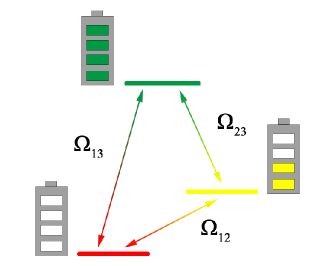
Figure 1: Visualisation of the concept of a closed-loop three-level quantum battery. Three discrete energy states represent different states of the battery and are charged through three laser fields: $\Omega_{12},\Omega_{23}$ and $\Omega_{13}$. The spaces in the battery show the degree of charge, and the spaces gradually fill up from bare to fully charged batteries. When the three-level system is in the ground state (red), it is equivalent to a bare battery. We regard the intermediate state (yellow) as a partially charged battery. It represents a fully charged battery at the maximum excited state (green).

Without loss of generality, we assume a nondegenerate quantum battery by a Hamiltonian Allahverdyan et al. (2004),

$$H_{0}=\sum_{n}^{d}\varepsilon_{n}\left|\varepsilon_{n}\right\rangle\left\langle\varepsilon_{n}\right|,\quad\varepsilon_{1}<\varepsilon_{2}<\cdots<\varepsilon_{d}.$$ (1)

Our major objective is to analyze the performance of three-level quantum battery, so that $d=3$. We sketch our proposal in Fig. 1. At the initial moment, the system is prepared in the ground state, representing a depleted battery. To drive the system and promote transitions between the energy levels, one utilizes auxiliary fields, i.e., suddenly switching on a transitional Hamiltonian $H_{1}$. We seek to inject as much energy into the quantum batteries as possible during the charging time $\tau$. The full Hamiltonian which describes the dynamics of the battery can be written as

$$H(t)=H_{0}+\lambda(t)H_{\mathrm{1}}(t),$$ (2)

where $\lambda(t)$ is a dimensionless parameter, whose explicit dependence on time $t$ manifests the external control exerted on the system. For the sake of definiteness, we assume $\lambda(t)$ equal to one for $0<t<\tau$ and zero elsewhere. The character of the Hamiltonian $H_{\mathrm{1}}(t)$ is equivalent to a quantum charger, and $\lambda(t)$ guarantees it charge the battery only at $t\in[0,\tau]$.

The transitional Hamiltonian $H_{1}$ reads Barfuss et al. (2018)

$$\begin{split}&H_{\mathrm{1}}(t)=\\ &\hbar\left[\begin{array}[]{ccc}{0}&{\Omega_{12}(t)e^{-i(\omega_{12}t+\phi_{1})}}&{\Omega_{13}(t)e^{-i(\omega_{13}t+\phi_{3})}}\\ {\Omega_{12}(t)e^{i(\omega_{12}t+\phi_{1})}}&{0}&{\Omega_{23}(t)e^{-i(\omega_{23}t+\phi_{2})}}\\ {\Omega_{13}(t)e^{i(\omega_{13}t+\phi_{3})}}&{\Omega_{23}(t)e^{i(\omega_{23}t+\phi_{2})}}&{0}\end{array}\right]\end{split}$$ (3)

Here $\hbar$ is the reduced Planck constant. $\Omega_{12},\Omega_{23}$ and $\Omega_{13}$ are amplitudes of three driving fields (see Fig. 1). $\omega_{12},\omega_{23},\omega_{13}$ and $\phi_{1},\phi_{2},\phi_{3}$ are frequencies and phases of three driving fields, respectively. We assume they are real and positive.

The Hamiltonian $H_{0}$ plays a crucial role in how much energy a quantum battery stores. The total energy in the battery at time $t$ is implicitly

$$E(t)=\operatorname{Tr}\left\{H_{0}\rho(t)\right\},$$ (4)

with $\rho=\sum_{n}r_{n}\left|r_{n}\right\rangle\left\langle r_{n}\right|$ being the density matrix of system Binder et al. (2015). And the time evolution of quantum state is according to the Liouville-von Neumann equation Alicki and Fannes (2013)

$$\dot{\rho}(t)=\frac{1}{i\hbar}\left[H(t),\rho(t)\right].$$ (5)

Indeed, we explore the dynamics of the system charging in a time-dependent interaction picture and the Hamiltonian $H(t)$ can be written as Kölbl et al. (2019)

$$H_{\mathrm{int}}(t)=\hbar\left[\begin{array}[]{ccc}{0}&{\Omega_{12}(t)}&{\Omega_{13}(t)e^{i\phi}}\\ {\Omega_{12}(t)}&{0}&{\Omega_{23}(t)}\\ {\Omega_{13}(t)e^{-i\phi}}&{\Omega_{23}(t)}&{0}\end{array}\right],$$ (6)

where we assumed that the driving fields are in resonance. The global driving-field phase $\phi=\phi_{1}+\phi_{2}-\phi_{3}$, which strongly influences the resulting dynamics Barfuss et al. (2018).

The time evolution of quantum state is obtained from the equation

$$\dot{\rho}_{\mathrm{int}}(t)=\frac{1}{i\hbar}\left[H_{\mathrm{int}}(t),\rho_{\mathrm{int}}(t)\right],$$ (7)

with $\rho_{\text{int }}(t)=e^{iH_{0}t}\rho(t)e^{-iH_{0}t}$. In our charging protocol, we already assumed that three external fields mentioned above are in resonance with the levels of the battery. Therefore, the population in each energy level satisfies

$$P_{n}=\operatorname{Tr}\left\{\hat{P}_{n}\rho_{\text{int }}(t)\right\}=\operatorname{Tr}\left\{\hat{P}_{n}\rho(t)\right\},$$ (8)

where $\hat{P}_{n}$ represents the projector $\hat{P}_{n}=\left|\varepsilon_{n}\right\rangle\left\langle\varepsilon_{n}\right|$. Furthermore, $\operatorname{Tr}\left\{H_{0}\rho_{\text{int }}(t)\right\}=\operatorname{Tr}\left\{H_{0}\rho(t)\right\}$, the extractable work can be obtained from the difference,

$$C(t)=\operatorname{Tr}\left\{H_{0}\rho_{\text{int }}(t)\right\}-\varepsilon_{1}.$$ (9)

Allowing the system to undergo adiabatic dynamics, the evolved state is $|\psi^{ad}(t)\rangle$, and the ergotropy is

$$C(t)= \langle\psi^{ad}(t)|H_{0}|\psi^{ad}(t)\rangle-\langle\varepsilon_{1}|H_{0}|\varepsilon_{1}\rangle$$

$$= \langle\psi^{ad}(t)|H_{0}|\psi^{ad}(t)\rangle-\varepsilon_{1}.$$ (10)

Notice that if $\varepsilon_{1}=0$ then ergotropy coincides with the mean energy of $\rho_{\text{int}}$, i.e., $C(t)=E(t)$. For the total charging time $\tau$, the corresponding work is $C(\tau)$

$$P(\tau)=\frac{C(\tau)}{\tau}.$$ (11)

In Ref. Santos et al. (2019b), $\Omega_{13}=0$, the STIRAP protocol can avoid the oscillatory behavior and achieve a stable charging process. Consistent with the previous works Santos et al. (2019b), we take

$$\Omega_{12}(t)=\Omega_{0}f(t),\quad\Omega_{23}(t)=\Omega_{0}[1-f(t)],$$ (12)

where $\Omega_{0}$ is a constant and $f(t)=t/\tau$. In what follows, we calculate and analyze the ergotropy and the charging power for different parameters shown in the interaction Hamiltonian $H_{\mathrm{int}}$.

III Dynamics in closed-loop quantum batteries

We now analyze the charging process focusing on the closed-loop quantum battery. We first consider a special case, i.e., the phase $\phi=\pi/2$. The corresponding eigenstates of the Hamiltonian (6) are

$$|E_{-}(t)\rangle = \frac{1}{\sqrt{2}}\left(\frac{\Omega_{12}(t)\Omega_{23}(t)}{\Omega(t)\Omega_{1}(t)}-i\frac{\Omega_{13}(t)}{\Omega_{1}(t)}\right)|\varepsilon_{1}\rangle$$ (13)

$$-\frac{1}{\sqrt{2}}\left(\frac{\Omega_{23}(t)}{\Omega_{1}(t)}-i\frac{\Omega_{12}(t)\Omega_{13}(t)}{\Omega(t)\Omega_{1}(t)}\right)|\varepsilon_{2}\rangle$$

$$+\frac{1}{\sqrt{2}}\frac{\Omega_{1}(t)}{\Omega(t)}|\varepsilon_{3}\rangle,$$

$$|E_{0}(t)\rangle = \frac{\Omega_{23}(t)}{\Omega(t)}|\varepsilon_{1}\rangle+i\frac{\Omega_{13}(t)}{\Omega(t)}|\varepsilon_{2}\rangle-\frac{\Omega_{12}(t)}{\Omega(t)}|\varepsilon_{3}\rangle,$$ (14)

$$|E_{+}(t)\rangle = \frac{1}{\sqrt{2}}\left(\frac{\Omega_{12}(t)\Omega_{23}(t)}{\Omega(t)\Omega_{1}(t)}+i\frac{\Omega_{13}(t)}{\Omega_{1}(t)}\right)|\varepsilon_{1}\rangle$$ (15)

$$+\frac{1}{\sqrt{2}}\left(\frac{\Omega_{23}(t)}{\Omega_{1}(t)}+i\frac{\Omega_{12}(t)\Omega_{13}(t)}{\Omega(t)\Omega_{1}(t)}\right)|\varepsilon_{2}\rangle$$

$$+\frac{1}{\sqrt{2}}\frac{\Omega_{1}(t)}{\Omega(t)}|\varepsilon_{3}\rangle,$$

with the eigenenergies $E_{0}(t)=0$ and $E_{\pm}(t)=\pm\hbar\Omega(t)$, where $\Omega^{2}(t)=\Omega^{2}_{12}(t)+\Omega^{2}_{23}(t)+\Omega^{2}_{13}(t)$ and $\Omega^{2}_{1}(t)=\Omega^{2}_{13}(t)+\Omega^{2}_{23}(t)$.

To achieve an efficient charged state, we employ the STIRAP technique Vitanov et al. (2017); Dou et al. (2013) and assume the initial state of system $|\psi(0)\rangle=|E_{0}(t)\rangle=|\varepsilon_{1}\rangle$. Therefore, the initial values of the control fields satisfy $\Omega_{12}(0)=\Omega_{13}(0)=0$ and $\Omega_{23}(t)\neq 0$. When the system undergoes adiabatic dynamics, the evolved state becomes $|\psi^{ad}(t)\rangle=|E_{0}(t)\rangle$. Then the ergotropy is

$$C(t)=\frac{\Omega^{2}_{23}}{\Omega^{2}(t)}\varepsilon_{1}+\frac{\Omega^{2}_{13}}{\Omega^{2}(t)}\varepsilon_{2}+\frac{\Omega^{2}_{12}}{\Omega^{2}(t)}\varepsilon_{3}-\varepsilon_{1}.$$ (16)

One find that the ergotropy depends on the final values for control fields $\Omega_{12}(t),\Omega_{23}(t)$ and $\Omega_{13}(t)$ at some cutoff time $\tau_{c}$ and can arrive the maximal value $C_{max}=\varepsilon_{3}-\varepsilon_{1}$ when $\Omega_{13}(\tau_{c})=\Omega_{23}(\tau_{c})=0$ and $\Omega_{12}(\tau_{c})\neq 0$. To the end we select the suitable control fields, such that the above boundary conditions are satisfied. In the following calculation we take $\varepsilon_{1}=0$, $\varepsilon_{2}=\hbar$, $\varepsilon_{3}=1.95\hbar$, respectively. The control fields $\Omega_{13}(t)$ is taken as

$$\Omega_{13}(t)= \Omega_{0}\sin(\pi t/\tau),\,\,\Omega_{0}(1-\cos(2\pi t/\tau)),$$ (17)

$$\Omega_{0}(1-\cos(2\pi t/\tau))^{2}.$$

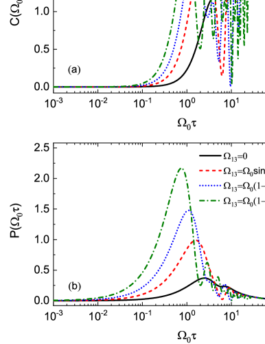
Figure 2: (a) The dependence of the ergotropy on $\Omega_{0}\tau$ for $\Omega_{13}=\Omega_{0}\sin(\pi t/\tau)$ (red dashed), $\Omega_{13}=\Omega_{0}(1-\cos{(2\pi t/\tau)})$ (blue dotted) and $\Omega_{13}=\Omega_{0}(1-\cos{(2\pi t/\tau)})^{2}$ (olive dash-dotted). The solid black curve represents the non-closed case $\Omega_{13}=0$. (b) The average charging power as a function of $\Omega_{0}\tau$. Color coding and labeling is the same as in (a). All shown data have been computed by setting $\phi=\pi/2$.

The dependence of the ergotropy $C(\tau)$ and the average charging power $P(\tau)$ on $\tau$ is indicated in Fig. 2 for several categories of $\Omega_{13}$. Here $\Omega_{0}\tau$ is the dimensionless parameter. In order to analyze the advantages of closed-loop, we also plot the situation of non-closed loop (solid black line), corresponding to $\Omega_{13}=0$. Different from the non-closed loop case, the evolution process of ergotropy is divided into four windows along the $\tau$ dimension. For a fast evolution, the ergotropy is almost $0$ due to being far from the adiabatic limit at these timescales. With increasing $\tau$ the ergotropy grows monotonically to a maximum value, which achieves a fully charged state (corresponding to the maximum charging energy), then begins to oscillate, and finally reaches and stays at it’s maximum value for large timescales. We also clearly see that, for different control fields, because of the different transfer time of all the population from the initial ground state to the maximally excited state, the minimal time to reach the maximum ergotropy for the first time is different. As a result, for fast protocol our batteries fail to charge (corresponding to small average power). However, as $\tau$ increases, the average charging power also increases until it reaches a maximum value at some point. Beyond this timescale, the average power will be less than this maximum value.

It is interesting to note that the maximum average charging power of closed-loop battery is greatly improved, even far beyond the ideal maximum power value of non-closed-loop three-level quantum battery, corresponding to the most powerful charging obtainable with minimum quantum speed limit time and the maximum charging energy Santos et al. (2019b). More detailed, the value is close to $4$ times of that for the original non-closed loop battery with $\Omega_{13}=\Omega_{0}\sin(\pi t/\tau)$. When we select the control field $\Omega_{13}=\Omega_{0}(1-\cos{(2\pi t/\tau)})^{n}$ ($n=1,2,\cdots$), the value will continue to increase and is close to $6$ times that for the original non-closed loop battery when $\Omega_{13}=\Omega_{0}(1-\cos{(2\pi t/\tau)})$ and more than $8$ times as high when $\Omega_{13}=\Omega_{0}(1-\cos{(2\pi t/\tau)})^{2}$. Further study shows that the maximum average charging power can be increased by increasing the index $n$ of control field. Furthermore, compared with the ergotropy of the non-closed loop system at its maximum average charging power, the closed-loop batteries charged by three laser fields can store more ergotropy, i.e., the existence of the control field $\Omega_{13}$ can greatly improve the maximum average charging power and the extractable energy, thus accelerating the charging process. Therefore, for an optimized $\Omega_{13}$, the system can realize high efficient and stable charging process as long as we immediately turn off the $H_{1}$ after the moment of reaching the maximum average charging power.

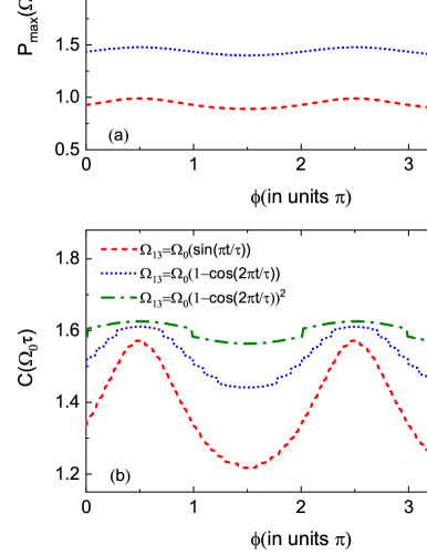
Figure 3: (a) The maximum charging power and (b) the corresponding energy as a function of $\phi$ for $\Omega_{13}(t)=\Omega_{0}\sin(\pi t/\tau)$ (red dashed), $\Omega_{13}(t)=\Omega_{0}(1-\cos{(2\pi t/\tau)})$ (blue dotted) and $\Omega_{13}=\Omega_{0}(1-\cos{(2\pi t/\tau)})^{2}$ (olive dash-dotted).

So far we only consider the case of the total driving phase $\phi=\pi/2$. To further demonstrate the effect of the phase on the charging process, we calculate the maximum average charging power and the charging energy at different phases. Fig. 3 shows the maximum average charging power and the corresponding energy as a function of $\phi$ under the different control field $\Omega_{13}$. No matter what the control field is, the maximum charging power and energy have the same period $2\pi$ and reach their maximum value at $\phi=\pi/2$. As the index $n$ increases, the maximum average charging power and the corresponding energy increase and the amplitude of oscillation decreases. For a clearer and more comprehensive understanding of the effect of phase on the charging energy and the average charging power, in Fig. 4, we display the charging energy and the average charging power as a function of both phase $\phi$ and charging time $\tau$ for different control field $\Omega_{13}$. The blue zones correspond to low value whereas red areas indicate high value. The plot reveals main features of the charging process with phase and charging time. It’s apparent that phase plays a non-negligible role in charging process. The charging energy and the maximum average charging power are obviously periodic with $2\pi$ and can obtain the maximum value at the position $\phi=\pi/2$.

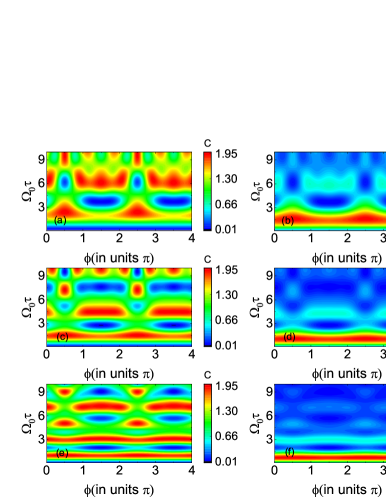
Figure 4: Contour plots of charging energy (left columns) and power (right columns) as the function of phase $\phi$ and charging time $\tau$ for different $\Omega_{13}$. (a) and (b) $\Omega_{13}=\Omega_{0}\sin(\pi t/\tau)$. (c) and (d) $\Omega_{13}=\Omega_{0}(1-\cos{(2\pi t/\tau)})$. (e) and (f) $\Omega_{13}=\Omega_{0}(1-\cos{(2\pi t/\tau)})^{2}$.

IV Quantum battery implement in nitrogen-vacancy spin

There are several physical systems to implement the closed-loop three-level quantum battery such as trapped ion systems or superconducting circuit systems. Here we briefly describe a scheme which coherently drives the NV spin using a combination of time-varying magnetic and strain fields to implement a three-level quantum battery. The negatively charged NV centre in the diamond lattice forms an $S=1$ spin system. Under an appropriate rotating frame and the resonant case, the dynamics of the NV spin are described by the Hamiltonian (6) Barfuss et al. (2018); Goldman et al. (2015). Conveniently, the initialization of the system can be realized by means of optical spin pumping under green laser excitation. Even at room temperatures, the spin of the NV can also be initialized easily. This character makes it become platforms for quantum information processing Ajisaka and Band (2016). The three eigenstates of the spin operater $\hat{S}_{z}$ are $|-1\rangle$, $|0\rangle$ and $|+1\rangle$, which correspond to $\left|\varepsilon_{1}\right\rangle$, $\left|\varepsilon_{2}\right\rangle$ and $\left|\varepsilon_{3}\right\rangle$ in our battery, respectively. Thus, one can prepare the system correspond to a bare quantum battery in $\left|\varepsilon_{1}\right\rangle$ at first, and then utilize a time-varying strain field to drive $|-1\rangle\leftrightarrow|+1\rangle$ transition and microwave magnetic fields to drive $|0\rangle\leftrightarrow|\pm 1\rangle$ transitions. The NV spin can be optically read out by virtue of its spin-dependent fluorescence. At last, the ergotropy and charging power of the three-level quantum battery can be obtained by uncomplicated calculation.

V Conclution

We have introduced the concept of a ”closed-loop three-level quantum battery”, which is a three-level system driven by three available transitions forming a closed-contour interaction. We show the performance of the quantum battery can be greatly improved by choosing an appropriate the third driving field. The closed-contour interaction makes the maximum average charging power can be greatly increased, even far beyond the most ideal maximum power value of non-closed-loop three-level quantum battery. In addition, the charging energy and power can reach the peak value at phase $\phi=\pi/2$ and vary with phase with a period of $2\pi$. Finally, we have briefly described the scheme of realizing closed-loop three-level quantum battery by a nitrogen-vacancy spin system.