AGN X-ray irradiation of CO gas in NGC 2110 revealed by Chandra and ALMA

Abstract

We report spatial distributions of the Fe-K$\alpha$ line at 6.4 keV and the CO($J$ = 2–1) line at 230.538 GHz in NGC 2110, which are respectively revealed by Chandra and ALMA at $\approx$ 0.5 arcsec. A Chandra 6.2–6.5 keV-to-3.0–6.0 keV image suggests that the Fe-K$\alpha$ emission extends preferentially in a northwest-to-southeast direction out to $\sim$ 3 arcsec, or 500 pc, on each side. Spatially-resolved spectral analyses support this by finding significant Fe-K$\alpha$ emission lines only in northwest and southeast regions. Moreover, their equivalent widths are found $\sim$ 1.5 keV, indicative for the fluorescence by nuclear X-ray irradiation as the physical origin. By contrast, CO($J$ = 2–1) emission is weak therein. For quantitative discussion, we derive ionization parameters by following an X-ray dominated region (XDR) model. We then find them high enough to interpret the weakness as the result of X-ray dissociation of CO and/or H₂. Another possibility also remains that CO molecules follow a super-thermal distribution, resulting in brighter emission in higher-$J$ lines. Further follow-up observations are encouraged to draw a conclusion on what predominantly changes the inter-stellar matter properties, and whether the X-ray irradiation eventually affects the surrounding star formation as an AGN feedback.

1 Introduction

Harsh radiation from a mass accreting super-massive black hole (SMBH), or an active galactic nucleus (AGN), can change thermal and chemical properties of the surrounding inter-stellar medium (ISM). The SMBH is usually present in the center of a massive galaxy, and it has been suggested that the SMBH and host galaxy have grown while affecting each other (i.e., the co-evolution; e.g., Magorrian et al., 1998; Marconi & Hunt, 2003; Gebhardt et al., 2000; Ferrarese & Merritt, 2000; Kormendy & Ho, 2013). This implies that the host galaxy has formed stars while being subject to the AGN radiation. Thus, towards the complete understanding of the galaxy growth, the study of the AGN radiative effect is important.

The AGN is more X-ray luminous than stars, and affects the ISM in a fundamentally different way. Also, because of the high energy of X-ray photons, the AGN X-ray emission is expected to largely affect ISM properties. Such a region subject to the X-ray emission is conventionally referred to as the X-ray dominated region (XDR; e.g., Krolik & Kallman, 1983; Lepp & Dalgarno, 1996; Maloney et al., 1996; Maloney, 1999), and has been often studied theoretically (Usero et al., 2004; Meijerink & Spaans, 2005; Meijerink et al., 2007; Proga et al., 2014). There was even a prediction that the X-ray emission changes the initial stellar mass function by evaporating a thinner part of a gas cloud and compressing its thicker part (Hocuk & Spaans, 2010, 2011). Among the predictions compared with observational works (e.g., García-Burillo et al., 2010; Izumi et al., 2015; Kawamuro et al., 2019), a noticeable point regarding the co-evolution would be the X-ray dissociation of molecular gas. Given a good correlation between the star-forming region and molecular gas distribution (e.g., Kennicutt et al., 2007; Bigiel et al., 2008) and theoretical arguments (e.g., Glover & Clark, 2012; Byrne et al., 2019), star formation can be active in regions where hydrogen molecules are efficiently produced. Thus, qualitatively, X-ray emission that dissociates molecular gas may work to inhibit star formation, or as a negative AGN feedback.

X-ray-irradiated regions have been often probed with Chandra (e.g., Young et al., 2001; Wang et al., 2009; Marinucci et al., 2012, 2013, 2017; Gómez-Guijarro et al., 2017; Fabbiano et al., 2017, 2019a, 2019b; Kawamuro et al., 2019) by exploiting its high angular resolution ($<$ 0.5 arcsec). A simple way to unveil such regions is to map the Fe-K$\alpha$ fluorescent line at 6.4 keV, originated by the ionization of a K-shell electron due to an X-ray above the 7.1 keV edge energy. In comparison with focusing on soft X-ray emission, adopted in many studies, we can probe X-ray-irradiated denser gas. This is because the hard X-ray emission that produces the Fe emission can penetrate into the gas deeply, and the Fe emission can break out of the gas due to the high penetrating power. Little contamination from stellar light above 7.1 keV (e.g., LaMassa et al., 2012; Kawamuro et al., 2013; LaMassa et al., 2017) is also an advantage to purely trace regions subject to AGN emission.

In this paper, we discuss ISM properties in the central $\approx$ 1.3 kpc of NGC 2110, which hosts an obscured AGN, based on the Fe-K$\alpha$ and CO($J$ = 2–1) emission lines. Recently, Rosario et al. (2019) found a region with weak CO($J$ = 2–1) emission within $\sim$ 600 pc of NGC 2110. This study was then followed by Fabbiano et al. (2019a), who reported the presence of soft X-ray photons in the region (see also Evans et al., 2006). Following them, we provide further pieces of information obtained by constraining the Fe-K$\alpha$ distribution, eventually enabling quantitative discussion for the weak CO($J$ = 2–1) emission.

This paper is organized as follows. In Section 2, we briefly describe what were previously found and suggested for NGC 2110. Then, Sections 3 and 4 present a summary of our Chandra and ALMA datasets and their analyses, respectively. Section 5 is dedicated to discussion. Finally, the summary of this paper is presented in Section 6. Unless otherwise noted, errors are quoted at the 1$\sigma$ confidence level for a single parameter of interest.

2 NGC 2110

NGC 2110 is located at a redshift of 0.00779 ($cz$ = 2335$\pm$20 km s^-1), determined from an optical Mg $b$ absorption line by Nelson & Whittle (1995). Under the assumption of a $\Lambda$CDM cosmology with $H_{0}$ = 70 km m^-1 Mpc^-1, $\Omega_{\rm m}=0.3$, and $\Omega_{\Lambda}=0.7$, the luminosity and angular distances are 33.6 Mpc and 33.0 Mpc (i.e., 1 arcsec $\approx$ 160 pc). An optical center of the galaxy is (R.A., Dec. = 88.047420, $-$7.456212 = 5h52m11.381s, $-$7d27m22.36s) (Clements, 1983). The galaxy is categorized as an early type S0 galaxy (de Vaucouleurs et al., 1991), and the stellar mass was estimated to be $\sim 10^{10.6}~{}M_{\rm sun}$ (Koss et al., 2011). Also, molecular and atomic hydrogen gases distribute on scales of $\sim$ 200–600 pc, and their masses would amount to $\sim 10^{8}~{}M_{\rm sun}$ and $\sim 10^{7}~{}M_{\rm sun}$, respectively (e.g., Gallimore et al., 1999; Rosario et al., 2019).

NGC 2110 hosts a type-2 AGN (Bradt et al., 1978; McClintock et al., 1979; Shuder, 1980). The detection of polarized broad H$\alpha$ emission by Moran et al. (2007) suggests the presence of a type-1-AGN-like core, however obscured by dust. Because of the obscuration, the nuclear structure was often investigated by X-ray observations since Bradt et al. (1978). Observed X-ray spectra showed Fe-K$\alpha$ emission with a velocity width of $\sim$ 2000 km s^-1 (Shu et al., 2010) and time-variable absorptions with column densities of $N_{\rm H}\sim{\rm a~{}few}\times 10^{22}$ cm^-2 (e.g., Bradt et al., 1978; Hayashi et al., 1996; Rivers et al., 2014; Marinucci et al., 2015; Kawamuro et al., 2016). Thus, an amount of matter is likely located around the nucleus, and may form a putative torus. Absorption-corrected 2–10 keV luminosities were measured to be $\sim 10^{42-43}$ erg s^-1(e.g., Mushotzky, 1982; Weaver et al., 1995; Rivers et al., 2014; Kawamuro et al., 2018).

NGC 2110 has been a good target to study impacts of the jet and nuclear radiation on the ISM simultaneously. Indeed, a radio jet in a north-south direction is clearly seen from parsec to $\approx$ 600 pc scales (e.g., Ulvestad & Wilson, 1983; Nagar et al., 1999; Mundell et al., 2000). For example, an impact of the jet on the ISM was indicated by NIR [Fe II] emission bright in the north-south direction (e.g., Storchi-Bergmann et al., 1999; Durré & Mould, 2014; Diniz et al., 2015, 2019). On the other hand, regions subject to the nuclear UV radiation were suggested from distributions of hydrogen emission lines extending with an angle $\sim 30$ degrees from north to west (e.g., Wilson & Baldwin, 1985; Pogge, 1989; Mulchaey et al., 1994; González Delgado et al., 2002; Ferruit et al., 2004). Moreover, soft X-ray ($<~{}2$ keV) emission found out to $\sim$ a few kpc would suggest that the nuclear X-ray emission also contributes to excitation of ambient gas (Weaver et al., 1995; Evans et al., 2006; Fabbiano et al., 2019a).

3 Observation data

3.1 Chandra data

We analyzed one Chandra/ACIS-S (Garmire et al. 2003) imaging data of NGC 2110 (ObsID = 883) to probe X-ray-irradiated regions. Our analysis utilized the standard data analysis package CIAO (ver. 4.9) and a calibration database of CALDB (ver. 4.7.6). The raw data was reprocessed with the standard chandra_repro command. Periods with slight increase of background rates were found during the observation and were filtered out. An exposure of $\approx$ 45 ksec was left for further analyses. The pile-up effect, where more than one photons are counted as one photon within a single readout, was checked by using pileup_map. Only in the central 1 arcsec region (Figure 1), pile-up fractions were larger than 5%. Because our interest is in spatially-extended emission, we do not further discuss the central region.

Accuracy of the absolute coordinates of the Chandra image was checked by comparing with the radio emission. The peak of counts at 3–7 keV, where a nuclear-emission was dominant (Section 4.1.2; e.g., Rivers et al., 2014; Kawamuro et al., 2016), was found at (R.A., Dec. = 5h52m11.367s, $-$7d27m22.496s). This differed only by $\approx$ 0.15 arcsec from the radio emission peak at (R.A, Dec. = 05h52m11.377s, $-$7d27m22.492s) (see Section 4.2.1). Thus, no correction for the image was made.

3.2 ALMA

We utilized the Band 6 ($\sim$ 270 GHz) ALMA data with the program ID = #2012.1.00474.S (PI: N. Nagar). The data was taken with an on-source exposure of 2.2 ksec on 2015 March 14, when 37 antennas were operated. It covered CO($J$ = 2–1) emission at the rest-frame frequency of $\nu_{\rm rest}$ = 230.538 GHz. The maximum angular scale, which can be recovered from observations, was $\sim$ 8.6 arcsec ($\approx$ 1.38 kpc) from a minimum projected baseline of 19 m. This was larger than the central $\approx$ 1.3 kpc, or 8 arcsec, scale structure of interest. A spectral window that covered CO($J$ = 2–1) emission had a total bandwidth of 1.875 GHz with a central frequency of 228.792 GHz and 1920 channels. The raw spectral resolution was 0.98 MHz ($\approx$ 1.3 km s^-1), but eight spectral elements were binned to achieve a resolution of $\approx$ 7.8 MHz (10 km s^-1), as explained in Section 4.2.1. Standard flux, bandpass, and phase calibrations were made by observing Ganymede, J0423-0120, and J0541-0541, respectively. Detailed analyses of this data is described in Section 4.2.

4 Data analysis

4.1 Chandra data analysis

In the former part of this subsection (Sections 4.1.1 and 4.1.2), we describe imaging analyses and show extended X-ray emission. Then, we present spatially-resolved spectral analyses, confirming the extension.

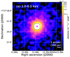
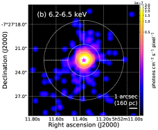
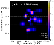
Figure 1: (a,b) X-ray images at 3.0–6.0 keV and 6.2–6.5 keV within the central $\approx$ 14$\times$14 arcsec² region. The size of each pixel is 0.0625$\times$0.0625 arcsec², and adaptive smoothing was performed with a Gaussian kernel with FWHM = 0.492 arcsec. In (a), the pixels with pile-up fractions larger than 5% are enclosed by the gray solid line. In (b), the inner annulus between 1 and 2 arcsec was used to estimate the nuclear X-ray emission (Section 4.1.2), and on the outside, the four fan-shaped regions between 2 and 5 arcsec with an angle of 90 degrees were defined to extract spectra of extended X-ray emission (Section 4.1.3). (c) Ratios between the 6.2–6.5 keV and 3.0–6.0 keV images from which un-resolved nuclear emission was subtracted. The size of the region is the same as those of (a) and (b). Original images before calculating the ratios had a pixel size of 0.49$\times$0.49 arcsec². Adaptive smoothing with a Gaussian kernel with FWHM = 1.0 arcsec was made after the calculation. Each of the figures has a magenta or white star at the 3–7 keV peak.

4.1.1 Observed high-angular resolution X-ray images

We show Chandra 3.0–6.0 keV and 6.2–-6.5 keV images in Figure 1, respectively giving brief impressions about spatial distributions of continuum emission and the 6.4 keV Fe-K$\alpha$ line. They were made by sampling counts on a sub-pixel scale of 0.0615$\times$0.0615 arcsec², that is, by adopting the energy-dependent sub-pixel event-re-positioning algorithm (e.g., Tsunemi et al., 2001; Mori et al., 2001; Li et al., 2003, 2004). Then, we made smoothing via a Gaussian kernel with FWHM = 0.492 arcsec, corresponding to the ACIS CCD pixel size. Exposure maps for the softer and harder X-ray images were calculated at intermediate energies of 4.5 keV and 6.35 keV, respectively. At first glance, we can see 6.2–6.5 keV emission elongated in a northwest-southeast direction (Figure 1(b)). Such can be seen also in the 3.0–6.0 keV image (Figure 1(a)).

4.1.2 Spatial distribution of Fe-K$\alpha$ emission

We revealed extended Fe-K$\alpha$ emission by removing unresolved nuclear emission, which spreads by a point spread function. The nuclear image was created by simulating observations where the nuclear emission only existed. Our simulations were made using a Monte-Carlo simulator of the MARX software (ver. 5.3.3; Davis et al. 2012), which generates photons and projects them onto a detector plane while taking account of the mirror and detector responses.

We determined the input nuclear emission spectrum by extracting its component from a spectrum in an annulus between 1 and 2 arcsec (Figure 1(b)). Therein, the pile-up effect was negligible. A background spectrum was estimated from a blank 50 arcsec radius circle located in the same CCD. The 0.5–7.0 keV spectrum was fitted with absorbed and un-absorbed power-law components, two Gaussian functions (zgauss in XSPEC terminology) for the 1.74 keV Si-K$\alpha$ and 6.4 keV Fe-K$\alpha$ lines, and an optically-thin thermal component (i.e., the apec model in XSPEC). By considering poor photon statistics, the photon indices of the power-law components were fixed to 1.65, a canonical value suggested from past studies of NGC 2110 (e.g., Evans et al., 2007; Kawamuro et al., 2016). Also, because of the CCD poor energy resolution, we fixed the line widths at 0.1 eV. Adopting a width smaller than those constrained by Chandra grating observations (i.e., $\approx$ 2300 km s^-1; Shu et al., 2010) did not affect our result. The best-fit model was determined based on the $C$-statistic (Cash, 1979), appropriate even for low photon statistics. Goodness of fit was examined by following the procedure given in Kaastra (2017). The expected $C$-statistic value ($C_{\rm exp}$) and variance ($C_{\rm var}$) from a model was compared with an observed value ($C_{\rm obs}$). A model would be acceptable at the 90% confidence level if $C_{\rm obs}<C_{\rm exp}+1.28\times\sqrt{C_{\rm var}}$ (Kaastra, 2017). Eventually, we obtained the best-fit model with $C_{\rm obs}$/$C_{\rm exp}$/$C_{\rm var}$ = 356/472/29. A good agreement between the data and best-fit model is found in Figure 2. The resultant parameters are summarized in Table 1. An observed flux at 2–10 keV, where the absorbed power-law component is dominant, is $2.3\times 10^{-11}$ erg cm^-2 s^-1, and the intrinsic luminosity of the absorbed power-law component at 2–10 keV was $4\times 10^{42}$ erg s^-1, which is within those measured previously (e.g., Marinucci et al., 2015). The equivalent width of the Fe-K$\alpha$ line was 152${}^{+141}_{-107}$ eV, consistent with those previously measured for NGC 2110 by Marinucci et al. (2015) as well as those typical in moderately obscured AGNs (e.g., 30–500 eV; Kawamuro et al., 2016).

Figure 2: X-ray spectrum (black crosses) extracted from an annulus between 1 and 2 arcsec and the best-fit model (black solid line). An absorbed power-law component (blue dashed line), 1.74 keV Si-K$\alpha$ line (blue dotted line), and 6.4 keV Fe-K$\alpha$ one (blue dot-dashed line) were assumed to come from the unresolved central X-ray source. Additionally, an un-absorbed power-law (black dot-dashed line) and the optically-thin thermal emission (apec; black dashed line) were fitted to mainly reproduce soft X-ray emission. The lower data represent the residuals.

Table 1: Best-fit parameters of the annulus spectrum

	Parameter	Best-fit	Units
(1)	$N_{\rm H}$	$4.0^{+0.7}_{-0.6}$	1022 cm-2
(2)	$\Gamma$	1.65
(3)	$N^{\rm abs}_{\rm PL}$	$6.3^{+0.6}_{-0.5}$	10-3 photons keV-1 cm-2 s-1
(4)	$N^{\rm un-abs}_{\rm PL}$	$0.51\pm 0.14$	10-3 photons keV-1 cm-2 s-1
(5)	$kT$	$0.57^{+0.18}_{-0.23}$	keV
(6)	$N_{\rm apec}$	$1.8^{+0.09}_{-0.08}$	$10^{-4}$
(7)	$N_{\rm Fe-K{\alpha}}$	$46^{+26}_{-22}$	10-6 photons cm-2 s-1
(8)	$N_{\rm Si-K{\alpha}}$	$69^{+19}_{-18}$	10-6 photons cm2 s-1
(9)	$F_{\rm 2-10~{}keV}$	2.3	10-11 erg cm-2 s-1
(10)	$L_{\rm 2-10~{}keV,PL}$	3.7	1042 erg s-1
(11)	$C_{\rm obs}$/$C_{\rm exp}$/$C_{\rm var}$	356/472/29

Note. — Rows: (1) Hydrogen column density in the sightline. (2) Photon index of the absorbed and un-absorbed power-law components. The value was fixed. (3,4) Normalizations of the two power-law components at 1 keV. (5,6) Temperature and normalization of the apec model (see https://heasarc.gsfc.nasa.gov/xanadu/xspec/manual/node134.html for more details). (7,8) Normalizations of the Gaussian models (zgauss) for the Fe-K$\alpha$ and Si-K$\alpha$ emission. (9) Observed flux at 2–10 keV, where the absorbed power-law component is dominant. (10) Intrinsic luminosity of the absorbed power-law component at 2–10 keV. (11) $C$-statistic values.

From the best-fit spectral components, we defined the sum of the absorbed power-law and two emission lines as the nuclear emission. The other components (i.e., the un-absorbed power-law emission and the thermal emission) would largely include in-situ emission given that they were un-absorbed. Indeed, if a component is from the nucleus, it should be absorbed by the sightline obscuration.

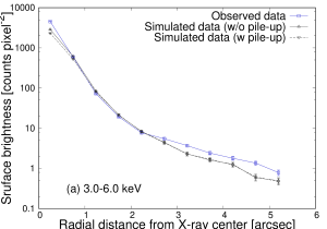
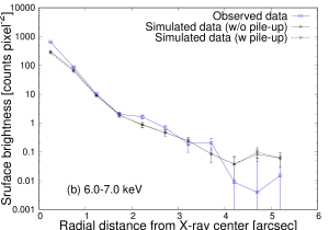
Figure 3: (a) Comparison between observed (blue) and simulated (black) radial profiles of the surface brightness in units of counts pixel^-2 at 3.0–6.0 keV. The black solid and dashed lines show those without and with the pile-up effect, respectively. (b) Same as (a), but for the 6.0–7.0 keV band.

With the defined spectrum, we simulated Chandra imaging observations. The source position was set to the 3–7 keV peak (magenta stars in Figure 1). The other parameters necessary for the simulation were set so as to reproduce the ObsID = 883 observation. To mitigate uncertainty of each Monte-Carlo simulation result, we created 1000 images, and took their average.

The validity of our simulation was examined by comparing the radial profiles of the observed and simulated images. Figure 3 shows broad consistency between the profiles, or the images. Although a factor of $\sim$ 2 difference was seen in the innermost pixels, this would be due to incompleteness of the simulation software as was remarked by the developers. Because the simulated profile did not exceed the observed one significantly at any radii and energies, we concluded to proceed with the above simulation results.

At last, in Figure 1(c) we show the ratios between 6.2–6.5 keV and 3.0–6.0 keV images from which the nuclear emission was subtracted. The ratio is a proxy of the equivalent width (EW) of the Fe-K$\alpha$ line. The X-ray photons were sampled at a larger pixel size of 0.49$\times$0.49 arcsec² to increase S/N ratios. Particularly in the 3.0–6.0 keV image, we excluded pixels with counts smaller than 2, corresponding to $\approx$ 1$\sigma$ level for the mean value of 0 counts (Gehrels, 1986). This was made to avoid extreme ratios due to quite low photons in the 3.0–6.0 keV image. Exposure maps were created in the same way as for the previous images. The image of the ratios was smoothed with the Gaussian kernel with FWHM = 1.0 arcsec. We can see a structure extending preferentially in a northwest-southeast direction out to $\approx$ 3 arcsec, or $\sim$ 500 pc, on each side. We caution that the ratio image changes depending on the significance criterion imposed on the 3.0–6.0 keV image. However, the extended morphology can be seen generally in most cases. Also, we emphasize that the result is consistent with the model-independent image of Figure 1(b) and is confirmed by the spectral analysis below.

4.1.3 Spatially resolved X-ray spectral analysis

We confirmed the un-isotropic extended Fe-K$\alpha$ emission suggested from Figure 1 by spatially-resolved spectral analysis. We focused on four fan-like sub-regions, outlined in Figure 1(b). They were referred to as NW, SW, SE, and NE, depending on their directions from the nucleus. Starting from north, the fan-like regions were defined to have an angle of 90 degrees. Their inner and outer radii were 2 arcsec and 5 arcsec, respectively. A background spectrum was estimated from a blank 50 arcsec radius circle located in the same CCD. The spectra were binned so as to have at least one count at each bin. Two different types of response files for the in-situ emission and the nuclear emission were generated using the CIAO tool specextract.

While taking account of the nuclear emission (the sum of the blue lines in Figure 2) as a fixed component, we fitted the spectra with a power-law and a Gaussian function, reproducing continuum emission and the Fe-K$\alpha$ line, respectively. The line width was fixed at 0.1 eV. Therefore, the normalization and photon index of the power-law component and the normalization of the Gaussian function were left as free parameters. The spectra folded by the response functions and their best-fit models are shown in Figure 4. The parameters are summarized in Table 2.

Table 2: Best-fit parameters of the four sub-regions spectra with the power-law and Gaussian models

		NE	NW	SE	SW
(1)	$\Gamma$	$-1.3^{+1.4}_{-1.6}$	$1.0^{+0.9}_{-0.8}$	$1.2^{+1.0}_{-0.9}$	$-4.1^{+1.9}_{-3.3}$
(2)	$N_{\rm PL}$	$0.12^{+0.96}$	$7.0^{+15.4}_{-4.9}$	$8.0^{+21.4}_{-5.9}$	$0.0010^{+0.0253}$	10-6 photons keV-1 cm-2 s-1
(3)	$N_{\rm Fe-K{\alpha}}$	$0.12^{+4.86}$	$16^{+7}_{-6}$	$15^{+7}_{-6}$	$0.96^{+5.28}$	10-7 photons cm-2 s-1
(4)	EWFe-Kα	—	1.5${}^{+2.1}_{-1.0}$	1.6${}^{+2.6}_{-1.1}$	—	keV
(5)	$C_{\rm obs}$/$C_{\rm exp}$/$C_{\rm var}$	126/160/14	105/154/14	104/143/13	101/161/15

Note. — Rows: (1,2) Photon index and normalization at 1 keV of the power-law component. (3) Normalization of the Gaussian model (zgauss), reproducing the Fe-K$\alpha$ emission. (4) Equivalent width of the Fe-K$\alpha$ emission. (5) $C$-statistic values.

An important point is the significant detection of the Fe-K$\alpha$ emission lines only in the NW and SE regions. The difference in $C_{\rm obs}$ between the models with and without the line was found $\sim$ 12 in the NW and SE cases, suggesting the high significance. This was not the case in the NE and SW regions. The ratio between the sum of the NW and SE extended components and the unresolved nuclear one was estimated to be $\sim$ 7%. The EWs in the NW and SE regions were found 1.5–1.6 keV. One might be confused by the EWs, because such high EWs were observed often in Compton-thick AGNs (Ricci et al., 2015; Tanimoto et al., 2018) but NGC 2110 hosts just a lightly obscured AGN with $N_{\rm H}\sim 10^{22}$ cm^-2 (Marinucci et al., 2015). As later detailed in Section 5.1, the high EWs can be because we just see only reflected emission without transmitted emission. In this case, such high EWs can be reproduced with various column densities (e.g., see the right panel of Figure 14 of Ikeda et al., 2009). This is natural given that we focus solely on the extended components. Instead, the observed EW from the much brighter nuclear component ($\approx 150$ eV in Section 4.1.2 and Figure 2) is better to be compared with those generally obtained, or those from spatially un-resolved spectra. In the case, that is consistent with those of moderately obscured AGNs with $N_{\rm H}=10^{22-24}$ cm^-2 (e.g., 30–500 eV; Kawamuro et al., 2016).

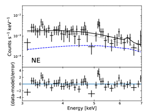
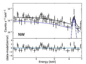
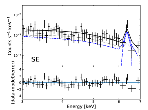
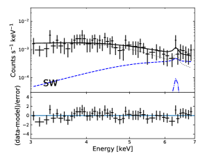
Figure 4: X-ray spectra (black crosses) extracted from the four fan-like regions defined in Figure 1(b). The best-fit models (solid line) were determined by fitting the contaminating X-ray emission from the nuclear point source (dotted gray line) and the extended emission of interest (blue dashed line), consisting of a power-law and Fe-K$\alpha$ emission (blue dot-dashed line). The lower data represent the residuals.

We further fitted a reflection model of the Ikeda torus model (Ikeda et al., 2009) to the spectra in the NW and SE regions, where the Fe-K$\alpha$ emission was significantly detected. By this analysis, it was possible to roughly estimate a column density along the propagating path of the nuclear X-ray emission. The torus model calculated spectra from a spherical structure with a bi-conical gas-free region irradiated by a central point source with a power-law spectrum. The photon index of the power-law spectrum was fixed to 1.65 (e.g., Evans et al., 2007; Kawamuro et al., 2016). The half opening angle and our inclination angle from the polar axis were by default set to 60 degrees and 30 degrees. Different choices of the parameters did not affect our conclusion. Free parameters left were the normalization of the power-law component and the column density in the equatorial plane. By adopting the $C$-statistic method, we got acceptable fits (i.e., $C_{\rm obs}<C_{\rm exp}+1.28\times\sqrt{C_{\rm var}}$) for both the NW and SE spectra. The obtained parameters are summarized in Table 3. The column densities were found $\sim 10^{23}$ cm^-2 at most.

Table 3: Best-fit parameters of the two sub-regions spectra with the torus models

		NW	SE
(1)	$\Gamma$	1.65	1.65
(2)	$N_{\rm PL}$	$1.5^{+5.0}_{-0.8}$	$1.9^{+4.3}_{-1.2}$	10-3 photons keV-1 cm-2 s-1
(3)	$N^{\rm eq}_{\rm H}$	$4.6^{+6.8}$	$3.0^{+7.2}$	1022 cm-2
(4)	EWFe-Kα	1.6	1.9	keV
(5)	$C_{\rm obs}$/$C_{\rm exp}$/$C_{\rm var}$	105/154/14	105/143/13

Note. — Rows: (1,2) Photon index and normalization at 1 keV of the power-law component. The photon index was fixed. (3) Hydrogen column density in the equatorial plane. (4) Equivalent width of the Fe-K$\alpha$ line. (5) $C$-statistic values.

4.2 ALMA data analysis

In the following two subsections, first we show basic pieces of information on the CO($J$ = 2–1) line, and then we present its geometrical and kinematic properties.

4.2.1 Basic properties of CO($J$ = 2–1) emitting gas

The ALMA data was reduced via the Common Astronomy Software Applications (CASA) (McMullin et al., 2007) with ver. 4.2.2, the same as in the Quality Verification by the ALMA Regional Center, and then was analyzed via the CASA with ver. 5.1.1. To extract the data of CO($J$ = 2–1) emission, continuum level was determined by fitting line-free channels with the 1st-ordered function, and was subtracted from the data cube via the task uvcontsub. The product was then deconvolved by the clean task with the Briggs-weighting with robust = 0.5 and gain = 0.1. The achieved synthesized beam was $0.52\times 0.83$ arcsec² with P.A. = $-75.17$ degrees. The channels were binned so that the velocity resolution was $\approx$ 10 km s^-1. The primary beam image correction was made via impbcor. The final continuum-subtracted data had a RMS noise of 0.76 mJy beam^-1. This was estimated from the CO emission-free channels. The moment 0, 1, and 2 maps of the CO($J$ = 2–1) line were made, and are shown in Figure 5. The zeroth moment was calculated over the $V_{\rm LSR}$ range of 1900–2800 km s^-1. The other moment maps were calculated with 5$\sigma$ clipping in the same $V_{\rm LSR}$ range. Continuum emission was also mapped by the clean task (Figure 6). The achieved synthesized beam was $0.49\times 0.81$ arcsec² with P.A. = $-73.80$ degrees. The center of the nuclear component was estimated to be (R.A., Dec. = 5h52m11.377s, $-$7d27m22.492s) by fitting a single Gaussian function through the imfit task.

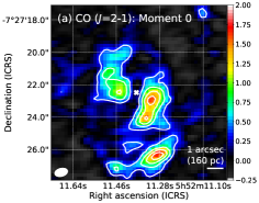
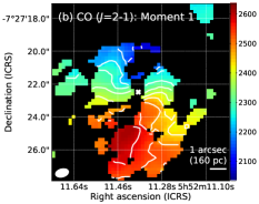
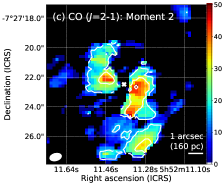
Figure 5: (a) Moment 0 map of the CO($J$ = 2–1) line in units of Jy beam^-1 km s^-1. This was created in the range $V_{\rm LSR}$ = 1900–2800 km s^-1. The contour levels are 5$\sigma$, 10$\sigma$, 15$\sigma$, and 20$\sigma$, where $\sigma$ is 0.073 Jy beam^-1 km s^-1. (b) Moment 1 map in units of km s^-1, where the contours represent the $V_{\rm LSR}$ with steps of 50 km s^-1 from 2086 km s^-1. (c) Moment 2 map in units of km s^-1 with the contours separated by 10 km s^-1. The beam size (bottom-left filled ellipse) is 0.52$\times$0.83 arcsec² with PA = $-$75.17 degrees. In all figures, the region is the central $\approx$11$\times$11 arcsec², and the white cross is located at the center of the continuum emission (R.A., Dec. = 5h52m11.377s, $-$7d27m22.492s).

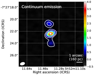
Figure 6: Continuum intensity map in units of mJy beam^-1 with contours of 5$\sigma$, 15$\sigma$, and 45$\sigma$, and 135$\sigma$, where $\sigma$ is 0.030 mJy beam^-1. The beam size (bottom-left filled ellipse) is 0.49$\times$0.81 arcsec² with PA = $-$73.80 degrees. The white cross is located at the center of the continuum emission (R.A., Dec. = 5h52m11.377s, $-$7d27m22.492s).

4.2.2 Geometrical structure and kinetic properties of CO gas

We revealed a three-dimensional structure of the CO($J$ = 2–1) emitting gas disk to finally estimate a molecular gas volume density, essential to discuss the ionization state of the molecular gas. We reconstructed the structure by fitting a model of concentric tilted rings to the observed velocity field. Then, the rotation velocity and velocity dispersion were available from the model. With these, we derived the scale heights, or the thicknesses of the rings. Combined with an observed gas surface density, those eventually permitted an estimate of the molecular gas volume density, used to calculate ionization parameters in Section 5.2.

A fit of the concentric titled rings to the observed CO($J$ = 2–1) data was made by adopting the 3D Barolo code (Di Teodoro & Fraternali, 2015). This code takes account of beam-smearing of an intrinsic structure. The main seven parameters are the dynamical center, systemic velocity ($V_{\rm sys}$), thickness of the ring, rotation velocity ($V_{\rm rot}$), velocity dispersion ($\sigma_{\rm dis}$), angle between the polar axis and our sightline ($i$), and P.A. ($\phi$), which can be determined in each of the rings. The P.A. is defined as an angle from north to the major axis of the receding half component in the anti-clockwise direction. The first three parameters were fixed. The dynamical center was set to the radio continuum one, as determined in Section 4.2.1. The systematic velocity was set to 2335 km s^-1. The thickness of each ring was fixed at 0.5 arcsec ($\approx$ 80 pc) to be consistent with scale heights derived from the resultant rotation velocity and velocity dispersion. We then fitted the remaining four parameters by starting from initial guesses. We set $i=$ 65 degrees as the initial guess in all the rings. A similar value was adopted by Ramakrishnan et al. (2019), who also studied a kinematic structure of CO($J$ = 2–1) in NGC 2110. The adopted angle is larger than $i=$ 53 degrees, which was inferred from an observed aspect ratio between the major and minor axes of a H$\alpha$+[N II] emission distribution (e.g., Wilson & Baldwin, 1985) and was sometimes adopted in past studies (e.g., Gallimore et al., 1999). It is however not necessary to follow it, given that the H$\alpha$+[N II] distribution may be disturbed by the nuclear emission. Also, if the thickness of the morphology cannot be ignored, a larger angle is more plausible. Finally, our choice ($i$ = 65 degrees) was made because we obtained a rotation curve that monotonously increased with radius, whereas we were not able to obtain such a curve with the smaller one ($i$ = 53 degrees). However, we note that even if we adopt $i$ = 53 degrees, we can get a result that does not affect our conclusion, or the estimates of the scale heights. The other three parameters were adjusted so that $V_{\rm rot}$ and $\sigma_{\rm dis}$ continuously changed across the rings. We determined the free parameters every 0.25 arcsec from the starting point at 0.75 arcsec, given the beam size of $0.52\times 0.83$ arcsec². The innermost part ($\leq 0.5$ arcsec) was not considered because of the weak CO($J$ = 2–1) emission. Our fit took account of channels in the velocity range 1900 km s^-1–2800 km s^-1 with significance larger than 5$\sigma$ (= 3.8 mJy beam^-1).

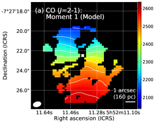
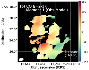
Figure 7: (a) Model moment 1 map of the CO($J$ = 2–1) emission, where the contours represent the $V_{\rm LSR}$ with steps of 50 km s^-1 from 2086 km s^-1. (b) Difference between the observed and modeled moment 1 maps.

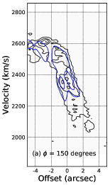
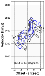
Figure 8: (a) Position-velocity diagrams along position angle of 150 degrees. The model is indicated by the blue contours, while the observed data by the black ones. The contour levels are 1$\sigma$, 3$\sigma$, 5$\sigma$, and 7$\sigma$, where $\sigma$ is 0.76 mJy beam^-1. A significant ($\sim 7\sigma$) non-rotating motion with 2600 km s^-1, or with an excess velocity of 100 km s^-1, is seen around $-3$ arcsec. (b) Same as (a), but for the position angle of 60 degrees.

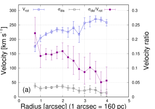
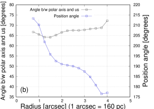
Figure 9: (a) Rotation velocity, velocity dispersion, and their ratio as a function of radius from the radio continuum center. (b) Angle between the polar axis and our sightline and position angle as a function of radius from the radio continuum center.

The Momonet 1 map of our ring model and residuals against the observed one are seen in Figure 7(a) and (b), respectively. Generally, we can see good agreement, except for a southeast red component, as is also seen at $\approx$ 7$\sigma$ in a position velocity diagram of Figure 8(a). Note that the diagrams in Figure 8 were created by averaging pixels in slits with 2.5 arcsec width perpendicular to directions of $\phi=150$ degrees and $\phi=60$ degrees. The former angle was selected to show the significance of the red component, while the latter was adopted to just show the perpendicular diagram. Interpretation of the red component in excess of $\sim$ 100 km s^-1 is ambiguous; this may be a high-velocity inflow deviating from an outer rotating disk, or may be an outflow driven by the nuclear radiation. Note that the jet is less likely to be associated with the flow, given its south-north axis (Figure 6). The flux density integrated between 2590–2640 km s^-1 in a 1.5 arcsec circular region was 1.3 Jy km s^-1. By adopting Equation (1) in Rosario et al. (2019), the molecular gas mass was estimated to be $\sim 10^{6}~{}M_{\rm sun}$. Given the physical extension of $\sim 3$ arcsec, or 500 pc, the characteristic flow rate was calculated to be $\sim$ 0.2 $M_{\rm sun}$ yr^-1. Note that the equation we considered was the same as for a thin shell-like geometry (i.e., Equation (4) of Maiolino et al. 2012).

The parameters given by our model are seen as a function of radius from the radio continuum center in Figure 9. The ratios between the rotation velocity and velocity dispersion were $\approx$ 0.05–0.15 in the range 160–640 pc. Therefore, the thicknesses, $\approx 2\times$ the scale heights, were estimated to be within $\sim$ 50–110 pc. This range is consistent with the assumed thicknesses (i.e., 80 pc) of the rings.

5 Discussion

Our discussion is made along with Figure 10, which shows a detailed geometrical structure of the CO($J$ = 2–1) emission and our schematic pictures within the central $\approx$ 1.3 kpc of NGC 2110.

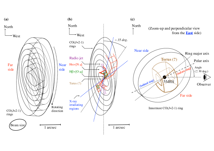
Figure 10: (a) Geometrical configuration of the CO($J$ = 2–1) rings in the central $\approx$ 1.3 kpc of NGC 2110. The innermost and outermost rings correspond to those with radii of 0.75 arcsec and 3.75 arcsec, respectively. (b) Spatial comparison between the radio jet (solid purple lines; Ulvestad & Wilson, 1983; Gallimore et al., 1999), the H$\alpha$+[N II] (red shaded regions) and H$\beta$+[O III] (green shaded regions) emission (Rosario et al., 2010), the X-ray irradiating regions (blue dashed lines), and CO($J$ = 2–1) rings (black solid lines). Regarding the H$\alpha$+[N II] emission, darker red indicates brighter emission. An obscuring torus, speculated from the morphologies of the ionized regions, is also indicated in the center. For clarity, the thicknesses of the CO rings are omitted. (c) Speculated innermost region seen from the East direction.

5.1 Extended Fe-K$\alpha$ emitting region and nuclear obscuration

Based on Figure 1(b) and (c), we have suggested that the Fe-K$\alpha$ emission is spatially collimated and extends in a northwest-southeast direction out to $\sim$ 3 arcsec ($\sim$ 500 pc) on each side (Figure 1). This was also indicated by the spatially-resolved spectral analysis (Figure 4).

To discuss the physical origin, the EW of the Fe-K$\alpha$ emission is useful. As listed in Table 3, those in the northwest and southeast regions are as high as $\approx$ 1.5 keV. We caution that they do not include the un-resolved nuclear emission and are derived from the extended components. Such high EWs can be explained by X-ray irradiation of ambient gas. In the case, a direct photo-ionizing X-ray source is not seen in the sightline and only the reflected X-ray emission is seen, thus favoring a high EW ($\sim$ 1 keV; e.g., Nobukawa et al., 2010). It would be fine to rule out another idea that the Fe-K$\alpha$ emission is the result of the scattering of the nuclear emission. This is because the emission line should be accompanied by stronger continuum emission as is seen in un-obscured AGNs ($\sim 200$ eV; Ricci et al., 2014a, b), favoring a lower EW. Also, the collisional ionization would be unlikely as the primary process because a lower EW is expected due to strong bremsstrahlung emission under the line (e.g., Nobukawa et al., 2010).

The nuclear emission likely plays a major role in the irradiative process, compared with emission from the jet. Although the beamed X-ray emission from the jet may be more energetic (e.g., Weaver et al., 1995) and its un-isotropic emission can naturally reproduce a collimated structure, its contribution would be rather minor. The north-south axis of the jet (Ulvestad & Wilson, 1983; Nagar et al., 1999) is different from that seen for the Fe-K$\alpha$ emission (Figure 10).

Given that the nuclear X-ray emission is more or less isotropic (e.g., Liu et al., 2014), a collimating structure is needed to be consistent with the observed morphology. A putative AGN torus is a plausible one (e.g., Urry & Padovani, 1995). Its presence was inferred from past optical and NIR observations (e.g., Rosario et al., 2010; Diniz et al., 2015, 2019). Rosario et al. (2010) showed that optical emission from ionized atoms (i.e., H$\alpha$+[N II] and H$\beta$+[O III]) extends preferentially in a northwest-southeast direction with P.A. $\sim$ $-$35 degrees (Figure 10(b)). Similar morphologies can be seen at NIR hydrogen emission lines (e.g., Br$\gamma$ and Pa$\beta$; Diniz et al., 2015, 2019). Thus, as depicted in Figure 10(b), we suggest that the nuclear X-ray emission is also collimated by the same torus structure as the emission lines in the optical and NIR bands. Note that the X-ray emission may widely irradiate the ambient gas than the longer wavelength emission given the higher penetrating power.

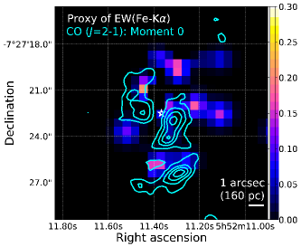
Figure 11: Ratio between the 6.2–6.5 keV and 3.0–6.0 keV images (color), a proxy of the Fe-K$\alpha$ line EW, and the CO($J$ = 2–1) velocity-integrated intensity map (cyan), drawn at the same levels in Figure 5(a). The white star is located at the 3–7 keV peak.

5.2 Spatial distributions of Fe-K$\alpha$ and CO($J$ = 2–1) emission and XDR model

The Fe-K$\alpha$ emission is spatially compared with the CO($J$ = 2–1) emission in Figure 11. Their spatial anti-correlation is seen; the CO emission is stronger in the northeast and southwest islands, whereas the Fe-K$\alpha$ emission is bright in the northwest and southeast directions (see Section 5.1).

We quantitatively discuss the physical origin of the anti-correlation, while referring to an XDR model (Maloney et al., 1996). The model considered gas illuminated by power-law X-ray emission. The key parameter, which determines fractional abundances of atomic and molecular gas species (see their Figure 3), is the effective ionization parameter, calculated as

$$\xi_{\rm eff}\simeq 0.1\frac{L_{44}}{n_{4}R^{2}_{100}N^{\alpha}_{{\rm H},22}},$$ (1)

where $L_{44}$, $n_{4}$, $R_{100}$, $N_{\rm H,22}$, and $\alpha$ represents the 1–100 keV luminosity in units of $10^{44}$ erg s^-1, the hydrogen molecular gas density in units of $10^{4}$ cm^-3, the distance the X-ray source in units of 100 pc, the column density of the gas in units of $10^{22}$ cm^-2 that attenuates the incident X-ray flux, and an X-ray photon index dependent value, respectively. The last factor ($\alpha$) is specifically expressed as $\alpha=$ ($\Gamma$+2/3)/(8/3), taking account of the fact that softer spectra are more heavily extincted.

Un-absorbed 2–10 keV luminosity was estimated in various epochs, and varied within 0.4–3.5$\times 10^{43}$ erg s^-1(Marinucci et al., 2015). That corresponds to a 1–100 keV luminosity range 2–15$\times 10^{43}$ erg s^-1, where a photon index of 1.65 is assumed. Note that this index corresponds to $\alpha\approx$ 0.87. The density of the molecular hydrogen gas is estimated to be 120–270 cm^-3 by adopting a hydrogen molecular gas surface density of 650 $M_{\odot}$ pc^-2 in the central region with faint CO($J$ = 2–1) emission between the east and west CO islands (Rosario et al., 2019) and the disk thickness ($\approx$ 50–110 pc). The distance $R_{100}$ is 4.8, corresponding to 3 arcsec. Given that distance and the density range, $N_{\rm H}$ $\sim~{}3\times 10^{23}$ cm^-2 are expected, where we assume the uniform gas density distribution. This is close to the upper bound of those from the spectral fittings in Section 4.1.3 (i.e., $N_{\rm H}<10^{23}$ cm^-2). As a result, the ionization parameters in NW and SE are conservatively calculated to be $\log\xi_{\rm eff}>-2.4$.

Based on the XDR model by Maloney et al. (1996), we can suggest some mechanisms, which suppress CO($J$ = 2–1) emission at the above-estimated ionization parameters. (1) The abundance of CO molecules is decreased due to dissociation by the charge exchange with He ions produced by the direct X-ray ionization. Such dissociation takes place also by Far-UV photons produced as the result of collision between photo-electrons and hydrogen species. (2) Hydrogen molecules are destroyed due to X-ray-produced photo-electrons. Given lower rotational-excitation efficiency of CO by H than by H₂ (Green & Thaddeus, 1976), that would also contribute to the weakness. (3) if achieved, a super-thermal CO population due to additional X-ray heating may also make a contribution. Note that one might consider a low line opacity of CO($J$ = 2–1) as the cause of the weakness. This can be achieved if $J$ = 2 level is populated by few CO molecules, but would be unlikely because $J$ = 2 level can be populated by many CO molecules in energetic circum-nuclear regions due to the low energy gap between $J$ = 2 and $J$ = 1. In summary, via the above three ways, the X-ray emission can weaken the CO($J$ = 2–1) emission.

To conclude what mechanism is at work, observing other lines is desired. For example, a [C I] line observation will be useful to examine the CO dissociation scenario by constraining the [C I]/CO line ratio. To discuss the H₂ dissociation, we need to estimate the amount of H₂ by a non-CO based method. One way is to utilize rotational quadrupole transition of H₂ (Togi & Smith, 2016). High sensitive spatially-resolved MIR spectroscopy by JWST/MIRI will be powerful for the estimate. The last super-thermal scenario will be investigated by observing CO at higher $J$ levels.

We note a discrepancy between an XDR prediction and a suggestion by Rosario et al. (2019), who also studied molecular gas in NGC 2110. The XDR model predicts dissociation of an amount of hydrogen molecules into atoms in the NW and SE regions. By contrast, based on Spitzer/IRS spectroscopy data, Rosario et al. (2019) suggested the presence of H₂ gas with a surface density ($>$ 180 $M_{\rm sun}$ pc^-2) comparable to that in the surrounding CO bright regions ($\sim$ 200-350 $M_{\rm sun}$ pc^-2), disfavoring the dissociation. Further discussion would need JWST/MIRI, if we follow the measurement method of Rosario et al. (2019). Briefly, they first determined a power-law temperature distribution consistent with observed H₂ populations at different excitation levels. They then derived the surface density while taking account of H₂ populations down to 50 K. This derivation is sensitive to the intensity at the lowest permitted rotational (quadrupole) transition of H₂ 0–0 S(0). However, only an upper-limit was obtained for the transition. Thus, its exact intensity constrained by MIRI is desired for further discussion.

5.3 Geometrical structures inferred from comparison between CO($J$ = 2–1) emission and optical one

We note our serendipitous finding in Figure 10 that the distribution of the H$\alpha$+[N II] emission, drawn based on Figure 3 in Rosario et al. (2010), looks like following some of the CO($J$ = 2–1) tilted rings obtained in Section 4.2.2. This may be a natural consequence of the irradiation by the nuclear source. Given the canonical definition of the ionization parameter (i.e., $\propto L/nR^{2}$, where $L$, $n$, and $R$ are the luminosity, density, and distance, respectively), an ionized region can extend up to a distance under a uniform gas distribution, consistent with the observed. Such was already argued in the past (e.g., Diniz et al., 2015). However, we emphasize that our constraint on the three-dimensional structure of the CO gas makes that picture clearer.

Also, we remark that from the configuration of the CO gas and ionized gas, it is possible to estimate an angle between our sightline and the polar axis of the ionization cone, or that of the torus. Rosario et al. (2010) suggested that the southern [O III] emission fainter than the northern one was due to dust extinction. Under the assumption that the dust distributes similarly to the molecular gas, it is suggested that the southern (the northern) polar axis of the ionization cone is preferentially located behind (before) the southern (northern) gas rings (Figure 10(c)). To accomplish such a configuration, the angle is required to be $\lesssim~{}30$ degrees. The AGN torus may have a half-opening angle of $\approx~{}37$ degrees, as estimated from its Eddington ratio ($\log\lambda_{\rm Edd}\sim-2$; Kawamuro et al., 2016) and a correlation between the Eddington ratio and the half-opening angle (Ricci et al., 2017). These results suggest that we see the nucleus almost at an intermediate angle between the obscuring torus and a region with less obscuration. Because of this angle, we may have often observed column-density variability and various obscuring components in the X-ray band (Rivers et al., 2014).

6 Summary

We have analyzed high-angular resolution ($\sim$ 0.5 arcsec) Chandra and ALMA data of an obscured AGN host of NGC 2110 to investigate AGN X-ray irradiation effects on the surrounding ISM. Our findings are summarized as follows.

• An $\sim$ 7% of the Fe-K$\alpha$ emission was spatially resolved by Chandra and extends preferentially in a northwest-to-southeast direction out to $\sim$ 3 arcsec (Figure 1(c) and Section 5.1). The EWs of the Fe-K$\alpha$ emission in the NW and SE regions were $\sim$ 1.5 keV (Figure 4 and Table 2), high enough to indicate X-ray irradiation as the physical origin.

• The tentative spatial anti-correlation between the Fe-K$\alpha$ and CO($J$ = 2–1) emission was found (Figure 11).

• The anti-correlation was discussed based on the ionization parameter defined in the XDR model (Section 5.2). The derived parameters predict some mechanisms at work that weaken the CO($J$ = 2–1) emission. The CO and/or H₂ molecules may be dissociated due to X-ray emission. Also, CO molecules may be super-thermalized by X-ray emission, making the low rotation level $J$ = 2–1 line weak. Follow-up observations of other lines (e.g., [C I], H₂ 0-0 S(0), and higher-$J$ CO lines) will be helpful for further discussion. As a final goal, such studies would lead to discussion on whether the X-ray irradiation eventually affects the surrounding star formation as an AGN feedback.

• Based on the geometrical structures of the molecular gas disk and the ionized regions, it was inferred that the polar axis of the ionization field, or the torus, is inclined by an angle $\lesssim 30$ degrees (Section 5.3 and Figure 10(c)).

In the future, sub-arcsec resolution observatories with larger effective areas (i.e., AXIS and Lynx; Reynolds & Mushotzky 2017 and Gaskin et al. 2018) will be launched. In such an era, they will enable us to more clearly map the Fe-K$\alpha$ line distribution of NGC 2110. Also, it will be possible to discuss XDRs in distant, more luminous AGNs, which have potential to more largely affect the surrounding ISM.

References

- Bigiel et al. (2008) Bigiel, F., Leroy, A., Walter, F., et al. 2008, AJ, 136, 2846, doi: 10.1088/0004-6256/136/6/2846
- Bradt et al. (1978) Bradt, H. V., Burke, B. F., Canizares, C. R., et al. 1978, ApJ, 226, L111, doi: 10.1086/182843
- Byrne et al. (2019) Byrne, L., Christensen, C., Tsekitsidis, M., Brooks, A., & Quinn, T. 2019, ApJ, 871, 213, doi: 10.3847/1538-4357/aaf9aa
- Canizares et al. (2005) Canizares, C. R., Davis, J. E., Dewey, D., et al. 2005, PASP, 117, 1144, doi: 10.1086/432898
- Cash (1979) Cash, W. 1979, ApJ, 228, 939, doi: 10.1086/156922
- Clements (1983) Clements, E. D. 1983, MNRAS, 204, 811, doi: 10.1093/mnras/204.3.811
- Davis et al. (2012) Davis, J. E., Bautz, M. W., Dewey, D., et al. 2012, in Society of Photo-Optical Instrumentation Engineers (SPIE) Conference Series, Vol. 8443, Proc. SPIE, 84431A
- de Vaucouleurs et al. (1991) de Vaucouleurs, G., de Vaucouleurs, A., Corwin, Herold G., J., et al. 1991, Third Reference Catalogue of Bright Galaxies
- Di Teodoro & Fraternali (2015) Di Teodoro, E. M., & Fraternali, F. 2015, MNRAS, 451, 3021, doi: 10.1093/mnras/stv1213
- Diniz et al. (2019) Diniz, M. R., Riffel, R. A., Storchi-Bergmann, T., & Riffel, R. 2019, MNRAS, 487, 3958, doi: 10.1093/mnras/stz1329
- Diniz et al. (2015) Diniz, M. R., Riffel, R. A., Storchi-Bergmann, T., & Winge, C. 2015, MNRAS, 453, 1727, doi: 10.1093/mnras/stv1694
- Durré & Mould (2014) Durré, M., & Mould, J. 2014, ApJ, 784, 79, doi: 10.1088/0004-637X/784/1/79
- Evans et al. (2006) Evans, D. A., Lee, J. C., Kamenetska, M., et al. 2006, ApJ, 653, 1121, doi: 10.1086/508680
- Evans et al. (2007) Evans, D. A., Lee, J. C., Turner, T. J., Weaver, K. A., & Marshall, H. L. 2007, ApJ, 671, 1345, doi: 10.1086/523037
- Fabbiano et al. (2017) Fabbiano, G., Elvis, M., Paggi, A., et al. 2017, ApJ, 842, L4, doi: 10.3847/2041-8213/aa7551
- Fabbiano et al. (2019a) Fabbiano, G., Paggi, A., & Elvis, M. 2019a, ApJ, 876, L18, doi: 10.3847/2041-8213/ab1c63
- Fabbiano et al. (2019b) Fabbiano, G., Siemiginowska, A., Paggi, A., et al. 2019b, ApJ, 870, 69, doi: 10.3847/1538-4357/aaf0a4
- Ferrarese & Merritt (2000) Ferrarese, L., & Merritt, D. 2000, ApJ, 539, L9, doi: 10.1086/312838
- Ferruit et al. (2004) Ferruit, P., Mundell, C. G., Nagar, N. M., et al. 2004, MNRAS, 352, 1180, doi: 10.1111/j.1365-2966.2004.08009.x
- Gallimore et al. (1999) Gallimore, J. F., Baum, S. A., O’Dea, C. P., Pedlar, A., & Brinks, E. 1999, ApJ, 524, 684, doi: 10.1086/307853
- García-Burillo et al. (2010) García-Burillo, S., Usero, A., Fuente, A., et al. 2010, A&A, 519, A2, doi: 10.1051/0004-6361/201014539
- Garmire et al. (2003) Garmire, G. P., Bautz, M. W., Ford, P. G., Nousek, J. A., & Ricker, George R., J. 2003, in Society of Photo-Optical Instrumentation Engineers (SPIE) Conference Series, Vol. 4851, Proc. SPIE, ed. J. E. Truemper & H. D. Tananbaum, 28–44
- Gaskin et al. (2018) Gaskin, J. A., Dominguez, A., Gelmis, K., et al. 2018, in Society of Photo-Optical Instrumentation Engineers (SPIE) Conference Series, Vol. 10699, Proc. SPIE, 106990N
- Gebhardt et al. (2000) Gebhardt, K., Bender, R., Bower, G., et al. 2000, ApJ, 539, L13, doi: 10.1086/312840
- Gehrels (1986) Gehrels, N. 1986, ApJ, 303, 336, doi: 10.1086/164079
- Glover & Clark (2012) Glover, S. C. O., & Clark, P. C. 2012, MNRAS, 421, 9, doi: 10.1111/j.1365-2966.2011.19648.x
- Gómez-Guijarro et al. (2017) Gómez-Guijarro, C., González-Martín, O., Ramos Almeida, C., Rodríguez-Espinosa, J. M., & Gallego, J. 2017, MNRAS, 469, 2720, doi: 10.1093/mnras/stx1037
- González Delgado et al. (2002) González Delgado, R. M., Arribas, S., Pérez, E., & Heckman, T. 2002, ApJ, 579, 188, doi: 10.1086/342675
- Green & Thaddeus (1976) Green, S., & Thaddeus, P. 1976, ApJ, 205, 766, doi: 10.1086/154333
- Hayashi et al. (1996) Hayashi, I., Koyama, K., Awaki, H., & Yamauchi, S. U. S. 1996, PASJ, 48, 219, doi: 10.1093/pasj/48.2.219
- Hocuk & Spaans (2010) Hocuk, S., & Spaans, M. 2010, A&A, 522, A24, doi: 10.1051/0004-6361/201015055
- Hocuk & Spaans (2011) —. 2011, A&A, 536, A41, doi: 10.1051/0004-6361/201117431
- Ikeda et al. (2009) Ikeda, S., Awaki, H., & Terashima, Y. 2009, ApJ, 692, 608, doi: 10.1088/0004-637X/692/1/608
- Izumi et al. (2015) Izumi, T., Kohno, K., Aalto, S., et al. 2015, ApJ, 811, 39, doi: 10.1088/0004-637X/811/1/39
- Kaastra (2017) Kaastra, J. S. 2017, A&A, 605, A51, doi: 10.1051/0004-6361/201629319
- Kawamuro et al. (2019) Kawamuro, T., Izumi, T., & Imanishi, M. 2019, PASJ, 71, 68, doi: 10.1093/pasj/psz045
- Kawamuro et al. (2016) Kawamuro, T., Ueda, Y., Tazaki, F., Ricci, C., & Terashima, Y. 2016, ApJS, 225, 14, doi: 10.3847/0067-0049/225/1/14
- Kawamuro et al. (2013) Kawamuro, T., Ueda, Y., Tazaki, F., & Terashima, Y. 2013, ApJ, 770, 157, doi: 10.1088/0004-637X/770/2/157
- Kawamuro et al. (2018) Kawamuro, T., Ueda, Y., Shidatsu, M., et al. 2018, ApJS, 238, 32, doi: 10.3847/1538-4365/aad1ef
- Kennicutt et al. (2007) Kennicutt, Robert C., J., Calzetti, D., Walter, F., et al. 2007, ApJ, 671, 333, doi: 10.1086/522300
- Kormendy & Ho (2013) Kormendy, J., & Ho, L. C. 2013, ARA&A, 51, 511, doi: 10.1146/annurev-astro-082708-101811
- Koss et al. (2011) Koss, M., Mushotzky, R., Veilleux, S., et al. 2011, ApJ, 739, 57, doi: 10.1088/0004-637X/739/2/57
- Krolik & Kallman (1983) Krolik, J. H., & Kallman, T. R. 1983, ApJ, 267, 610, doi: 10.1086/160897
- LaMassa et al. (2012) LaMassa, S. M., Heckman, T. M., & Ptak, A. 2012, ApJ, 758, 82, doi: 10.1088/0004-637X/758/2/82
- LaMassa et al. (2017) LaMassa, S. M., Yaqoob, T., Levenson, N. A., et al. 2017, ApJ, 835, 91, doi: 10.3847/1538-4357/835/1/91
- Lepp & Dalgarno (1996) Lepp, S., & Dalgarno, A. 1996, A&A, 306, L21
- Li et al. (2003) Li, J., Kastner, J. H., Prigozhin, G. Y., & Schulz, N. S. 2003, ApJ, 590, 586, doi: 10.1086/374967
- Li et al. (2004) Li, J., Kastner, J. H., Prigozhin, G. Y., et al. 2004, ApJ, 610, 1204, doi: 10.1086/421866
- Liu et al. (2014) Liu, T., Wang, J.-X., Yang, H., Zhu, F.-F., & Zhou, Y.-Y. 2014, ApJ, 783, 106, doi: 10.1088/0004-637X/783/2/106
- Magorrian et al. (1998) Magorrian, J., Tremaine, S., Richstone, D., et al. 1998, AJ, 115, 2285, doi: 10.1086/300353
- Maiolino et al. (2012) Maiolino, R., Gallerani, S., Neri, R., et al. 2012, MNRAS, 425, L66, doi: 10.1111/j.1745-3933.2012.01303.x
- Maloney (1999) Maloney, P. R. 1999, Ap&SS, 266, 207. https://arxiv.org/abs/astro-ph/9903275
- Maloney et al. (1996) Maloney, P. R., Hollenbach, D. J., & Tielens, A. G. G. M. 1996, ApJ, 466, 561, doi: 10.1086/177532
- Marconi & Hunt (2003) Marconi, A., & Hunt, L. K. 2003, ApJ, 589, L21, doi: 10.1086/375804
- Marinucci et al. (2017) Marinucci, A., Bianchi, S., Fabbiano, G., et al. 2017, MNRAS, 470, 4039, doi: 10.1093/mnras/stx1551
- Marinucci et al. (2013) Marinucci, A., Miniutti, G., Bianchi, S., Matt, G., & Risaliti, G. 2013, MNRAS, 436, 2500, doi: 10.1093/mnras/stt1759
- Marinucci et al. (2012) Marinucci, A., Risaliti, G., Wang, J., et al. 2012, MNRAS, 423, L6, doi: 10.1111/j.1745-3933.2012.01232.x
- Marinucci et al. (2015) Marinucci, A., Matt, G., Bianchi, S., et al. 2015, MNRAS, 447, 160, doi: 10.1093/mnras/stu2439
- McClintock et al. (1979) McClintock, J. E., van Paradijs, J., Remillard, R. A., et al. 1979, ApJ, 233, 809, doi: 10.1086/157444
- McMullin et al. (2007) McMullin, J. P., Waters, B., Schiebel, D., Young, W., & Golap, K. 2007, Astronomical Society of the Pacific Conference Series, Vol. 376, CASA Architecture and Applications, ed. R. A. Shaw, F. Hill, & D. J. Bell, 127
- Meijerink & Spaans (2005) Meijerink, R., & Spaans, M. 2005, A&A, 436, 397, doi: 10.1051/0004-6361:20042398
- Meijerink et al. (2007) Meijerink, R., Spaans, M., & Israel, F. P. 2007, A&A, 461, 793, doi: 10.1051/0004-6361:20066130
- Moran et al. (2007) Moran, E. C., Barth, A. J., Eracleous, M., & Kay, L. E. 2007, ApJ, 668, L31, doi: 10.1086/522697
- Mori et al. (2001) Mori, K., Tsunemi, H., Miyata, E., et al. 2001, in Astronomical Society of the Pacific Conference Series, Vol. 251, New Century of X-ray Astronomy, ed. H. Inoue & H. Kunieda, 576
- Mulchaey et al. (1994) Mulchaey, J. S., Wilson, A. S., Bower, G. A., et al. 1994, ApJ, 433, 625, doi: 10.1086/174671
- Mundell et al. (2000) Mundell, C. G., Wilson, A. S., Ulvestad, J. S., & Roy, A. L. 2000, ApJ, 529, 816, doi: 10.1086/308318
- Mushotzky (1982) Mushotzky, R. F. 1982, ApJ, 256, 92, doi: 10.1086/159886
- Nagar et al. (1999) Nagar, N. M., Wilson, A. S., Mulchaey, J. S., & Gallimore, J. F. 1999, ApJS, 120, 209, doi: 10.1086/313183
- Nelson & Whittle (1995) Nelson, C. H., & Whittle, M. 1995, ApJS, 99, 67, doi: 10.1086/192179
- Nobukawa et al. (2010) Nobukawa, M., Koyama, K., Tsuru, T. G., Ryu, S. G., & Tatischeff, V. 2010, PASJ, 62, 423, doi: 10.1093/pasj/62.2.423
- Pogge (1989) Pogge, R. W. 1989, ApJ, 345, 730, doi: 10.1086/167945
- Proga et al. (2014) Proga, D., Jiang, Y.-F., Davis, S. W., Stone, J. M., & Smith, D. 2014, ApJ, 780, 51, doi: 10.1088/0004-637X/780/1/51
- Ramakrishnan et al. (2019) Ramakrishnan, V., Nagar, N. M., Finlez, C., et al. 2019, MNRAS, 487, 444, doi: 10.1093/mnras/stz1244
- Reynolds & Mushotzky (2017) Reynolds, C. S., & Mushotzky, R. 2017, in AAS/High Energy Astrophysics Division #16, AAS/High Energy Astrophysics Division, 103.23
- Ricci et al. (2014a) Ricci, C., Ueda, Y., Ichikawa, K., et al. 2014a, A&A, 567, A142, doi: 10.1051/0004-6361/201322701
- Ricci et al. (2015) Ricci, C., Ueda, Y., Koss, M. J., et al. 2015, ApJ, 815, L13, doi: 10.1088/2041-8205/815/1/L13
- Ricci et al. (2014b) Ricci, C., Ueda, Y., Paltani, S., et al. 2014b, MNRAS, 441, 3622, doi: 10.1093/mnras/stu735
- Ricci et al. (2017) Ricci, C., Trakhtenbrot, B., Koss, M. J., et al. 2017, Nature, 549, 488, doi: 10.1038/nature23906
- Rivers et al. (2014) Rivers, E., Markowitz, A., Rothschild, R., et al. 2014, ApJ, 786, 126, doi: 10.1088/0004-637X/786/2/126
- Rosario et al. (2019) Rosario, D. J., Togi, A., Burtscher, L., et al. 2019, ApJ, 875, L8, doi: 10.3847/2041-8213/ab1262
- Rosario et al. (2010) Rosario, D. J., Whittle, M., Nelson, C. H., & Wilson, A. S. 2010, MNRAS, 408, 565, doi: 10.1111/j.1365-2966.2010.17153.x
- Shu et al. (2010) Shu, X. W., Yaqoob, T., & Wang, J. X. 2010, ApJS, 187, 581, doi: 10.1088/0067-0049/187/2/581
- Shuder (1980) Shuder, J. M. 1980, ApJ, 240, 32, doi: 10.1086/158204
- Storchi-Bergmann et al. (1999) Storchi-Bergmann, T., Winge, C., Ward, M. J., & Wilson, A. S. 1999, MNRAS, 304, 35, doi: 10.1046/j.1365-8711.1999.02360.x
- Tanimoto et al. (2018) Tanimoto, A., Ueda, Y., Kawamuro, T., et al. 2018, ApJ, 853, 146, doi: 10.3847/1538-4357/aaa47c
- Togi & Smith (2016) Togi, A., & Smith, J. D. T. 2016, ApJ, 830, 18, doi: 10.3847/0004-637X/830/1/18
- Tsunemi et al. (2001) Tsunemi, H., Mori, K., Miyata, E., et al. 2001, ApJ, 554, 496, doi: 10.1086/321338
- Ulvestad & Wilson (1983) Ulvestad, J. S., & Wilson, A. S. 1983, ApJ, 264, L7, doi: 10.1086/183935
- Urry & Padovani (1995) Urry, C. M., & Padovani, P. 1995, PASP, 107, 803, doi: 10.1086/133630
- Usero et al. (2004) Usero, A., García-Burillo, S., Fuente, A., Martín-Pintado, J., & Rodríguez-Fernández, N. J. 2004, A&A, 419, 897, doi: 10.1051/0004-6361:20035774
- Wang et al. (2009) Wang, J., Fabbiano, G., Elvis, M., et al. 2009, ApJ, 694, 718, doi: 10.1088/0004-637X/694/2/718
- Weaver et al. (1995) Weaver, K. A., Mushotzky, R. F., Serlemitsos, P. J., et al. 1995, ApJ, 442, 597, doi: 10.1086/175463
- Wilson & Baldwin (1985) Wilson, A. S., & Baldwin, J. A. 1985, ApJ, 289, 124, doi: 10.1086/162870
- Young et al. (2001) Young, A. J., Wilson, A. S., & Shopbell, P. L. 2001, ApJ, 556, 6, doi: 10.1086/321561