A non-cooperative meta-modeling game for automated third-party calibrating, validating, and falsifying constitutive laws with parallelized adversarial attacks
Abstract
The evaluation of constitutive models, especially for high-risk and high-regret engineering applications, requires efficient and rigorous third-party calibration, validation and falsification. While there are numerous efforts to develop paradigms and standard procedures to validate models, difficulties may arise due to the sequential, manual and often biased nature of the commonly adopted calibration and validation processes, thus slowing down data collections, hampering the progress towards discovering new physics, increasing expenses and possibly leading to misinterpretations of the credibility and application ranges of proposed models. This work attempts to introduce concepts from game theory and machine learning techniques to overcome many of these existing difficulties. We introduce an automated meta-modeling game where two competing AI agents systematically generate experimental data to calibrate a given constitutive model and to explore its weakness, in order to improve experiment design and model robustness through competition. The two agents automatically search for the Nash equilibrium of the meta-modeling game in an adversarial reinforcement learning framework without human intervention. In particular, a protagonist agent seeks to find the more effective ways to generate data for model calibrations, while an adversary agent tries to find the most devastating test scenarios that expose the weaknesses of the constitutive model calibrated by the protagonist. By capturing all possible design options of the laboratory experiments into a single decision tree, we recast the design of experiments as a game of combinatorial moves that can be resolved through deep reinforcement learning by the two competing players. Our adversarial framework emulates idealized scientific collaborations and competitions among researchers to achieve better understanding of the application range of the learned material laws and prevent misinterpretations caused by conventional AI-based third-party validation. Numerical examples are given to demonstrate the wide applicability of the proposed meta-modeling game with adversarial attacks on both human-crafted constitutive models and machine learning models.
1 Introduction and background
As constitutive models that predict material responses become increasingly sophisticated and complex, the demands and difficulties for accurately calibrating and validating those constitutive laws also increase (Dafalias, 1984; Thacker et al., 2004; Borja, 2013; Liu et al., 2016; De Bellis et al., 2017; Bryant and Sun, 2018; Na et al., 2019a, b). Engineering applications, particularly those involve high-risk and high-regret decision-makings, require models to maintain robustness and accuracy in unforeseen scenarios using as little amount of necessary calibration data as possible. Quantifying the reliability of a new constitutive law, however, is nontrivial. As many constitutive models are calibrated against limited amount and types of experimental data, identifying the reliable application range of these constitutive laws beyond the loading paths used in the calibration could be challenging. While an apparent good match between predictions and calibration data can be easily achieved by increasing the dimensionality of the parametric space of a given model, over-fitting may also jeopardize the application of the learned models in the case where the predicted loading path bears little resemblance to the calibration data (Wang et al., 2016; Gupta et al., 2019; Heider et al., 2020). Using such constitutive models therefore bears more risks for a third-party user who is unaware of the sensitivity of material parameters on the stress predictions. Furthermore, the culture and the ecosystem of the scientific communities often place a more significant focus on reporting the success of the material models on limited cases. Yet, precise and thorough investigations on the weakness and shortcomings of material models are important and often necessary, but they are less reported or documented in the literature due to the lack of incentive (Pack et al., 2014; Boyce et al., 2016).
Model calibration issues are critical not only for hand-crafted models but for many machine learning models and data-driven framework that either directly use experimental data to replace constitutive laws Kirchdoerfer and Ortiz (2016, 2017); He and Chen (2019) or generate optimal response surfaces via optimization problems (Bessa et al., 2017; Yang and Perdikaris, 2019; Zhu et al., 2019). The recent trend of using black-box deep neural network (DNN) to generate constitutive laws has made the reliability analysis even more crucial. At present, due to the lack of interpretability of predictions generated by neural network, reliability of DNN generated constitutive laws is often assessed through uncertainty quantification (UQ) (Yang and Perdikaris, 2019; Zhu et al., 2019). UQ can be conducted via different procedures, including Bayesian statistics, polynomial chaos expansion and Monte Carlo sampling where one seeks to understand how probability distributions of the input material parameters affect the outcomes of predictions, as often represented by some stress measures or performance metrics for solid mechanics applications. While UQ is a crucial step to ensure the readiness of constitutive laws for engineering applications, a common challenge is to detect rare events where a catastrophic loss of the prediction accuracy may occur in otherwise highly accurate constitutive laws.
The machine learning research community has been proposing methods to improve the interpolation and generalization capabilities, hence improving the predictive capability with exogenous data as well as reducing the epistemic uncertainties of trained neural network models. For instance, the active learning approaches (e.g. (Settles, 2009)), which is sometimes also referred as ”optimal experimental design” (Olsson, 2009), introduce query strategies to choose what data to be generated to reduce generalization errors, balance exploration and exploitation and quantify uncertainties. These approaches have repeatedly outperformed traditional ”passive learning” methods which involve randomly gathering a large amount of training data. Active learning is widely investigated using different deep learning algorithms like CNNs and LSTMS (Sener and Savarese, 2017; Shen et al., 2017). There is also research on implementing Generative Adversarial Networks (GANs) into the active learning framework (Zhu and Bento, 2017). With the increasing interest in deep reinforcement learning, researchers are trying to re-frame active learning as a reinforcement learning problem (Fang et al., 2017). Another recent study focuses on the ”semi-supervised learning” approaches (Zhu, 2005; Verma et al., 2019; Berthelot et al., 2019), which take advantage of the structures of unlabeled input data to enhance the ”interpolation consistency”, in addition to labeled training data. These recently developed techniques have shown some degrees of successes for image recognition, natural language processing, and therefore could potentially be helpful for mechanics problems.
The calibration, validation and falsification of material models have issues similar to those discussed above. Moreover, experimental data are often expensive to get in both time and cost. Hence, experimentalists would like to generate the least amount of data that can calibrate a constitutive model with the highest reliability and can also identify its limitations. Traditionally the decisions on which experiments to conduct are based on the human knowledge and experiences. We make an effort here to use AI to assist the decision-makings of experimentalists, which will be the first of its kind specifically targeting the automated design of data generation that can efficiently calibrate and falsify a constitutive model.
The major contribution of this paper is the introduction of a non-cooperative game that leads to new optimized experimental designs that both improves the accuracy and robustness of the predictions on unseen data, while at the same time exposing any potential weakness and shortcoming of a constitutive law.
We create a non-cooperative game in which a pair of agents are trained to emulate a form of artificial intelligence capable of improving their performance through trial and errors. The two agents play against each other in a turn-based strategy game, according to their own agendas and purposes respectively that serve to achieve opposite objectives. This setup constitutes a zero-sum game in which each agent is rewarded by competing against the opponent. While the protagonist agent learns to validate models by designing the experiments than enhance the model predictions, the adversary agent learns how to undermine the protagonist agent by designing experiments that expose the weakness of the models. The optimal game strategies for both players are explored by searching for Nash equilibrium (Nash et al., 1950) of the games using deep reinforcement learning (DRL).
With recent rapid development, DRL techniques have found unprecedented success in the last decades on achieving superhuman intelligence and performance in playing increasingly complex games: Atari (Mnih et al., 2013), board games (Silver et al., 2017b, a), Starcraft (Vinyals et al., 2019). AlphaZero (Silver et al., 2017b) is also capable of learning the game strategies of our game without human knowledge. By emulating the learning process of human learners through trial-and-error and competition, the DRL process enables both AI agents to learn from their own successes and failures but also through their competitions to master the tasks of calibrating and falsifying a constitutive law. The knowledge gained from the competitions will help us understanding the relative rewards of different experimental setup for validation and falsification mathematically represented by the decision trees corresponding to the protagonist and adversary agents.
The rest of the paper is organized as follows. We first describe the meta-modeling non-cooperative game, including the method to recast the design of experiments into decision trees (Section 2). Following this, we will introduce the detailed design of the calibration-falsification game for modeling the competition between the AI experimental agent and the AI adversarial agent (Section 3). In Section 4, we present the multi-agent reinforcement learning algorithms that enable us to find the optimal decision for calibrating and falsifying constitutive laws. For numerical examples in Section 5, we report the performances of the non-cooperative game on two classical elasto-plasticity models proposed by human experts for bulk granular materials, and one neural networks model of traction-separation law on granular interface.
As for notations and symbols, bold-faced letters denote tensors (including vectors which are rank-one tensors); the symbol ’’ denotes a single contraction of adjacent indices of two tensors (e.g. or ); the symbol ‘:’ denotes a double contraction of adjacent indices of tensor of rank two or higher ( e.g. = ); the symbol ‘’ denotes a juxtaposition of two vectors (e.g. ) or two symmetric second order tensors (e.g. ). Moreover, and . We also define identity tensors , , and , where is the Kronecker delta.
2 AI-designed experiments: selecting paths in arborescences of decisions
Traditionally the decisions on which experiments to conduct are based a combination of intuition, knowledge and experience from human. We make the first effort to use AI to assist the decision-makings of experimentalists on how to get data that can efficiently calibrate and falsify a constitutive model. Our method differs from the existing machine learning techniques that we formulate the experimentalist-model-critic environment as Markov games via decision-trees. In this game, the generation of calibration data is handled by a protagonist agent, once the model is calibrated, the testing data are generated by an adversary agent to evaluate the forward prediction accuracy. The goal of the adversary is to identify all application scenarios that the model will fail according to a user-defined objective function (falsification). Hence the validation will be simultaneously achieved: the model is valid within the calibration scenarios picked by protagonist and the testing scenarios that the adversary has not picked. Practically, the model is safe to use unless the adversary ”warns” that the model is at high risk. The formalization of decisions (or actions) as decision-trees, along with the communication mechanism designed in the game, enable AI agents to play this game competitively instead of human players.
Here we idealize the process of designing or planning an experiment as a sequence of decision making among different available options. All the available options and choices in the design process considered by the AI experimentalists (protagonist and adversary) are modeled by ”arborescences” in graph theory with labeled vertices and edges. An arborescence is a rooted polytree in which, for a single root vertex and any other vertex , there exists one unique directed path from to . A polytree (or directed tree) is a directed graph whose underlying graph is a singly connected acyclic graph. A brief review of the essential terminologies are given in Wang et al. (2019), and their detailed definitions can be found in, for instance, Graham et al. (1989); West et al. (2001); Bang-Jensen and Gutin (2008). Mathematically, the arborescence for decision making (referred to as ”decision tree” hereafter) can be expressed as an 8-tuple where and are the sets of vertices and edges, and are the sets of labels for the vertices and edges, and are the mappings that map each edge to its source vertex and its target vertex, and are the mappings that give the vertices and edges their corresponding labels (names) in and .
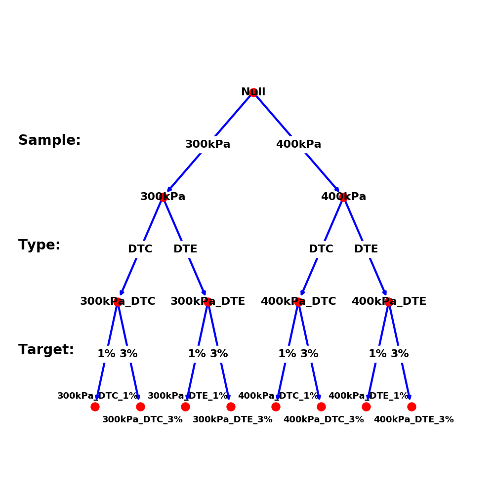
The decision trees are constructed based on a hierarchical series of test conditions (e.g., category of test, pressure level, target strain level) that an experimentalist needs to decide in order to design an experiment on a material. Assuming that an experiment can be completely and uniquely defined by an ordered list of selected test conditions , where is the total number of test conditions. Each is selected from a finite set of choices , where is the number of choices for the th test condition. For test conditions with inherently continuous design variables, can include preset discrete values. For example, the target strain for a loading can be chosen from discrete values of , , , etc. All design choices available to experimentalists are represented by an ordered list of sets with a hierarchical relationship such that, if , must be selected prior to the selection of .
After the construction of for experimentalists, a decision tree is built top-down from a root node representing the ’Null’ state that no test condition is decided. The root node is split into subnodes according to the first level of decisions . Each subnode is further split into subnodes according to the second level of decisions . The splitting process on the subnodes is carried out recursively for all the levels of decisions in . Finally, the down-most leaf nodes represent all possible combinations of test conditions. The maximum number of possible configurations of experiments is , when all decisions across are independent. The number of possible experiments is reduced () when restrictions are specified for the selections of test conditions. E.g., the selection of may prohibit the selections of certain choices in subsequent test conditions . The experimentalists can choose multiple experiments by taking multiple paths in the decision tree from the root node to the leaf nodes. The total number of possible combination of paths, if the maximum allowed number of simultaneously chosen paths is , is , where is the combination number.
Example for hierarchical test conditions and experimental decision tree.
Consider a simple design of mechanical experiments for geomaterials, for which all choices are listed in
| (1) |
The first decision is to pick the initial geomaterial sample to test. Assuming that a sample is fully characterized by its initial pressure , a simple set of discrete sample choices is given as
| (2) |
The second test condition is the type of the experiment. The experiment can be either drained triaxial compression test (’DTC’) or drained triaxial extension test (’DTE’). Then
| (3) |
The third test condition to decide is the target strain magnitude for the loading. For example,
| (4) |
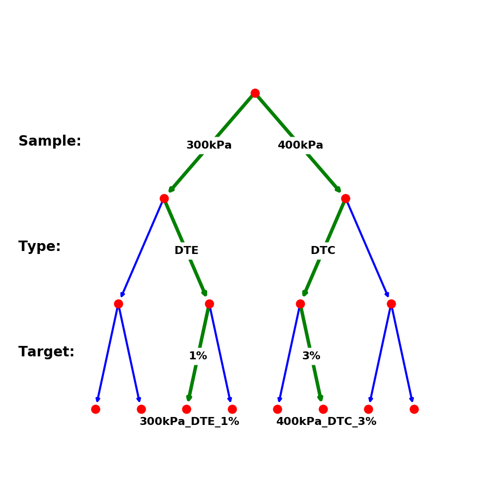
After all three decisions are sequentially made (taking a path in the decision tree), the experiment is completely determined by an ordered list, e.g., . It indicates that the AI experimentalist decides to perform a monotonic drained triaxial extension test on a sample with until the axial strain reaches .
The decision tree for the hierarchical design of geomaterial experiments specified by Equations (1), (2), (3), (4) is shown in Fig. 1(a). The vertex sets and edge sets of the graph are
| (5) | ||||
In this example, . If an experimentalist only collects data from one or two experiments, i.e., , the total number of possible combinations is . Fig. 1(b) presents two example paths with edge labels illustrating the hierarchical decisions on the test conditions in order to arrive at the final experimental designs ’300kPa_DTE_1%’ and ’400kPa_DTC_3%’.
∎
In this section, we present two decision trees for the design of geomechanical experiments, one for the bulk mechanical behavior of granular materials, another for the traction-separation behaviour of granular interfaces. We later study the intelligence of the reinforcement-learning-based experimentalists (protagonist and adversary) on these decision trees in Section 5.
2.1 Decision tree for AI-guided experimentation on bulk granular materials
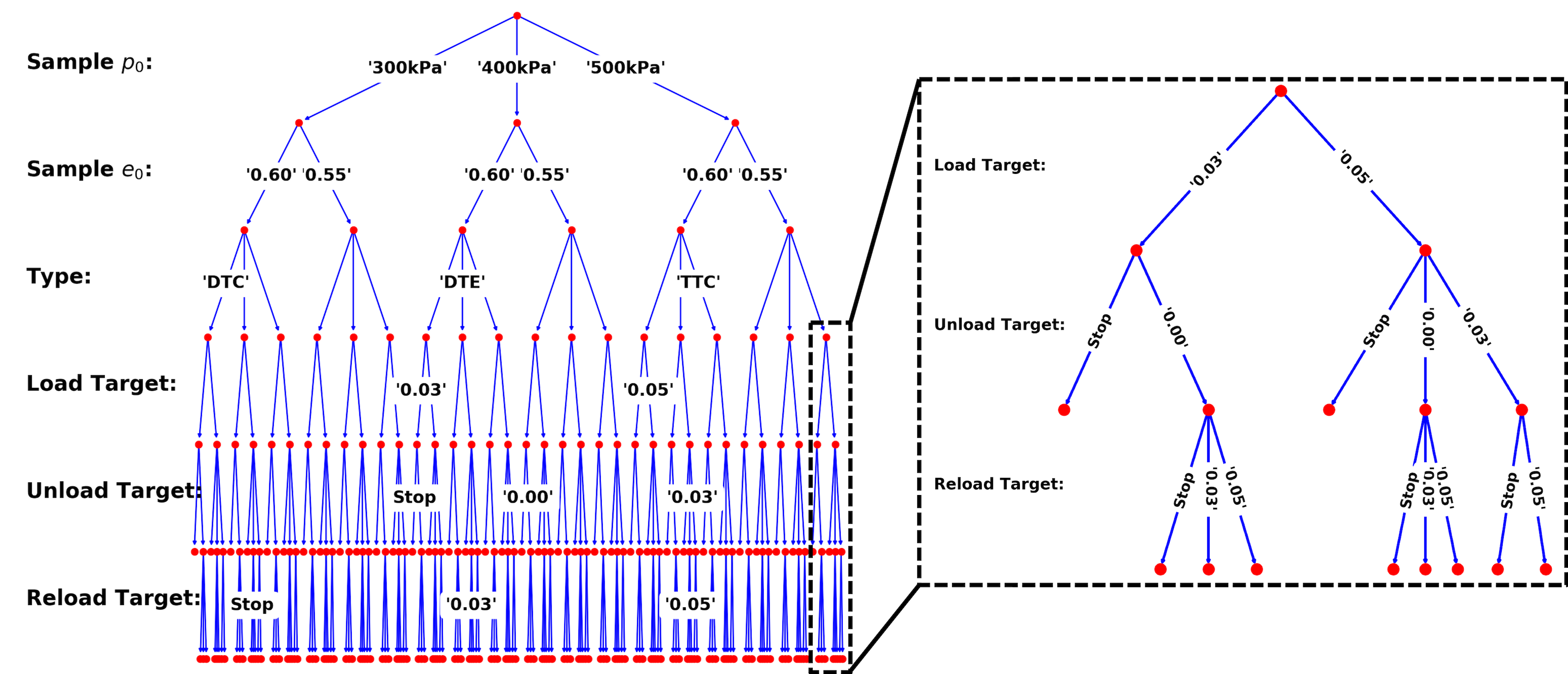
This section defines a representative decision tree for the AI-guided experimentation on bulk geomaterials. The hierarchical series of test conditions includes six elements, = [, , , , , ], such that the AI experimentalists can choose isotropic granular samples of different initial pressure and initial void ratio , perform different drained triaxial tests, and design different loading-unloading-reloading paths.
The choices for each test conditions are shown in Table 1, represented by decision labels. The decision labels for the test types are defined as follows,
-
1.
’DTC’: drained conventional triaxial compression test (, ),
-
2.
’DTE’: drained conventional triaxial extension test (, ),
-
3.
’TTC’: drained true triaxial test with (, , ),
with the loading conditions represented by constraints on the components of the stress rate and strain rate tensors
| (6) |
Since ’DTC’ and ’DTE’ are special cases of true triaxial tests, the choices for are equivalent to choosing the value of from , respectively (Rodriguez and Lade, 2013).
The decision labels ’NaN’ in and indicate that the unloading or reloading is not activated. This design enables the freedom of generating monotonic loading paths (e.g., ’5%_NaN_NaN’), loading-unloading paths (e.g., ’5%_0%_NaN’) and loading-unloading-reloading paths (e.g., ’5%_0%_3%’). There are restrictions in choosing the strain targets. The experimentalist picks the loading target in first and the unloading target in must be, if not ’NaN’ (stop the experiment), smaller than the loading strain. Then the reloading target in must be, if not ’NaN’, larger than the unloading strain.
| Test Conditions | Choices |
|---|---|
| ’Sample ’ | |
| ’Sample ’ | |
| ’Type’ | |
| ’Load Target’ | |
| ’Unload Target’ | |
| ’Reload Target’ |
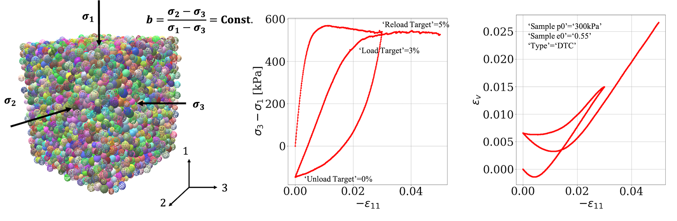
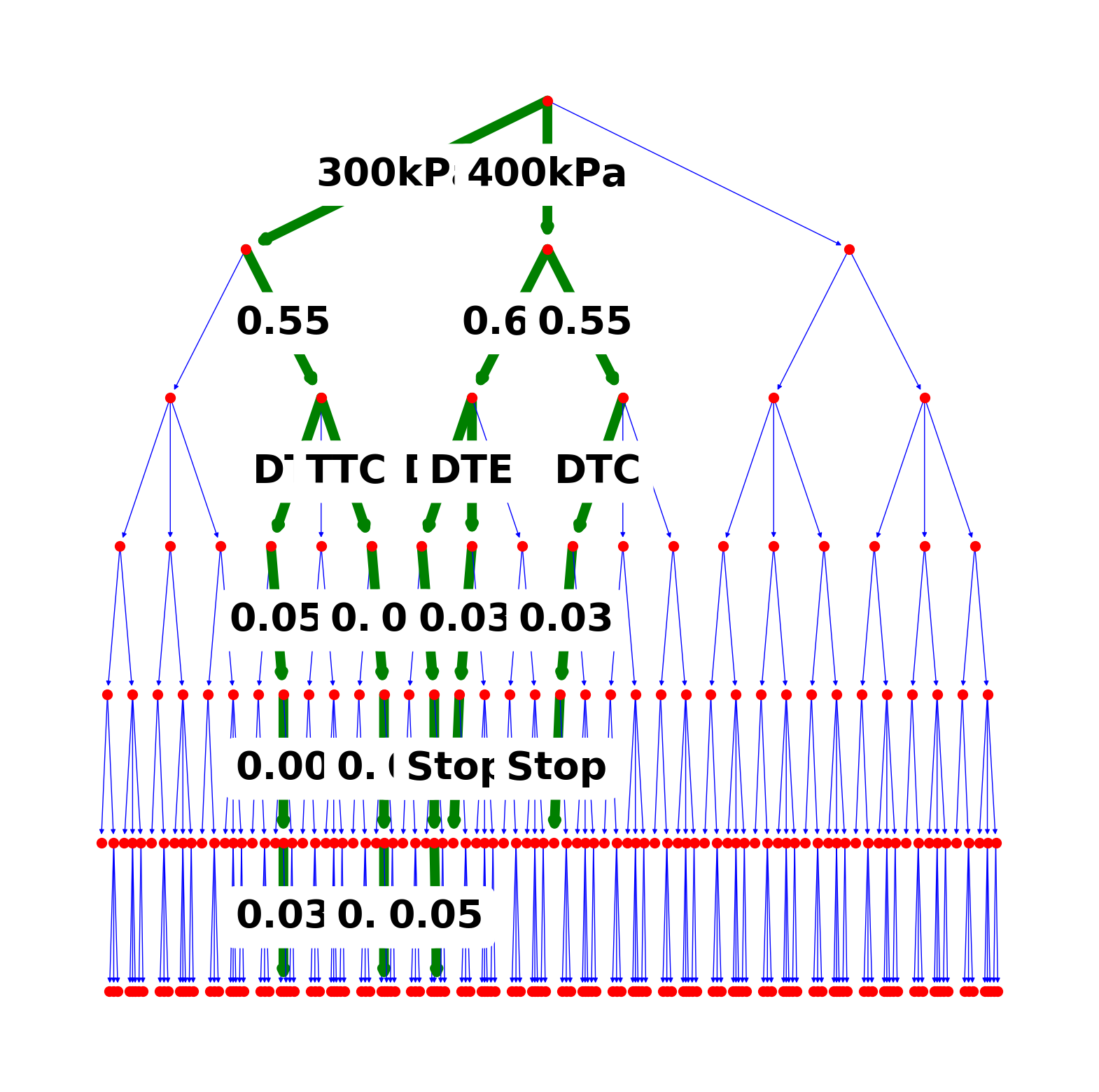
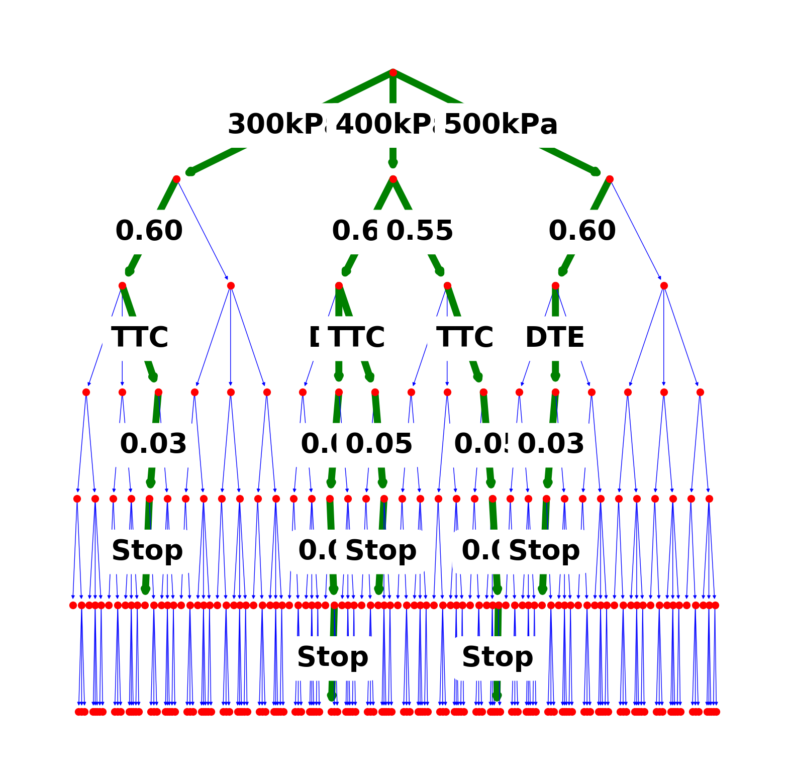
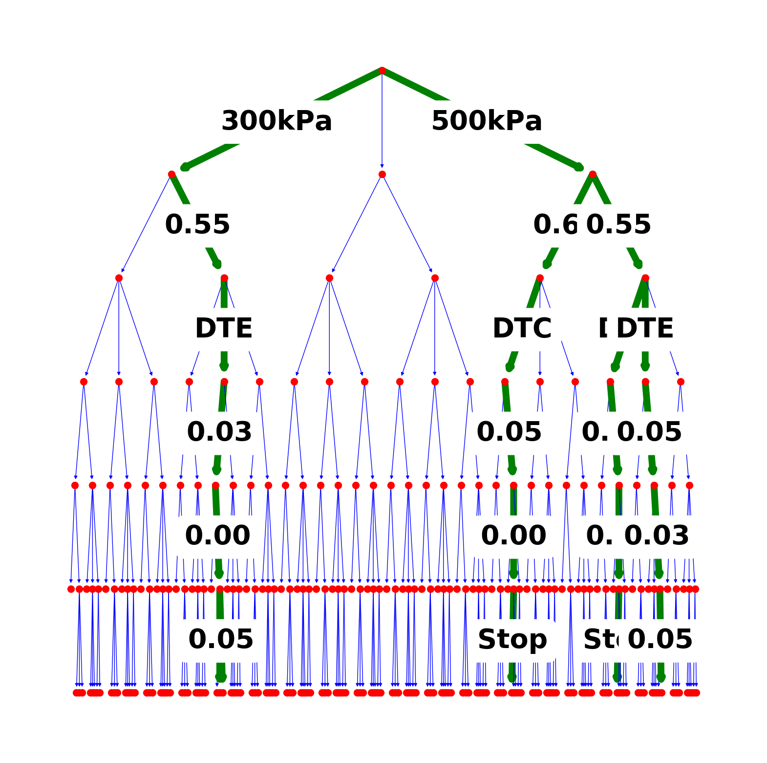
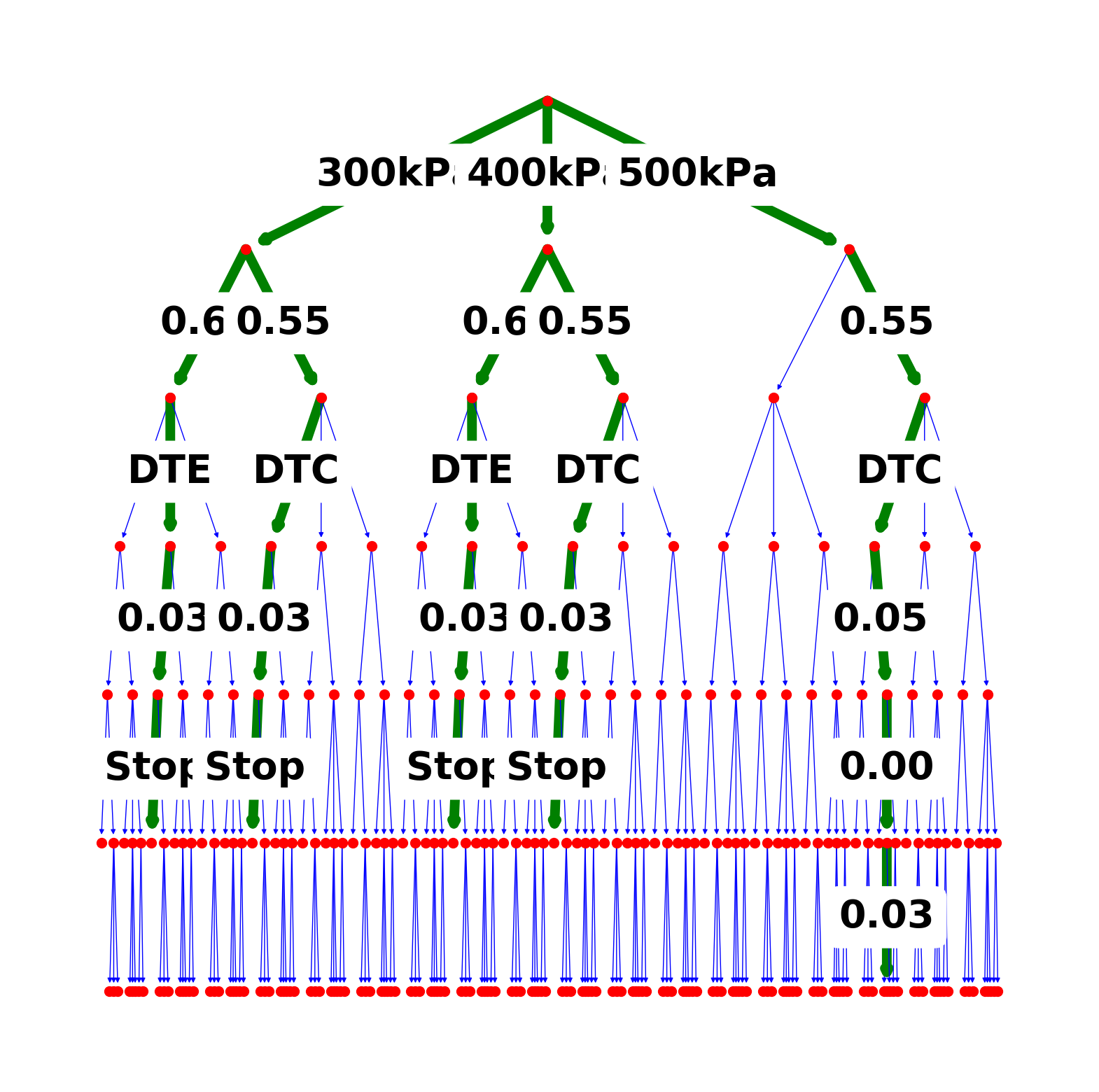
The corresponding decision tree is shown in Fig. 2. The subtree concerning the restricted decision-making in , and is also detailed in the figure. The total number of experimental designs (which equals to the number of leaf nodes in the tree) is . Fig. 3 provides the experimental settings on DEM (discrete element methods) numerical specimens and data from one example of the experiments. The total number of experimental data combinations increases significantly when the maximum allowed simultaneous paths increases. The combination number equals to when , equals to when , equals to when , etc.
2.2 Decision tree for AI-guided experimentation on granular interfaces
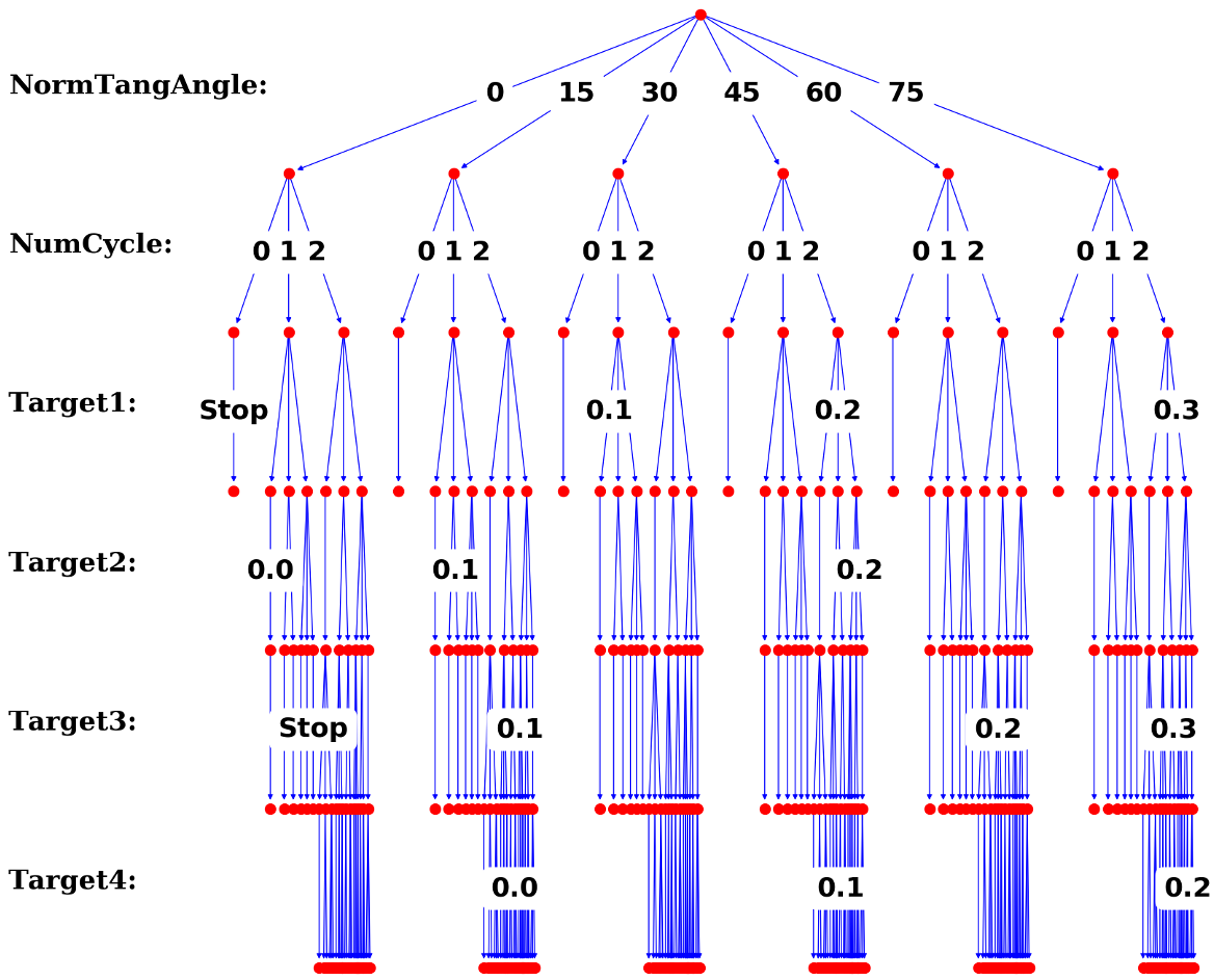
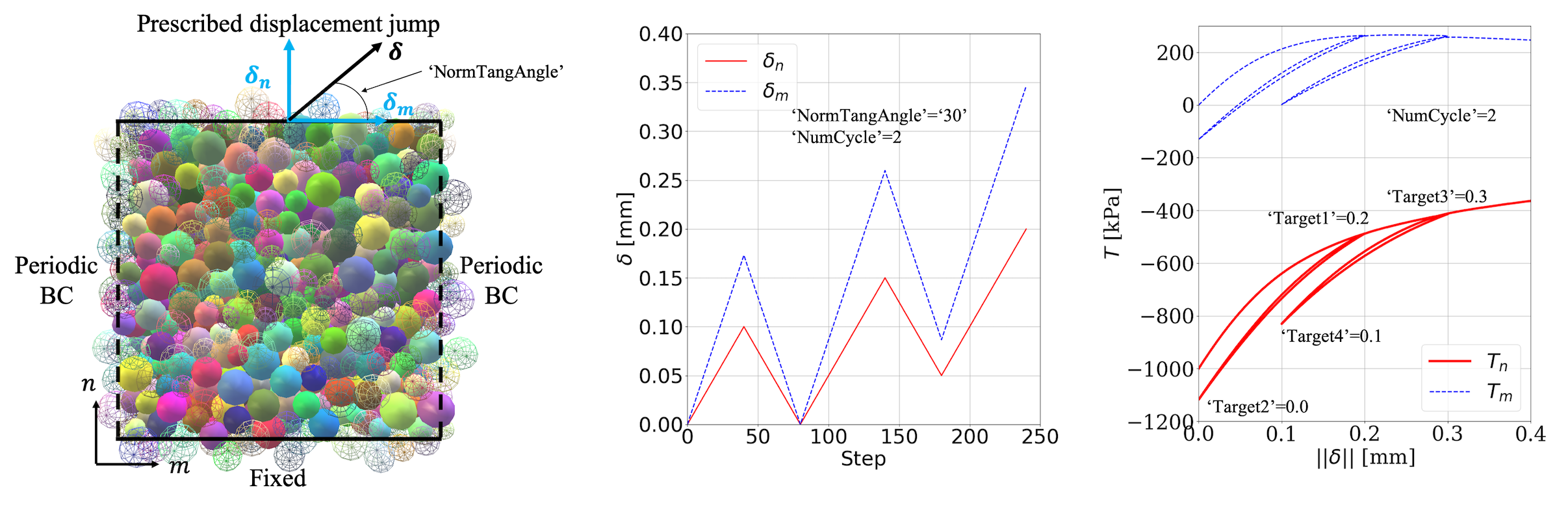
This section defines a representative decision tree for the AI-guided experimentation on granular interfaces. The hierarchical series of test conditions includes six elements, = [, , , , , ], such that the AI experimentalists can choose the direction of the prescribed displacement jump, the number of loading cycles, and different target displacement values to design complex loading paths.
The choices for each test conditions are shown in Table 2, represented by decision labels. ’NormTangAngle’ represents the angle between the displacement jump vector and the tangential direction vector, the corresponding values in the Choices column are in units of degree. ’NumCycle’ represents the number of loading-unloading cycles. The conditions ’Target1’, ’Target2’, ’Target3’, ’Target4’ represent the target displacement jump magnitudes along the loading-unloading cycles, the corresponding values in the Choices column are in units of millimeters. Regardless of the loading-unloading cycles, the final displacement jump reaches the magnitude of 0.4 mm. The decision label ’NaN’ indicates that the unloading or reloading is not activated. For example, ’NumCycle’=’0’ means a monotonic loading to 0.4 mm, hence all the target conditions should adopt the values of ’NaN’; ’NumCycle’=’1’ means a loading-unloading-reloading path to 0.4 mm, hence ’Target1’ (loading target) and ’Target2’(unloading target) can adopt values within , while ’Target3’ and ’Target4’ should be ’NaN’s.
| Test Conditions | Choices |
|---|---|
| ’NormTangAngle’ | |
| ’NumCycle’ | |
| ’Target1’ | |
| ’Target2’ | |
| ’Target3’ | |
| ’Target4’ |
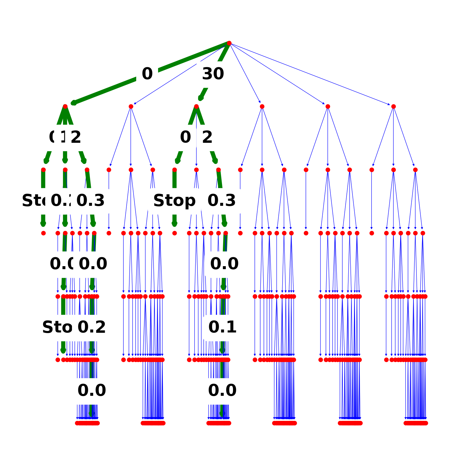
The corresponding decision tree is shown in Fig. 4. The total number of experimental designs (which equals to the number of leaf nodes in the tree) is . Fig. 5 provides the experimental settings on DEM (discrete element methods) numerical specimens and data from one example of the experiments. The total number of experimental data combinations, for example, equals to when . Such number is already impractical for human to find the optimal data sets for calibration and falsification by trial and error. For high efficiency, the decisions in performing experiments should be guided by experienced experts or, in this paper, reinforcement-learning-based AI.
3 Multi-agent non-cooperative game for model calibration/falsification with adversarial attacks
This section presents the design of a data acquisition game for both AI experimentalists (protagonist and adversary) to play, based on the decision trees defined in Section 2 involving the common actions in testing the mechanical properties of geomaterials. The goal of this game is to enable the protagonist agent to find the optimal design of experiments that best calibrate a constitutive law, while having the adversary agent designs a counterpart set of experiments that expose the weakness of the models in the same decision tree that represents the application range. For simplicity, we assume that all experiments conducted by both agents are fully reproducible and free of noise. We will introduce a more comprehensive treatment for more general situations in which the bias and sensitivity of the data as well as the possibility of erroneous and even fabricated data are considered in future. Such a treatment is, nevertheless out of the scope of this work.
Multi-agent multi-objective Markov games (Littman, 1994) have been widely studied and applied in robotics (Pinto et al., 2017), traffic control (Wiering, 2000), social dilemmas (Leibo et al., 2017), etc. In our previous work, Wang et al. (2019), our focus was on designing agents that have different actions and states but share the same goal. In this work, our new innovation is on designing a zero-sum game in which the agents are competing against each other for a pair of opposite goals. While the reinforcement learning may lead to improved game play through repeated trial-and-error, the non-cooperative nature of this new game will force the protagonist to act differently in response to the weakness exposed by the adversary. This treatment therefore may lead to a more robust and regularized model. In this work, the protagonist and the adversary are given the exact same action space mathematically characterized as a decision tree. While a non-cooperative game with non-symmetric action spaces can enjoy great performance as demonstrated in some of the OpenAI systems (Pinto et al., 2017), such an extension is out of the scope of this study and will be considered in the future.
3.1 Non-cooperative calibration/falsification game involving protagonist and adversary
We follow the general setup in Pinto et al. (2017) to create a two-player Markov game with competing objectives to calibrate and falsify a constitutive model. Both calibration and falsification are idealized as procedures that involves sequences of actions taken to maximize (in the case of calibration) and minimize (in the case of the falsification) a metric that assesses the prediction accuracy and robustness.
Consider the Markov decision process (MDP) in this game expressed as a tuple where is the set of game states and is the initial state distribution. is the set of actions taken by the protagonist in charge of generating the experimental data to calibrate a given material model. is the set of actions taken by the adversary in charge of falsifying the material model. is the transition probability density. and are the rewards of protagonist and adversary, respectively. If , the game is fully cooperative. If , the game is zero-sum competitive. At the current state of the game, if the protagonist is taking action sampled from a stochastic policy and the adversary is taking action sampled from a stochastic policy , the reward functions are and .
In this work, all the possible actions of the protagonist and the adversary agent are mathematically represented by decision trees (Section 2). The protagonist first selects one or more paths in its own tree which provide the detailed experimental setups to generate calibration data for the material model, then the adversary selects one or more paths in its own tree (identical to the protagonist’s tree) to generate test data for the calibrated model, aiming to find the worst prediction scenarios. The rewards are based on the prediction accuracy measures SCORE of the constitutive model against data. This measure of ’win’ or ’lose’ is only available when the game is terminated, similar to Chess and Go (Silver et al., 2017b, a), thus the final rewards are back-propagated to inform all intermediate rewards and . is defined to encourage the increase of SCORE of model calibrations, while is defined to favor the decrease of SCORE of forward predictions. In this setting, the game is non-cooperative, and generally not zero-sum.
3.2 Components of the game for the experimentalist agents
The agent-environment interactive system (game) for the experimentalist agents consists of the game environment, game states, game actions, game rules, and game rewards (Bonabeau, 2002; Wang and Sun, 2019) (Fig. 6). These key ingredients are detailed as follows.
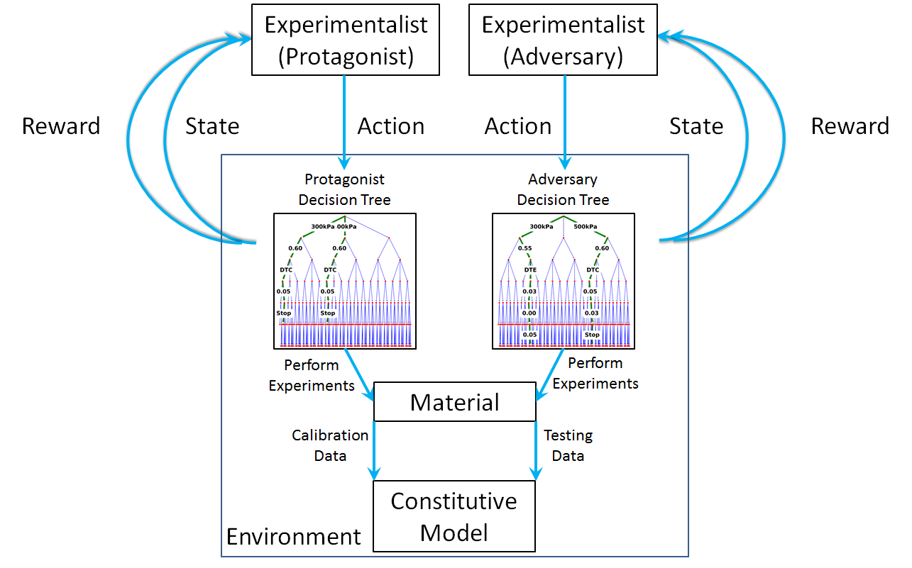
Game Environment consists of the geomaterial samples, the constitutive model for performance evaluation, and the experimental decision trees. The samples in this game are representative volume elements (RVEs) of virtual granular assemblies modeled by the discrete element method (DEM) (e.g., Fig. 3, Fig. 5). The preparation of such DEM RVEs are detailed in the numerical examples. The constitutive model can be given by the modeler agent in a meta-modeling game (Wang and Sun, 2019; Wang et al., 2019). In this paper, we focus on the interactive learning of data acquisition strategies for a certain constitutive model of interest. Three-agent protagonist-modeler-adversary reinforcement learning games is out of the scope of the current study. The protagonist and adversary agents determine the experiments on the RVEs in order to collect data for model parameter identification and testing the forward prediction accuracy of the constitutive model, respectively, via taking paths in their own decision trees (e.g., Fig. 1, Fig. 2, Fig. 4).
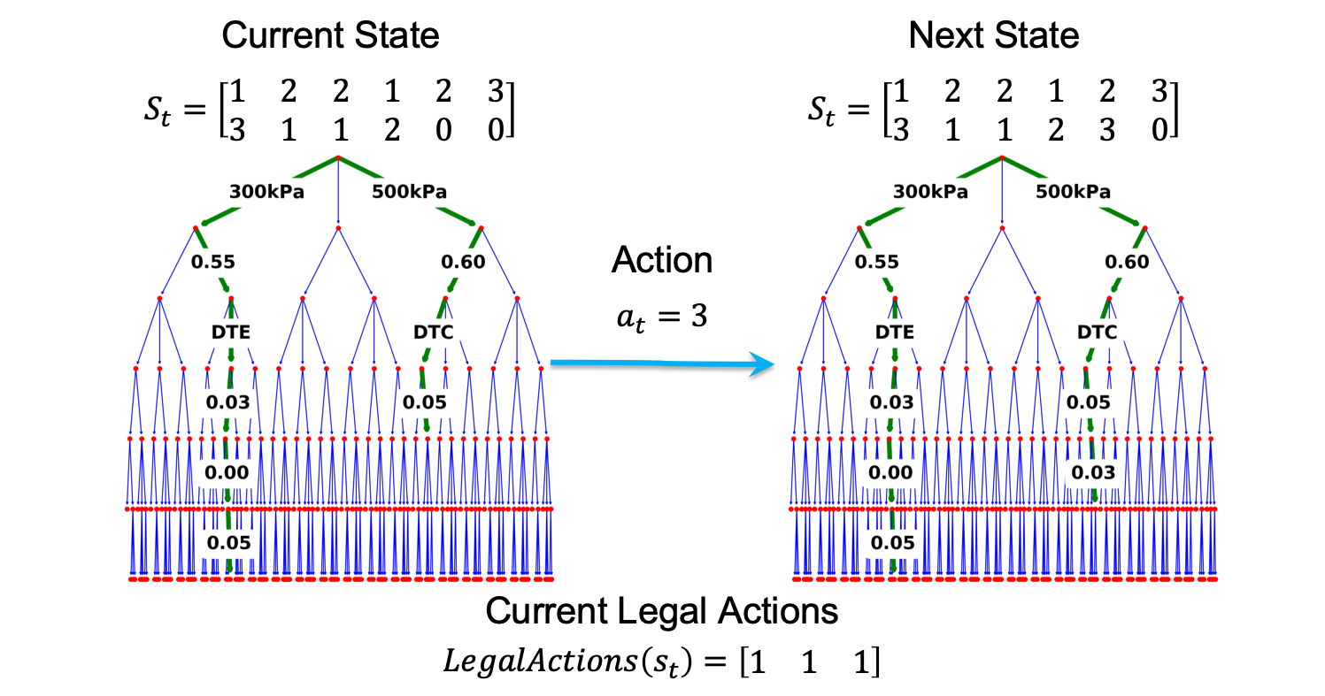
Game State For the convenience of deep reinforcement learning using policy/value neural networks, we use a 2D array to concisely represent the paths that the protagonist or adversary has selected in the experimental decision tree. The mapping from the set of the 2D arrays to the set of path combinations in the decision tree is injective. The array has a row size of and a column size of . Each row represents one path in the decision tree from the root node to a leaf node, i.e., a complete design of one experiment. The number of allowed experiments is restricted by the row size , which is defined by the user. Each array entry in the columns represents the selected decision label of each test condition in . The entry (integer) in the th row and th column indicates that the th decision label in the set is selected for the th experiment. Before the decision tree selections, the agent first decide a 1D array of size , with its th entry indicating whether the agent decides to take a new path in the decision tree (perform an another experiment) after the current th experiment is done. A value of 1 indicates continuation and 2 indicates stop. The total state of the game combines and , with flattened to a 1D array of size and then input into the policy/value neural networks for policy evaluations. Initially, all entries in the arrays are 0, indicating no decisions has been made.
Game Action The AI agent works on the game state arrays by changing the initial zero entries into integers representing the decision labels. The agent firstly selects 1 for continuation or selects 2 for stop in , in the left-to-right order. The agent then works on in the left-to-right then top-to-bottom order. Suppose that the first zero element of the current state array is in the th row and th column, the agent will select an integer (number of choices) to choose a decision label in . The size of the action space is .
Game Rule The AI agents are restricted to follow existing edges in the constructed decision tree, which has already incorporated decision limitations such as the choices of loading/unloading/reloading strain targets. The game rules are reflected by a list of binaries at the current state . If the th decision is allowed, the th entry is 1. Otherwise, the entry is 0. Figure 7 provides an example of the mathematical representations of the game states, actions and rules of the decision tree game.
Game Reward The rewards from the game environment to the experimentalists should consider the performance of a given constitutive model on calibration data and testing data. After the decision of experiments by the protagonist, these experiments are performed on material samples to collect data. Then the constitutive model is calibrated with these data, and the accuracy is evaluated by a model score . After the decision of experiments by the adversary, the calibrated constitutive model gives forward predictions on these testing data. The accuracy is evaluated by a model score . is returned to the protagonist to inform its game reward, while is returned to the adversary. This adversary attack reward system is the key to ensure that the protagonist generates calibration data to maximize the prediction strength of the constitutive model, while the adversary tries to explore the weakness of the model.
3.3 Evaluation of model scores and game rewards
The accuracy of model calibrations and forward predictions are quantified by calculating the discrepancy between the vector of data points and the vector of predicted values under the same experimental conditions. For both data points and predictions, , where is the data that falls into the th category of output features (quantities of interest, such as deviatoric stress and void ratio ). is the scaling operator (standardization, min-max scaling, …) for the th output feature.
The predictions come from a given constitutive model that is calibrated with data generated by the protagonist. In this work, for elasto-plastic models, the nonlinear least-squares solver ”NL2SOL” in Dakota software (Adams et al., 2014) is used to find the optimal parameter values. The initial guess, upper and lower bounds of each parameter are given by domain experts’ knowledge and preliminary estimations. For models of artificial neural networks, parameters are tuned by backpropagation algorithms using Tensorflow (Abadi et al., 2015). In both cases, the optimal material parameters minimize the scaled mean squared error objective function
| (7) |
The model scores measuring the prediction accuracy are based on the modified Nash-Sutcliffe efficiency index (Nash and Sutcliffe, 1970; Krause et al., 2005),
| (8) |
When , it recovers the conventional Nash-Sutcliffe efficiency index. Here we adopt , and
| (9) |
where and are maximum and minimum cutoff values of the modified Nash-Sutcliffe efficiency index, .
The game reward returned to the protagonist can consider both the calibration accuracy and the forward prediction accuracy, by including an exponential decay term:
| (10) |
where is the minimum N-S index observed in the gameplay history, is a user-defined decay coefficient. When , the decay term starts to drop the reward of the protagonist, otherwise . On the other hand, the game reward returned to the adversary is
| (11) |
Since the adversary is rewarded at the expense of the protagonist’s failure, it is progressively learning to create increasingly devastating experimental design to falsify the model, thus forcing the protagonist to calibrate material models that are robust to any disturbances created by the adversary. In this work, we refer to the move of the protagonist as calibration or defense, while the move of the adversary as falsification or attack.
4 Parallel reinforcement learning algorithm for the non-cooperative experimental/adversarial game
In the language of game theory, the meta-modeling game defined in the previous section is categorized as non-cooperative, asymmetric (the payoff of a particular strategy depends on whether protagonist or adversary is playing), non-zero-sum, sequential (the adversary is aware of the protagonist’s strategy in order to attack accordingly), imperfect information (the protagonist does not know how the adversary will attack). Let (, ) be a representation of this two-player (denoted by subscripts and ) non-cooperative game, with the set of strategy profiles. is the payoff (final reward) function evaluated at a strategy profile . A strategy profile is a Nash equilibrium if no unilateral change in by any player is more profitable for that player, i.e.,
| (12) |
The existence of at least one such equilibrium point is proven by Nash et al. (1950).
Solving the optimization problem directly to find the Nash equilibria strategies for this complex game is prohibitive (Perolat et al., 2015). Instead, deep reinforcement learning (DRL) algorithm is employed. In this technique the strategy of each player ( or ) is parameterized by an artificial neural network that takes in the description of the current state of the game and outputs a policy vector with each component representing the probability of taking actions from state , as well as a scalar for estimating the expected reward of the game from state , i.e.,
| (13) |
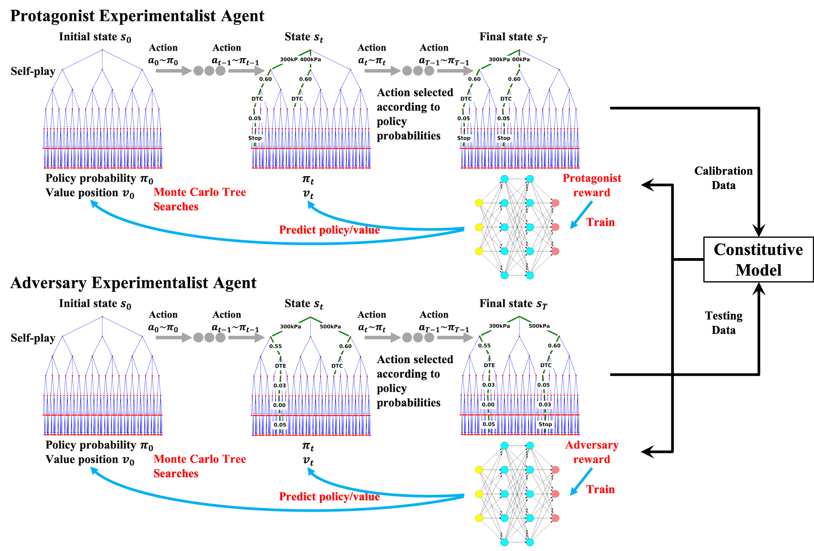
These policy/value networks provide guidance in learning optimal strategies of both protagonist and adversary in order to maximize the final game rewards. The learning is completely free of human interventions after the complete game settings. This tactic is considered one of the key ideas leading to the major breakthrough in AI playing the game of Go (AlphaGo Zero) (Silver et al., 2017b), Chess and shogi (Alpha Zero) (Silver et al., 2017a) and many other games. In Wang and Sun (2019), the key ingredients (policy/value network, upper confidence bound for Q-value, Monte Carlo Tree Search) of the DRL technique are detailed and applied to a meta-modeling game for modeler agent only, focusing on finding the optimal topology of physical relations from fixed training/testing datasets. Since DRL needs to figure out the optimal strategies for both agents, the algorithm is extended to multi-agent multi-objective DRL (Tan, 1993; Foerster et al., 2016; Tampuu et al., 2017). The AI for protagonist and adversary are improved simultaneously during the self-plays of the entire meta-modeling game, according to the individual rewards they receive from the game environment and the communications between themselves (Figure 8).
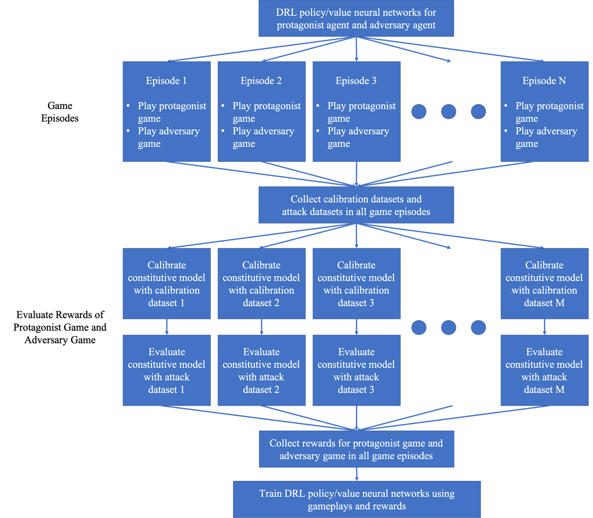
The pseudocode of the reinforcement learning algorithm to play the non-cooperative game is presented in Algorithm 1. This is an extension of the algorithm in (Wang and Sun, 2019). As demonstrated in Algorithm 1, each complete DRL procedure involves number of training iterations and one final iteration for generating the converged selected paths in decision trees. Each iteration involves number of game episodes that construct the training example set for the training of the policy/value networks and . For decision makings in each game episode, the action probabilities are estimated from runs of MCTS simulations.
The state values can be equal to the continuous reward functions (10), (11) to train the policy/value neural networks. To further improve the convergence rate of the DRL algorithm, we propose an empirical method to train the networks with binary state values (1 or -1) post-processed from the reward values, which is similar to the concept of ”win” (1) and ”lose” (-1) in the game of Chess. Consider the set of rewards of the games played in the th DRL iteration. The maximum reward encountered from Iteration 0 to the current Iteration , is . A minimum reward is chosen as . A reward range in Iteration is . A strategy is considered as a ”win” () when its reward , while it is a ”lose” () when . is a user-defined coefficient which influences the degree of ”exploration and exploitation” of the AI agents. Similarly, for the adversary agent, , and are collected for each protagonist strategy . Then an attack strategy corresponding to is considered as a ”win” () when its reward , while it is a ”lose” () when . The training examples for the policy/value neural networks are limited to the gameplays in the DRL iterations , where is a user-defined hyperparameter controlling the degree of ”forget” of the AI agents.
Another new contribution to the DRL framework is that we improve the computational efficiency of DRL by executing the mutually independent gameplays and reward evaluations in a parallel manner, instead of serial executions as in previous works (Wang and Sun, 2018, 2019; Wang et al., 2019). We use the parallel python library ”Ray” (Moritz et al., 2018) for its simplicity and speed in building and running distributed applications. The new workflow of parallel playing of game episodes in each training iteration for DRL is illustrated in Figure 9.
5 Automated calibration and falsification experiments
We demonstrate the applications of the non-cooperative game for automated calibration and falsification on three types of constitutive models. The material samples are representative volume elements (RVEs) of densely-packed spherical DEM particles. The decision-tree-based experiments are performed via numerical simulations on these samples. The preparation and experiments of the samples are detailed in Appendix A. The three constitutive models studied in this paper are Drucker-Prager model (Tu et al., 2009), SANISAND model (Dafalias and Manzari, 2004), and data-driven traction-separation model (Wang and Sun, 2018). Their formulations are detailed in Appendix B. The results shown in this section are representatives of the AI agents’ performances, since the policy/value networks are randomly initialized and the MCTS simulations involve samplings from action probabilities. The gameplays during DRL iterations may vary, but similar convergence performances are expected for different executions of the algorithm. Furthermore, the material calibration procedures, such as the initial guesses in Dakota and the hyperparameters in training of the neural networks, may affect the game scores and the converged Nash equilibrium points. Finally, since simplifications and assumptions are involved in the DEM samples, their mechanical properties differ from real-world geo-materials. The conclusions of the three investigated constitutive models are only on these artificial and numerical samples. However, the same DRL algorithm is also applicable for real materials, when the actions of the AI experimentalists can be programmed in laboratory instruments.
The policy/value networks are deel neural network in charge of updating the Q table that determines the optimal strategies. The design of the policy/value networks are identical for both agents in this paper. Both of them consist of one input layer of the game state , two densely connected hidden layers, and two output layers for the action probabilities and the state value , respectively. Each hidden layer contains 256 artificial neurons, followed by Batch Normalization, ReLU activation and Dropout. The dropout layer is a popular regularization mechanism designed to reduce overfitting and improve generalization errors in deep neural network (cf. Srivastava et al. (2014)). The dropout rate is 0.5 for the protagonist and 0.25 for the adversary. These different dropout rates are used such that the higher dropout rate for the protagonist will motivate the protagonist to calibrate the Drucker-Prager model with less generalization errors, while the smaller dropout rate will help the adversary to find the hidden catastrophic failures in response to a large amount of protagonist’s strategies. In addition, the non-cooperative game requires the hyperparameters listed in Table 3 to configure the game.
| Hyperparameters | Definition | Usage |
| Maximum number of decision tree paths chosen by the agents | Define the dimension of the game states | |
| Maximum cutoff value of the modified Nash-Sutcliffe efficiency index | See Eq. (9) | |
| Minimum cutoff value of the modified Nash-Sutcliffe efficiency index | See Eq. (9) | |
| Number of training iterations | Define DRL iterations for training policy/value networks | |
| Number of gameplay episodes in each training iterations | Define the amount of collected gameplay evidences | |
| Number of Monte Carlo Tree Search simulations in each gameplay step | Control the agents’ estimations of action probabilities | |
| Decay coefficient for the protagonist’s reward | See Eq. (10) | |
| Coefficient for determining ”win” or ”lose” of a game episode | Set the agents’ balance between ”exploration and exploitation” | |
| Number of gameplay iterations for training of the policy/value networks | Control the agents’ ”memory depth” | |
| Temperature parameter for training iterations | Set the agents’ balance between ”exploration and exploitation” | |
| Temperature parameter for competitative gameplays | Set the agents’ balance between ”exploration and exploitation” |
5.1 Experiment 1: Drucker-Prager model
The two-player non-cooperative game is played by DRL-based AI experimentalists for Drucker-Prager model. The formulations of the model are detailed by Eq. (14), (15), (16). The initial guesses, upper and lower bounds of the material parameters for Dakota calibration are presented in Table 5. The game settings are for both the protagonist and the adversary, , . Hence the combination number of the selected experimental decision tree paths in this example is where 180 is the total number of leaves in the decision tree and 5 is the maximum number of paths chosen by either agent. The hyperparameters for the DRL algorithm used in this game are , , , , , , , .
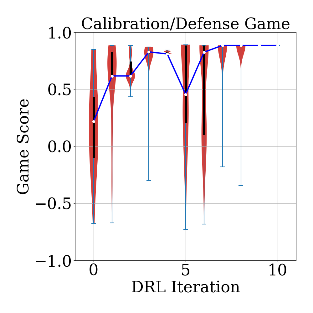
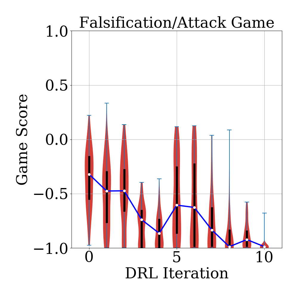
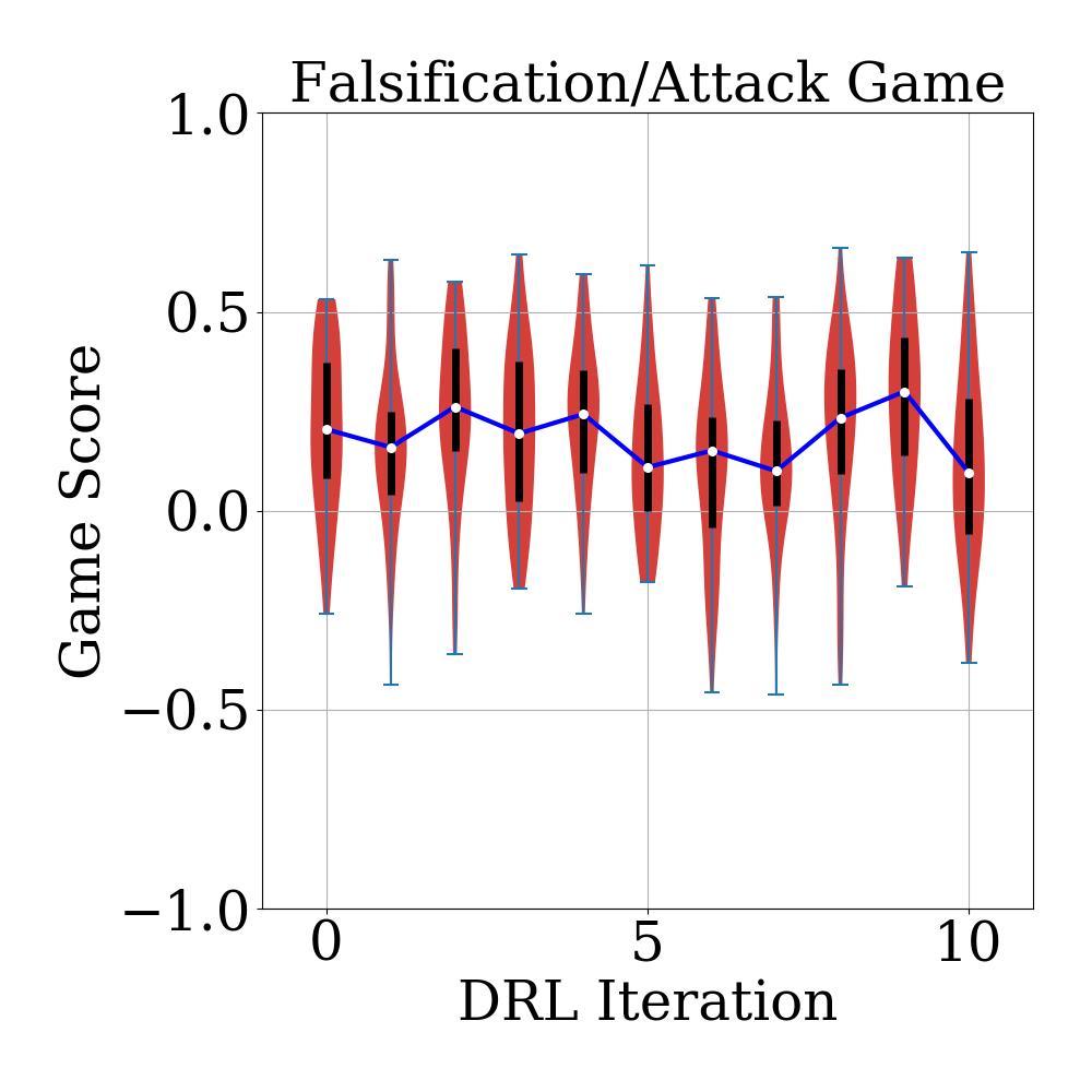
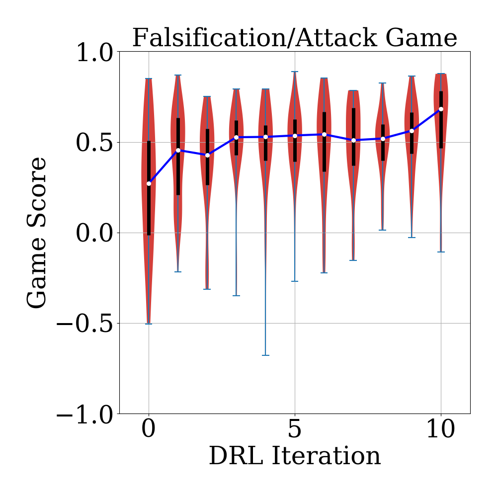
The statistics of the game scores played for the ”Calibration/Defense” by the protagonist and the ”Falsification/Attack” by the adversary during the DRL iterations are shown in Fig. 10. The AI agents only know the experimental decision tree and the rules of the two-player game without any prior knowledge on the strengths and weaknesses of the Drucker-Prager model. At the first DRL iteration, the agents play the game through trial and error guided by randomly initialized policy/value networks and MCTS. This lack of knowledge on proper gameplay strategies can be seen from the widely spread density distribution of game scores and the large inter-quantile range between 25% and 75% in both ”Calibration/Defense” and ”Falsification/Attack”. In the subsequent iterations, the agents progressively understand the ”winning strategies” via reinforcement learning on the gameplay histories and the associated game rewards, hence intend to play games with better outcomes. This is shown in the increase of the median of game scores by the protagonist and the decrease of the median by the adversary, and also the narrowing of inter-quantile ranges. In these intermediate training iterations, games can sometimes be played badly, since the agents are allowed to explore various game policies in order to avoid convergence to local extremum. The strengths of the AI agents after the 0th to 9th training iterations are tested by suppressing the ”exploration plays”, and the ultimate game scores show outstanding performances.
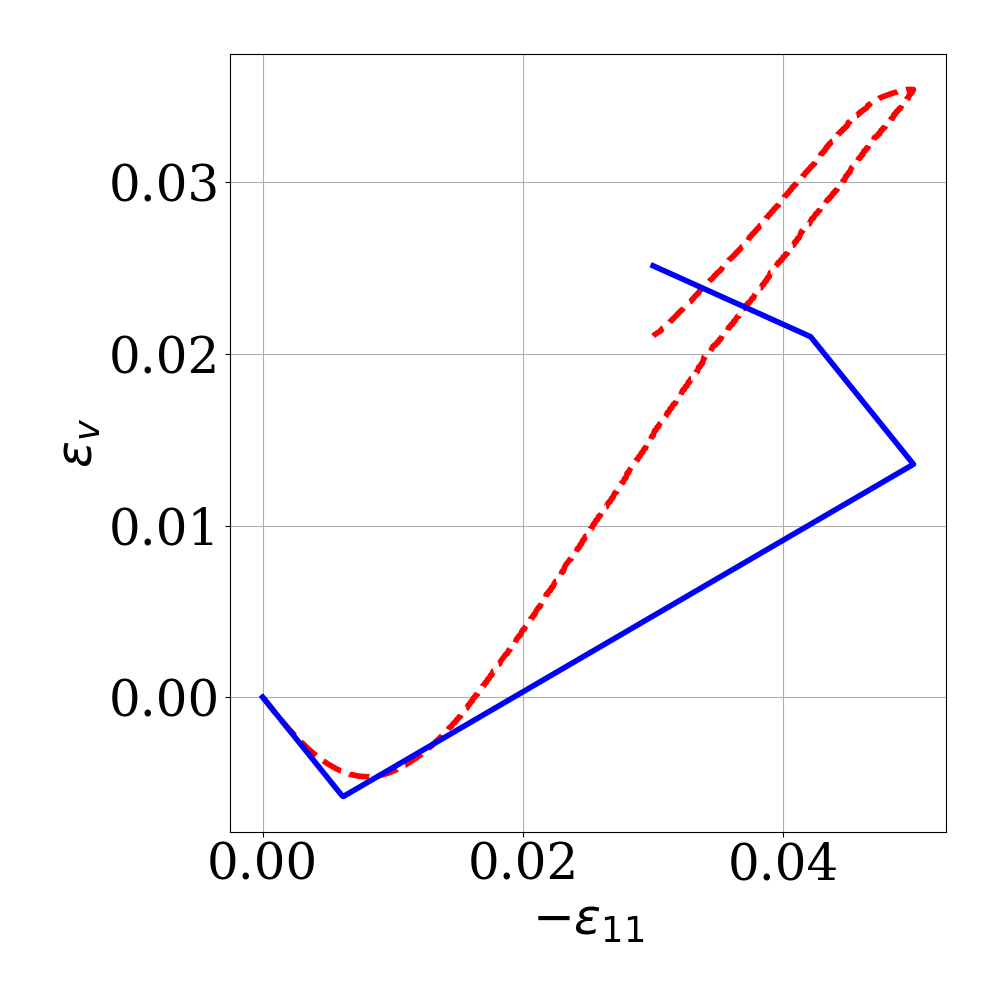
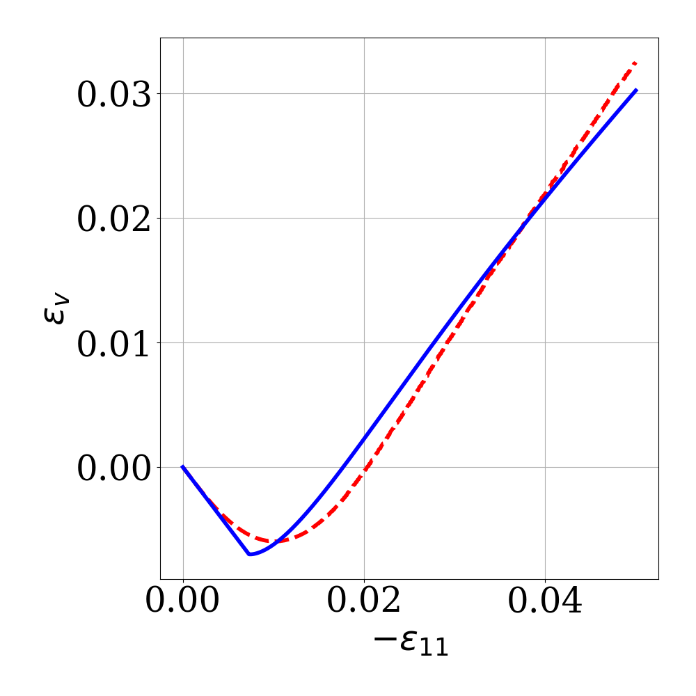
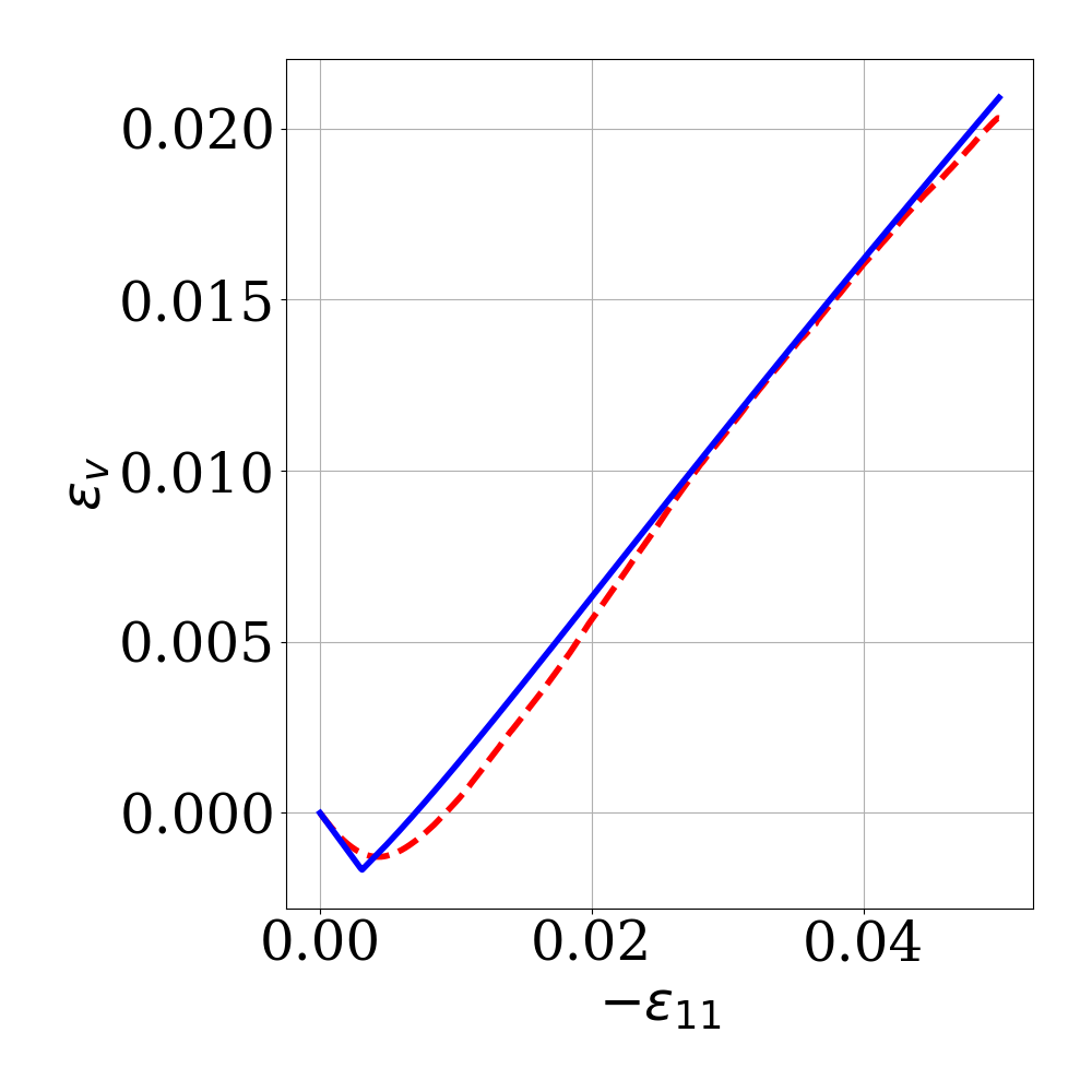
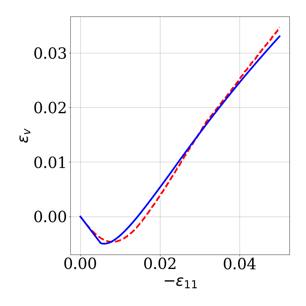
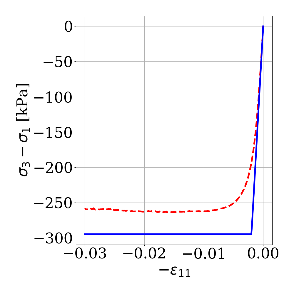
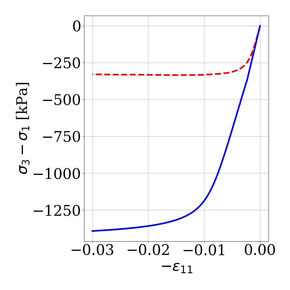
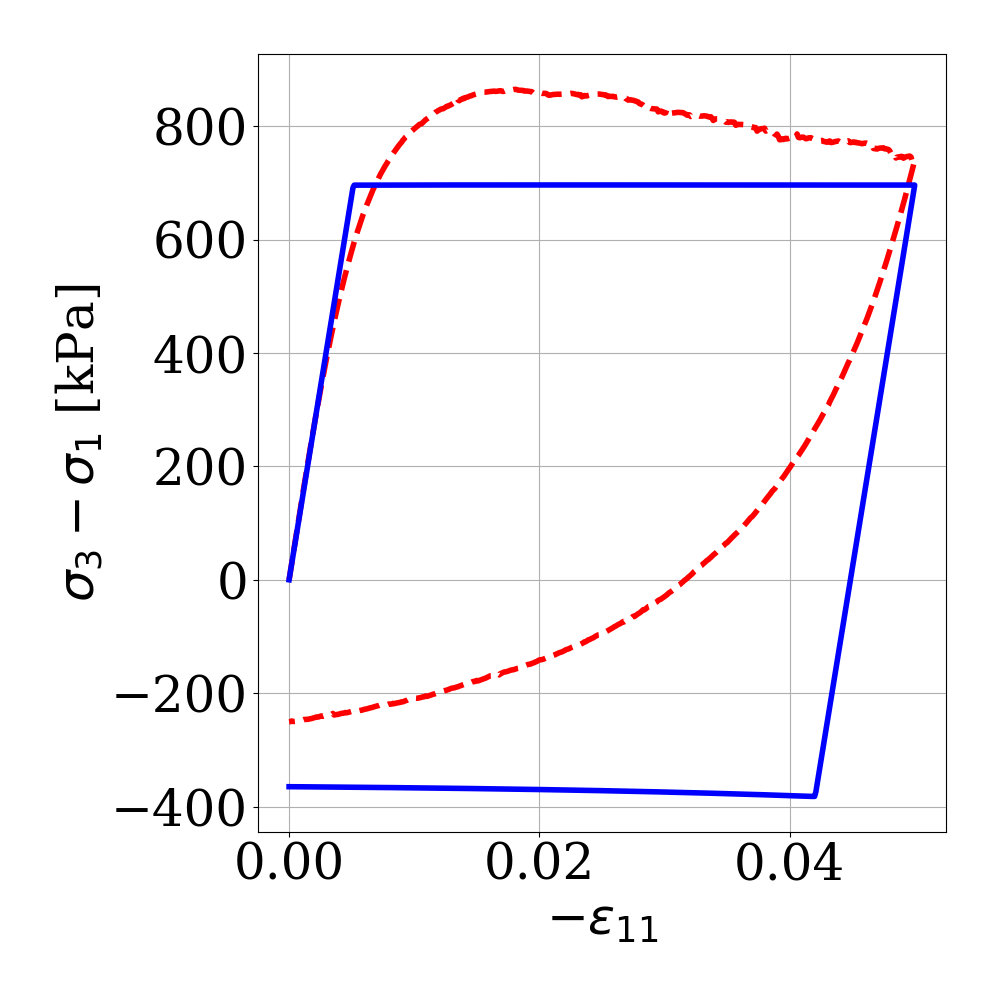
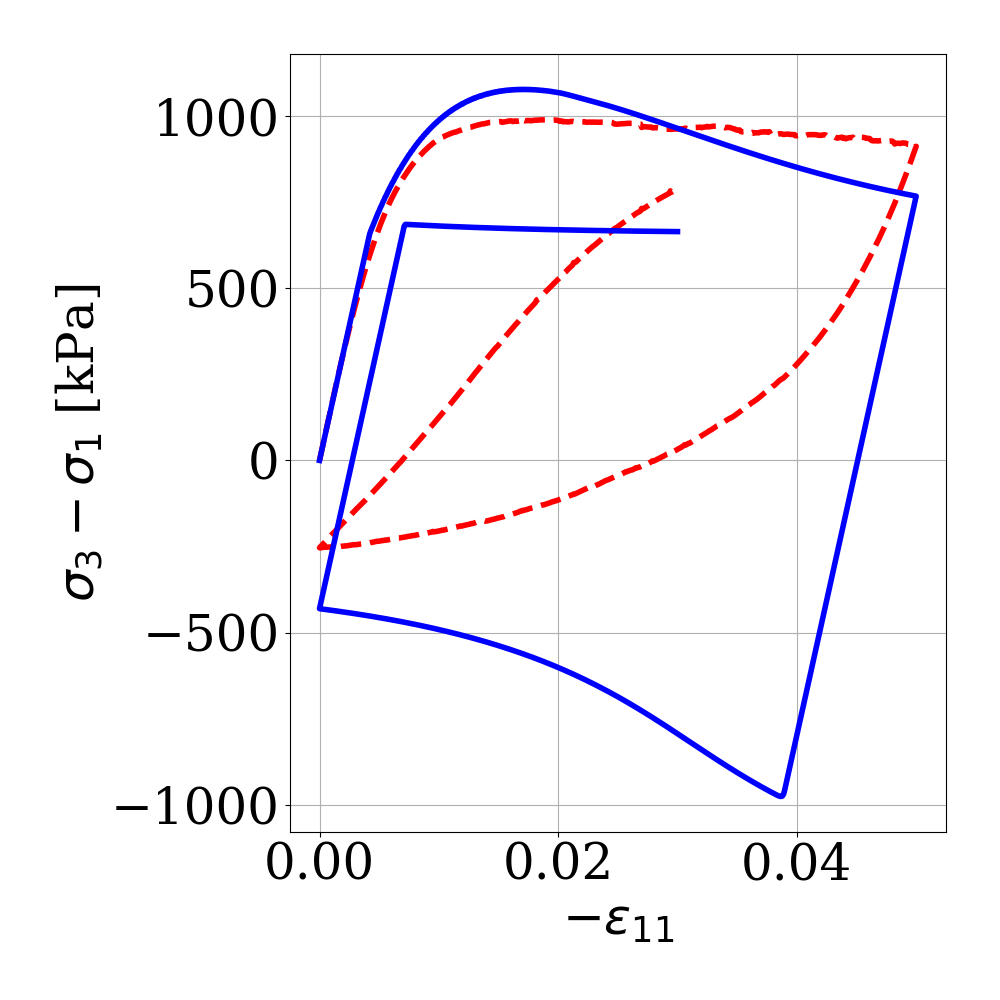
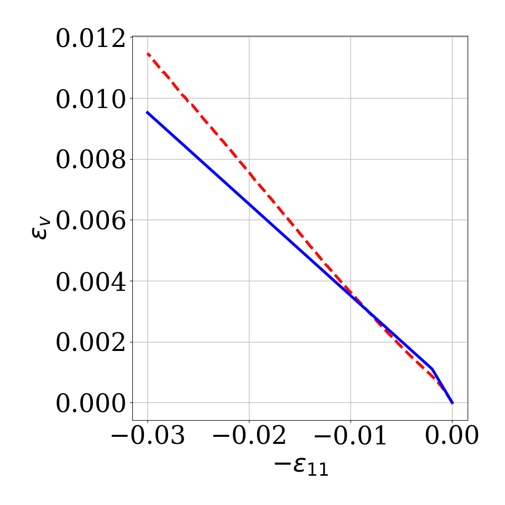
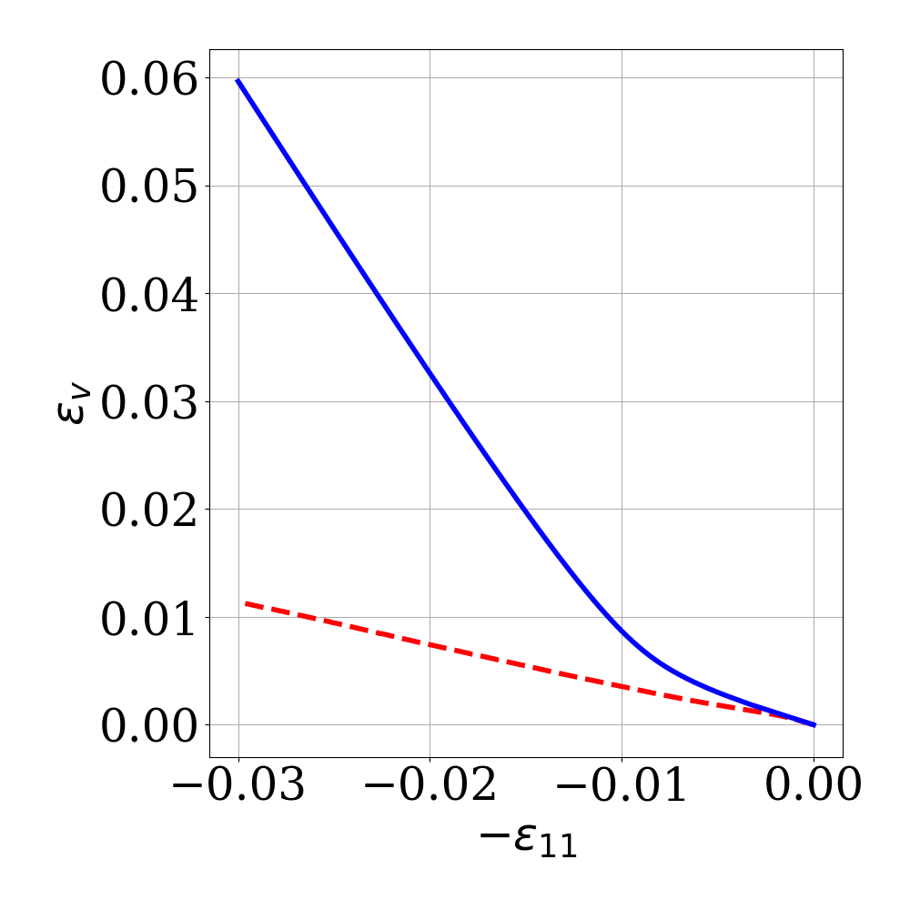
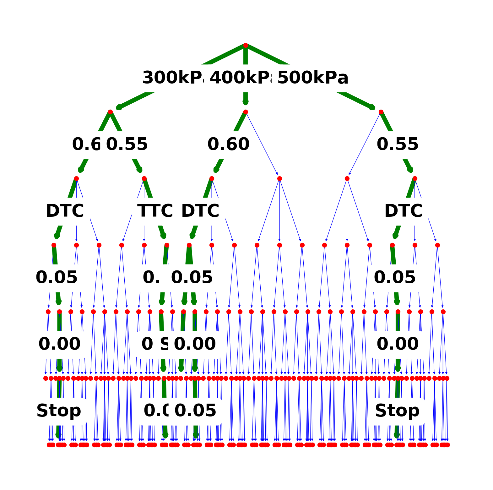
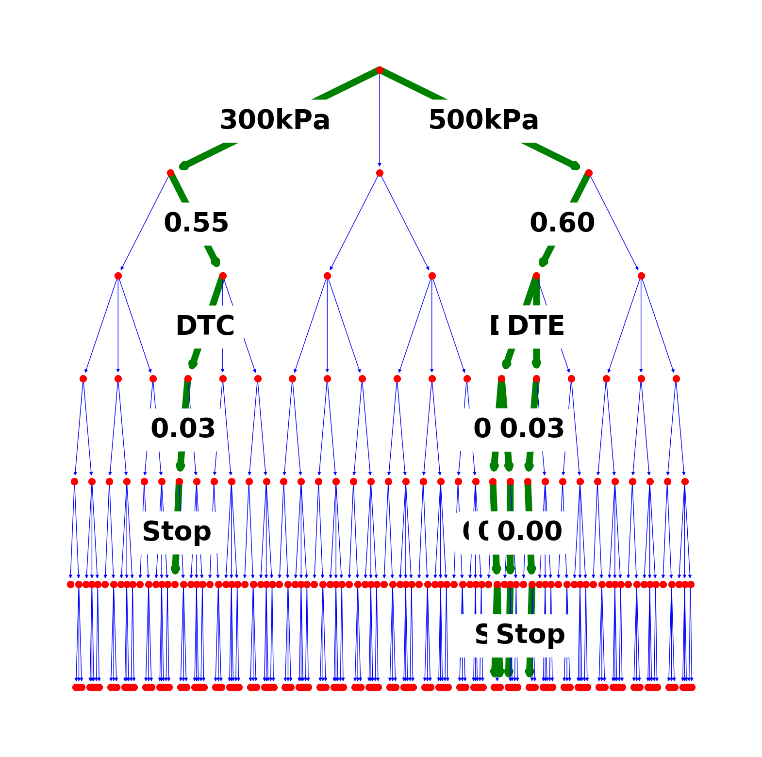
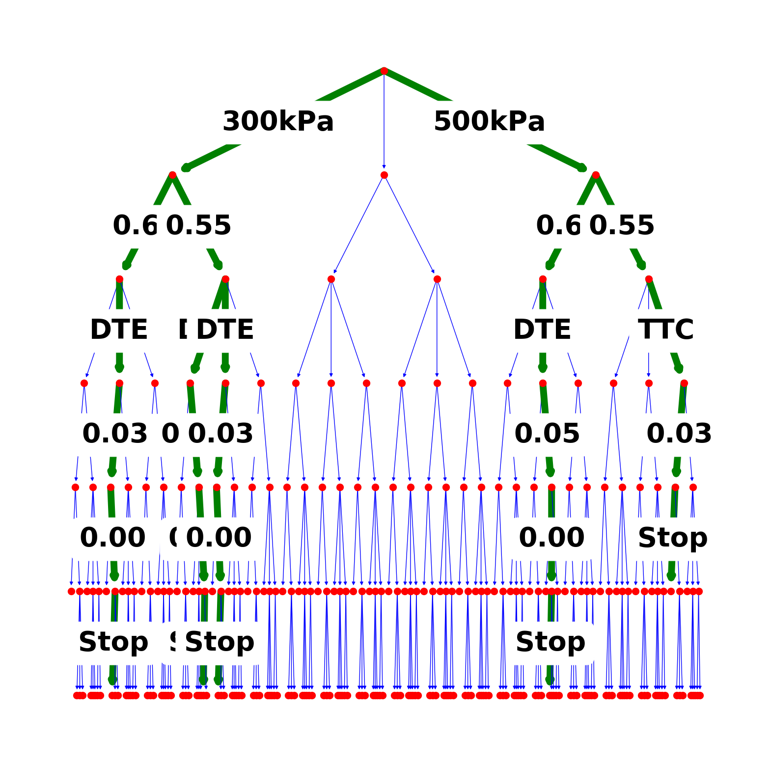
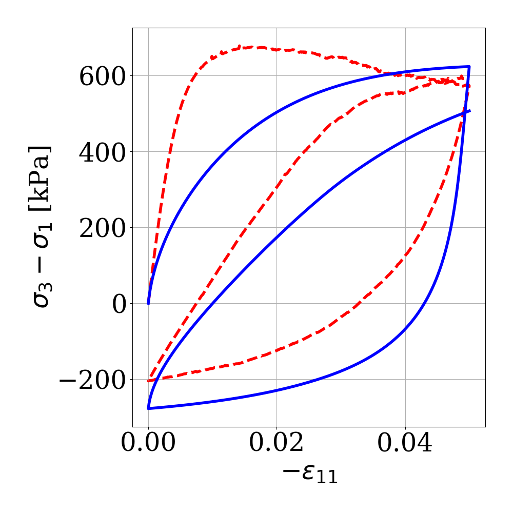
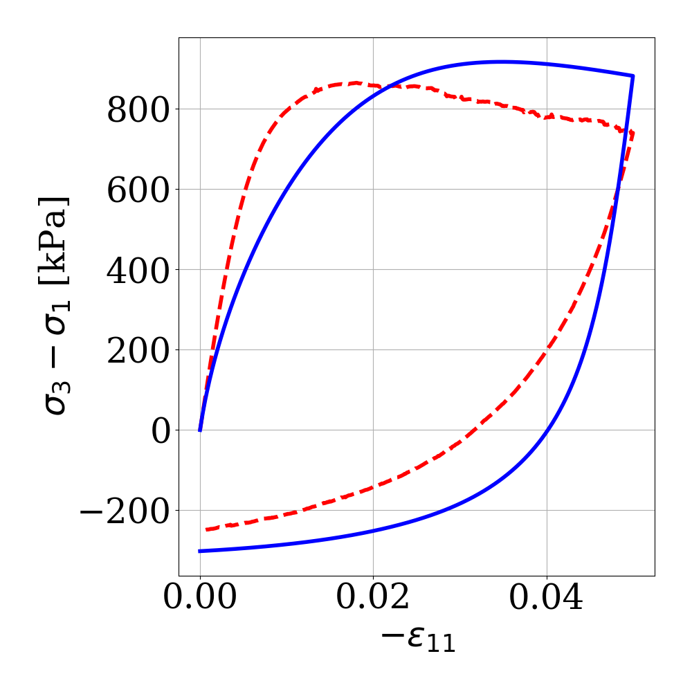
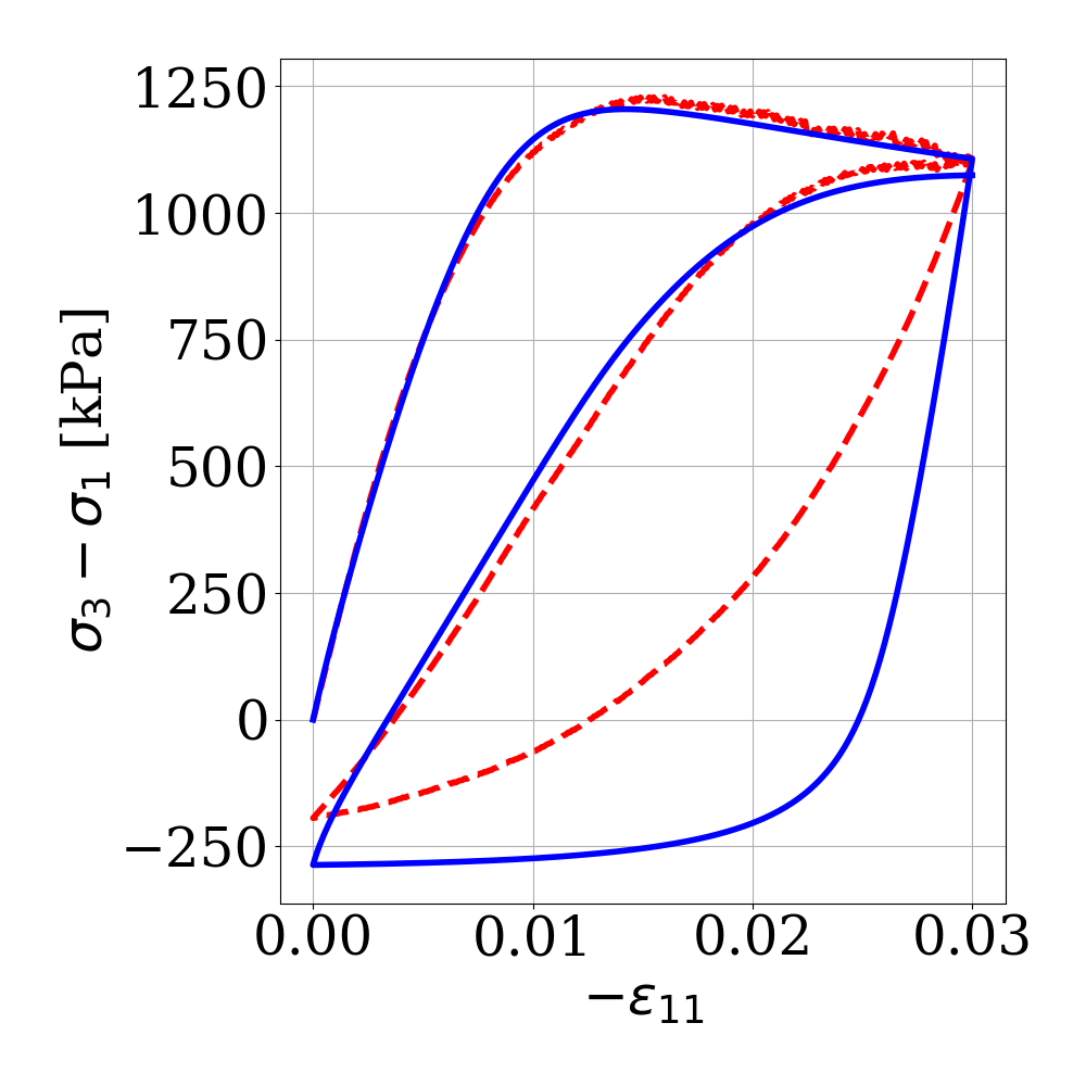
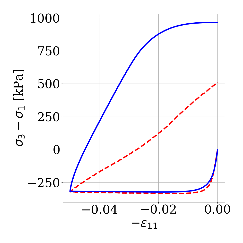
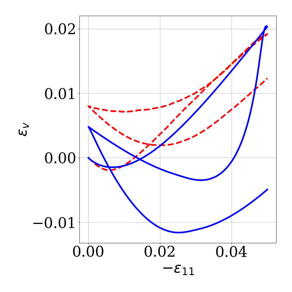
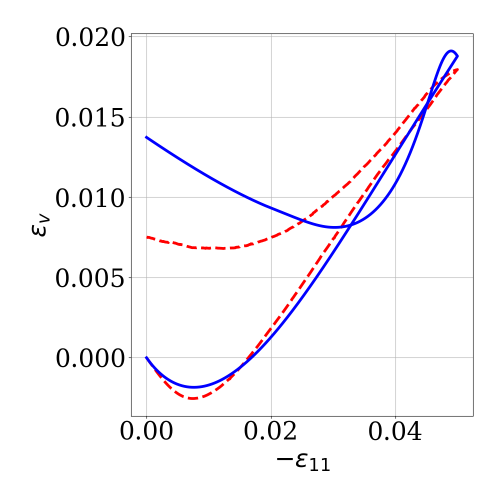
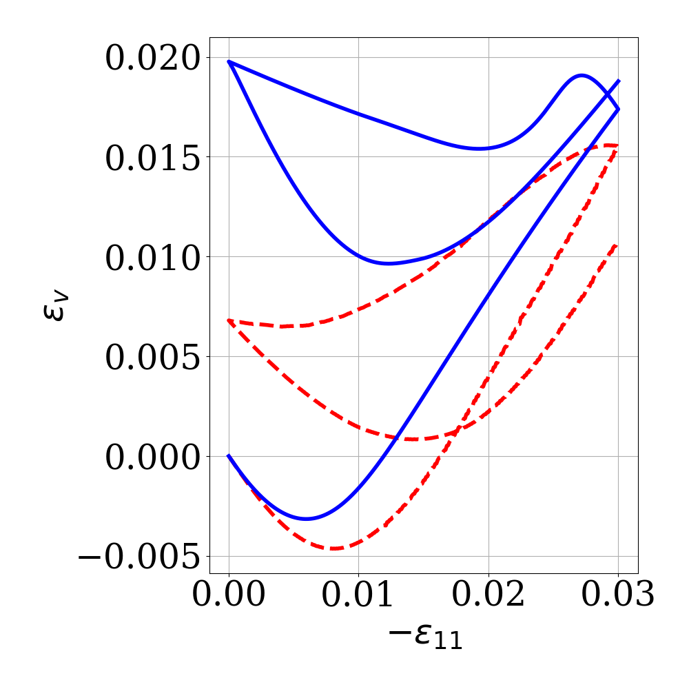
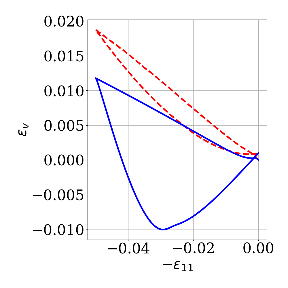
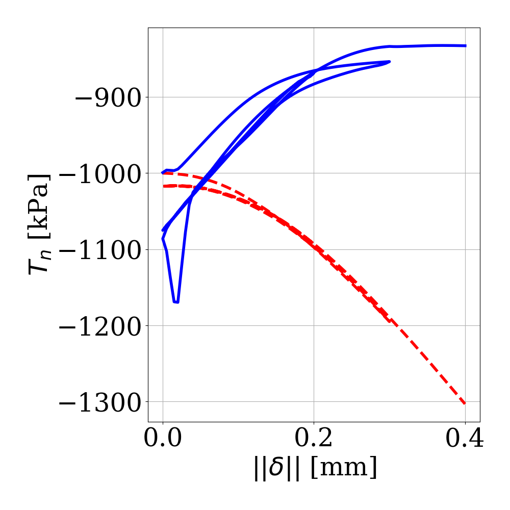
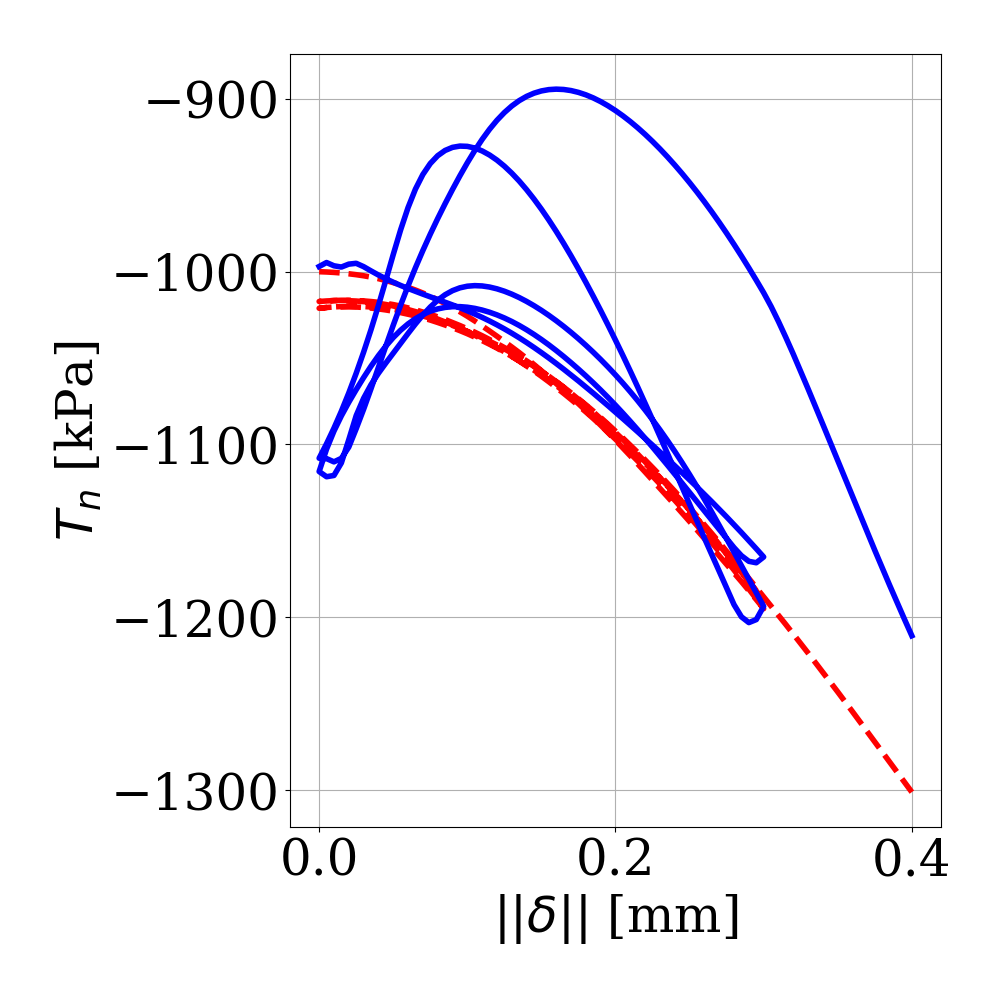
Examples of paths (experiments) selected by the protagonist during the DRL iterations are shown in Fig. 11. Based on all the evidences such as ones shown in these examples, the agent realizes that the Drucker-Prager model is not designed to simultaneously replicate data from samples with different initial confinement, initial void ratio, test types, and unloading-reloading paths. In the end, the agent concludes that the model is only accurate in modeling the mechanical behaviour of a single sample in TTC test with monotonic loading. Meanwhile, the adversary tries to attack the models calibrated by the protagonist using the experiments as shown in Fig. 12. The agent progressively comes to the conclusion that, when calibrated with monotonic TTC data, the model fails to predict DTC or DTE experiments on other samples with unloading-reloading. Fig. 13 and Fig. 14 give example response curves associated to the example decision tree paths shown in Fig. 11 and Fig.12, respectively. They illustrate the strength of the model in replicating the hardening-softening and contraction-dilation behavior of a densely compressed granular material. They also expose the model’s weakness in predicting the unloading-reloading behaviour, regardless of the calibration data. These conclusions on the Drucker-Prager model by the AI agents are consistent with the judgements from human experts, but they are drawn from the reinforcement learning on the two-player game without human knowledge.

Defense Game Score: 0.262

Defense Game Score: 0.811

Defense Game Score: 0.699

Defense Game Score: 0.886
Attack Game Score: -0.151
Attack Game Score: -0.725
Attack Game Score: -0.570
Attack Game Score: -0.989

Defense Game Score: 0.262

Defense Game Score: 0.811

Defense Game Score: 0.699

Defense Game Score: 0.886
Defense Game Score: 0.262
Defense Game Score: 0.811
Defense Game Score: 0.699
Defense Game Score: 0.886
Attack Game Score: -0.151
Attack Game Score: -0.725
Attack Game Score: -0.570
Attack Game Score: -0.989
Attack Game Score: -0.151
Attack Game Score: -0.725
Attack Game Score: -0.570
Attack Game Score: -0.989
5.2 Experiment 2: SANISAND model
The two-player non-cooperative game is played by DRL-based AI experimentalists for SANISAND model. The formulations of the model are detailed by Eq. (17), (18), (19), (20), (21). The initial guesses, upper and lower bounds of the material parameters for Dakota calibration are presented in Table 6. The game settings are for both the protagonist and the adversary, , . The hyperparameters for the DRL algorithm are , , , , , , , . The policy/value networks for both AI agents are identical to the ones used in the previous example. In order to help explore in Eq. (10), we also manually pre-select 5 experiments that have unloading-reloading paths which need to be predicted by all calibrated SANISAND models, along with the test data selected by the adversary.
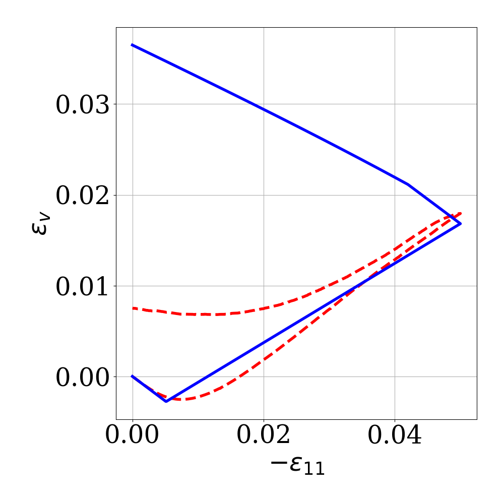
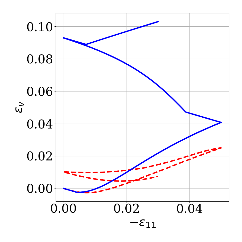
The statistics of the game scores played for the ”Calibration/Defense” by the protagonist and the ”Falsification/Attack” by the adversary during the DRL iterations are shown in Fig. 15. The AI agents only know the experimental decision tree and the rules of the two-player game without any prior knowledge on the strengths and weaknesses of the SANISAND model. The improvement of the protagonist’s policy is shown by the increase of the median of game scores, and also the narrowing of inter-quantile ranges. Some lower scores encountered during the later iterations of the DRL are due to random explorations of game strategies by the agent. Fig. 16 provides some example experiments selected by the protagonist for calibration data and Fig. 18 provides some example response curves associated to these experiments. Meanwhile, the adversary tries to attack the models calibrated by the protagonist using some experiments as shown in Fig. 17. Fig. 19 gives example response curves associated to these adversarial decision tree paths. These attacks inform and drive the protagonist to find more adequate calibration data via the score systems in this game.
In the end, the protagonist concludes that the model is accurate in modeling the mechanical behaviour of a single sample in TTC test with monotonic loading. In this case, the final value explored for is , which is slightly above the lower bound in the game score setting. Hence the decay coefficient in Eq. (10) is not activated and the protagonist score is equal to the calibration score. The adversary concludes that, when calibrated with this monotonic TTC data, the model is not accurate in predicting DTC, DTE, TTC experiments on other samples with unloading-reloading. Nevertheless, based on all the game episodes played during the DRL, the agents learn that the SANISAND model is capable of replicating the hardening-softening and contraction-dilation behavior of a densely compressed granular material. They also learn that SANISAND is more powerful than Drucker-Prager in replicating data from samples with different initial confinement, initial void ratio, test types, and unloading-reloading paths. The not perfect calibrations and forward predictions as shown in Fig. 18 and Fig. 19 may be due to the choice of calibration procedures, or because the formulations of SANISAND are designed based on the real sand behaviour, but our data comes from DEM numerical samples.


Defense Game Score: 0.162

Defense Game Score: 0.626

Defense Game Score: 0.687

Defense Game Score: 0.912
Attack Game Score: 0.206
Attack Game Score: 0.323

Attack Game Score: 0.295
Attack Game Score: -0.290

Defense Game Score: 0.162

Defense Game Score: 0.626

Defense Game Score: 0.687

Defense Game Score: 0.912

Defense Game Score: 0.162

Defense Game Score: 0.626

Defense Game Score: 0.687

Defense Game Score: 0.912
Attack Game Score: 0.206
Attack Game Score: 0.323
Attack Game Score: 0.295
Attack Game Score: -0.290
Attack Game Score: 0.206
Attack Game Score: 0.323
Attack Game Score: 0.295
Attack Game Score: -0.290
5.3 Experiment 3: Deep learning graph-based traction-separation model
The two-player non-cooperative game is played by DRL-based AI experimentalists for the data-driven traction-separation model. The neural network architectures and the calibration of the model are detailed in Section B.3. The game settings are for the protagonist and for the adversary, , . Hence the combination number of the selected experimental decision tree paths in this example is about . The hyperparameters for the DRL algorithm are , , , , , , , . The policy/value networks are identical to the ones used in the previous examples. In this example, since the number of the possible game configurations is enormous, we constrain the policy of the protagonist to play only the winning games (those who have got their rewards ) in 1/5 of the 40 game episodes in each training iteration and in the last iteration of ”competitive gameplays”. Also, we manually pre-select 10 experiments that have two loading cycles and regard them as the ”shared” test data. They need to be predicted by all calibrated traction-separation models, along with the test data selected by the adversary, in order to help explore in Eq. (10). These methods are applied in addition to the general reinforcement learning framework in Section 4 to enhance the convergence of the agents’ gameplay strategies.
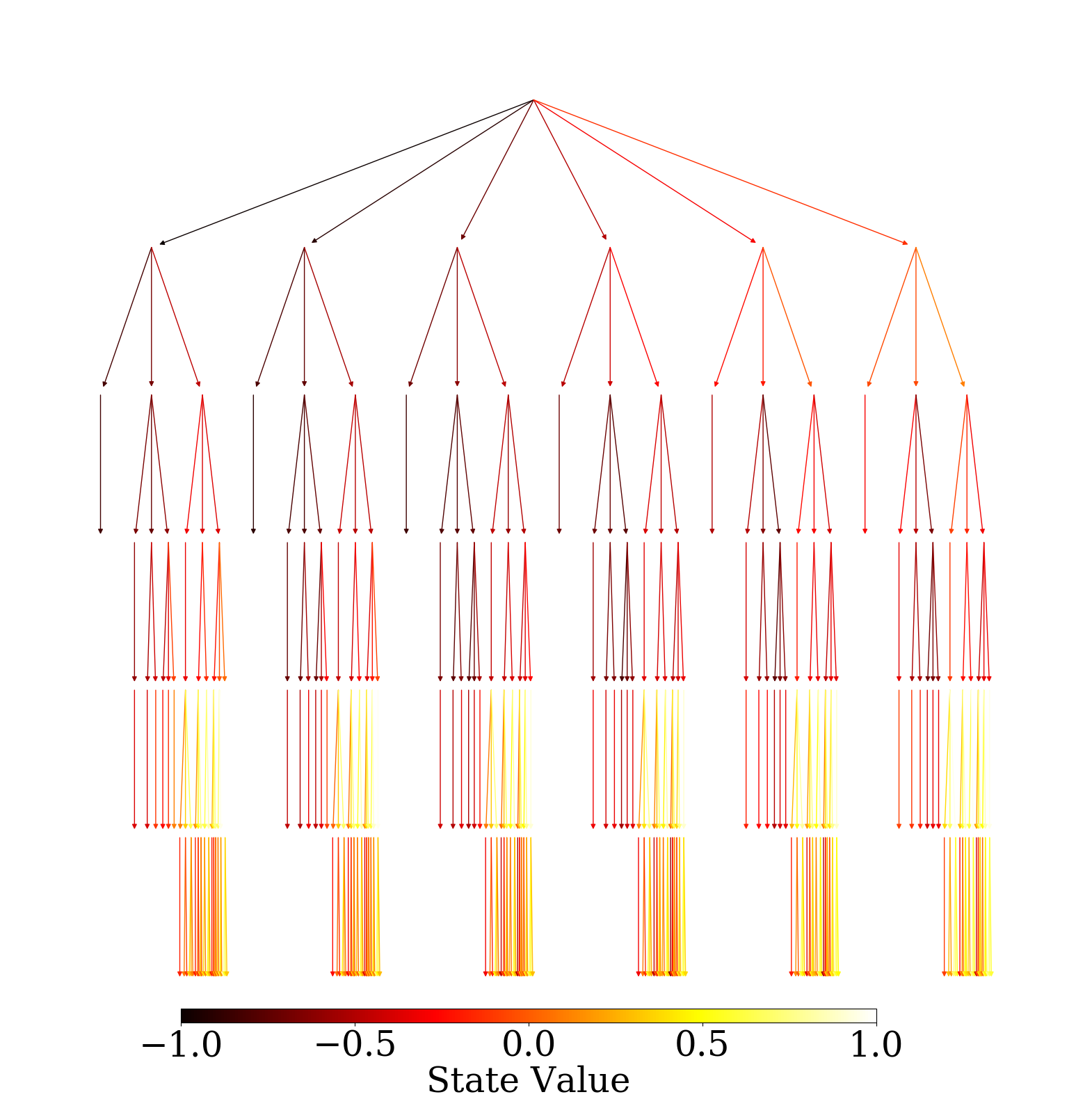
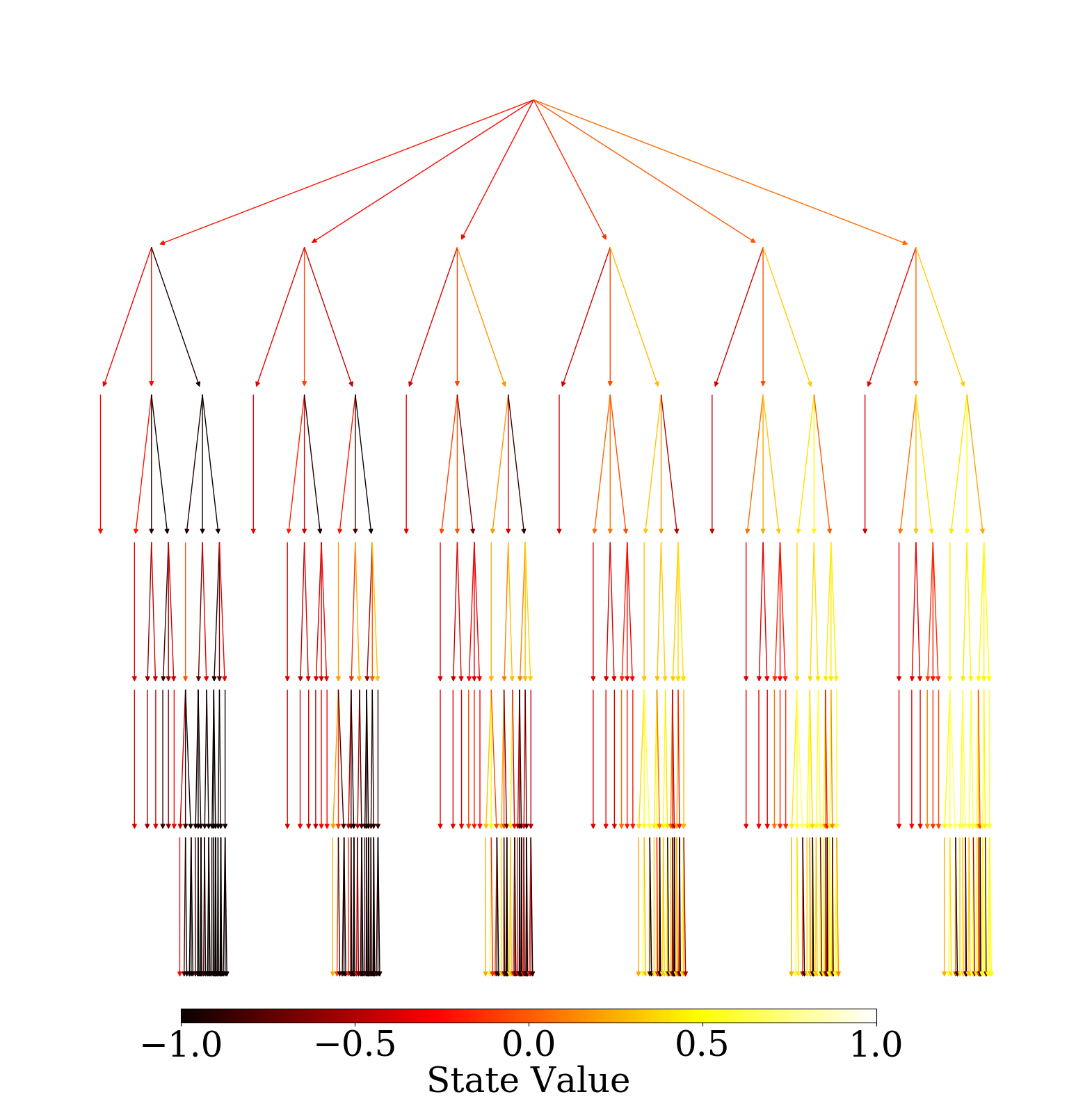
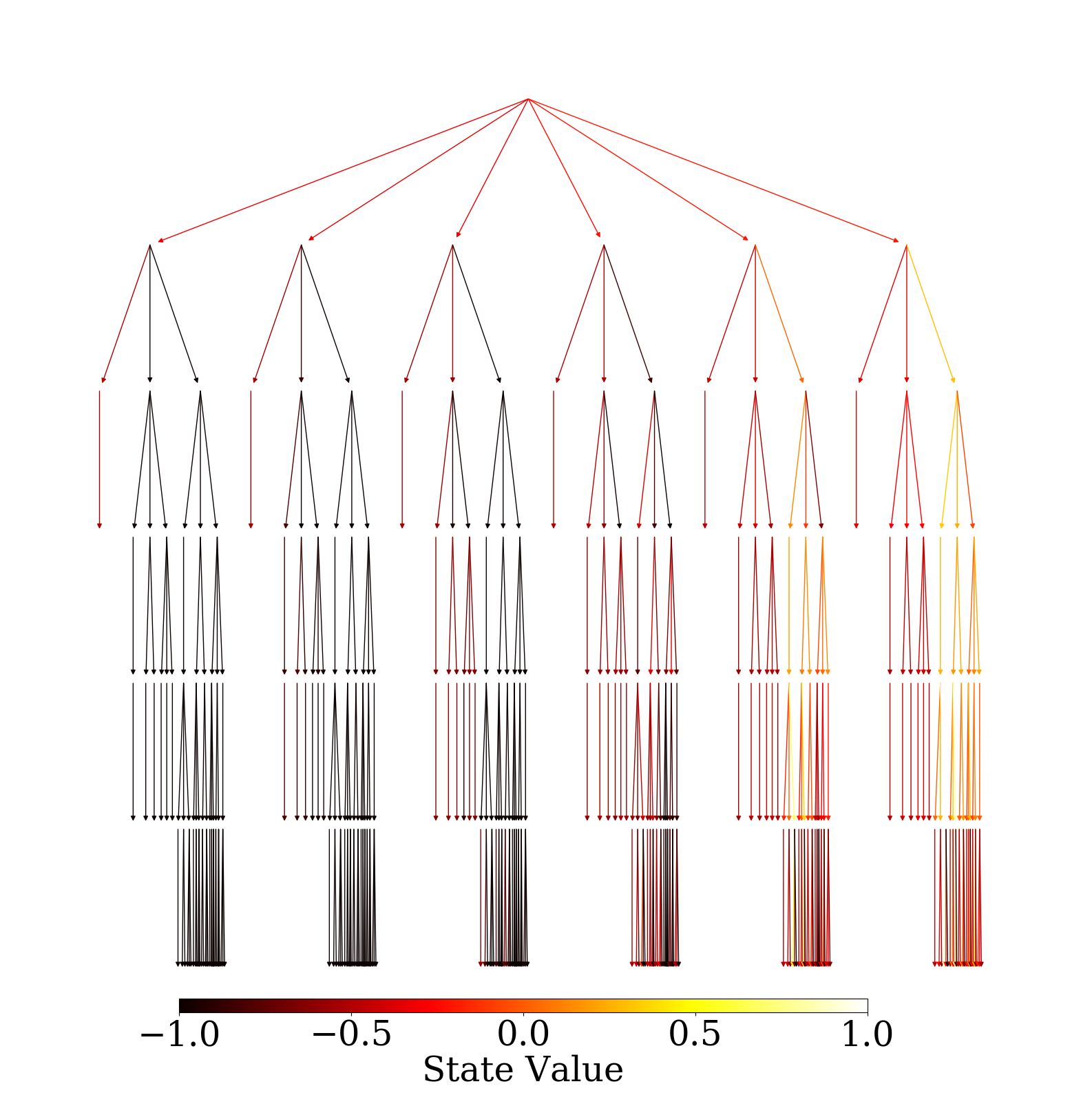
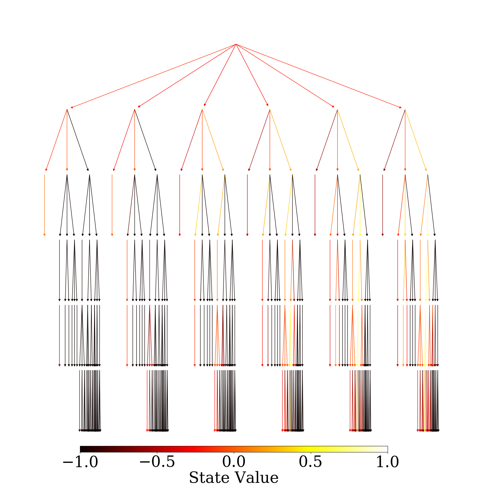
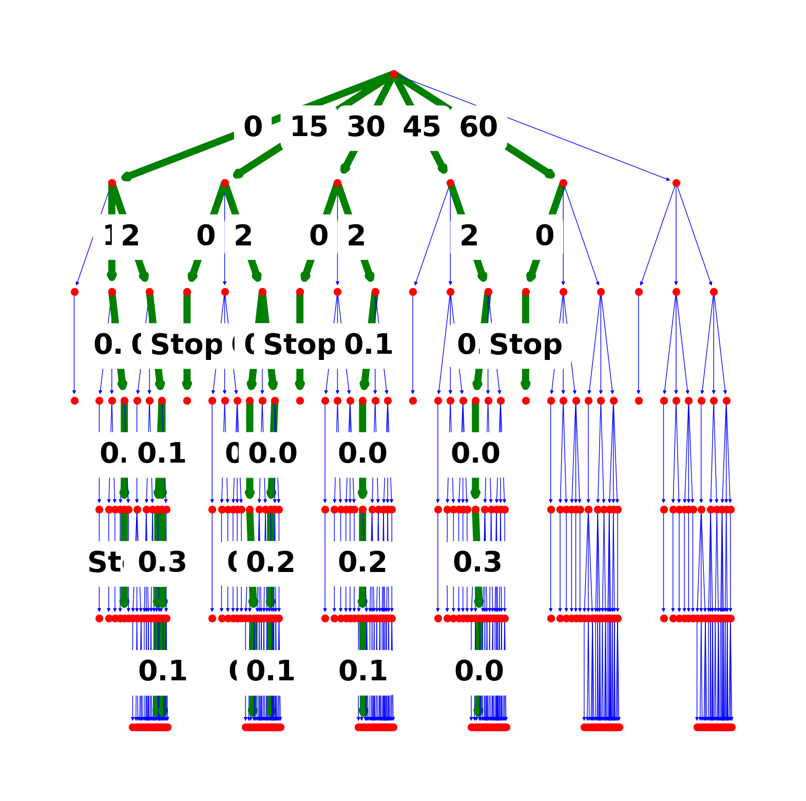
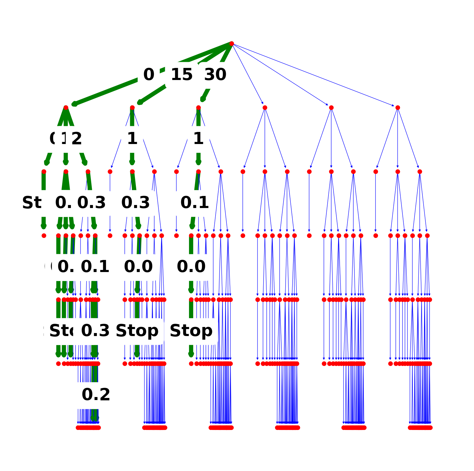
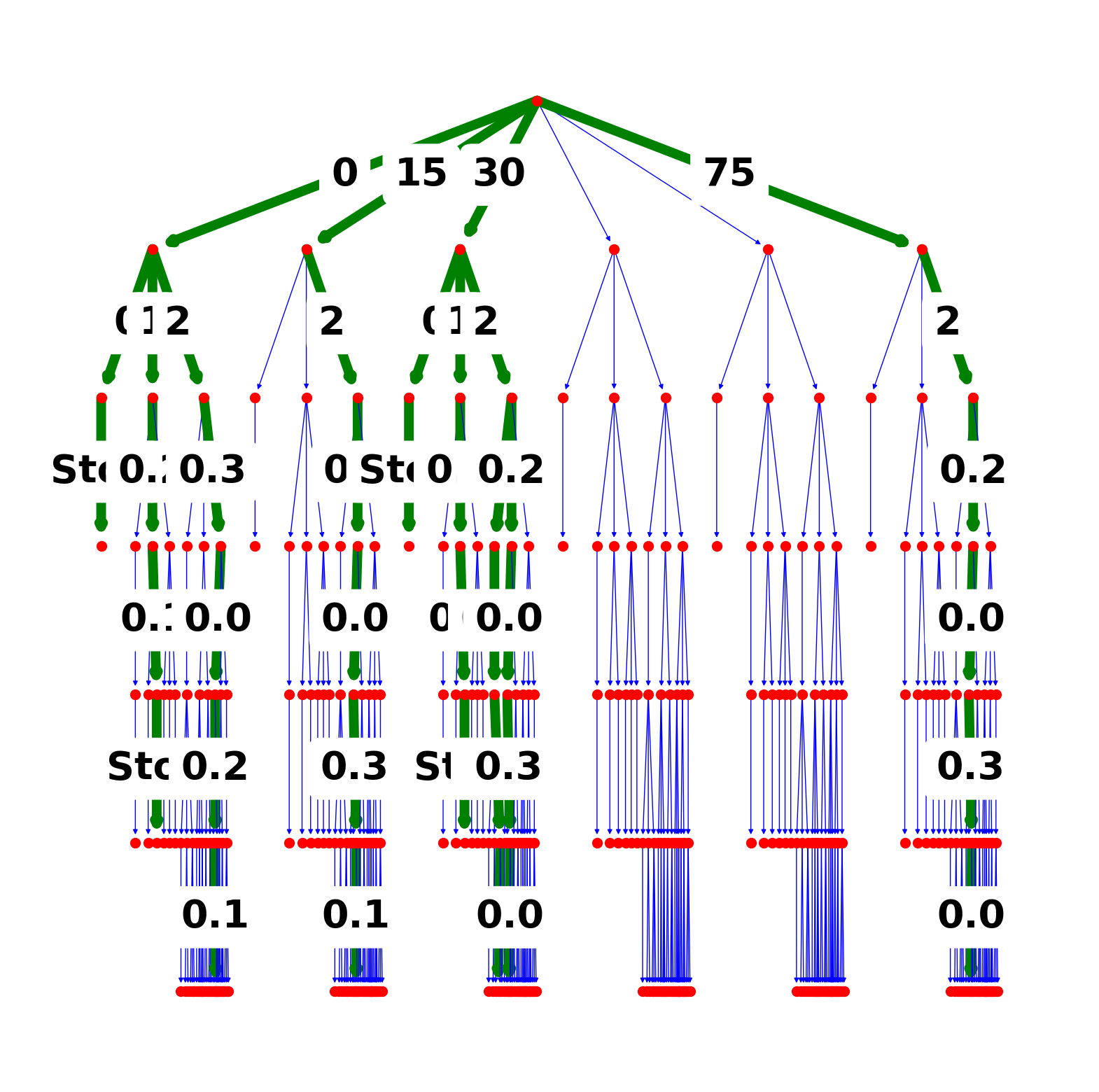
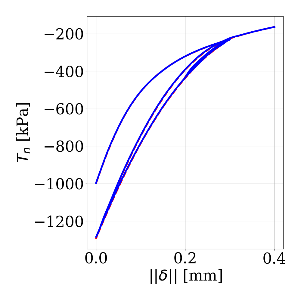
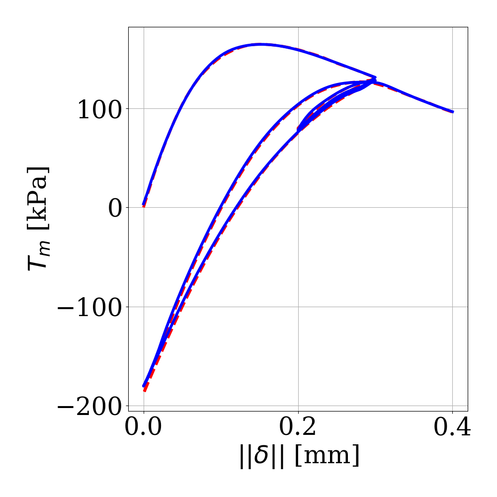
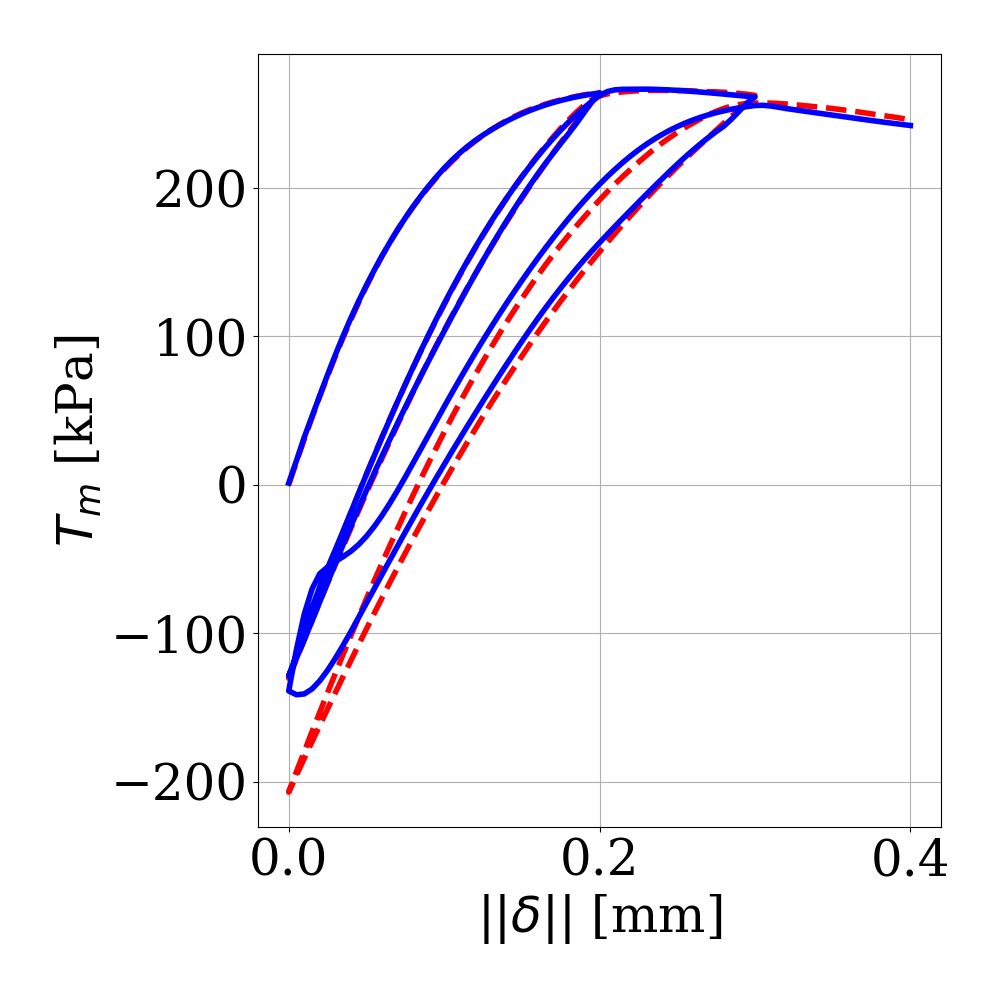
The statistics of the game scores played for the ”Calibration/Defense” by the protagonist and the ”Falsification/Attack” by the adversary during the DRL iterations are shown in Fig. 20. The improvement of the protagonist’s policy is shown by the increase of the median of game scores. Fig. 21 provides some examples of experiments selected by the protagonist for calibration data. The protagonist progressively develops the intelligence to select experiments from multiple displacement jump angles and multiple loading cycles, instead of concentrating on selections only cover very few angles and monotonic loading. This is consistent with intuitions from human experts, but is automatically discovered by the AI. We further include some examples of estimated Q-values of the experimental decision tree (Fig. 22) by the protagonist to illustrate how the agent is learning during the DRL. We record the agent’s policy/value network trained after each iteration of the DRL. Each checkpoint is used to predict the Q-value of each possible state in the experimental decision tree. The figure presents the expectations from the protagonist, before choosing any experiments, on how beneficial if an experiment is included in the calibration data. The evolution of the colors illustrates the progressively improved Q-value estimations learned from the game episodes and their rewards collected during the DRL.


Defense Game Score: -0.992

Defense Game Score: -0.331

Defense Game Score: 0.269

Defense Game Score: 0.879
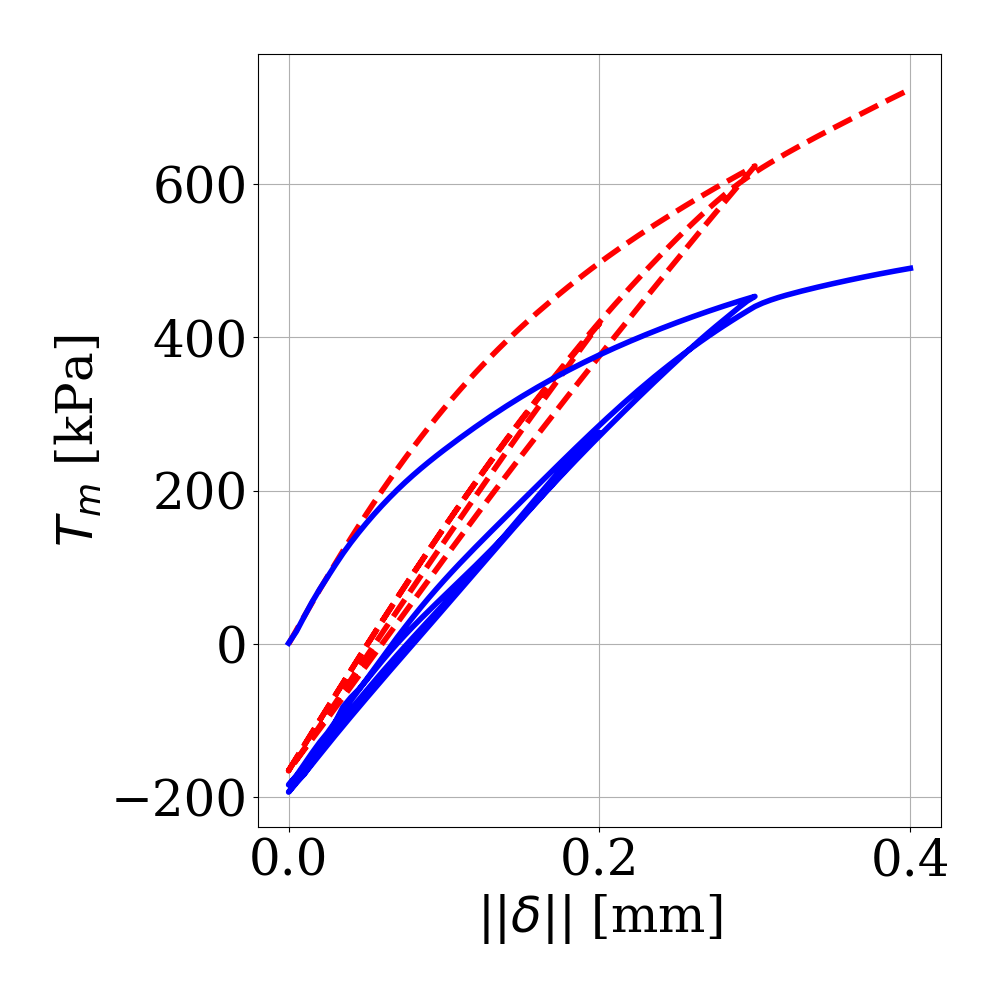
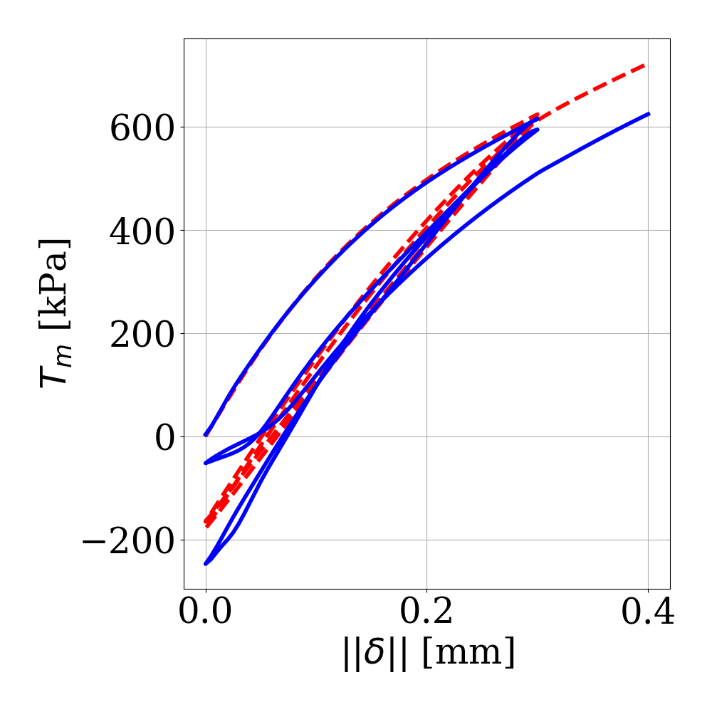
Meanwhile, the adversary’s scores also tend to increase as opposed to the previous examples. This could be attributed to the fact that the increasingly well-trained model by the protagonist using more effective calibration data, hence the corresponding prediction accuracy on unseen testing data also increases. Nevertheless, the adversarial game objective keeps driving the adversary to explore the model’s weakest performance. This feedback loop plays an important role in forcing the protagonist to find more adequate calibration data to make the model more resilient to attacks orchestrated by the adversary agent, based on improved skills learned from previous walks on the decision tree. Some example experiments selected by the adversary for testing data along the DRL are provided in Fig. 23.
Attack Game Score: -0.085
Attack Game Score: -0.127
Attack Game Score: 0.540
Attack Game Score: 0.443
In this example, we observe a slow convergence of the game policies as shown by the score distributions in Fig. 20. We attribute these difficulties to the following factors.
-
1.
The game dimension of this example is where 228 is the total number of leaves in the decision tree (cf. Section 2.2) and 10 is the maximum number of paths chosen by the agent (), even when the agents try to follow the best policy learned from previous gameplay experiences, a slight deviation from this policy due to the freedom of ”exploration” may lead to significant deterioration on the game performance.
-
2.
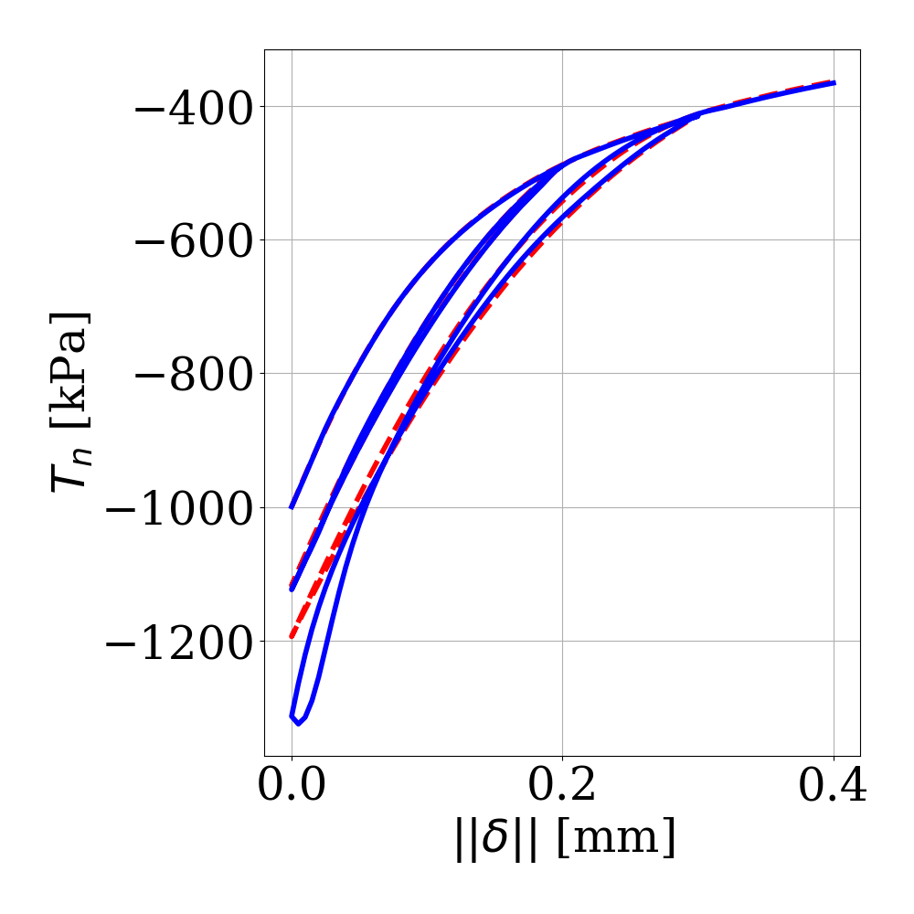
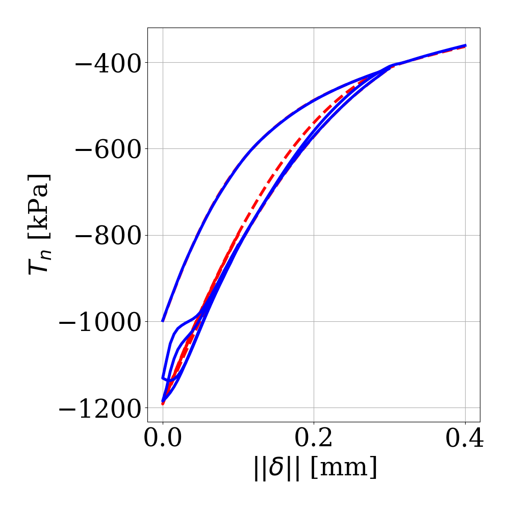
The ANN-based traction-separation model is highly adaptive to the calibration data. Neural networks can be trained very accurately to a broad range of calibration data, without changing its architecture. The handcrafted models from experts, however, are developed from fixed theory and have fixed mathematical expressions. They are not flexible to significant changes in calibration data. This can be seen from the example response curves in Fig. 24. Because the calibration scores are uniformly high, the performance of the protagonist can not be judged solely based on the calibration accuracy.
-
3.
The performance of the protagonist mainly depends on the prediction accuracy on unseen testing data. This accuracy and hence the score the protagonist received is nevertheless depends on the data generated from experiments designed by the adversary.
At the early stage of the game, the adversary is learning from scratch without any human knowledge provided. As a result, the Q table of the adversary may not be accurate enough to find the best way to attack the trained model properly in the first DRL iterations. Some gameplays from the protagonist may yield an apparently high reward, because the adversary may design experiments very similar to that of the protagonist used for calibration. For example, the protagonist may only train the model with monotonic loading and few loading angles, whereas the adversary also test the model on monotonic loadings. The reward in this case is apparently to be high. However, since there has not been enough exploration done, the Q tables for both agents are not sufficiently accurate to yield a score that carries credibility to judge the performance of the unexplored loading paths characterized by a subset of possible walks in the decision tree.

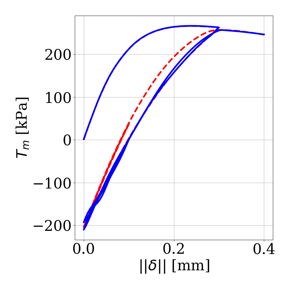
Defense Game Score: -0.992
Defense Game Score: -0.331

Defense Game Score: 0.269

Defense Game Score: 0.879

Defense Game Score: -0.992
Defense Game Score: -0.331
Defense Game Score: 0.269

Defense Game Score: 0.879
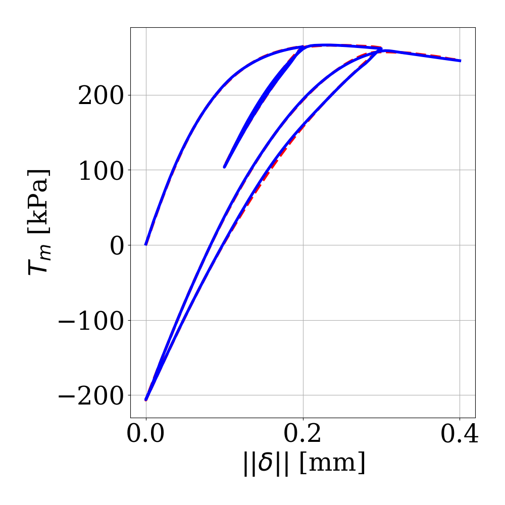
At the late stage of the game (Iteration 10), the DRL is capable of improving the blind prediction capability of the data-driven models, as shown in Fig. 25. This result is attributed to the fact that the Q table of the protagonist has been sufficiently improved such that it is able to design experiments that calibrate the model much better. While adversary agent that launch the adversarial attacks are given the same opportunities to improve its own Q table and therefore the policy decision skills, its action no longer exposes any particularly severe weakness of the model. such attributes are encouraging sign that shows the the machine learning model may provide efficiently robust predictions on unseen data.
Attack Game Score: -0.085
Attack Game Score: -0.127
Attack Game Score: 0.540
Attack Game Score: 0.443
Attack Game Score: -0.085
Attack Game Score: -0.127
Attack Game Score: 0.540
Attack Game Score: 0.443
More importantly, these three numerical experiments show that the the competition between the two agents is helpful to improve the robustness of the collective performance of both agents. This finding is consistent with previous efforts on the validation and blind predictions of material models such as the Sandia Fracture Challenges (Boyce et al., 2014, 2016) and the VELAS project (Arulanandan and Scott, 1993; Popescu and Prevost, 1995).
6 Conclusion and future perspectives
We introduce a multi-agent non-cooperative meta-modeling game in which the generation of calibration/validation data and the adversary testing data aided to falsify the model are handled by two competing artificial intelligence experimentalist agents. Mimicking the competition between a pair of protagonist and adversary in order to calibrate/validate and falsify a constitutive model for a path-dependent process, these two AI agents interact with each other sequentially and exchange information until both agents reach their own objectives and further actions do not gain better individual rewards. The winning strategies of the non-cooperative game are efficiently searched by the deep reinforcement learning (DRL) technique. The wide-applicability and efficiency of our approach have been shown through two elasto-plasticity models and a data-driven traction-separation model, with the number of possible game configurations as enormous as and , respectively. To the best knowledge of the authors, this is the first time the strategies of experimentalists who provide data to validate/falsify a history-dependent model are formulated in a non-cooperative decision-making game. Both agents are able to continuously improved their knowledge of the constitutive law using experimental data generated by each others in a competitive DRL framework (Silver et al., 2017b, a) and established the Nash equilibria strategies that tell us the quality of the models in the applications represented in the decision trees. Such innovations are necessary keys to develop powerful AI assistants that take over large amounts of trial-and-error burdens from human researchers for material modeling and knowledge discoveries with decision trees that are too deep to explore manually. More importantly, the competitive nature enables us to not only find the optimal setup of a constitutive laws, but also find out the weakness of the models in an unbiased third-party manner.
Further improvements and extensions can be made regarding the following aspects of our current framework. (1) Experimental data from real-world granular materials, instead of DEM samples, can be used if the AI agents’ decision trees are connected with laboratory instruments. (2) The rewards of the game strategies and hence the conclusions drawn from the game are sensitive to the game settings and the score systems (objective functions), e.g., the hyperparameters , , , . These game designs need to be tuned by human experts in order to appropriately investigate the strengths and weaknesses of the model. (3) They also depend on the calibration procedures, especially the elasto-plasticity models from human experts in which the material parameters have specific meanings and require initial guesses and bounds. The neural network models, on the other hand, can adapt to a wide range of material behaviour and calibrate well, but with material parameters difficult to interpret.
7 Acknowledgments
The work of KW and WCS is supported by National Science Foundation under grants contracts CMMI-1846875 and CMMI-1940203, the Earth Materials and Processes program from the US Army Research Office under grant contract W911NF-18-2-0306, the Dynamic Materials and Interactions Program from the Air Force Office of Scientific Research under grant contract FA9550-17-1-0169 and FA9550-19-1-0318, as well as the Columbia SEAS Interdisciplinary Research Seed Grant. The work of QD is supported in part by NSF CCF-1704833, DMS-1719699, DMR-1534910, and ARO MURI W911NF-15-1-0562. These supports are gratefully acknowledged. The views and conclusions contained in this document are those of the authors, and should not be interpreted as representing the official policies, either expressed or implied, of the sponsors, including the Army Research Laboratory or the U.S. Government. The U.S. Government is authorized to reproduce and distribute reprints for Government purposes notwithstanding any copyright notation herein.
Appendix A Preparation and experiments of DEM samples
The data for calibration and evaluation of the prediction accuracy of the constitutive models are generated by numerical simulations on representative volume elements (RVEs) of densely-packed spherical DEM particles. The open-source discrete element simulation software YADE for DEM is used by the AI experimentalist agents to generate data, including the homogenized stress and strain measures and the geometrical attributes such as porosity, coordination number and fabric tensor (Šmilauer et al., 2010).
The RVEs for AI-guided experimentation on bulk granular materials (Section 2.1) consist of discrete element particles having radii between mm with a uniform distribution. The Cundall’s elastic-frictional contact model ((Cundall and Strack, 1979)) is used for the inter-particle constitutive law. The material parameters are: interparticle elastic modulus GPa, ratio between shear and normal stiffness , frictional angle , density , Cundall damping coefficient . Firstly, a random loose packing enclosed in a parallelepiped of edge size mm is generated. The sample is then isotropically compressed to = -300 kPa. = 0.60 is approximated using a fictitious frictional angle of 0.05 rad, whereas = 0.55 is approximated using a frictional angle of 0.01 rad. These samples are then isotropically compressed to higher confinements = -400 kPa and = -500 kPa. The generated RVE samples for the AI experimentalists to choose are presented in Table 4. The ’DTC’, ’DTE’, ’TTC’ tests are conducted quasi-statically using the YADE engine ”PeriTriaxController”, and data are recorded at every strain increment of 1e-4.
| Sample No. | ’Sample ’ | ’Sample ’ | ||
| 1 | ’300kPa’ | ’0.60’ | -300 kPa | 0.5955 |
| 2 | ’300kPa’ | ’0.55’ | -300 kPa | 0.5554 |
| 3 | ’400kPa’ | ’0.60’ | -400 kPa | 0.5936 |
| 4 | ’400kPa’ | ’0.55’ | -400 kPa | 0.5538 |
| 5 | ’500kPa’ | ’0.60’ | -500 kPa | 0.5917 |
| 6 | ’500kPa’ | ’0.55’ | -500 kPa | 0.5521 |
The RVEs for AI-guided experimentation on granular interfaces (Section 2.2) consist of discrete element particles having radii between mm with a uniform distribution. The Cundall’s elastic-frictional contact model is used. The material parameters are identical to those of the bulk RVEs. The sample with initially random loose packing is isotropically compressed to = -1 MPa using a fictitious frictional angle of 0.01 rad. Hence the initial traction is -1 MPa in the normal direction and 0 MPa in the tangential direction. The width between the upper and lower surfaces of the sample is 20 mm. The mixed-mode shear tests with different loading paths are conducted quasi-statically, and data are recorded at every displacement jump increment of 0.005 mm.
Appendix B Material Models in Numerical Examples
B.1 Drucker–Prager elasto-plasticity model (Section 5.1)
The model adopts a linear elasticity law with the elastic stiffness tensor
| (14) |
where is the elastic bulk modulus and is the elastic shear modulus.
| (15) |
where is the reference shear modulus and is the Poisson ratio.
The yield surface has the form , where , , . The potential surface has the form . and evolve according to
| (16) |
where , , , and are material parameters to calibrate. is the accumulated plastic strain.
The calibration using the nonlinear least-squares solver ”NL2SOL” in Dakota software (Adams et al., 2014) requires initial guesses, upper and lower bounds of each parameter. They are given in Table 5. The elasticity parameters and are calibrated using the first three data points of each calibration experiment. They are fixed in the later calibration of plasticity parameters , , , , . The target features for calibration objectives and accuracy evaluations include data of the pressure , the deviatoric stress , and the volumetric strain .
| Parameter | Initial Guess | Lower Bound | Upper Bound |
|---|---|---|---|
| 6e4 kPa | 4e4 kPa | 8e4 kPa | |
| 0.25 | 0.1 | 0.4 | |
| 1.0 | 0.5 | 1.5 | |
| 2e4 | 1e2 | 6e4 | |
| 1e-5 1/Pa | 5e-6 1/Pa | 5e-5 1/Pa | |
| 60.0 | 20.0 | 200.0 | |
| 0.5 | 0.2 | 0.8 |
B.2 SANISAND elasto-plasticity model (Section 5.2)
The model is expressed in geomechanics sign convention as in the original paper. The model adopts the nonlinear elasticity with dependence on the mean pressure and the void ratio ,
| (17) |
where and are material parameters, = 100 kPa is the atmospheric pressure.
The yield surface has the shape of a small cone
| (18) |
where we fix to be 0.01.
The back stress-ratio tensor evolves according to
| (19) |
where is the rate of the plastic multiplier, and
| (20) |
where , , , , , , , are material parameters.
The plastic flow direction is defined as
| (21) |
where , , , are additional material parameters.
The initial guesses, upper and lower bounds of the above parameters for Dakota’s ”NL2SOL” calibration are given in Table 6. The calibration procedure is identical to that of Drucker–Prager model.
| Parameter | Initial Guess | Lower Bound | Upper Bound |
|---|---|---|---|
| 1e4 kPa | 5e3 kPa | 2e4 kPa | |
| 0.25 | 0.1 | 0.4 | |
| 0.75 | 0.5 | 1.0 | |
| 0.9 | 0.7 | 1.0 | |
| 0.8 | 0.7 | 0.9 | |
| 0.0025 | 0.0001 | 0.005 | |
| 1.0 | 0.8 | 1.2 | |
| 3.0 | 1.0 | 5.0 | |
| 0.5 | 0.01 | 1.0 | |
| 1.0 | 0.5 | 1.5 | |
| 30.0 | 10.0 | 50.0 | |
| 1.0 | 0.5 | 1.5 | |
| 600.0 | 400.0 | 800.0 | |
| 2.5 | 1.0 | 5.0 |
B.3 Data-driven traction-separation model (Section 5.3)
Data-driven traction-separation models use artificial neural networks (ANNs) as universal function approximators to continuous functions of various complexity on compact subsets of (Universal approximation theorem, (Hornik et al., 1989)). Moreover, a special type of ANNs, recurrent neural networks (RNN, e.g., long short-term memory (LSTM) (Hochreiter and Schmidhuber, 1997), gated recurrent units (GRU) (Cho et al., 2014; Chollet et al., 2015)), can capture the functions of a time series of inputs, which is appropriate for replicating the path-dependent material behaviors in granular interfaces. The data-driven model in the example firstly uses the histories of normal, tangential, accumulated norm, and maximum experienced norm of the displacement jumps through a RNN to predict the current normal and tangential fabrics of the interface. Then these displacement jump and fabric features are input together into a second RNN to predict the current normal and tangential traction across the interface. The parameters in each RNN are calibrated with training data of the corresponding input and output features using the backpropagation. Each RNN consists of two hidden layers with 32 GRU neurons in each layer, and the output layer is a dense layer with linear activation function. All input and output data are pre-processed by standard scaling using mean values and standard deviations (Pedregosa et al., 2011). Each input feature contains its current value and 4 history values prior to the current loading step. Each RNN is trained for 1000 epochs using the Adam optimization algorithm (Kingma and Ba, 2014), with a batch size of 128.
References
- Abadi et al. [2015] Martín Abadi, Ashish Agarwal, Paul Barham, Eugene Brevdo, Zhifeng Chen, Craig Citro, Greg S. Corrado, Andy Davis, Jeffrey Dean, Matthieu Devin, Sanjay Ghemawat, Ian Goodfellow, Andrew Harp, Geoffrey Irving, Michael Isard, Yangqing Jia, Rafal Jozefowicz, Lukasz Kaiser, Manjunath Kudlur, Josh Levenberg, Dandelion Mané, Rajat Monga, Sherry Moore, Derek Murray, Chris Olah, Mike Schuster, Jonathon Shlens, Benoit Steiner, Ilya Sutskever, Kunal Talwar, Paul Tucker, Vincent Vanhoucke, Vijay Vasudevan, Fernanda Viégas, Oriol Vinyals, Pete Warden, Martin Wattenberg, Martin Wicke, Yuan Yu, and Xiaoqiang Zheng. TensorFlow: Large-scale machine learning on heterogeneous systems, 2015. URL https://www.tensorflow.org/. Software available from tensorflow.org.
- Adams et al. [2014] Brian M Adams, WJ Bohnhoff, KR Dalbey, JP Eddy, MS Eldred, DM Gay, K Haskell, Patricia D Hough, and Laura P Swiler. Dakota, a multilevel parallel object-oriented framework for design optimization, parameter estimation, uncertainty quantification, and sensitivity analysis: Version 6.10 user’s manual. Sandia National Laboratories, Tech. Rep. SAND2014-4633, 2014.
- Arulanandan and Scott [1993] K Arulanandan and RF Scott. Project velacs—control test results. Journal of geotechnical engineering, 119(8):1276–1292, 1993.
- Bang-Jensen and Gutin [2008] Jørgen Bang-Jensen and Gregory Z Gutin. Digraphs: theory, algorithms and applications. Springer Science & Business Media, 2008.
- Berthelot et al. [2019] David Berthelot, Nicholas Carlini, Ian Goodfellow, Nicolas Papernot, Avital Oliver, and Colin A Raffel. Mixmatch: A holistic approach to semi-supervised learning. In Advances in Neural Information Processing Systems, pages 5050–5060, 2019.
- Bessa et al. [2017] MA Bessa, R Bostanabad, Zeliang Liu, A Hu, Daniel W Apley, C Brinson, Wei Chen, and Wing Kam Liu. A framework for data-driven analysis of materials under uncertainty: Countering the curse of dimensionality. Computer Methods in Applied Mechanics and Engineering, 320:633–667, 2017.
- Bonabeau [2002] Eric Bonabeau. Agent-based modeling: Methods and techniques for simulating human systems. Proceedings of the National Academy of Sciences, 99(suppl 3):7280–7287, 2002.
- Borja [2013] Ronaldo I Borja. Plasticity: modeling & computation. Springer Science & Business Media, 2013.
- Boyce et al. [2016] BL Boyce, SLB Kramer, TR Bosiljevac, E Corona, JA Moore, K Elkhodary, CHM Simha, BW Williams, AR Cerrone, A Nonn, et al. The second sandia fracture challenge: predictions of ductile failure under quasi-static and moderate-rate dynamic loading. International Journal of Fracture, 198(1-2):5–100, 2016.
- Boyce et al. [2014] Brad L Boyce, Sharlotte LB Kramer, H Eliot Fang, Theresa E Cordova, Michael K Neilsen, K Dion, Amy K Kaczmarowski, Erin Karasz, Liang Xue, Andrew J Gross, et al. The sandia fracture challenge: blind round robin predictions of ductile tearing. International Journal of Fracture, 186(1-2):5–68, 2014.
- Bryant and Sun [2018] Eric C Bryant and WaiChing Sun. A mixed-mode phase field fracture model in anisotropic rocks with consistent kinematics. Computer Methods in Applied Mechanics and Engineering, 342:561–584, 2018.
- Cho et al. [2014] Kyunghyun Cho, Bart Van Merriënboer, Caglar Gulcehre, Dzmitry Bahdanau, Fethi Bougares, Holger Schwenk, and Yoshua Bengio. Learning phrase representations using rnn encoder-decoder for statistical machine translation. arXiv preprint arXiv:1406.1078, 2014.
- Chollet et al. [2015] François Chollet et al. Keras. https://keras.io, 2015.
- Cundall and Strack [1979] Peter A Cundall and Otto DL Strack. A discrete numerical model for granular assemblies. geotechnique, 29(1):47–65, 1979.
- Dafalias [1984] Yannis F Dafalias. Modelling cyclic plasticity: simplicity versus sophistication. Mechanics of engineering materials, 153178, 1984.
- Dafalias and Manzari [2004] Yannis F Dafalias and Majid T Manzari. Simple plasticity sand model accounting for fabric change effects. Journal of Engineering mechanics, 130(6):622–634, 2004.
- De Bellis et al. [2017] Maria Laura De Bellis, Gabriele Della Vecchia, Michael Ortiz, and Anna Pandolfi. A multiscale model of distributed fracture and permeability in solids in all-round compression. Journal of the Mechanics and Physics of Solids, 104:12–31, 2017.
- Fang et al. [2017] Meng Fang, Yuan Li, and Trevor Cohn. Learning how to active learn: A deep reinforcement learning approach. arXiv preprint arXiv:1708.02383, 2017.
- Foerster et al. [2016] Jakob Foerster, Ioannis Alexandros Assael, Nando de Freitas, and Shimon Whiteson. Learning to communicate with deep multi-agent reinforcement learning. In Advances in Neural Information Processing Systems, pages 2137–2145, 2016.
- Graham et al. [1989] Ronald L Graham, Donald E Knuth, Oren Patashnik, and Stanley Liu. Concrete mathematics: a foundation for computer science. Computers in Physics, 3(5):106–107, 1989.
- Gupta et al. [2019] Ritesh Gupta, Simon Salager, Kun Wang, and WaiChing Sun. Open-source support toward validating and falsifying discrete mechanics models using synthetic granular materials—part i: Experimental tests with particles manufactured by a 3d printer. Acta Geotechnica, 14(4):923–937, 2019.
- He and Chen [2019] Qizhi He and Jiun-Shyan Chen. A physics-constrained data-driven approach based on locally convex reconstruction for noisy database. arXiv preprint arXiv:1907.12651, 2019.
- Heider et al. [2020] Yousef Heider, Kun Wang, and WaiChing Sun. So (3)-invariance of informed-graph-based deep neural network for anisotropic elastoplastic materials. Computer Methods in Applied Mechanics and Engineering, 363:112875, 2020.
- Hochreiter and Schmidhuber [1997] Sepp Hochreiter and Jürgen Schmidhuber. Long short-term memory. Neural computation, 9(8):1735–1780, 1997.
- Hornik et al. [1989] Kurt Hornik, Maxwell Stinchcombe, and Halbert White. Multilayer feedforward networks are universal approximators. Neural networks, 2(5):359–366, 1989.
- Kingma and Ba [2014] Diederik P Kingma and Jimmy Ba. Adam: A method for stochastic optimization. arXiv preprint arXiv:1412.6980, 2014.
- Kirchdoerfer and Ortiz [2016] Trenton Kirchdoerfer and Michael Ortiz. Data-driven computational mechanics. Computer Methods in Applied Mechanics and Engineering, 304:81–101, 2016.
- Kirchdoerfer and Ortiz [2017] Trenton Kirchdoerfer and Michael Ortiz. Data driven computing with noisy material data sets. Computer Methods in Applied Mechanics and Engineering, 326:622–641, 2017.
- Krause et al. [2005] Peter Krause, DP Boyle, and Frank Bäse. Comparison of different efficiency criteria for hydrological model assessment. Advances in geosciences, 5:89–97, 2005.
- Leibo et al. [2017] Joel Z Leibo, Vinicius Zambaldi, Marc Lanctot, Janusz Marecki, and Thore Graepel. Multi-agent reinforcement learning in sequential social dilemmas. In Proceedings of the 16th Conference on Autonomous Agents and MultiAgent Systems, pages 464–473. International Foundation for Autonomous Agents and Multiagent Systems, 2017.
- Littman [1994] Michael L Littman. Markov games as a framework for multi-agent reinforcement learning. In Machine learning proceedings 1994, pages 157–163. Elsevier, 1994.
- Liu et al. [2016] Yang Liu, WaiChing Sun, and Jacob Fish. Determining material parameters for critical state plasticity models based on multilevel extended digital database. Journal of Applied Mechanics, 83(1):011003, 2016.
- Mnih et al. [2013] Volodymyr Mnih, Koray Kavukcuoglu, David Silver, Alex Graves, Ioannis Antonoglou, Daan Wierstra, and Martin Riedmiller. Playing atari with deep reinforcement learning. arXiv preprint arXiv:1312.5602, 2013.
- Moritz et al. [2018] Philipp Moritz, Robert Nishihara, Stephanie Wang, Alexey Tumanov, Richard Liaw, Eric Liang, Melih Elibol, Zongheng Yang, William Paul, Michael I Jordan, et al. Ray: A distributed framework for emerging AI applications. In 13th USENIX Symposium on Operating Systems Design and Implementation (OSDI 18), pages 561–577, 2018.
- Na et al. [2019a] SeonHong Na, Eric C Bryant, and WaiChing Sun. A configurational force for adaptive re-meshing of gradient-enhanced poromechanics problems with history-dependent variables. Computer Methods in Applied Mechanics and Engineering, 357:112572, 2019a.
- Na et al. [2019b] SH Na, WC Sun, et al. A multi-phase-field/polycrystal plasticity for rock salt: micromorphic regularized grain-boundary slip. In 53rd US Rock Mechanics/Geomechanics Symposium. American Rock Mechanics Association, 2019b.
- Nash and Sutcliffe [1970] J Eamonn Nash and Jonh V Sutcliffe. River flow forecasting through conceptual models part i—a discussion of principles. Journal of hydrology, 10(3):282–290, 1970.
- Nash et al. [1950] John F Nash et al. Equilibrium points in n-person games. Proceedings of the national academy of sciences, 36(1):48–49, 1950.
- Olsson [2009] Fredrik Olsson. A literature survey of active machine learning in the context of natural language processing. 2009.
- Pack et al. [2014] Keunhwan Pack, Meng Luo, and Tomasz Wierzbicki. Sandia fracture challenge: blind prediction and full calibration to enhance fracture predictability. International Journal of Fracture, 186(1-2):155–175, 2014.
- Pedregosa et al. [2011] F. Pedregosa, G. Varoquaux, A. Gramfort, V. Michel, B. Thirion, O. Grisel, M. Blondel, P. Prettenhofer, R. Weiss, V. Dubourg, J. Vanderplas, A. Passos, D. Cournapeau, M. Brucher, M. Perrot, and E. Duchesnay. Scikit-learn: Machine learning in Python. Journal of Machine Learning Research, 12:2825–2830, 2011.
- Perolat et al. [2015] Julien Perolat, Bruno Scherrer, Bilal Piot, and Olivier Pietquin. Approximate dynamic programming for two-player zero-sum markov games. In Proceedings of the 32nd International Conference on Machine Learning, pages 1321–1329, 2015.
- Pinto et al. [2017] Lerrel Pinto, James Davidson, Rahul Sukthankar, and Abhinav Gupta. Robust adversarial reinforcement learning. In Proceedings of the 34th International Conference on Machine Learning-Volume 70, pages 2817–2826. JMLR. org, 2017.
- Popescu and Prevost [1995] Radu Popescu and Jean H Prevost. Comparison between velacs numerical ‘class a’predictions and centrifuge experimental soil test results. Soil Dynamics and Earthquake Engineering, 14(2):79–92, 1995.
- Rodriguez and Lade [2013] Nina M Rodriguez and Poul V Lade. True triaxial tests on cross-anisotropic deposits of fine nevada sand. International Journal of Geomechanics, 13(6):779–793, 2013.
- Sener and Savarese [2017] Ozan Sener and Silvio Savarese. Active learning for convolutional neural networks: A core-set approach. arXiv preprint arXiv:1708.00489, 2017.
- Settles [2009] Burr Settles. Active learning literature survey. Technical report, University of Wisconsin-Madison Department of Computer Sciences, 2009.
- Shen et al. [2017] Yanyao Shen, Hyokun Yun, Zachary C Lipton, Yakov Kronrod, and Animashree Anandkumar. Deep active learning for named entity recognition. arXiv preprint arXiv:1707.05928, 2017.
- Silver et al. [2017a] David Silver, Thomas Hubert, Julian Schrittwieser, Ioannis Antonoglou, Matthew Lai, Arthur Guez, Marc Lanctot, Laurent Sifre, Dharshan Kumaran, Thore Graepel, et al. Mastering chess and shogi by self-play with a general reinforcement learning algorithm. arXiv preprint arXiv:1712.01815, 2017a.
- Silver et al. [2017b] David Silver, Julian Schrittwieser, Karen Simonyan, Ioannis Antonoglou, Aja Huang, Arthur Guez, Thomas Hubert, Lucas Baker, Matthew Lai, Adrian Bolton, et al. Mastering the game of go without human knowledge. Nature, 550(7676):354–359, 2017b.
- Šmilauer et al. [2010] Václav Šmilauer, Emanuele Catalano, Bruno Chareyre, Sergei Dorofeenko, Jerome Duriez, Anton Gladky, Janek Kozicki, Chiara Modenese, Luc Scholtès, Luc Sibille, et al. Yade reference documentation. Yade Documentation, 474(1), 2010.
- Srivastava et al. [2014] Nitish Srivastava, Geoffrey Hinton, Alex Krizhevsky, Ilya Sutskever, and Ruslan Salakhutdinov. Dropout: a simple way to prevent neural networks from overfitting. The journal of machine learning research, 15(1):1929–1958, 2014.
- Tampuu et al. [2017] Ardi Tampuu, Tambet Matiisen, Dorian Kodelja, Ilya Kuzovkin, Kristjan Korjus, Juhan Aru, Jaan Aru, and Raul Vicente. Multiagent cooperation and competition with deep reinforcement learning. PloS one, 12(4):e0172395, 2017.
- Tan [1993] Ming Tan. Multi-agent reinforcement learning: Independent vs. cooperative agents. In Proceedings of the tenth international conference on machine learning, pages 330–337, 1993.
- Thacker et al. [2004] Ben H Thacker, Scott W Doebling, Francois M Hemez, Mark C Anderson, Jason E Pepin, and Edward A Rodriguez. Concepts of model verification and validation. Technical report, Los Alamos National Lab., 2004.
- Tu et al. [2009] Xuxin Tu, José E Andrade, and Qiushi Chen. Return mapping for nonsmooth and multiscale elastoplasticity. Computer Methods in Applied Mechanics and Engineering, 198(30-32):2286–2296, 2009.
- Verma et al. [2019] Vikas Verma, Alex Lamb, Juho Kannala, Yoshua Bengio, and David Lopez-Paz. Interpolation consistency training for semi-supervised learning. arXiv preprint arXiv:1903.03825, 2019.
- Vinyals et al. [2019] Oriol Vinyals, Igor Babuschkin, Wojciech M Czarnecki, Michaël Mathieu, Andrew Dudzik, Junyoung Chung, David H Choi, Richard Powell, Timo Ewalds, Petko Georgiev, et al. Grandmaster level in starcraft ii using multi-agent reinforcement learning. Nature, 575(7782):350–354, 2019.
- Wang and Sun [2018] Kun Wang and WaiChing Sun. A multiscale multi-permeability poroplasticity model linked by recursive homogenizations and deep learning. Computer Methods in Applied Mechanics and Engineering, 334:337–380, 2018.
- Wang and Sun [2019] Kun Wang and WaiChing Sun. Meta-modeling game for deriving theory-consistent, microstructure-based traction–separation laws via deep reinforcement learning. Computer Methods in Applied Mechanics and Engineering, 346:216–241, 2019.
- Wang et al. [2016] Kun Wang, Waiching Sun, Simon Salager, S Na, and Ghonwa Khaddour. Identifying material parameters for a micro-polar plasticity model via x-ray micro-ct images: lessons learned from the curve-fitting exercises. International Journal for Multiscale Computational Engineering, 14(4):389–413, 2016.
- Wang et al. [2019] Kun Wang, WaiChing Sun, and Qiang Du. A cooperative game for automated learning of elasto-plasticity knowledge graphs and models with ai-guided experimentation. Computational Mechanics, pages 1–33, 2019.
- West et al. [2001] Douglas Brent West et al. Introduction to graph theory, volume 2. Prentice hall Upper Saddle River, 2001.
- Wiering [2000] MA Wiering. Multi-agent reinforcement learning for traffic light control. In Machine Learning: Proceedings of the Seventeenth International Conference (ICML’2000), pages 1151–1158, 2000.
- Yang and Perdikaris [2019] Yibo Yang and Paris Perdikaris. Adversarial uncertainty quantification in physics-informed neural networks. Journal of Computational Physics, 394:136–152, 2019.
- Zhu and Bento [2017] Jia-Jie Zhu and José Bento. Generative adversarial active learning. arXiv preprint arXiv:1702.07956, 2017.
- Zhu [2005] Xiaojin Jerry Zhu. Semi-supervised learning literature survey. Technical report, University of Wisconsin-Madison Department of Computer Sciences, 2005.
- Zhu et al. [2019] Yinhao Zhu, Nicholas Zabaras, Phaedon-Stelios Koutsourelakis, and Paris Perdikaris. Physics-constrained deep learning for high-dimensional surrogate modeling and uncertainty quantification without labeled data. Journal of Computational Physics, 394:56–81, 2019.