R package SamplingStrata: new developments and extension to Spatial Sampling

Abstract

The R package SamplingStrata was developed in 2011 as an instrument to optimize the design of stratified samples. The optimization is performed by considering the stratification variables available in the sampling frame, and the precision constraints on target estimates of the survey (Ballin & Barcaroli, 2014). The genetic algorithm at the basis of the optimization step explores the universe of the possible alternative stratifications determining for each of them the best allocation, that is the one of minumum total size that allows to satisfy the precision constraints: the final optimal solution is the one that ensures the global minimum sample size. One fundamental requirement to make this approach feasible is the possibility to estimate the variability of target variables in generated strata; in general, as target variable values are not available in the frame, but only proxy ones, anticipated variance is calculated by modelling the relations between target and proxy variables. In case of spatial sampling, it is important to consider not only the total model variance, but also the co-variance derived by the spatial auto-correlation. The last release of SamplingStrata enables to consider both components of variance, thus allowing to harness spatial auto-correlation in order to obtain more efficient samples.

Keywords— stratified sampling, strata optimization, genetic algorithm, spatial sampling, best allocation

1 Introduction

The R package SamplingStrata (Barcaroli et al., 2020) is an instrument for the optimization of stratified sampling. It has been described in detail in Barcaroli (2014), Ballin & Barcaroli (2016) and Ballin & Barcaroli (2020a) . The first release of the R package SamplingStrata was made available on the CRAN in July 2011. At the time, the package was being used only internally in the Italian Institute of Statistics (Istat), in particular for agricultural surveys. Since then, as far as we know, SamplingStrata has been used in the New Zealand Statistical Institute, tested at Statistics Denmark and considered for evaluation at Statistics Canada. Eurostat used SamplingStrata for designing its 2018 LUCAS survey (Ballin et al., 2018). Bank of Italy, supported by Istat, adopted SamplingStrata to re-design its Survey on Households Income and Wealth. Also World Bank adopted SamplingStrata and embedded it in its SurveySolutions SamplingTools integrated application. Very recently, the NOAA Alaska Fisheries Science Center adopted SamplingStrata for its survey on fish populations in the Gulf of Alaska.

Figure 1 illustrates the relative importance among all packages in the CRAN: rank in terms of downloads is such that SamplingStrata comes before the 82% of the about 18,000 packages, despite its highly specific character.

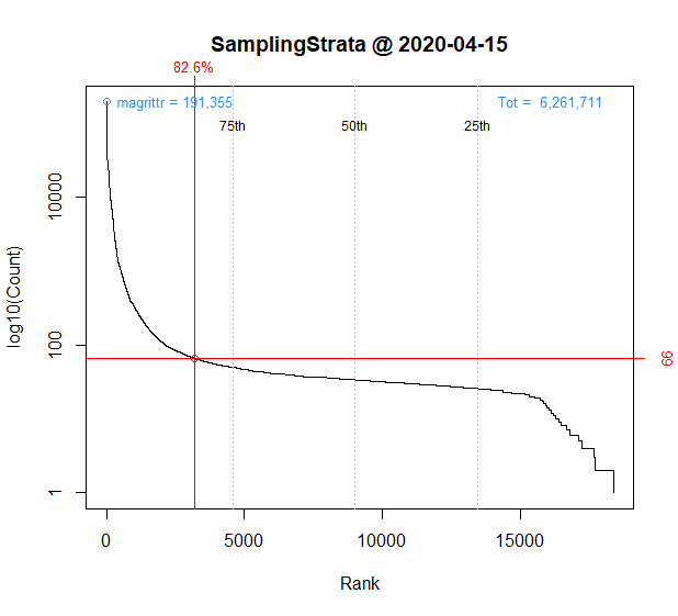
Figure 1: Rank of SamplingStrata in terms of downloads from the CRAN

This interest is also due to the improvements that in last two years have been produced by new developments aimed to

• increase the processing performance of the optimization step;

• extend the applicability of the instrument.

With regard to performance, in many occasions the processing time required to perform the optimization step in SamplingStrata has been a point of weakness of the package. Compared to the seconds taken by package stratification to perform the same task, the minutes (or even hours) required by SamplingStrata have been a relevant problem for users. The answers to this problem were:

1. the adoption of a variant of the Genetic Algorithm at the basis of function optimizeStrata, i.e. the Grouping Genetic Algorithm;

2. the development of a completely new optimization algorithm, which does not operate by aggregating atomic strata, but by randomly cutting the domain of each (continuous) stratification variable.

As for the applicability, the following extensions have been implemented in the package:

1. the possibility to model the relationships between auxiliary variables available in the frame and the variables of interest, in order to correctly estimate the variance of the latter (anticipated variance);

2. the opportunity to consider the geographical localization of the units in the frame and hence to take into account their spatial auto-correlation, in order to correctly determine the best stratification in spatial sampling.

The increasing availability of georeferenced or geocoded sampling frames makes this second point extremely important. For instance, in the Italian Statistical Institute this availability is guaranteed by the Registro Statistico di Base dei Luoghi, RSBL (Base Statistical Register of Places). We remind that RSBL offers different levels of geolocation of the statistical units: punctual (coordinates), irregular polygons (sections, municipalities, etc.), regular polygons (EU grids) accompanied by the corresponding geographic files necessary for determining spatial relations.

In order to extend the applicability of SamplingStrata to spatial sampling using the methodology suggested by de Gruijter et al. (2015), two additional functionalities have been implemented consisting in:

1. to extend the possibility to handle the anticipated variance to cases in which a Spatial Linear Model is applicable (full parametric approach);

2. to make available a different approach that requires as input for each point both prediction and prediction errors (non parametric approach).

In the parametric approach, the parameters of a Spatial Linear Model are explicitly supplied, while in the non parametric approach only the parameter related to the range of spatial correlation must be supplied. In both cases, geographical coordinates have to be supplied for each unit in the frame.

In order to ensure continuity with previous applications, the old optimization functions (as optimizeStrata and optimizeStrata2 remain in the package, but a new generic optimization function, namely optimStrata, has been made available, with a specific parameter, method, that indicates the type of algorithm that will be used in the optimization step:

1. method = "atomic" implies the use of the old algorithm implemented in optimizeStrata;

2. method = "continuous" implies the use of the algorithm applicable in case of all continuous stratification variables;

3. method = "spatial" implies the use of the new algorithm implementing the non parametric approach for spatial sampling.

This paper is structured as follows. In Section 2 a description of improvements in the optimization step is given, with some details on the adoption of the Genetic Grouping Algorithm to increase the performance of the already available optimization step, the development of the new function optimizeStrata2 covering the optimization step, and the handling of anticipated variance. In Section 3 the general approach followed to extend the applicability of the package to spatial sampling is illustrated. In Section 4.1 is reported an application of the non parametric approach to a widely used example (dataset meuse). Section 4.2 reports an application of both approaches to the case of optimization of the stratification of a frame where the selection units are Census Enumeration Areas. Finally, in Section 5 some conclusions are given, together with indications on future developments.

The R scripts together with data necessary to replicate the two case studies are available at the link https://github.com/barcaroli/R-scripts.

The version of SamplingStrata including developments here illustrated is downloadable from the link https://github.com/barcaroli/SamplingStrata.

2 Improvements in the optimization algorithms

The initial version of the SamplingStrata optimization function (optimizeStrata) (now optimStrata with method = "atomic") was based on the use of a plain Genetic Algorithm (GA). The starting point was the construction of the atomic stratification, obtained as the Cartesian product of the stratification variables, all rigorously categorical (if continuous, a discretization step was required). Every possible given stratification was obtained as an aggregation of atomic strata. In this setting, each stratification is represented by a vector of labels, whose length is equal to the number of atomic strata: atomic strata that share the same label in the vector are collapsed in an aggregate stratum. For each stratum (atomic or aggregate) mean and standard deviation of target variables are calculated by considering their values (or the values of related proxy variables) in the sampling frame. For each stratification, required sample size (and related cost) is calculated by applying the Bethel algorithm (Bethel, 1989), under given precision constraints on target estimates. In the GA approach, each vector representing a stratification is considered an (individual) in a (generation), and its (fitness) is measured by the associated sample cost. The usual GA operators (mutation) and (crossover) are applied in order to produce a new generation from the current one. After a given number of iterations, the best solution represents the stratification with the associated minimum sample cost, compliant with precision constraints.

2.1 Changes to GA operators selection and crossover

The optimization step previously described is formalized in Algorithm 1.

input : sampling frame, precision constraints, atomic strata

output : optimal stratification of the sampling frame

REM generate first population pop[1,];

for $j\leftarrow 1$ to $popSize$ do

       generate randomly a vector pop[1,j] of integers (from 1 to maxstrata);

       aggregate atomic strata using pop[1,j] vector;

       calculate sample.cost(pop[1,j]) applying Bethel algorithm on resulting aggregate strata;

       store pop[1,j] with min(sample.cost) as bestSolution;

      

end for

REM generate next populations pop[i,];

for $i\leftarrow 2$ to $iterations$ do

       apply selection and crossover operators to population pop[i-1,];

       generate individuals in pop[i,];

       apply mutation operator to pop[i,];

       for $j\leftarrow 1$ to $popSize$ do

             aggregate atomic strata using pop[i,j] vector;

             calculate sample.cost(pop[i,j]) applying Bethel algorithm on resulting aggregate strata;

             if sample.cost(pop[i,j] $<$ sample.cost(bestSolution) then bestSolution $\leftarrow$ pop[i,j];

            

       end for

      

end for

Algorithm 1 Function ’optimStrata’ algorithm (method = "atomic")

As previously mentioned, using the conventional GA operators the convergence towards the best solution can be exceedingly slow.

Following some of the indications contained in O’Luing et al. (2017) and O’Luing et al. (2019), two of the three GA operators were modified, i.e. selection and crossover, accordingly to the Grouping Genetic Algorithm (GGA) approach (the mutation operator remained unchanged). As for selection, instead of selecting parents for breeding completely at random, a probability of selection has been defined by means of a fitness function, in order to privilege most promising individuals. As for crossover, instead of mixing chromosomes in an undifferentiated way, groups of them in one parent (representing already aggregated strata) are attributed to the other parent when generating a child, preserving their composition.

The introduction of these innovations since release 1.2 allowed to substantially increase the performance of the optimization function.

2.2 New optimization algorithm

We recall that the version of optimization so far described is applicable only to categorical stratification variables: were they not categorical, they have to be discretized, obtaining categorical ordinal variables. A criticism of survey managers is that strata in the optimal solution are of difficult interpretation, as values of stratification variables in a given stratum in general are not contiguous. This problem is relevant when stratification variables are of the continuous type: as already said, they have to be discretized, and there is no warranty that in each resulting optimized stratum the values of this variables are contiguous, i.e. without "holes".

In order to overcome this problem, a new optimization algorithm, still making use of the Genetic Algorithm, has been implemented. This new version, first implemented in the function optimizeStrata2, now in optimStrata with method = "continuous", is applicable only when all the stratification variables are of the continuous type. Instead of building the atomic strata previously to the optimization step and proceeding to aggregate them, with this new function an individual in a population (a given stratification) is generated by randomly cutting the domains of definition of each stratification variable, and by producing the stratification by applying the Cartesian product to the so obtained discretized values. Then, the optimization proceeds as formalized in Algorithm 2. Under this new approach, the genoma of a solution is given by the sequence of cuts for the different stratification variables.

As a result, the obtained strata are "7-shaped" like the ones reproduced in Figure 2.

It can be seen that strata are characterized by given non overlapping intervals of values for each stratification variable.
Moreover, in many situations the convergence to the optimal solution can be much quicker with this new algorithm than with the previous one. The suggestion is to try both and analyze the different results in order to choose the best.

Figure 2: Example of 7-shaped strata obtained with continuous method

input : sampling frame, precision constraints

output : optimal stratification of the sampling frame

REM generate randomly first population pop[1,];

for $j\leftarrow 1$ to $popSize$ do

       for $k\leftarrow 1$ to $numVar$ do

             generate randomly n cuts (n = nStrata -1) in the definition domain of stratification variable k;

             concatenate the n cuts to the vector pop[1,j];

            

       end for

      generate strata using pop[1,j] vector;

       calculate sample.cost(pop[1,j]) applying Bethel algorithm on resulting aggregate strata;

       store pop[1,j] with min(sample.cost) as bestSolution;

      

end for

REM generate next populations pop[i,];

for $i\leftarrow 2$ to $iterations$ do

       apply selection and crossover operators to population pop[i-1,];

       generate individuals in pop[i,];

       apply mutation operator to pop[i,];

       for $j\leftarrow 1$ to $popSize$ do

             generate strata using pop[i,j] vector;

             calculate sample.cost(pop[i,j]) applying Bethel algorithm on resulting aggregate strata;

             if sample.cost(pop[i,j] $<$ sample.cost(bestSolution) then bestSolution $\leftarrow$ pop[i,j];

            

       end for

      

end for

Algorithm 2 Function ’optimStrata’ algorithm (method = "continuous")

2.3 Anticipated variance

When optimizing the stratification of a sampling frame, it is assumed that the values of the target variables Y’s are available for the generality of the units in the frame, or at least for a sample of them, by means of which it is possible to estimate means and standard deviations of Y’s in atomic strata. Of course, this assumption is seldom expected to hold. A much more common situation is the one where Y’s are proxy variables of the real target variables (named Z). In these cases, there is no guarantee that the final stratification and allocation can ensure the compliance to the set of precision constraints for the real target variables. The importance of considering anticipated variance has been clearly evidenced in Lisic et al. (2018).

In order to take into account this problem, and to limit the risk of overestimating the expected precision levels of the optimized solution, it is possible to carry out the optimization by considering, instead of the expected coefficients of variation related to proxy variables, the anticipated coefficients of variation (ACV) that depend on the model that is possible to fit on couples of real target variables and proxy ones.

In the current implementation, only models linking continuous variables can be considered. The definition and the use of these models is the same that has been implemented in the package stratification (Baillargeon & Rivest, 2014). In particular, the reference here is to two different models, the linear model with heteroscedasticity:

$Z=\beta Y+\epsilon$

where

$\epsilon\sim\ N(0,\sigma^{2}Y^{2\gamma})$

(in case $\gamma$ = 0 the model is homoscedastic)

and the loglinear model:

$Z=exp(\beta log(Y)+\epsilon)$

where

$\epsilon\sim\ N(0,\sigma^{2})$

In the case of the linear model the anticipated variance (AV) on a total is given by the following expression (Lisic et al., 2018):

$AV(\hat{T}_{j})=\sum_{h=1}^{H}(1-\dfrac{n_{h}}{N_{h}})\dfrac{N_{h}^{2}}{n_{h}}(\sum_{i=1}^{N_{h}}Y_{i,j}^{2\gamma}\sigma^{2}+\sum_{i=1}^{N_{h}}(y_{i}\beta_{j}-\bar{y}_{h}\beta_{j})^{2})$

Using a linear model, in case of presence of heteroscedasticity ($\gamma>0$) in residuals distribution, a crucial point is in correctly quantifying it. The problem of how to estimate a measure of heteroscedasticity has been dealt with by different authors (Henry & Valliant (2006) and Knaub (2019)). A simple and quick solution has been implemented in a new function computeGamma in SamplingStrata. This function receives in input the distribution vectors respectively of residuals and of the explanatory variable, and yields a heteroscedasticity index value together with the value of model variance to be used as values of corresponding parameters. An example of application is in Ballin & Barcaroli (2020b).

3 Extension to spatial sampling

Let us suppose we want to design a sample survey with $k$ $Z$ target variables, each one of them correlated to one or more of the available $Y$ frame variables.

When frame units are georeferenced of geocoded, the presence of spatial auto-correlation can be investigated. This can be done by executing for instance the Moran test on the target variables: if we accept the null hypothesis in the Moran test (absence of spatial auto-correlation) then we can search for the optimal stratification with the method based on the calculation of anticipated variance, described in the previous section, or other methods offered by the package functions.

If the null hypothesis is rejected then we have to proceed in a different way taking into account also this variance component.

Two alternative instruments to handle spatial auto-correlation have been implemented in SamplingStrata:

1. a multivariate version of the methodology proposed by de Gruijter et al. (2015) has been implemented in a completely new optimization function, i.e. optimizeStrataSpatial;

2. in handling anticipated variance, a new model type has been introduced, namely the Spatial Linear Model: parameters of this model can be given as input to the optimizeStrata2 function, that provides to calculate variance in the strata taking into account also the spatial component.

The first method (the one we call non parametric) requires that predicted values together with prediction error variance must be provided for each unit in the frame, by using any kind of model.

The second (called parametric) requires the explicit indication of the parameters of a Spatial Linear Model linking target Z and Y frame variables:

$$Z=Y\beta_{1}+WY\beta_{2}+uY^{\gamma}$$

where the residuals $u$ can be auto-correlated, and the autocovariance is assumed to be exponential. $W$ is the weighted contiguity or distance matrix. The values obtained as product of the Y values and W matrix must be given for each unit in the frame, together wit the values of the parameters of the model.
Moreover, this method explicitly handles the heteroscedasticity $\gamma$ in residuals.

Both methods consider the spatial component in the estimation of the variance in the strata by using the formulas illustrated in de Gruijter et al. (2015) and de Gruijter et al. (2019).

In case $Z$ is the target variable, omitting as negligible the fpc factor, the sampling variance of its estimated mean is:

$$V(\hat{\bar{Z}})=\sum_{h=1}^{H}(N_{h}/N)^{2}S_{h}^{2}/n_{h}$$ (1)

We can write the variance in each stratum $h$ as:

$$S_{h}^{2}=\dfrac{1}{N_{h}^{2}}\sum_{i=1}^{N_{h-1}}\sum_{j=i+1}^{N_{h}}(z_{i}-z_{j})^{2}$$ (2)

The optimal determination of strata is obtained by minimizing the quantity $O$:

$$O=\sum_{h=1}^{H}\dfrac{1}{N_{h}^{2}}\{\sum_{i=1}^{N_{h-1}}\sum_{j=i+1}^{N_{h}}(z_{i}-z_{j})^{2}\}^{1/2}$$ (3)

Obviously, values $z$ are not known, but only their predictions, obtained by means of a regression model. So, in Equation 3 we can substitute $(z_{i}-z_{j})^{2}$ with

$$D_{ij}^{2}=\dfrac{(\tilde{z}_{i}-\tilde{z}_{j})^{2}}{R^{2}}+V(e_{i})+V(e_{j})-2Cov(e_{i},e_{j})$$ (4)

where $R^{2}$ is the squared correlation coefficient indicating the fitting of the regression model, and $V(e_{i})$, $V(e_{j})$ are the model variances of the residuals. The spatial auto-correlation component is contained in the term $Cov(e_{i},e_{j})$.

The joint optimization of both strata bounds and sample units allocation can be carried out by software Ospats (available at the link https://github.com/jjdegruijter/ospats) minimizing the expression defined in Equation 3 by means of an iterative re-allocation obtained by repeatedly transferring grid points from one stratum to another once verified that these transfers have a positive effect in terms of reduction of the overall variance.

In particular, the quantity $D_{ij}$ is calculated in this way:

$$D_{ij}^{2}=\dfrac{(\tilde{z}_{i}-\tilde{z}_{j})^{2}}{R^{2}}+(s_{i}^{2}+s_{j}^{2})-2s_{i}s_{j}e^{-k(d_{ij}/range)}$$ (5)

where $d_{ij}$ is the Euclidean distance between two units i and j in the frame (calculated using their geographical coordinates), and $s_{i}^{2}$ is an estimate of the prediction variance in the single point and range is the maximum distance below which spatial auto-correlation can be observed among points. The value of range can be determined by an analysis of the spatial variogram.

To summarize, when frame units can be geo-referenced, the proposed procedure is the following:

1. acquire coordinates of the geographic location of the units in the population of interest;

2. fit a model between the Y variable(s) available in the frame and the Z variable(s) of interest;

3. verify the presence of spatial correlation by executing the Moran auto-correlation test on residuals;

4. if the test ascertains the presence of spatial correlation, perform a spatial analysis based on the variogram in order to determine the values of the parameters of interest for next steps (in particular, the value of range);

5. apply one or both of the two available methods to perform optimization and determine both best stratification and allocation;

6. when the non parametric method is used (with the function optimizeStrataSpatial), preliminary steps are:

   1. fit a Kriging model (or any other spatial model) on data for each couple $Y$ and $Z$ and obtain predicted values together with associated errors for each unit in the frame;

   2. associate predicted values and prediction errors to each unit in the frame;

7. instead, when the parametric method is used (with the function optimizeStrata2), preliminary steps are:

   1. build the spatial weighted contiguity matrix $W$ for each $Y$;

   2. fit a Spatial Linear Model for each couple $Y$ and $Z$;

   3. indicate its parameters in the model information frame;

   4. associate values $Y\times W$ for each $Y$ to units in the frame;

   5. in case of heteroscedasticity (verified with a Breusch-Pagan test) calculate the value of related index.

4 Applications

In the following, two case studies will be illustrated.

In the first one it will be shown that optimizeStrataSpatial and Ospats are substantially equivalent in the univariate case, while optimizeStrataSpatial can be used also in the multivariate (and multidomain) more general case.

In the second case study three different optimization strategies will be compared, differentiating by making use of:

1. the anticipated variance calculated by means of a simple linear model without spatial auto-correlation (optimizeStrata2 with model type = ’linear’);

2. use of kriging model with the non parametric method (optimizeStrataSpatial);

3. the anticipated variance calculated by means of a Spatial Linear Model (parametric method with optimizeStrata2).

In the case studies we will make use of a number of R packages specifically dealing with spatial modeling, namely gstat, sp and automap. For a general description of this packages see (Pebesma, 2004), (Pebesma & Bivand, 2005), (Gräler et al., 2016) and (Hiemstra et al., 2008).

4.1 Case study 1: Meuse river territory

The two datasets "meuse.grid" and "meuse" are provided by the R package gstat. We can consider "meuse.grid" as the frame of 3,103 points (each one of approximately 15 m x 15 m) in a flood plain along the river Meuse in the Netherlands, from which a simple random sample of 155 points have been selected in order to observe the concentration of the four metals (see Figure 3).

Figure 3: Distribution of meuse.grid and meuse points

Dataset "meuse" contains 155 measurements of four heavy metals (cadmium, copper, lead, zinc) measured in the top soil, together with some covariates (elevation, distance from the river, soil type, land use) and coordinates x and y.

Dataset "data.grid" contains basic information (coordinates x and y plus distance from the river and soil type) on a grid of 3,103 points laying in the same zone.

The objective is to produce estimates on the total amount of metals concentrations in the whole area, by adopting an optimized stratified sampling design. In order to do that, the following steps are to be performed:

1. making use of the available random sample of already observed points, estimate a model for each target variable (metal concentration);

2. predict values of metal concentration for each point in the area;

3. determine the best stratification of the frame in order to minimize the size of the sample required to be compliant to precision constraints on the target estimates.

In the following, we will first consider the univariate case, where only one target estimate will be taken into consideration. This will enable us to compare two different approaches, the one implemented in SamplingStrata, the other one implemented in the software Ospats.

After showing the equivalence of the two methods, we will consider the multivariate case, where only SamplingStrata is applicable.

We consider first the univariate case, and select "lead concentration" as the only target variable.

First, we use kriging in order to model the relations bewteen lead concentration with the covariates dist and soil. It is a three-step process as suggested by Pebesma (2019):

1. first we initialize the parameter psill, range and nugget with the function autofitVariogram (see the obtained variogram in Figure 4),

2. then we fit the model by using the gstat.lmc and fit.lmc functions;

3. finally, we predict the the values of lead concentration in all the 3,103 points.

⬇

library(automap)

library(gstat)

data(meuse)

coordinates(meuse) = c("x", "y")

data(meuse.grid)

coordinates(meuse.grid) = c("x", "y")

v <- variogram(lead ~ dist + soil, data=meuse)

fit.vgm <- autofitVariogram(lead ~ elev + soil, meuse,

model = c("Exp"))

plot(v, fit.vgm$var_model)

fit.vgm$var_model

# model psill range

# 1 Nug 1524.895 0.0000

# 2 Exp 8275.431 458.3303

g <- gstat(NULL,"Lead", lead ~ dist + soil, meuse)

g

vm <- variogram(g)

vm.fit <- fit.lmc(vm, g, vgm(psill=fit.vgm$var_model$psill[2],

model="Exp", range=fit.vgm$var_model$range[2],

nugget=fit.vgm$var_model$psill[1]))

preds <- predict(vm.fit, meuse.grid)

names(preds)

# [1] [1] "Lead.pred" "Lead.var"

Figure 4: Variogram of lead concentration

We are now able to perform the optimization step with SamplingStrata, having set a precision constraint equal to 5% on the Cv of the mean of lead concentration:

⬇

df <- NULL

df$Lead.pred <- preds@data$Lead.pred

df$Lead.var <- preds@data$Lead.var

df$dom1 <- 1

df <- as.data.frame(df)

df$id <- meuse.grid$id

df$lon <- meuse.grid$x

df$lat <- meuse.grid$y

frame <- buildFrameSpatial(df=df,

id="id",

X=c("Lead.pred"),

Y=c("Lead.pred"),

variance=c("Lead.var"),

lon="lon",

lat="lat",

domainvalue="dom1")

set.seed(1234)

solution <- optimStrata(method="spatial",

errors=cv,

framesamp=frame,

nStrata = 3,

fitting = 1,

range = fit.vgm$var_model$range[2],

kappa = 1,

gamma = 0)

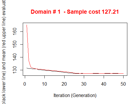
Figure 5: Optimization step for lead concentration with 3 strata

In listing 1 the structure of the optimized strata is reported. The total sample size is 128.

Listing 1: SamplingStrata optimized strata

⬇

Domain Stratum Population Allocation SamplingRate Lower_X1 Upper_X1

1 1 1 1360 53 0.038906 0.0000 101.6446

2 1 2 1073 43 0.039848 101.7265 198.1577

3 1 3 670 32 0.047223 198.4284 502.9274

Listing 2: Ospats optimized strata

⬇

Domain Stratum Population Allocation SamplingRate Lower_X1 Upper_X1

1 1 1 1370 54 0.039416 0.0000 103.9439

3 1 3 1065 43 0.040376 101.9914 198.7357

2 1 2 668 32 0.047904 197.5290 502.9274

If we run Ospats on the same input, we obtain a solution that, suitably elaborated in order to be comparable, is reported in listing 2. It can be seen that strata are slightly overlapping (when the strata obtained by SamplingStrata are never). The total sample size is 129, practically equivalent to the one determined by SamplingStrata. Also the allocations in the strata are almost the same.

We run both softwares a second time with a different number of strata (5). Increasing the number of strata does not change the substantial equivalence of the two approaches in terms of allocation (it is 112 for SamplingStrata and 115 for Ospats), but the resulting stratifications are noticeably different, as it can be seen by Figure 6.

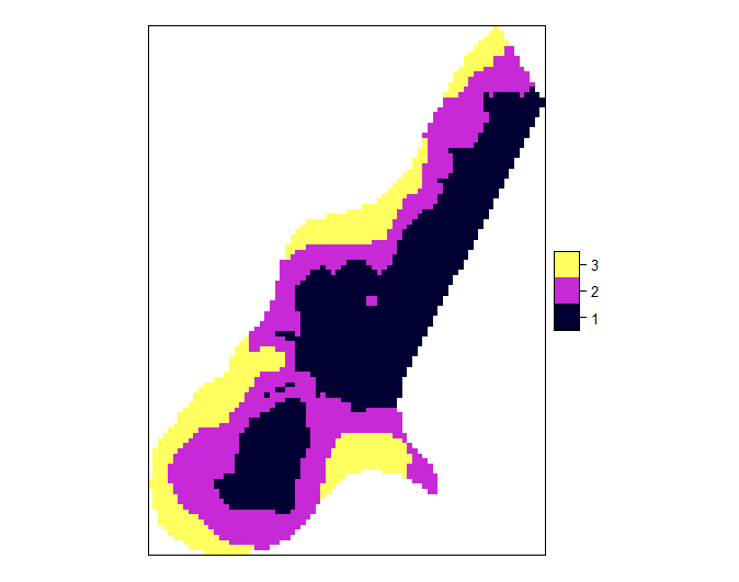
(a) SamplingStrata stratification (3 strata)

(b) Ospats stratification (3 strata)

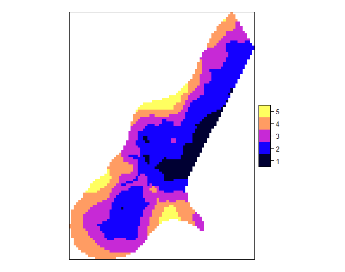
(c) SamplingStrata stratification (5 strata)

(d) Ospats stratification (5 strata)

Figure 6: Comparison of SamplingStrata and Ospats stratifications

The extension from the univariate to the multivariate case is straightforward. We now consider four different target estimates, i.e. the total concentration of all metals (cadmium, copper, lead and zinc) in the Meuse area. After producing variograms and models for each one of the target cariables, we are able to predict their concentration for each point in the grid, together with the error prediction, obtaining this work dataframe:

⬇

df <- NULL

df$cadmium.pred <- preds.cadmium$cadmium.pred

df$cadmium.var <- preds.cadmium$cadmium.var

df$copper.pred <- preds.copper$copper.pred

df$copper.var <- preds.copper$copper.var

df$lead.pred <- preds.lead$lead.pred

df$lead.var <- preds.lead$lead.var

df$zinc.pred <- preds.zinc$zinc.pred

df$zinc.var <- preds.zinc$zinc.var

# df$dom <- meuse.grid@data$soil

df$dom <- 1

df <- as.data.frame(df)

df$id <- meuse.grid$id

head(df)

# cadmium.pred cadmium.var copper.pred copper.var lead.pred lead.var

# 7.917987 7.007012 65.64426 331.6897 265.9674 7043.944

# 8.308433 6.482721 69.01170 308.4855 267.2160 6403.047

# 7.898212 6.661317 66.93037 319.6262 260.5370 6574.794

# 7.281627 6.828875 63.61440 326.8032 248.9653 6770.737

# 8.824362 5.748581 74.34104 245.6440 269.2219 5744.181

# 8.333077 6.009188 71.27280 278.8897 261.5889 5909.198

# zinc.pred zinc.var

# 898.3354 67350.56

# 918.6911 59349.98

# 877.8272 61860.84

# 818.0511 64442.07

# 949.7147 49761.03

# 899.6006 52859.14

We can now proceed with the optimization step in SamplingStrata. As preliminary steps we prepare the precision constraints and sampling frame dataframes:

⬇

cv

# DOM CV1 CV2 CV3 CV4 domainvalue

# 1 DOM1 0.05 0.05 0.05 0.05 1

frame <- buildFrameSpatial(df=df,

id="id",

X=c("cadmium.pred","copper.pred","lead.pred","zinc.pred"),

Y=c("cadmium.pred","copper.pred","lead.pred","zinc.pred"),

variance=c("cadmium.var","copper.var","lead.var","zinc.var"),

lon="lon",

lat="lat",

domainvalue="dom")

The parameter range is now a vector of values:

⬇

range <- c(fit.vgm.cadmium$var_model$range[2],

fit.vgm.copper$var_model$range[2],

fit.vgm.lead$var_model$range[2],

fit.vgm.zinc$var_model$range[2])

In order to "explore" what would be a suitable number of strata in the final solution, we execute the function KMeansSolutionSpatial, that applies a kmeans-based clustering method in order to find a quick solution in correspondence of different numbers of strata, starting from 2 ending to a 10:

⬇

kmeans <- KmeansSolutionSpatial(frame,

fitting=c(1,1,1,1),

range=range,

kappa=1,

gamma=0,

errors=cv,

maxclusters = 10)

Figure 7: Kmeans solutions up to 10 strata

As shown in Figure 7 there is no sensible reduction in sample size after 5 strata, so we choose to set nStrata equal to 5 in the optimization step.

⬇

set.seed(4321)

solution <- optimStrata (

method="spatial",

errors=cv,

framesamp=frame,

iter = 50,

pops = 10,

nStrata = 5,

fitting = c(1,1,1,1),

range = range,

kappa = 1,

writeFiles = FALSE,

showPlot = TRUE,

parallel = FALSE

)

Figure 8: Optimization step for 4 metals concentration with 5 strata

In listing 3 the structure of the optimized strata is reported. The total sample size is 219. The first target estimate (cadmium concentration) is the one that contributes most to the overall sample size: in fact its expected CV is just on the limit of 5% set by the precision constraints.

⬇

expected_CV(solution$aggr_strata)

# cv(Y1) cv(Y2) cv(Y3) cv(Y4)

# 0.05 0.028 0.033 0.033

Listing 3: SamplingStrata optimized strata (multivariate case)

⬇

Domain Stratum Population Allocation SamplingRate Lower_X1 Upper_X1 Lower_X2 Upper_X2

1 1 1 804 78 0.096891 0.000000 1.446959 0.00000 38.97286

2 1 2 965 92 0.095770 0.000000 3.802026 15.50852 73.20976

3 1 3 723 74 0.101837 1.175621 5.916244 28.05583 68.40705

4 1 4 437 46 0.105043 3.479107 8.731853 34.25202 80.43462

5 1 5 174 19 0.106353 5.440594 12.303164 46.90210 120.70553

Lower_X3 Upper_X3 Lower_X4 Upper_X4

1 0.00000 89.1031 0.0000 177.3007

2 46.84002 170.2959 177.4111 380.9390

3 107.15412 249.7760 381.4216 649.5135

4 135.71557 317.1282 649.6953 906.9500

5 219.99896 462.6618 908.4930 1537.8878

The resulting strata are visualized in Figure 9

Figure 9: Final strata in multivariate case

4.2 Case study 2: Census Enumeration Areas Frame

In this case study we will consider a sampling frame containing Census Enumeration Areas (EA’s) as selection units: in particular, the 2,234 EA’s included in Italian Municipality of Bologna. In this basic application, we consider as associated information only the total amount of population and of foreign residents. Population P is continuously updated by the Population Register, but here we use the last 2011 Population Census data. Territorial distribution is shown in Figure 10.

(a) Population

(b) Foreign residents

Figure 10: Territorial distribution in the 2,234 Bologna EA’s

The setting for the study is the following:

• the aim is to design a sample survey whose target is to produce estimates on the size of a given sub-population in the same Bologna territory, i.e. those of the foreign residents;

• data on sub-populations are available with a temporal lag (for instance, at the last Census) or on a subset of EA’s (by means of a non optimized sample): in this case, we consider the second option, in line with the Istat Permanent Census, and will draw a simple random sample with sampling rate equal to 0.2;

• using data on total population (P1) and foreign residents (ST1) for the EA’s where they are jointly available, it is possible to estimate different models, in particular:

  1. Linear Model;

  2. Kriging;

  3. Spatial Linear Model;

• having set precision constraints on one or more target estimates of the sub-population of interest, the best stratification of the frame is obtained by running three different optimization steps, one for each of the above models;

• a compared evaluation of the three different solutions is obtained by simulating the selection of 1,000 samples, calculating for each of them the target estimates and finally deriving the coefficients of variation.

4.2.1 Application on real data

Linear Model

⬇

lm_1 <- lm(ST1 ~ P1,data=spoints_samp)

summary(lm_1)

\# Coefficients:

\# Estimate Std. Error t value Pr(>|t|)

\# (Intercept) -0.053350 0.982107 -0.054 0.957

\# P1 0.118006 0.004238 27.844 <0.0000000000000002 ***

\# —

\# Residual standard error: 15.41 on 465 degrees of freedom

\# Multiple R-squared: 0.6251, Adjusted R-squared: 0.6243

(a)

(b)

Figure 11: Linear model between foreign residents sub-population and total population

As for the distribution of residuals, see Figure 11. It is quite evident the presence of heteroscedasticity and the non-normality of residuals distribution. For this reason, we proceed to compute the heteroscedasticity index and related variance for each one of the three different models, and give corresponding values as input to the optimization steps.

We calculate the heteroscedasticity index and related variability accordingly to the Linear Model (see Figure 13):

⬇

gamma_sigma_1 <- computeGamma(e=summary(lm_1)$residuals,

x=spoints_samp@data$P1,nbins=6)

gamma_sigma_1

# gamma sigma r.square

# 0.6146480 0.6210120 0.9662238

where the first value is the heteroscedasticity index, and the second is the standard deviation

Figure 12:

Figure 13: Distribution of residuals and heteroscedasticity model

We build the sampling frame in this way:

⬇

id X1 Y1 domainvalue lon lat ST1 P1

1164 64 64 1 686797.2 4928305 8 64

300 192 192 1 686739.8 4932537 42 192

1791 190 190 1 684180.3 4929655 27 190

309 350 350 1 687154.7 4932146 131 350

895 0 0 1 682919.1 4931359 0 0

1750 599 599 1 690758.9 4929418 107 599

that is, both stratification variable X1 and target variable Y1 have been set equal to the population total P1.

Having fixed a precision constraint of 3% on the target variable, the first optimization is the one making direct use of the linear model, using the method continuous:

⬇

model <- NULL

model$type[1] <- "linear"

model$beta[1] <- summary(lm_1)$coefficients[2]

model$gamma[1] <- gamma_sigma_1[1]

model$sig2[1] <- gamma_sigma_1[2]^2

model <- as.data.frame(model)

model

# type beta gamma sig2

# 1 linear 0.1180064 0.614648 0.3856559

set.seed(1234)

solution1 <- optimStrata (

method="continuous",

errors=cv,

framesamp=frame,

model=model,

nStrata = 5)

This solution yields a sample size of 400. We now proceed to draw 1,000 samples and calculate the real CV for both the Y1 variable and for the real target variable, ST1:

⬇

framenew <- solution1$framenew

outstrata <- solution$aggr_strata

framenew$Y2 <- framenew$TARGET

val1 <- evalSolution(framenew, outstrata, nsampl=1000)

val1$coeff_var

# CV1 CV2 dom

# 1 0.0094 0.029 DOM1

The CV related to P1 is much lower that the required 3%, but we see that the CV related to our true target variable (ST1) is compliant (2.9%).

Kriging

We move now to the approach based on the use of Kriging. First, we obtain the model in this way:

⬇

# Variogram

v <- variogram(ST1 ~ P1, data=spoints_samp, cutoff=3000, width=3000/30)

# Estimation of psill, range and nugget with automap

fit.vgm = autofitVariogram(ST1 ~ P1, spoints_samp,

model = c("Exp", "Sph", "Mat" ))

plot(v, fit.vgm$var_model)

fit.vgm$var_model

# model psill range kappa

# 1 Nug 114.3363 0.000 0.0

# 2 Mat 135.2903 1232.796 0.2

# Prediction

g <- gstat(NULL, "v", ST1 ~ P1, spoints_samp)

v <- variogram(g)

v.fit <- fit.lmc(v, g,

vgm(psill=fit.vgm$var_model$psill[2],

model=fit.vgm$var_model$model[2],

range=fit.vgm$var_model$range[2],

nugget=fit.vgm$var_model$psill[1]))

preds <- predict(v.fit, Comune_BO_geo)

We calculate the heteroscedasticity index and standard deviation of errors in this way:

⬇

gamma_sigma_2 <- computeGamma(e=lm_pred$residuals[camp],

x=frame1$P1[camp],

nbins=6)

gamma_sigma_2

# gamma sigma r.square

# 0.5100489 0.9401730 0.9394493

and calculate prediction errors in this way:

⬇

frame$var1 <- gamma_sigma_2[2]^2 * (frame1$P1^(2*gamma_sigma_2[1]))

Once assigned to the frame the predicted values and the prediction errors to each unit in the frame, we calculate the fitting of the model in this way:

⬇

# Compute fitting

lm_pred <- lm(ST1 ~ pred,data=frame)

summary(lm_pred)$r.squared

# [1] 0.6351977

We can now proceed with the optimization step using the method spatial:

⬇

frame$var1 <- preds$v.var

solution2 <- optimStrata (

method="spatial",

errors=cv,

framesamp=frame,

nStrata = 5,

fitting = summary(lm_pred)$r.squared,

range = fit.vgm$var_model$range[2],

kappa = 1)

The sample size is now 330, much lower than the previous one, and the expected CV on the target variable is slightly above the desired 3%, as it is 3.2%. Once equalized (that is, once increased the sample size to the same one of the Linear Model) it reduces to 2.85%.

Spatial Linear Model

Finally, we make use of third approach, the one based on the Spatial Linear Model:

⬇

lm_2 <- lm(ST1 ~ P1 + P1W, data=frame[camp,])

summary(lm_2)

# Coefficients:

# Estimate Std. Error t value Pr(>|t|)

# (Intercept) 0.231107 1.457822 0.159 0.874

# P1 0.118487 0.004616 25.667 <0.0000000000000002 ***

# P1W -0.002018 0.007638 -0.264 0.792

# Residual standard error: 15.42 on 464 degrees of freedom

# Multiple R-squared: 0.6251, Adjusted R-squared: 0.6235

We observe that the value of the coefficient related to P1W is very small, thus indicating a limited presence of spatial auto-correlation.

We calculate heteroscedasticity and variability:

⬇

gamma_sigma_3 <- computeGamma(e=(frame$target[camp] -

predict(lm_2,data=frame[camp,])),

x=spoints_samp@data$P1,nbins=6)

# gamma sigma r.square

# 0.6132473 0.6257764 0.9654370

and calculate the value of the range:

⬇

v2 <- variogram(res_spatial ~ 1, data=spoints_samp)

fit.vgm2 = autofitVariogram(res_spatial ~ 1, spoints_samp,

model = c("Exp","Sph","Mat"))

fit.vgm2$var_model

# model psill range kappa

# 1 Nug 114.3825 0.000 0.0

# 2 Mat 135.2430 1232.444 0.2

We can now proceed with the optimization step:

⬇

model

# type beta beta2 sig2 range gamma fitting

# 1 spatial 0.1184873 -0.002018293 0.3915961 1232.444 0.6132473 0.6251384

solution3 <- optimStrata (

model="continuous",

errors=cv,

framesamp=frame,

model=model,

nStrata = 5)

obtaining a total allocation of 393. As in the case of the Linear Model, the expected CV on the target is compliant with the precision requirement. Once equalized, it reduces to 2.89%.

As an example of a resulting stratification, we report the one obtained with the Kriging Model in Figure 14, together with the 330 sampled EA’s.

(a) Stratified EA’s

(b) Sampled EA’s

Figure 14: Stratification obtained with the Kriging Model

The structure of the obtained strata, in terms of boundaries, together with allocation and sampling rate, is reported in Listing 4.

Listing 4: Results of the application of the three models

⬇

*** Linear model (gamma/sigma/R2 = 0.614648 0.621012 0.9662238 ) ***

R squared: 0.625082

Sample size 400

Domain Stratum Population Allocation SamplingRate Lower_X1 Upper_X1

1 1 1 689 28 0.040516 0 36

2 1 2 617 82 0.133399 37 137

3 1 3 433 92 0.212173 138 248

4 1 4 421 126 0.300094 250 432

5 1 5 174 72 0.414277 433 1072

CV(P1) CV(ST1)

0.0094 0.029

*** Kriging (gamma/sigma/R2 = 0.5006069 0.9888317 0.9372327 ) ***

R squared: 0.6351977

Sample size 330

Domain Stratum Population Allocation SamplingRate Lower_X1 Upper_X1

1 1 1 685 37 0.054042 0.00 4.12

2 1 2 534 57 0.107322 4.15 13.94

3 1 3 467 75 0.161391 13.97 27.98

4 1 4 428 93 0.218032 28.04 49.32

5 1 5 220 68 0.307086 49.49 123.91

CV(P1) CV(ST1)

0.0105 0.0321

… with the same sample size than Linear Model

CV(P1) CV(ST1)

0.0088 0.0285

*** Spatial model (gamma/sigma/R2 = 0.6241951 0.5883335 0.9638095 ) ***

R squared: 0.6251384

Sample size 393

Domain Stratum Population Allocation SamplingRate Lower_X1 Upper_X1

1 1 1 689 29 0.042281 0 36

2 1 2 617 81 0.131964 37 137

3 1 3 433 88 0.203478 138 248

4 1 4 421 123 0.291982 250 432

5 1 5 174 72 0.413850 433 1072

CV(P1) CV(ST1)

0.009 0.0304

… with the same sample size than Linear Model

CV(P1) CV(ST1)

0.0095 0.0289

4.2.2 Simulation

The results obtained in the application to real data indicate that:

• both Linear Model and Spatial Linear Model are compliant with the precision requirement of 3%, while Kriging is slightly over;

• conversely, in terms of sample size, the Kriging is the one with the minimum;

• once equalized (that is, after rendering equal all the sample sizes of the three solutions), the expected CVs are about the same, with a minimum for the Kriging;

• the structure of the obtained optimized strata varies from one solution to another, both in terms of strata boundaries and allocations.

The substantial equivalence of the results obtained with three models is probably due to a weak spatial correlation of the variable of interest.

In order to analyse the contribution of spatial component in the overall variance to results obtainable by different models, we decided to carry out a simulation by generating for each EA in the frame an artificial variable $Z$, characterized by a high spatial correlation, by making use of the following equation:

$Z=Y\beta_{1}+WY\beta_{2}+u\cdot Y^{\gamma}$

In our case $Y$ is the population P1 in each EA, $\beta$ has been set equal to 1, $W$ is the weighted contiguity matrix, and the errors $\epsilon$ are spatially correlated and affected by heteroscedasticity. The error term $u$ has been generated as a Gaussian random field, whose parameters are the following:

1. the covariance model is exponential;

2. the error variance has been set equal to 2000;

3. the range of spatial correlation has been set to 2000;

4. the values of heteroscedasticity index ($\gamma$) ranges from 0 to 0.7 with a step equal to 0.05.

In Table 1 and in Figure 15 the results of the simulation are reported.

		Linear		Kriging			Spatial
Run	Heter.lev.	n	CV	n	CV	CV eq.	n	CV	CV eq.
1	0	319	0.0167	36	0.0399	0.0125	105	0.0299	0.0162
2	0.05	254	0.0192	37	0.0407	0.0148	110	0.0300	0.0192
3	0.10	275	0.0188	37	0.041;	0.0139	120	0.0304	0.0187
4	0.15	297	0.0305	34	0.0435	0.0131	134	0.0286	0.0186
5	0.20	338	0.0297	38	0.0411	0.0126	156	0.0300	0.0195
6	0.25	395	0.0282	44	0.0397	0.0128	188	0.0300	0.0194
7	0.30	462	0.0281	67	0.0365	0.0128	230	0.0301	0.0194
8	0.35	530	0.0278	78	0.0366	0.0127	276	0.0292	0.0200
9	0.40	591	0.0270	95	0.037;	0.0124	341	0.0297	0.0206
10	0.45	653	0.0220	119	0.0361	0.0135	402	0.0287	0.0220
11	0.50	690	0.0255	146	0.0352	0.0137	456	0.0286	0.0220
12	0.55	707	0.0234	171	0.0349	0.0146	505	0.0299	0.0241
13	0.60	709	0.0238	196	0.036;	0.0149	467	0.0336	0.0250
14	0.65	695	0.0255	223	0.0349	0.0173	478	0.0344	0.0279
15	0.70	676	0.0268	240	0.0368	0.0184	483	0.0353	0.0287

Table 1: Simulation results.

We see that:

1. as for the overall sample sizes required by the three models (see Figure 15(a)), those obtained by the Kriging are always the minimum, followed by the Spatial Linear Model, while the Linear Model is characterized by very high levels of smple size;

2. in terms of resulting expected coefficient of variation on the target variable (Figure 15(b)), the Spatial Linear Model is the only one whose expected CV are in line with the precision requirement; the Linear Model is the one that yields the minimum values, while the Kriging produces the highest values;

3. finally, considering the equalized expected CV (the CV that is obtained when the sample size of Kriging and Spatial Linear Model are increased to the one of the Linear Model), the Kriging is always the best, while the other two are characterized by near the same values.

As a first indication, we can conclude that:

• if the aim is to minimize the overall sample size, Kriging is the right choice: there is no warranty that the precision constraint will be respected, but the efficiency of the solution is maximized;

• if conversely we want to stick to the precision constraint, the Spatial Linear Model should be preferred, because it has to be expected that the sample size is the one actually needed in order to be compliant.

(a) Performance in terms of sampling size

(b) Performance in terms of CV on target variable

(c) Performance in terms of equalized CV on target variable

Figure 15: Results of simulation

5 Conclusions and future work

The functionalities of the package SamplingStrata have been enriched by new developments, having the aim to increase its effectiveness and efficiency, and to extend its applicability.

The changes in the Genetic Algorithm when method "atomic" is used, respond to the need of increasing its computational performance.

The new method "continuous" allows to produce strata that are more interpretable and manageable, and in some cases also more efficient.

The handling of anticipated variance permits to compute variance in strata in a more correct way, taking into account the difference between available variables in the frame, and the variables that are the real target of the sampling survey. Very important to this aim is the consideration of heteroscedasticity of residuals, and the new function computeGamma allows to estimate its value.

The extension to the case where units in the frame can be georeferenced or geocoded covers the more and more important field of spatial sampling. The two alternatives provided, i.e. (i) the extension of model types to the ’spatial’ linear model in the handling of anticipated variance, and (ii) the development of a method, "spatial", both allow to take into account the spatial auto-correlation when calculating variance in strata, thus increasing the correctness and efficiency of optimized solutions. In the reported case studies, the applicability of these new functionalities has been illustrated, though there is not yet a clear evidence of what may be the best one. In our opinion, we need to investigate better the use of the different variants of the Spatial Linear Model.

Another required development will concern sample selection techniques peculiar of spatial sampling. Once optimal strata have been defined, it would be important to select units inside them by using techniques (as, for instance, grid sampling), that ensure to harness the spatial auto-correlation at the maximum extent.

References

- Baillargeon & Rivest (2014) Baillargeon, S., & Rivest, L.-P. (2014). stratification: Univariate Stratification of Survey Populations. R package version 2.2-5.
- Ballin & Barcaroli (2014) Ballin, M., & Barcaroli, G. (2014). Joint determination of optimal stratification and sample allocation using genetic algorithm. Survey Methodology, 39, 369–393.
- Ballin & Barcaroli (2016) Ballin, M., & Barcaroli, G. (2016). Optimization of stratified sampling with the r package samplingstrata: applications to network data. In M. Dehmer, Y. Shi, & F. Emmert-Streib (Eds.), Computational Network Analysis with R: Applications in Biology, Medicine and Chemistry chapter 5. (pp. 125–150). Wiley.
- Ballin & Barcaroli (2020a) Ballin, M., & Barcaroli, G. (2020a). Optimization of sampling strata with the SamplingStrata package. R package version 1.5-1.
- Ballin & Barcaroli (2020b) Ballin, M., & Barcaroli, G. (2020b). Use of models in SamplingStrata. R package version 1.5-1.
- Ballin et al. (2018) Ballin, M., Barcaroli, G., Masselli, M., & Scarnò, M. (2018). Redesign sample for Land Use/Cover Area frame Survey (LUCAS) 2018. Statistical Working Papers Eurostat.
- Barcaroli (2014) Barcaroli, G. (2014). SamplingStrata: An R package for the optimization of stratified sampling. Journal of Statistical Software, 61, 1–24.
- Barcaroli et al. (2020) Barcaroli, G., Ballin, M., Odendaal, H., Pagliuca, D., Willighagen, E., & Zardetto, D. (2020). SamplingStrata: Optimal Stratification of Sampling Frames for Multipurpose Sampling Surveys. R package version 1.5-1.
- Bethel (1989) Bethel, J. (1989). Sample allocation in multivariate surveys. Survey Methodology, 15, 47–57.
- Gräler et al. (2016) Gräler, B., Pebesma, E., & Heuvelink, G. (2016). Spatio-temporal interpolation using gstat. The R Journal, 8, 204–218.
- de Gruijter et al. (2015) de Gruijter, J., Minasny, B., & McBratney, A. (2015). Optimizing stratification and allocation for design-based estimation of spatial means using predictions with error. Journal of Survey Statistics and Methodology, (pp. 19–42).
- de Gruijter et al. (2019) de Gruijter, J., Wheeler, I., & Malone, B. (2019). Using model predictions of soil carbon in farm-scale auditing - a sofwtare tool. Agricultural Systems, (pp. 24–30).
- Henry & Valliant (2006) Henry, K., & Valliant, R. (2006). Comparing Strategies to Estimate a Measure of Heteroscedasticity, . https://www.irs.gov/pub/irs-soi/06rppphenry.pdf.
- Hiemstra et al. (2008) Hiemstra, P., Pebesma, E., Twenhofel, C., & Heuvelink, G. (2008). Real-time automatic interpolation of ambient gamma dose rates from the dutch radioactivity monitoring network. Computers & Geosciences, . DOI: http://dx.doi.org/10.1016/j.cageo.2008.10.011.
- Knaub (2019) Knaub, J. (2019). Estimating the Coefficient of Heteroscedasticity, . https://www.researchgate.net/profile/James_Knaub.
- Lisic et al. (2018) Lisic, J., Sang, H., Zhu, Z., & Zimmer, S. (2018). Optimal stratification and allocation for the june agricultural survey. Journal of Official Statistics, 34, 121–148.
- O’Luing et al. (2017) O’Luing, M., Prestwich, S., & Tarim, S. A. (2017). Constructing strata to solve sample allocation problems by grouping genetic algorithm. arXiv:1709.03076, .
- O’Luing et al. (2019) O’Luing, M., Prestwich, S., & Tarim, S. A. (2019). A grouping genetic algorithm for joint stratification and sample allocation designs. Survey Methodology, 45, 513–531.
- Pebesma (2019) Pebesma, E. (2019). The meuse data set: a brief tutorial for the gstat R package. R package gstat version 2.0-2.
- Pebesma (2004) Pebesma, E. J. (2004). Multivariable geostatistics in S: the gstat package. Computers & Geosciences, 30, 683–691.
- Pebesma & Bivand (2005) Pebesma, E. J., & Bivand, R. S. (2005). Classes and methods for spatial data in R. R News, 5, 9–13.