Geometry optimisation of a transparent axisymmetric ion trap for the MORA project

Abstract

In the frame of the project MORA (Matter’s Origin from the Radio Activity of trapped and oriented ions), a transparent axially symmetric radio-frequency ion trap (moratrap) was designed in order to measure the triple correlation parameter $D$ in nuclear $\beta-$decay of laser-polarised ions. The trap design was inspired from the lpctrap geometry, operated at GANIL from 2005 to 2013. In a real (non-ideal) Paul trap, the quadrupole electric potential is not perfect leading to instabilities in ion motion and therefore affecting the overall trapping efficiency. This paper presents a numerical method aiming to optimise the geometry of a trap. It is applied to moratrap in order to improve the trapping efficiency and to enlarge the axial transparent solid angle compared to lpctrap. In the whole optimisation process, numerical computation of electric potential and field was carried out using an electrostatic solver based on boundary element method (BEM). The optimisation consisted in minimising an objective function (fitness function) depending on higher order multipoles of the potential. Finally, systematic changes of trap dimensions and electrode displacements were applied to investigate geometrical effects on the potential quality.

1 Introduction

Precision measurements in nuclear $\beta-$decay provide a remarkable tool to improve the accuracy of Standard Model (SM) parameters and to search for New Physics (NP) beyond, at the low energy frontier Gonzales:2019 . In particular, the search for new sources of CP (Charge Parity) violation is one of the requirements to explain the matter$-$antimatter asymmetry observed in the universe, according to Sakharov’s criteria Sakharov:1967 . This search can be achieved in nuclear $\beta-$decay by measuring the triple correlation between the parent nucleus spin ($\vec{J}$), electron momentum ($\vec{p}_{e}$), and neutrino momentum ($\vec{p}_{\nu}$): $D\left\langle\vec{J}\right\rangle\cdot(\vec{p}_{e}\times\vec{p}_{\nu})$. This triple correlation is sensitive to T (Time) reversal violation and thus to CP violation thanks to CPT conservation. Such a violation would be quantified by a non-zero $D$ value, experimentally determined from an asymmetry in the $\beta$-recoil angular distribution measured in a plane perpendicular to $\vec{J}$ for two opposite directions of this nucleus orientation. In this context, the new project MORA Delahaye:2018 aims to measure the triple-correlation $D$ coefficient in the $\beta$-decay of laser-polarised ${}^{23}\mbox{Mg}^{+}$ and ${}^{39}\mbox{Ca}^{+}$ ions confined in a Paul trap applying a quadrupole radio frequency (RF) field. The use of Paul traps is considered as an innovative technique in precision measurements of correlation coefficients in nuclear $\beta-$decay in the SM framework Sternberg:2015 ; Brodeur:2016 . One example is the transparent Paul trap lpctrap used in the measurement of the $\beta-\nu$ correlation coefficient, $a_{\beta\nu}$, in the decay of different nuclei Ban:2013 ; Fabian:2014 ; Lienard:2015 ; Delahaye:2019 .

The central element of the MORA apparatus is a transparent Paul trap (moratrap), which will be used to confine singly charged radioactive ions, coupled to a laser system allowing to polarise the nucleus by optical pumping. As shown in Fig. 1, moratrap, which will be installed in a vacuum chamber, is surrounded by four pairs of electron and recoil ion detectors arranged alternately in an octagonal geometry in the azimuthal plane of the trap and allowing close to $2\pi$ azimuthal coverage. Two annular silicon detectors (not visible on the figure) located on the trap axis will monitor the polarisation degree thanks to $\beta$ asymmetry measurement.

The RF potential generated in the trapping volume or region of interest (ROI) is not perfectly a quadrupole but contains some small amplitude, higher order electric multipole components which disturb the ion’s motion. Since the potential in the ROI depends on the electrodes shape and on the applied voltages, an optimisation of the trap geometry is mandatory to reduce the higher order harmonics and to generate an optimised quadrupole potential.

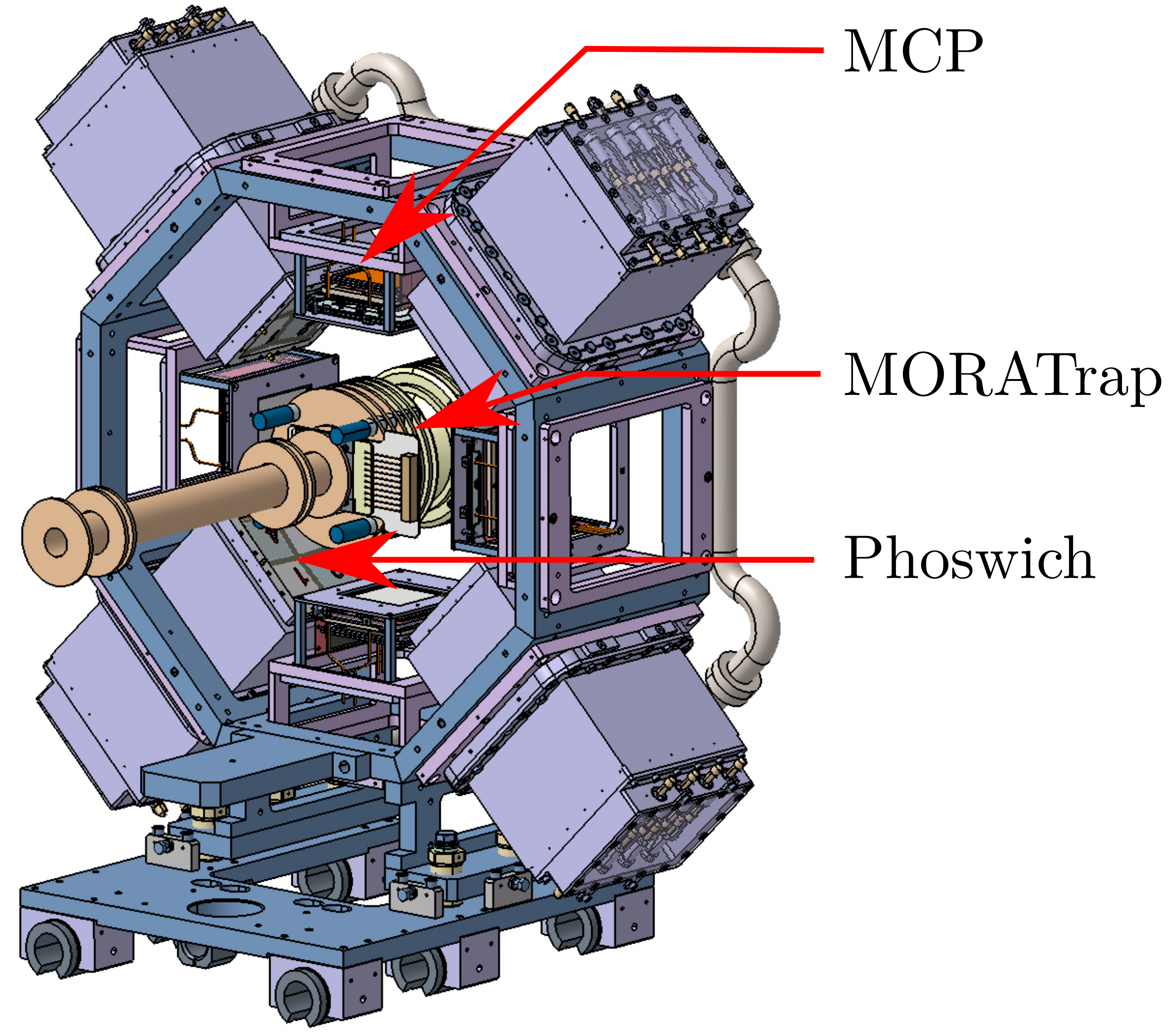
Figure 1: moratrap setup overview showing the location of the ion trap in the centre surrounded by 4 beta detectors (Phoswich) and 4 recoil ion detectors (MCP).

In this work, we will describe an efficient method to optimise the moratrap geometry, using two electrostatic solvers developed at LPC Caen. Our trap is a three dimensional transparent Paul trap, inspired from the lpctrap geometry, where the electrodes have been modified from an ideal Paul trap to allow the detection of $\beta-$ decay products in a large solid angle around the azimuthal plane and obtain an efficient injection of the ion bunches. By optimising the geometry, we aim to reach a quadrupole potential of higher quality, to minimise the ion losses from the trap and to increase the trapping lifetime and the space charge capacity. Such improvements are mandatory to reach the statistics required in the MORA experiment to search for NP.

The potential of an ideal Paul trap is commonly defined in cylindrical ($r$, $z$) coordinates as:

$$V_{\mathrm{ideal}}(r,z,t)\,=\,V_{0}\,\cos(\Omega t)\,\frac{r^{2}\,-\,2\,z^{2}}{2\,r_{0}^{2}},$$ (1)

where $V_{0}$ is the amplitude of the RF voltage, $\Omega=2\pi f$ its pulsation, and $r_{0}$ a distance parameter. 3D Paul traps usually approximate the ideal Paul trap by using electrodes consisting of one ring and two end caps, whose surfaces form truncated hyperboloids (see for example Fig. 1 in Delahaye:2019 ). In such a configuration, $r_{0}$ is the distance of the ring surface to the centre of the trap. In geometries which significantly depart from the ideal trap, one can define an effective trapping radius $r_{\mathrm{eff}}$ which contains the region where the quadrupole field still sufficiently dominates, so that ion trajectories are still stable in standard conditions defined for the ideal potential. This region is defined in Delahaye:2019 as the region for which the contribution to the potential from harmonics of higher order than the quadrupole one, are still below a few percents. The conditions for stability of an ion of mass $m$ and charge $q$ in an ideal Paul trap, in the absence of DC field, are defined with respect to the Mathieu parameter $q_{z}$:

$$q_{z}\,=\,\frac{4\,q\,V_{0}}{m\,r_{0}^{2}\,\Omega^{2}}.$$ (2)

In the first stability region, $|q_{z}|<0.908$ March:2005 . In the pseudo-potential approximation limit, valid for small $q_{z}$ values, one can define a pseudo-potential depth $D_{z}$ (resp. $D_{r}$) for the $z$ (resp. $r$) dimension:

$$D_{z}\,=\,\frac{q_{z}\,V_{0}}{8}\,=\,2\,D_{r}.$$ (3)

In this model, the maximal charge density $\rho_{\mathrm{max}}$ the Paul trap can hold is

$$\rho_{\mathrm{max}}\,=\,\frac{3\,\varepsilon_{0}\,D_{z}}{z_{0}^{2}},$$ (4)

where $\varepsilon_{0}$ is the vacuum permittivity and $z_{0}\,=\,r_{0}/\sqrt{2}$ is the distance of the end caps from the trap centre. From Eqs. (2) to (4) and considering the fact that experimentally one usually fixes a Mathieu parameter in the middle of the stability diagram $q_{z}\,\simeq\,0.4$ Delahaye:2019 , the maximal charge capacity $Q_{\mathrm{max}}$ a trap can hold directly relates to the product $r_{0}V_{0}$ via the formula:

$$Q_{\mathrm{max}}\,=\,\frac{1}{2}\pi\varepsilon_{0}q_{z}r_{0}V_{0}$$ (5)

in the case of an ideal trap, and

$$Q_{\mathrm{max}}=\frac{1}{2}\pi\varepsilon_{0}q_{z}r_{\mathrm{eff}}V_{\mathrm{eff}}$$ (6)

in the case of a Paul trap with a limited quadrupole region of radius $r_{\mathrm{eff}}$, where $V_{\mathrm{eff}}\,=\,V_{0}\frac{r_{\mathrm{eff}}^{2}}{r_{0}^{2}}$ is the maximum potential at the radius $r_{\mathrm{eff}}$. In order to optimise the charge capacity of the trap for the MORA experiment, the optimisation procedure presented in this article therefore aims at enlarging the trapping region, of radius $r_{\mathrm{eff}}$, given some space constraints on the size of the trap.

Sec. 2 presents the electrostatic solvers necessary to compute the potential from an electrode set and Sec. 3 introduces the harmonics series expansion describing this potential, solution of Laplace’s equation. Sec. 4 details the objective function used in the optimisation procedure whose results are presented and commented in Secs. 5 and 6. Finally, the effects of electrode misalignment on the potential quality are investigated in Sec. 7.

2 Laplace’s solver

The shape of the electric potential generated within a trap depends on both the electrode geometry and their corresponding applied voltages. In order to estimate and optimise this potential, it needs to be accurately computed within the ROI (the trapping region). This is achieved by solving Laplace’s equation in this ROI. For that purpose, the most common approaches use either the finite element method (FEM) or the finite difference method (FDM) which require to mesh both the electrodes and the free space volume. For our study, we have used a home made C++ Laplace’s solver based on the boundary element method (BEM). This solver has been developed by one of us and thoroughly validated with analytic examples and expensive commercial software like simion (FDM) or comsol (FEM). Compare to FEM and FDM, BEM exhibits several advantages: it only requires to mesh the surface of the electrodes and is thus able to achieve higher precision with less computation time and memory requirements. This is especially true for geometries involving electrodes with large aspect ratios (e.g. a very thin thickness for very large length and width) for which the 3D meshing quality would require special care. In addition, BEM can easily deal with open systems as the boundary conditions are inherent to the formalism.

Even if our BEM program also handles dielectric materials, in order to simplify its description, here we shall only concentrate on sets of electrodes with applied voltages. A setup is described by $N_{e}$ electrodes each represented by its surface. The surface of electrode $e\,(e\in[1,N_{e}])$ is meshed in $n_{e}$ flat polygonal cells (triangles, quadrangles, …). The full setup is therefore represented by the set of cells $\mathcal{C}=\left\{\mathcal{C}_{i}:i\in[1,N]\right\}$ where $N=\sum_{e=1}^{N_{e}}n_{e}$ is the total number of cells, each with an a priori unknown associated surface charge density $\sigma_{i}$ assumed constant over the cell surface. The $n_{e}$ cells of electrode $e$ obviously share the same potential applied on the whole electrode. The potential $V_{i}$ of cell $\mathcal{C}_{i}$ centred at position $\mathbf{r}_{i}$ is related to the surface charge densities $\sigma_{j}$ of cells $\mathcal{C}_{j}$ ($j\in[1,N]$) through the superposition principle as:

$$V_{i}\,=\,\sum_{j=0}^{N}\,\frac{\sigma_{j}}{4\pi\varepsilon_{0}}\,\int_{\mathcal{C}_{j}}\frac{1}{\|\mathbf{r}_{i}-\mathbf{r^{\prime}}\|}\mathrm{d}^{2}\mathbf{r^{\prime}}\,=\,\sum_{j=0}^{N}\,Q_{ij}\,\sigma_{j},$$ (7)

where the integral over the surface of cell $\mathcal{C}_{j}$ only depends on $\mathcal{C}_{j}$ shape and on the relative position of the target point $\mathbf{r}_{i}$ with respect to $\mathcal{C}_{j}$ location, as $\sigma_{j}$ is assumed constant over the whole surface of cell $\mathcal{C}_{j}$. An analytic formula has been derived for the integral in Eq. (7). This formula is too complicated to be discussed here and shall be published in a separate article, but it should be emphasised that special care has been taken to suppress numerical instabilities in its evaluation especially when $i=j$ where numerical divergence may occur. Eq. (7) can be written for each cell $\mathcal{C}_{i}$, leading to the following set of $N$ equations:

$$\begin{pmatrix}V_{1}\\ V_{2}\\ \vdots\\ V_{N}\end{pmatrix}=\begin{pmatrix}Q_{1,1}&Q_{1,2}&\cdots&Q_{1,N}\\ Q_{2,1}&Q_{2,2}&\cdots&Q_{2,N}\\ \vdots&\vdots&\ddots&\vdots\\ Q_{N,1}&Q_{N,2}&\cdots&Q_{N,N}\end{pmatrix}\begin{pmatrix}\sigma_{1}\\ \sigma_{2}\\ \vdots\\ \sigma_{N}\end{pmatrix},$$ (8)

where $V_{i}$ are the known potentials applied on electrodes and $\sigma_{i},i\in[1,N]$ are the unknown surface charge densities. The matrix elements $Q_{ij}$ are computed for a given electrode assembly/geometry leading to a dense square matrix on the contrary to FEM and FDM which deal with sparse matrices of much larger dimensions. The presence of a dense matrix requires special algorithms to solve Eq. (8) for the $\sigma_{i}$: a direct solver such as LU decomposition can be used to obtain an exact solution or an approximated solution can also be computed more rapidly with iterative solvers such as CMRH Sadok:1999 . Once the charge densities have been determined, the potential and field components can be evaluated at any location $\mathbf{r}$ in space without interpolation contrary to the FEM and FDM approaches:

$$V(\mathbf{r}) = \sum_{i=0}^{N}\,\frac{\sigma_{i}}{4\pi\varepsilon_{0}}\,\int_{\mathcal{C}_{i}}\frac{1}{\|\mathbf{r}-\mathbf{r^{\prime}}\|}\mathrm{d}^{2}\mathbf{r^{\prime}}$$ (9)

$$\mathbf{E}(\mathbf{r}) = \sum_{i=0}^{N}\,\frac{\sigma_{i}}{4\pi\varepsilon_{0}}\,\int_{\mathcal{C}_{i}}\frac{\mathbf{r}-\mathbf{r^{\prime}}}{\|\mathbf{r}-\mathbf{r^{\prime}}\|^{3}}\mathrm{d}^{2}\mathbf{r^{\prime}}$$ (10)

As for Eq. (7), integrals in Eqs. (9) and (10) are analytically evaluated over the surface of each cell.

For our studies we have used two versions of the solver: a full 3D solver, called electrobem, and a derived version, axielectrobem for axially symmetric problems. In electrobem, a complex 3D setup can be modelled with a thorough set of geometric functions handling predefined shapes (flat polygons, ring, cylinder, cone, torus, …), rotations, translations and symmetry planes as well as fine tuning of mesh properties. This last point is crucial for the precision of the solution. The software can also import pre-computed meshes from the open source, reliable and user friendly gmsh software Geuzaine:2009 . Both gmsh and root Root:1997 may be used to display the geometry. Electric potentials are applied to electrodes and then, once the electrostatic problem has been solved, a complete set of plotting/mapping functions allows to display and/or export the potential and field components in 1D, 2D and 3D as illustrated for instance in Figs. 2 and 3. In axielectrobem, any shape axially symmetric around $z$-axis can be simulated by predefined shapes or by functions ($r=f(z)$). The meshing is done along longitudinal $z-$axis and radial $r-$axis. In this version, the number of cells necessary to model a given axisymmetric setup is substantially smaller than it would be in the 3D version for the same geometry, resulting in a much smaller computation time. axielectrobem is thus particularly well suited for the optimisation of the axially symmetric moratrap and was used in a first phase of our study, whereas the 3D version served in a second phase to estimate the effects, on the trapping potential quality, of possible mechanical misalignment or machining precision which break the setup axisymmetry. Depending on the version, 2D or 3D, the potential inside the trap is expanded differently in terms of multipole coefficients, as shown in next section and in appendix A.

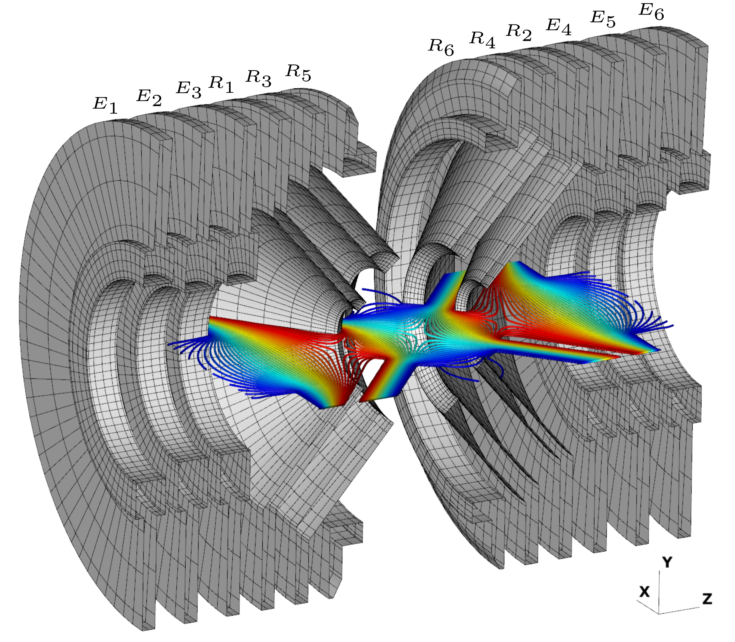
Figure 2: gmsh cross section view of moratrap showing the electrodes along with iso-potential lines obtained with electrobem. The trap consists of three ring electrode pairs ($R_{1}-R_{2}$, $R_{3}-R_{4}$ and $R_{5}-R_{6}$) surrounded by two Einzel lens triplets ($E_{1}-E_{3}$ and $E_{4}-E_{6}$). A more detailed description is given in Sec. 5. The thin black lines on the electrodes delimit the perimeter of the polygonal cells used to solve the electrostatic problem.

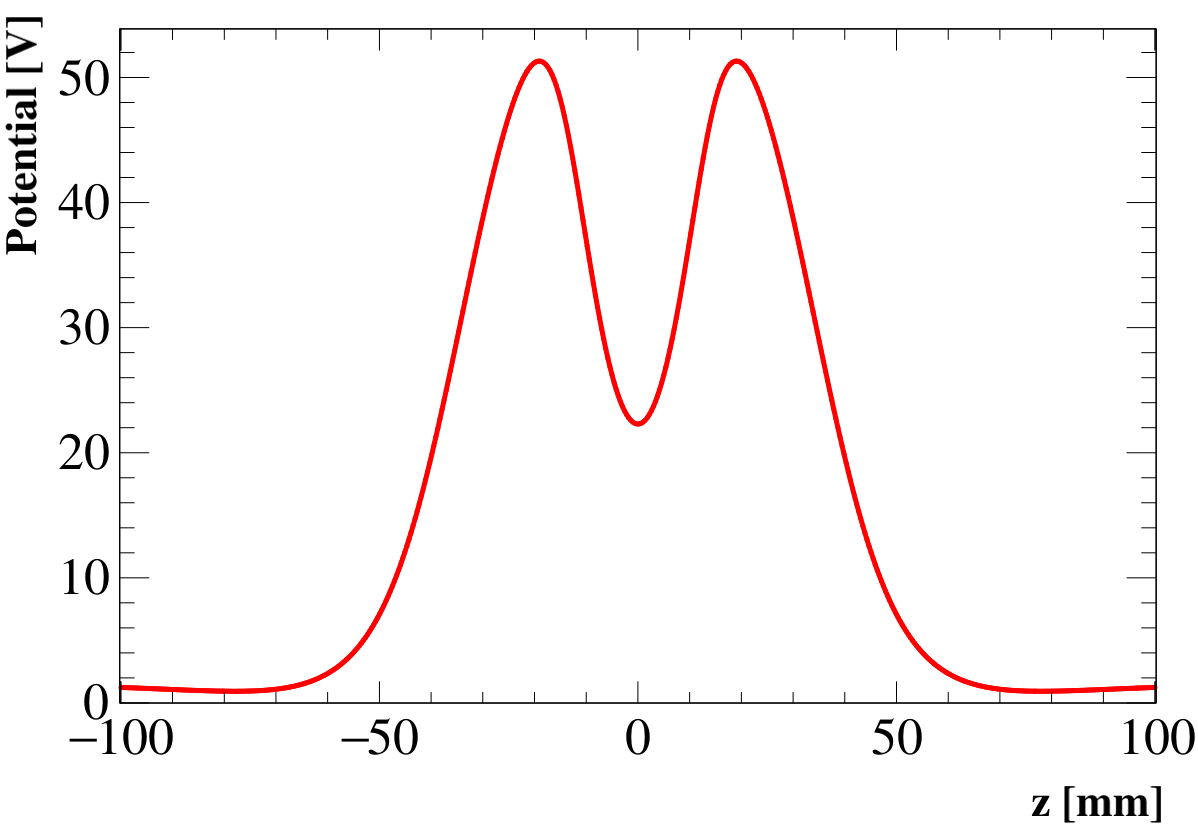
Figure 3: root view of the potential along moratrap axis ($r=0$) computed in axielectrobem for 60 V applied on inner electrodes $R_{1}$ and $R_{2}$, all other ones being grounded.

3 Laplace’s equation: spherical harmonics series expansion

In a source-free region, i.e. in the absence of charges, the electric potential satisfies Laplace’s equation $\Delta V(\rho,\theta,\varphi)\,=\,0$ with $(\rho,\theta,\varphi)$ being the usual spherical coordinates. The solution of this equation edurand , may be expressed in terms of a uniformly convergent Laplace series also known as spherical harmonics series expansion in the following way:

$$V(\rho,\theta,\varphi) = \sum_{n=0}^{\infty}\sum_{m=0}^{n}\!\sqrt{\frac{2n+1}{4\pi}\frac{(n-m)!}{(n+m)!}}\left(\frac{\rho}{R_{0}}\right)^{\!\!n}\!\!P^{m}_{n}(\cos\theta)$$ (11)

$$\times \left[\alpha_{nm}\cos(m\varphi)-\beta_{nm}\sin(m\varphi)\right]$$

$$= \sum_{n=0}^{\infty}\sum_{m=0}^{n}\left(\frac{\rho}{R_{0}}\right)^{\!\!n}\!\!P^{m}_{n}(\cos\theta)$$

$$\times \left[A_{nm}\cos(m\varphi)-B_{nm}\sin(m\varphi)\right],$$

where $P^{m}_{n}(\cos\theta)$ are the associated Legendre functions of the first kind, of degree $n$ and order $m$, and $A_{nm}$ (resp. $B_{nm}$) are the normal (resp. skew) spherical harmonics coefficients ($\alpha_{nm}$ and $\beta_{nm}$ being the corresponding unnormalised harmonics). $R_{0}$ is the convergence radius of the above series expansion, it must be smaller than the distance between the origin ($\rho=0$) and the closest electrode: the region of convergence or the ROI must remain a source free region.

In axisymmetric cases with azimuthal symmetry, the potential does not depend on the $\varphi$ angle and therefore we only keep terms with $m=0$ in the above expansion. Dropping the $m$ index and the $\varphi$ dependence, Eq. (11) reduces to:

$$V(\rho,\theta) = \sum_{n=0}^{\infty}\alpha_{n}\sqrt{\frac{2n+1}{4\pi}}\left(\frac{\rho}{R_{0}}\right)^{\!\!n}P_{n}(\cos\theta)$$ (12)

$$= \sum_{n=0}^{\infty}A_{n}\left(\frac{\rho}{R_{0}}\right)^{\!\!n}P_{n}(\cos\theta)$$

with $P_{n}(\cos\theta)$ the Legendre polynomial of degree $n$ and $A_{n}$ the harmonic coefficient of order $n$ ($\alpha_{n}$ is the corresponding unnormalised harmonics). $A_{0}$ is a constant term for the potential and therefore it does not appear in the field components which enter the ion equations of motion. $A_{1}$ is called the dipole harmonics, $A_{2}$ the quadrupole one and so on for higher orders. The harmonics $A_{2k+1}$ with $k=0,1,2,\dots$ are said to belong to the dipole series whereas harmonics $A_{4k+2}$ with $k=0,1,2,\dots$ are said to belong to the quadrupole series. Because of symmetry reasons, a potential exhibiting a quadrupole behaviour, is more likely to have harmonics from the quadrupole series ($A_{2},\,A_{6},\,A_{10},\dots$) dominant over other higher order terms. One should also notice that the general trend of $A_{n}$ is to decrease with increasing $n$ and that the contribution from $A_{n}$ to the potential is weak close to the origin and increases as $\rho^{n}$. If, in addition to the axial symmetry, a setup exhibits a symmetry plane at $z=0$, then only harmonics $A_{n}$ with even order $n$ will be present in the expansion. The harmonic coefficient $A_{n}$ is obtained by integration over the sphere $S$ of radius $R_{0}$ by:

$$A_{n}\,=\,\frac{2n+1}{4\pi}\!\!\int_{0}^{2\pi}\!\!\mathrm{d}{\varphi}\int_{0}^{\pi}\!\!P_{n}(\cos\theta)\,\,V(R_{0},\,\theta)\,\sin\theta\,\mathrm{d}{\theta}.$$ (13)

After integration over $\varphi$, and assuming a symmetry plane at $z=0$, $A_{n}$ becomes:

$$A_{n}\,=\,(2n+1)\,\int_{0}^{\frac{\pi}{2}}\!P_{n}(\cos\theta)\>V(R_{0},\,\theta)\,\sin\theta\,\mathrm{d}{\theta}.$$ (14)

In order to determine the ${A}_{n}$ coefficients for a given electrode configuration, Eq. (14) is numerically integrated using a 64-nodes Gauss-Legendre quadrature with the potential $V(R_{0},\,\theta)$ calculated on the circle of radius $R_{0}$ at the Gauss-Legendre nodes ($\theta_{i}$) using the BEM solver described in previous section. The extracted harmonic spectrum $\{A_{n}\}$ will then be used in the minimisation procedure of an objective function to optimise the trap geometry. A similar approach, combined with FFT (Fast Fourier Transform), is used in 3D to determine the harmonics $A_{nm}$ and $B_{nm}$, but a sphere of radius $R_{0}$ is used instead of a circle to sample the potential $V(R_{0},\theta,\varphi)$. The potential is determined on a $\theta-\varphi$ grid of $180\times 360=64800$ points.

Let us now introduce the objective function used in this study.

4 Objective function

As already mentioned, an ideal Paul trap requires a pure quadrupole potential, i.e. $A_{2}$ as large as possible while $A_{n}=0\,\,\,\forall n>2$. In practice, this is almost impossible to achieve and higher order harmonics are present in the potential. The present study aims at optimising the geometry of the moratrap electrodes by minimising higher order harmonics in order to avoid the loss of trapped ions because of trajectory instabilities induced by these higher order terms. As shown in Delahaye:2019 , a necessary condition to suppress ions losses is to keep the relative contribution to the potential from higher harmonics to less than a few %, say $2\%$, in the ROI (trapping region). Neglecting the constant term $A_{0}$ which does not contribute to the field and only considering $n$-even terms because of planar symmetry at $z=0$, this condition translates into a relative difference to the quadrupole $A_{2}$ as:

$$\frac{\sum_{n=2}^{n_{\mathrm{max}}}\!\left(\!\frac{\rho}{R_{0}}\!\right)^{\!n}\!\!\left|A_{n}\right|\!-\!\left(\!\frac{\rho}{R_{0}}\!\right)^{\!2}\left|A_{2}\right|}{\left(\!\frac{\rho}{R_{0}}\!\right)^{\!2}\!\!\left|A_{2}\right|}\!=\!\sum_{n>2}^{n_{\mathrm{max}}}\!\left(\!\frac{\rho}{R_{0}}\!\right)^{\!\!n-2}\!\!\left|\frac{A_{n}}{A_{2}}\right|\leqslant\,0.02,$$ (15)

where the series expansion is truncated to $n_{\mathrm{max}}$ whose value will be discussed in next section. Choosing $2\%$ as an upper limit is therefore equivalent to find a root $\rho_{2\%}$ of a polynomial of degree $n_{\mathrm{max}}-2$ in $\rho$. Optimising the trap performances amounts to maximise both the $A_{2}$ term contribution as well as $\rho_{2\%}$. Both operations can be achieved by minimising the following objective or fitness function:

$$f(\mathbf{a})\,=\,\frac{1}{\left(\frac{\rho_{2\%}(\mathbf{a})}{R_{0}}\right)^{\!\!2}A_{2}(\mathbf{a})},$$ (16)

where $\rho_{2\%}(\mathbf{a})$ and $A_{2}(\mathbf{a})$ explicitly show their dependence on the geometry via the vector $\mathbf{a}$ which contains the different free parameters describing the electrodes. To keep the shape of the electrodes as simple as possible and therefore to facilitate their machining at LPC Caen, we have chosen the following parameters for some conical electrodes as illustrated in Fig. 4:

• $Z_{min}$, the minimal axial distance from the trap $r$-axis to the electrode.

• $R_{min}$, the innermost radius which is the minimal radial distance from the trap $z$-axis to the electrode.

• the cone angle $\theta$.

• the electrode section thickness $Th$.

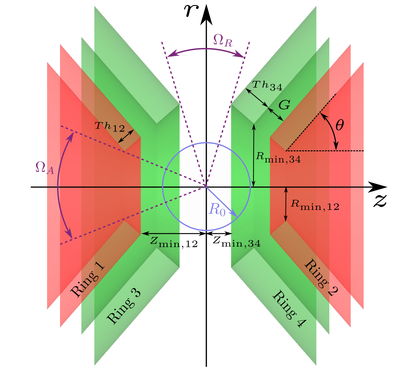
Figure 4: Definition of the geometric parameters used to optimise the trap: axial distance $Z_{min}$ from the radial axis to the closest point on a ring electrode, minimal radial distance $R_{min}$, radial thickness of the electrode $Th$, gap $G$ between two successive electrodes and cone angle $\theta$ from $z$-axis. $\Omega_{A}$ and $\Omega_{R}$ are respectively the axial and radial angular openings. The circle of radius $R_{0}$ used to compute the spherical harmonics is also drawn.

Some other parameters can be derived from these quantities like the gap $G$ between two electrodes, their outermost radii as well as the radial and axial angular acceptances respectively $\Omega_{R}$ and $\Omega_{A}$. These could help imposing some mechanical constrains in the minimisation procedure.

For some exploratory work, we had envisaged and tested more complicated shapes for the electrodes, including e.g. some splines to describe parts of their section, but the whole study showed that simpler shapes could suit our precision needs as we shall see in next section.

5 Optimisation process and results

Maximising the measured statistics with moratrap requires not only the trapping of as many ions as possible during a period as long as possible, but also a large angular aperture $\Omega_{R}$ in the radial direction where the $\beta$ and recoil ions detectors are located. In addition, the $D$ measurement relies on the knowledge of the ion cloud polarisation which shall be continuously monitored during the experiment Delahaye:2018 . This will be performed with two annular silicon detectors located along the trap $z$-axis before and after the electrodes. The central hole in these Si detectors lets the ion beam entering and exiting the trap. The axial angular acceptance of these detectors directly impacts the precision on the polarisation measurement and is constrained by the trap angular opening $\Omega_{A}$. All the above constrains have been taken care of in the optimisation process.

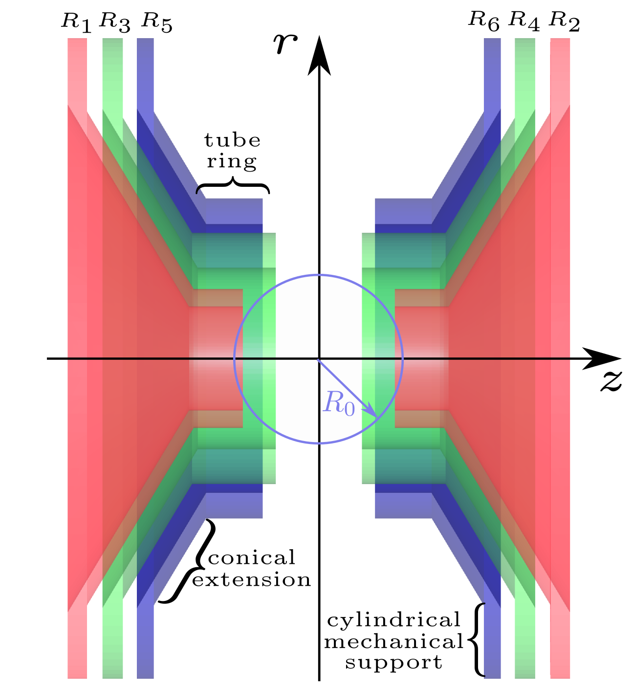
Figure 5: Cross section view of lpctrap geometry. There are three pairs of ring/tube electrodes with conical extensions and cylindrical mechanical support. $R_{1}$ and $R_{2}$ are the RF electrodes, $R_{3}$ and $R_{4}$ are used to inject and extract the ions and the external electrodes $R_{5}$ and $R_{6}$ are used to correct the potential generated along the $r$-axis and to steer the trajectories of the decay products. The circle of radius $R_{0}=10$ mm gives the overall scale.

A simplified version of lpctrap (Fig. 5) was used as a starting point to look for an optimal geometry as it already provides a large enough radial acceptance $\Omega_{R}$ Fabian:2014 . This starting geometry respects axial symmetry and also possesses a planar symmetry at $z=0$. However, on the contrary to lpctrap which uses three pairs of tube or cylinder shaped electrodes, in order to satisfy moratrap’s requirement of a larger axial acceptance $\Omega_{A}$, conical shapes were chosen for the two innermost pairs of electrodes. A third pair of electrodes ($R_{5}-R_{6}$) was added to screen the axially symmetric trap region from the octagonal set of detectors and associated collimators which might disturb the potential in the ROI (Fig. 1). This outermost set of electrodes is tube shaped, as in the lpctrap geometry. Two Einzel lens triplets, used to focus the incoming beam and to clean the trap after a measurement cycle, were also included in the simulation (Fig. 6). The shape of these lenses and of the outermost tube rings were optimised separately to fit some mechanical constrains and were kept fixed along the whole optimisation process of the two innermost electrode pairs. Because of their distance from the ROI they did not have any significant effect on the potential as will be seen in Sec. 7.

To ease later comparisons with lpctrap performances, it was decided to use, in the simulation, the same applied RF voltage of 60 V on the innermost pair of electrodes even if during moratrap operation we shall use 100 V or more (all other electrodes are grounded during the trapping period).

To summarise, the parameters related to outermost electrodes and Einzel lens triplets were already fixed prior to the whole minimisation process and we have chosen to optimise seven free parameters linked to the geometry of the internal and middle electrodes (Fig. 4): the axial distances $Z_{min,12}$ and $Z_{min,34}$, the radial distances $R_{min,12}$ and $R_{min,34}$, a common cone angle $\theta$ and the thicknesses $Th_{12}$ and $Th_{34}$. The minimisation of the objective function $f(\mathbf{a})$ (Eq. (16)) was performed within root-minuit Root:1997 ; James:1994 and to further reduce the parameter space to be explored, some lower positive limits were determined by exploratory simulations and set on the different distances $Z_{min}$ and $R_{min}$. The optimisation requires the computation of the potential harmonic spectrum. To this purpose, the convergence radius $R_{0}$ of the expansion was set to 10 mm which is about 5 times larger than the cloud radius observed with lpctrap. In addition, for the evaluation of $\rho_{2\%}$ from Eq. (15), we have chosen to truncate the expansion at $n_{\mathrm{max}}=18$, as the contribution from the $A_{18}$ term, belonging to the quadrupole series, is already very small. Indeed the absolute difference between the potential computed in electrobem and the potential synthesised from harmonics up to order 18 is smaller than 2.5$\times 10^{-7}$ V for the 64800 points used to compute the harmonics while the potential at these points varies from 15 to 37 V.

		Rings
Parameter	$\bm{R_{1}/R_{2}}$	$\bm{R_{3}/R_{4}}$	$\bm{R_{5}/R_{6}}$
$\theta$ (∘)	49	49	0
$Z_{\mbox{\scriptsize{min}}}$ (mm)	13.41	6.00	13.00
Thickness (mm)	2.50	4.53	4.50
Inner radius (mm)	8.03	15.56	39.29
Outer radius (mm)	9.67	18.53	43.79

Table 1: Optimised moratrap electrodes dimensions.

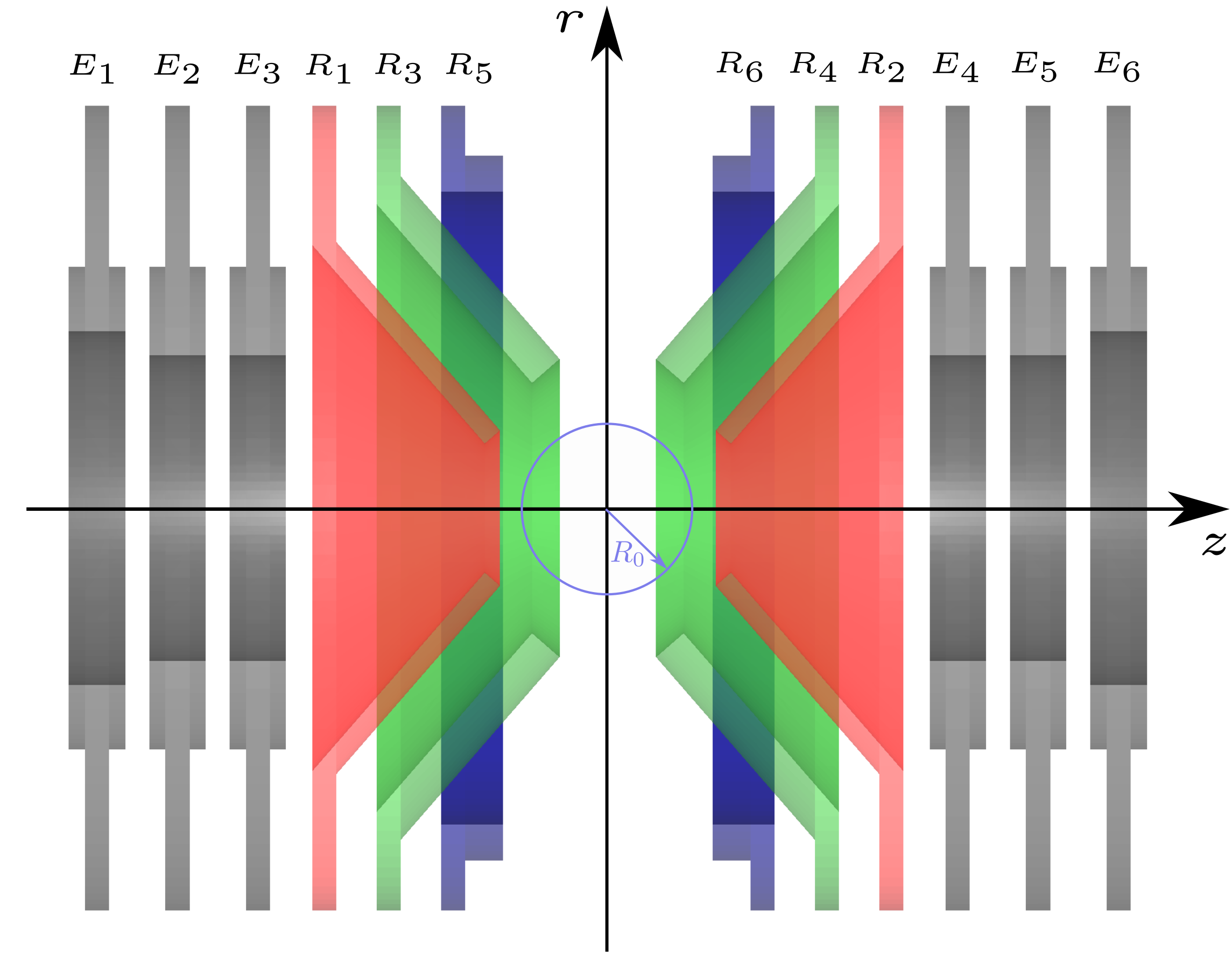
Figure 6: Cross section view of the optimised moratrap geometry. A RF voltage is applied to the innermost ring pair ($R_{1}$, $R_{2}$), while the middle and outer electrodes, as well as the Einzel lenses are grounded. $z$-axis is along the beam injection and extraction. The geometry is symmetric with respect to the $x-y$ plane and is invariant around the $z$ axis. The circle of radius $R_{0}=10$ mm gives the overall scale, but more precise dimensions are given in Table 1.

After several iterations, minuit converged to a minimum of the objective function at $\rho_{2\%}=7.39$ mm. The optimised geometric parameters of the electrodes corresponding to this $\rho_{2\%}$ are presented in Table 1 and a cross section view of moratrap is shown in Fig. 6. The precision on distances is limited to the machining tolerance ($10\text{\,}\mathrm{\SIUnitSymbolMicro m}$). Effects of this limited precision are studied in Sec. 7. The radial angular acceptance $\Omega_{R}$, as seen from the trap centre, is $35.9^{\circ}$. It is limited by the axial position of rings $R_{3}$ and $R_{4}$. The axial angular acceptance $\Omega_{A}$ is $55.4^{\circ}$ and is limited by the inner radius of ring $R_{1}$ or $R_{2}$. This acceptance is large enough to install the two annular detectors (with a hole radius of 6 mm) before and after the Einzel lens triplets at 70 mm from the trap centre Delahaye:2018 .

The harmonic coefficients $A_{n}$ ($n\in[0,18]$) of the potential, computed at $\rho_{2\%}$, are presented in Fig. 7. The ratios $\frac{A_{4}}{A_{2}}$, $\frac{A_{6}}{A_{2}}$ and $\frac{A_{8}}{A_{2}}$ are respectively around $-3.2\times 10^{-7},\,-1.9\times 10^{-2}$ and $-3.3\times 10^{-4}$, they confirm the dominance of the quadrupole term ${A_{2}}$. Top panel in Fig. 8 shows the potential (without the constant term $n=0$) in the trapping region of moratrap for $\rho\leqslant\rho_{2\%}$. Middle and bottom panels demonstrate how small the contribution of these higher multipoles ($n>2$) is. Since the octupole term $A_{4}$ is of the order of $10^{-6}$, the largest contribution comes from the dodecapole term $A_{6}$. Bottom panel of Fig. 8 presents in more details the contribution from harmonics with orders greater or equal to 8: they are even lowered by about a factor 10 to 100 depending on the angular position. These results demonstrate that the minimisation procedure led to a quadrupole potential with the required quality, a relative difference to $A_{2}$ lower than 2% (see Eq. (15)), in a region with a radius as large as 7.39 mm.

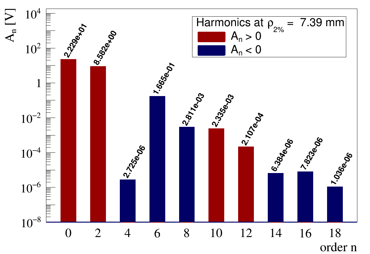
Figure 7: Harmonics coefficients for moratrap up to order 18, extracted from potential sampled on a circle of radius $\rho_{2\%}=7.39$ mm using axielectrobem, when applying 60 V on the innermost electrodes and 0 V on all the other electrodes. Positive and negative harmonics have been separated in order to display them with logarithmic scale.

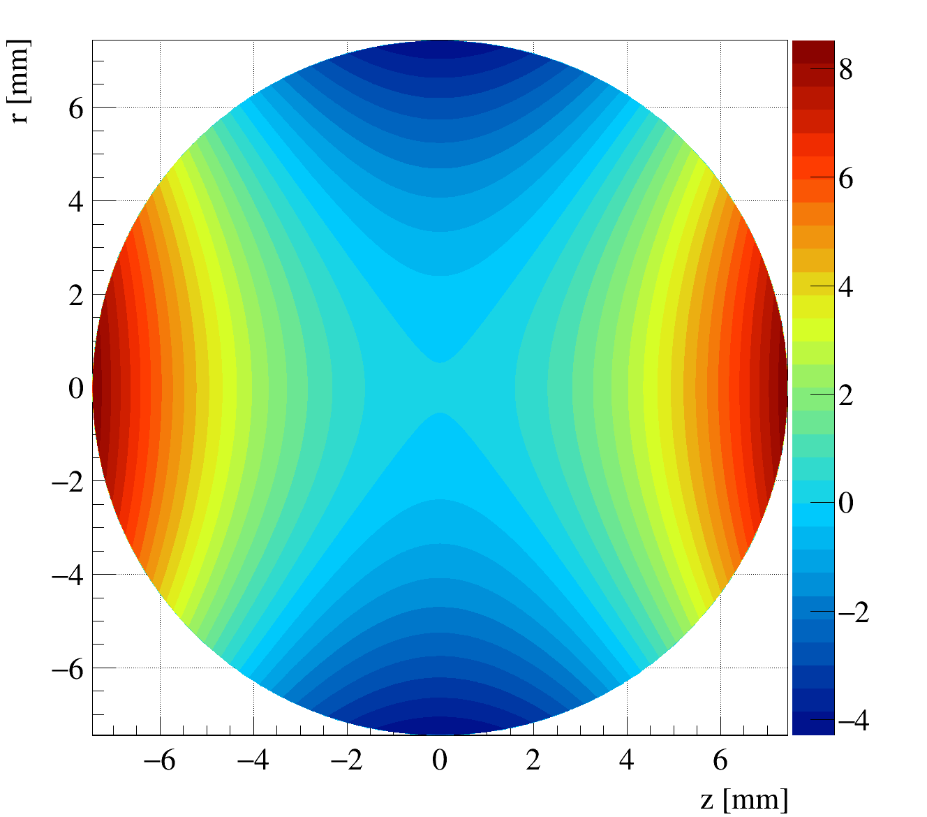
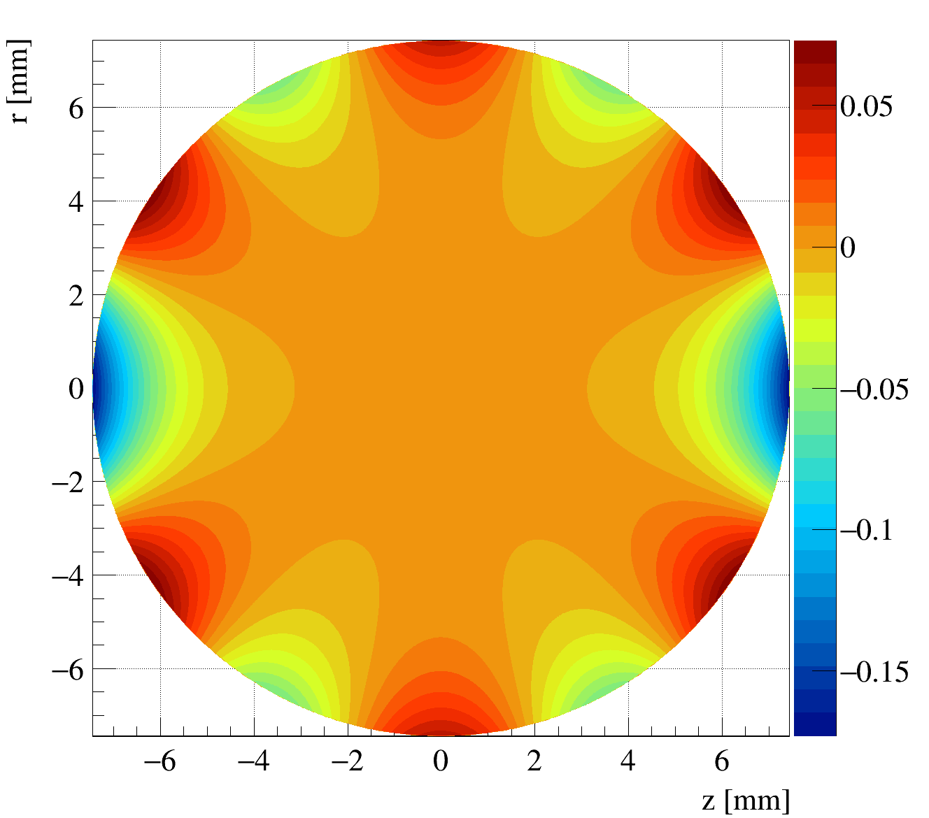
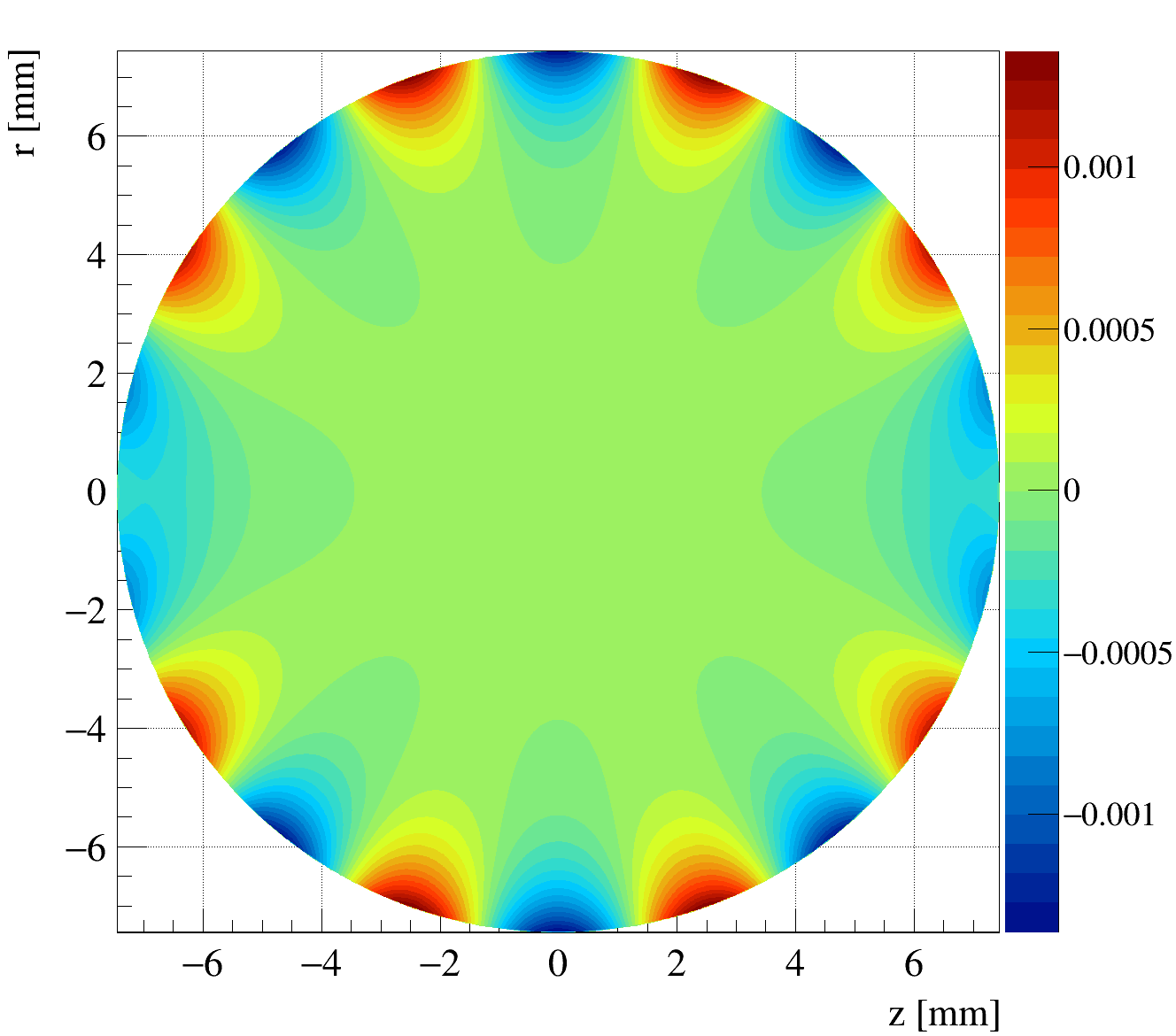
Figure 8: Contribution to the potential for $\rho\leqslant 7.39$ mm in moratrap from different harmonics sets (vertical scale is in volts). Top panel corresponds to harmonics with $n\geqslant 2$ and exhibits a strong quadrupole dependence. Middle panel is for $n\geqslant 4$ and clearly shows the dodecapole contribution. Bottom picture shows the contribution from all harmonics with $n\geqslant 8$.

In next section we shall compare these performances to those of lpctrap.

6 Comparison of MORATrap and LPCTrap

It is interesting to compare moratrap performances with those of lpctrap. For this purpose, the potential generated in lpctrap (Fig. 5) was simulated in axielectrobem and the harmonics were determined as seen in Fig. 9, where obviously the octupole term is much larger than in moratrap. One should however notice that $A_{4}$ and $A_{6}$ have opposite signs, thus partly compensating each others in the low radii region before $A_{6}$ takes over at larger radii. The ratios $\frac{A_{4}}{A_{2}}$, $\frac{A_{6}}{A_{2}}$ and $\frac{A_{8}}{A_{2}}$ are respectively around $+5.5\times 10^{-3},\,-1.4\times 10^{-2}$ and $+9.0\times 10^{-5}$. The corresponding radius $\rho_{2\%}$ is equal to 4.36 mm which is about 40% smaller than for moratrap. This clearly demonstrates that we have succeeded to broaden the trapping region in moratrap and to improve the potential quality compared to lpctrap, given some maximal constraints in dimension for the Paul trap. In addition, due to its tube-shape electrodes, lpctrap has an axial angular aperture of $43.6^{\circ}$ whereas for moratrap $\Omega_{A}=55.4^{\circ}$, i.e. 27% larger. The radial angular acceptances $\Omega_{R}$ are similar in both traps, respectively $38.0^{\circ}$ and $35.9^{\circ}$ with a small advantage of 6% for lpctrap. However, it is important to emphasise that in a trap, the amount of particles which can be effectively trapped is directly proportional to the depth of the potential well i.e. the value of $A_{2}$ and to the r adius $\rho_{2\%}$ (Eq. (6)). One can note that in moratrap, at $\rho=4.36$ mm, to reach the same value of the quadrupole term as in lpctrap, would require to apply 138 V instead of 60 V like in the simulations presented throughout this paper.

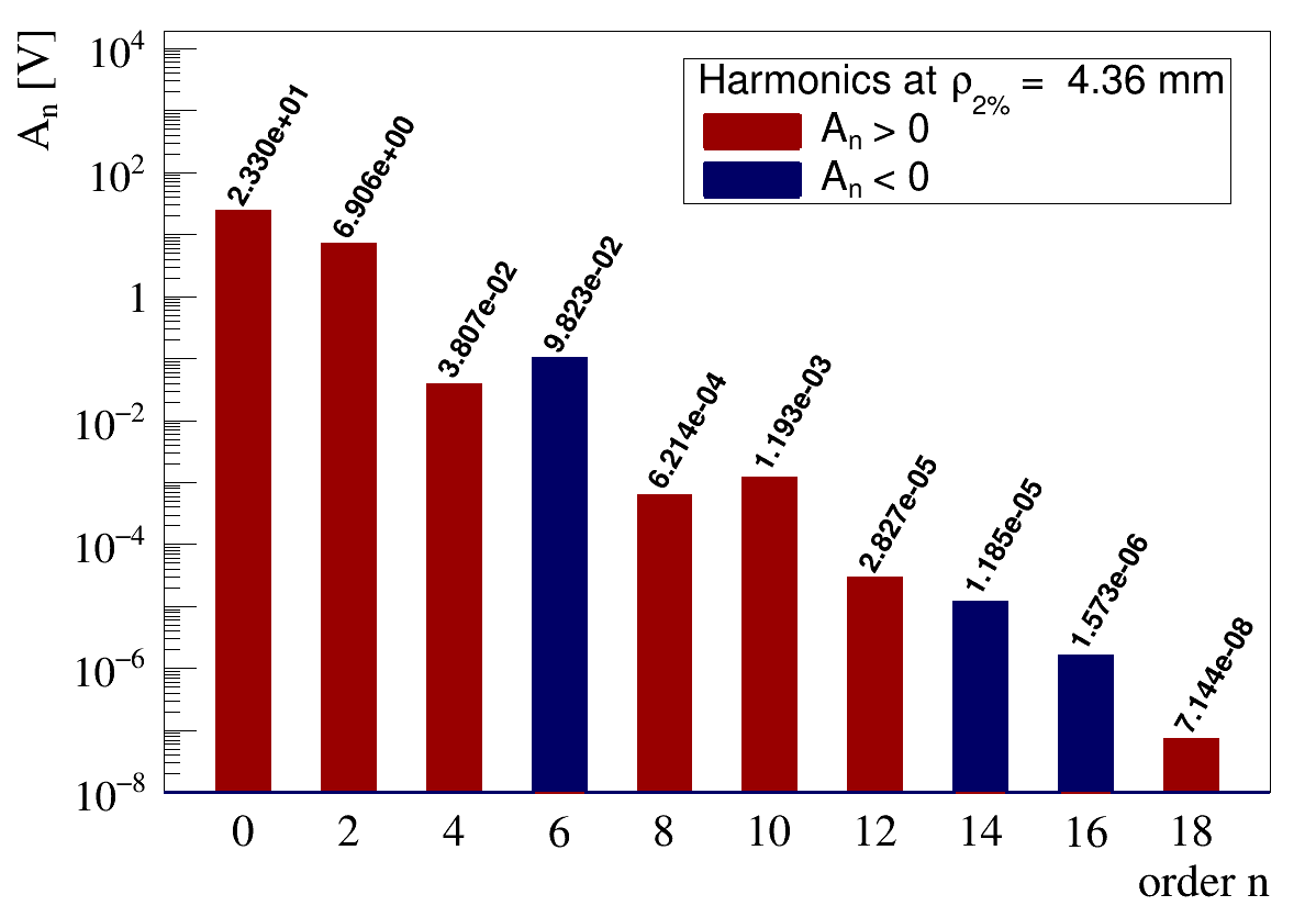
Figure 9: Harmonics coefficients for lpctrap up to order 18, extracted from potential sampled on a circle of radius $\rho_{2\%}=4.36$ mm using axielectrobem, when applying a 60 V RF voltage on the innermost electrodes.

To deepen this comparison it is interesting to make a parallel with an ideal Paul trap, introduced in Sec. 1. For real Paul traps, one can define an equivalent internal radius $r_{0}$ as defined for ideal Paul traps in Eq. (1), representing the radius at which the RF voltage would be applied to yield the same $A_{2}$ value at a given $\rho_{2\%}$:

$$r_{0}^{2}\,=\,\rho^{2}_{2\%}\,\frac{V_{0}}{A_{2}}.$$ (17)

Compared to an ideal Paul Trap, moratrap has an effective internal radius $r_{0}$ significantly larger than the one of lpctrap which explains the relative difference in $A_{2}$ values at a given radius for both traps. From the $A_{2}$, $\rho_{2\%}$ and $V_{0}$ values shown in Figs.7 and 9, one finds an effective internal radius of 19.24 mm for moratrap, and of 12.86 mm for lpctrap. This is consistent with what was found in Delahaye:2019 and is summarised in Table 2. It is important however to note that simply scaling lpctrap to the same internal radius as moratrap would not have yielded the same improvements: the 2% radius would have been enlarged to only 6.53 mm, compared to 7.39 mm in the case of moratrap, and the axial angular acceptance $\Omega_{A}$ would still have been limited by 27% compared to moratrap. The trap capacity of moratrap, estimated thanks to Eq. (6) and considering $r_{\mathrm{eff}}\,\simeq\,\rho_{2\%}$, has been enlarged by more than a factor of 2 compared to the original lpctrap, and by 40% compared to a scaled version of lpctrap.

	lpctrap	moratrap	lpctrap
			scaled
$V_{0}$ [V]	60	60	60
$r_{0}$ [mm]	12.86	19.24	19.24
$\rho_{2\%}$ [mm]	4.36	7.39	6.53
$A_{2}(\rho_{2\%})$ [V]	6.91	8.58	6.91
$\rho_{2\%}A_{2}$ [V.mm]	30.14	63.44	45.09
Maximum capacity	$1.05\text{\times}{10}^{6}$	$2.20\text{\times}{10}^{6}$	$1.56\text{\times}{10}^{6}$

Table 2: Comparison of moratrap and lpctrap when both traps are assumed to behave like ideal Paul traps exhibiting a pure quadrupole potential. The maximum capacity was estimated for a pseudo potential model with a Mathieu parameter $q_{z}=0.4$ and for singly charged positive ions. After rescaling lpctrap effective internal radius to the $r_{0}$ of moratrap, its radius $\rho_{2\%}$ is still smaller than the one obtained for moratrap and its maximum capacity is about 30% smaller.

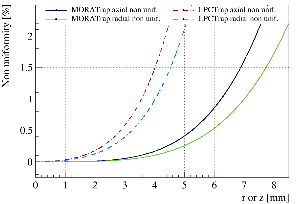
Figure 10: Radial and axial non uniformities, respectively given by Eq. (18) and Eq. (19), as a function of the radial and axial distance from moratrap centre.

To further compare both traps, one can investigate the potential non uniformity as a function of the space coordinates. We can for instance define a radial and an axial non uniformity respectively by:

$$U_{\mathrm{Radial}}(r) = \sum_{n=4}^{18}\left(\frac{r}{R_{0}}\right)^{\!\!n-2}\left|\frac{A_{n}P_{n}(0)}{A_{2}P_{2}(0)}\right|\,\,\,\,\mathrm{at}\,\,\,\,z=0,$$ (18)

$$U_{\mathrm{Axial}}(z) = \sum_{n=4}^{18}\left(\frac{z}{R_{0}}\right)^{\!\!n-2}\left|\frac{A_{n}}{A_{2}}\right|\,\,\,\,\mathrm{at}\,\,\,\,r=0,$$ (19)

where the Legendre polynomial $P_{n}(\cos\theta)$ present in Eq. (12) is equal to unity along $z$-axis and to $P_{n}(0)$ along $r$-axis. These quantities are presented in Fig. 10 where, in agreement with the values of $\rho_{2\%}$ found previously, the region where the radial and axial non uniformities are very weak is wider in the case of moratrap.

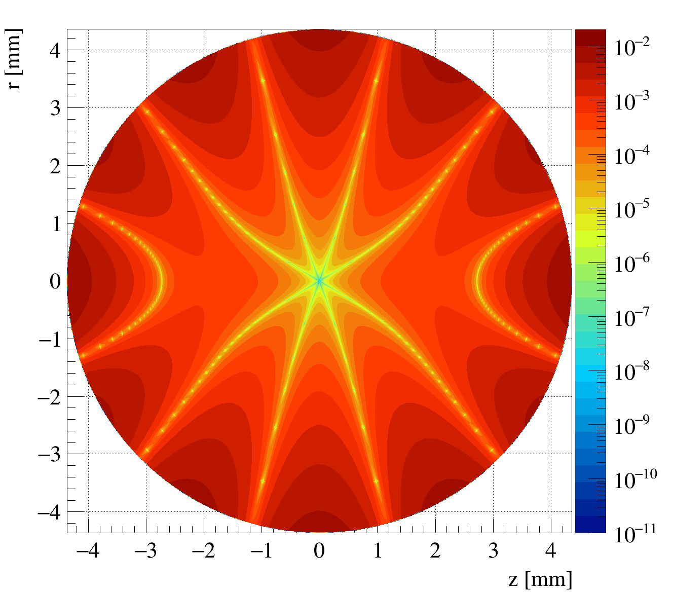
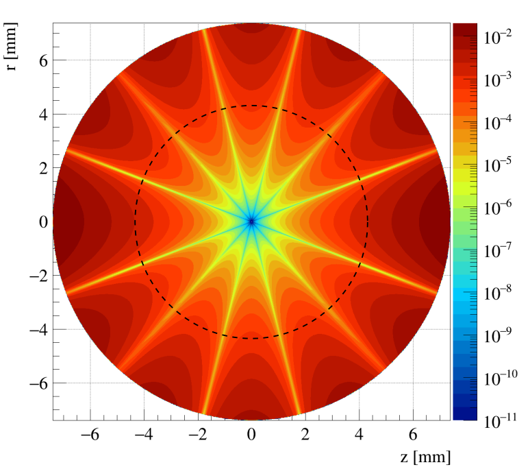
Figure 11: Top: Potential non uniformity obtained with Eq. (20), for lpctrap region of interest, i.e. for $\rho=\sqrt{r^{2}+z^{2}}\leqslant\rho_{2\%}=4.36$ mm. Bottom: Same figure for moratrap with $\rho_{2\%}=7.39$ mm. The dashed black circle corresponds to the lpctrap 2% radius.

Another way to visualise the difference between the two traps is to draw a 2D uniformity defined as:

$$U(r,z)=\left|\sum_{n=4}^{18}\left(\frac{r}{R_{0}}\right)^{\!\!n-2}\frac{A_{n}}{A_{2}}\,P_{n}(\cos\theta)\right|.$$ (20)

where the absolute value has been chosen such that a logarithmic scale may be used to help distinguishing more details. Figure 11 shows $U(r,z)$ for $\rho\leqslant 4.36$ mm in the case of lpctrap (top panel) and $\rho\leqslant 7.39$ mm in the case of moratrap (bottom panel). The dashed black circle on bottom panel represents the limit of the region where the potential non uniformity is smaller than 2% in lpctrap.

All these different definitions of the non uniformity conclude to the improvement of the potential quality and of the trapping region volume in moratrap compared to lpctrap.

In next section, we shall investigate how stable is the potential against misalignment and other mechanical characteristics.

7 Design sensitivity

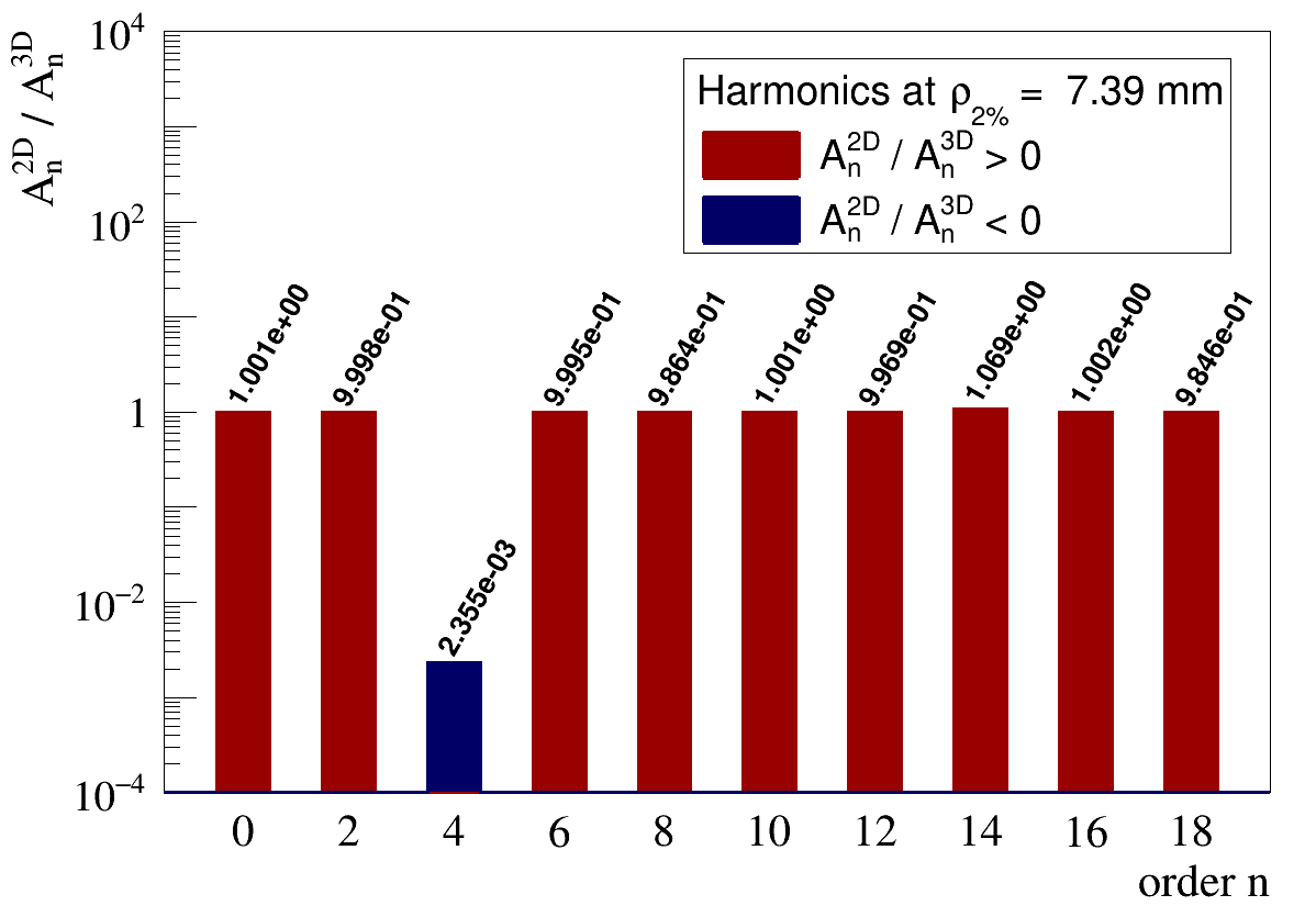
Figure 12: Comparison between harmonics computed with axielectrobem and electrobem with an angular/polygonal segmentation of 84 cells around $z$-axis. Except for $A_{4}$, all harmonics are equal to better than a few percents, especially for low order ones.

It is important to check how the mechanical tolerances in the machining and assembling of the different electrodes of moratrap can affect the trapping potential. For this purpose, the effects on the potential due to mechanical precision, in terms of machining defects or misalignment of one or several electrodes, were investigated using both axielectrobem (2D) and electrobem (3D). axielectrobem was preferred in case of defects not breaking axisymmetry, whereas electrobem was used in other cases. When performing simulations within electrobem, the setup needs to be meshed not only in the axial direction, but also angularly around this axis: a circle is approximated by a polygon and thus any cone, disk or cylinder is segmented in many triangular or quadrangular cells. As mentioned in Sec. 2, the computer RAM usage rapidly increases when working in 3D compared to axially symmetric simulations. On the computer used, the available RAM allowed us to divide the setup in 84 cells in angle while keeping the same axial segmentation as the one used in axielectrobem leading to 84 $\times$ 414 = 34776 cells in total. Such a meshing has consequences on the computed harmonics spectrum. Figure 12 shows the ratio of the harmonics from the 2D axisymmetric case to the 3D one. There is a very good agreement between the two: it is better than a few percents except for the octupole term $A_{4}$, which appears to be very sensitive to the angular discretisation and dramatically changes not only in absolute value, but also in sign. Nevertheless, the 3D computation leads to a value of $A_{4}$ still about a factor 100 less than $A_{6}$ and its contribution to the potential is therefore very limited. When using 3 planes of symmetry in electrobem, one can simulate 1/8 of moratrap with as many cells as a full simulation without symmetry planes. In that case, the 3D harmonics spectrum agrees with the 2D one within a few $10^{-6}-10^{-5}$ even for $A_{4}$. However, most of the envisaged defects break at least one of these symmetries. Consequently, the full moratrap has to be simulated in these studies and the results should be compared to those from the perfectly aligned 3D version of moratrap rather than to those from axielectrobem. The precision on the evaluated potential essentially depends on the characteristics of the electrode mesh and is constant once this mesh has been fixed. A single mesh is used to test different trap configurations with or without misalignment. The results obtained for configurations exhibiting some defects are compared to a reference one where the electrodes are perfectly aligned and machined (in the limit of the mesh discretisation) and therefore one expects that the observed differences are highly significant overall.

The considered defects included machining tolerances of $\delta r$ and $\delta z\leqslant$20\text{\,}\mathrm{\SIUnitSymbolMicro m}$$, axial and radial translations of $\Delta x$ and $\Delta z\leqslant$200\text{\,}\mathrm{\SIUnitSymbolMicro m}$$ and rotations around $r$-axis of $\Delta\theta\leqslant\leavevmode\nobreak\ 0.2^{\circ}$. All these values are larger than what can be mechanically achieved for moratrap. These defects were simulated for either one half of the trap in a whole or for electrodes taken individually while keeping the rest of the trap unchanged.

When dealing with individual electrodes, because of their relatively large distance from the trap ROI, all types of defects related to $R_{6},E_{4},E_{5}$ and $E_{6}$ have been shown to have very minor influence on the harmonics spectrum and therefore on the potential quality. This was also the case for possible machining defects on $R_{1},R_{2},R_{3}$ and $R_{4}$ as the computer numerical control machining precision was assumed better than $20\text{\,}\mathrm{\SIUnitSymbolMicro m}$.

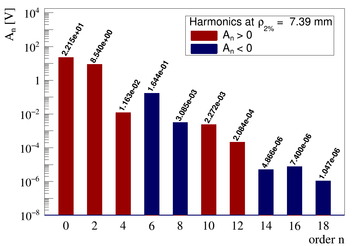
Figure 13: Harmonics spectrum obtained when translating left half of moratrap by $\Delta z=-$100\text{\,}\mathrm{\SIUnitSymbolMicro m}$$. The expansion has been computed around a centre located at half of the displacement ($z=-$50\text{\,}\mathrm{\SIUnitSymbolMicro m}$$) where the translated potential centre stands, i.e. where the ion cloud barycentre will be.

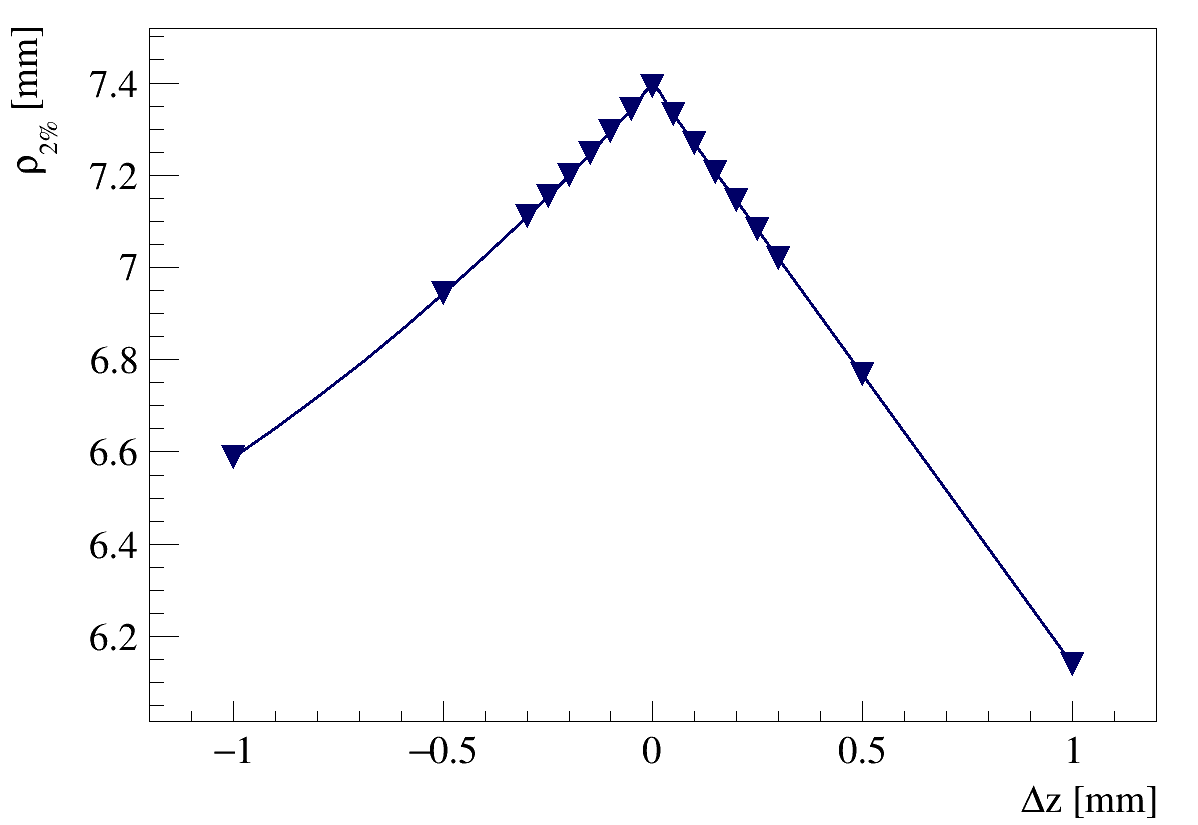
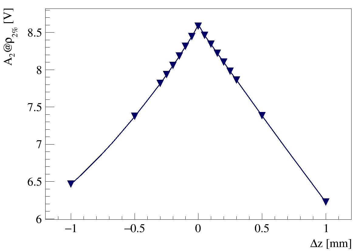
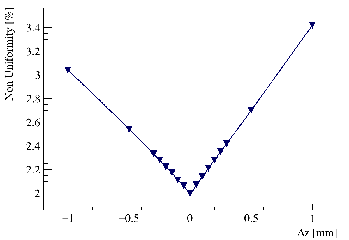
Figure 14: Evolution of the radius $\rho_{2\%}$, the quadrupole term $A_{2}\,\mathrm{at}\,\rho_{2\%}$ and the uniformity as a function of $\Delta z$, the translation distance of the left half of the trap (at $z<0$) from its nominal position. These results were obtained using axielectrobem.

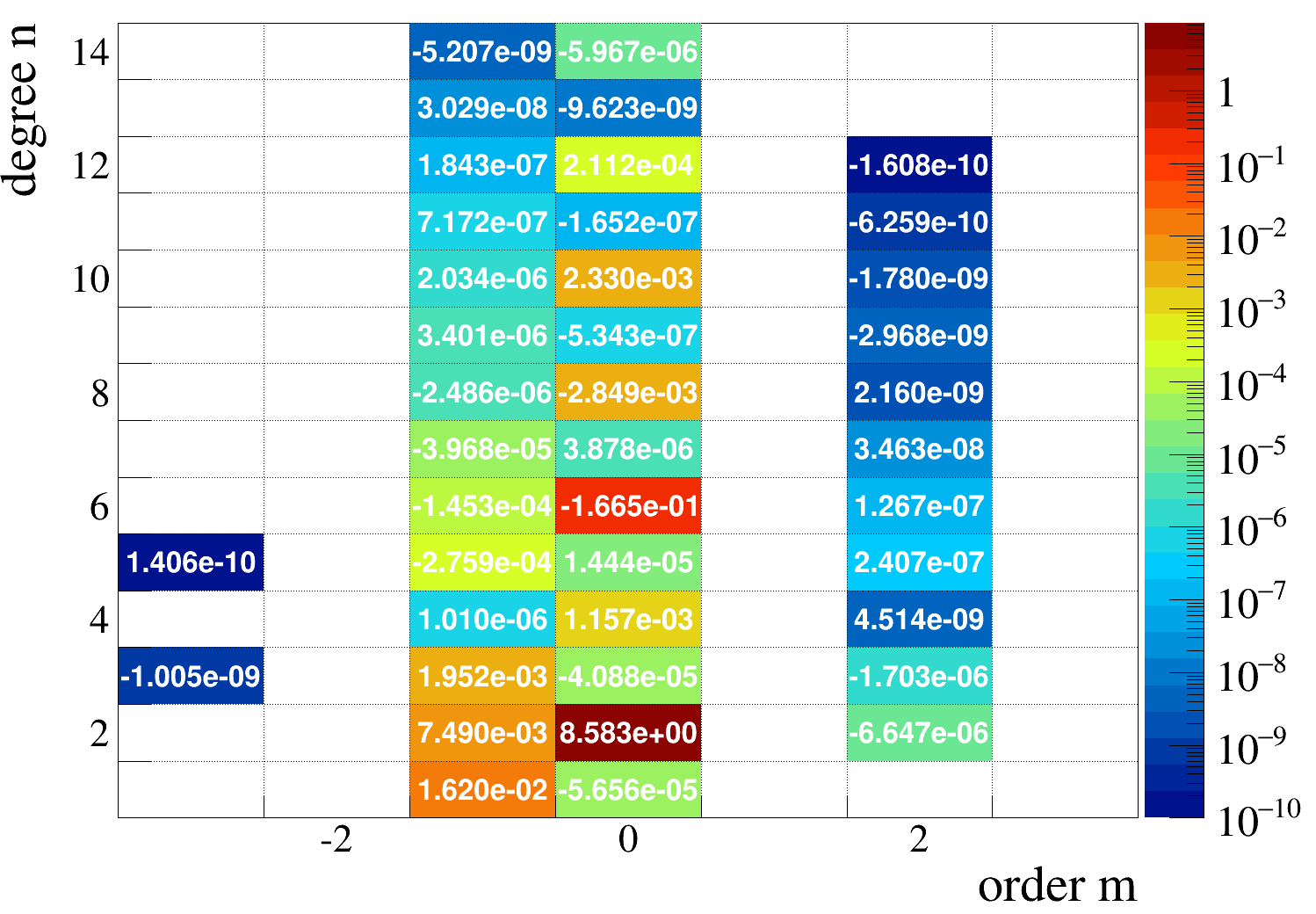
Figure 15: Harmonics spectrum (without the constant term $A_{0,0}$) obtained at $\rho_{2\%}$ with electrobem for half of the trap rotated by $0.2^{\circ}$ around $x$-axis (vertical scale is in volts). The series expansion centre is kept at the frame origin which does not correspond to the minimum of the potential after rotation. Harmonics with absolute values below $10^{-10}$ have been set to zero as their contribution to the potential is completely negligible.

The influence of misalignment along the $z$ direction was studied with axielectrobem by varying electrode(s) axial position. An axial displacement $\Delta z$ of half of the trap conserves both the axisymmetry and the planar symmetry: such a displacement shifts the trap centre by $\Delta z/2$ and therefore the potential still exhibits a planar symmetry around the position of this shifted centre. The potential harmonics expansion should therefore be determined around this shifted centre to avoid inducing spurious harmonics with odd orders. In the particular case of ion traps, the ion cloud barycentre will follow the potential centre and, in case of a large shift, this may modify the acceptance and have some consequences both on the detector counting rates and on the measured $\beta$ decay asymmetry. This shall be addressed in other simulations. Figure 13 presents the harmonics spectrum computed around a point located at $z=\Delta z/2=-$50\text{\,}\mathrm{\SIUnitSymbolMicro m}$$ for a global translation of all electrodes located at negative $z$ by $\Delta z=-$100\text{\,}\mathrm{\SIUnitSymbolMicro m}$$. One clearly sees that odd harmonics are not present in this spectrum. In this case, the potential quality is still suitable to trap ions as may be seen in Fig. 14 which shows the evolution of $\rho_{2\%}$, $A_{2}$ and the non uniformity (Eq. (15)) versus the translation $\Delta z$. A non uniformity of 2.5% is reached for displacements as large as 0.4 mm and even for such large $\Delta z$, $\rho_{2\%}$ is still about 6.9 mm and $A_{2}$ is only lowered by less than 10%.

To describe and further compare the harmonics induced by all the studied translations and rotations of different setup parts, we shall use the spherical harmonics with degree $n$ and order $m$ (Eq. (11)) instead of the cylindrical harmonics of order $n$ (Eq. (12)) used so far. Indeed, breaking the axisymmetry and/or the planar symmetry may induce some harmonics with different degrees $n$ but also and above all with non zero order $m$ on the contrary to what has been seen previously. As an example, Fig. 15 shows the harmonics corresponding to a setup where half of the trap has been rotated by $\Delta\theta=0.2^{\circ}$ around $x$-axis. One should notice that even if the potential centre has probably been shifted away from the reference frame origin, the harmonics expansion is still performed around this origin. The largest harmonics generated by the rotation are however a factor 10 smaller than the main ones and should therefore weakly impact the quality of the trapping potential. To estimate their influence and similarly to what was done in Eqs. (15), (18) and (19), we shall define a 3D non uniformity. This is more difficult as the associated Legendre functions of the first kind $P_{n}^{m}(\cos\theta)$ are not bounded to $[-1,1]$ on the contrary to the Legendre polynomials $P_{n}(\cos\theta)$: their minimum (resp. maximum) values strongly decrease (resp. increase) with degree $n$ and order $m$. However they always satisfy $\max(P_{n}^{m}(x))\geqslant|\min(P_{n}^{m}(x))|$. This inspired us to define a 3D non uniformity at $\rho=R_{0}=\rho_{2\%}$ (maximising the radial contribution) by:

$$U_{\mathrm{3D}}\,=\,\sum_{n=1}^{n_{\mathrm{max}}}\sum_{\begin{subarray}{c}m=0\,\mathrm{if}\,n\neq 2\\ m=1\,\mathrm{if}\,n=2\end{subarray}}^{n}\!\max(P_{n}^{m}(\cos\theta))\frac{|A_{nm}|\,+\,|B_{nm}|}{|A_{2,0}|},$$ (21)

where the numerator and therefore $U_{\mathrm{3D}}$ have been maximised by setting the functions $P_{n}^{m}(\cos\theta)$, $\cos(m\varphi)$ and $\sin(m\varphi)$ to their maximal values and by taking the absolute values of the harmonic coefficients. For the denominator we only keep $|A_{2,0}|$ without any spatial dependent function which might become null at some location leading to an infinite value of $U_{\mathrm{3D}}$. When simulating moratrap in electrobem without any misalignment, the 3D non uniformity $U_{\mathrm{3D}}$ is 2.017 %, which shall serve as our reference. One should notice that this value is weakly above the 2% limit obtained with axielectrobem, this highlights the influence of the 3D meshing. The $U_{\mathrm{3D}}$ values obtained for the tested misalignment are presented in Tables 3 and 4 respectively for translations ($\Delta z$, $\Delta x$) and rotations ($\Delta\theta$). These clearly demonstrate that displacements of either rings $R_{5}$ and $R_{6}$ or Einzel lens triplets have negligible influence on the potential quality within the ROI. The largest non uniformities are obtained for translations $\Delta x$ of ring electrode $R_{4}$ or for the rotation of half of the trap. Even if these non uniformities were extracted from harmonics series expansions performed around the reference frame origin instead of around the potential centre, they still remain smaller than 2.5%, i.e. at a level sufficient to maintain the trapping efficiency Delahaye:2019 .

Translated	$\mathbf{\Delta z}$	$\mathbf{U_{3D}}$	$\mathbf{\Delta x}$	$\mathbf{U_{3D}}$
part	[$\text{\,}\mathrm{\SIUnitSymbolMicro m}$]	[%]	[$\text{\,}\mathrm{\SIUnitSymbolMicro m}$]	[%]
Half trap	100	2.127	200	2.398
$R_{2}$	100	2.182	200	2.208
$R_{4}$	100	2.142	200	2.461
$R_{6}$	100	2.017	200	2.017
$E_{4}$	100	2.017	200	2.017
$E_{5}$	100	2.017	200	2.017
$E_{6}$	100	2.017	200	2.017

Table 3: 3D non uniformity due to $\Delta z$ and $\Delta x$ misalignment of the half trap and of individual electrodes.

Rotated	$\mathbf{\Delta}\bm{\theta}$	$\mathbf{U_{3D}}$
part	[∘]	[%]
Half trap	0.2	2.404
$R_{2}$	0.2	2.267
$R_{4}$	0.2	2.159
$R_{6}$	0.2	2.018
$E_{4}$	0.2	2.017
$E_{5}$	0.2	2.017
$E_{6}$	0.2	2.017

Table 4: 3D non uniformity due to $\Delta\theta$ misalignment. Here the series expansion centre is kept at the frame origin. Realistic mechanical rotations of at most 0.2^∘ lead to non uniformities well below 2.5%.

All the reasonable mechanical defects studied have been shown to weakly affect the quality of the potential and the volume of the trapping region in moratrap if the machining process and the alignment of the different electrodes during assembly are kept under control. It was therefore decided to design, machine and assemble the moratrap electrodes at LPC Caen. A picture of this realisation is shown in Fig. 16.

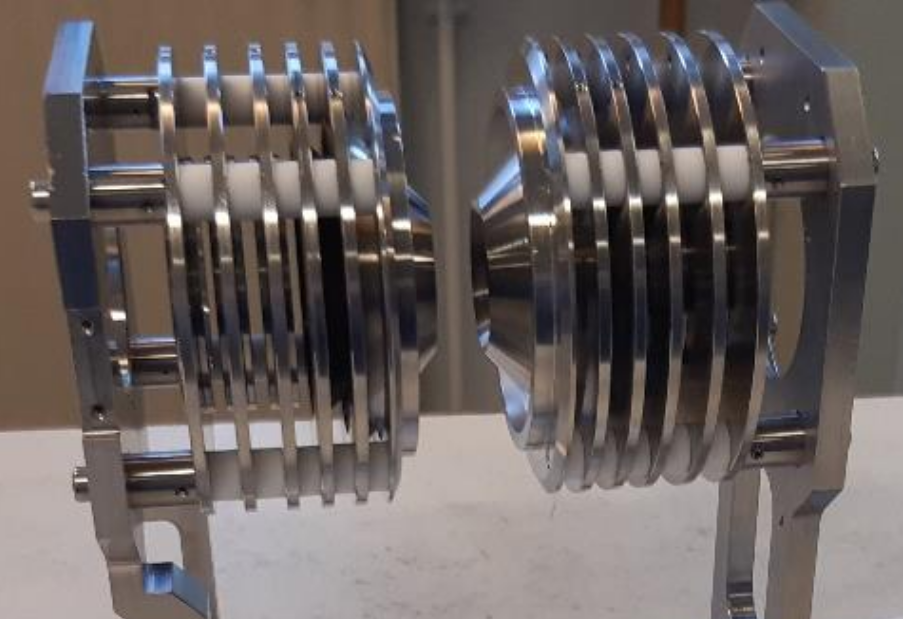
Figure 16: Picture of moratrap on its mechanical support. It has been machined and assembled at LPC Caen.

8 Conclusion

We have presented a method used to optimise the geometry of the axially symmetric ion trap, moratrap, dedicated to the measurement of the triple correlation parameter $D$ in nuclear $\beta$-decay of radioactive ions. Our starting point was the lpctrap geometry, the former used transparent Paul trap, and we succeeded in reducing the contribution to the potential from harmonics of order higher than 2. This is necessary to achieve a longer storage time and a better trapping efficiency. According to the pseudo-potential approximation, the moratrap capacity has been enlarged by more than a factor of 2 compared to the initial lpctrap geometry. The optimised geometry exhibits a larger axial angular acceptance than in lpctrap. This larger acceptance is necessary for the online monitoring of the trapped ion cloud polarisation, by detecting $\beta$ particles along the axis of the trap. Further simulations are currently being performed to deeply investigate the ion cloud dynamics, the trapping efficiency as well as the trapping time. The optimised trap electrodes could easily be machined with a mechanical precision of the order of $10\text{\,}\mathrm{\SIUnitSymbolMicro m}$. The whole setup should be soon tested and then installed at JYFL accelerator facility in University of Jyväskylä (Finland) before its final operation at GANIL - DESIR (Caen, France).

The optimisation method described in this study could easily be applied to other axisymmetric ion traps or electrodes setups. Different types of fitness functions could bring many improvements to the method and should be explored in detail.

Appendix A Homogeneous polynomials in cylindrical axisymmetric coordinates

For completeness, in this appendix, we present a series expansion for the potential of an axisymmetric system in cylindrical coordinates $(r,z)$. Starting from the coordinates conversion relations $\rho^{2}=r^{2}+z^{2}$ and $\cos\theta=z/\rho$ and introducing the homogeneous harmonic polynomials $H_{n}(r,z)$ given by an explicit relation rather than by a recurrence one:

$$H_{n}(r,z) = \rho^{n}\,P_{n}(\cos\theta)$$ (22)

$$= \sum_{k=0}^{E[n/2]}\,\frac{n!}{(-4)^{k}(n-2k)!(k!)^{2}}\,r^{2k}\,z^{n-2k},$$

the potential given by Eq. (12) is rewritten as :

$$V(r,z)\,=\,\sum_{n=0}^{\infty}\,\frac{A_{n}}{\rho_{0}^{n}}\,H_{n}(r,z).$$ (23)

This series expansion converges for points $(r,z)$ satisfying $\sqrt{r^{2}+z^{2}}\leqslant\rho_{0}$ with $\rho_{0}$ the convergence radius. Again, a planar symmetry at $z=0$ allows to further reduce the multipole expansion to even harmonics only. The first harmonic polynomials are listed up to order 10 in Table 5.

$\mathbf{n}$	$\mathbf{H_{n}(r,z)}$
0	$1$
1	$z$
2	$\frac{1}{2}\left(2z^{2}-r^{2}\right)$
3	$\frac{1}{2}\left(2z^{3}-3r^{2}z\right)$
4	$\frac{1}{8}\left(3r^{4}-24z^{2}r^{2}+8z^{4}\right)$
5	$\frac{1}{8}\left(8z^{5}-40r^{2}z^{3}+15r^{4}z\right)$
6	$\frac{1}{16}\left(-5r^{6}+90z^{2}r^{4}-120z^{4}r^{2}+16z^{6}\right)$
7	$\frac{1}{16}\left(16z^{7}-168r^{2}z^{5}+210r^{4}z^{3}-35r^{6}z\right)$
8	$\frac{1}{128}\left(35r^{8}-1120z^{2}r^{6}+3360z^{4}r^{4}-1792z^{6}r^{2}+128z^{8}\right)$
9	$\frac{1}{128}\left(128z^{9}-2304r^{2}z^{7}+6048r^{4}z^{5}-3360r^{6}z^{3}\right.$
	$\qquad\left.+315r^{8}z\right)$
10	$\frac{1}{256}\left(-63r^{10}+3150z^{2}r^{8}-16800z^{4}r^{6}+20160z^{6}r^{4}\right.$
	$\qquad\left.-5760z^{8}r^{2}+256z^{10}\right)$

Table 5: Harmonic polynomials of degree $n\leqslant 10$ in axisymmetric cylindrical coordinates $(r,z)$.

References

- [1] M. Gonzáles-Alonzo et al. New physics searches in nuclear and neutron decay. Progr. in Part. and Nucl. Phys, 104:165, 2019.
- [2] A. Sakharov. Violation of CP invariance, C asymmetry, and baryon asymmetry of the universe. JETP Letters, 5:24–27, 1967.
- [3] P. Delahaye et al. The MORA project. Hyperfine Interact., 240(1):63, 2019.
- [4] M.G. Sternberg et al. Limit on Tensor Currents from 8Li Decay. Phys. Rev. Lett., 115:182501, 2015.
- [5] M. Brodeur et al. Vud determination from light nuclide mirror transitions. Nucl. Intr. Meth., B376:281, 2016.
- [6] G. Ban et al. Precision measurements in nuclear -decay with LPCTrap. Annalen Phys., 525(8-9):576–587, 2013.
- [7] X. Fabian et al. Precise measurement of the angular correlation parameter in the decay of 35Ar with LPCTrap. EPJ Web Conf., 66:08002, 2014.
- [8] E. Liénard et al. Precision measurements with LPCTrap at GANIL. Hyperfine Interact., 236(1-3):1–7, 2015.
- [9] P. Delahaye et al. The open LPC Paul trap for precision measurements in decay. Eur. Phys. J., A55(6):101, 2019.
- [10] R.E. March et al. Quadrupole Ion Trap Mass Spectrometry, Chemical Analysis, a series of monographs on analytical chemistry and its applications. Series Editor J. D.Winefordner, Wiley, 2005.
- [11] H. Sadok. CMRH: A new method for solving nonsymmetric linear systems based on the Hessenberg reduction algorithm. Numer. Algorithms, 20:20–50–137–142, 1999.
- [12] C. Geuzaine and J.-F. Renacle. Gmsh: a three-dimensional finite element mesh generator with built-in pre- and post-processing facilities. International Journal for Numerical Methods in Engineering, 79(11):1309–1331, 2009.
- [13] R. Brun and F. Rademakers. root - an object oriented data analysis framework. Nucl. Inst. and Meth. in Phys. Res., A389:81–86, 1997.
- [14] E. Durand. Électrostatique et Magnétostatique. Masson et Cie, 1 édition, 1953.
- [15] F. James. minuit Function Minimization and Error Analysis: Reference Manual Version 94.1. CERN Report, CERN-D-506, 1994.