Gravastars in $f(R,G)$ Gravity

Abstract

In this paper, we discuss some feasible features of gravastar that were firstly demonstrated by Mazur and Mottola. It is already established that gravastar associates the de-Sitter spacetime in its inner sector with the Schwarzschild geometry at its exterior through the thin shell possessing the ultra-relativistic matter. We have explored the singularity free spherical model with a particular equation of state under the influence of $f(R,G)$ gravity, where $R$ is the Ricci scalar and $G$ is the Gauss-Bonnet term. The interior geometry is matched with a suitable exterior using Israel formalism. Also, we discussed a feasible solution of gravastar which describes the other physically sustainable factors under the influence of $f(R,G)$ gravity. Different realistic characteristics of the gravastar model are discussed, in particular, shell’s length, entropy, and energy. A significant role of this particular gravity is examined for the sustainability of gravastar model.

Keywords: Anisotropic fluid; Self-gravitation; Isotropic matter.
PACS: 04.70.Bw; 04.70.Dy; 11.25.-w.

1 Introduction

A gravastar, abbreviated for gravitationally vacuum star, is a celestial object contemplated as an alternative to black hole structure. Mazur and Mottola [1] extended the Bose-Einstein condensate concept to the gravity system and devised a cold compact object that is named as gravastar whose radius is equivalent to the Schwarzschild radius. Gravastar does not contain an event horizon or an essential singularity and is considered as feasible alternate to black hole. A shell of ultra-relativistic fluid rings the inside of gravastar while the outside sector is completely a vacuum. The shell is very little in thickness having the width within the range of $r_{2}>r>r_{1}$, here $r_{1}\equiv D$ while $r_{2}\equiv D+\epsilon$ are the radii representing the inner and outer sectors of gravastar. The equation of state (EoS) used for the description of complete structure of gravastar has

1. Inner sector $(r_{1}>r\geq 0):~{}p=-\rho$,

2. Shell $(r_{2}\geq r\geq r_{1}):~{}p=\rho$,

3. Outer sector $(r>r_{2}):~{}p=\rho=0$.

The inner sector of the gravastar acts like dark energy applying the opposite effects to gravitating force in the thin shell and avoids the formation of singularity. The outer region is totally vacuum and could be elaborated by the Schwarzschild model.

A plenty of work associated with the mathematical and the physical problems of gravastar is accessible in literature. These works are mostly accomplished in Einstein’s general relativity [2, 3, 4, 5, 6, 7, 8, 9, 10, 11]. However, their results are then modified to various modified theories [12, 13, 14]. The presence of dark matter and the concept of escalating universe has challenged the theory of general relativity [15, 16, 17, 18]. To elaborate the cosmological events in the reign of the strong field, few alterations are needed in general relativity (GR), consequently, various theories are recommended. The same idea came in the mind of Buchdahl and he proposed $f(R)$ theory [19] in 1970. A consolidated cosmic history in $f(R)$ theory is explained by Nojiri and Odintsov [20]. Baibosunov [21] has elaborated the early universe model in $f(R)$ theory. Harko [22] conferred the $f(R,T)$ gravity by including the contribution due to matter source. Also, the Guass-Bonnet theory [23] has further provided the alteration to GR adding the term of Guass-Bonnet $(G\equiv R^{2}-4R_{\alpha\beta}R^{\alpha\beta}+R_{\alpha\beta\rho\sigma}R^{\alpha\beta\rho\sigma})$ in the Einstein-Hilbert action where $R_{\alpha\beta}$ represent Ricci curvature tensor and $R_{\alpha\beta\rho\sigma}$ indicates the Riemann curvature tensor..

Bamba et al. [24] suggested the $f(G)$ theory and discussed the energy conditions for renowned FLRW metric. Some thought provoking work can be seen in this alternative theory [25, 26]. It is contended that the $f(R,G)$ gravity can be encountered as a suitable alternative gravity for GR as the effective formation. We can note the application of $f(R,G)$ theory to distinct cosmological fields [27, 28, 29, 30, 31, 32, 33]. The stability of relativistic interiors as well as the existence of self-gravitating structures has been discussed widely in literature [34, 35, 36].

Felice and Tanaka [37] studied the the dynamical features of anisotropic cosmic evolution with the help of linear perturbation theory by taking some generic forms of $f(R,G)$ models. Felice et al. [38] analyzed the stability of Schwarzschild-like solutions in models of $f(R,G)$ theory. Dombriz and Gomez [39] have discussed the stability of the cosmological solutions and elaborated the possible results of modified gravity on cosmological level. De Laurentis and Revelles [40] discussed the Newtonian, ppN and pN restrictions in $f(R,G)$ theory. Houndjo et al. [41] presented thorough description of cylindrically symmetric solutions for $f(G)$ gravity. Atazadeh and Darabi [42] studied the viability of $f(R,G)$ gravity models with the help of energy conditions. De Laurentis et al. [43] has described the cosmological inflation under the effects of $f(R,G)$ theory. Odintsov et al. [44] explained distinct dark energy and inflationary enlargements in the scenario of $f(R,G)$ theory. Recently, Shekh et al. [45] calculated few cosmic models in $f(R,G)$ gravity and performed dynamical analysis in order to study the viability of their results through energy conditions.

Different astrophysical results including the renowned $\Lambda CDM$ model have been elaborated by Myrzakulov et al. [46] in the background of $f(G)$ gravity. Felice and Tsujikawa [30] explored distinct constraints for cosmological feasibility of $f(G)$ gravity. Bhatti et al. [47, 48, 49, 50, 51] has explained the circumstances under which anisotropic compact stars can be formed in modified gravity. Elizalde et al. [52] studied the impact of ghost free $f(R,G)$ model on singular bouncing cosmology.

Here, we intended to study the gravastar under one of these alternative theories named as $f(R,G)$ gravity and to examine physical factors of the object. The thumbnail sketch of our paper is given as. The essential mathematical formalism of the $f(R,G)$ theory has been given in the next section. The field equations in $f(R,G)$ theory are explained by taking into account the shell, outer spacetime and inner spacetime of the gravastar in section 3. For the smooth matching of inner and outer regions, we furnish the required junction conditions in order to make connection among all sectors of gravastar in section 4. In section 5, distinct substantial properties of our model are described in the scenario of $f(R,G)$ gravity. The whole analysis has been summarized in the last section.

2 $f(R,G)$ Gravity

Here, we will discuss the basic formalism of $f(R,G)$ gravity. We commence with the action of $f(R,G)$ theory [53] which is expressed as

$$S=\frac{1}{2k}\int d^{4}x\sqrt{-g}f(R,G)+S_{M}(g^{uv},\psi),$$ (1)

where $g$ and $S_{M}(g^{\mu\nu},\psi)$ represent the determinant of metric and matter action respectively and $G$ is the Gauss-Bonnet invariant. By giving variation to equation  (1) with respect to the metric, it leads to the field equation for $f(R,G)$ theory as follows

$$\kappa T^{(mat)}_{\mu\nu}+\Sigma_{\mu\nu}=R_{\mu\nu}-\frac{1}{2}g_{\mu\nu}R,$$ (2)

here $\Sigma_{\mu\nu}$ is given as

$$\Sigma_{\mu\nu} = 2R\nabla_{\nu}\nabla_{\mu}f_{G}+\nabla_{\mu}\nabla_{\nu}f_{R}-g_{\nu\mu}\Box f_{R}-2g_{\nu\mu}\Box Rf_{G}-4R^{\lambda}_{\mu}\nabla_{\nu}\nabla_{\lambda}f_{G}$$ (3)

$$- 4R^{\lambda}_{\nu}\nabla_{\mu}\nabla_{\lambda}f_{G}+4R_{\mu\nu}\Box f_{G}+4g_{\mu\nu}R^{\alpha\beta}\nabla_{\beta}\nabla_{\alpha}f_{G}+4R_{\mu\alpha\beta\nu}\nabla^{\beta}\nabla^{\alpha}f_{G}$$

$$- \frac{1}{2}g_{\nu\mu}V+(1-f_{R})(R_{\mu\nu}-\frac{1}{2}g_{\nu\mu}R).$$

Here, we have used

$$f_{G}\equiv\frac{\partial f}{\partial G},\quad f_{R}\equiv\frac{\partial f}{\partial R},$$ (4)

while $V\equiv f_{G}G-f+f_{R}R$ and $T^{(mat)}_{\mu\nu}$ represents the matter content which for ordinary matter can be written as

$$T^{(mat)}_{\nu\mu}=(p+\rho)u_{\nu}u_{\mu}-pg_{\nu\mu},$$ (5)

here $p$ and $\rho$ indicate the pressure and energy density of the fluid. Also, the four velocity $u_{\mu}$ satisfies $u^{\mu}u_{\mu}=1$. The spherically symmetric spacetime inside the hyper-surface $\Sigma$ is given by

$$ds^{2}=e^{\nu}dt^{2}-e^{\lambda}dr^{2}-r^{2}d\theta^{2}-r^{2}sin^{2}\theta\ d\phi^{2},$$ (6)

here $\lambda,~{}\nu$ depend on radial coordinate only.

3 Field Equations and their Solutions

In this section, we will evaluate the particular values of the scale factors for spherical stellar interior which ultimately leads to gravitational mass of the stellar structure. All of this analysis would be made by solving modified field equations of the $f(R,G)$ gravity with particular EoS. The non zero components of the Einstein tensors can be written as

$$G_{00} = \frac{e^{\nu-\lambda}(-1+e^{\lambda}+\lambda^{{}^{\prime}}r)}{r^{2}},$$ (7)

$$G_{11} = \frac{1-e^{\lambda}+\nu^{{}^{\prime}}r}{r^{2}},$$ (8)

$$G_{22} = G_{33}=\frac{e^{-\lambda}r\left[2\nu^{{}^{\prime}}-2\lambda^{{}^{\prime}}+\nu^{{}^{\prime}2}r-\nu^{{}^{\prime}}\lambda^{{}^{\prime}}r+2\nu^{{}^{\prime\prime}}r\right]}{4}.$$ (9)

Here prime is used to show differentiation with reference to radial coordinate. By using Eqs. (5)-(9) in Eq.(2), we get

$$\frac{r^{2}(kT^{0}_{0}+T^{0(D)}_{0})}{e^{-\lambda}f_{R}} = e^{\lambda}-1+\lambda^{{}^{\prime}}r,$$ (10)

$$\frac{r^{2}(kT^{1}_{1}+T^{1(D)}_{1})}{e^{-\lambda}f_{R}} = -1+e^{\lambda}-\nu^{{}^{\prime}}r,$$ (11)

$$\frac{r^{2}[kT^{2}_{2}+T^{2(D)}_{2}]}{e^{-\lambda}f_{R}} = \left[\frac{r(\lambda^{{}^{\prime}}-\nu^{{}^{\prime}})}{2}-\frac{r^{2}(2\nu^{"}+\nu^{{}^{\prime}2}-\lambda^{{}^{\prime}}\nu^{{}^{\prime}})}{4}\right].$$ (12)

Now, with the help of non-conservation equation of effective energy momentum tensor, we obtain

$$k\left[e^{-\lambda}\frac{dp}{dr}+\frac{e^{-\lambda}\nu^{{}^{\prime}}(\rho+p)}{2}\right]+T^{11(D)^{\prime}}+\frac{e^{\nu}\nu^{{}^{\prime}}T^{00(D)}}{2e^{\lambda}}+\frac{\lambda^{{}^{\prime}}T^{11(D)}}{2}-\frac{rT^{22(D)}}{e^{\lambda}}$$

$$+\frac{\lambda^{{}^{\prime}}T^{11(D)}}{2}+\frac{\nu^{{}^{\prime}}T^{11(D)}}{2}+\frac{2T^{11(D)}}{r}-\frac{rT^{22(D)}}{e^{\lambda}}=0.$$ (13)

If the gravitational mass of sphere is represented by $m$ then by using Eq.(10), one can have

$$e^{-\lambda} =1+\frac{1}{r}\int r^{2}T^{0(D)}_{0}dr-\frac{2m}{r}f_{R},\quad$$ (14)

$$e^{-\lambda} =1+\frac{f_{R}}{r}\int\frac{r^{2}}{f_{R}}T^{0(D)}_{0}dr-\frac{f_{R}}{r}\int r(1-e^{-\lambda})\left(\frac{1}{f_{R}}\right)^{\prime}dr-\frac{2m}{r}f_{R}.$$ (15)

It is worthy to mention that Eq.(14) has been calculated by taking constant values of $R$ and $G$, while Eq.(15) has radially dependent $R$ and $G$.

3.1 Interior Spacetime

Here, we will consider that stellar interior is filled with a gravitating source. We take EoS for inner sector as taken by Mazur and Mottola [1] as

$$p=-\rho.$$ (16)

The above mentioned EoS is deduced from $p=\omega\rho$ by taking $\omega=-1$ and is acknowledged as the EoS for dark energy. By making use of this with Eq.(13), we can write

$$\rho=-\rho_{0}\quad\textmd{(constant)}$$ (17)

and pressure becomes

$$p=-\rho_{0}.$$ (18)

For the regular solution at the center we use Eqs.(10) and (18) to obtain the value of $\lambda$ with the integration constant $A=0$ as

$$e^{-\lambda} =1-\frac{1}{f_{R}}\left[\frac{K\rho_{0}r^{2}}{3}+r\int T^{0(D)}_{0}dr-\frac{2}{r}\int(\int T^{0(D)}_{0}dr)rdr\right],$$ (19)

$$e^{-\lambda} =1-\frac{k\rho_{0}r^{2}}{3f_{R}}+\frac{K\rho_{0}}{3r}\int r^{3}\left(\frac{1}{f_{R}}\right)^{{}^{\prime}}dr-\frac{1}{r}\int\frac{r^{2}}{f_{R}}T^{0(D)}_{0}dr.$$ (20)

It is worthy to mention that Eq.(19) has been calculated by taking constant values of $R$ and $G$, while Eq.(20) has radially dependent $R$ and $G$. We formulate the relation between $\nu$ and $\lambda$ by using Eqs. (10), (11), (17) and (18) as follows

$$e^{\nu}=Qe^{-\lambda},$$ (21)

where $Q$ is the integration constant. The mass of gravitating system $M(D)$ is written as

$$M(D) =\frac{1}{f_{R}}\left[\int^{D}_{0}\frac{r^{2}T^{0(D)}_{0}}{2}dr+\frac{4\pi\rho_{0}D^{3}}{3}\right],$$ (22)

$$M(D) =\frac{1}{2}\int^{D}_{0}\frac{r^{2}T^{0(D)}_{0}}{f_{R}}dr+\frac{4\pi\rho_{0}D^{3}}{3f_{R}}-4\pi\rho_{0}\int^{D}_{0}\frac{r^{3}}{3}\left(\frac{1}{f_{R}}\right)^{{}^{\prime}}dr.$$ (23)

Equation (22) is found withthe present values of $R$ and $G$, while Eq.(23) has radially dependent $R$ and $G$.

3.2 Shell

We suppose that the shell is made up of ultra-relativistic matter which implement the EoS as $p=\rho$. A number of researchers studied different cosmological [54] and astrophysical [55, 56, 57] events by using this fluid. It is involuted to simplify the field equations within the shell. Thus, it is feasible to derive mathematical solution by taking the limit of thin shell as $1>>e^{-\lambda}>0$. It implies that the central region should be a thin shell whenever two spacetimes combine (see [58]). In shell $r\rightarrow 0$, implies that any parameter having dependence upon radial coordinate is $<<1$. With this approximation in addition to above mentioned EoS coupled with Eqs.(10)-(12), we can get

$$\frac{de^{-\lambda}}{dr} = -\frac{r}{f_{R}}\left[T^{0(D)}_{0}+T^{1(D)}_{1}\right]+\frac{2}{r}.$$ (24)

$$\frac{de^{-\lambda}}{dr}\left[\frac{3}{2r}+\frac{\nu^{{}^{\prime}}}{4}\right] = \frac{1}{r^{2}}-\frac{1}{f_{R}}\left[T^{0(D)}_{0}+T^{2(D)}_{2}\right].$$ (25)

Integration of Eq.(24) yields

$$e^{-\lambda} =2\ln r-\frac{1}{f_{R}}\left[r\int(T^{0(D)}_{0}+T^{1(D)}_{1})dr-\int(\int(T^{0(D)}_{0}+T^{1(D)}_{1})dr)dr\right]+a_{1},$$ (26)

$$e^{-\lambda} =2\ln r-\int\frac{rT^{0(D)}_{0}}{f_{R}}dr-\int\frac{rT^{1(D)}_{1}}{f_{R}}dr+a_{2},$$ (27)

here $a_{1}$ and $a_{2}$ are integration constants and $r$ having range $D+\epsilon\geq r\geq D$. The first of the above equations is calculated with the constant values of $R$ and $G$, while the second of the above equations has radially dependent $R$ and $G$. Due to the condition $\epsilon<<1$ and $e^{-\lambda}<<1$, we obtain $a_{1}<<1$ and $a_{2}<<1$. From Eqs.(24) and (25), one can write

$$e^{\nu}=Ze^{B},$$ (28)

where $Z$ is the constant of integration. Equation (13) as well as the EoS $p=\rho$ results into

$$p=\rho=He^{-B+\int T^{(D^{\star})}dr}.$$ (29)

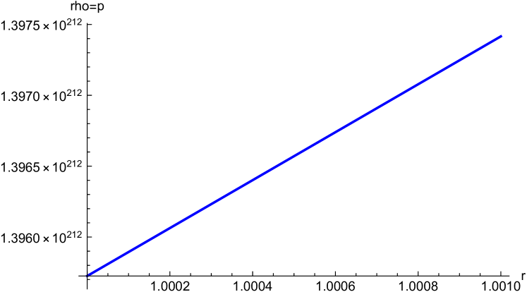
Figure 1: graphical representation of density relationship with r

3.3 Exterior Spacetime

The outer sector is described with the help of widely known static exterior Schwarzschild solution whose mathematical form is written as

$$ds^{2}=-\left(1-\frac{2M}{r}\right)^{-1}dr^{2}-r^{2}(d\theta^{2}-\sin^{2}\theta d\phi^{2})+\left(1-\frac{2M}{r}\right)dt^{2}.$$ (30)

where $M$ represents the mass of gravitational system.

4 Junction Condition

The interior sector (I) of gravastar is coupled with the exterior sector (III) at the shell. Gravastar must have flat matching in the middle of sectors (I) and (III) as mentioned by the Israel formalism [59, 60]. At the coupling surface, the metric is continuous nevertheless they may not have continuous derivatives. We can find out $S_{ij}$ by implementing the above stated formalism. Lanczos equation [61, 62, 63, 64] states $S^{i}_{j}$ as

$$S^{i}_{j}=\frac{1}{8\pi}\left(\delta^{i}_{j}\kappa^{k}_{k}-\kappa^{i}_{j}\right),$$ (31)

here $k_{ij}=K^{+}_{ij}-K^{-}_{ij}$ yield the discontinuity in the extrinsic curvatures. The inner and outer sectors are correlated by “+” and “-” signs, respectively. The second fundamental forms [65, 66, 67, 68] linked with the two borders of the shell are given by

$$K^{\pm}_{ij}=-n^{\pm}_{\nu}\left[\Gamma^{\nu}_{\alpha\beta}\frac{\partial x^{\alpha}}{\partial\xi^{i}}\frac{\partial x^{\beta}}{\partial\xi^{j}}+\frac{\partial^{2}x_{v}}{\partial\xi^{i}\partial\xi^{j}}\right]_{\Sigma},$$ (32)

where $\xi^{i}$ and $n^{\pm}_{\nu}$ represent the intrinsic coordinates of the shell and unit normal over $\Sigma$, respectively. The line element for spherical geometry is

$$ds^{2}=-\frac{dr^{2}}{f(r)}+f\left(r\right)d^{2}-r^{2}(d\theta^{2}-\sin^{2}\theta)d\phi^{2},$$ (33)

for which the unit normal $n^{\pm}_{\nu}$ can be written as

$$n^{\pm}_{\nu}=\pm\mid g^{\alpha\beta}\frac{\partial f}{\partial x^{\alpha}}\frac{\partial f}{\partial x^{\beta}}\mid^{\frac{-1}{2}}\frac{\partial f}{\partial x^{\nu}},$$ (34)

with $n^{\mu}n_{\mu}$=1. With the help of Lanczos equation, one can write $S_{ij}=diag[\sigma,-\mathbf{\nu}]$, where $\nu$ is written for the surface pressure and $\sigma$ represents surface energy density. The density distribution as well as pressure at the surface are written as

$$\sigma = -\frac{1}{4\pi D}\left[\sqrt{f}\right]^{+}_{-},$$ (35)

$$\nu = -\frac{\sigma}{2}+\frac{1}{16\pi}\left[\frac{f^{{}^{\prime}}}{\sqrt{f}}\right]^{+}_{-}.$$ (36)

By making use of the above two equations when $e^{-\lambda}=L$ and $e^{-\lambda}=A$, respectively, we get

$$\sigma = \frac{-1}{4\pi D}\left[\sqrt{1-\frac{2M}{D}}-\sqrt{L}\right],$$ (37)

$$\sigma = \frac{-1}{4\pi D}\left[\sqrt{1-\frac{2M}{D}}-\sqrt{A}\right],$$ (38)

$$\upsilon = \frac{1}{8\pi D}\left[\frac{1-\frac{M}{D}}{\sqrt{1-\frac{2M}{D}}}-\frac{2f_{R}D(L)-M}{2f_{R}D\sqrt{L}}\right],$$ (39)

$$\upsilon = \frac{1}{8\pi D}\left[\frac{1-\frac{M}{D}}{\sqrt{1-\frac{2M}{D}}}-\frac{A+B-C+E}{\sqrt{A}}\right].$$ (40)

By using Eq.(37), the thin shell mass is obtained as

$$m_{s} = D\left[\sqrt{1-\frac{1}{f_{R}}\left[\frac{k\rho_{0}D^{2}}{3}+D\int T^{0(D)}_{0}dD-\frac{2}{D}\int(\int T^{0(D)}_{0}dD)DdD\right]}\right.$$ (41)

$$- \left.\sqrt{1-\frac{2M}{D}}\right].$$

In a similar ways, from Eq.(38), the thin shell mass is obtained as

$$m_{s}=D\left[\sqrt{1-\frac{k\rho_{0}D^{2}}{3f_{R}}+\frac{k\rho_{0}}{3D}\int D^{3}(\frac{1}{f_{R}})^{{}^{\prime}}dD-\frac{1}{D}\int\frac{D^{2}}{f_{R}}T^{0(D)}_{0}dD}-\sqrt{1-\frac{2M}{D}}\right].$$ (42)

By using Eq.(39), the total mass $M$ of gravastar is found to be

$$M=\frac{D}{2}-\frac{m_{s}^{2}}{2D}-\frac{D}{2}\left[L\right]+m_{s}\sqrt{L},$$ (43)

while from Eq.(40), the total mass $M$ of gravastar is written as

$$M=\frac{-m^{2}_{s}}{2D}+\frac{D}{2}\left[1-A\right]+m_{s}\sqrt{A}.$$ (44)

5 Realistic Characteristics

This section is aimed to examine the impact of $f(R,G)$ gravity on various physical characteristics of gravastar model. In particular, we will analyze the shell’s length as well as energy of the stellar model. The entropy as well as EoS will also be discussed during the dynamical formulation of gravastars. These results would also be indicated via plots.

5.1 Proper length of the shell

We assume that shell is placed at $r=D$ which defines the phase edge of sector (I). The shell is of very small width, i.e., $\epsilon<<1$. Therefore, the sector (III) initiates from attachment at $r=D+\epsilon$. Thus, the actual width in between of these attachments of the shell is calculated by using Eq.(26) as

$$\ell=\int^{D+\epsilon}_{D}\frac{dr}{\sqrt{2lnr+c_{1}-\frac{1}{f_{R}}\left[r\int(T^{0(D)}_{0}+T^{1(D)}_{1})dr-\int(\int(T^{0(D)}_{0}+T^{1(D)}_{1})dr)dr\right]}}.$$ (45)

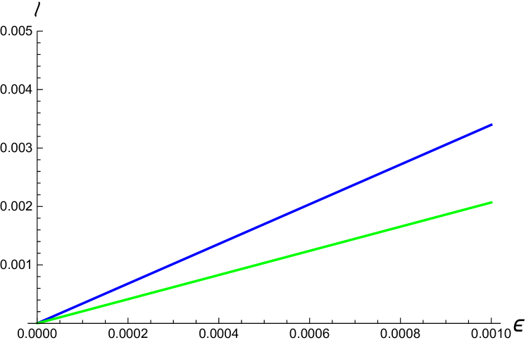
Figure 2: graphical representation of relationship between proper length $\ell$ and the thickness of shell $\epsilon$

By making use of Eq.(27), one can have

$$\ell=\int^{D+\epsilon}_{D}\frac{dr}{\sqrt{2lnr+c_{2}-\int\left(\frac{r}{f_{R}}T^{0(D)}_{0}\right)dr-\int\frac{r}{f_{R}}T^{1(D)}_{1}dr}}.$$ (46)

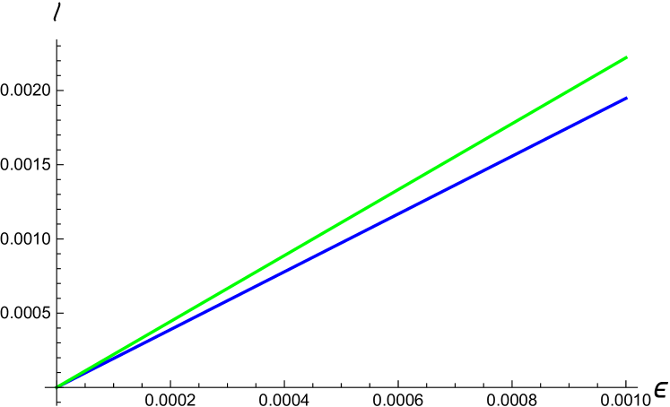
Figure 3: graphical representation of relationship between proper length $\ell$ and the thickness of shell $\epsilon$

5.1.1 Energy content

We suppose the EoS $(p=-\rho)$ for the inner sector that illustrates the zone having negative energy and approve the nature of repulsion of interior sector. But the energy inside the shell will be

$$\varepsilon=\int^{D+\epsilon}_{D}4\pi\rho r^{2}dr=4\pi H\int^{D+\epsilon}_{D}e^{-B+\int T(D^{\star})dr}r^{2}dr.$$ (47)

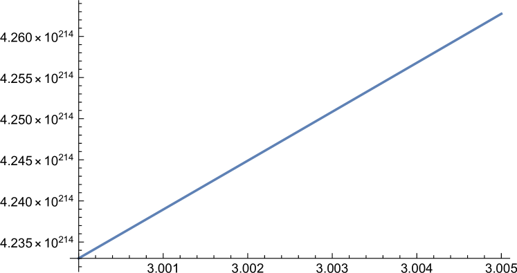
Figure 4: graphical representation of energy $\varepsilon$ relationship with thickness of shell $\epsilon$

5.1.2 Entropy

Mazur and Mottola [1] suggested that the interior sector must has zero entropy that is persistent with a specific condensate condition. Inside the shell, the entropy will be

$$S=\int^{D+\epsilon}_{D}4\pi r^{2}s(r)\sqrt{e^{\lambda}}dr.$$ (48)

The entropy of local temperature $T(r)$ is given by

$$S(r)=\frac{\alpha^{2}k^{2}_{B}T(r)}{4\pi h^{2}}=\alpha\left(\frac{k_{B}}{h}\right)\sqrt{\frac{p}{2\pi}},$$ (49)

where $\alpha$ is a constant having no dimension and $G=c=1$ with Planckian units $k_{B}=h=1$. The entropy density inside the shell will be

$$S(r)=\alpha\sqrt{\frac{p}{2\pi}}.$$ (50)

So, by using Eq.(26) in (48), we get

$$S=\sqrt{8\pi H}\alpha\int^{D+\epsilon}_{D}r^{2}\sqrt{e^{-B+\int T(D^{\star})dr}}\frac{dr}{\sqrt{Z}}.$$ (51)

In a similar manner, the use of Eq.(27) in (48) leads to

$$S=\sqrt{8\pi H}\alpha\int^{D+\epsilon}_{D}r^{2}\sqrt{e^{-B+\int T(D^{\star})dr}}\frac{dr}{\sqrt{T}}.$$ (52)

5.1.3 Equation of State

In general, the EoS at $r=D$ is given as

$$\upsilon=\omega(D)\sigma$$ (53)

By making use of Eqs.(37) and (39), we found

$$\omega(D)=\frac{\left[\frac{1-\frac{M}{D}}{\sqrt{1-\frac{2M}{D}}}-\frac{2f_{R}DL-M}{2f_{R}D\sqrt{L}}\right]}{2\left[-\sqrt{1-\frac{2M}{D}}+\sqrt{L}\right]},$$ (54)

here, $\omega(D)$ can only be real if $\frac{2M}{D}<1$ along with

$$\frac{1}{f_{R}}\left[\frac{k\rho_{0}D^{2}}{3}+D\int T^{0(D)}_{0}dD-\frac{2}{D}\int(\int T^{0(D)}_{0}dD)DdD\right]<1.$$

Also, by taking $\frac{M}{D}<<1$ and $\frac{1}{f_{R}}\left[\frac{k\rho_{0}D^{2}}{3}+D\int T^{0(D)}_{0}dD-\frac{2}{D}\int(\int T^{0(D)}_{0}dD)DdD\right]<<1$ in a binomial series and having the terms up to first order for the terms in the square-root, we obtain

$$\omega(D)\approx\frac{1-L+\frac{D}{2f_{R}}\int T^{0(D)}_{0}dD-\frac{1}{f_{R}D}\int\int(T^{0(D)}_{0}dD)DdD}{2\left[\frac{M}{D}-\frac{1}{2}(1-L)\right]}.$$ (55)

By making use of Eqs.(38) and (40), one can write

$$\omega(D)=\frac{\frac{1-\frac{M}{D}}{\sqrt{1-\frac{2M}{D}}}-\frac{A+B-C-D}{\sqrt{A}}}{2\left[\sqrt{1-\frac{2M}{D}+\sqrt{A}}\right]}.$$ (56)

Here, $\omega(D)$ can only be real if  $\frac{2M}{D}<1$ along with  $\frac{K\rho_{0}D^{2}}{3f_{R}}+\frac{K\rho_{0}}{3D}\int D^{3}(\frac{1}{f_{R}})^{{}^{\prime}}dD+\frac{1}{D}\int\frac{D^{2}}{f_{R}}T^{0(D)}_{0}dD<1$. Also, if one elaborate the square-root terms of Eq.(57) by taking $\frac{M}{D}<<1$ and $\frac{K\rho_{0}D^{2}}{3f_{R}}+\frac{K\rho_{0}}{3D}\int D^{3}(\frac{1}{f_{R}})^{{}^{\prime}}dD+\frac{1}{D}\int\frac{D^{2}}{f_{R}}T^{0(D)}_{0}dD<<1$ in a binomial series and having the terms up to first order, then we get

$$\omega(D)\approx{\frac{\frac{2K\rho_{0}D^{2}}{3f_{R}}+\frac{D^{2}}{2f_{R}}T^{0(D)}_{0}+....}{2\left[\frac{M}{D}-\frac{K\rho_{0}D^{2}}{6f_{R}}+....\right]}}.$$ (57)

6 Conclusion

In this paper, we have demonstrated a particular stellar model which was initially theorized by Mazur and Mottola [1] under the influence of $f(R,G)$ gravity. The stellar model named as gravastar can be studied as a feasible alternate to the black hole structure. The gravastar can be characterized by three distinct sectors; inner sector, intermediate thin shell and outer sector with particular EoS for every sector. With the help of this description, we have calculated a definite solution which is free of singularity for the gravastar and demonstrated it with different physically feasible properties within the scheme of $f(R,G)$ gravity.

We have written down distinct important features of the solution set as follows:

1. Density-pressure relationship: The relation of pressure of the ultra-relativistic matter present in the shell with its density is shown corresponding to its radius in Fig.1 which sustains a consistent diversity in every part of the shell.

2. Proper length: Relationship between proper length $\ell$ and thickness of shell ($\epsilon$)(in Fig.2) shows the continuous increase (constant case).

3. Proper length: Relationship between proper length $\ell$ and thickness of shell ($\epsilon$) (in Fig.3) shows the continuous increase (variable case). More precisely, the influence of $f(R,G)$ is responsible to increase the length of the shell.

4. Energy content: Figure 4 shows that the energy of the shell has direct relation corresponding to the thickness of the shell $\epsilon$.

Declaration of Competing Interest

The authors declare that they have no known competing financial interests or personal relationships that could have appeared to influence the work reported in this paper.

Acknowledgement

The work of MZB and ZY was supported by National Research Project for Universities (NRPU), Higher Education Commission, Pakistan under research project No. 8769/Punjab/ NRPU/R$\&$D/HEC/2017. The authors would like to thank the anonymous reviewer for the valuable and constructive comments and suggestions in order to improve the quality of the paper.

7 Appendix:

$$L =1-\frac{1}{f_{R}}\left[\frac{k\rho_{0}D^{2}}{3}+D\int T^{0(D)}_{0}dD-\frac{2}{D}\int(\int T^{0(D)}_{0}dD)DdD\right],$$

$$M =2K\rho_{0}D^{3}+D^{2}\int T^{0(D)}_{0}dD+D^{3}T^{0(D)}_{0}-2D^{2}\int T^{0(D)}_{0}dD$$

$$+2\int(\int T^{0(D)}_{0}dD)DdD,$$

$$A =1-\frac{K\rho_{0}D^{2}}{3f_{R}}+\frac{K\rho_{0}}{3D}\int D^{3}\left(\frac{1}{f_{R}}\right)^{{}^{\prime}}dD+\frac{1}{D}\int\frac{D^{2}}{f_{R}}T^{0(D)}_{0}dD,$$

$$B =\frac{K\rho_{0}D}{6}\left[\frac{-2Df_{R}+D^{2}(f_{R})^{{}^{\prime}}}{(f_{R})^{2}}\right],$$

$$C =\frac{K\rho_{0}D}{6}\left[\frac{-1}{D^{2}}\int D^{3}\left(\frac{1}{f_{R}}\right)^{{}^{\prime}}dD+D^{2}\left(\frac{1}{f_{R}}\right)^{{}^{\prime}}\right],$$

$$T =2lnr-\int\frac{r}{f_{R}}(T^{0(D)}_{0}+T^{1(D)}_{1})dr+c_{6},$$

$$E =\frac{D}{2}\left[\frac{-1}{D^{2}}\int\frac{D^{2}}{f_{R}}T^{0(D)}_{0}dD+\frac{D}{f_{R}}T^{0(D)}_{0}\right],$$

$$Z ={2lnr-\frac{1}{f_{R}}[r\int(T^{0(D)}_{0}+T^{1(D)}_{1})dr-\int(\int(T^{0(D)}_{0}+T^{1(D)}_{1}dr)dr)]+c_{5}},$$

$$T^{(D^{\star})} =\frac{1}{PKe^{-\lambda}}\left[-T^{11(D)^{\prime}}-\frac{e^{\nu}\nu^{\prime}}{2e^{\lambda}}T^{00(D)}-\lambda^{\prime}T^{11(D)}+\frac{r}{e^{\lambda}}T^{22(D)}-\frac{\nu^{\prime}}{2}T^{11(D)}\right.$$

$$-\left.\frac{2}{r}T^{11(D)}+\frac{r}{e^{\lambda}}T^{22(D)}\right].$$

References

- [1] P. O. Mazur and E. Mottola Proc. Natl. Acad. Sci. U.S.A, vol. 101, p. 9545, 2004.
- [2] F. S. N. Lobo and R. Garattini J. High Energy Phys., vol. 2013, no. 12, p. 65, 2013.
- [3] K. K. Nandi, Y. Z. Zhang, R. G. Cai, and A. Panchenko Phys. Rev. D, vol. 79, no. 2, p. 024011, 2009.
- [4] D. Horvat and S. Ilijić Class. Quantum Grav., vol. 24, no. 22, p. 5637, 2007.
- [5] A. DeBenedictis, D. Horvat, S. Ilijić, S. Kloster, and K. Viswanathan Class. and Quantum Grav., vol. 23, no. 7, p. 2303, 2006.
- [6] N. Bilić, G. B. Tupper, and R. D. Viollier J. Cosmol. Astropart. Phys, vol. 2006, no. 02, p. 013, 2006.
- [7] M. Visser and D. L. Wiltshire Class. Quantum Gravity, vol. 21, no. 4, p. 1135, 2004.
- [8] F. S. N. Lobo and A. V. B. Arellano Class. Quantum Grav., vol. 24, no. 5, p. 1069, 2007.
- [9] P. Rocha, R. Chan, M. F. A. da Silva, and A. Wang J.Cosmol. Astropart. Phys., vol. 2008, no. 11, p. 010, 2008.
- [10] M. Z. Bhatti, Z. Yousaf, and M. Ajmal Int. J. Mod. Phys. D, vol. 28, p. 1950123, 2019.
- [11] M. Z. Bhatti Mod. Phys. Lett. A, vol. 35, p. 2050069, 2020.
- [12] Z. Yousaf, K. Bamba, M. Z. Bhatti, and U. Ghafoor Phys. Rev. D, vol. 100, p. 024062, 2019.
- [13] Z. Yousaf, M. Z. Bhatti, and H. Asad Phys. Dark Universe, vol. 28, p. 100527, 2020.
- [14] Z. Yousaf Phys. Dark Universe, vol. 28, p. 100509, 2020.
- [15] A. G. Riess, A. V. Filippenko, P. Challis, A. Clocchiatti, A. Diercks, P. M. Garnavich, R. L. Gilliland, C. J. Hogan, S. Jha, R. P. Kirshner, et al. Astron. J., vol. 116, no. 3, p. 1009, 1998.
- [16] S. Perlmutter, G. Aldering, G. Goldhaber, R. A. Knop, P. Nugent, P. Castro, S. Deustua, S. Fabbro, A. Goobar, D. Groom, et al. The Astrophys. J., vol. 517, no. 2, p. 565, 1999.
- [17] P. de Bernardis, P. A. R. Ade, J. J. Bock, J. Bond, J. Borrill, A. Boscaleri, K. Coble, B. Crill, G. De Gasperis, P. C. Farese, et al. Nature, vol. 404, no. 6781, p. 955, 2000.
- [18] P. J. E. Peebles and B. Ratra REv. Mod. Phys, vol. 75, no. 2, p. 559, 2003.
- [19] H. A. Buchdahl Mon. Not. R. Astron. Soc, vol. 150, no. 1, p. 1, 1970.
- [20] S. Nojiri and S. D. Odintsov Phys. Rep, vol. 505, no. 2-4, p. 59, 2011.
- [21] M. Baibosunov, V. T. Gurovich, and U. Imanaliev JETP, vol. 71, no. 4, p. 636, 1990.
- [22] T. Harko MoN. NoT. R. Astron. Soc, vol. 413, no. 4, p. 3095, 2011.
- [23] D. Lovelock J. Math. Phys, vol. 12, no. 3, p. 498, 1971.
- [24] K. Bamba, M. Ilyas, M. Bhatti, and Z. Yousaf Gen. Relativ. Gravit., vol. 49, no. 8, p. 112, 2017.
- [25] M. F. Shamir and M. Ahmad Eur.Phys.J.C, vol. 77, no. 1, p. 1, 2017.
- [26] M. F. Shamir and M. Ahmad Mod.Phys.Lett.A, vol. 32, no. 16, p. 1750086, 2017.
- [27] B. Li, J. D. Barrow, and D. F. Mota Phys.Rev.D, vol. 76, no. 4, p. 044027, 2007.
- [28] J. M. Lattimer and A. W. Steiner Astrophys.J, vol. 784, no. 2, p. 123, 2014.
- [29] T. Jaffe, A. Banday, J. Leahy, S. Leach, and A. Strong MoN.NoT.R.Astron.Soc, vol. 416, no. 2, p. 1152, 2011.
- [30] A. De Felice and S. Tsujikawa Phys. Lett., vol. 675, no. 1, p. 1, 2009.
- [31] M. Alimohammadi and A. Ghalee Phys.Rev.D, vol. 79, no. 6, p. 063006, 2009.
- [32] C. G. Boehmer and F. S. Lobo Phys.Rev.D, vol. 79, no. 6, p. 067504, 2009.
- [33] K. Uddin, J. E. Lidsey, and R. Tavakol Gen.Relativ.Gravit, vol. 41, no. 12, p. 2725, 2009.
- [34] M. Z. Bhatti and Z. Tariq Phys. Dark Universe, vol. 28, p. 100482, 2020.
- [35] Z. Yousaf, M. Z. Bhatti, and T. Naseer Phys. Dark Universe, vol. 28, p. 100535, 2020.
- [36] M. Z. Bhatti, Z. Yousaf, and M. Yousaf Phys. Dark Universe, vol. 28, p. 100501, 2020.
- [37] A. De Felice and T. Tanaka Prog. Theor. Phys., vol. 124, p. 503, 2010.
- [38] A. De Felice, T. Suyama, and T. Tanaka Phys. Rev., vol. 83, no. 10, p. 104035, 2011.
- [39] A. De la Cruz-Dombriz and D. Sáez-Gómez Class. Quantum Gravity, vol. 29, no. 24, p. 245014, 2012.
- [40] M. De Laurentis and A. J. Lopez-Revelles Int. J. Geom. Methods. Mod. Phys., vol. 11, no. 10, p. 1450082, 2014.
- [41] M. Houndjo, M. Rodrigues, D. Momeni, and R. Myrzakulov Can. J. Phys., vol. 92, no. 12, p. 1528, 2014.
- [42] K. Atazadeh and F. Darabi Gen. Relativ. Gravit., vol. 46, no. 2, p. 1664, 2014.
- [43] M. De Laurentis, M. Paolella, and S. Capozziello Phys. Rev., vol. 91, p. 083531, 2015.
- [44] S. D. Odintsov, V. K. Oikonomou, and S. Banerjee Nucl. Phys., vol. 938, p. 935, 2019.
- [45] S. H. Shekh, S. Arora, V. R. Chirde, and P. K. Sahoo Int. J. Geom. Meth. Mod. Phys., vol. 17, p. 2050048, 2020.
- [46] R. Myrzakulov, D. Sáez-Gómez, and A. Tureanu Gen. Relativ. Gravit., vol. 43, no. 6, p. 1671, 2011.
- [47] M. Z. Bhatti, Z. Yousaf, and M. Ilyas Eur. Phys. J. C, vol. 77, p. 690, 2017.
- [48] Z. Yousaf, M. Sharif, M. Ilyas, and M. Z. Bhatti Eur. Phys. J. C, vol. 77, no. 10, p. 691, 2017.
- [49] Z. Yousaf, K. Bamba, and M. Z. Bhatti Phys. Rev. D, vol. 95, p. 024024, 2017.
- [50] Z. Yousaf, M. Z. Bhatti, and S. Yaseen Eur. Phys. J. Plus, vol. 134, p. 487, 2019.
- [51] Z. Yousaf, M. Z. Bhatti, and M. F. Malik Eur. Phys. J. Plus, vol. 134, p. 470, 2019.
- [52] E. Elizalde, S. D. Odintsov, V. K. Oikonomou, and T. Paul Nucl. Phys. B, vol. 954, p. 114984, 2020.
- [53] D. Psaltis Living. Rev. Relativ., vol. 11, no. 1, p. 9, 2008.
- [54] M. S. Madsen, J. P. Mimoso, J. A. Butcher, and G. F. Ellis Phys. Rev. D, vol. 46, no. 4, p. 1399, 1992.
- [55] P. S. Wesson J. Math. Phys., vol. 19, no. 11, p. 2283, 1978.
- [56] T. M. Braje and R. W. Romani Astrophys. J, vol. 580, no. 2, p. 1043, 2002.
- [57] L. P. Linares, M. Malheiro, and S. Ray Int. J. Mod. Phys. D, vol. 13, no. 07, pp. 1355–1359, 2004.
- [58] W. Israel Nuovo Cimento, vol. 48, p. 463, 1967.
- [59] G. Darmois Gauthier-Villars, Paris, vol. 25, 1927.
- [60] W. Israel I, vol. 44, no. 1, pp. 1–14, 1966.
- [61] K. Lanczos Ann.Phys.(Berl.), vol. 379, no. 14, pp. 518–540, 1924.
- [62] N. Sen Ann.Phys.(Berl.), vol. 378, no. 5-6, pp. 365–396, 1924.
- [63] G. Perry and R. B. Mann Gen. Relativ. Gravit., vol. 24, no. 3, p. 305, 1992.
- [64] P. Musgrave and K. Lake Classical Quantum Gravity, vol. 13, no. 7, p. 1885, 1996.
- [65] F. Rahaman, M. Kalam, and S. Chakraborty Gen. Relativ. Gravit., vol. 38, no. 11, p. 1687, 2006.
- [66] A. A. Usmani, Z. Hasan, F. Rahaman, S. A. Rakib, S. Ray, and P. K. F. Kuhfittig Gen. Relativ. Gravit., vol. 42, no. 12, p. 2901, 2010.
- [67] G. A. S. Dias and J. P. S. Lemos Phys. Rev. D, vol. 82, no. 8, p. 084023, 2010.
- [68] F. Rahaman, P. Kuhfittig, M. Kalam, A. A. Usmani, and S. Ray Class. Quantum Grav., vol. 28, no. 15, p. 155021, 2011.