A Revised Generative Evaluation of Visual Dialogue

Abstract

Evaluating visual dialogue (vd), the task of answering a sequence of questions relating to a visual input, remains an open research challenge. The current evaluation scheme of the VisDial dataset computes the ranks of ground-truth answers in predefined candidate sets, which Massiceti et al. (2018) show can be susceptible to the exploitation of dataset biases. This scheme also does little to account for the different ways of expressing the same answer—an aspect of language that has been well studied in nlp. We propose a revised evaluation scheme for the VisDial dataset leveraging metrics from the nlp literature to measure consensus between answers generated by the model and a set of relevant answers. We construct these relevant answer sets using a simple and effective semi-supervised method based on correlation, which allows us to automatically extend and scale sparse relevance annotations from humans to the entire dataset. We release these sets and code for the revised evaluation scheme as DenseVisDial and intend them to be an improvement to the dataset in the face of its existing constraints and design choices.

1 Introduction

Question Answer How old is the baby? About 2 years old What color is the remote? White Where is the train? On the road How many cows are there? Three

Figure 1: Failures in visual dialogue (from Massiceti et al. (2018))—answers are unrelated to the image. Biases in the VisDial dataset, compounded by a rank-based evaluation, can mislead progress on the vd task.

The growing interest in visual conversational agents (Antol et al., 2015; Das et al., 2017; De Vries et al., 2017; Johnson et al., 2017) has motivated the need for automated evaluation metrics for the responses generated by these agents. Robust evaluation schemes, however, are an open research challenge (Mellish and Dale, 1998; Reiter and Belz, 2009). This is the case for VisDial (Das et al., 2017), a dataset targeting the visual dialogue (vd) task—answering a sequence of questions about an image given a history of previous questions and answers. At test time, a trained model is used to score fixed sets of candidate answers for each test question, and a suite of rank-based metrics are computed on the ranked sets: single-candidate metrics which are a function of the ground-truth (gt) answer’s position, and a multi-candidate metric which weighs the ranked set with relevance scores assigned from human annotation. A limit of this scheme is that a simple model (Massiceti et al., 2018) based on canonical correlation analysis (cca), which learns to maximise correlation between questions and answers while completely ignoring the image and dialogue history, is comparable in mean rank (mr)—one of the dataset’s primary rank-based metrics—to state-of-the-art (sota) models, all of which employ complex neural network architectures of millions of parameters, requiring many hours of gpu(s) training. This suggests that exploitable biases exist within the VisDial dataset, whose effects are compounded by a rank-based evaluation ill-suited to the vd task.

Motivated by this, we propose a revised, more robust, evaluation scheme for the vd task, informed by the key shortfalls of the current evaluation, namely that 1) the candidate sets contain multiple, equally feasible answers, rendering both single- and multi-candidate ranking metrics less meaningful, and 2) the evaluation is an indirect ranking task, rather than a direct assessment of the answers generated by a model—the goal of a vd agent.

Our revised evaluation instead adopts standard metrics from nlp to measure the similarity between an answer generated by a model and a reference set of answers for the image and question. This aligns better with the generative nature of a true vd agent, and with established evaluation set-ups for other language generations tasks, including vqa (Antol et al., 2015) and image captioning (Chen et al., 2015; Young et al., 2014). Unlike the current evaluation, it also accounts for diversity in answer generations, which we compare across models.

For VisDial, however, the answer relevance scores used to construct the reference sets are only available for a small subset of the dataset. Drawing on the pseudo-labelling literature for semi-supervised learning (Lee, 2013; Wu and Yap, 2006; Iscen et al., 2019), we develop a semi-supervised approach which leverages these human annotations, and automatically learns to extract the relevant answers from a given candidate set. We apply cca between pre-trained question and answer features, channelling Massiceti et al. (2018), and use a clustering heuristic on the resulting correlations to extract the candidate answers most correlated with the ground-truth answer—the reference sets, or pseudo-labels. This was inspired by prior work showing the surprising strength of simple, non-deep baselines (Zhou et al., 2015; Massiceti et al., 2018; Strang et al., 2018; Anand et al., 2018). Using this approach, we automatically construct sets of relevant answers for the entire VisDial dataset, which we validate in multiple ways, including with human judgements via Amazon Mechanical Turk (amt), and release as DenseVisDial—a dense version of VisDial. Using this data and the revised scheme, we re-evaluate existing sota models and gain new insights into model differences, specifically generation diversity, otherwise unavailable with the existing evaluation. The scheme also improves on the existing multi-candidate ranking evaluation, only applicable for $1/10$ of the dataset due to the cost and time of collecting relevance scores from humans. Finally, while we use these reference sets exclusively for better evaluation purposes, we also show that using them as (for-free) additional training data can improve performance, which is promising for future progress on the vd task.

To summarise, our contributions are:

1. A revised evaluation scheme for the VisDial dataset based on metrics from nlp which measure the similarity between a generated answer and a reference set of feasible answers.

2. A semi-supervised method for automatically extracting these reference sets from given candidate sets at scale, verified using human annotators.

3. An expanded DenseVisDial data with the automatically constructed reference sets, released for future evaluation and model development.

2 Preliminaries

We first define generative vd (for VisDial), and how Massiceti et al. (2018) employ cca for this.

2.1 Visual Dialogue (vd) & VisDial dataset

Given image $I$ and dialogue history $[(Q_{1},A_{1}),(Q_{2},A_{2}),\ldots,Q_{i}]$, the generative vd task involves generating answer $A_{i}$.

The principal approach towards vd has been facilitated by the VisDial dataset (Das et al., 2017), a large corpus of images paired with question-answer dialogues, sequentially collected by pairs of annotators in an interactive game on amt. VisDial v1.0 comprises $123,287/2064/8000$ train/val/test images, each paired with dialogues of up to 10 exchanges. Each question is coupled with a candidate set of 100 answers $\bm{A}$ including a ground-truth answer $A_{\text{gt}}\in\bm{A}$. For a subset (2000/2064/8000), one question per image contains human-annotated relevance scores $\rho(A)\in[0,1]\,\text{where\,}A\in\bm{A}$.

The generative vd task learns to generate answers conditioned on image-question pairs using only $(I,Q,A_{\text{gt}})$ triplets (Das et al., 2017). At test time, given an image-question pair, each answer in its associated candidate answers $\bm{A}$ is scored under the model’s learned likelihood. The rank of $A_{\text{gt}}$ is then used to judge the model’s effectiveness at the vd task, averaged over the dataset to get the mr. Other metrics also computed include normalised discounted cumulative gain (ndcg) on the candidate answers’ human-annotated relevance scores.

In a second paradigm introduced by Das et al. (2017), the model instead uses the full $(I,Q,\bm{A})$ at train time, and simply frames the predictive task as a classification problem of selecting $A_{\text{gt}}$ out of $\bm{A}$. At test time, the candidates are then directly scored by the classifier’s softmax probabilities. We argue that this discriminative setting is an over-simplification of the vd task: answering questions is not simply selecting the correct answer from a set. The focus of the remainder of this paper is therefore fully on the generative vd task.

2.2 Canonical Correlation Analysis for vd

cca, applied between question and answers, achieves near-sota mean rank (mr) on the VisDial dataset (Massiceti et al., 2018). Inspired by this result and the extreme simplicity of cca, we introduce this formulation with reference to vd.

Given paired observations $\{\mathbf{x}_{1}\in\mathbb{R}^{n_{1}},\mathbf{x}_{2}\in\mathbb{R}^{n_{2}}\}$, cca jointly learns projections $W_{1}\in\mathbb{R}^{n_{1}\times k}$ and $W_{2}\in\mathbb{R}^{n_{2}\times k}$, $k\leq\min(n_{1},n_{2})$, which are maximally correlated (Hotelling, 1936). Projections are obtained via a generalised eigenvalue decomposition, $A\bm{v}=\lambda B\bm{v}$ (Kettenring, 1971; Hardoon et al., 2004; Bach and Jordan, 2002), where $A$ and $B$ are the inter- and intra-view correlation matrices. Projection matrix $W_{i}\in^{n_{i}\times k}$ embeds $\mathbf{x}_{i}$ from view $i$ as $\phi(\mathbf{x}_{i};W_{i})=D_{\bm{\lambda}}^{p}W_{i}^{\top}\mathbf{x}_{i}$, where $D_{\lambda}$ is a diagonal matrix of the top $k$ (sorted) eigenvalues $\bm{\lambda}$, and $p$ is a scalar weight. With cca, ranking and retrieval across views $\{\mathbf{x}_{i},\mathbf{x}_{j}\}$ is performed by computing correlation between projections $\mathrm{corr}(\mathbf{x}_{i},\mathbf{x}_{j})=\frac{\psi(\mathbf{x}_{i})^{\top}\psi(\mathbf{x}_{j})}{\left\lVert\psi(\mathbf{x}_{i})\right\rVert_{2}\left\lVert\psi(\mathbf{x}_{j})\right\rVert_{2}}$ where $\psi$ is a mean-centred (over train set) version of $\phi$.

Using cca, learnt embeddings between answers and questions (cca -aq) are used to compute the ranking and ndcg metrics. cca can also be used to generate answers using correlations. For a given test question, its $100$ nearest-neighbour questions (based on correlation under the A-Q model) are extracted from the train set. Their $100$ corresponding ground-truth answers are used to construct a pseudo-candidate set. Answers are generated by the model, denoted cca -aq-g, by sampling from this set in proportion to correlation with the test question (see Figure 3 in Massiceti et al. (2018)).

3 ​​Shortfalls of Current VisDial Evaluation​​

The fact that a simple, lightweight cca model performs favourably in mr with current sota models, while completely ignoring the image and dialogue history, and requiring an order of magnitude fewer learnable parameters and mere seconds on cpu to train, is a cause for concern. Not only do prior results suggest that implicit correlations between just the questions and answers exist in the data (see Figure 1), but also that the current evaluation scheme generally is not flexible enough to account for variation in answers to visually-grounded questions. Here we summarise the existing evaluation scheme, discuss the hidden factors affecting it, and make the case that to better capture a model’s performance on the vd task, there must be changes to the evaluation scheme.

3.1 Current evaluation scheme

Given a test question, the current VisDial evaluation relies on ranking its candidate answers (Das et al., 2017), derived from scoring the answers under the trained (generative) model’s likelihood (see § 2.1).

A suite of rank-based metrics is then computed: mean rank (mr)and mean reciprocal rank (mrr) of the ground truth (gt) answer over data, and the average recall, measuring how often the gt answer falls within the top 1, 5, and 10 ranks, respectively. These single-candidate (i.e. gt) ranking metrics have been the norm since VisDial’s inception.

A subsequent extension of the dataset (v1.0) tasked 4-5 human annotators with labelling whether each answer in a candidate set is valid for a given image-question (a hard 0/1 choice) for a subset of the train and validation sets, denoted $\mathcal{H}_{t}$ and $\mathcal{H}_{v}$, respectively. For each candidate answer $A$, the mean judgement across annotators becomes a relevance score $\rho(A)\in[0,1]$. A modified multi-candidate ranking metric, the ndcg, is then introduced: candidate answers’ ranks are weighted by their relevance scores, excluding irrelevant ($\rho(A)=0$) answers. See Appendix B for further details.

3.2 Analysing current shortfalls

The above evaluation metrics, by construction, are not flexible enough to account for the many ways a question can satisfactorily be answered. This limitation manifests in both the single- and multi-candidate ranking metrics, and hampers the measurement of a model’s true ability to answer a visual question. The limitation stems from:

1. ranking candidate sets that are ill-constructed for the ranking task, and

2. disregarding answers generated by a model in favour of indirectly ranking these fixed sets.

3.2.1 Ranking ill-constructed candidate sets

Candidate answer sets in VisDial are typically observed to contain multiple feasible answers—as they include up to 50 nearest-neighbour answers (Das et al., 2017) to $A_{\text{gt}}$ in GloVe (Pennington et al., 2014) space. Rank-based metrics, which assume a meaningful ordering of answers, are less informative when considering feasible-answer subsets.

We explicitly verify this characteristic of candidate answers using correlation, through the following experiment which learns a cca model between the question and answer features. Computing the correlation between $A_{\text{gt}}$ and $A\in\bm{A}\setminus A_{\text{gt}}$, giving $\mathcal{C}=(\phi(A_{\text{gt}},A_{1}),\ldots,\phi(A_{\text{gt}},A_{100}))$, we then select the cluster of answers with correlations in $[\mathcal{C}_{\text{max}}-\sigma,\mathcal{C}_{\text{max}}],\text{where\,\,}\mathcal{C}_{\text{max}}\!=\!\mathrm{max}(\mathcal{C}),\sigma\!=\!\mathrm{stdev}(\mathcal{C})$, roughly estimating answers which are plausibly similar to $A_{\text{gt}}$. Given this cluster, we compute the mean and standard deviation of the correlations, as well as the cluster size, to measure how small and tightly packed these clusters are. We average these across all candidate sets, giving an average mean correlation of $0.58$, an average standard deviation of $0.22$, and an average cluster size of $12.30$. These results support the idea that an equivalence class of feasible answers exist within each candidate set, which can then adversely affect both classes of metrics described below.

Single-candidate ranking metrics assign a single answer, the labelled gt, as the only correct answer in the candidate set, and are purely a function of this privileged answer’s rank. As a result, these metrics unduly penalise models that rank alternate, but equally feasible, answers highly. Mr, mrr, and r@1,5,10 are thus only weakly indicative of performance on the vd task, and are unable to differentiate between equally good models.

The ill-constructed candidate sets also render single-candidate metrics unable to rule out poor models. In other words, models with poor mr, mrr and r@1,5,10 aren’t necessarily poor at vd. This is markedly the case for mrr and r@1,5,10 which are, by definition, biased toward low ranks—a model predicting five gt answers at rank 1, and five at rank 10, scores better mrr/r@1,5,10 than a model with all ten gt answers at rank 2 (coincidentally, these results are meaningless if the candidate set contained $10$ equally feasible answers). This bias particularly affects models trained with a single-answer objective (i.e. all sota) models. To see why, we show the distribution of gt answer ranks between cca -aq and a sota model in Figure 2. The sota model is skewed toward the gt answer achieving rank 1—the combined result of a single-answer objective and high parametrisation. This leads sota models to view other feasible answers in the set as no different if ranked 2 or 100. cca -aq by contrast ignores rank and simply learns by maximising A-Q correlation, likely leading it to rank other feasible answers highly. Thus, models favouring low ranks by virtue of their learning objective may achieve better mrr/r@1,5,10, but not be discernibly better than models accounting for multiple answers being correct.

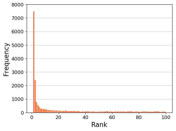
(a) hrea-qih-g

(b) cca -aq

Figure 2: Distribution of gt answer ranks across VisDial v1.0 val set. Highly-parametrised sota models (a) pushes the gt rank towards 1, ignoring other potentially feasible answers, in contrast to cca -aq (b).

These findings, together, suggest that the single-candidate metrics cannot reliably quantify performance and compare models in lieu of the vd task.

Multi-candidate ranking metrics, or ndcg, undoubtedly take a step in the right direction by forgoing just a single correct answer, and weighting the predicted ranking with human-annotated relevance scores for multiple answers. ndcg, however, is still a function of a ranking, and hence assumes that a single optimal ordering of candidate answers exists. The presence of multiple equally feasible answers in the candidate sets thus breaks this assumption and can skew the ndcg, albeit to a lesser degree than mr, mrr, and r@1,5,10.

Moreover, the degree of answer similarity within these subsets raises further concerns for the reliable computation of ndcg. Requiring annotation of 100 valid (i.e. similar) answers is an arduous task, and converting hard 0/1 judgements into relevance scores over just a handful (4-5) of annotators can be noisy. Our analysis reveals the following quirks:

• $18.15\%$/$47.14\%$ of the validation/train annotated subsets ($\mathcal{H}_{v}$/ $\mathcal{H}_{t}$), do not have a single candidate answer with relevance score $1.0$, not even the ground-truth, indicating poor consensus.

• 20.69%/9.01% of samples, respectively, consider the ground-truth irrelevant ($\rho(A_{\text{gt}})=0$).

Coupled with this, the scale of VisDial makes obtaining annotations a daunting (and expensive) task—reflected in the fact that only a small fraction of the data, one question per image, has annotations (see § 2), which implies evaluations effectively ignore dialogue history. Also, without more annotators (and hence cost/time), obtaining relevance scores at-scale may well be meaningless.

3.2.2 Ignoring generated answers

The ultimate goal of vd is to produce an answer to a given question, not to pick an answer from a set—our primary motivation for focussing on the generative vd task. The current evaluation, rather than directly evaluating the answers generated by a model, evaluates by how well a model ranks a fixed set of candidate answers. Not only is this problematic because of the candidate sets’ limitations (as described above), but also because it: 1) disregards diversity in answer generations, a necessary feature for a human-like answering agent, and 2) goes against established practice in the vqa literature (Antol et al., 2015) which evaluates by comparing the predicted answer to answers collected from 10 human annotators. While it is expected that scoring a valid answer by its likelihood is a reasonable measure of a model’s ability to generate a good answer, this may not necessarily be the case when there are multiple potential answers, some not even in the candidate set. Although likelihoods can serve as a relative measure between candidates, the highest-probability answers may be entirely different or unrelated—indicating a poorly learnt model. This supports the idea that a metric which ignores generated answers may fail to account for models no less “good” at the vd task.

4 A Revised Evaluation for VisDial

The analysis in § 3 indicates that an evaluation well matched to the underlying goals of vd should:

1. directly use answers generated by the model,

2. account for multiple valid answers, and

3. do the above at scale over the entire dataset.

We thus develop a revised evaluation scheme for vd which meets these three criteria. Its basis lies in measuring how similar an answer generated by a given model is to a set of feasible reference answers for a given question and image. We describe similarity quantification in § 4.1 and the construction of high-quality reference sets in § 4.2.

4.1 Measuring similarity

We measure similarity using established nlp consensus metrics between a predicted answer and a reference set of valid answers. Crucially, the predicted answer is generated by the model directly, and the reference set contains more than one element, accounting for the presence of multiple valid answers. We use two classes of metric for capturing consensus: overlap and embedding distance.

Overlap-based metrics compute the overlap or co-occurrence of $n$-grams (word couplets of size $n$) between pairs of sentences—here, the generated answer and each answer in the reference set. We use two such metrics: cider (Vedantam et al., 2015) and meteor (Denkowski and Lavie, 2014), motivated by their extensive use in image captioning benchmarks (Chen et al., 2015; Hodosh et al., 2013; Young et al., 2014). Both are known to be well correlated with human judgements. cider computes the cosine similarity between a pair of vectors, each of which is composed of the term-frequency inverse-document-frequencies (tf-idf) of the sentence’s $n$-grams. For $0<n\leq i$, similarities are averaged over all $n$-grams up to length $i$. meteor is similar, but first applies a uni-gram matching function, before computing a weighted harmonic mean between uni-gram precision and recall, with a fragmentation penalty on the matching.

Embedding distance-based metrics arise from a rich literature in capturing semantic similarity between natural language expressions (Bojanowski et al., 2017; Pennington et al., 2014; Devlin et al., 2019; Peters et al., 2018; Sharma et al., 2017). Motivated by the recent successes of bert (Devlin et al., 2019) and FastText (Bojanowski et al., 2017) in a variety of nlp tasks, we use each method to embed the generated answer and each reference set answer, computing the $L_{2}$ and cosine similarity (CS) between them, averaging over the reference set. The embedding metrics aim to complement the overlap-based metrics and guard against limitations of the latter that might arise due to answer lengths (one- or two-word) frequently seen in the vd data.

4.2 Obtaining answer reference sets

We now describe how to obtain reference sets for the similarity measures defined above.

4.2.1 Using humans

For a small subset of the VisDial validation set, $\mathcal{H}_{v}$, soft relevance scores are available (from human annotators) for each of the 100 candidate answers associated with each image-question (see § 2.1). Using these scores, we construct answer reference sets for each image-question, composed of all the candidate set answers deemed valid by at least one annotator, i.e. $\rho(A)>0$, where to our surprise, we found multiple instances where $\rho(A_{\text{gt}})=0$. Protecting against such cases, we define the human-annotated reference set $H=\{A:\rho(A)>0,\forall A\in\bm{A}\}\cup\{A_{\text{gt}}\}$.

4.2.2 Using semi-supervision at scale

Human-annotated relevance scores, and hence reference sets, however, are available for only a fraction of the dataset—less than 1% of questions! The scale of VisDial—on the order of $10^{6}$ questions, each with $100$ candidate answers—makes extending these annotations to the entire dataset extremely challenging. Assuming $\$0.05$ per question, each presented to $10$ workers, would incur a cost of over $\$500,000$ and substantial annotation time!

We therefore propose a semi-supervised approach which harnesses the annotations we do have: given a candidate set of answers for an image-question, we learn to extract the valid answers, and hence automatically construct a reference set. Not only does this enable us to obtain reference sets at scale, but it also circumvents the time, cost and idiosyncrasies associated with human annotation.

Our approach is based on cca, and uses the relevance-annotated subset of the full train set, $\mathcal{H}_{t}$, as training data. Similar to § 4.2.1, we construct training reference sets $H_{t}$ using $\mathcal{H}_{t}$. Pairing each question with all answers in $H_{t}$, we learn a cca model between the questions and answers. With this model, denoted cca -aq^*, we compute correlations between $A_{\text{gt}}$ and $\bm{A}\setminus A_{\text{gt}}$, giving $\mathcal{C}=(\phi(A_{\text{gt}},A_{1}),\ldots,\phi(A_{\text{gt}},A_{100}))$ similar to § 3. We then cluster these correlations in $\mathcal{C}$ to construct a reference set $\Sigma=\{A:\phi(A_{\text{gt}},A)\in[\mathcal{C}_{\text{max}}-\sigma,\mathcal{C}_{\text{max}}]\}\cup\{A_{\text{gt}}\}$ where $\mathcal{C}_{\text{max}}=\mathrm{max}(\mathcal{C})$, and $\sigma=\mathrm{stdev}(\mathcal{C})$. Intuitively, this extracts the cluster of answers with highest correlation or similarity to the ground-truth answer. With this semi-supervised approach, we easily and quickly obtain reference sets at scale for the entire VisDial dataset.

Verifying automatic reference sets

The validity of the revised evaluation is contingent on the validity of the automatic reference sets—that they are composed of valid answers. We verify this by:

1. computing intersection metrics between the human-annotated and automatic reference sets,

2. using amt to verify the sets, and

3. measuring how training a vd model on these sets can improve performance on vd.

For (1), we compute the intersection-over-union (iou), precision, recall, and set size of the automatic $\Sigma$ and human-annotated $H$ reference sets on the validation subset $\mathcal{H}_{v}$ (Table 1). These metrics serve as a simple heuristic and we use them to compare clustering methods (see extended comparison in Appendix D). Our best method, $\Sigma$, extracts similar sized clusters to $H$ ($7.17$ vs $12.77$) with good precision ($62.48\%$; i.e. it selects answers maximally in $H$), supporting the similarity of $\Sigma$ and $H$.

$C$	$\frac{|H\cap C|}{|H\cup C|}$	$\frac{|H\cap C|}{|C|}$	$\frac{|H\cap C|}{|H|}$	$|C|$
$H$	100.00 (0.00)	100.00 (0.00)	100.00 (0.00)	12.77 (7.24)
$\Sigma$	24.13 (16.73)	62.48 (31.24)	32.91 (23.52)	7.17 (6.94)

Table 1: Evaluation of intersection metrics computed on human-annotated reference sets $H$ and automatic reference sets $\Sigma$, on the validation subset $\mathcal{H}_{v}$. Values in parentheses denote standard deviation across the set.

For (2), we turn to amt. Given an image, question and answer reference set (from either $\Sigma$ or $H$) as a task, a turker is asked to de-select all infeasible answers (see Appendix D for amt user interface). For each task, scores are averaged over 5 turkers. We then measure the proportion of the reference set selected, and the proportion of the set where at least 1 turker selected each answer. For a subset of tasks randomly sampled from $\mathcal{H}_{v}$ or the full validation set, in Table 2 we observe that our proposed semi-supervised reference sets are similar to the ones obtained using humans.

	$C=H$	$C=\Sigma$
# tasks	$1,680$	$5,040$
# turkers per task	5	5
% $C$ selected	$81.48\;(2.15)$	$70.66\;(5.45)$
% $C$ selected ($\geq 1$ turker)	$98.80\;(0.37)$	$95.52\;(2.22)$

Table 2: Amt validation of automatic reference sets $\Sigma$ against human-annotated sets $H$. For each task, given an image, question and answer set (from either $\Sigma$ or $H$), turkers are asked to deselect infeasible answers, with scores averaged over 5 turkers. We measure the proportion of each set selected, and the proportion of each set where $\geq$1 answer was selected. Variance in brackets.

Finally, in (3), we intuit that if reference sets $\Sigma$ contain answers similar to the correct answer, then a model trained on only these sets should improve performance on the vd task. We, therefore, pair each question in the training subset $\mathcal{H}_{t}$ with each of the answers in its corresponding $\Sigma$, and train a cca -aq model. As a baseline, we repeat this experiment, but pairing the questions with answers from $H$ instead of $\Sigma$. We show in Table 3 (top 2 rows), the model trained using $\Sigma$ performs better than that employing the human-annotated reference sets $H$ across the battery of ranking metrics, including ndcg. As a further check, we train a cca -aq model on $\mathcal{H}_{t}$, but only between questions and their single ground-truth answers $A_{\text{gt}}$ (as opposed to all answers in $H$ or $\Sigma$). As we address in § 3, this model surprisingly outperforms the baseline using $H$ as reference on the single-candidate ranking metrics, however, as expected, ndcg paints a better picture, showing reduced performance. Finally we conduct (3) across the whole dataset, learning a cca -aq model using $\Sigma$, over the entire training data of VisDial (v1.0). The last two rows of Table 3 compare this model against the standard cca -aq trained on questions and ground-truth answers. We observe a substantial improvement in ndcg, with what is effectively a simple data augmentation procedure using $\Sigma$. This three-part verification supports the existence of valid answers in the automated reference set, which subsequently supports our revised evaluation scheme.

Train		Ref	MR	R@1	R@5	R@10	MRR	NDCG
Set	#QA pairs		$\downarrow$	$\uparrow$	$\uparrow$	$\uparrow$	$\uparrow$	$\uparrow$
$\mathcal{H}_{t}$	15,317	$H$	26.49	6.05	21.50	35.53	0.1550	0.3647
	17,055	$\Sigma$	20.36	8.35	32.88	48.78	0.2066	0.3715
	1996	$\{A_{\text{gt}}\}$	23.71	13.13	34.05	46.90	0.2428	0.2734
all	10,419,489	$\Sigma$	17.20	10.73	34.20	51.80	0.2312	0.4023
	1,232,870	$\{A_{\text{gt}}\}$	17.07	16.18	40.18	55.35	0.2845	0.3493

Table 3: Evaluating the utility of automated reference sets $\Sigma$ on standard vd evaluation. cca -aq models were trained on the indicated subsets ($\mathcal{H}_{t}$ or all) of VisDial (v1.0), with answers from different sets (‘Ref’), and tested on the evaluation test server to compute standard metrics. Arrows indicate which direction is better.

5 Experimental Analyses

Here we include experimental analyses, focussing in particular on the performance of models under our revised evaluation schemes discussed in § 4.

We represent words in the questions/answers as 300-dimensional FastText (Bojanowski et al., 2017) embeddings. To obtain sentence embeddings, we simply average word embeddings following generally received intuition (Arora et al., 2017; Wieting and Kiela, 2019), padding or truncating up to 16 words following Massiceti et al. (2018). We generate answers from cca -aq-g and the following sota models: hrea-qih-g (Das et al., 2017), hciae-dis-g (Lu et al., 2017) and rva (Niu et al., 2019), with * indicates use of beam search. For each, we train on the full VisDial v1.0 train set, cross-validate on mrr, and select the best epoch’s model for subsequent evaluation.

5.1 Revised evaluation results

Testing on $\mathcal{H}_{v}$

Table 4 (left) shows the overlap and embedding distance scores of answers generated by models, measured against human-annotated reference sets $H$ for the validation subset $\mathcal{H}_{v}$. Note, we report on $\mathcal{H}_{v}$ because relevance scores are available for only part of VisDial’s full validation set and are publicly unavailable for its test set.

Model	cider$\uparrow$				meteor$\uparrow$	bert		FastText
	n=1	n=2	n=3	n=4		$L_{2}$$\downarrow$	CS$\uparrow$	$L_{2}$$\downarrow$	CS$\uparrow$
$\Gamma_{H}$	0.2765	0.2151	0.1810	0.1513	1.0000	4.7000	0.9334	1.8757	0.6992
cca -aq-g	0.0721	0.0434	0.0298	0.0226	0.2713	7.1231	0.8690	3.1251	0.4555
hrea-qih-g	0.0880	0.0483	0.0333	0.0252	0.4813	6.2875	0.8927	2.9724	0.5079
hrea-qih-g*	0.1359	0.0721	0.0494	0.0372	0.7149	5.5727	0.9149	3.2664	0.4971
hciae-g-dis	0.1338	0.0718	0.0493	0.0372	0.6758	5.6690	0.9122	3.1551	0.5049
rva	0.1042	0.0563	0.0385	0.0291	0.5328	6.1466	0.8967	2.9543	0.5161

	cider$\uparrow$				meteor$\uparrow$	bert		FastText
	n=1	n=2	n=3	n=4		$L_{2}$$\downarrow$	CS$\uparrow$	$L_{2}$$\downarrow$	CS$\uparrow$
$\Gamma_{\Sigma}$	0.4212	0.3429	0.2991	0.2583	1.0000	4.2891	0.9373	1.6518	0.7614
	0.0789	0.0461	0.0313	0.0235	0.1864	7.1873	0.8673	3.0908	0.4782
	0.1109	0.0597	0.0409	0.0308	0.3710	6.2743	0.8924	2.8815	0.5334
	0.1580	0.0835	0.0568	0.0428	0.5269	5.7023	0.9097	3.1888	0.5196
	0.1614	0.0878	0.0605	0.0457	0.5138	5.7374	0.9087	3.0389	0.5347
	0.1209	0.0650	0.0445	0.0336	0.4033	6.1629	0.8956	2.9040	0.5353

Table 4: Overlap and embedding distance metrics computed for $k=1$ generation against human-annotated reference sets $H$ on the validation subset $\mathcal{H}_{v}$ (left), and automatic reference sets $\Sigma$ on the entire validation set (right). For hrea-qih-g, on average $\sim$6 answers are the empty string, which are excluded from the computation. Metrics marked $\uparrow$ indicate higher values are better, and those marked $\downarrow$ indicate lower values are better.

We define a reference baseline for the overlap metrics, estimating upper bounds for the respective scores as $\Gamma_{H}$, which cycles through answers in $H$, measures against $H$ itself and takes the maximum over the resulting scores.

Testing on whole dataset

The final step is to use the validated automatic reference sets (from § 4.2) to evaluate the models under the revised scheme for the complete VisDial (v1.0) dataset. Table 4 (right) shows the overlap and embedding distance scores of answers generated by models, measured against the automatic reference sets $\Sigma$ for the whole validation set. Again, we test on the validation set since ground-truth answers are not publicly available for the test set—something we require to construct $\Sigma$. Note, the baseline $\Gamma_{\Sigma}$ here is different from before since the reference set is different: $\Sigma$ instead of $H$.

Model comparison

Comparing models which do not employ beam search (i.e. no asterix), hciae-dis-g performs the best across all metrics except FastText, which rva wins (Table 4). This is consistent on $\mathcal{H}_{v}$ and the full validation set, despite $\mathcal{H}_{v}$ being $10$-fold smaller—a further confirmation of $\Sigma$’s utility. Note, results across all metrics are well below the reference baselines $\Gamma_{H}\big{/}\Gamma_{\Sigma}$, indicating there is still room for improvement. Applying a beam-search on top of these models has the ability to further enrich the generations and improve performance on all metrics, as shown by hrea-qih-g*. It is expected that applying a beam search to the best-performer hciae-dis-g would yield similar improvements. Surprisingly, these results differ from the conclusions drawn from the rank-based evaluation (see Table 5 in supplement), where rva supersedes all other sota models on all rank metrics. This suggests that just because a model can rank a single-ground truth answer highest, does not necessarily make it the best generative vd agent. Our suite of overlap metrics and embedding distance metrics may help to explain why. For example, cider n=1 is a proxy for how well a model performs on one-word answers, which are highly prevalent in the dataset (e.g. “Yes”/“No”). bert, on the other hand, may help to measure generations with the closest semantic similarity to the reference sets. Indeed, this is the sort of flexibility of purpose that is required when evaluating complex multi-modal tasks like vd.

Beyond just $k=1$ generation, a particularly useful feature of our revised scheme is that, unlike the rank-based evaluation, it can evaluate across any $k$ number of generations sampled from the models (see Figure 3). Answer correctness can therefore be measured, without penalising diversity, even if the generations fall outside the candidate set for the given question. This yields an interesting insight: for some models (notably the hrea-qih-g variants) performance degrades as $k$ increases—a useful thing to know if deploying this model as a vd agent in the real-world! Others, like rva, hciae-g-dis and cca -aq-g, generally remain constant or improve with higher $k$. Surprisingly, cca -aq-g, despite its poorer absolute performance across the metrics at $k=1$, holds its own and even improves with increasing $k$. This allows us to compare models’ generation capabilities and indeed robustness in the answering task—something not possible with the rank-based evaluation.

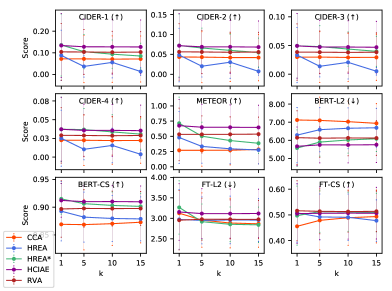
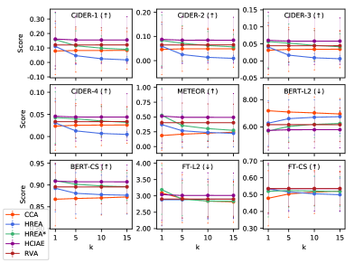
Figure 3: Overlap and embedding distance metrics for $k=1,5,10,15$ generations from sota models on $\mathcal{H}_{v}$ (top) and the full validation set (bottom). cca -aq-g and rva generally show improving trends with increasing $k$, which isn’t the case for hrea-qih-g variants.

6 Discussion

In this paper, we propose a revised evaluation suite for VisDial drawing on existing metrics from the nlp community that measures similarity between answers generated by a model and a given reference set of answers. We arrive at the need for alternate evaluations through the findings of Massiceti et al. (2018) and our own analysis of existing evaluation metrics on the VisDial dataset, which we show can suffer from a number of issues to do with a mismatch between the vd task and an evaluation for it that depends on ranking metrics. While a recent update to the evaluation paradigm of VisDial incorporates both human judgements of answer validity and multiple plausible answers into a final score, issues relating to ranking persist, albeit to a lesser extent. Here, we advocate use of answers directly generated by a model, in concert with consensus-based metrics measuring similarity against sets of answers marked as valid by human annotators.

It is practically infeasible to obtain these validity judgements at scale, however, thus restricting the extent to which the revised scheme can be applied. To address this issue, we develop a semi-supervised automated mechanism to extract sets of relevant answers from given candidate sets, using sparse human annotations and correlations through cca. We verify these sets by computing their intersection with those marked by humans, asking turkers via amt, and measuring their utility for the vd task. Based on such experiments, we expand the VisDial dataset with these reference set annotations and release this and the revised evaluation scheme as DenseVisDial for future evaluation and model development. We intend this to be one possible improvement in the face of inherent constraints on the VisDial dataset, and hope that the community adopts the revised evaluation going forwards.

Acknowledgments This work was supported by ERC grant ERC-2012-AdG 321162-HELIOS, EPSRC grant Seebibyte EP/M013774/1, EPSRC/MURI grant EP/N019474/1, FAIR ParlAI grant, the Skye Foundation and the Toyota Research Institute. We thank Yulei Niu for his help with the rva code.

Appendix A Detailed cca results

We extend the work in Massiceti et al. (2018) and conduct a detailed rank-based performance analysis of cca versus sota approaches across both v0.9 and v1.0 of the VisDial dataset (see Table 5).

Feature extractors

We represent the words in the questions/answers as 300-dimensional FastText (Bojanowski et al., 2017) embeddings. To obtain (300-dimensional) sentence representations, we average word embeddings, following generally received intuition (Arora et al., 2017; Wieting and Kiela, 2019), padding or truncating up to 16 words following Massiceti et al. (2018). While not relevant in the main paper, here we represent images as 512-dimensional pre-trained ResNet34 (He et al., 2016) features, taking the output of conv5, after the avg pool. Our choice of feature extractors is largely arbitrary, however, so to rule out gains from one feature extractor over another and to compare against sota models (Lu et al., 2017; Wu et al., 2018; Das et al., 2017) which use others, we also employ GloVe (Pennington et al., 2014) (300-dimensional, from Common Crawl-42B tokens), and VGG-16/19 (Simonyan and Zisserman, 2015) (4096-dimensional, extracted after the second fc-4096 layer) features for the questions/answers and images, respectively.

Baselines

We compare against ablative versions (without image and/or dialogue history) of the sota models, as well as two nearest-neighbour baselines, as established in (Das et al., 2017):

nn-aq:

given a test question, we find the $k$ nearest-neighbour questions (by average GloVe embedding) from the training set. We take the mean of their $k$ corresponding answers (again in GloVe embedding) to represent a “canonical” answer to that question, ranking the test question’s candidate answers by their $L_{2}$ distances to it.

nn-aqi:

given a test question and image, we first draw the $k$ nearest-neighbour questions to the test question from the training set. From this set, we draw the $k^{\prime}$ questions whose corresponding image features are most similar to the test image feature. Taking the mean of their $k^{\prime}$ corresponding answers, we then rank the test question’s candidate answers as above ($k=100$, $k^{\prime}=20$ as per (Das et al., 2017)).

We also include ncca-aq (no-cca), by computing correlation, as centred cosine distance, directly between the features for questions and answers. Note that for cca -aqi (q), at test time, correlation is computed between questions and candidate answers $\bm{A}$ using projection matrices learned using images (I) as well. Note too that ndcg scores are not computed for v0.9 since human annotations on answer relevance are not available.

Similar to Massiceti et al. (2018), we observe that the mr achieved by cca is similar to that of sota models, despite the approach’s light-weight nature. Comparing to the nearest-neighbour baselines, cca is superior in mr, and additionally in computation and storage requirements since a nearest-neighbour approach requires the train data (including images) at test time.

		Model	I/QA features	MR	R@1	R@5	R@10	MRR	NDCG
sota	v0.9	hciae-g-dis	VGG-19/learned	14.23	44.35	65.28	71.55	0.5467	-
		CoAtt-GAN	VGG-16/learned	14.43	46.10	65.69	71.74	0.5578	-
		hrea-qih-g	”	16.60	42.13	62.44	68.42	0.5238	-
		lf-qih-g	”	16.76	40.86	62.05	68.28	0.5146	-
		hre-qih-g	”	16.97	42.23	62.28	68.11	0.5237	-
		lf-qi-g	”	17.06	42.06	61.65	67.60	0.5206	-
		lf-q-g	”	17.80	39.74	60.67	66.49	0.5048	-
	v1.0	hre-qih-g	VGG-16/learned	18.78	34.78	56.18	63.72	0.4561	0.5245
		lf-qih-g	”	18.81	35.08	55.92	64.02	0.4568	0.5121
		hrea-qih-g	”	19.15	34.73	56.55	63.18	0.4555	0.5189
		mn-qih-g	”	21.25	33.83	54.03	60.65	0.4415	0.5074
		mna-qih-g	”	21.14	34.55	53.57	60.08	0.4451	0.5084
		rva	ResNet101 + rpn/learned	18.50	38.73	57.70	64.73	0.4827	0.5574
Baselines	v0.9	nn-aq	GloVe	19.67	29.88	47.07	55.44	0.3898	-
			FastText	25.92	19.86	34.74	43.55	0.2830	-
		nn-aqi	VGG-16/GloVe	20.14	29.93	46.42	54.76	0.3873	-
			ResNet34/FastText	25.88	21.19	35.78	44.31	0.2941	-
		ncca-aq	FastText	57.18	4.13	9.67	13.89	0.0837	-
cca	v0.9	aq	GloVe	15.86	16.93	44.83	58.44	0.3044	-
			FastText	16.21	16.85	44.96	58.10	0.3041	-
		aqi(q)	ResNet34/FastText	18.27	12.24	35.55	50.88	0.2439	-
			VGG-16/GloVe	26.03	12.24	30.96	42.63	0.2237	-
			VGG-19/GloVe	18.88	12.42	34.52	48.47	0.2409	-
	v1.0	aq	GloVe	16.60	16.10	39.38	54.68	0.2824	0.3504
			FastText	17.07	16.18	40.18	55.35	0.2845	0.3493
		aqi (q)	ResNet34/FastText	19.25	12.63	32.88	48.68	0.2379	0.3077
			VGG-16/GloVe	19.11	13.53	32.43	47.13	0.2415	0.3071
			VGG-19/GloVe	19.29	13.38	32.73	47.23	0.2415	0.3000

Table 5: Results for sota vs. cca on the VisDial v0.9 and v1.0 dataset. cca achieves comparable performance in mean rank (MR) while ignoring both image and dialogue sequence. Note, rpn (Ren et al., 2015).

Appendix B ndcg details

The ndcg is the ratio of the discounted cumulative gain (dcg) of a model’s predicted ranking to the dcg of the ‘ideal’ ranking, obtained by sorting the relevance scores in descending order as $\lx@glossaries@gls@link{acronym}{NDCG}{\leavevmode\textsc{ndcg}}@m=\frac{\lx@glossaries@gls@link{acronym}{DCG}{\leavevmode\textsc{dcg}}@m}{\text{ideal}\>\lx@glossaries@gls@link{acronym}{DCG}{\leavevmode\textsc{dcg}}@m}$, where $m$ is the number of answers with human-derived relevance scores in the set of 100, and $\lx@glossaries@gls@link{acronym}{DCG}{\leavevmode\textsc{dcg}}@m=\sum_{i}^{m}\frac{\rho_{i}}{\log_{2}(i+1)}$. where $i$ is the rank of the answer candidate, and $\rho_{i}$ is the human-assigned relevance score of the $i$-th ranked answer.

Appendix C Full revised evaluation with $H$ and $\Sigma$

Model	cider$\uparrow$				bleu$\uparrow$				meteor$\uparrow$	bert		FastText
	n=1	n=2	n=3	n=4	n=1	n=2	n=3	n=4		$L_{2}$$\downarrow$	CS$\uparrow$	$L_{2}$$\downarrow$	CS$\uparrow$
$A_{\text{gt}}$ $\mu$	0.1889	0.1253	0.0986	0.0819	0.9961	0.4840	0.3934	0.2916	0.9971	5.6087	0.9072	2.6576	0.5681
$\Gamma_{H}$ $\mu$	0.1915	0.1437	0.1165	0.0962	1.0000	0.7633	0.5974	0.3371	1.0000	5.4297	0.9120	2.3339	0.6067
$\sigma$	(0.1490)	(0.1051)	(0.0869)	(0.0772)	(0.0000)	(0.1440)	(0.1538)	(0.1675)	(0.0000)	(1.0121)	(0.0254)	(0.4738)	(0.0850)
$\gamma$	0.2765	0.2151	0.1810	0.1513	1.0000	0.9898	0.9826	0.9300	1.0000	4.7000	0.9334	1.8757	0.6992
cca -aq-g (k=1) $\mu$	0.0721	0.0434	0.0298	0.0226	0.4323	0.1461	0.0345	0.0138	0.2713	7.1231	0.8690	3.1251	0.4555
$\sigma$	(0.1187)	(0.0726)	(0.0506)	(0.0389)	(0.3839)	(0.3189)	(0.1594)	(0.1041)	(0.3083)	(1.7118)	(0.0626)	(0.8266)	(0.1364)
cca -aq-g (k=5) $\mu$	0.0719	0.0431	0.0298	0.0225	0.4195	0.1569	0.0451	0.0131	0.2712	7.1000	0.8685	2.9570	0.4787
$\sigma$	(0.1094)	(0.0640)	(0.0443)	(0.0337)	(0.3169)	(0.2559)	(0.1312)	(0.0592)	(0.2613)	(1.2868)	(0.0455)	(0.6648)	(0.1150)
$\gamma$	0.1108	0.0690	0.0488	0.0373	0.6330	0.3272	0.1275	0.0478	0.4162	6.0801	0.9031	2.5311	0.5571
cca -aq-g (k=10) $\mu$	0.0708	0.0420	0.0291	0.0221	0.4156	0.1539	0.0516	0.0149	0.2721	7.0301	0.8702	2.8850	0.4889
$\sigma$	(0.1071)	(0.0603)	(0.0418)	(0.0317)	(0.2931)	(0.2183)	(0.1248)	(0.0500)	(0.2410)	(1.1316)	(0.0393)	(0.6072)	(0.1077)
$\gamma$	0.1320	0.0840	0.0609	0.0470	0.7251	0.4445	0.2276	0.0960	0.5047	5.7117	0.9132	2.3446	0.5984
cca -aq-g (k=15) $\mu$	0.0715	0.0419	0.0293	0.0222	0.4230	0.1499	0.0585	0.0146	0.2859	6.9386	0.8728	2.8662	0.4935
$\sigma$	(0.1061)	(0.0583)	(0.0402)	(0.0304)	(0.2828)	(0.1873)	(0.1160)	(0.0441)	(0.2375)	(1.0861)	(0.0372)	(0.5732)	(0.1028)
$\gamma$	0.1498	0.0957	0.0704	0.0545	0.7858	0.5191	0.3085	0.1237	0.5908	5.5281	0.9178	2.2542	0.6191
hrea-qih-g (k=1) $\mu$	0.0880	0.0483	0.0333	0.0252	0.5557	0.0948	0.0411	0.0136	0.4813	6.2875	0.8927	2.9724	0.5079
$\sigma$	(0.1161)	(0.0671)	(0.0480)	(0.0374)	(0.4252)	(0.2451)	(0.1799)	(0.1082)	(0.4264)	(1.5281)	(0.0536)	(0.7308)	(0.1146)
hrea-qih-g (k=5) $\mu$	0.0371	0.0202	0.0137	0.0104	0.4343	0.0741	0.0204	0.0048	0.3353	6.5871	0.8820	2.9495	0.4920
$\sigma$	(0.0493)	(0.0269)	(0.0184)	(0.0140)	(0.2975)	(0.1363)	(0.0777)	(0.0400)	(0.2768)	(1.2200)	(0.0450)	(0.5736)	(0.0896)
$\gamma$	0.1171	0.0644	0.0442	0.0335	0.6983	0.1877	0.0596	0.0154	0.5821	5.6691	0.9127	2.5382	0.5625
hrea-qih-g (k=10) $\mu$	0.0558	0.0303	0.0206	0.0156	0.3919	0.0648	0.0169	0.0039	0.2958	6.6661	0.8796	2.9599	0.4907
$\sigma$	(0.0716)	(0.0405)	(0.0290)	(0.0232)	(0.2691)	(0.1190)	(0.0663)	(0.0346)	(0.2452)	(1.1225)	(0.0415)	(0.5827)	(0.0906)
$\gamma$	0.1194	0.0656	0.0450	0.0341	0.7154	0.1975	0.0607	0.0154	0.5915	5.6003	0.9149	2.5639	0.5600
hrea-qih-g (k=15) $\mu$	0.0137	0.0074	0.0051	0.0038	0.3704	0.0606	0.0156	0.0037	0.2767	6.6924	0.8788	2.9571	0.4776
$\sigma$	(0.0178)	(0.0096)	(0.0066)	(0.0050)	(0.2533)	(0.1107)	(0.0619)	(0.0334)	(0.2278)	(1.0705)	(0.0397)	(0.5238)	(0.0809)
$\gamma$	0.1207	0.0663	0.0455	0.0344	0.7227	0.2014	0.0609	0.0154	0.5959	5.5717	0.9158	2.4382	0.5727
hrea-qih-g* (k=1) $\mu$	0.1359	0.0721	0.0494	0.0372	0.7646	0.0614	0.0374	0.0064	0.7149	5.5727	0.9149	3.2664	0.4971
$\sigma$	(0.1431)	(0.0789)	(0.0564)	(0.0430)	(0.4109)	(0.2279)	(0.1875)	(0.0711)	(0.4291)	(1.0037)	(0.0278)	(0.6524)	(0.1148)
hrea-qih-g* (k=5) $\mu$	0.1054	0.0660	0.0480	0.0368	0.6282	0.2607	0.1416	0.0382	0.5027	5.9013	0.9063	2.9186	0.5127
$\sigma$	(0.0791)	(0.0498)	(0.0367)	(0.0282)	(0.2451)	(0.2145)	(0.1688)	(0.0874)	(0.2288)	(0.7756)	(0.0253)	(0.4315)	(0.0808)
$\gamma$	0.2222	0.1472	0.1119	0.0869	0.9582	0.6808	0.4846	0.1623	0.9268	5.0449	0.9274	2.2062	0.6328
hrea-qih-g* (k=10) $\mu$	0.0937	0.0600	0.0438	0.0337	0.5825	0.2739	0.1423	0.0461	0.4310	6.0202	0.9031	2.8534	0.5117
$\sigma$	(0.0656)	(0.0409)	(0.0300)	(0.0231)	(0.2271)	(0.1959)	(0.1412)	(0.0808)	(0.1868)	(0.7250)	(0.0241)	(0.4241)	(0.0761)
$\gamma$	0.2456	0.1701	0.1326	0.1042	0.9780	0.8198	0.6472	0.2946	0.9562	4.9441	0.9295	2.0886	0.6584
hrea-qih-g* (k=15) $\mu$	0.0852	0.0546	0.0398	0.0307	0.5474	0.2635	0.1321	0.0444	0.3866	6.0859	0.9014	2.8411	0.5094
$\sigma$	(0.0591)	(0.0362)	(0.0263)	(0.0202)	(0.2174)	(0.1834)	(0.1265)	(0.0721)	(0.1651)	(0.7063)	(0.0237)	(0.4329)	(0.0750)
$\gamma$	0.2537	0.1793	0.1410	0.1113	0.9815	0.8638	0.7045	0.3525	0.9653	4.8995	0.9305	2.0457	0.6686
mna-qih-g* (k=1) $\mu$	0.1365	0.0713	0.0484	0.0364	0.7713	0.0360	0.0225	0.0019	0.7316	5.5549	0.9153	3.3271	0.4920
$\sigma$	(0.1394)	(0.0767)	(0.0540)	(0.0405)	(0.4134)	(0.1796)	(0.1467)	(0.0333)	(0.4274)	(1.0043)	(0.0279)	(0.6399)	(0.1153)
mna-qih-g* (k=5) $\mu$	0.1066	0.0666	0.0485	0.0370	0.6397	0.2592	0.1485	0.0357	0.5189	5.8719	0.9070	2.9412	0.5104
$\sigma$	(0.0743)	(0.0464)	(0.0344)	(0.0263)	(0.2460)	(0.2148)	(0.1749)	(0.0855)	(0.2298)	(0.7922)	(0.0260)	(0.4207)	(0.0781)
$\gamma$	0.2276	0.1495	0.1137	0.0876	0.9676	0.6748	0.4981	0.1489	0.9425	5.0193	0.9277	2.2086	0.6328
mna-qih-g* (k=10) $\mu$	0.0941	0.0604	0.0443	0.0341	0.5955	0.2786	0.1481	0.0479	0.4483	5.9945	0.9037	2.8828	0.5097
$\sigma$	(0.0598)	(0.0377)	(0.0277)	(0.0214)	(0.2314)	(0.1932)	(0.1398)	(0.0811)	(0.1969)	(0.7360)	(0.0247)	(0.4223)	(0.0744)
$\gamma$	0.2488	0.1731	0.1358	0.1065	0.9805	0.8228	0.6819	0.2986	0.9640	4.9167	0.9298	2.0722	0.6621
mna-qih-g* (k=15) $\mu$	0.0854	0.0551	0.0404	0.0311	0.5590	0.2709	0.1386	0.0472	0.4028	6.0637	0.9019	2.8721	0.5076
$\sigma$	(0.0535)	(0.0333)	(0.0244)	(0.0189)	(0.2206)	(0.1808)	(0.1239)	(0.0740)	(0.1743)	(0.7067)	(0.0239)	(0.4318)	(0.0735)
$\gamma$	0.2585	0.1835	0.1453	0.1147	0.9856	0.8770	0.7516	0.3688	0.9733	4.8716	0.9308	2.0301	0.6718
hciae-g-dis (k=1) $\mu$	0.1338	0.0718	0.0493	0.0372	0.7515	0.0945	0.0513	0.0104	0.6758	5.6690	0.9122	3.1551	0.5049
$\sigma$	(0.1478)	(0.0809)	(0.0564)	(0.0426)	(0.4009)	(0.2627)	(0.2092)	(0.0926)	(0.4291)	(1.0671)	(0.0304)	(0.6940)	(0.1158)
$\gamma$	0.1338	0.0718	0.0493	0.0372	0.7515	0.0945	0.0513	0.0104	0.6758	5.6690	0.9122	3.1551	0.5049
hciae-g-dis (k=5) $\mu$	0.1278	0.0689	0.0473	0.0357	0.7280	0.1015	0.0518	0.0121	0.6501	5.7489	0.9099	3.1158	0.5062
$\sigma$	(0.1274)	(0.0672)	(0.0464)	(0.0350)	(0.3462)	(0.2129)	(0.1559)	(0.0701)	(0.3738)	(0.9951)	(0.0287)	(0.6097)	(0.1028)
$\gamma$	0.1685	0.0944	0.0662	0.0502	0.8672	0.2178	0.1282	0.0348	0.7995	5.4049	0.9192	2.8464	0.5460
hciae-g-dis (k=10) $\mu$	0.1275	0.0689	0.0473	0.0357	0.7290	0.1050	0.0522	0.0122	0.6489	5.7448	0.9101	3.1146	0.5068
$\sigma$	(0.1259)	(0.0665)	(0.0459)	(0.0347)	(0.3403)	(0.2082)	(0.1492)	(0.0654)	(0.3678)	(0.9929)	(0.0286)	(0.6018)	(0.1014)
$\gamma$	0.1782	0.1019	0.0721	0.0549	0.8917	0.2774	0.1653	0.0525	0.8335	5.3337	0.9212	2.7530	0.5616
hciae-g-dis (k=15) $\mu$	0.1270	0.0683	0.0469	0.0354	0.7266	0.1015	0.0516	0.0121	0.6464	5.7557	0.9097	3.1179	0.5065
$\sigma$	(0.1245)	(0.0655)	(0.0451)	(0.0340)	(0.3374)	(0.2010)	(0.1448)	(0.0637)	(0.3635)	(0.9823)	(0.0285)	(0.5934)	(0.1007)
$\gamma$	0.1848	0.1069	0.0763	0.0581	0.9113	0.3150	0.2019	0.0644	0.8556	5.2762	0.9225	2.6875	0.5707
rva (k=1) $\mu$	0.1042	0.0563	0.0385	0.0291	0.6135	0.1001	0.0433	0.0119	0.5328	6.1466	0.8967	2.9543	0.5161
$\sigma$	(0.1311)	(0.0709)	(0.0491)	(0.0371)	(0.4193)	(0.2532)	(0.1884)	(0.0993)	(0.4304)	(1.4871)	(0.0509)	(0.7253)	(0.1170)
rva (k=5) $\mu$	0.1038	0.0560	0.0383	0.0289	0.6088	0.0983	0.0435	0.0112	0.5319	6.1182	0.8977	2.9773	0.5139
$\sigma$	(0.1038)	(0.0542)	(0.0370)	(0.0279)	(0.2939)	(0.1435)	(0.0969)	(0.0453)	(0.3045)	(1.0522)	(0.0338)	(0.5143)	(0.0873)
$\gamma$	0.1777	0.1008	0.0710	0.0540	0.8968	0.3193	0.1727	0.0510	0.8315	5.3013	0.9219	2.4047	0.600
rva (k=10) $\mu$	0.1025	0.0553	0.0379	0.0286	0.6118	0.0997	0.0416	0.0114	0.5333	6.1314	0.8974	2.9757	0.5129
$\sigma$	(0.0964)	(0.0503)	(0.0344)	(0.0259)	(0.2729)	(0.1265)	(0.0815)	(0.0380)	(0.2869)	(0.9821)	(0.0314)	(0.4743)	(0.0803)
$\gamma$	0.1995	0.1180	0.0845	0.0646	0.9450	0.4660	0.2625	0.0887	0.8963	5.1621	0.9253	2.2568	0.6254
rva (k=15) $\mu$	0.1034	0.0559	0.0383	0.0289	0.6147	0.1011	0.0427	0.0124	0.5366	6.1234	0.8976	2.9739	0.5138
$\sigma$	(0.0946)	(0.0492)	(0.0336)	(0.0253)	(0.2652)	(0.1208)	(0.0784)	(0.0383)	(0.2781)	(0.9575)	(0.0305)	(0.4630)	(0.0788)
$\gamma$	0.2110	0.1290	0.0936	0.0722	0.9575	0.5597	0.3335	0.1249	0.9209	5.0983	0.9267	2.1786	0.6389

Table 6: Overlap and embedding distance metrics computed for $k$ generations against the human-annotated reference set $H$ on the validation subset $\mathcal{H}_{v}$. For hrea-qih-g, on average $\sim$6 answers are the empty string, which are excluded from the computation. Metrics marked $\uparrow$ indicate higher values are better, and those marked $\downarrow$ indicate lower values are better. When $k>0$, $k$ answer generations are sampled from the model—$\mu,\sigma,\text{and}\gamma$ are the mean, standard deviation and maximum of the $k$ scores, respectively, averaged over the dataset. Otherwise, 1 answer generation is sampled and the mean $\mu$ is shown.

Model	cider$\uparrow$				bleu$\uparrow$				meteor$\uparrow$	bert		FastText
	n=1	n=2	n=3	n=4	n=1	n=2	n=3	n=4		$L_{2}$$\downarrow$	CS$\uparrow$	$L_{2}$$\downarrow$	CS$\uparrow$
$A_{\text{gt}}$ $\mu$	0.3502	0.2479	0.2004	0.1692	0.9948	0.4827	0.3935	0.2940	0.9955	4.8643	0.9215	2.2155	0.6764
$\Gamma_{H}$ $\mu$	0.3454	0.2734	0.2320	0.1957	1.0000	0.7586	0.6371	0.3816	1.0000	4.8088	0.9220	1.9997	0.6969
$\sigma$	(0.2241)	(0.1906)	(0.1682)	(0.1485)	(0.0000)	(1.4082)	(0.0369)	(0.6757)	(0.1070)	(1.4082)	(0.0369)	(0.6757)	(0.1070)
$\gamma$	0.4212	0.3429	0.2991	0.2583	1.0000	0.9915	0.9767	0.7904	1.0000	4.2891	0.9373	1.6518	0.7614
cca -aq-g (k=1) $\mu$	0.0789	0.0461	0.0313	0.0235	0.3123	0.0752	0.0129	0.0024	0.1864	7.1873	0.8673	3.0908	0.4782
$\sigma$	(0.1634)	(0.1040)	(0.0716)	(0.0544)	(0.3619)	(0.2381)	(0.0962)	(0.0420)	(0.2478)	(1.6917)	(0.0610)	(0.9044)	(0.1639)
cca -aq-g (k=5) $\mu$	0.0824	0.0489	0.0338	0.0255	0.3244	0.1017	0.0283	0.0048	0.2098	7.0948	0.8690	2.9174	0.5036
$\sigma$	(0.1490)	(0.0927)	(0.0645)	(0.0490)	(0.3223)	(0.2113)	(0.0946)	(0.0332)	(0.2355)	(1.3075)	(0.0451)	(0.7324)	(0.1382)
$\gamma$	0.1301	0.0805	0.0567	0.0431	0.4967	0.2220	0.0868	0.0182	0.3321	6.1208	0.9015	2.4655	0.5891
cca -aq-g (k=10) $\mu$	0.0825	0.0489	0.0342	0.0259	0.3280	0.1041	0.0370	0.0074	0.2255	7.0290	0.8704	2.8408	0.5150
$\sigma$	(0.1397)	(0.0850)	(0.0608)	(0.0462)	(0.3142)	(0.1908)	(0.1062)	(0.0342)	(0.2411)	(1.1715)	(0.0393)	(0.6733)	(0.1279)
$\gamma$	0.1617	0.1025	0.0743	0.0571	0.5902	0.3192	0.1663	0.0477	0.4282	5.7403	0.9118	2.2635	0.6349
cca -aq-g (k=15) $\mu$	0.0834	0.0490	0.0345	0.0261	0.3369	0.1009	0.0402	0.0075	0.2431	6.9513	0.8725	2.8181	0.5198
$\sigma$	(0.1295)	(0.0761)	(0.0544)	(0.0413)	(0.3099)	(0.1661)	(0.0963)	(0.0304)	(0.2463)	(1.1312)	(0.0377)	(0.6271)	(0.1188)
$\gamma$	0.1929	0.1240	0.0914	0.0704	0.6572	0.3860	0.2230	0.0647	0.5126	5.5126	0.9172	2.1557	0.6610
hrea-qih-g (k=1) $\mu$	0.1109	0.0597	0.0409	0.0308	0.4521	0.0656	0.0243	0.0058	0.3710	6.2743	0.8924	2.8815	0.5334
$\sigma$	(0.1591)	(0.0909)	(0.0647)	(0.0494)	(0.4281)	(0.2022)	(0.1377)	(0.0672)	(0.4098)	(1.6571)	(0.0540)	(0.7971)	(0.1415)
hrea-qih-g (k=5) $\mu$	0.0468	0.0251	0.0170	0.0128	0.3457	0.0483	0.0119	0.0022	0.2672	6.6069	0.8809	2.8812	0.5154
$\sigma$	(0.0614)	(0.0338)	(0.0233)	(0.0176)	(0.3040)	(0.1102)	(0.0591)	(0.0251)	(0.2738)	(1.3847)	(0.0474)	(0.6355)	(0.1098)
$\gamma$	0.1518	0.0822	0.0560	0.0422	0.5748	0.1257	0.0351	0.0067	0.4644	5.7237	0.9100	2.4585	0.5980
hrea-qih-g (k=10) $\mu$	0.0254	0.0136	0.0092	0.0069	0.3134	0.0432	0.0099	0.0017	0.2387	6.7067	0.8778	2.8971	0.5046
$\sigma$	(0.0324)	(0.0178)	(0.0122)	(0.0092)	(0.2770)	(0.0961)	(0.0493)	(0.0207)	(0.2444)	(1.2885)	(0.0448)	(0.6059)	(0.1029)
$\gamma$	0.1569	0.0850	0.0579	0.0436	0.5901	0.1349	0.0365	0.0068	0.4742	5.6594	0.9119	2.4015	0.6059
hrea-qih-g (k=15) $\mu$	0.0176	0.0094	0.0064	0.0048	0.2962	0.0408	0.0091	0.0016	0.2237	6.7524	0.8765	2.9010	0.4991
$\sigma$	(0.0222)	(0.0122)	(0.0084)	(0.0063)	(0.2621)	(0.0898)	(0.0449)	(0.0194)	(0.2275)	(1.2328)	(0.0433)	(0.5885)	(0.0987)
$\gamma$	0.1590	0.0861	0.0586	0.0442	0.5964	0.1395	0.0372	0.0068	0.4793	5.6348	0.9127	2.3727	0.6096
hrea-qih-g* (k=1) $\mu$	0.1580	0.0835	0.0568	0.0428	0.5923	0.0418	0.0221	0.0047	0.5269	5.7023	0.9097	3.1888	0.5196
$\sigma$	(0.1824)	(0.1048)	(0.0752)	(0.0580)	(0.4656)	(0.1860)	(0.1431)	(0.0631)	(0.4654)	(1.4204)	(0.0399)	(0.7521)	(0.1525)
hrea-qih-g* (k=5) $\mu$	0.1151	0.0717	0.0523	0.0401	0.4643	0.1551	0.0833	0.0249	0.3553	6.0328	0.9017	2.8978	0.5236
$\sigma$	(0.1033)	(0.0727)	(0.0560)	(0.0433)	(0.2839)	(0.1886)	(0.1418)	(0.0741)	(0.2428)	(1.0778)	(0.0344)	(0.5026)	(0.0983)
$\gamma$	0.2775	0.1804	0.1365	0.1062	0.8505	0.4597	0.2952	0.1038	0.7515	5.0467	0.9253	2.1553	0.6626
hrea-qih-g* (k=10) $\mu$	0.0988	0.0624	0.0456	0.0351	0.4225	0.1580	0.0801	0.0264	0.3031	6.1834	0.8978	2.8438	0.5210
$\sigma$	(0.0847)	(0.0579)	(0.0436)	(0.0338)	(0.2609)	(0.1621)	(0.1110)	(0.0634)	(0.1986)	(0.9805)	(0.0326)	(0.4866)	(0.0895)
$\gamma$	0.3105	0.2122	0.1653	0.1302	0.8918	0.6207	0.4368	0.1742	0.7991	4.8802	0.9287	2.0014	0.6934
hrea-qih-g* (k=15) $\mu$	0.0903	0.0570	0.0416	0.0320	0.3966	0.1529	0.0744	0.0248	0.2740	6.2511	0.8961	2.8371	0.5181
$\sigma$	(0.0765)	(0.0511)	(0.0380)	(0.0295)	(0.2483)	(0.1499)	(0.0966)	(0.0556)	(0.1753)	(0.9376)	(0.0316)	(0.4945)	(0.0876)
$\gamma$	0.3288	0.2303	0.1816	0.1440	0.9118	0.6948	0.5110	0.2133	0.8235	4.7952	0.9304	1.9413	0.7067
mna-qih-g* (k=1) $\mu$	0.1515	0.0777	0.0523	0.0393	0.5824	0.0224	0.0117	0.0016	0.5239	5.7056	0.9099	3.2581	0.5119
$\sigma$	(0.1756)	(0.0938)	(0.0649)	(0.0495)	(0.4717)	(0.1386)	(0.1050)	(0.0354)	(0.4697)	(1.4043)	(0.0396)	(0.7169)	(0.1509)
mna-qih-g* (k=5) $\mu$	0.1118	0.0692	0.0506	0.0387	0.4651	0.1483	0.0828	0.0215	0.3610	6.0294	0.9018	2.9351	0.5177
$\sigma$	(0.0985)	(0.0692)	(0.0537)	(0.0413)	(0.2868)	(0.1797)	(0.1411)	(0.0669)	(0.2515)	(1.0884)	(0.0348)	(0.4845)	(0.0972)
$\gamma$	0.2716	0.1762	0.1336	0.1036	0.8460	0.4560	0.2974	0.0919	0.7494	5.0591	0.9249	2.1713	0.6577
mna-qih-g* (k=10) $\mu$	0.0964	0.0610	0.0448	0.0345	0.4281	0.1573	0.0826	0.0269	0.3124	6.1781	0.8978	2.8812	0.5151
$\sigma$	(0.0791)	(0.0547)	(0.0416)	(0.0322)	(0.2663)	(0.1560)	(0.1083)	(0.0606)	(0.2104)	(0.9934)	(0.0330)	(0.4721)	(0.0879)
$\gamma$	0.3049	0.2102	0.1650	0.1305	0.8865	0.6382	0.4658	0.1881	0.7981	4.8802	0.9284	1.9987	0.6921
mna-qih-g* (k=15) $\mu$	0.0875	0.0554	0.0405	0.0312	0.4007	0.1524	0.0765	0.0257	0.2813	6.2491	0.8960	2.8739	0.5125
$\sigma$	(0.0705)	(0.0475)	(0.0356)	(0.0276)	(0.2527)	(0.1424)	(0.0927)	(0.0543)	(0.1858)	(0.9503)	(0.0321)	(0.4770)	(0.0854)
$\gamma$	0.3221	0.2279	0.1813	0.1442	0.9060	0.7126	0.5459	0.2321	0.8216	4.8014	0.9300	1.9410	0.7049
hciae-g-dis (k=1) $\mu$	0.1614	0.0878	0.0605	0.0457	0.5983	0.0730	0.0348	0.0082	0.5138	5.7374	0.9087	3.0389	0.5347
$\sigma$	(0.1859)	(0.1125)	(0.0827)	(0.0644)	(0.4497)	(0.2314)	(0.1716)	(0.0812)	(0.4533)	(1.4411)	(0.0409)	(0.7878)	(0.1508)
$\gamma$	0.1614	0.0878	0.0605	0.0457	0.5983	0.0730	0.0348	0.0082	0.5138	5.7374	0.9087	3.0389	0.5347
hciae-g-dis (k=5) $\mu$	0.1551	0.0845	0.0581	0.0440	0.5791	0.0746	0.0339	0.0083	0.4939	5.7890	0.9073	3.0136	0.5351
$\sigma$	(0.1643)	(0.0966)	(0.0699)	(0.0542)	(0.4043)	(0.1837)	(0.1252)	(0.0582)	(0.4090)	(1.3565)	(0.0388)	(0.6998)	(0.1349)
$\gamma$	0.2063	0.1173	0.0825	0.0629	0.7082	0.1626	0.0863	0.0239	0.6111	5.4373	0.9168	2.7232	0.5840
hciae-g-dis (k=10) $\mu$	0.1551	0.0846	0.0582	0.0440	0.5789	0.0749	0.0338	0.0084	0.4935	5.7920	0.9073	3.0149	0.5349
$\sigma$	(0.1617)	(0.0951)	(0.0686)	(0.0532)	(0.3979)	(0.1773)	(0.1197)	(0.0560)	(0.4032)	(1.3447)	(0.0385)	(0.6881)	(0.1330)
$\gamma$	0.2243	0.1301	0.0924	0.0706	0.7488	0.2083	0.1145	0.0347	0.6480	5.3431	0.9192	2.6187	0.6010
hciae-g-dis (k=15) $\mu$	0.1551	0.0846	0.0582	0.0440	0.5791	0.0750	0.0340	0.0084	0.4931	5.7927	0.9072	3.0142	0.5351
$\sigma$	(0.1607)	(0.0944)	(0.0681)	(0.0528)	(0.3959)	(0.1752)	(0.1172)	(0.0543)	(0.4014)	(1.3402)	(0.0384)	(0.6837)	(0.1323)
$\gamma$	0.2342	0.1377	0.0985	0.0755	0.7679	0.2365	0.1371	0.0428	0.6669	5.2942	0.9204	2.5596	0.6106
rva (k=1) $\mu$	0.1209	0.0650	0.0445	0.0336	0.4850	0.0673	0.0256	0.0066	0.4033	6.1629	0.8956	2.9040	0.5353
$\sigma$	(0.1644)	(0.0941)	(0.0678)	(0.0521)	(0.4378)	(0.2101)	(0.1431)	(0.0722)	(0.4238)	(1.6415)	(0.0527)	(0.7994)	(0.1437)
rva (k=5) $\mu$	0.1207	0.0650	0.0445	0.0336	0.4817	0.0682	0.0269	0.0069	0.4028	6.1633	0.8955	2.9017	0.5358
$\sigma$	(0.1243)	(0.0678)	(0.0475)	(0.0362)	(0.3351)	(0.1266)	(0.0799)	(0.0375)	(0.3314)	(1.3054)	(0.0404)	(0.5718)	(0.1062)
$\gamma$	0.2165	0.1234	0.0868	0.0661	0.7490	0.2239	0.1055	0.0304	0.6422	5.3442	0.9195	2.3333	0.6348
rva (k=10) $\mu$	0.1210	0.0651	0.0446	0.0337	0.4830	0.0682	0.0268	0.0068	0.4032	6.1638	0.8955	2.9009	0.5358
$\sigma$	(0.1185)	(0.0639)	(0.0444)	(0.0338)	(0.3200)	(0.1120)	(0.0664)	(0.0298)	(0.3172)	(1.2562)	(0.0387)	(0.5358)	(0.1000)
$\gamma$	0.2525	0.1496	0.1073	0.0821	0.8163	0.3327	0.1727	0.0528	0.7066	5.1729	0.9236	2.1777	0.6638
rva (k=15) $\mu$	0.1211	0.0652	0.0447	0.0337	0.4826	0.0685	0.0271	0.0070	0.4028	6.1603	0.8956	2.9008	0.5360
$\sigma$	(0.1164)	(0.0626)	(0.0435)	(0.0330)	(0.3142)	(0.1079)	(0.0632)	(0.0275)	(0.3121)	(1.2403)	(0.0380)	(0.5230)	(0.0982)
$\gamma$	0.2709	0.1646	0.1196	0.0919	0.8457	0.4002	0.2239	0.0736	0.7376	5.0869	0.9256	2.1026	0.6778

Table 7: Overlap and embedding distance metrics computed for $k$ generations against the automatic reference sets $\Sigma$ on the entire validation set. For hrea-qih-g, on average $\sim$6 answers are the empty string, which are excluded in computing statistics. Metrics marked $\uparrow$ indicate higher values are better, and those marked $\downarrow$ indicate lower values are better. When $k>0$, $k$ answer generations are sampled from the model—$\mu,\sigma,\text{and}\gamma$ are the mean, standard deviation and maximum of the $k$ scores, respectively, averaged over the dataset. Otherwise, 1 answer generation is sampled and the mean $\mu$ is shown.

In Table 4 in the main paper, we show the performance of models using the revised evaluation scheme. Specifically, we measure the similarity of generated answers against either human-annotated reference sets $H$ (for $\mathcal{H}_{v}$) or automatic reference sets $\Sigma$ (for the entire validation set). We measure similarity using the overlap and embedding distance-based metrics described in the main paper.

In Table 6 and Table 7, we extend this analysis for $H$ and $\Sigma$ respectively, showing the empirical results for an increasing number of $k=\{1,5,10,15\}$ generations sampled from each model. We show the mean $\mu$, standard deviation $\sigma$, and maximum $\gamma$ across the $k$ scores. Note, this is visually presented in Figure 3 in the main paper.

We also include two baselines intended as upper bounds: i) $A_{\text{gt}}$, takes the ground-truth answer to be the generated answer, and ii) $\Gamma_{H}$, cycles through $H$, treating each answer as the generated answer. Since each answer in the set could be a plausible one (as marked by humans), we take the best-case score (minimum score for all except embedding-based $L_{2}$ distance for which we take the maximum), and then average over the dataset.

Appendix D Automatic reference set construction

In our work, we explore different semi-supervised methods for automatically extracting relevant answers from given candidate sets, based on the questions and images. These extracted reference sets are then used to evaluate answer generations for the entire VisDial dataset.

As described in the main paper, we apply cca -aq* to solely those $(Q,A)$ pairs in $\mathcal{H}_{t}$ for which humans scored $\rho(A)>0$, and then compute the correlations $\mathcal{C}$ between $A_{\text{gt}}$ and each $A\in\tilde{\bm{A}}$, where $\tilde{\bm{A}}=\bm{A}\setminus A_{\text{gt}}$. We then explore the following clustering heuristics on $\mathcal{C}$:

Simple:

$\Sigma=\{A:\phi(A_{\text{gt}},A)\in[\mathcal{C}_{\text{max}}-\sigma,\mathcal{C}_{\text{max}}]\}\cup\{A_{\text{gt}}\}$, where $\mathcal{C}_{\text{max}}=\mathrm{max}(\mathcal{C}),\sigma=\mathrm{stdev}(\mathcal{C})$.

Meanshift:

choosing the best-ranked cluster $M^{\prime}$ after running meanshift (Comaniciu and Meer, 2002) on $\mathcal{C}$ to derive $M=M^{\prime}\cup\{A_{\text{gt}}\}$.

Agglomerative:

choosing the best-ranked cluster $G^{\prime}$ after running agglomerative clustering on $\mathcal{C}$, with number of clusters set to 5, to derive $G=G^{\prime}\cup\{A_{\text{gt}}\}$.

Note, each unions the resulting set with $A_{\text{gt}}$.

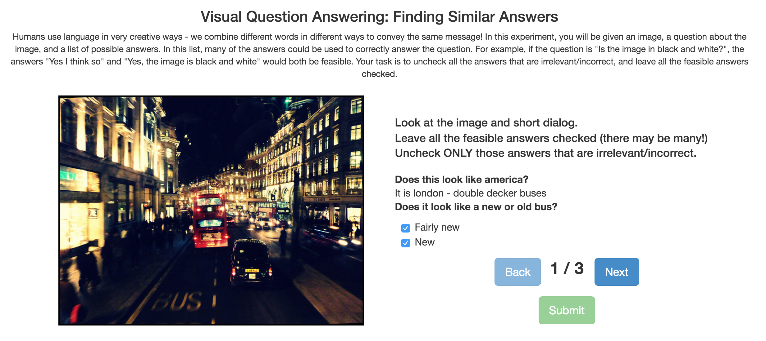
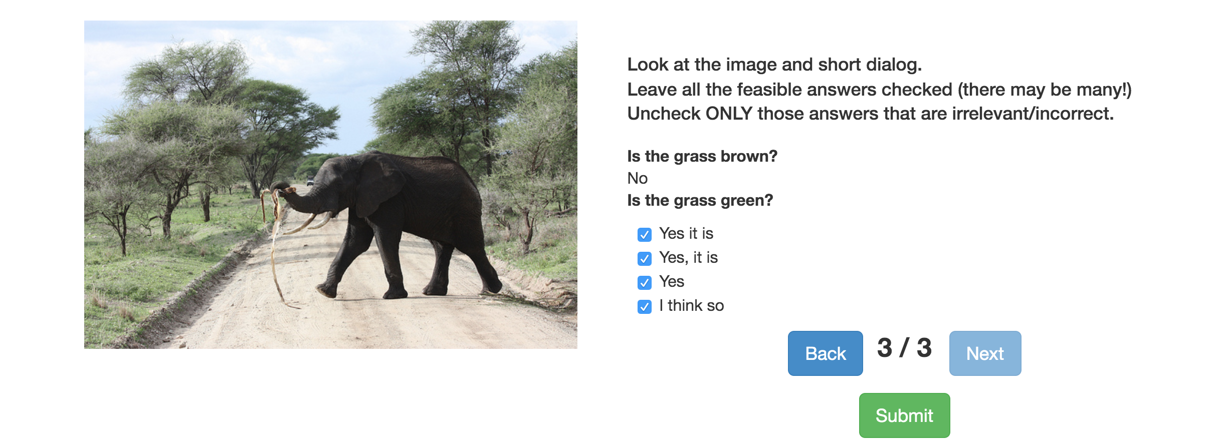
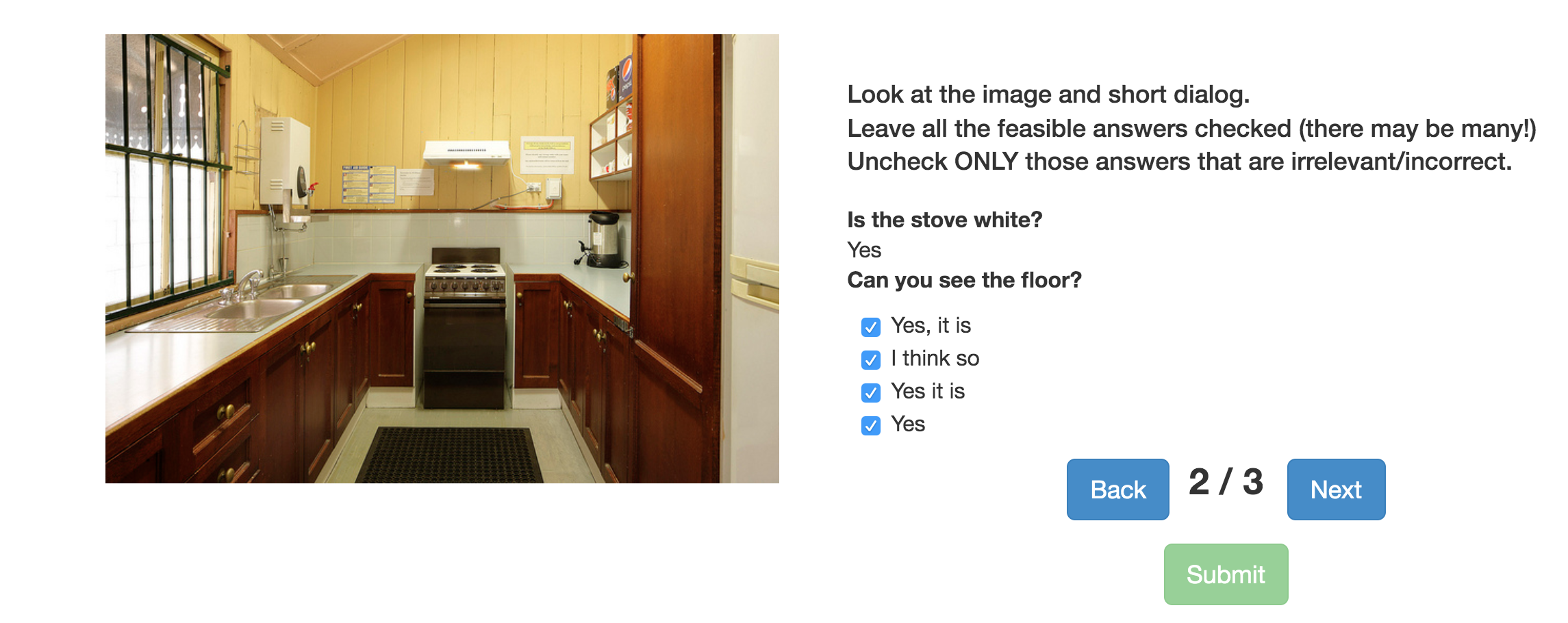
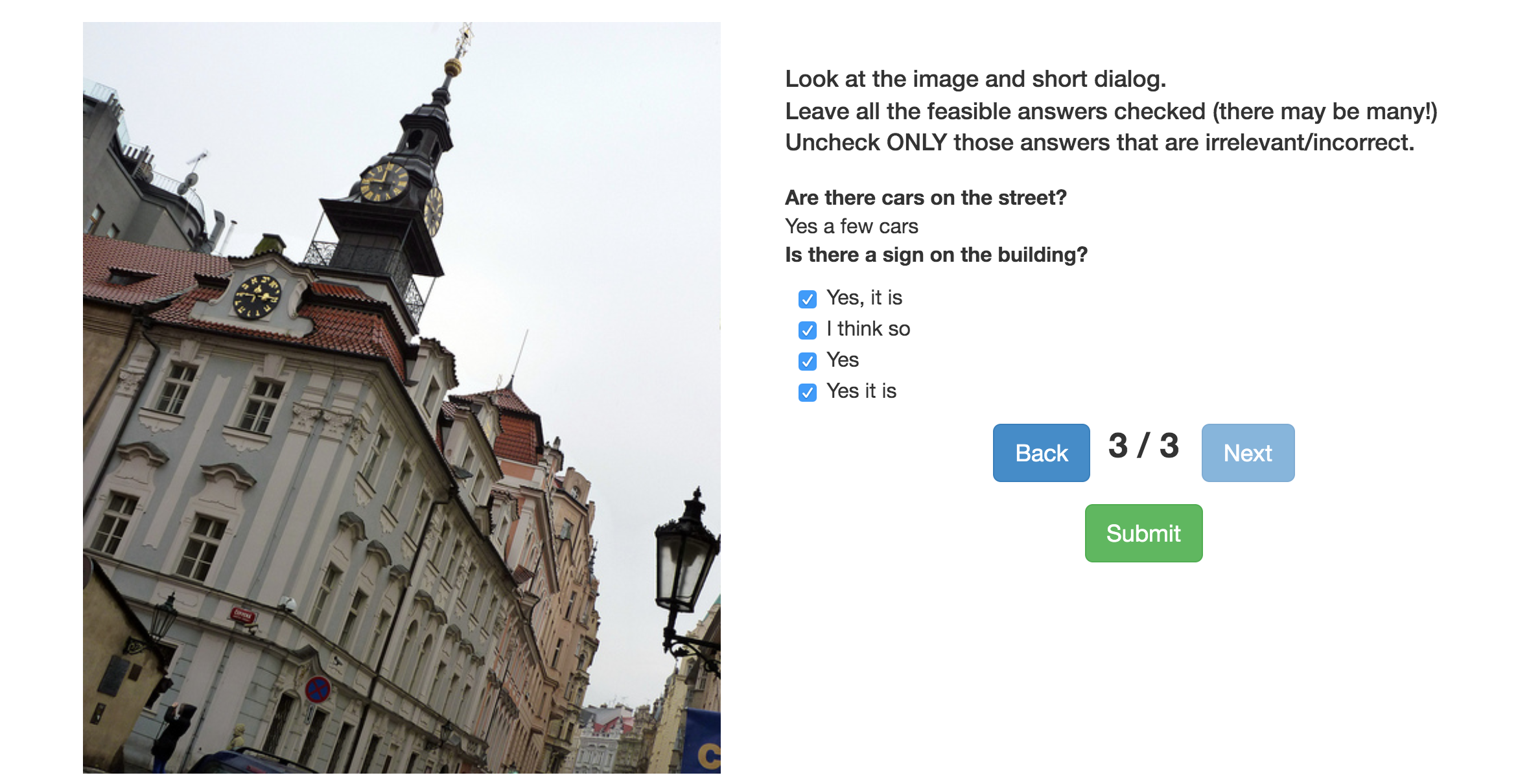
Figure 4: The amt interface we use to verify answer reference sets, sampled from $H$ and $\Sigma$. Turkers are asked to de-select the irrelevant or incorrect answers given an image and question.

Train		Ref	MR	R@1	R@5	R@10	MRR	NDCG
Set	#QA pairs
$\mathcal{H}_{t}$	15,317	$H$	26.49	6.05	21.50	35.53	0.1550	0.3647
	17,055	$\Sigma$	20.36	8.35	32.88	48.78	0.2066	0.3715
	26,318	$M$	21.53	6.83	29.80	45.63	0.1862	0.3503
	16,923	$G\text{ (n=5)}$	20.66	8.08	30.35	46.33	0.1981	0.3657
	1996	$\{A_{\text{gt}}\}$	23.71	13.13	34.05	46.90	0.2428	0.2734
all train	1,232,870	$\{A_{\text{gt}}\}$	17.07	16.18	40.18	55.35	0.2845	0.3493
	10,419,489	$\Sigma$	17.20	10.73	34.20	51.80	0.2312	0.4023
	17,600,151	$M$	20.67	9.38	24.45	39.93	0.1905	0.3339
	10,614,163	$G\text{ (n=5)}$	17.79	9.78	31.40	48.93	0.2171	0.3918
all trainval	1,253,510	$\{A_{\text{gt}}\}$	17.10	16.10	40.05	55.07	0.2833	0.3486
	10,599,533	$\Sigma$	17.31	10.20	33.30	51.45	0.2242	0.4050
	17,931,897	$M$	20.47	9.38	24.83	40.55	0.1917	0.3380
	10,798,877	$G\text{ (n=5)}$	17.60	9.85	31.67	49.20	0.2184	0.3927

Table 8: Extended evaluation of the utility of automatic reference set construction methods ($M,\Sigma,G$) on the standard vd evaluation. Models were trained using cca on the indicated subsets ($\mathcal{H}_{t}$, all train, or all trainval) of VisDial v1.0, using answers drawn from different sets (‘Ref’), and tested on the evaluation test server.

Train		Ref	MR	R@1	R@5	R@10	MRR	NDCG
Set	#QA pairs
$\mathcal{H}_{t}$	15,317	$H$	25.34	6.20	22.58	37.84	0.1598	0.3755
	17,055	$\Sigma$	20.94	8.54	32.16	47.69	0.2049	0.3884
	26,318	$M$	21.84	7.16	28.78	44.95	0.1858	0.3669
	16,923	$G\text{ (n=5)}$	21.47	7.93	30.29	45.89	0.1942	0.3779
	1996	$\{A_{\text{gt}}\}$	23.80	13.50	34.06	46.64	0.2442	0.2816
all train	1,232,870	$\{A_{\text{gt}}\}$	17.04	16.00	41.21	55.16	0.2860	0.3547
	10,419,489	$\Sigma$	17.39	10.27	34.01	51.54	0.2264	0.4099
	17,600,151	$M$	20.96	9.11	22.92	39.30	0.1850	0.3354
	10,614,163	$G\text{ (n=5)}$	18.03	9.68	31.16	48.85	0.2136	0.4005

Table 9: Extended evaluation of the utility of automatic reference set construction methods ($M,\Sigma,G$) on the standard vd evaluation. Models were trained using cca on the indicated subsets ($\mathcal{H}_{t}$, all train, or all trainval) of VisDial v1.0, using answers drawn from different sets (‘Ref’), and tested on the validation set.

D.1 Verifying automatic reference sets

In the main paper, we describe a three-step procedure which we use to verify the quality of the automatic reference sets.

Computing intersection with $H$

Table 10 extends Table 1 in the main paper and shows the iou, precision, recall, and set size for the reference sets extracted by the different methods $C=\{\Sigma,M,G\}$ against $H$—denoted $(A_{\text{gt}},\tilde{\bm{A}})$. Within the reference sets $C$, we also compute the average correlation, the standard deviation of the correlations, and the likelihood of $C$ containing $A_{\text{gt}}$.

In Table 10 we additionally show the results of the above, but using i) cca-aq, learned on all train $(Q,A)$ pairs, and ii) correlations $\mathcal{C}$ computed between $A_{\text{gt}}$ or the question $Q$, and the full candidate set—$(A_{\text{gt}},\bm{A})$ and $(Q,\bm{A})$, respectively. In the case of ($Q,\bm{A}$), we can construct $C$ in two ways: either by selecting all those answers in $\bm{A}$ with the same cluster label as $A_{\text{gt}}$, or those with the same label as the answer with the maximum correlation to $Q$. We denote this $(Q,\bm{A})_{\text{gt}}$ and $(Q,\bm{A})_{\text{max}}$, respectively. This does not apply to $(A_{\text{gt}},\bm{A})$ since $A_{\text{gt}}$ and the answer with the maximum correlation will always be the same, nor for $(A_{\text{gt}},\tilde{\bm{A}})$, since $A_{\text{gt}}$, by definition, is excluded from $\tilde{\bm{A}}$, and simply unioned with the resulting cluster afterwards.

We cross-validate and select the method (in our case, $\Sigma$) which gives us the best precision, $|H\cap C|/|C|$, and a small cluster size, $|C|$. Using this method, we show some qualitative examples of the automatic reference sets $\Sigma$ in Figure 5. The majority of the answers are relevant both to the image and the question.

C			$\frac{|H\cap C|}{|H\cup C|}$	$\frac{|H\cap C|}{|C|}$	$\frac{|H\cap C|}{|H|}$	$|C|$	$A_{\text{gt}}\in C$	corr ($C$)	std (corr($C$))
$H$		——–	100.00 (0.00)	100.00 (0.00)	100.00 (0.00)	12.77 (7.24)	100.00 (0.00)	0.2393 (0.1942)	0.1670 (0.0917)
$M$	cca -aq	$(Q,\bm{A})_{\text{gt}}$	17.59 (13.04)	31.01 (27.31)	57.67 (32.17)	39.85 (31.51)	100.00 (0.00)	0.2998 (0.2610)	0.0856 (0.0374)
		$(Q,\bm{A})_{\text{max}}$	15.06 (14.31)	37.02 (34.72)	38.43 (35.62)	21.53 (26.14)	54.89 (49.77)	0.4794 (0.2379)	0.0852 (0.0424)
		$(A_{\text{gt}},\bm{A})$	13.14 (12.74)	89.10 (26.06)	18.57 (23.21)	4.37 (10.36)	100.00 (0.00)	0.9466 (0.1016)	0.1586 (0.0844)
		$(A_{\text{gt}},\tilde{\bm{A}})$	19.05 (12.65)	42.68 (30.16)	50.47 (35.70)	27.96 (32.01)	100.00 (0.00)	0.5069 (0.2734)	0,2068 (0.0939)
	cca -aq*	$(Q,\bm{A})_{\text{gt}}$	18.66 (14.83)	25.33 (23.22)	62.46 (27.37)	45.89 (28.70)	100.00 (0.00)	0.1843 (0.2146)	0.0735 (0.0360)
		$(Q,\bm{A})_{\text{max}}$	19.89 (16.99)	34.58 (30.69)	49.39 (34.08)	26.74 (25.82)	53.49 (49.89)	0.3270 (0.2186)	0.0710 (0.0367)
		$(A_{\text{gt}},\bm{A})$	13.15 (12.84)	93.96 (20.12)	16.64 (20.51)	3.12 (8.11)	100.00(0.00)	0.9660 (0.0959)	0.1207 (0.0686)
		$(A_{\text{gt}},\tilde{\bm{A}})$	25.01 (18.40)	59.19 (31.55)	39.35 (28.86)	12.00 (16.07)	100.00 (0.00)	0.5841 (0.2167)	0.2231 (0.0990)
$\Sigma$	cca -aq	$(Q,\bm{A})_{\text{gt}}$	19.92 (12.94)	32.64 (26.49)	64.25 (31.71)	39.45 (29.86)	100.00 (0.00)	0.3334 (0.2310)	0.1162 (0.0637)
		$(Q,\bm{A})_{\text{max}}$	14.42 (13.89)	40.72 (35.20)	27.33 (28.47)	11.32 (13.38)	47.14 (49.93)	0.5193 (0.2034)	0.0661 (0.0295)
		$(A_{\text{gt}},\bm{A})$	12.67 (11.97)	89.83 (25.66)	18.17 (22.76)	4.01 (9.08)	100.00 (0.00)	0.9658 (0.0753)	0.0960 (0.0355)
		$(A_{\text{gt}},\tilde{\bm{A}})$	21.16 (13.60)	49.21 (28.34)	38.60 (28.03)	12.30 (12.17)	100.00 (0.00)	0.5859 (0.1898)	0.2092 (0.0949)
	cca -aq*	$(Q,\bm{A})_{\text{gt}}$	21.94 (15.26)	27.31 (22.21)	77.53 (24.32)	50.37 (29.80)	100.00 (0.00)	0.2194 (0.1879)	0.1002 (0.0647)
		$(Q,\bm{A})_{\text{max}}$	19.64 (17.18)	40.95 (33.44)	32.89 (26.85)	11.93 (9.73)	37.02 (48.30)	0.3739 (0.2000)	0.0505 (0.0264)
		$(A_{\text{gt}},\bm{A})$	13.15 (12.89)	93.32 (19.91)	15.49 (17.80)	2.10 (3.72)	100.00 (0.00)	0.9764 (0.0596)	0.0897 (0.0369)
		$(A_{\text{gt}},\tilde{\bm{A}})$	24.13 (16.73)	62.48 (31.24)	32.91 (23.52)	7.17 (6.94)	100.00 (0.00)	0.6206 (0.1773)	0.2269 (0.0975)
$G$	cca -aq	$(Q,\bm{A})_{\text{gt}}$ n=3	19.56 (13.04)	27.14 (21.46)	58.03 (26.41)	33.78 (18.68)	100.00 (0.00)	0.2888 (0.2430)	0.0851 (0.0398)
		$(Q,\bm{A})_{\text{gt}}$ n=4	19.15 (12.81)	31.61 (24.59)	46.77 (25.22)	23.96 (14.68)	100.00 (0.00)	0.3193 (0.2488)	0.0679 (0.0355)
		$(Q,\bm{A})_{\text{gt}}$ n=5	10.49 (6.31)	17.08 (13.61)	28.42 (17.82)	21.25 (8.64)	100.00 (0.00)	0.5656 (0.1375)	0.0287 (0.0100)
		$(Q,\bm{A})_{\text{max}}$ n=4	17.65 (14.16)	36.87 (29.85)	35.27 (27.86)	14.75 (11.63)	57.17 (49.50)	0.4716 (0.2189)	0.0758 (0.0380)
		$(Q,\bm{A})_{\text{max}}$ n=5	9.47 (8.99)	20.73 (24.04)	19.14 (17.22)	14.94 (8.64)	20.78 (40.59)	0.7673 (0.0605)	0.0336 (0.0121)
		$(A_{\text{gt}},\bm{A})$ n=5	15.53 (13.11)	81.47 (29.65)	21.82 (22.55)	4.70 (7.58)	100.00 (0.00)	0.8879 (0.1561)	0.1513 (0.0692)
		$(A_{\text{gt}},\tilde{\bm{A}})$ n=5	22.13 (13.18)	47.40 (27.16)	38.93 (25.76)	11.58 (9.13)	100.00 (0.00)	0.5633 (0.1943)	0.1987 (0.0834)
	cca -aq*	$(Q,\bm{A})_{\text{gt}}$ n=5	10.49 (6.31)	17.08 (13.61)	28.42 (17.82)	21.25 (8.64)	100.00 (0.00)	0.5656 (0.1375)	0.0287 (0.0100)
		$(Q,\bm{A})_{\text{max}}$ n=5	9.47 (8.99)	20.73 (24.04)	19.14 (17.22)	14.94 (8.64)	20.78 (40.59)	0.7673 (0.0605)	0.0336 (0.0121)
		$(A_{\text{gt}},\bm{A})$ n=5	15.34 (14.45)	89.81 (23.18)	18.42 (19.76)	2.74 (4.20)	100.00 (0.00)	0.9342 (0.1189)	0.1369 (0.0672)
		$(A_{\text{gt}},\tilde{\bm{A}})$ n=4	27.74 (19.02)	54.15 (30.33)	42.51 (26.81)	11.08 (8.49)	100.00 (0.00)	0.5290 (0.1968)	0.2123 (0.0721)
		$(A_{\text{gt}},\tilde{\bm{A}})$ n=5	25.59 (17.69)	59.20 (30.71)	35.74 (24.47)	7.91 (6.18)	100.00 (0.00)	0.5874 (0.1892)	0.2188 (0.0877)

Table 10: Intersection verification of semi-supervised methods for automatic reference set construction on the human-annotated validation subset $\mathcal{H}_{v}$, against $H$. Values in parentheses denote standard deviation across the set. For $G$, $n$ is the number of clusters specified for the agglomerative clustering.

Q: Are there any other people? \scalebox{0.6}{GT}⃝ Way in the background \scalebox{0.6}{}⃝ There are few people way off in background \scalebox{0.6}{}⃝ I see a few in the background \scalebox{0.6}{}⃝ There are a few in the background	Q: Is the driver of the truck nearby? \scalebox{0.6}{GT}⃝ I can’t see anyone in the picture \scalebox{0.6}{}⃝ No people \scalebox{0.6}{}⃝ Can’t see anyone else	Q: Is the broccoli raw or cooked? \scalebox{0.6}{GT}⃝ It’s raw. \scalebox{0.6}{}⃝ Raw	Q: Is the mountain large or small? \scalebox{0.6}{GT}⃝ It’s large \scalebox{0.6}{}⃝ Fairly large \scalebox{0.6}{}⃝ It’s medium size \scalebox{0.6}{}⃝ Large \scalebox{0.6}{}⃝ Pretty large \scalebox{0.6}{}⃝ Medium size I would say not small not large \scalebox{0.6}{}⃝ I would say large

Figure 5: Qualitative examples of the relevant answers our semi-supervised approach ($\Sigma$) extracts from given candidate answer sets. Note, we show all answers which our method extracts from the sets.

Using amt

We show the amt interface and examples of automatic reference sets with their corresponding images and questions in Figure 4. Each hit consisted of 4 images, each with a question and its corresponding answer set. Turkers were given $10$ minutes and $\$0.10$ to complete each. Turkers were also required to be based in the us, uk, or Canada (a proxy for English-speaking) and have a hit approval rating of $\geq 90\%$. We randomly sample $1,680$ and $5,040$ image/question/answer sets from $\mathcal{H}_{v}$ and the full validation set, respectively.

Measuring improvement on vd task

Our final verification aims to demonstrate the usefulness of the automatic reference sets for learning the vd task. We show that the cca -aq model, trained with the automatic reference sets rather than the human-annotated sets $H$ achieve equal or better performance on the vd task. We measure performance primarily by the ndcg score. For completeness, we also show performance in the other rank-based metrics. We extend Table 3 in the main paper by showing results for all automated methods ($M,\Sigma,G$) on the validation and test set in Table 8 and Table 9, respectively.

References

- Anand et al. (2018) Ankesh Anand, Eugene Belilovsky, Kyle Kastner, Hugo Larochelle, and Aaron C. Courville. 2018. Blindfold baselines for embodied QA. CoRR, abs/1811.05013.
- Antol et al. (2015) Stanislaw Antol, Aishwarya Agrawal, Jiasen Lu, Margaret Mitchell, Dhruv Batra, C. Lawrence Zitnick, and Devi Parikh. 2015. VQA: Visual Question Answering. In International Conference on Computer Vision (ICCV).
- Arora et al. (2017) Sanjeev Arora, Yingyu Liang, and Tengyu Ma. 2017. A simple but tough-to-beat baseline for sentence embeddings. In International Conference on Learning Representations (ICLR).
- Bach and Jordan (2002) Francis R. Bach and Michael I. Jordan. 2002. Kernel independent component analysis. Journal of Machine Learning Research (JMLR), 3(Jul):1–48.
- Bojanowski et al. (2017) Piotr Bojanowski, Edouard Grave, Armand Joulin, and Tomas Mikolov. 2017. Enriching word vectors with subword information. In Annual Meeting of the Association for Computational Linguistics (ACL).
- Chen et al. (2015) Xinlei Chen, Hao Fang, Tsung-Yi Lin, Ramakrishna Vedantam, Saurabh Gupta, Piotr Dollár, and C. Lawrence Zitnick. 2015. Microsoft COCO captions: Data collection and evaluation server. CoRR, abs/1504.00325.
- Comaniciu and Meer (2002) Dorin Comaniciu and Peter Meer. 2002. Mean shift: A robust approach toward feature space analysis. Transactions on Pattern Analysis and Machine Intelligence (PAMI), (5):603–619.
- Das et al. (2017) Abhishek Das, Satwik Kottur, Khushi Gupta, Avi Singh, Deshraj Yadav, José M.F. Moura, Devi Parikh, and Dhruv Batra. 2017. Visual Dialog. In Conference on Computer Vision and Pattern Recognition (CVPR).
- De Vries et al. (2017) Harm De Vries, Florian Strub, Sarath Chandar, Olivier Pietquin, Hugo Larochelle, and Aaron C. Courville. 2017. GuessWhat?! Visual object discovery through multi-modal dialogue. In Conference on Computer Vision and Pattern Recognition (CVPR).
- Denkowski and Lavie (2014) Michael Denkowski and Alon Lavie. 2014. Meteor universal: Language specific translation evaluation for any target language. In EACL Workshop on Statistical Machine Translation.
- Devlin et al. (2019) Jacob Devlin, Ming-Wei Chang, Kenton Lee, and Kristina Toutanova. 2019. BERT: Pre-training of deep bidirectional transformers for language understanding. In Annual Meeting of the Association for Computational Linguistics (ACL).
- Hardoon et al. (2004) David R. Hardoon, Sandor Szedmak, and John Shawe-Taylor. 2004. Canonical Correlation Analysis: an overview with application to learning methods. Neural Computation, 16(12):2639–2664.
- He et al. (2016) Kaiming He, Xiangyu Zhang, Shaoqing Ren, and Jian Sun. 2016. Deep residual learning for image recognition. In Conference on Computer Vision and Pattern Recognition (CVPR).
- Hodosh et al. (2013) Micah Hodosh, Peter Young, and Julia Hockenmaier. 2013. Framing image description as a ranking task: Data, models and evaluation metrics. Journal of Artificial Intelligence Research, 47:853–899.
- Hotelling (1936) Harold Hotelling. 1936. Relations between two sets of variates. Biometrika.
- Iscen et al. (2019) Ahmet Iscen, Giorgos Tolias, Yannis Avrithis, and Ondrej Chum. 2019. Label propagation for deep semi-supervised learning. In Conference on Computer Vision and Pattern Recognition (CVPR).
- Johnson et al. (2017) Justin Johnson, Bharath Hariharan, Laurens van der Maaten, Li Fei-Fei, C. Lawrence Zitnick, and Ross Girshick. 2017. CLEVR: A diagnostic dataset for compositional language and elementary visual reasoning. In Conference on Computer Vision and Pattern Recognition (CVPR).
- Kettenring (1971) J. R. Kettenring. 1971. Canonical analysis of several sets of variables. Biometrika.
- Lee (2013) Dong-Hyun Lee. 2013. Pseudo-label: The simple and efficient semi-supervised learning method for deep neural networks. In International Conference on Machine Learning (ICML), Workshop on Challenges in Representation Learning.
- Lu et al. (2017) Jiasen Lu, Anitha Kannan, Jianwei Yang, Devi Parikh, and Dhruv Batra. 2017. Best of both worlds: transferring knowledge from discriminative learning to a generative visual dialog model. In Advances in Neural Information Processing Systems (NeurIPS).
- Massiceti et al. (2018) Daniela Massiceti, Puneet K. Dokania, N. Siddharth, and Philip H. S. Torr. 2018. Visual dialogue without vision or dialogue. CoRR, abs/1812.06417.
- Mellish and Dale (1998) Chris Mellish and Robert Dale. 1998. Evaluation in the context of natural language generation. Computer Speech & Language, 12(4):349–373.
- Niu et al. (2019) Yulei Niu, Hanwang Zhang, Manli Zhang, Jianhong Zhang, Zhiwu Lu, and Ji-Rong Wen. 2019. Recursive visual attention in visual dialog. In Conference on Computer Vision and Pattern Recognition (CVPR).
- Pennington et al. (2014) Jeffrey Pennington, Richard Socher, and Christopher D. Manning. 2014. GloVe: Global vectors for word representation. In Conference on Empirical Methods in Natural Language Processing (EMNLP).
- Peters et al. (2018) Matthew E. Peters, Mark Neumann, Mohit Iyyer, Matt Gardner, Christopher Clark, Kenton Lee, and Luke Zettlemoyer. 2018. Deep contextualized word representations. In North American Chapter of the Association for Computational Linguistics (NAACL).
- Reiter and Belz (2009) Ehud Reiter and Anja Belz. 2009. An investigation into the validity of some metrics for automatically evaluating natural language generation systems. Computational Linguistics, 35(4):529–558.
- Ren et al. (2015) Shaoqing Ren, Kaiming He, Ross Girshick, and Jian Sun. 2015. Faster R-CNN: Towards real-time object detection with region proposal networks. In Advances in Neural Information Processing Systems (NeurIPS).
- Sharma et al. (2017) Shikhar Sharma, Layla El Asri, Hannes Schulz, and Jeremie Zumer. 2017. Relevance of unsupervised metrics in task-oriented dialogue for evaluating natural language generation. CoRR, abs/1706.09799.
- Simonyan and Zisserman (2015) Karen Simonyan and Andrew Zisserman. 2015. Very deep convolutional networks for large-scale image recognition. In International Conference on Learning Representations (ICLR).
- Strang et al. (2018) Benjamin Strang, Peter van der Putten, Jan N. van Rijn, and Frank Hutter. 2018. Don’t rule out simple models prematurely: A large scale benchmark comparing linear and non-linear classifiers in OpenML. In International Symposium on Intelligent Data Analysis (IDA), pages 303–315. Springer.
- Vedantam et al. (2015) Ramakrishna Vedantam, C. Lawrence Zitnick, and Devi Parikh. 2015. CIDEr: Consensus-based image description evaluation. In Conference on Computer Vision and Pattern Recognition (CVPR).
- Wieting and Kiela (2019) John Wieting and Douwe Kiela. 2019. No training required: Exploring random encoders for sentence classification. In International Conference on Learning Representations (ICLR).
- Wu and Yap (2006) Kui Wu and Kim-Hui Yap. 2006. Fuzzy SVM for content-based image retrieval: A pseudo-label support vector machine framework. IEEE Computational Intelligence Magazine, 1(2):10–16.
- Wu et al. (2018) Qi Wu, Peng Wang, Chunhua Shen, Ian D. Reid, and Anton van den Hengel. 2018. Are you talking to me? Reasoned visual dialog generation through adversarial learning. In Conference on Computer Vision and Pattern Recognition (CVPR).
- Young et al. (2014) Peter Young, Alice Lai, Micah Hodosh, and Julia Hockenmaier. 2014. From image descriptions to visual denotations: New similarity metrics for semantic inference over event descriptions. Transactions of the Association for Computational Linguistics, 2:67–78.
- Zhou et al. (2015) Bolei Zhou, Yuandong Tian, Sainbayar Sukhbaatar, Arthur Szlam, and Rob Fergus. 2015. Simple baseline for visual question answering. CoRR, abs/1512.02167.