Approximate Approximation on a Quantum Annealer

Abstract.

Many problems of industrial interest are NP-complete, and quickly exhaust resources of computational devices with increasing input sizes. Quantum annealers (QA) are physical devices that aim at this class of problems by exploiting quantum mechanical properties of nature. However, they compete with efficient heuristics and probabilistic or randomised algorithms on classical machines that allow for finding approximate solutions to large NP-complete problems.

While first implementations of QA have become commercially available, their practical benefits are far from fully explored. To the best of our knowledge, approximation techniques have not yet received substantial attention.

In this paper, we explore how problems’ approximate versions of varying degree can be systematically constructed for quantum annealer programs, and how this influences result quality or the handling of larger problem instances on given set of qubits. We illustrate various approximation techniques on both, simulations and real QA hardware, on different seminal problems, and interpret the results to contribute towards a better understanding of the real-world power and limitations of current-state and future quantum computing.

1. Introduction

Many industrial problems belong to complexity class NP, the set of problems solvable with a non-deterministic Turing machine in polynomial time. Even if there are efficient algorithms for small instances using fixed parameter or approximation algorithms (ren19, ; cyg19, ; dev19, ) there are no known algorithms to solve large enough instances exactly and efficiently.

Quantum annealing is one candidate that might solve such hard problems in less time than classical machines. The exact relations between classical and quantum computational power still pose many open questions, despite recent popular results that prove quantum supremacy for certain very specific problems (aru19, ). In particular, it is not expected that quantum computers will be able to solve NP-complete problems in polynomial time (aar13, ).

Industrial use-cases rarely focus on decision problems, but often concern approximate optimisation. For instance, a practical use of the travelling salesperson problem (TSP) is not to ask “is there a closed route of length $n$ between cities?” (which would be captured by the NP-complete decision version of problem) , but rather “what are possible short routes?”, as described by the NPO version. Accepting slight deviations from optimal solutions can lead to substantial savings in temporal effort for many problems, which is usually preferable in pratical applications.

First instances of commercially available QAs have appeared (mcg14, ; cas17, ; fel11, ); expected theoretical and practical applications are numerous including quantum chemistry (str19, ), traffic management (sto19, ), network design (din19, ) or quantum assisted learning (wil19, ). However, the precise benefits of QA caused by the drastic shift in hardware implementation are mostly still unchartered territory (gyo19, ).

In this paper, we discuss how programs for QAs can be designed to find non-optimal solutions to NPO problems, and what gains and losses in terms of various qualities are implied. In classical computation, approximation algorithms usually sacrifice precision for decreased runtime as compared to an exact algorithm. Quantum annealers feature constant computation time by nature of their design (see Section 2), and therefore need to trade other factors in relation to closeness to optimality. There are two major opposing influences on solution quality, as Figure 1 illustrates. First, quality depends how well logical qubits can be mapped to the available physical qubits: Not all physical qubits are interconnected, and interactions between unconnected qubits cause increased distance from solution optimality. Second, exact mathematical formulations lead to perfect solutions on flawless hardware, but complicate the mapping of logical to physical qubits because exact specification usually requires large amounts of qubits. Pruning the problem—for instance by relaxing some of the constraints—is enabled by approximating the problem instance and thus approximating the solution but can also induce opposite effects on real hardware thanks to the smaller amount of required qubits. One of the tasks we address in this work, is to find a balance between an easy mapping of qubits to the hardware, and approximating problems appropriately such that the overall probability of finding good solutions is amplified.

Figure 1. Illustration of solution quality dependent on the embedding’s size (indicated by growing thickness of arrows) and degree of structural approximation (indicated by direction of arrow, whereas up represents good and down bad quality)

2. Basics

Quantum annealing differs considerably from classical notions of algorithmic calculation. Therefore, we briefly summarise the core concepts in this section (readers who wish to remind themselves of the detail can consult standard references like, e.g. (mcg14, ), (nie00, )).

Quantum annealers solve minimisation problems specified as quadratic unconstrained binary optimisation problems (Qubo). A Qubo is a representation of a minimisation formula using binary variables $x_{i}$. For a problem graph $G_{P}=(V,E)$ with nodes $V=\{1,\ldots,n\}$ and weights $c_{i}$ for all nodes and weights $c_{ij}$ for all edges in $E$, the Qubo is defined as (lew17, ) $\min\left(\sum_{i}^{n}c_{i}x_{i}+\sum_{(i,j)\in E}c_{ij}x_{i}x_{j}\right)$. A Qubo can equivalently be specified by all nodes, edges and weights of a problem graph, or by the adjacency matrix of the problem graph. For an introduction on how to formulate a Qubo for a given optimisation problem we refer the reader to (glo18, ).

We perform experiment evaluations on the D-Wave DW2000 Q21 quantum annealer (mcg14, ). Conceptually, the device comprises two components: A processor for solving mathematical problems by quantum mechanical processes, and a user front-end that allows for controlling the processor.

The chip provides about 2000 qubits in the structure of a chimera graph $G_{C}$ (dwa18, ). 16 $\times$ 16 cells are placed in a quadratic grid, and each cell contains a graph with eight nodes. Every node represents a qubit and is connected with four other qubits in the same cell. Different cells are also interconnected, but not on the level of each individual qubit.

To find solutions for a device-independent Qubo $G_{P}$ on the hardware, $G_{P}$ must be mapped to $G_{C}$, referred to as embedding. The limited connectivity of $G_{C}$ with at most six edges per node implies that a node in $G_{P}$ of higher degree cannot directly be embedded, and must be represented by several nodes of $G_{C}$. The amount of qubits requires in $G_{\text{C}}$ is therefore larger than $G_{\text{P}}$, which makes it desirable to formulate problems such that the involved qubits require only low connectivity. For finding a proper embedding we used the tool minorminer by D-Wave Systems Inc.

3. Approximating QUBOs

A fully specified QUBO delivers an exact, optimal solution of the encoded problem if the underlying minimisation problem is solved. A QUBO matrix without non-zero entries does not impose any constraints on the problem variables, and every possible assignment represents a valid solution—in other words, an empty QUBO delivers a set of random binary values as result of an optimisation process.

Interpolating between these scenarios intuitively gives solutions that contain an increasing amount of random choices (and consequently, deteriorating solution quality), while less qubits (non-zero entries in the QUBO) are required to represent the problem. Removing Qubo entries that represent optimisation constraints leads to solutions that are usually not optimal, but valid. Removing entries representing hard constraints often results in invalid solutions. In this context, hard constraints describe all values in a Qubo matrix that represent actual constraints on a solution. If those constraints are violated the solution is not valid and therefore not usable. Consequently, we will focus on problems where most of the Qubo entries are optimisation constraints. Pruning a Qubo induces two contrary effects (cf. Figure 1): Removing entries implies a less exact specification, and decreases solution quality, but sparsely populated Qubo matrices are easier to embed on real QA hardware, which increases solution quality.

We have devised different strategies that produce increasingly approximate versions of a given QUBO:

Fraction:

This methods orders the non-diagonal entries by increasing value. We delete blocks in entries in granularity of 5% of all non-zero values, up to 100%, relative to all entries representing minimisation constraints. We delete small entries first because they are considered to have little effect on the optimal solution and will not approximate the problem instance significantly. Entries representing hard constraints remain in the Qubo, which also holds for the other methods.

Threshold:

This method determines the largest non-diagonal entry. The smallest entry within 5% difference from this value is taken as a threshold. All values below this threshold are pruned from the QUBO. Subsequent approximation steps raise the threshold in increments of 5%.

Random:

This method starts with deleting 5% of randomly chosen Qubo entries (entries representing hard constraints are always kept), and increases the amount of deleted entries to 10%, 15%, etc. for increased degrees of approximation.

Note that eventually, all three methods arrive at identical QUBOs when 100% of the non-hard constraints are purged.

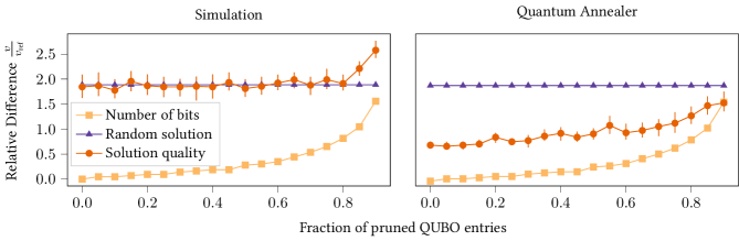
Figure 2. Ratio of errors ($v$) compared to number of elements in set $U$ ($v_{\textrm{ref}}$) and ratio of embed-able instance size ($v$) compared to the original, non-pruned instance ($v_{\textrm{ref}}$) for the Exact Cover Problem

We focus on removing entries representing optimisation constraints. If these occur on non-diagonal entries in the Qubo matrix, deleting leads to reduced connectivity, shorter qubit chains and thus a smaller amount of required physical qubits. However, deleting optimisation constraints from the diagonal of the Qubo matrix while leaving non-diagonal values in the corresponding matrix row or column does not decrease connectivity, and hence does not reduce the amount of required physical qubits. Therefore, we focus on problems where optimisation constraints reside in non-diagonal entries. As all the problems analysed in this paper are computational problems from Karp’s 21 NP-complete problems, the proposed approximation of those problems might not only be of industrial but also scientific interest.

3.1. Exact Cover

The Exact Cover (EC) Problem considers a set $U$ of numbers and a set $V$ of subsets $V_{i}$. An exact cover for $U$ is a collection $V^{\prime}\subset V$ of sets such that every element $u\in U$ appears exactly once in $V^{\prime}$. The decision variant of Exact cover is in NP (kar72, ). One variation of the objective function is to minimize the number of errors: An error occurs if an element of $U$ appears more than once in $V^{\prime}$, or not at all. Following Ref. (luc14, ), the optimisation variant of the exact cover problem is given by

(1) $$\min\sum_{u\in U}\left(1-\sum_{i:u\in V_{i}}x_{i}\right)^{2}$$

The binary variable $x_{i}$ is set $1$ if subset $V_{i}$ is contained in $V^{\prime}$, and $0$ otherwise. A straight-forward reduction from EC to Maximum-Weight Independent Set (MIS) is given by Choi (cho10, ).

To discriminate hardware imperfections from consequences of the approximation proper, we run experiments for each target problem on both, a classical simulation (the dimod.Simulated Annealing Sampler by D-WAVE Systems Inc.) and a quantum annealer. For the EC, our data set requires about 1000 physical qubits to implement the exact Qubo and was pruned step-wise to 53 qubits. Only non-diagonal Qubo entries have been deleted, which represents the information which elements of $U$ appear in which sets $V_{i}$. Every pruned Qubo was solved 100 times. Results are shown in Figure 2. $v/v_{\text{ref}}$ is the relative difference between the number of errors $v$ of the cover compared to a reference value $v_{\textrm{ref}}$, which is the size of set $U$.

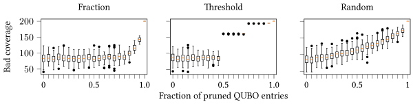
Figure 3. Results for 100 runs of the Exact cover problem on a simulation with different pruning methods

Pruned Qubos require less physical qubits, which in turn means that with increased amounts of pruning, larger problem instances can be embedded on a given amount of physical qubits. Figure 2 also shows the largest size of a pruned instance that can still be represented on the 2048-qubit QA hardware, with the size – in terms of logical qubits – of the unpruned original instance. For the random solution we assigned the 53 logical bits randomly with values 0 and 1 for 100 times. The resulting mean error is also shown in Figure 2. As a random solution is not influenced by the approximation of the problem instance but only the number of logical bits needed, it stays constant throughout the pruning process.

Deleting entries from the Qubo matrix with method fraction results in a constant error for the simulation up to a pruning fraction of about 80%. Removing more than 80% of the Qubo information leads to significantly worse solutions The QA behaves similarly with increasing amount of pruning, save for a lower absolute deviation value from the reference $v_{\textrm{ref}}$. The solution quality is mostly unchanged up to a pruning factor of about 60%, before it decreases significantly. In both cases, the size of embeddable problems increases essentially linearly in the regime of invariant solution quality.

Figure 3 compares the effect of different pruning strategies on the solution (anti-)quality, measured in errors for a cover. The leftmost graph contains the same information as the left-hand part of Figure 2, except that the distribution of results for iterative runs is shown, compared to the mean value on Fig. 2.

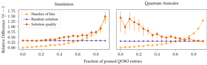
Figure 4. Ratio of solutions ($v$) compared to optimum ($v_{\textrm{ref}}$) and ratio of embeddable instance size ($v$) compared to the original, non-pruned instance ($v_{\textrm{ref}}$) for the Maximum Cut Problem

For the threshold strategy, solution quality remains constant up to a pruning factor of 45% (recall that all values smaller than 45% of the maximal value in the Qubo are deleted in this case). Beyond this regime, solution quality drops considerably.

For strategy random, the solution quality decreases almost linearly with the fraction of pruned Qubo entries. Consequently, method fraction provides the best results even for high pruning factors. Since we observe the same behaviour for the other problems considered in the paper, we restrict our discussion to this pruning strategy in the following.

3.2. Maximum Cut

The Maximum Cut (MC) problem is defined on undirected graphs $G=(V,E)$ and seeks a partition of $V$ into two disjoint sets $V_{1}$, $V_{2}$ such that the cut, that is the number of edges connecting the two sets, is maximal. The decision variant of MC is contained in class NP (kar72, ). Formulating of the MC is straightforward using variable $x_{v}$ that is set 1 if node $v$ is element of $V_{1}$, and 0 otherwise: $\min\sum_{uv\in E}2x_{u}x_{v}-x_{u}-x_{v}$

Figure 4 shows the results of evaluating each pruned Qubo 100 times on a simulation and the QA. The simulation shows a similar behaviour for the size of embeddable instances and solution quality as for the EC. Up to a pruning fraction of 35%, solution quality is almost constant, and up to 70% pruning fraction, only a moderate deterioration in quality can be observed, despite the fact the problem instances comprising up to 50% more logical qubits are tractable.

Compared to a random solution the solution of the simulation is never better. The QA obtains solutions of lower quality even when no pruning has yet been performed. With higher pruning fractions, solutions improve and converge to the solution of a random solution.

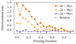
Figure 5. Solution Quality for Maximum Cut for different annealing times and a random solution compared to optimum

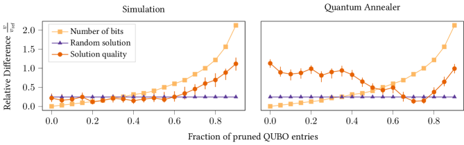
Figure 6. Ratio of solution ($v$) compared to half sum of elements in set $S$ ($v_{\textrm{ref}}$) and ratio of embeddable instance size ($v$) compared to the original, non-pruned instance ($v_{\textrm{ref}}$) for the Number Partitioning Problem

The effect of adjusting physical parameters of the annealer, in particular the annealing time $\Delta t$, is shown in Figure 5. Without any pruning, the standard annealing time of 20$\mu s$ delivers worse solutions than the simulation. Increasing the annealing time to 40$\mu s$ or even 80$\mu s$ provides substantially better solutions especially for less pruned Qubos. With a higher pruning fraction the solutions step-by-step converge to a randomly guessed solution. An optimal value was never reached even with adjusting the annealing time.

3.3. Number Partitioning

The Number Partitioning Problem, one of Karp’s seminal 21 NP-complete problems (kar72, ), asks if a set $S=\{n_{1},...,n_{N}\}$ of numbers can be divided into two subsets $S_{1}$, $S_{2}$ such that $S_{1}\cup S_{2}=S$, $S_{1}\cap S_{2}=\emptyset$ and $\sum_{n_{i}\in S_{1}}n_{i}=\sum_{n_{i}\in S_{2}}n_{i}$. For defining the Number Partitioning problem as an optimisation problem we use the objective function $\min\sum_{n_{i}\in S_{1}}n_{i}-\sum_{n_{i}\in S_{2}}n_{i}$, that is minimising the difference between sets $S_{1}$ and $S_{2}$.

Following (luc14, ), a Qubo formulation of the problem is given by

(2) $$\min A\;\;\left(2\sum_{i=1}^{N}\sum_{j>i}^{N}4x_{i}n_{i}x_{j}n_{j}+\sum_{i=1}^{N}4x_{i}n_{i}^{2}-4k\sum_{i=1}^{N}x_{i}n_{i}+k^{2}\right)$$

with $k=(\sum_{i=1}^{N})^{2}$.

The results of approximating this Qubo by the fraction strategy are shown in Figure 6. Since we minimize the difference between the sum of sets $S_{1}$, $S_{2}$, an optimal solution has got size 0. To define a relative quality measure, we compared the sum $v$ for a given solution to half the sum $v_{\textrm{ref}}$ of all numbers in $S$ by dividing $\frac{v}{v_{\textrm{ref}}}$. For the simulation, deterioration of solution quality and the growing size of the embeddable instances follow the same trend, similar to the simulation of MC. The Quantum Annealer shows a different behaviour: Solutions for the original, non-pruned Qubo are worse on the QA than the same solution on a simulation. Higher pruning fractions lead to better solutions on the QA, also exceeding a randomly guessed solution.

Figure 7 shows the solution quality of runs with different annealing times compared to the half sum of numbers, that have to be partitioned.

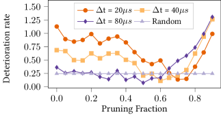
Figure 7. Ratio of solutions to mean sum of numbers in $S$

The solution quality of 100 runs with 20 and 40$\mu s$ are almost identical, thus showing that the adjustment of the annealing time does not change the solution quality for number partitioning. Nevertheless the solutions are mostly worse than the solutions of a simulation. With increasing pruning fraction of more than 80% the quality of solutions drops significantly for all annealing times.

3.4. Airport Gate Assignment Problem

The airport gate assignment problem (AGAP) is a specialisation of the well-known quadratic assignment problem (QAP). It is contained in Apx (sah76, ). For a given airport with $m$ gates and $n$ airplanes, the task is to find an assignment between airplanes and gates so that walk way between gates for passengers changing between flights is minimal (of course, every airplane is assigned to exactly one gate, and no two planes are assigned to the same gate). Related to  (din03, ) this problem is mathematically described by:

$$\min \sum_{i=1}^{n}\sum_{j=1}^{n}\sum_{k=1}^{m}\sum_{l=1}^{m}(p_{i,j}d_{k,l}+a_{i,k})x_{i,k}x_{j,l}+$$

$$\sum_{i=1}^{n}\sum_{k=1}^{m}p_{0,i}d_{0,k}x_{i,k}+\sum_{i=1}^{n}\sum_{k=1}^{m}p_{i,n+1}d_{k,m+1}x_{i,k}+$$

(3) $$A\;\sum_{i}^{n}\left(\sum_{k}^{m}x_{i,k}-1\right)^{2}+B\;\sum_{k}^{m}\left(\sum_{i}^{n}x_{i,k}-1\right)^{2}$$

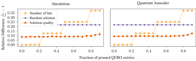
Figure 8. Ratio of solutions ($v$) compared to optimal value ($v_{\textrm{ref}}$) of the instance and ratio of embed-able instance size ($v$) compared to the original, non-pruned instance ($v_{\textrm{ref}}$) for the Airport Gate Assignment Problem.

Figure 9. Ratio of correctly solved clauses ($v$) compared to number of clauses ($v_{\textrm{ref}}$) and ratio of embeddable instance size ($v$) compared to the original, non-pruned instance ($v_{\textrm{ref}}$) for the Maximum 3-SAT Problem

Binary variable $x_{i,k}$ is set 1 if plane $i$ is assigned to gate $k$, and 0 otherwise. $p_{i,j}$ describes the number of passengers changing from plane $i$ to plane $j$ (plane 0 represents a dummy-plane for passengers boarding their initial flight in a multi-leg trip, and dummy-plane $n+1$ collects passengers leaving the airport after their final leg). $d_{k,l}$ specifies the distance between gate $k$ and $l$. Variable $a_{i,k}$ provides costs for assigning plane $i$ to gate $k$. Parameter $y_{i,j}$ describes whether two planes can be assigned to the same gate because they will be on the gate at different times. $A,B\in\mathbb{R}$ are relative weights that ensure that violating a constraint cannot lead to optimal, but incorrect solutions.

Figure 8 shows the result of approximation by pruning, based on 200 runs for each reduced Qubo. In Figure 8 we show the deviation of solutions for simulation and QA calculation compared to the optimal value of the problem instance. Both, QA and simulation, find better solutions than random guessing, and the solution quality is almost constant independent of the degree of approximation. When pruning more than 80% of the Qubo matrix, the solution quality drops to a deviation of 15% from the optimal value. However, using the strongly pruned Qubo, it is possible to embed about 30% larger problems on the quantum hardware.

Problem AGAP is well suited for approximation; since the underlying quadratic assignment problem finds application various industrial relevant contexts, including placement problems, scheduling applications or parallel and distributed computing (cel13, ).

3.5. Maximum 3SAT

Boolean satisfiability with three literals per clause is the cornerstone problem of NP completeness (coo71, ), and the corresponding approximation problem is in the hard approximation class APX (pap91, ). Given a Boolean formula with $n$ variables and $m$ clauses, where each clause contains a disjunction of exactly three literals, the problem is to find an assignment of the $n$ variables that satisfies as many clauses as possible. The decision variant, the 3-SAT Problems, asks whether a given formula can be assigned with $n$ variables such that the whole formula, that is all clauses contained in the formula, is satisfied. Applications of the maximum 3SAT problem are found, for instance, in database systems, combinatorial optimization, or expert systems (che02, ).

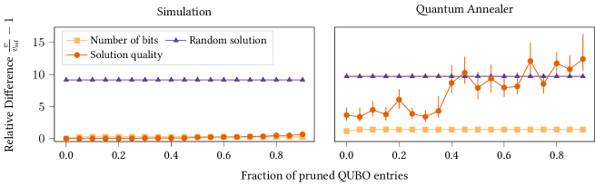
Figure 10. Ratio of solutions ($v$) compared to optimum ($v_{\textrm{ref}}$) and ratio of embeddable instance size ($v$) compared to the original, non-pruned instance ($v_{\textrm{ref}}$) of the travelling salesperson problem.

Following (cho10, ), we obtaining a Qubo for 3SAT via the weighted maximum independent set (WMIS) problem. It is known that for solving randomly created SAT instances, the ratio $\alpha_{c}=m/n$ is an important characteristic quantity that influences the hardness of the problem. For small $\alpha_{c}$, it is on average easy to find a satisfying assignment.

The result of approximation by pruning is shown in Figure 9. Solution quality is mostly invariant for up to 70%. Conflict edges receive larger weights than other edges in the problem graph, and consequently, small Qubo entries are removed first, and conflict edges last. Consequently, the probability of creating a contradiction (where a variable and its negated form are both assigned the same truth value) is small in the initial phase of the pruning process, and the solution quality is stable until entries representing hard constraints are affected.

3.6. Travelling Salesperson

The travelling salesperson problem (TSP) is a well-known NP-complete problem (dur87, ) whose optimisation variant is contained in NPO (aus99, ). An input graph $G=(V,E)$ with $N=\absolutevalue{V}$ and weight $W_{uv}$ for every edge $(u,v)\in E$ and a start node $s$ is given. The TSP seeks a tour through all the nodes, that is, a path $p$ that starts and ends at node $s$, and contains every other node exactly once. The total weight of the path given by $\sum_{(u,v)\in p}W_{uv}$ must be minimised.

Following Lucas (luc14, ), a QUBO for the problem is given by

$$\min\ A\;\sum_{v=1}^{n}(1-\sum_{j=1}^{N}x_{v,j})^{2}+A\;\sum_{j=1}^{n}(1-\sum_{v=1}x_{v,j})^{2}+$$

(4) $$A\;\sum_{(uv)\not\in E}\sum_{j=1}^{N}x_{v,j}x_{v,j+1}+\;\sum_{(uv)\in E}W_{uv}\sum_{j=1}x_{v,j}x_{v,j+1}$$

We use binary variable $x_{v,j}$ to indicate if node $v$ is visited on the $j$-th position in the path. The first two terms in Eq. (4) ensure that every node is visited exactly once within the tour and that there has to be a $j$-th node in the path. The third term prevents that two unconnected nodes appear consecutively in the path; we assume for our analysis that all nodes are connected to each other, and can omit the term. The last term minimises the overall weight of the selected path by adding all weights of the edges contained in the path. Values $A,B$ are positive integers that must satisfy $0<B\max(W_{uv})<A$.

The results of the experiment are given in Figure 10. For the TSP, simulation and QA exhibit completely different behaviour. Up to a pruning fraction of 80%, the solution quality in the simulation is almost invariant. For the QA, solution quality drops considerably after a pruning degree of only 20%. Most importantly, the QA did not obtain any valid solutions, which explains the strong fluctuations in solution quality.

3.7. Graph Coloring

The Graph Coloring problem (GC) is another of Karp’s 21 NP-complete problems (kar72, ). The decision variant of GC decides if the nodes $V$ of a graph $G=(V,E)$ can be colored in such a way that no edge $e\in E$ connects two nodes of the same color. One common objective for an optimisation variant is to minimise the number of required colors. Ref. (kud18, ) solves small instances of GC using a new approach called constrained quantum annealing, which substantially reduces the dimension of the solution space.

For approximate solutions, the number of errors is given by the amount of edges connecting two same-colored nodes. Following (luc14, ), a Qubo formulation of GC is given by

(5) $$\min A\;\sum_{v\in V}(1-\sum_{i=1}^{n}x_{v,i})^{2}+B\;\sum_{uv\in E}\sum_{i=1}^{n}x_{u,i}x_{v,i}$$

Binary variable $x_{v_{i}}$ indicates that node $v$ has color $i$; $n$ gives the number of possible colors. The first term ensures that every node is assigned exactly one color, and the second term minimises the number of errors (ideally, zero).

Running the pruned Qubo 100 times in a simulation and a Quantum annealer gives results as shown in Figure 11. We only delete values that represent the second term of the minimisation formula in 5. The hard constraints that ascertain that assignment of exactly one color to every node remain.

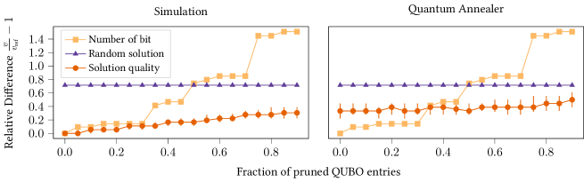
Figure 11. Ratio of errors ($v$) compared to number of nodes in the graph ($v_{\textrm{ref}}$) and ratio of embeddable instance size ($v$) compared to the original, non-pruned instance ($v_{\textrm{ref}}$) for the graph coloring problem.

The simulation shows that approximation leads to only moderate loss in solution quality up to a pruning fraction of 50%, which is desirable. The obtained solutions improve over the random choice baseline. The QA did not find any valid solutions, which means that one node was either assigned two colors, or no color at all.

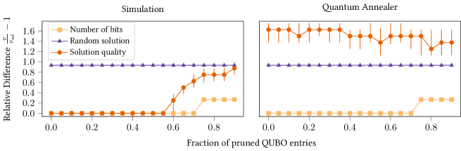
Figure 12. Ratio of errors ($v$) compared to number of nodes in the graph ($v_{\textrm{ref}}$) and ratio of embeddable instance size ($v$) compared to the original, non-pruned instance ($v_{\textrm{ref}}$) for the graph isomorphism problem.

3.8. Graph Isomorphism

Given two graphs $G_{1}=(V_{1},E_{1})$ and $G_{2}=(V_{2},E_{2})$, the graph isomorphism problem (GI) decides if there exists a permutation $P$ such that the adjacency matrices $A_{1}$, $A_{2}$ for graphs $G_{1}$, $G_{2}$ are related by $A_{2}=P^{T}A_{1}P$ (luc14, ). We consider the optimisation variant of the problem, that maximises how many vertices of $G_{1}$ can be mapped onto vertices of $G_{2}$.

Lucas (luc14, ) provides the Qubo formulation

$$\min\ A\;\sum_{v}(1-\sum_{i}x_{v,i})^{2}+A\;\sum_{i}(1-\sum_{v}x_{v,i})^{2}+$$

(6) $$B\;\sum_{(ij)\not\in E_{1}}\sum_{(uv)\in E_{2}}x_{u,i}x_{v,j}+B\;\sum_{(uv)\in E_{1}}\sum_{(uv)\not\in E_{2}}x_{u,i}x_{v,j}$$

Binary variable $x_{v,i}$ is set 1 if node $v$ from $G_{1}$ is mapped to node $i$ from $G_{2}$. The first two terms ensure that every node from $G_{1}$ is assigned to exactly one node from $G_{2}$ and vice versa. The last two terms describe how many edges from one graph cannot be found in the other graph and must be minimised. As the hard constraints consume a substantial portion of the Qubo, the size of the embedding does not decrease significantly with pruning.

The results of 100 simulation and QA runs per pruned Qubo are shown in Figure 12. Similar like for the GC problem, the solutions of simulation and QA clearly differ. While solution quality stays invariant to the pruning of 50% in the simulation, QA could not find any valid solutions at all. Additionally, the growth in size of embeddable instances with increasing pruning fraction is negligible, which makes GI not well suited for approximation.

4. Conclusion

We have introduced several approximation methods for optimisation problems in QUBO formulation that allow us to trade decreasing solution quality for a smaller amount of required qubits. We have compared the behaviour of solution qualities for problems from different approximation complexity classes using a classical simulation and a quantum annealer.

We find that the achievable solution quality on QA is robust against pruning Qubo matrices, often up to pruning ratios as large as 50% or more. Since QAs are probabilistic machines by design, they usually deliver sub-optimal, approximate results anyway, the loss in solution quality is only of subordinate relevance, and is compensated by the fact that pruned Qubo matrices allow for handling larger problem instances on hardware of a given capacity.

We also observe that for many of the problems analysed in this paper, QA without postprocessing delivers solutions that are either close to, or even below the quality of randomly guessed solutions, effectively eliminating any quantum-mechanical advantage. However, as the results obtained by classical simulations show, approximate solutions can—given suitable future hardware—deliver solutions of comparable quality to the full problem description, while remarkably reducing the amount of required qubits. Since the amount of qubits will remain one major limiting factor on real hardware, our results might be useful to enlarge the possible problem sizes treatable on such machines, hopefully assisting first real-world industrial applications of quantum computing.

References

- (1) Aaronson, S.: Quantum Computing since Democritus. Cambridge University Press (2013)
- (2) Arute, F., Arya, K., Babbush, R., et al: Quantum supremacy using a programmable superconducting processor. Nature 574, 505–510 (2019)
- (3) Ausiello, G., Crescenzi, P., Gambosi, G., Kann, V., Marchetti-Spaccamela, A., Protasi, M.: Complexity and Approximation - combinatorial Optimization Problems and their Approximability Properties. Springer-Verlag Berlin (1999)
- (4) van Bevern, R., Tsidulko, O.Y., Zschoche, P.: Fixed-parameter algorithms for maximum-profit facility location under matroid constraints. In: Heggernes, P. (ed.) Algorithms and Complexity. Springer International Publishing (2019)
- (5) Catelvecchi, D.: Quantum cloud goes commercial. Nature (2017)
- (6) Cela, E.: The Quadratic Assignment Problem: Theory and Algorithms. Springer Science and Business Media (2013)
- (7) Chen, J., Kanj, I.A.: Improved exact algorithms for max-sat. In: LATIN 2002: Theoretical Informatics. Springer Berlin Heidelberg (2002)
- (8) Choi, V.: Adiabatic quantum algorithms for the NP-complete maximum weight independent set, exact cover and 3SAT problems. arXiv:1004.2226 (2010)
- (9) Cook, S.A.: The complexity of theorem-proving procedures. Proceedings of the third annual ACM symposium on Theory of computing (1978)
- (10) Cygan, M., Lokshtanov, D., Pilipczuk, M., Pilipczuk, M., Saket, S.: Minimum bisection is fixed-parameter tractable. SIAM J. Comput., 48(2) (2019)
- (11) D-Wave Systems Inc.: Getting started with the D-Wave - User Manual
- (12) Devanur, N.R., Jain, K., Sivan, B., Wilkens, C.A.: Near optimal online algorithms and fast approximation algorithms for resource allocation problems. J. ACM (Jan 2019)
- (13) Ding, H., Lim, A., Rodrigues, B., Zhu, Y.: The airport gate assignment problem. Decision Science Institute Annual Meeting, Washington, DC (2003)
- (14) Ding, Y., Chen, X., Lamata, L., Solano, E., Sanz, M.: Logistic network design with a d-wave quantum annealer (2019)
- (15) Durbin, R., Willshaw, D.: An analogue approach to the travelling salesman problem using an elastic net method. Nature, 326(6114):689 (1987)
- (16) Feldman, M.: D-wave sells first quantum computer. HPCwire (2011)
- (17) Glover, F.W., Kochenberger, G.A.: A tutorial on formulating qubo models. ArXiv abs/1811.11538 (2018)
- (18) Gyongyosi, L., Imre, S.: A survey on quantum computing technology. Computer Science Review(37) (2019)
- (19) Karp, R.: Reducibility among combinatorial problems. Complexity of Computer Computations (1972)
- (20) Kudo, K.: Constrained quantum annealing of graph coloring. Phys. Rev. A 98 (2018)
- (21) Lewis, M.W., Glover, F.: Quadratic unconstrained binary optimization problem preprocessing: Theory and empirical analysis. CoRR (2017)
- (22) Lucas, A.: Ising formulation of many NP-problems. Frontiers in Physics (2014)
- (23) McGeoch, C.: Adiabatic quantum computation and quantum annealing: Theory and practice. Synthesis Lectures on Quantum Computing (2014)
- (24) Nielson, M.A., Chuang, I.L.: Quantum Computation and Quantum Information. Cambridge University Press (2000)
- (25) Papadimitriou, C.H., Yannakakis, M.: Optimization, approximation, and complexity classes. J. Computer and System Sciences 43 (1991)
- (26) Sahni, S.K., Gonzalez, T.F.: P-complete approximation problems. J. ACM 23 (1976)
- (27) Stollenwerk, T., O’Gorman, B., Venturelli, D., Mandrà, S., Rodionova, O., Ng, H., Sridhar, B., Rieffel, E.G., Biswas, R.: Quantum annealing applied to de-conflicting optimal trajectories for air traffic management. IEEE Transactions on Intelligent Transportation Systems (2019)
- (28) Streif, M., Neukart, F., Leib, M.: Solving quantum chemistry problems with a d-wave quantum annealer. In: Feld, S., Linnhoff-Popien, C. (eds.) Quantum Technology and Optimization Problems. Springer International Publishing (2019)
- (29) Venturelli, D., Mandrà, S., Knysh, S., O’Gorman, B., Biswas, R., Smelyanskiy, V.: Quantum optimization of fully connected spin glasses. Physical Review (2015)
- (30) Wilson, M.L., Vandal, T., Hogg, T., Rieffel, E.G.: Quantum-assisted associative adversarial network: Applying quantum annealing in deep learning. ArXiv abs/1904.10573 (2019)