Stability and response of trapped solitary wave solutions of coupled nonlinear Schrödinger equations in an external, $\mathcal{PT}$- and supersymmetric potential

Abstract

We present trapped solitary wave solutions of a coupled nonlinear Schrödinger system in $1$+$1$ dimensions in the presence of an external, supersymmetric and complex $\mathcal{PT}$-symmetric potential. The Schrödinger system this work focuses on possesses exact solutions whose existence, stability, and spatio-temporal dynamics are investigated by means of analytical and numerical methods. Two different variational approximations are considered where the stability and dynamics of the solitary waves are explored in terms of eight and twelve time-dependent collective coordinates. We find regions of stability for specific potential choices as well as analytic expressions for the small oscillation frequencies in the collective coordinate approximation. Our findings are further supported by performing systematic numerical simulations of the nonlinear Schrödinger system.
LA-UR-20-22820

Keywords: $\mathcal{PT}$-symmetric potentials, variational approximation, collective coordinates, dissipation functional, existence and spectral stability analysis.

1 Introduction

The nonlinear Schrödinger equation (NLSE) arises in many areas of physics including Bose-Einstein condensation, plasmas, water waves and nonlinear optics [cNLSreview]. The possibility of experimentally coupling two component NLSE’s in matrix complex potentials has recently been investigated in nonlinear optics situations in which two wave guides are locally coupled through an antisymmetric medium [PhysRevA.99.013823].

On the other hand, $\mathcal{PT}$ symmetry was first introduced into physics as an alternative to Hermiticity in quantum mechanics, yet with real eigenvalues [r:Bender:2007nr, 0305-4470-39-32-E01, 1751-8121-41-24-240301, 1751-8121-45-44-440301]. The similarity of the Schrödinger equation with Maxwell’s equations in the paraxial approximation facilitates the realization of $\mathcal{PT}$ invariant systems in a variety of contexts such as optics [PhysRevLett.100.103904, Makris2011, 0305-4470-38-9-L03, PhysRevLett.101.080402, PhysRevLett.103.123601, PhysRevB.80.235102, PhysRevA.81.022102, r:Ruter:2010mz, PhysRevLett.103.093902, r:Regensburger:2012gf], photonic lattices [SzameitPRA11], electronic circuits [PhysRevA.84.040101, 1751-8121-45-44-444029], mechanical circuits [r:Bender:2013ly], whispering-gallery microcavities [r:Peng:2014ul], among many other physical settings.

Supersymmetry (SUSY) originally considered in high-energy physics to relate fermionic and bosonic systems has also been invoked in condensed matter systems such as fractional quantum Hall states [fqH] and realized in optics [PhysRevLett.110.233902, r:Heinrich:2014qf]. For the Schrödinger equation, supersymmetry relates two potentials which have the same spectrum [r:CooperKhareSukhatmeBOOK, doi:10.1142/S0217751X01004153, Bagchi2000285, Ahmed2001343, PhysRevA.89.032116]. Recently in [1751-8121-50-48-485205], we studied the stability of exact solutions of a single component NLSE in a class of external potentials having SUSY and $\mathcal{PT}$ symmetry.

Our aim in the present work is to extend our considerations to the case of two coupled NLSEs in parity-time or $\mathcal{PT}$-symmetric and supersymmetric external potentials where the cross interaction between the two components is dictated by the nonlinear coupling of the equations. In particular, the superpotential studied in [1751-8121-50-48-485205] is generalized to a matrix form here where we show that it is $\mathcal{PT}$-symmetric. Interestingly, our potential has a non-trivial coupling between the two components which in turn affects the stability of the trapped soliton-like solutions. Our numerical investigations on that front are split into two steps. At first, we will employ a collective coordinate approximation in order to map out the domain of stability of the pertinent waveforms of the coupled system. Then, we will consider the NLSEs and focus on the existence, stability and spatio-temporal evolution of the solitary waves. Upon identifying the steady-state solutions to the NLSEs via fixed-point iterations, we will perform parametric continuations over the parameters of the system. This will allow us to carry out a systematic spectral stability analysis of the solutions and identify parametric regions of stability. Those findings will be corroborated by direct numerical simulations of the NLSEs. Then, we will draw comparisons between the collective coordinate approximation and numerical simulations in regimes where the trapped solutions are stable and unstable. In fact, and in the unstable parametric regime, we will show that the effect of the coupling is responsible for the motion of the solitary waves in opposite directions. Also the amplitudes of the two components respond oppositely to small perturbations.

The structure of the paper is as follows. We discuss the connection to supersymmetry in Sec. 2, and give the exact soliton solutions to the coupled NLSEs in Sec. 3. In Sec. 4 we present the derivation of the equations of motion for the collective coordinate approximation using a variational method which is based on Rayleigh’s dissipation functional. The trial wave functions we have chosen together with the respective dynamic equations for the collective coordinates derived are discussed in Sec. 5. We present results for the dynamical evolution of the collective coordinates in Sec. LABEL:s:dynamicresults where comparisons of these results with numerical simulations are made. In Sec. LABEL:s:CompAnalysis we present numerical results on the existence, stability and dynamics of the exact solutions to the coupled NLSEs. Finally, we state our conclusions in Sec. LABEL:s:Conclusions.

2 Supersymmetry

We consider here a two-component nonlinear Schrödinger (NLS) system in $1$+$1$ (one spatial and one temporal) dimensions of the form:

$$\rmi\,\partial_{t}\Psi(x,t)+\partial_{x}^{2}\Psi(x,t)+\gamma\,[\,\Psi^{{\dagger}}(x,t)\Psi(x,t)\,]\Psi(x,t)-\mathbb{V}(x)\Psi(x,t)=0\>,$$ (2.1)

with

$$\Psi(x,t)=\Biggl{(}\begin{array}[]{c}\psi_{1}(x,t)\\ \psi_{2}(x,t)\end{array}\Biggr{)}\in\mathbb{C}^{2}\>,$$ (2.2)

where $\psi_{j}(x,t)$ is the wave function of the first ($j=1$) and second components ($j=2$), respectively, and $\gamma$ is the nonlinearity strength. The subscripts in Eq. (2.2) stand for differentiation with respect to $t$ and $x$, respectively, and $\left(\cdot\right)^{\dagger}$ corresponds to conjugate transpose.

For a superpotential of the form:

$$\mathbb{W}(x)=r\,\sigma_{0}\,\tanh(x)+\rmi\,s\,\sigma_{3}\,\,\mathrm{sech}(x)\>,$$ (2.3)

where $\sigma_{i}$ are the Pauli matrices, the SUSY partner potentials are given by

$$\mathbb{V}_{\pm}(x) =\mathbb{W}^{2}(x)\pm\partial_{x}\mathbb{W}(x)$$

$$=\sigma_{0}\,r^{2}-\sigma_{0}\,b_{\pm}^{2}\,\mathrm{sech}^{2}(x)+\rmi\,\sigma_{3}\,d_{\pm}\,\mathrm{sech}(x)\tanh(x)\>,$$

where

$$b_{\pm}^{2}=s^{2}+r(r\pm 1)\>,\quad d_{\pm}=s\,(\,2r\mp 1)\>.$$ (2.5)

Note that the partner potentials $\mathbb{V}_{\pm}(x)$ are $\mathcal{PT}$-symmetric.

3 Model potential

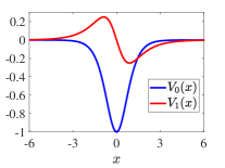
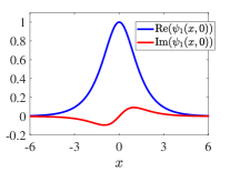
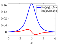
Figure 1: Potential functions and exact solutions are shown in the left, middle and right panels, respectively, for $\gamma=1$, $b=1$, $d=1/2$, and $A_{1}=1$. The value of $A_{2}$ is determined by Eq. (3.8).

The equation we want to solve is (2.1), where the external potential $\mathbb{V}(x)$ is given by

$$\mathbb{V}(x)=\sigma_{0}\,V_{0}(x)+\rmi\,\sigma_{3}\,V_{1}(x)\>.$$ (3.1)

Since we are interested in variational approximations to the moments of the NLSEs, we now show that these equations can be derived from a modified Euler-Lagrange equation by utilizing a Rayleigh dissipation functional. The usual conservative part of the action is

$$\Gamma[\,\Psi^{{\dagger}},\Psi\,]=\!\int\!dt\,\sigma_{0}\,L[\,\Psi^{{\dagger}},\Psi\,],$$ (3.2)

where the conservative part of the Lagrangian $L$ is given by

$$L[\,\Psi^{{\dagger}},\Psi\,]=T[\,\Psi^{{\dagger}},\Psi\,]-H[\,\Psi^{{\dagger}},\Psi\,]\>,$$ (3.3)

with T[ Ψ^†,Ψ ] &= ​∫​dx ⅈ2   {  Ψ^†(x,t) [  ∂_t Ψ(x,t)  ] - [  ∂_t Ψ^†(x,t)  ]   Ψ(x,t)   }  ,
H[ Ψ^†,Ψ ] = ​∫​dx {  —   ∂_x Ψ(x,t)   —^2 - γ2   —  Ψ^†(x,t) Ψ(x,t)  —^2 + V_0(x)   Ψ^†(x,t) Ψ(x,t)   }  . We introduce the dissipation functional $F$ via

$$\mathcal{F}[\,\Psi^{{\dagger}},\Psi;\Psi^{{\dagger}}_{t},\Psi_{t}\,]=\!\int\!dt\,F[\,\Psi^{{\dagger}},\Psi;\Psi^{{\dagger}}_{t},\Psi_{t}\,]$$ (3.4)

where

$$F[\,\Psi^{{\dagger}},\Psi;\Psi^{{\dagger}}_{t},\Psi_{t}\,]=-\rmi\!\int\!dx\,V_{1}(x)\,\Bigl{\{}\,[\,\partial_{t}\Psi^{{\dagger}}(x,t)\,]\,\sigma_{3}\,\Psi(x,t)-\Psi^{{\dagger}}(x,t)\,\sigma_{3}\,[\,\partial_{t}\Psi(x,t)\,]\,\Bigr{\}}\>.$$ (3.5)

The equations of motion for $\Psi(x,t)$ in the presence of a complex potential follow from the generalized Euler-Lagrange equations:

$$\frac{\delta\Gamma[\,\Psi^{{\dagger}},\Psi\,]}{\delta\Psi^{{\dagger}}(x,t)}=-\frac{\delta F[\,\Psi^{{\dagger}},\Psi;\Psi^{{\dagger}}_{t},\Psi_{t}\,]}{\delta\Psi_{t}^{{\dagger}}(x,t)}\>,$$ (3.6)

which lead to the equations of motion

$$\frac{\partial L}{\partial\Psi^{{\dagger}}(x,t)}-\frac{d}{dt}\Bigl{(}\frac{\partial L}{\partial\Psi_{t}(x,t)}\Bigr{)}=-\frac{\partial F}{\partial\Psi_{t}(x,t)}\>,$$ (3.7)

and reproduce Eq. (2.1) with the potential (3.1).

3.1 Exact solution

In component form, Eq. (2.1) reads ⅈ  ∂_tψ_1(x,t) + ∂_x^2ψ_1(x,t) + γ  ( — ψ_1(x,t) —^2+ — ψ_2(x,t) —^2)ψ_1(x,t) - V(x)^∗ψ_1(x,t) &= 0  ,
ⅈ  ∂_tψ_2(x,t) + ∂_x^2ψ_2(x,t) + γ  ( — ψ_1(x,t) —^2+ — ψ_2(x,t) —^2)ψ_2(x,t) - V^∗(x)ψ_2(x,t) = 0  , where $V(x)$ is of the form: $V(x)=V_{0}(x)+\rmi\,V_{1}(x)$, and where we have chosen V_0(x) &= - b^2  sech^2(x)  ,
V_1(x) = - d  sech(x) tanh(x)  . The exact solutions of the system [cf. Eq. (3.1)] are given by ψ_1(x,t) &= A_1  sech(x)   exp{  ⅈ  [  t + ϕ(x)  ]   }  ,
ψ_2(x,t) = A_2  sech(x)   exp{  ⅈ  [  t - ϕ(x)  ]   }  , where $\phi(x)=2d\tan^{-1}[\,\tanh(x/2)\,]$, provided that

$$\gamma\,(\,A_{1}^{2}+A_{2}^{2}\,)=2+(d/3)^{2}-b^{2}\geq 0\>.$$ (3.8)

The left panel of Fig. 1 showcases the potentials $V_{0}(x)$ (solid blue line) and $V_{1}(x)$ (solid red line) whereas the middle and right panels of the figure depict the real (solid blue line) and imaginary (solid red line) parts of the exact solutions $\psi_{1}(x,t)$ and $\psi_{2}(x,t)$ at $t=0$, respectively, for values of the parameters $\gamma=1$, $b=1$, $d=1/2$, and $A_{1}=1$.

4 Collective coordinates (CCs)

In section, we consider two variational approximations for studying the stability and time evolution of the trapped solitary waves. This way, we will be able to compare our findings with numerical simulations of the NLSEs in Sec. LABEL:s:dynamicresults (see, also Sec. LABEL:s:CompAnalysis discussing our computational analysis). We review here the method of collective coordinates, abbreviated CC hereafter (see for example Ref. [1751-8121-50-48-485205]) applied to our case.

The time dependent variational approximation relies on introducing a finite set of time-dependent real parameters in a trial wave function that hopefully captures the time evolution of a perturbed solution. By doing this one obtains a simplified set of ordinary differential equations for the CCs in place of solving the full partial differential equations associated with the NLS system. We begin our discussion by setting

$$\Psi(x,t)\mapsto\tilde{\Psi}[\,x,Q(t)\,]\,,\quad Q(t)=\{\,Q^{1}(t),Q^{2}(t),\dots,Q^{2n}(t)\,\}\in\mathbb{R}^{2n}\>,$$ (4.1)

where $Q(t)$ corresponds to the CCs. It should be pointed out that the success of the method depends greatly on the choice of the trial wave function $\tilde{\Psi}[\,x,Q(t)\,]$. The generalized dissipative Euler-Lagrange equations lead to Hamilton’s equations for $Q(t)$. The Lagrangian in terms of the CCs is given by

$$L(Q,\dot{Q})=T(Q,\dot{Q})-H(Q)\>,$$ (4.2)

where the kinetic term $T(Q,\dot{Q})$ and Hamiltonian $H[\,Q\,]$ are given by

$$T(Q,\dot{Q})=\frac{\rmi}{2}\!\int\!dx\biggl{\{}\,\tilde{\Psi}^{{\dagger}}(x,Q)\,\tilde{\Psi}_{t}(x,Q)-\tilde{\Psi}^{{\dagger}}_{t}(x,Q)\,\tilde{\Psi}(x,Q)\,\biggr{\}}=\pi_{\mu}(Q)\,\dot{Q}^{\mu}\>,$$ (4.3)

and

$$H(Q)=\!\int\!dx\biggl{\{}\,|\partial_{x}\tilde{\Psi}(x,Q)|^{2}-V_{0}(x)\,|\tilde{\Psi}(x,Q)|^{2}-(\gamma/2)\,|\tilde{\Psi}(x,Q)|^{4}\,\biggr{\}}\>,$$ (4.4)

respectively. Note that $\pi_{\mu}(Q)$ in Eq. (4.3) is defined by

$$\pi_{\mu}(Q)=\frac{\rmi}{2}\!\int\!dx\biggl{\{}\,\tilde{\Psi}^{{\dagger}}(x,Q)\,[\,\partial_{\mu}\tilde{\Psi}(x,Q)\,]-[\,\partial_{\mu}\tilde{\Psi}^{{\dagger}}(x,Q)\,]\,\tilde{\Psi}(x,Q)\,\biggr{\}}\>,$$ (4.5)

where we have introduced the notation $\partial_{\mu}\equiv\partial/\partial Q^{\mu}$.

The dissipation functional in terms of the CCs is given by

$$F(Q,\dot{Q})=\rmi\!\int\!dx\,V_{1}(x)\,\biggl{\{}\,\tilde{\Psi}^{{\dagger}}(x,Q)\,\sigma_{3}\tilde{\Psi}_{t}(x,Q)-\tilde{\Psi}_{t}^{{\dagger}}(x,Q)\,\sigma_{3}\tilde{\Psi}(x,Q)\,\biggr{\}}=w_{\mu}(Q)\,\dot{Q}^{\mu}\>,$$ (4.6)

where

$$w_{\mu}(Q)=\rmi\!\int\!dx\,V_{1}(x)\,\biggl{\{}\,\tilde{\Psi}^{{\dagger}}(x,Q)\,\sigma_{3}[\,\partial_{\mu}\tilde{\Psi}(x,Q)\,]-[\,\partial_{\mu}\tilde{\Psi}^{{\dagger}}(x,Q)\,]\,\sigma_{3}\,\tilde{\Psi}(x,Q)\,\biggr{\}}\>.$$ (4.7)

Upon introducing the antisymmetric $2n\times 2n$ symplectic matrix:

$$f_{\mu\nu}(Q)=\partial_{\mu}\pi_{\nu}(Q)-\partial_{\nu}\pi_{\mu}(Q)\,,$$ (4.8)

the generalized Euler-Lagrange equations

$$\frac{\partial L}{\partial Q^{\mu}}-\frac{d}{dt}\Bigl{(}\frac{\partial L}{\partial\dot{Q}^{\mu}}\Bigr{)}=-\frac{\partial F}{\partial\dot{Q}^{\mu}}\>$$ (4.9)

can be written in the form

$$f_{\mu\nu}(Q)\,\dot{Q}^{\nu}=u_{\mu}(Q)=v_{\mu}(Q)-w_{\mu}(Q)\>,$$ (4.10)

by setting $v_{\mu}(Q)=\partial_{\mu}H(Q)$. If $\det\left[{f(Q)}\right]\neq 0$, we can define an inverse as the contra-variant matrix with upper indices:

$$f^{\mu\nu}(Q)\,f_{\nu\sigma}(Q)=\delta^{\mu}_{\sigma}\>,$$ (4.11)

in which case the equations of motion (4.10) can be formulated in the symplectic form:

$$\dot{Q}^{\mu}=f^{\mu\nu}(Q)\,u_{\nu}(Q)\>.$$ (4.12)

We solve this set of equations for our choice of CCs.

5 Trial wave function

We will choose trial wave functions similar to that used for the single-component NLSE in a $\mathcal{PT}$ symmetric complex external potential [1751-8121-50-48-485205]: ~ψ_1[x,Q_1(t)] &= A_1(t)  sech[  β_1(t) (x - q_1(t))  ]   ⅇ^ⅈ  ϕ_1[x,Q_1(t)]  ,
~ψ_2[x,Q_2(t)] = A_2(t)  sech[  β_2(t) (x - q_2(t))  ]   ⅇ^ⅈ  ϕ_2[x,Q_2(t)]  , where ϕ_1[x,Q_1(t)] &= - θ_1(t) + p_1(t)   (x - q_1(t)) + Λ_1(t)   (x - q_1(t))^2 + ϕ(x)  ,
ϕ_2[x,Q_2(t)] = - θ_2(t) + p_2(t)   (x - q_2(t)) + Λ_2(t)   (x - q_2(t))^2 - ϕ(x)  , together with $\phi(x)=(2d/3)\tan^{-1}[\,\tanh(x/2)\,]$. Let us now define

$$M_{i}(t)=\!\int\!dx\,|\psi_{i}(x,t)|^{2}=\frac{|A_{i}(t)|^{2}}{\beta_{i}(t)}\!\int\!dz\,\mathrm{sech}^{2}(z)=\frac{2\,|A_{i}(t)|^{2}}{\beta_{i}(t)}\>,$$ (5.1)

where the integral in the right hand side is calculated in LABEL:s:Integrals (alongside with other integrals useful for the present work).

We consider two sets of variational parameters: Q_1(t) &= {  M_1(t), θ_1(t), q_1(t), p_1(t), β_1(t), Λ_1(t)   }  ,
Q_2(t) = {  M_2(t), θ_2(t), q_2(t), p_2(t), β_2(t), Λ_2(t)   }  , with initial conditions p