VCG Mechanism Design with Unknown Agent Values
under Stochastic Bandit Feedback

Abstract

We study a multi-round welfare-maximising mechanism design problem in instances where agents do not know their values. On each round, a mechanism first assigns an allocation each to a set of agents and charges them a price; at the end of the round, the agents provide (stochastic) feedback to the mechanism for the allocation they received. This setting is motivated by applications in cloud markets and online advertising where an agent may know her value for an allocation only after experiencing it. Therefore, the mechanism needs to explore different allocations for each agent so that it can learn their values, while simultaneously attempting to find the socially optimal set of allocations. Our focus is on truthful and individually rational mechanisms which imitate the classical VCG mechanism in the long run. To that end, we first define three notions of regret for the welfare, the individual utilities of each agent and that of the mechanism. We show that these three terms are interdependent via an $\Omega(T^{\nicefrac{{2}}{{3}}})$ lower bound for the maximum of these three terms after $T$ rounds of allocations, and describe an algorithm which essentially achieves this rate. Our framework also provides flexibility to control the pricing scheme so as to trade-off between the agent and seller regrets. Next, we define asymptotic variants for the truthfulness and individual rationality requirements and provide asymptotic rates to quantify the degree to which both properties are satisfied by the proposed algorithm.

Keywords: Mechanism design, VCG Mechanism, Truthfulness, Game Theory, Bandits

1 Introduction

Mechanism design is one of the most important problems in economics and computer science (Nisan and Ronen, 2001). A mechanism chooses allocations for multiple rational agents with possibly conflicting goals and charges them a price. It is necessary to find an outcome (an allocation to each agent) that is as beneficial as possible to all agents and the mechanism designer. Agents who act in their own self interest might choose to misrepresent their values in order to obtain an advantageous allocation. Mechanism design aims to elicit values from agents, such that the agents are incentivised to report truthfully (truthfulness), while ensuring that they are not worse off than if they had not participated in the mechanism (individual rationality).

As a motivating example, consider a Platform-as-a-Service (PaaS) provider who serves multiple customers using the same compute cluster. The service provider (seller) chooses a service level (allocation) for each customer (agent) and charges them accordingly. The service level determines the resources allocated to the customer, and consequently her value for that service, which could be tied to her own revenue. A customer’s experience of a service level at a given instant is affected by exogenous stochastic factors such as traffic, machine failures, etc., which is beyond the control of the customer. The celebrated VCG mechanism (Vickrey, 1961; Groves, 1979; Clarke, 1971) provides a means to find outcomes which maximise the social welfare (sum of agent and seller utilities) in such situations while satisfying truthfulness and individual rationality. For instance, if one customer’s application is memory intensive and another’s is compute intensive, they can be co-located on the same set of machines instead of using separate machines. This might be a better outcome for the service provider as she can serve both customers at a cheaper cost, and for the customers, since the service provider can now charge them less and they achieve the same end result. The VCG mechanism requires customers to submit bids for each service level and encourages truthful behavior; i.e., the dominant strategy for each customer is to submit their true value as the bid.

A crucial shortcoming of most mechanism design work, which limits its usage in practice, is that it assumes agents know their own values for each allocation. For instance, the VCG mechanism requires that customers submit bids representing these values. This may not be true in many real world situations, especially when there are many unsophisticated agents and/or when the number of allocations is very large. However, having experienced an allocation, it is often the case that a customer can provide feedback based on their experience. She can either measure this directly via the impact on her own revenue, such as in online advertising where an ad impression might lead to a click and then a purchase, or gauge it from performance metrics, such as in the PaaS example where the service level affects the fraction of queries completed on time, which in turn affects her revenue.

Setting: In a departure from prior work, we study mechanisms where agents do not know their values a priori. However, the mechanism can learn them over multiple rounds of allocations and feedback, while simultaneously finding the socially optimal outcome. At the beginning of each round, the mechanism chooses an outcome, i.e. an allocation for each agent, and charges each agent a price. At the end of the round, the agents report stochastic feedback on their experience in using the given allocation, which we will call reward. When choosing an outcome for a given round, the mechanism may use the rewards reported by the agents in previous rounds.

This problem ushers in the classical explore-exploit dilemma encountered in bandit settings. Provided that all agents report their rewards truthfully, choosing the outcome that appears to be the best according to feedback provided by agents up to the current round will likely have large welfare. However, exploring other outcomes might improve the estimate of the best outcome for future rounds.

As is the case in prior mechanism design work, we assume that agents are strategic and rational, which necessitate the truthfulness and individual rationality requirements. A strategic agent wishes to maximise her total utility after $T$ rounds, which is simply the sum of her instantaneous utilities (value of the allocation received minus price). An individually rational agent wishes to ensure that her utility after $T$ rounds is non-negative, so that she stands to gain by participating in the mechanism. Both these requirements are more challenging in our setting. A mechanism cannot learn agent values if she does not report back truthfully. Since she reports a reward at the end of each round, a strategic agent has significantly more opportunity to manipulate outcomes in her favour, than in typical mechanism design settings where she submits a single bid once. In particular, she may be strategic over multiple rounds, say, by incurring losses in early rounds in order to gain in the long run. Additionally, since an agent’s true values cannot be exactly known, the mechanism runs the risk of overcharging them, which might cause her to withdraw from the mechanism.

We design an algorithm that accounts for the above considerations. Applications such as PaaS or online advertising, where there are repeated agent-mechanism interactions and where values can be reported back in an automated way, are suitable for such methods.

	Truthfulness $\mathbb{E}[U^{\pi}_{iT}-U_{iT}]\in\tilde{\mathcal{O}}(\textrm{?})$ (Theorem 2)	Individual rationality $-\mathbb{E}[U_{iT}]\in\tilde{\mathcal{O}}(\textrm{?})$ (Theorem 3)	VCG regret $\mathbb{E}[R^{\rm{\tiny VCG}}_{T}]\in\tilde{\mathcal{O}}(\textrm{?})$ (Theorem 4)
$\zeta={\text{\scriptsize{ETC}}}$	$K^{\nicefrac{{1}}{{3}}}T^{\nicefrac{{2}}{{3}}}$	$n^{\star}(\lambda)K^{\nicefrac{{1}}{{3}}}T^{\nicefrac{{2}}{{3}}}$	$n^{2}K^{\nicefrac{{1}}{{3}}}T^{\nicefrac{{2}}{{3}}}$
$\zeta={\text{\scriptsize{OPT}}}$	$nK^{\nicefrac{{1}}{{3}}}T^{\nicefrac{{2}}{{3}}}$, NIC	$n^{\star}(\lambda)|{\mathcal{S}}|^{\nicefrac{{1}}{{2}}}T^{\nicefrac{{1}}{{2}}}$	$n^{2}K^{\nicefrac{{1}}{{3}}}T^{\nicefrac{{2}}{{3}}}$

Table 1: Summary of asymptotic rates for Algorithm 1 for truthfulness, individual rationality, and the VCG regret $R^{\rm{\tiny VCG}}_{T}$ (3). Above, $n$ denotes the number of agents, $T$ the number of rounds, $|{\mathcal{S}}|$ the number of different allocations, $K$ is a problem-specific parameter defined in Section 3, $U_{iT}$ is the total utility of agent $i$ after $T$ rounds when being truthful, and $U^{\pi}_{iT}$ is the total utility of agent $i$ after $T$ rounds when following any other (non-truthful) strategy $\pi$. Algorithm 1 has two (binary) hyperparameters $\zeta\in\{{\text{\scriptsize{ETC}}},{\text{\scriptsize{OPT}}}\}$, and $\lambda\in\{{\text{\scriptsize{AGE}}},{\text{\scriptsize{SEL}}}\}$, defined in Section 5. While the VCG regret and asymptotic truthfulness rates do not depend on $\lambda$, the rates for asymptotic individual rationality do, via the $n^{\star}$ term, where, we have $n^{\star}({\text{\scriptsize{AGE}}})=1$ and $n^{\star}({\text{\scriptsize{SEL}}})=n$. NIC indicates that the mechanism is asymptotically Nash incentive-compatible. When $\zeta={\text{\scriptsize{ETC}}}$, we have better truthfulness guarantees, but weak rates for individual rationality, and vice versa when $\zeta={\text{\scriptsize{OPT}}}$.

Our Contributions:

Our contribution in this work is threefold:

1. First, we formalise mechanism design with bandit feedback for settings where agents do not know their values, but the mechanism is repeated for several rounds. In order to quantify how close the mechanism is to the VCG mechanism, our formalism defines the VCG regret; this is derived via regret terms for the welfare, the seller, and the agents relative to the VCG mechanism. Additionally, given the above challenges in achieving truthfulness and individual rationality exactly, we define asymptotic variants to make the problem tractable.

2. Second, we establish a hardness result via a $\Omega(T^{\nicefrac{{2}}{{3}}})$ lower bound after $T$ rounds for the VCG regret even under truthful reporting from agents.

3. Third, we describe VCG-Learn, an algorithm whose behaviour is determined by two binary hyperparameters. For all values of these hyperparameters, the algorithm is asymptotically individually rational and truthful, and moreover match the above lower bound on the VCG regret up to factors that are polylogarithmic in $T$ and polynomial in other problem-dependent terms. However, the asymptotic rates and the regrets of the agent and the seller are affected by the choice of these hyperparameters. Table 1 summarises the results for Algorithm 1.

This manuscript is organised as follows. First, in Section 2, we discuss related work. In Section 3, we briefly review the VCG mechanism and describe our formalism. Section 4 presents the lower bound on the VCG regret. Section 5 present our algorithm, VCG-Learn, and Section 6 presents the theoretical results for VCG-Learn. Section 7 presents some simulation results. The proof of the lower bound is given in Section 8 and the proofs of results in Section 6 are given in Section 9.

2 Related Work

Bandit problems were first studied by Thompson (1933) and have since become an attractive framework to study exploration-exploitation trade-offs that arise in online decision-making. Optimistic methods, which usually choose an arm on a given round by maximising an upper confidence bound on the mean rewards, are known to be minimax optimal in a variety of stochastic optimisation settings (Lai and Robbins, 1985; Auer, 2003; Bubeck et al., 2011). Explore-then-commit strategies use separate rounds for exploration and exploitation. While they are provably sub-optimal (Garivier et al., 2016), they separate exploration from exploitation facilitating a cleaner analysis when we need to combine optimisation with other side objectives, such as in our problem, where we need to provide truthfulness guarantees and compute the prices.

Mechanism design has historically been one of the core areas of research in the economics and game theory literature with applications in kidney exchange (Roth et al., 2004), matching markets (Roth, 1986), and fair division (Procaccia, 2013). Our work is on auction-like settings for mechanism design. In addition to a rich history of research on this topic, there has also been a recent flurry of work due to the rise in popularity of sponsored search markets (Lahaie et al., 2007; Mehta et al., 2007; Aggarwal et al., 2006), wireless spectrum auctions (Cramton, 2013; Milgrom, 2017), and cloud spot markets (Toosi et al., 2016).

There is a long history of work in the intersection of machine learning and mechanism design. Some examples include online learning formulations (Dudik et al., 2017; Amin et al., 2013; Kakade et al., 2010), learning bidder values from past observations (Balcan et al., 2016; Blum et al., 2015; Balcan et al., 2008), and learning in other settings with truthfulness constraints (Mansour et al., 2015). Some work in this space study settings where individual agents may learn to bid in a repeated auction. Here, an agent may not know her value at the beginning, but needs to submit bids at the beginning of each round. The agent may calibrate her bid based on past rewards. In this line of work, Weed et al. (2016) and Feng et al. (2018) study a setting where the behaviour of the mechanism is fixed over multiple rounds, while Nedelec et al. (2019) study a setting where the mechanism may adapt its behaviour so as to maximize revenue. In a similar vein,  Liu et al. (2019) develop bandit methods where agents on one side of a matching market learn to bid for arms on the other side. In the above work, the regret is defined for the agent in question, defined relative to an oracle which knows the true values. In contrast to these works, in our setting, learning happens entirely on the mechanism side and the role of each agent is very simple: submit the reward at the end of the round. This imposes minimal burden on agents who, while being strategic and rational, may not be very sophisticated.

A body of work study multi-armed bandit formalisms for auctions with canonical use cases in online advertising (Babaioff et al., 2015, 2014; Devanur and Kakade, 2009). In the above works, there is a single item (ad slot) with different and unknown click-through rates for each agent $c_{i}\in\mathbb{R}$. The agent has a known private value $v_{i}\in\mathbb{R}$ for each click and she submits a bid $b_{i}\in\mathbb{R}$ once ahead of time representing this value. On each round, the mechanism chooses one of the agents for the slot and observes the number of clicks $c$; if agent $i$ was chosen, then $\mathbb{E}[c]=c_{i}$ The agent’s reward for this round is $c\cdot v_{i}$. They formalise this problem where the agents are viewed as the arms and define regret with respect to the optimal arm, i.e. the agent with the highest expected reward $v_{i}\times c_{i}$. Importantly, the stochastic component $c$ of the reward is observed by both the agent and the mechanism. In both works, truthfulness means that the agent is incentivised to submit a bid $b_{i}=v_{i}$ at the beginning of all rounds. There are a number of differences between these works and our setting. First, while they formalise each agent as a different arm competing for the item, in our setting, the allocations are viewed as arms with multiple agents being able to experience different arms simultaneously. We do not believe their results, and their lower bound in particular, can be straightforwardly extended to settings where multiple agents might receive an allocation. Second, in these works the agent can only submit a single bid and the stochastic component of the reward (number of clicks) is observed by the mechanism on each round. In contrast, in our setting, the reward on each round is only revealed to the agent, and she may misreport this reward to the mechanism on each round; therefore, she has significantly more opportunity to manipulate outcomes in her favour. Due to these differences, their results are not comparable to ours. We will elaborate in other differences between our results and theirs in further detail at the end of Sections 4 and 6.

In other related work, Braverman et al. (2019) consider a setting where a seller chooses one of $n$ agents to receive an item on each round of a repeated auction. The agents submit a payment at the end of the round to the seller based on the reward they observed. They study mechanisms that allow the seller to extract as much payment as possible from the agents who themselves are trying to maximise their long term utility.  Nazerzadeh et al. (2016) study a multi-round setting where the seller chooses an agent and a price on each round; the agent may choose to purchase the item at the price in which case the seller receives some revenue. Their goal is to maximise the revenue for the seller over a finite horizon of $T$ rounds.  Gatti et al. (2012) study an online advertising setting when there are multiple ad slots with different click-through rates which are the same for all agents, and design a mechanism which charges the agents only when an ad is clicked. Finally, some work on dynamic auctions (Bergemann and Valimaki, 2006; Athey and Segal, 2013; Kakade et al., 2013) study settings where agent values are unknown at the beginning but there is a known prior on the agent value. Over time, she receives side information and the mechanism needs to incentivise truth telling so as to update the posterior.

Perhaps the closest work to ours is Nazerzadeh et al. (2008), who study a single item auction with a feedback method similar to ours: agents report rewards at the end of the round and the learning happens at the mechanism. While they consider asymptotic efficiency, truthfulness, and individual rationality (with definitions that differ from ours), they do not provide rates, establish lower bounds, or study the regrets of the agents and seller.

3 Problem Description

3.1 A brief review of the VCG mechanism

We begin with a brief review of mechanism design adapted to our setting. There are $n$ agents (customers) $\{1,\dots,n\}$, a mechanism (seller), and a set of possible outcomes $\Omega$. The mechanism chooses an outcome $\omega\in\Omega$ and charges a price $p_{i}$ to each agent. For agent $i$, there exists a function $s_{i}:\Omega\rightarrow{\mathcal{S}}$ which maps outcomes to allocations relevant to the agent; i.e., different outcomes $\omega,\omega^{\prime}$ might yield the same allocation to the agent, $s_{i}(\omega)=s_{i}(\omega^{\prime})$. In this work, $|{\mathcal{S}}|<\infty$. ${\mathcal{S}}$ could be as large as $\Omega$, but could be much smaller in some applications. This distinction between ${\mathcal{S}}$ and $\Omega$ will be important when we consider the learning problem in Section 3.2; as we will see shortly, our regret bounds will scale with $|{\mathcal{S}}|$ and not $|\Omega|$.

Agent $i$ has a value function, $v_{i}:{\mathcal{S}}\rightarrow[0,1]$, where $v_{i}(s)$ represents her private independent value for the allocation $s$. For an outcome $\omega\in\Omega$, we will overload notation and write $v_{i}(\omega)=v_{i}(s_{i}(\omega))$. After the agent experiences an allocation, she realises a reward $X_{i}$ drawn from a $\sigma$ sub-Gaussian distribution with mean $v_{i}(s)$. We let $v_{0}:\Omega\rightarrow\mathbb{R}$ denote the value function of the mechanism designer. In the PaaS example, $v_{0}(\omega)$ may denote the cost to the service provider for providing the service where the allocations are as specified in $\omega$. For an outcome $\omega$ and prices $\{p_{i}\}_{i=1}^{n}$, the utility of agent $i$ is $u_{i}=\mathbb{E}[X_{i}]-p_{i}=v_{i}(\omega)-p_{i}$. The utility of the seller (which may represent profit) is $u_{0}=v_{0}(\omega)+\sum_{i=1}^{n}p_{i}$. The welfare $V(\omega)$ is the sum of the agent and seller values $V(\omega)=\sum_{i=1}^{n}v_{i}(\omega)+v_{0}(\omega)$, which is also the sum of all utilities regardless of the prices $\{p_{i}\}_{i=1}^{n}$.

The expectations above are taken with respect to the rewards, i.e. the exogenous stochasticity arising when agents experience their allocation. In applications of interest, the agent does not have control over nor is able to predict this stochasticity.

The VCG Mechanism: Assume that the agents know their value functions $v_{i}$ and submit them truthfully as bids to the seller. The VCG mechanism stipulates that we choose the outcome $\omega_{\star}$ which maximises the welfare. We then charge agent $i$ an amount $p_{i\star}$, which is the loss her presence causes to the others. Precisely, denoting $V^{\shortminus i}(\omega)=v_{0}(\omega)+\sum_{j\neq i}v_{j}(\omega)$, we have

$$\omega_{\star} =\mathop{\mathrm{argmax}}_{\omega\in\Omega}\;V(\omega),\hskip 28.90755ptp_{i\star}=\max_{\omega\in\Omega}V^{\shortminus i}(\omega)-V^{\shortminus i}(\omega_{\star}).$$ (1)

In general, an agent may submit a bid $b_{i}:{\mathcal{S}}\rightarrow[0,1]$ (not necessarily truthfully), and the mechanism computes the outcomes and prices by replacing $v_{i}$ with $b_{i}$ above. The VCG mechanism satisfies the following three fundamental desiderata in mechanism design (Karlin and Peres, 2017):

1. Truthfulness: A mechanism is truthful or dominant strategy incentive-compatible if, regardless of the bids submitted by other agents, the utility $u_{i}$ of agent $i$ is maximised when bidding truthfully, i.e. $b_{i}=v_{i}$.

2. Individual rationality: A mechanism is individually rational if it does not charge an agent more than her bid for an allocation. Thus, if she bids truthfully, her utility is nonnegative.

3. Efficiency: If all agents bid truthfully, a mechanism is efficient if it maximises welfare.

Since the agents cannot control the exogenous stochasticity, it is meaningful for agents to submit bids based on their expected rewards, i.e. their value. This is different from Bayesian formalisms for mechanism design where agent values are drawn from a known prior and she may submit bids based on this value. (A Bayesian formulation of this setting would assume priors over the values, i.e. the expected rewards, themselves.) The following examples illustrate our motivations.

Example 1 (PaaS)

In the PaaS example from Section 1, ${\mathcal{S}}$ are the service levels (allocations) available to a customer. $\Omega={\mathcal{S}}^{n}$ are the possible outcomes. $-v_{0}(\omega)$ is the cost for providing the service as specified in $\omega$. An agent’s reward $X_{i}$ for a service level $s$ could denote her instantaneous revenue, which is affected by exogenous stochastic factors such as traffic, machine failures, etc., but it concentrates around her expected revenue, i.e. her value, $v_{i}(s)$. A strategic who agent cannot control such stochastic effects would hence submit bids so as to maximise her utility (expected reward minus price). Such PaaS services can take place in a competitive market or internally within an organisation where the provider is one team providing a service to other teams.

Example 2 (Online Advertising)

A publisher (mechanism) has a set of advertising slots ${\mathcal{S}}$ and must assign them to $n$ advertisers (agents). Typically, $|{\mathcal{S}}|\ll n$ and there exists $\varnothing\in{\mathcal{S}}$ indicating no assignment. When a slot is assigned to an advertiser, her reward is her instantaneous revenue which is simply the number of people who clicked the ad and then purchased the product. Consequently, it is a random quantity. Different agents could have different values for different slots. $\Omega$ is the set of possible ways in which the mechanism can assign slots to advertisers.

Henceforth, when we say that an agent is truthful, we mean that she reports her values truthfully, whereas when we say that a mechanism is truthful, we mean that it incentivises truthful behaviour from the agents. We are now ready to describe the learning problem when agents do not know their values, but when the mechanism is repeated for multiple rounds.

3.2 Learning a VCG mechanism under bandit feedback from agents

In the multi-round setting, agent and seller values $\{v_{i}\}_{i=0}^{n}$ remain fixed throughout all the rounds. On round $t$, the mechanism chooses an outcome $\omega_{t}\in\Omega$ and sets prices $\{p_{it}\}_{i=1}^{n}$ for the agents. Then, agent $i$ realises a stochastic reward $X_{it}$ which has expectation $v_{i}(\omega_{t})$. At the end of the round, she reports a reward $Y_{it}$; if she is being truthful, she would report $Y_{it}=X_{it}$, but she may also choose to misreport the reward. While the agent does not know her values $v_{i}$, by reporting the reward at the end of each round, the mechanism could learn these values over multiple rounds.

While the primary focus of this work are for agents who do not know their values, our mechanism can also accommodate agents who know their values up front. Hence, we will also permit agents to submit bids $b_{i}:{\mathcal{S}}\rightarrow[0,1]$ (not necessarily $b_{i}=v_{i}$) which represent her values for all rounds; she may do so once before the first round. We will refer to agents who submit rewards at the end of each round as those participating by rewards, and those who submit bids once at the beginning as those participating by bids. As we will see shortly, stronger results are possible for agents who participate by bids as their values need not be learned.

When choosing outcome $\omega_{t}$ on round $t$, the mechanism may use the information gathered from previous rewards $\{X_{i\ell}\}_{\ell=1}^{t-1}$ for agents participating by rewards and the bids $b_{i}$ for agents participating by bids. The utility of agent $i$ on round $t$ is $u_{it}=\mathbb{E}[X_{it}]-p_{it}=v_{i}(\omega_{t})-p_{it}$, where the expectation is only with respect to the rewards (exogenous stochasticity) at round $t$. The utility of the seller is $u_{0t}=v_{0}(\omega_{t})+\sum_{i=1}^{n}p_{it}$. Let $U_{iT},U_{0T}$, defined below, denote the sum of utilities of agent $i$ and the mechanism respectively over $T$ rounds. We have:

$$U_{iT}=\sum_{t=1}^{T}u_{it},\hskip 79.49744ptU_{0T}=\sum_{t=1}^{T}u_{0t}.$$ (2)

Our goal is to design an anytime algorithm which imitates the VCG mechanism over time. To that end, we quantify the performance of an algorithm via the following regret terms, defined relative to the VCG mechanism (1), after $T$ rounds of interactions:

$$R^{\rm w}_{T}=TV(\omega_{\star})-\sum_{t=1}^{T}V(\omega_{t}),\hskip 36.135ptR_{iT}=Tu_{i\star}-U_{iT},\hskip 36.135ptR^{\rm a}_{T}=\sum_{i=1}^{n}R_{iT},$$

$$R_{0T}=Tu_{0\star}-U_{0T},\hskip 36.135ptR^{\rm{\tiny VCG}}_{T}=\max(nR^{\rm w}_{T},R^{\rm a}_{T},R_{0T}).$$ (3)

Here $\omega_{\star}$ is the optimal outcome (1), which we will assume is unique. Moreover, $u_{0\star}=v_{0}(\omega_{\star})+\sum_{i}p_{i\star}$ and $u_{i\star}=v_{i}(\omega_{\star})-p_{i\star}$ are the utilities of the seller and agent $i$ respectively in the VCG mechanism. $R^{\rm w}_{T}$ is the welfare regret over $T$ rounds; it measures the welfare of the chosen outcomes $\omega_{t}$ relative to $\omega_{\star}$. $R_{iT}$ is the regret of agent $i$ and $R_{0T}$ is the regret of the seller, both defined relative to the VCG mechanism. $R^{\rm a}_{T}$ is the sum of all agents’ regrets. Finally, we also define the VCG regret $R^{\rm{\tiny VCG}}_{T}$. In (2) and (3), we have followed pseudo-regret convention, which takes an expectation with respect to the rewards at the current round.

Our goal is to imitate the VCG mechanism over time, and $R^{\rm{\tiny VCG}}_{T}$ captures how well the welfare, and all agent/seller utilities converge uniformly to their VCG values. As we will see shortly, $R^{\rm{\tiny VCG}}_{T}$ will be a fundamental quantity in this problem, and we will use it to establish a hardness result. We focus on the VCG mechanism because it is one of the well-studied paradigms in multi-parameter mechanism design and is therefore a natural starting point. Moreover, even in competitive markets, sellers may be motivated to maximise welfare for long-term customer retention. This is similar in spirit to Devanur and Kakade (2009) who study a seller’s regret, and Weed et al. (2016) who study an agent’s regret when the agent bids in a repeated single item auction—in both cases, the regret is defined relative to the Vickrey auction.

A truthful agent simply reports her rewards at the end of each round. In general though, a strategic agent follows some strategy $\pi$ so as to maximise her sum of utilities over several rounds. If she is participating by rewards, $\pi$ is a map from her past information $\{(s_{i}(\omega_{\ell}),p_{i\ell},X_{i\ell},Y_{i\ell})\}_{\ell=1}^{t-1}$ and current allocation, price, and reward $(s_{i}(\omega_{t}),p_{it},X_{it})$ to a (possibly random) scalar to report as $Y_{it}$. In particular, the agent may adopt a non-truthful strategy $\pi$, where she misreports her reward at the end of the current round so as to manipulate the allocations she may receive in future rounds, with the intent of maximising her long-term utility $U^{\pi}_{iT}$ for large $T$. We also mention that if an agent is participating by bids, $\pi$ is simply the bid that she submits ahead of time.

In addition to obtaining sublinear VCG regret (3), we would like to achieve the three desiderata for mechanism design given in Section 3.1. Here we define variants of those desiderata in order to precisely delineate the extent to which they can be achieved in our setting.

1. Truthfulness: Let $U_{iT}$ and $U^{\pi}_{iT}$ respectively denote the sum of utilities of agent $i$ when she is being truthful and when she is following any other (non-truthful) strategy $\pi$. A mechanism is truthful, if, for all $\pi,T$, $U^{\pi}_{iT}\leq U_{iT}$ almost surely (a.s), regardless of the behaviour of other agents. It is asymptotically truthful if, for all $\pi,T$, $\mathbb{E}[U^{\pi}_{iT}-U_{iT}]\in o(T)$, regardless of the behaviour of other agents. A mechanism is asymptotically Nash incentive-compatible (NIC) if, for all $\pi,T$, $\mathbb{E}[U^{\pi}_{iT}-U_{iT}]\in o(T)$, when the other agents are behaving truthfully.

2. Individual rationality: Assume that agent $i$ is truthful. A mechanism is individually rational if, for all $T$, $U_{iT}\geq 0$ a.s, regardless of the behaviour of other agents. It is asymptotically individually rational if $\lim_{T\rightarrow\infty}\frac{1}{T}\mathbb{E}[U_{iT}]\geq 0$, regardless of the behaviour of other agents.

3. Efficiency: A mechanism is asymptotically efficient if $\mathbb{E}[R^{\rm w}_{T}]\in o(T)$ when all agents are reporting truthfully.

To undestand the difference between the almost-sure and in-expectation definitions above, recall that $u_{it}=v_{i}(\omega_{t})-p_{it}$ contains an expectation with respect to the reward at round $t$, but is a random quantity as the outcome $\omega_{t}$ and price $p_{it}$ depend on the rewards realised/reported by all agents in previous rounds. In our almost sure definitions above, the statements should hold regardless of this randomness, whereas in our in-expectation definitions, they need to hold in expectation over the past exogenous randomness.

While achieving dominant-strategy incentive-compatibility is a desirable goal, it can be difficult, especially in multi-round mechanisms (Babaioff et al., 2014, 2013). A common approach to sidestep this difficulty is to adopt a Bayesian formalism which assumes that agent values are drawn from known prior beliefs and consider ex ante or ex interim versions of incentive-compatibility. However, Bayesian assumptions can be strong (Schummer, 2004) as it may not be possible to know the prior distributions ahead of time. In contrast, we do not make such distributional assumptions, but rely on asymptotic notions of truthfulness to make the problem tractable. If a mechanism is asymptotically truthful, the maximum value an agent may gain by not being truthful vanishes over time. In many applications it is reasonable to assume that agents would be truthful if the benefit of deviating is negligible, especially in settings where they may not know their value. It is worth pointing out that prior work has explored similar ideas of approximate incentive-compatibility in various contexts (Nazerzadeh et al., 2008; Lipton et al., 2003; Kojima and Manea, 2010; Roberts and Postlewaite, 1976; Feder et al., 2007; Daskalakis et al., 2006).

Finally, we will define two problem-dependent terms for what follows. First, let $K$ be the minimum number of rounds necessary to assign all allocations to all agents. In Example 1, we can do this in $K=|{\mathcal{S}}|$ rounds, provided that there are no constraints on assigning different service levels to different agents. In Example 2, this can be done in $K=n$ rounds if $|{\mathcal{S}}|<n$. Second, let $V_{\textrm{\tiny max}}$ be an upper bound on the expected welfare. Since $v_{i}(s)\in[0,1]$, $V_{\textrm{\tiny max}}$ could be as large as $\mathcal{O}(n)$. However, it can be small in settings such as Example 2 where it is $\mathcal{O}(1)$ if there is only one ad slot.

We make two observations before we proceed. First, we consider a fairly unadorned version of this problem as it provides the simplest platform to study how truthfulness and individual rationality constraints affect learning in this setting. One could study richer models which assume structure between the allocations in ${\mathcal{S}}$ or that the values $v_{i}$ change on each round. For instance, we may assume that ${\mathcal{S}}\subset\mathbb{R}^{d}$ and that $v_{i}$ is either linear or smooth in these $d$ attributes. We may also consider variations which incorporate changing values and/or contextual information. While these settings are beyond the scope of this work, we believe the analysis techniques and intuitions developed in this work would be useful in analysing such settings. Second, while our feedback model requires agents to share their observed reward at the end of each round, this is not too dissimilar from agents sharing their values in mechanism design. For instance, in Example 2, in usual truthful mehanisms, the agents would share their expected revenue from an ad slot when its known, whereas in our setting they would submit their instantaneous revenue on each round so that its expectation can be learned.

4 A Hardness Result

We first establish a lower bound on the VCG regret, defined in (3), even when all agents are truthful. To formalise this, let $\Theta$ be the class of problems with $n$ agents, and $\mathcal{A}$ be the class of algorithms for this setting. Note that the regret terms in (3) depend on the specific problem in $\Theta$ and algorithm in $\mathcal{A}$.

Theorem 1

Let $n\geq 2$ and assume all agents are truthful. Let the VCG regret $R^{\rm{\tiny VCG}}_{T}$ be as defined in (3). Then, for $T\geq 128n$,

$$\inf_{\mathcal{A}}\sup_{\Theta}\;\mathbb{E}\left[R^{\rm{\tiny VCG}}_{T}\right]\geq\,\frac{1}{50}(n-1)^{\nicefrac{{4}}{{3}}}T^{\nicefrac{{2}}{{3}}}.$$

The above theorem captures the following intuition: regardless of the chosen outcome, the seller can achieve small regret by demanding large payments from the agents; however, this will result in large agent regret. Hence, there is a natural trade-off between agent and seller regrets, which is determined by how the prices $\{p_{it}\}_{i,t}$ are set when the VCG prices $\{p_{i\star}\}_{i}$ are unknown but can only be estimated from data. In fact, we will also see this phenomenon manifest in our algorithm, where, while there is flexibility to handle this trade-off in a way that is favourable to either the agent or the seller, the maximum of $R^{\rm a}_{T}$ and $R_{0T}$ is always large (Proposition 6).

It is necessary to study $\max(nR^{\rm w}_{T},R^{\rm a}_{T},R_{0T})$ instead of $\max(R^{\rm a}_{T},R_{0T})$ as we need to account for the fact that the value being shared by the agents and the mechanism is constrained by the total welfare generated, which is factored into the welfare regret $R^{\rm w}_{T}$. Precisely, the total welfare generated over $T$ rounds is $TV(\omega_{\star})-R^{\rm w}_{T}$ and not the maximum achievable $TV(\omega_{\star})$ when the values are known.

It is instructive to compare this result with prior lower bounds in similar settings where learning happens on the mechanism side (Babaioff et al., 2014, 2015; Devanur and Kakade, 2009). In the online advertising setting described in Section 2,  Babaioff et al. (2014) show that $\Omega(T^{\nicefrac{{2}}{{3}}})$ welfare regret is unavoidable for deterministic a.s. truthful mechanisms.  Devanur and Kakade (2009) establish a similar lower bound for the seller regret, defined relative to the seller’s revenue in a Vickrey auction for online advertising. Both hardness results rely on a necessary and sufficient condition for truthfulness in single parameter auctions (Archer and Tardos, 2001; Myerson, 1981). In contrast, our result for the VCG regret is obtained by studying the estimation error of the prices and applies to the maximum of the welfare, agent, and seller regrets, even when agents are reporting truthfully. Moreover, while our result applies to the VCG regret for general mechanisms, their results apply to the welfare/seller regrets only in the online advertising use case described in Section 2.  Babaioff et al. (2015) design a randomised multi-round mechanism for this online advertising use case which is truthful in expectation and achieves $\mathcal{O}(\sqrt{T})$ welfare regret. This result does not contradict our result above which, as described in Section 2, considers a different feedback model and additionally accounts for the agent and seller regrets along with the welfare regret.

Proof sketch of Theorem 1:

Minimising all regret terms requires that we estimate the VCG prices (1) correctly, which is the main bottleneck as the best outcome omitting any given agent might be very different from the optimal outcome. We first use a series of manipulations to lower bound the VCG regret via $R^{\rm{\tiny VCG}}_{T}\geq n\mathbb{E}R^{\rm w}_{T}+\mathbb{E}W_{T}$ where $R^{\rm w}_{T}$ is the welfare regret and $W_{T}$ captures how well we have estimated the prices. These two terms are conflicting—minimising one will cause the other to be large. We reduce the task of minimising the supremum of this sum over $\Theta$ to a binary hypothesis testing problem between two carefully chosen problems in $\Theta$. We then apply a high probability version of Fano’s inequality to obtain the result. The complete proof is given in Section 8.

5 Algorithm

We now describe our algorithm for this setting, called VCG-Learn, which is outlined in Algorithm 1. The algorithm has two binary hyperparameters $\zeta,\lambda$, which control the trade-offs between the agent and seller regrets and properties such as truthfulness and individual rationality. We will first describe the algorithm then explain how these hyperparameters may be used to control the above properties.

VCG-Learn proceeds over a sequence of brackets. Brackets are indexed by $q$ and rounds by $t$. Each bracket begins with an explore-phase of $K$ rounds where the mechanism assigns all allocations in ${\mathcal{S}}$ to all agents at least once. It does not charge the agents during this phase but collects their realised rewards. This is then followed by $\lfloor\frac{5}{6}Kq^{\nicefrac{{1}}{{2}}{}}\rfloor$ rounds, during which the mechanism sets the outcome and prices based on the rewards collected thus far. The outcomes in the latter phase are chosen depdendent on hyperparameter $\zeta$; if $\zeta={\text{\scriptsize{ETC}}}$ (explore-then-commit), we only use rewards from the explore phase to determine the outcomes, whereas when $\zeta={\text{\scriptsize{OPT}}}$ (optimistic), we use rewards from all rounds thus far. By proceeding in brackets in the above manner, we are able to optimally control the time spent in the different phases. As the length of the latter phase increases with each bracket, we spend more rounds in this phase than in the explore phase as the mechanism is repeated for longer.

0:  $\zeta\in\{{\text{\scriptsize{ETC}}},{\text{\scriptsize{OPT}}}\}$, $\lambda\in\{{\text{\scriptsize{AGE}}},{\text{\scriptsize{SEL}}}\}$. # $\zeta,\lambda$ are hyperparameters. See lines 9 and 10.

1:  Collect bids $\{b_{i}\}_{i}$ from agents participating by bids.

2:  $t\leftarrow 0$. # $t$ indexes rounds

3:  for $q=1,2,\dots$, do # $q$ indexes brackets

4:     Explore phase: Assign each allocation $s\in{\mathcal{S}}$ to each agents at least once and charge them price $0$ on each round. Collect reported rewards $\{Y_{it}\}_{i,t}$ from agents participating by rewards.

5:     $t\leftarrow t+K$. # $K$ is the number of rounds required for the explore phase. See Sec. 3

6:     for $r=1,\dots,\lfloor\frac{5}{6}Kq^{1/2}\rfloor$, do

7:        $t\leftarrow t+1$.

8:        Choose outcome $\omega_{t}\leftarrow\mathop{\mathrm{argmax}}_{\omega}\widehat{V}_{t}(\omega)$. # $\widehat{V}_{t}$ is a UCB on the welfare. See (4),(5),(6)

9:        Charge each agent $i$, $\;p_{it}\leftarrow\max_{\omega}F^{\shortminus i}_{t}(\omega)-G^{\shortminus i}_{t}(\omega_{t})$. # $\lambda$ determines computation of $F^{\shortminus i}_{t}$ and $G^{\shortminus i}_{t}$ respectively. See (7)

10:        if $\zeta={\text{\scriptsize{OPT}}}$ then

11:           Collect reported reward $\{Y_{it}\}_{i}$ from each agent $i$ participating by rewards.

12:        end if

13:     end for

14:  end for

Algorithm 1  VCG-Learn

To describe how we compute the outcome, we first define the following three quantities, $\overline{v}_{it},\widehat{v}_{it},{\mathchoice{{\ooalign{\hbox{\raise 6.25pt\hbox{\scalebox{1.0}[-1.0]{\lower 6.25pt\hbox{$\displaystyle\widehat{\vrule width=0.0pt,height=4.30554pt\vrule height=0.0pt,width=5.20601pt}$}}}}\cr\hbox{$\displaystyle v$}}}}{{\ooalign{\hbox{\raise 6.25pt\hbox{\scalebox{1.0}[-1.0]{\lower 6.25pt\hbox{$\textstyle\widehat{\vrule width=0.0pt,height=4.30554pt\vrule height=0.0pt,width=5.20601pt}$}}}}\cr\hbox{$\textstyle v$}}}}{{\ooalign{\hbox{\raise 5.81944pt\hbox{\scalebox{1.0}[-1.0]{\lower 5.81944pt\hbox{$\scriptstyle\widehat{\vrule width=0.0pt,height=3.01389pt\vrule height=0.0pt,width=3.64421pt}$}}}}\cr\hbox{$\scriptstyle v$}}}}{{\ooalign{\hbox{\raise 5.53241pt\hbox{\scalebox{1.0}[-1.0]{\lower 5.53241pt\hbox{$\scriptscriptstyle\widehat{\vrule width=0.0pt,height=2.15277pt\vrule height=0.0pt,width=2.603pt}$}}}}\cr\hbox{$\scriptscriptstyle v$}}}}}_{it}:{\mathcal{S}}\rightarrow[0,1]$. For an agent participating by rewards, $\overline{v}_{it}(s)$ is the sample mean of the rewards when agent $i$ was assigned outcome $s\in{\mathcal{S}}$, which serves as an estimate for $v_{i}(s)$. Next, $\widehat{v}_{it}(s)$ and ${\mathchoice{{\ooalign{\hbox{\raise 6.25pt\hbox{\scalebox{1.0}[-1.0]{\lower 6.25pt\hbox{$\displaystyle\widehat{\vrule width=0.0pt,height=4.30554pt\vrule height=0.0pt,width=5.20601pt}$}}}}\cr\hbox{$\displaystyle v$}}}}{{\ooalign{\hbox{\raise 6.25pt\hbox{\scalebox{1.0}[-1.0]{\lower 6.25pt\hbox{$\textstyle\widehat{\vrule width=0.0pt,height=4.30554pt\vrule height=0.0pt,width=5.20601pt}$}}}}\cr\hbox{$\textstyle v$}}}}{{\ooalign{\hbox{\raise 5.81944pt\hbox{\scalebox{1.0}[-1.0]{\lower 5.81944pt\hbox{$\scriptstyle\widehat{\vrule width=0.0pt,height=3.01389pt\vrule height=0.0pt,width=3.64421pt}$}}}}\cr\hbox{$\scriptstyle v$}}}}{{\ooalign{\hbox{\raise 5.53241pt\hbox{\scalebox{1.0}[-1.0]{\lower 5.53241pt\hbox{$\scriptscriptstyle\widehat{\vrule width=0.0pt,height=2.15277pt\vrule height=0.0pt,width=2.603pt}$}}}}\cr\hbox{$\scriptscriptstyle v$}}}}}_{it}(s)$ are upper and lower confidence bounds respectively for $v_{i}(s)$. They are computed as shown in (4). Below, $D_{t}$ denotes the round indices belonging to explore phases up to round $t-1$ when $\zeta={\text{\scriptsize{ETC}}}$ and $D_{t}=\{1,\dots,t-1\}$ when $\zeta={\text{\scriptsize{OPT}}}$. $N_{it}(s)$ denotes the number of observations from agent $i$ for allocation $s$ in the first $t-1$ rounds that are used in the computation for $\overline{v}_{it},\widehat{v}_{it},{\mathchoice{{\ooalign{\hbox{\raise 6.25pt\hbox{\scalebox{1.0}[-1.0]{\lower 6.25pt\hbox{$\displaystyle\widehat{\vrule width=0.0pt,height=4.30554pt\vrule height=0.0pt,width=5.20601pt}$}}}}\cr\hbox{$\displaystyle v$}}}}{{\ooalign{\hbox{\raise 6.25pt\hbox{\scalebox{1.0}[-1.0]{\lower 6.25pt\hbox{$\textstyle\widehat{\vrule width=0.0pt,height=4.30554pt\vrule height=0.0pt,width=5.20601pt}$}}}}\cr\hbox{$\textstyle v$}}}}{{\ooalign{\hbox{\raise 5.81944pt\hbox{\scalebox{1.0}[-1.0]{\lower 5.81944pt\hbox{$\scriptstyle\widehat{\vrule width=0.0pt,height=3.01389pt\vrule height=0.0pt,width=3.64421pt}$}}}}\cr\hbox{$\scriptstyle v$}}}}{{\ooalign{\hbox{\raise 5.53241pt\hbox{\scalebox{1.0}[-1.0]{\lower 5.53241pt\hbox{$\scriptscriptstyle\widehat{\vrule width=0.0pt,height=2.15277pt\vrule height=0.0pt,width=2.603pt}$}}}}\cr\hbox{$\scriptscriptstyle v$}}}}}_{it}$. $\sigma$ is the sub-Gaussian constant for the reward distributions (see Section 3.1), The $\overline{v}_{it},\widehat{v}_{it},{\mathchoice{{\ooalign{\hbox{\raise 6.25pt\hbox{\scalebox{1.0}[-1.0]{\lower 6.25pt\hbox{$\displaystyle\widehat{\vrule width=0.0pt,height=4.30554pt\vrule height=0.0pt,width=5.20601pt}$}}}}\cr\hbox{$\displaystyle v$}}}}{{\ooalign{\hbox{\raise 6.25pt\hbox{\scalebox{1.0}[-1.0]{\lower 6.25pt\hbox{$\textstyle\widehat{\vrule width=0.0pt,height=4.30554pt\vrule height=0.0pt,width=5.20601pt}$}}}}\cr\hbox{$\textstyle v$}}}}{{\ooalign{\hbox{\raise 5.81944pt\hbox{\scalebox{1.0}[-1.0]{\lower 5.81944pt\hbox{$\scriptstyle\widehat{\vrule width=0.0pt,height=3.01389pt\vrule height=0.0pt,width=3.64421pt}$}}}}\cr\hbox{$\scriptstyle v$}}}}{{\ooalign{\hbox{\raise 5.53241pt\hbox{\scalebox{1.0}[-1.0]{\lower 5.53241pt\hbox{$\scriptscriptstyle\widehat{\vrule width=0.0pt,height=2.15277pt\vrule height=0.0pt,width=2.603pt}$}}}}\cr\hbox{$\scriptscriptstyle v$}}}}}_{it}$ quantities are first computed when $t>K$ and $N_{it}(s)\geq 1$ so they are well defined. We have:

$$N_{it}(s) =\displaystyle\sum_{\ell\in D_{t}}\mathbbm{1}\big{(}s_{i}(\omega_{\ell})=s\big{)},\hskip 14.45377pt\overline{v}_{it}(s)={\rm clip}\left(\frac{1}{N_{it}(s)}\sum_{\ell\in D_{t}}X_{i\ell}\;\mathbbm{1}\big{(}s_{i}(\omega_{\ell})=s),\;\,0,\,1\right),$$

$$\widehat{v}_{it}(s) =\overline{v}_{it}(s)+\sigma\sqrt{\frac{5\log(t-qK+1)+2\log(|{\mathcal{S}}|)}{N_{it}(s)}},$$

$${\mathchoice{{\ooalign{\hbox{\raise 6.25pt\hbox{\scalebox{1.0}[-1.0]{\lower 6.25pt\hbox{$\displaystyle\widehat{\vrule width=0.0pt,height=4.30554pt\vrule height=0.0pt,width=5.20601pt}$}}}}\cr\hbox{$\displaystyle v$}}}}{{\ooalign{\hbox{\raise 6.25pt\hbox{\scalebox{1.0}[-1.0]{\lower 6.25pt\hbox{$\textstyle\widehat{\vrule width=0.0pt,height=4.30554pt\vrule height=0.0pt,width=5.20601pt}$}}}}\cr\hbox{$\textstyle v$}}}}{{\ooalign{\hbox{\raise 5.81944pt\hbox{\scalebox{1.0}[-1.0]{\lower 5.81944pt\hbox{$\scriptstyle\widehat{\vrule width=0.0pt,height=3.01389pt\vrule height=0.0pt,width=3.64421pt}$}}}}\cr\hbox{$\scriptstyle v$}}}}{{\ooalign{\hbox{\raise 5.53241pt\hbox{\scalebox{1.0}[-1.0]{\lower 5.53241pt\hbox{$\scriptscriptstyle\widehat{\vrule width=0.0pt,height=2.15277pt\vrule height=0.0pt,width=2.603pt}$}}}}\cr\hbox{$\scriptscriptstyle v$}}}}}_{it}(s) =\overline{v}_{it}(s)-\sigma\sqrt{\frac{5\log(t-qK+1)+2\log(|{\mathcal{S}}|)}{N_{it}(s)}}.$$ (4)

Since $v_{i}(s)\in[0,1]$, we clip the initial estimate between $0$ and $1$ to obtain $\overline{v}_{it}$. We will assume that each agent experiences each allocation in ${\mathcal{S}}$ exactly once during the exploration phase at the beginning of each bracket. If an agent was assigned the same allocation multiple times, we will use the reported value of only one of them, picked arbitrarily. For an agent $i$ who participates by bidding $b_{i}$, we simply set, for all $s\in{\mathcal{S}}$,

$$\overline{v}_{it}(s)=\widehat{v}_{it}(s)={\mathchoice{{\ooalign{\hbox{\raise 6.25pt\hbox{\scalebox{1.0}[-1.0]{\lower 6.25pt\hbox{$\displaystyle\widehat{\vrule width=0.0pt,height=4.30554pt\vrule height=0.0pt,width=5.20601pt}$}}}}\cr\hbox{$\displaystyle v$}}}}{{\ooalign{\hbox{\raise 6.25pt\hbox{\scalebox{1.0}[-1.0]{\lower 6.25pt\hbox{$\textstyle\widehat{\vrule width=0.0pt,height=4.30554pt\vrule height=0.0pt,width=5.20601pt}$}}}}\cr\hbox{$\textstyle v$}}}}{{\ooalign{\hbox{\raise 5.81944pt\hbox{\scalebox{1.0}[-1.0]{\lower 5.81944pt\hbox{$\scriptstyle\widehat{\vrule width=0.0pt,height=3.01389pt\vrule height=0.0pt,width=3.64421pt}$}}}}\cr\hbox{$\scriptstyle v$}}}}{{\ooalign{\hbox{\raise 5.53241pt\hbox{\scalebox{1.0}[-1.0]{\lower 5.53241pt\hbox{$\scriptscriptstyle\widehat{\vrule width=0.0pt,height=2.15277pt\vrule height=0.0pt,width=2.603pt}$}}}}\cr\hbox{$\scriptscriptstyle v$}}}}}_{it}(s)=b_{i}(s).$$

We now define $\widehat{V}_{t}$, an upper confidence bound on the welfare at time $t$. In line 8, the algorithm chooses the outcome which maximises $\widehat{V}_{t}$ in round $t$:

$$\widehat{V}_{t}(\omega)=v_{0}(\omega)+\sum\nolimits_{i=1}^{n}\widehat{v}_{it}(\omega).$$ (6)

Finally, we describe how the prices are computed in line 9, which depend on the hyperparameter $\lambda\in\{{\text{\scriptsize{AGE}}},{\text{\scriptsize{SEL}}}\}$. First define the functions $f_{it},g_{it}:{\mathcal{S}}\rightarrow[0,1]$ for all $i,t$ as follows: if $\lambda={\text{\scriptsize{AGE}}}$ (agent favourable pricing), set $f_{it}={\mathchoice{{\ooalign{\hbox{\raise 6.25pt\hbox{\scalebox{1.0}[-1.0]{\lower 6.25pt\hbox{$\displaystyle\widehat{\vrule width=0.0pt,height=4.30554pt\vrule height=0.0pt,width=5.20601pt}$}}}}\cr\hbox{$\displaystyle v$}}}}{{\ooalign{\hbox{\raise 6.25pt\hbox{\scalebox{1.0}[-1.0]{\lower 6.25pt\hbox{$\textstyle\widehat{\vrule width=0.0pt,height=4.30554pt\vrule height=0.0pt,width=5.20601pt}$}}}}\cr\hbox{$\textstyle v$}}}}{{\ooalign{\hbox{\raise 5.81944pt\hbox{\scalebox{1.0}[-1.0]{\lower 5.81944pt\hbox{$\scriptstyle\widehat{\vrule width=0.0pt,height=3.01389pt\vrule height=0.0pt,width=3.64421pt}$}}}}\cr\hbox{$\scriptstyle v$}}}}{{\ooalign{\hbox{\raise 5.53241pt\hbox{\scalebox{1.0}[-1.0]{\lower 5.53241pt\hbox{$\scriptscriptstyle\widehat{\vrule width=0.0pt,height=2.15277pt\vrule height=0.0pt,width=2.603pt}$}}}}\cr\hbox{$\scriptscriptstyle v$}}}}}_{it}$ and $g_{it}=\widehat{v}_{it}$; if $\lambda={\text{\scriptsize{SEL}}}$ (seller favourable pricing), set $f_{it}=\widehat{v}_{it}$ and $g_{it}={\mathchoice{{\ooalign{\hbox{\raise 6.25pt\hbox{\scalebox{1.0}[-1.0]{\lower 6.25pt\hbox{$\displaystyle\widehat{\vrule width=0.0pt,height=4.30554pt\vrule height=0.0pt,width=5.20601pt}$}}}}\cr\hbox{$\displaystyle v$}}}}{{\ooalign{\hbox{\raise 6.25pt\hbox{\scalebox{1.0}[-1.0]{\lower 6.25pt\hbox{$\textstyle\widehat{\vrule width=0.0pt,height=4.30554pt\vrule height=0.0pt,width=5.20601pt}$}}}}\cr\hbox{$\textstyle v$}}}}{{\ooalign{\hbox{\raise 5.81944pt\hbox{\scalebox{1.0}[-1.0]{\lower 5.81944pt\hbox{$\scriptstyle\widehat{\vrule width=0.0pt,height=3.01389pt\vrule height=0.0pt,width=3.64421pt}$}}}}\cr\hbox{$\scriptstyle v$}}}}{{\ooalign{\hbox{\raise 5.53241pt\hbox{\scalebox{1.0}[-1.0]{\lower 5.53241pt\hbox{$\scriptscriptstyle\widehat{\vrule width=0.0pt,height=2.15277pt\vrule height=0.0pt,width=2.603pt}$}}}}\cr\hbox{$\scriptscriptstyle v$}}}}}_{it}$. Then define $F^{\shortminus i}_{t},G^{\shortminus i}_{t}$ as follows:

$$F^{\shortminus i}_{t}(\omega) =v_{0}(\omega)+\sum_{j\neq i}f_{jt}(s_{j}(\omega)),\hskip 36.135ptG^{\shortminus i}_{t}(\omega)=v_{0}(\omega)+\sum_{j\neq i}g_{jt}(s_{j}(\omega)).$$ (7)

As described in line 9, we charge price $p_{it}=\max_{\omega\in\Omega}F^{\shortminus i}_{t}(\omega)-G^{\shortminus i}_{t}(\omega)$ from agent $i$ on rounds $t$ that are not in the exploration phase.

This completes the description of the algorithm. To warm us up for the theoretical analysis in the next section, we discuss the implications of the hyperparameter choices $\zeta,\lambda$. First, when $\zeta={\text{\scriptsize{ETC}}}$, Algorithm 1 behaves similarly to explore-then-commit-style bandit algorithms (Perchet et al., 2013). It first explores all options at the beginning of each bracket. It then switches to an exploit phase for the remainder of the bracket during which it commits to the best outcome found during previous explore phases. The main advantage of this two-phase strategy is a clean separation between preference learning and outcome/pricing selection which gives rise to strong truthfulness guarantees. When $\zeta={\text{\scriptsize{OPT}}}$, the procedure is reminiscent of optimistic strategies (Lai and Robbins, 1985) which maximise an upper confidence bound using rewards from all rounds. Not only is this empirically sample-efficient as it uses rewards from all rounds, but it also enjoys better welfare regret and individual rationality properties over $\zeta={\text{\scriptsize{ETC}}}$ as we shall demonstrate shortly. Unfortunately, this comes at the cost of weaker guarantees on truthfulness. We will elucidate this in Section 6. While optimistic strategies do not usually require an explore phase, this is necessary in our problem to accurately estimate the prices and to guarantee asymptotic NIC. Consequently, our bounds on the welfare, agent, seller regrets are worse than the typical $\sqrt{T}$ rates one comes to expect of optimistic strategies in stochastic bandit problems.

Next, consider $\lambda$, which is used in computing the $F^{\shortminus i}_{t},G^{\shortminus i}_{t}$ quantities (7), and consequently determine the pricing calculation in line (9) of Algorithm 1. While $\lambda$ does not affect the outcome and the welfare generated on each round, it determines how this welfare is shared between the agents and the seller; therefore, it affects the agent and seller regrets $R_{iT},R_{0T}$. For instance, suppose we choose $\lambda={\text{\scriptsize{SEL}}}$. In line (9), this uses the most optimistic estimate of the maximum welfare omitting agent $i$ in $F^{\shortminus i}_{t}$, and the most pessimistic estimate of the values of the current outcome for the other agents in $G^{\shortminus i}_{t}$. This results in large payments and consequently is the most favourable pricing scheme to the seller, while still ensuring asymptotic truthfulness, individual rationality, and sublinear agent regret. Similarly, when $\lambda={\text{\scriptsize{AGE}}}$, the pricing is favourable to the agents. We will illustrate these trade-offs, along with their effects on individual rationality and truthfulness, in the next section. These options give a practitioner a fair amount of flexibility when applying Algorithm 1 for their specific use case.

6 Main Results for Algorithm 1

We now present our main theoretical results for VCG-Learn, providing rates for asymptotic truthfulness, individual rationality, and VCG regret in Sections  6.1,  6.2, and  6.3 respectively. In Section 6.4 we also provide bounds on the agent, seller, and welfare regrets defined in (3). We wish to remind the reader that Table 1 summarises the main results (Theorems 2, 3, and 4) of this section. The proofs of all results are given in Section 9.

6.1 Asymptotic truthfulness

We first state the truthfulness/NIC properties of the proposed algorithm. Theorem 2 establishes that Algorithm 1 is asymptotically truthful when $\zeta={\text{\scriptsize{ETC}}}$ and is asymptotically NIC when $\zeta={\text{\scriptsize{OPT}}}$. In fact, we will state a slightly stronger result for the $\zeta={\text{\scriptsize{OPT}}}$ case. For this, we say that a strategy $\pi$ by agent $j$ is stationary if she either participates by bids, or if participating by rewards, when assigned an allocation $s\in{\mathcal{S}}$, she reports a sample from some fixed distribution dependent on $s$. Any other strategy is non-stationary. Intuitively, when an agent participates by rewards, if we view the rewards reported for any allocation as a time series, the strategy is stationary if this time series is stationary.

While truthfulness implies stationarity, a non-truthful player can be either stationary or non-stationary. For example, when participating by rewards, an agent may choose to report $Y_{it}=\phi_{s}(X_{it})$ when assigned an allocation $s$, where the functions $\{\phi_{s}\}_{s}\in{\mathcal{S}}$ may be designed to squash or amplify rewards for certain allocations, say, so as to discourage or encourage the mechanism from assigning said allocation to the agent in the future. Such reports, while non-truthful, come from a stationary distribution. An agent is also stationarily non-truthful if, when participating by bids, she submits false values. We have the following theorem.

Theorem 2

Let $\pi$ be any non-truthful strategy for agent $i$. Fix the strategies adopted by the other agents. Let $U^{\pi}_{iT},U_{iT}$ be the sum of agent $i$’s utilities when she follows $\pi$ and when being truthful respectively. The following statements hold for any $\lambda\in({\text{\scriptsize{AGE}}},{\text{\scriptsize{SEL}}})$ for all $T>2K$.

1. First let $\zeta={\text{\scriptsize{ETC}}}$. If an agent participates by bids, then regardless of the behaviour of others, then $U^{\pi}_{iT}-U_{iT}\leq 0$ a.s; i.e. Algorithm 1 is truthful. If the agent participates by rewards, then, regardless of the behaviour of the others, we have,

$$\mathbb{E}[U^{\pi}_{iT}-U_{iT}]\leq 10\sigma\sqrt{\log(|{\mathcal{S}}|T)}\,K^{\nicefrac{{1}}{{3}}}T^{\nicefrac{{2}}{{3}}}+4\;\in\;\tilde{\mathcal{O}}\left(K^{\nicefrac{{1}}{{3}}}T^{\nicefrac{{2}}{{3}}}\right).$$

2. Next, let $\zeta={\text{\scriptsize{OPT}}}$ and assume that all agents other than $i$ adopt stationary policies. Then, for any (stationary or non-stationary) strategy $\pi$ for agent $i$,

$$\mathbb{E}[U^{\pi}_{iT}-U_{iT}]\leq 10\sigma(6n+2)\sqrt{\log(|{\mathcal{S}}|T)}\,K^{1/3}T^{2/3}+12n\;\in\;\tilde{\mathcal{O}}\left(nK^{\nicefrac{{1}}{{3}}}T^{\nicefrac{{2}}{{3}}}\right).$$

The above imply that Algorithm 1 is asymptotically truthful when $\zeta={\text{\scriptsize{ETC}}}$ and asymptotically Nash incentive-compatible when $\zeta={\text{\scriptsize{OPT}}}$ for an agent participating by rewards.

The guarantees when $\zeta={\text{\scriptsize{OPT}}}$ is weak when compared to $\zeta={\text{\scriptsize{ETC}}}$ in two regards. Not only does the asymptotic bound scale with $n$, but it also holds only when the other agents are adopting stationary policies. However, since truthfulness implies stationarity, it does imply an asymptotic Nash equilibrium; that is, when $\zeta={\text{\scriptsize{OPT}}}$, if all other agents are truthful, then the amount by which an agent stands to gain by misreporting her rewards vanishes over multiple rounds.

However, as we will see shortly, when $\zeta={\text{\scriptsize{OPT}}}$, we have better empirical results and theoretical bounds on the welfare regret, individual rationality and the agent and seller regrets since we use data from all rounds. Using only a small fraction of the data can be wasteful if we do not expect agents to be very strategic. The $\zeta={\text{\scriptsize{OPT}}}$ option is primarily motivated by this practical consideration. It allows us to efficiently learn in such environments, while providing some weak protection against agents who might try to manipulate the mechanism with “simple” methods, such as squashing/amplifying their rewards for certain allocations.

Proof sketch:

We write the instantaneous difference in the utilities as $u^{\pi}_{it}-u_{it}=(u^{\pi}_{it}-\widetilde{u}_{it})+(\widetilde{u}_{it}-u_{it})$. Here, $u^{\pi}_{it}$ is the utility on round $t$ when the agent reports according to strategy $\pi$ up to round $t-1$, $\widetilde{u}_{it}$ is the utility on round $t$ when she follows $\pi$ up to round $t-2$ and switches to truth-telling on round $t-1$, and $u_{it}$ is the utility on round $t$ when she is truthful on all rounds. The first term captures the benefit of misreporting in the current round; this can be bound using proof techniques for truthfulness of the VCG mechanism. The latter term captures the benefit of misreporting in previous rounds; this can be large, since, an agent’s false reports will have affected the outcomes and prices chosen by the mechanism not just in the current round but in previous rounds as well. To control this term, we use properties of our algorithm to show that the agent’s past actions cannot have changed the outcomes by too much.

6.2 Asymptotic individual rationality

Our next theorem establishes the asymptotic individual rationality properties of Algorithm 1.

Theorem 3

Consider any agent $i$. Let $U_{iT}$ be the sum of her utilities after $T$ rounds when she participates truthfully (while others may not). The following statements are true for all $T>2K$.

1. First let $\zeta={\text{\scriptsize{ETC}}}$. When $\lambda={\text{\scriptsize{AGE}}}$, $U_{iT}\geq 0$ a.s for all $T$ for an agent participating by bids; i.e, Algorithm 1 is (almost surely) individually rational. For an agent participating by rewards,

$$\mathbb{E}[U_{iT}]\geq-10\sigma\sqrt{\log(|{\mathcal{S}}|T)}\,K^{\nicefrac{{1}}{{3}}}T^{\nicefrac{{2}}{{3}}}-4,\hskip 21.68121pt\text{i.e. }\;\mathbb{E}[-U_{iT}]\;\in\;\tilde{\mathcal{O}}\left(K^{\nicefrac{{1}}{{3}}}T^{\nicefrac{{2}}{{3}}}\right)$$

That is, Algorithm 1 is asymptotically individually rational. Similarly, when $\lambda={\text{\scriptsize{SEL}}}$,

$$\mathbb{E}[U_{iT}]\geq-10\sigma n\sqrt{\log(|{\mathcal{S}}|T)}\,K^{\nicefrac{{1}}{{3}}}T^{\nicefrac{{2}}{{3}}}-4,\hskip 21.68121pt\text{i.e. }\;\mathbb{E}[-U_{iT}]\in\tilde{\mathcal{O}}\left(nK^{\nicefrac{{1}}{{3}}}T^{\nicefrac{{2}}{{3}}}\right)$$

2. Next, let $\zeta={\text{\scriptsize{OPT}}}$. When $\lambda={\text{\scriptsize{AGE}}}$, for all agents, $U_{iT}\geq 0$ a.s for all $T$ for an agent participating by bids; i.e, Algorithm 1 is individually rational. Moreover, for an agent participating by rewards,

$$\mathbb{E}[U_{iT}]\geq-9\sigma\sqrt{|{\mathcal{S}}|T\log(|{\mathcal{S}}|T)}-6,\hskip 21.68121pt\text{i.e. }\;\mathbb{E}[-U_{iT}]\;\in\;\tilde{\mathcal{O}}\left(|{\mathcal{S}}|^{\nicefrac{{1}}{{2}}}T^{\nicefrac{{1}}{{2}}}\right)$$

That is, Algorithm 1 is asymptotically individually rational. Similarly, when $\lambda={\text{\scriptsize{SEL}}}$,

$$\mathbb{E}[U_{iT}]\geq-9\sigma n\sqrt{|{\mathcal{S}}|T\log(|{\mathcal{S}}|T)}-6,\hskip 21.68121pt\text{i.e. }\;\mathbb{E}[-U_{iT}]\;\in\;\tilde{\mathcal{O}}\left(n|{\mathcal{S}}|^{\nicefrac{{1}}{{2}}}T^{\nicefrac{{1}}{{2}}}\right).$$

While the above theorem implies asymptotic individual rationality for all $\zeta,\lambda$ values, let us consider how the different hyperparameter choices affect the rates in the theorem. We see that when $\zeta={\text{\scriptsize{OPT}}}$, the $\mathcal{O}(T^{\nicefrac{{1}}{{2}}})$ rates are better than when $\zeta={\text{\scriptsize{ETC}}}$, where the rate is $\mathcal{O}(T^{\nicefrac{{2}}{{3}}})$. This demonstrates the first trade-off determined by the $\zeta$ hyperparameter: when $\zeta={\text{\scriptsize{ETC}}}$, we have stronger truthfulness guarantees but weaker individual rationality guarantees than when $\zeta={\text{\scriptsize{OPT}}}$. The stronger rates are possible in the latter case because we use all data to learn an agent’s preferences. Next, when $\lambda={\text{\scriptsize{SEL}}}$, the asymptotic rates for individual rationality have an additional $n$ dependence than when $\lambda={\text{\scriptsize{AGE}}}$. In the former case, the agents bear the brunt of the uncertainty in the price estimation leading to worse rates; we will see this manifest in the agent and seller regret bounds as well in Section 6.4. Finally, we also see that when $\lambda={\text{\scriptsize{AGE}}}$, the individual rationality holds exactly and almost surely for agents participating by bids while it only does so asymptotically for agents participating by rewards. Hence, if an agent knows her values, she is better off submitting them as bids up front.

It is also worth highlighting that the above bounds above have dependence on the size of the allocation set $|{\mathcal{S}}|$ and not the size of the outcomes $|\Omega|$ (recall from Section 3 that $K$ also may depend on $|{\mathcal{S}}|$, but not $|\Omega|$). While $|\Omega|$ can be quite large, possibly as large as $|{\mathcal{S}}|^{n}$, the rates scale with $|{\mathcal{S}}|$ since the updates to the means and confidence intervals for one agent occur independent of the rewards observed by the others (4).

Proof sketch:

All agents have non-negative utility in the exploration phase so we can restrict our attention to rounds not in the exploration phase. We first show that we can decompose the utility of agent $i$ on round $t$ as $u_{it}=c_{t}+d_{t}$ where $c_{t}=v_{i}(s_{i}(\omega_{t}))-g_{it}(s_{i}(\omega_{t}))$ and $d_{t}=G_{t}(\omega_{t})-\max_{\omega}F^{\shortminus i}_{t}(\omega)$. Intuitively, $c_{t}$, if negative, can be viewed as negative utility that an agent may accrue due to the mechanism mis-estimating her values, and $d_{t}$, if negative, can be viewed as negative utility that an agent may accrue due to the mechanism mis-estimating the values of the other agents, and consequently the prices. When $\lambda={\text{\scriptsize{SEL}}}$, we show that $c_{t}$ is small (its sum can be bound by a constant) but $d_{t}$ is large; in this case, the agents bear most of the effects of uncertainty in values leading to large asymptotic rates which scale with $n$. When $\lambda={\text{\scriptsize{AGE}}}$, $d_{t}$ is small and $c_{t}$ is large; however, as the seller bears the effects of the uncertainty, it does not scale with $n$. In the remainder of the analysis we show that when $\zeta={\text{\scriptsize{ETC}}}$, the information obtained in the explore phase rounds lead to a $T^{\nicefrac{{2}}{{3}}}$ rate, whereas when $\zeta={\text{\scriptsize{OPT}}}$, the information obtained in all rounds lead to a $T^{\nicefrac{{1}}{{2}}}$ rate.

6.3 Bounding the VCG regret

Finally, we will upper bound the VCG regret $R^{\rm{\tiny VCG}}_{T}$ for Algorithm 1. Recall that $R^{\rm{\tiny VCG}}_{T}$ captures how well the welfare, all agent utilities and the seller utility converge uniformly to the VCG values.

Theorem 4

Assume all agents are truthful. Let $R^{\rm{\tiny VCG}}_{T}$ be as defined in (3). The following statements hold for any $\lambda\in({\text{\scriptsize{AGE}}},{\text{\scriptsize{SEL}}})$. Whe $\zeta={\text{\scriptsize{ETC}}}$, for all $T>2K$,

$$\mathbb{E}[R^{\rm{\tiny VCG}}_{T}] \leq\Big{(}3V_{\textrm{\tiny\emph{max}}}(n+3)+10(5n^{2}+n)\sqrt{\log(|{\mathcal{S}}|T)}\Big{)}K^{\nicefrac{{1}}{{3}}}T^{\nicefrac{{2}}{{3}}}+4V_{\textrm{\tiny\emph{max}}}(n^{2}+3n)$$

$$\hskip 7.22743pt\in\;\tilde{\mathcal{O}}\left(n^{2}K^{\nicefrac{{1}}{{3}}}T^{\nicefrac{{2}}{{3}}}\right).$$

Next, when $\zeta={\text{\scriptsize{OPT}}}$, we have that for all $T>2K$,

$$\mathbb{E}[R^{\rm{\tiny VCG}}_{T}]\leq\; 9\sigma(3n^{2}+n)\sqrt{|{\mathcal{S}}|T\log(|{\mathcal{S}}|T)}+\,\Big{(}3V_{\textrm{\tiny\emph{max}}}(n+3)+20\sigma n^{2}\sqrt{\log(|{\mathcal{S}}|T)}\Big{)}K^{\nicefrac{{1}}{{3}}}T^{\nicefrac{{2}}{{3}}}$$

$$+\,6V_{\textrm{\tiny\emph{max}}}(n^{2}+3n)\hskip 36.135pt\in\;\tilde{\mathcal{O}}\left(n^{2}K^{\nicefrac{{1}}{{3}}}T^{\nicefrac{{2}}{{3}}}\right).$$

We find that for both choices of $\zeta$, we have an $\tilde{\mathcal{O}}(n^{2}K^{\nicefrac{{1}}{{3}}}T^{\nicefrac{{2}}{{3}}})$ upper bound on the VCG regret $R^{\rm{\tiny VCG}}_{T}$. It is worth noting that since we use data from all rounds, the constants in the higher order $n^{2}K^{\nicefrac{{1}}{{3}}}T^{\nicefrac{{2}}{{3}}}$ terms are smaller when $\zeta={\text{\scriptsize{OPT}}}$ than when $\zeta={\text{\scriptsize{ETC}}}$. While both upper bounds differ by a ${\bf{\rm poly}}(n)$ factor from the lower bound in Theorem 1, it achieves the $T^{\nicefrac{{2}}{{3}}}$ rate. This establishes minimax optimality for VCG-Learn.

Proof sketch:

We first decompose the VCG regret as follows:

$$R^{\rm{\tiny VCG}}_{T}\,\lesssim\,nR^{\rm w}_{T}+\sum_{i=1}^{n}\sum_{t}\mathbb{E}[|A^{\shortminus i}_{t}|\,|\mathcal{E}_{t}]+n\sum_{t}\mathbb{E}[|B_{t}|\,|\mathcal{E}_{t}],$$

where, $A^{\shortminus i}_{t}=V^{\shortminus i}(\omega^{\shortminus i}_{\star})-F^{\shortminus i}_{t}(\omega^{\shortminus i}_{\star})$, $B_{t}=G_{t}(\omega_{t})-V(\omega_{\star})$, and the $\lesssim$ notation ignores lower order terms. Here, $B_{t}$ is due to the error in estimating the optimum outcome and $A^{\shortminus i}_{t}$ is due to the error in estimating the optimum without agent $i$. This decomposition bounds the VCG regret in terms of the difference between the true values of the agents and their upper or lower confidence bounds. To bound the $\sum_{t}A^{\shortminus i}_{t}$ terms, we use the fact that the information obtained in the explore phase rounds lead to a $n^{2}T^{\nicefrac{{2}}{{3}}}$ rate for both $\zeta$ choices. For the $R^{\rm w}_{T}$ and $\sum_{t}B_{t}$ terms, we similarly obtain a $nT^{\nicefrac{{2}}{{3}}}$ rate when $\zeta={\text{\scriptsize{ETC}}}$ and a $nT^{\nicefrac{{1}}{{2}}}$ rate when $\zeta={\text{\scriptsize{OPT}}}$.

6.4 Bounding the welfare, agent, and seller regrets

Finally, in this section, to better understand the behaviour of the algorithm under various hyperparameter choices, we individually bound the welfare, agent, and seller regrets defined in (3). While the VCG regret provides a bound on the welfare and seller regrets, we find that tighter bounds are possible based on the different hyperparameters. First, in Proposition 5, we bound the welfare regret.

Proposition 5

Assume all agents are truthful. Let $R^{\rm w}_{T}$ be as defined in (3). The following statements hold for any $\lambda\in({\text{\scriptsize{AGE}}},{\text{\scriptsize{SEL}}})$. When $\zeta={\text{\scriptsize{ETC}}}$, for all $T>2K$,

$$\mathbb{E}[R^{\rm w}_{T}]\leq\Big{(}3V_{\textrm{\tiny\emph{max}}}+10n\sqrt{\log(|{\mathcal{S}}|T)}\Big{)}K^{\nicefrac{{1}}{{3}}}T^{\nicefrac{{2}}{{3}}}+4V_{\textrm{\tiny\emph{max}}}n\;\in\;\tilde{\mathcal{O}}\Big{(}nK^{\nicefrac{{1}}{{3}}}T^{\nicefrac{{2}}{{3}}}\Big{)}.$$

Moreover, when $\zeta={\text{\scriptsize{OPT}}}$, for all $T>2K$, the welfare regret satisfies,

$$\mathbb{E}[R^{\rm w}_{T}]\leq\; 9n\sqrt{|{\mathcal{S}}|T\log(|{\mathcal{S}}|T)}+3V_{\textrm{\tiny\emph{max}}}K^{\nicefrac{{1}}{{3}}}T^{\nicefrac{{2}}{{3}}}+6V_{\textrm{\tiny\emph{max}}}n\;\in\;\tilde{\mathcal{O}}\left(n|{\mathcal{S}}|^{\nicefrac{{1}}{{2}}}T^{\nicefrac{{1}}{{2}}}+V_{\textrm{\tiny\emph{max}}}K^{\nicefrac{{1}}{{3}}}T^{\nicefrac{{2}}{{3}}}\right).$$

The above results imply that in both cases Algorithm 1 is asymptotically efficient.

When $\zeta={\text{\scriptsize{OPT}}}$, the welfare regret is $\tilde{\mathcal{O}}(n|{\mathcal{S}}|^{\nicefrac{{1}}{{2}}}T^{\nicefrac{{1}}{{2}}}+V_{\textrm{\tiny max}}K^{\nicefrac{{1}}{{3}}}T^{\nicefrac{{2}}{{3}}})$ whereas, when $\zeta={\text{\scriptsize{ETC}}}$, it is $\tilde{\mathcal{O}}(nK^{\nicefrac{{1}}{{3}}}T^{\nicefrac{{2}}{{3}}})$. When $V_{\textrm{\tiny max}}\in o(n)$, the former is better (recall from Section 3, that the maximum welfare $V_{\textrm{\tiny max}}\in\mathcal{O}(n)$, but could be much smaller). More precisely, there are two factors contributing to the welfare regret: first, the rounds spent in the exploration phase during which the instantaneous regret may be arbitrarily bad; second, the effects of the estimation errors of the values. For both choices of $\zeta$, the former can be bound by $V_{\textrm{\tiny max}}K^{\nicefrac{{1}}{{3}}}T^{\nicefrac{{2}}{{3}}}$. In contrast, when $\zeta={\text{\scriptsize{OPT}}}$, the latter can be bound by $n|{\mathcal{S}}|^{\nicefrac{{1}}{{2}}}T^{\nicefrac{{1}}{{2}}}$ as we use data from all the rounds, whereas when $\zeta={\text{\scriptsize{ETC}}}$, it can only be bound by $nK^{\nicefrac{{1}}{{3}}}T^{\nicefrac{{2}}{{3}}}$. We will see this effect empirically as well, with $\zeta={\text{\scriptsize{OPT}}}$ performing significantly better than $\zeta={\text{\scriptsize{ETC}}}$.

Next we will consider the agent and seller regrets. For this, we define $v_{i}^{\dagger}$ below, which can be used to bound the instantaneous regret of agent $i$ during the exploration phase, i.e. $u_{i\star}-u_{it}\leq v_{i}^{\dagger}$. If the agent prefers any allocation $s\in{\mathcal{S}}$ for free than paying the VCG price (1) for the socially optimal outcome, she will incur no regret during the exploration rounds, and correspondingly, $v_{i}^{\dagger}=0$.

$$v_{i}^{\dagger}=\max\big{(}v_{i}(\omega_{\star})-p_{i\star}-\min_{s}v_{i}(s),\;0\big{)}.$$ (8)

Proposition 6 bounds the agent and seller regrets for the different $\zeta,\lambda$ choices.

Proposition 6

Assume all agents are truthful. Let $R_{iT}$ and $R^{\rm a}_{T}$ be as defined in (3). Let $\kappa_{i}=1$ if agent $i$ participates by rewards and $0$ if she participates by bids. The following statements hold after $T>2K$ rounds for the $\zeta,\lambda$ choices specified.

1. Let $\zeta={\text{\scriptsize{ETC}}}$. Then, when $\lambda={\text{\scriptsize{AGE}}}$, we have

$$\mathbb{E}[R_{iT}] \leq\big{(}3v_{i}^{\dagger}+10\sigma\kappa_{i}\sqrt{\log(|{\mathcal{S}}|T)}\,\big{)}K^{\nicefrac{{1}}{{3}}}T^{\nicefrac{{2}}{{3}}}+4n\;\in\;\tilde{\mathcal{O}}\left(K^{\nicefrac{{1}}{{3}}}T^{\nicefrac{{2}}{{3}}}\right)$$

$$\mathbb{E}[R_{0T}] \leq\big{(}3V_{\textrm{\tiny\emph{max}}}+20\sigma n^{2}\sqrt{\log(|{\mathcal{S}}|T)}\,\big{)}K^{\nicefrac{{1}}{{3}}}T^{\nicefrac{{2}}{{3}}}+4V_{\textrm{\tiny\emph{max}}}n\;\in\;\tilde{\mathcal{O}}\left(n^{2}K^{\nicefrac{{1}}{{3}}}T^{\nicefrac{{2}}{{3}}}\right)$$

If $\lambda={\text{\scriptsize{SEL}}}$, we have

$$\mathbb{E}[R_{iT}] \leq\big{(}3v_{i}^{\dagger}+20\sigma n\sqrt{\log(|{\mathcal{S}}|T)}\,\big{)}K^{\nicefrac{{1}}{{3}}}T^{\nicefrac{{2}}{{3}}}+4n\;\in\;\tilde{\mathcal{O}}\left(nK^{\nicefrac{{1}}{{3}}}T^{\nicefrac{{2}}{{3}}}\right),$$

$$\mathbb{E}[R_{0T}] \leq 3V_{\textrm{\tiny\emph{max}}}K^{\nicefrac{{1}}{{3}}}T^{\nicefrac{{2}}{{3}}}+4V_{\textrm{\tiny\emph{max}}}n\;\in\;\tilde{\mathcal{O}}\left(V_{\textrm{\tiny\emph{max}}}K^{\nicefrac{{1}}{{3}}}T^{\nicefrac{{2}}{{3}}}\right)$$

2. Let $\zeta={\text{\scriptsize{OPT}}}$. Then, when $\lambda={\text{\scriptsize{AGE}}}$, we have

$$\mathbb{E}[R_{iT}] \leq 9\sigma\kappa_{i}\sqrt{|{\mathcal{S}}|T\log(|{\mathcal{S}}|T)}+3v_{i}^{\dagger}K^{\nicefrac{{1}}{{3}}}T^{\nicefrac{{2}}{{3}}}+6n\;\in\;\tilde{\mathcal{O}}\left(|{\mathcal{S}}|^{\nicefrac{{1}}{{2}}}T^{\nicefrac{{1}}{{2}}}+v_{i}^{\dagger}K^{\nicefrac{{1}}{{3}}}T^{\nicefrac{{2}}{{3}}}\right)$$

$$\mathbb{E}[R_{0T}] \leq 9\sigma n^{2}\sqrt{|{\mathcal{S}}|T\log(|{\mathcal{S}}|T)}+\big{(}3V_{\textrm{\tiny\emph{max}}}+10\sigma n^{2}\sqrt{\log(|{\mathcal{S}}|T)}\,\big{)}K^{\nicefrac{{1}}{{3}}}T^{\nicefrac{{2}}{{3}}}+6V_{\textrm{\tiny\emph{max}}}n$$

$$\hskip 7.22743pt\in\;\tilde{\mathcal{O}}\left(n^{2}|{\mathcal{S}}|^{\nicefrac{{1}}{{2}}}T^{\nicefrac{{1}}{{2}}}+n^{2}K^{\nicefrac{{1}}{{3}}}T^{\nicefrac{{2}}{{3}}}\right).$$

If $\lambda={\text{\scriptsize{SEL}}}$, we have

$$\mathbb{E}[R_{iT}] \leq 9\sigma n\sqrt{|{\mathcal{S}}|T\log(|{\mathcal{S}}|T)}+\big{(}3v_{i}^{\dagger}+20\sigma n\sqrt{\log(|{\mathcal{S}}|T)}\,\big{)}K^{\nicefrac{{1}}{{3}}}T^{\nicefrac{{2}}{{3}}}+6n$$

$$\hskip 7.22743pt\in\;\tilde{\mathcal{O}}\left(n|{\mathcal{S}}|^{\nicefrac{{1}}{{2}}}T^{\nicefrac{{1}}{{2}}}+nK^{\nicefrac{{1}}{{3}}}T^{\nicefrac{{2}}{{3}}}\right),$$

$$\mathbb{E}[R_{0T}] \leq 3V_{\textrm{\tiny\emph{max}}}K^{\nicefrac{{1}}{{3}}}T^{\nicefrac{{2}}{{3}}}+6V_{\textrm{\tiny\emph{max}}}n\;\in\;\tilde{\mathcal{O}}\left(V_{\textrm{\tiny\emph{max}}}K^{\nicefrac{{1}}{{3}}}T^{\nicefrac{{2}}{{3}}}\right).$$

While, generally speaking, the agent and seller regrets scale at rate $T^{\nicefrac{{2}}{{3}}}$, the dependence on other problem parameters are determined by the choices for $\zeta$ and $\lambda$. First consider the case $\zeta={\text{\scriptsize{ETC}}}$. If we choose $\lambda={\text{\scriptsize{SEL}}}$, which, as we explained before, is favourable to the seller, the seller’s regret scales at rate $V_{\textrm{\tiny max}}K^{\nicefrac{{1}}{{3}}}T^{\nicefrac{{2}}{{3}}}$, with at most linear dependence on $n$. However, this is disadvantageous for an agent—her regret and asymptotic individual rationality bounds (Theorem 3) scale linearly with $n$. On the other hand, if we choose $\lambda={\text{\scriptsize{AGE}}}$, then the agent regret is the smallest, but the seller suffers some disadvantageous consequences. Since ${\mathchoice{{\ooalign{\hbox{\raise 6.25pt\hbox{\scalebox{1.0}[-1.0]{\lower 6.25pt\hbox{$\displaystyle\widehat{\vrule width=0.0pt,height=4.30554pt\vrule height=0.0pt,width=5.20601pt}$}}}}\cr\hbox{$\displaystyle v$}}}}{{\ooalign{\hbox{\raise 6.25pt\hbox{\scalebox{1.0}[-1.0]{\lower 6.25pt\hbox{$\textstyle\widehat{\vrule width=0.0pt,height=4.30554pt\vrule height=0.0pt,width=5.20601pt}$}}}}\cr\hbox{$\textstyle v$}}}}{{\ooalign{\hbox{\raise 5.81944pt\hbox{\scalebox{1.0}[-1.0]{\lower 5.81944pt\hbox{$\scriptstyle\widehat{\vrule width=0.0pt,height=3.01389pt\vrule height=0.0pt,width=3.64421pt}$}}}}\cr\hbox{$\scriptstyle v$}}}}{{\ooalign{\hbox{\raise 5.53241pt\hbox{\scalebox{1.0}[-1.0]{\lower 5.53241pt\hbox{$\scriptscriptstyle\widehat{\vrule width=0.0pt,height=2.15277pt\vrule height=0.0pt,width=2.603pt}$}}}}\cr\hbox{$\scriptscriptstyle v$}}}}}_{jt}\leq\widehat{v}_{jt}$, in line 9 of Algorithm 1, $p_{it}$ could be negative, i.e., the seller makes a payment to the customer. This violates the no-positive-transfers property which is considered desirable in mechanism design. The seller’s regret is also poor, with $n^{2}$ scaling. We may draw similar conclusions when $\zeta={\text{\scriptsize{OPT}}}$, with the main difference being that some terms can be bounded by $T^{\nicefrac{{1}}{{2}}}$ rates. It is also worth noting that when $\zeta={\text{\scriptsize{OPT}}}$, for agents for whom $v_{i}^{\dagger}=0$, we achieve $\sqrt{T}$ regret.

It is worth observing that while the welfare regret is simply the sum of the agent and seller regrets $R^{\rm w}_{T}=R_{0T}+\sum_{i=1}^{n}R_{iT}$ (see (3)), the bounds for $R^{\rm w}_{T}$ given in Proposition 5 is smaller than the sum of the agent and seller bounds in Proposition 5 for all $\zeta$ choices. For instance, when $\zeta={\text{\scriptsize{ETC}}}$, we have $R^{\rm w}_{T}\in\tilde{\mathcal{O}}(nK^{\nicefrac{{1}}{{3}}}T^{\nicefrac{{2}}{{3}}})$, but naively summing the bounds on the agent and seller regrets would yield a bound $\tilde{\mathcal{O}}(n^{2}K^{\nicefrac{{1}}{{3}}}T^{\nicefrac{{2}}{{3}}})$. This discrepancy can be explained by the fact that the prices do not affect the welfare and therefore the error in estimating the prices need not be accounted for in the welfare regret. However, the agent and seller utilities depend on the price, and consequently their regret bounds should account for this error. As we explained in Section 4, estimating the prices is one of the main bottlenecks in this set up. We are able to bound the welfare regret separately and obtain a better bound than the sum of individual regrets. For example, in our simulation in Figure 1, the regret of the mechanism and the first agent are fairly large while the regret of many of the other agents is negative. This highlights the fact that the regret of any one agent or the seller might be large due to the error in estimating the prices, even though the sum of these regret terms, which is the welfare regret, is small.

6.5 Discussion

It is worth contextualising the above results with prior work on mechanism design with bandit feedback in the online advertising setting. As explained in Section 2, these settings, where an agent submits a single bid ahead of time and the stochasticity is observed by the mechanism on each round, is different from ours, where the mechanism needs to rely on the agents to report their values on each round. In a fixed-horizon version of this problem, Babaioff et al. (2014) describe an almost surely truthful mechanism with $T^{\nicefrac{{2}}{{3}}}$ welfare regret and  Devanur and Kakade (2009) describe an almost surely truthful mechanism with $T^{\nicefrac{{2}}{{3}}}$ seller regret. While they focus on a simpler problem and provide stronger truthfulness guarantees, it is worth noting that both works use an explore-then-commit style algorithm to guarantee truthfulness.  Babaioff et al. (2015) describe a truthful-in-expectation mechanism with $\sqrt{T}$ welfare regret. However, they do not bound the agent and seller regrets.

Finally, we note that our algorithm and analysis assumes that seller values are known. If this is unknown, one can define lower and upper confidence bounds for the seller similar to (4) and use them in Algorithm 1 in place of $v_{0}$, similar to those of the agents. While $T^{\nicefrac{{2}}{{3}}}$ rates are still possible, there are additional considerations. First, in many applications, it may not be reasonable to assume that this distribution has the same sub-Gaussian constant $\sigma$ (e.g. PaaS); the variance of the seller might scale with $n$ and this will invariably be reflected in the regret bounds, including that of the agents. Second, since $\Omega$ may be much larger than ${\mathcal{S}}$, this results in long exploration phases and worse regret bounds reflected via the parameter $K$.

7 A Simulation

We present some simulation results in a single-parameter single-item environment. Here, ten agents are competing for a single item and all of them are participating by rewards. When an agent receives the item, her value is drawn stochastically from a $\mathcal{N}(\mu,0.5)$ distribution where $\mu$ is chosen uniformly on a grid in the interval $(0.2,0.9)$. Agent 1 has a value of $0.9$ for receiving the item (and will be the agent who receives the item if values are known) and agent 10 has a value of $0.2$. If an agent does not receive the item, their value is non-stochastically zero. Observe that this is environment is rather noisy—the variance of the reward distribution is large when compared to the range of the values of the agents. The game is repeated for $3000$ rounds.

We have shown the pseudo-regrets for the welfare, the seller, and some of the agents in Figure 1 for all possible choices of the $\zeta$ and $\lambda$ hyperparameters. As we see, $\zeta={\text{\scriptsize{OPT}}}$ performs better than $\zeta={\text{\scriptsize{ETC}}}$ on all plots as it uses all the data. Moreover, we see that the agents have lower regret when $\lambda={\text{\scriptsize{AGE}}}$ than when $\lambda={\text{\scriptsize{SEL}}}$, and vice versa for the seller. The regrets of agents 2 to 10 decrease indefinitely leading to negative regret since their utility at the socially optimal outcome is zero, but they occasionally get the item assigned to them during the exploration phase.

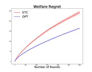
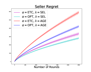
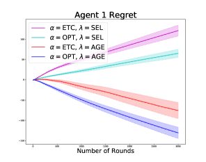
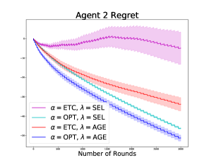
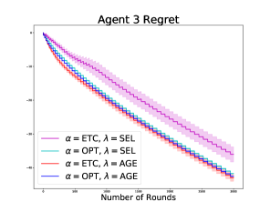
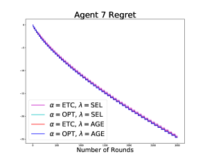
Figure 1: Results for a single-item simulation study. We show the welfare regret, the seller regret, and the regret of four agents for the four difference choices for $(\zeta,\lambda)$ over $3000$ rounds. Lower is better in all plots. Agent $1$ has the highest value, and if the values were known, the item would be assigned to agent $1$. The figures were obtained by averaging over 50 independent runs and the shaded regions represent two standard errors. The jagged shape of the curves is due to the periodic exploration phase in the algorithm. Some of the curves overlap in the last two plots for agents 3 and 10.

8 Proof of Theorem 1

In this section, we present our proof of the lower bound in Section 4. We will first describe notation and definitions that will be used throughout our proofs in Sections 8 and 9.

Notation:

$\mathbb{E},\mathbb{P}$ will denote expectations and probabilities. $\mathbb{E}_{t},\mathbb{P}_{t}$ will denote expectation and probability when conditioned on observations up to time $t-1$; for example, $\mathbb{P}_{t}(\cdot)=\mathbb{P}(\cdot|D_{t})$, where $D_{t}=\{s_{i\ell},Y_{i\ell}\}_{i\leq n,\ell\leq t-1}$.

Recall that $\omega_{\star}=\mathop{\mathrm{argmax}}_{\omega}V(\omega)$ is the socially optimal outcome. Let $s_{i\star}=s_{i}(\omega_{\star})$ be the allocation for agent $i$ at the optimum. Similarly, $V^{\shortminus i}$ and $\omega^{\shortminus i}_{\star}$, defined below, will denote the welfare without agent $i$ and its optimiser respectively.

$$V^{\shortminus i}(\omega)=v_{0}(\omega)+\sum_{j\neq i}v_{i}(\omega_{t}),\hskip 25.29494pt\omega^{\shortminus i}_{\star}=\mathop{\mathrm{argmax}}_{\omega\in\Omega}V^{\shortminus i}(\omega).$$ (9)

We will first state the following fact, which is straightforward to verify, regarding agent and seller utilities in the VCG mechanism.

Fact 7

When the outcome and the prices are chosen according to the VCG mechanism,

$$u_{i\star} =v_{i}(s_{i\star})-p_{i\star}=V(\omega_{\star})-V^{\shortminus i}(\omega^{\shortminus i}_{\star}),$$

$$u_{0\star} =v_{0}(\omega_{\star})+\sum_{i=1}^{n}p_{i\star}=\sum_{i=1}^{n}V^{\shortminus i}(\omega^{\shortminus i}_{\star})-(n-1)V(\omega_{\star}).$$

Our second result expresses the regret terms in (3) in a way that is convenient for analysis. For this, we define quantities $H_{T},W_{T}$ below.

$$H_{T}=\frac{1}{T}\sum_{i=1}^{n}\sum_{t=1}^{T}\left(p_{it}+V^{\shortminus i}(\omega_{t})\right),\hskip 36.135ptW_{T}=H_{T}-\sum_{i=1}^{n}V^{\shortminus i}(\omega^{\shortminus i}_{\star}).$$ (10)

$H_{T}$ is computed using observations from rounds $1$ to $T$, and can be thought of as the algorithm’s estimate of $\sum_{i}V^{\shortminus i}(\omega_{\star})$ at the end of $T$ rounds. The following lemma expresses $R^{\rm a}_{T}$ and $R_{0T}$ in terms of $R^{\rm w}_{T}$ and $W_{T}$.

Lemma 8

Let $R^{\rm a}_{T},R_{0T},R^{\rm w}_{T}$ be as defined in (3). Then,

$$R^{\rm a}_{T}=nR^{\rm w}_{T}+TW_{T},\hskip 72.26999ptR_{0T}=-(n-1)R^{\rm w}_{T}-TW_{T}.$$

Proof  Let $h_{it}=p_{it}+V^{\shortminus i}(\omega_{t})$ so that $H_{T}=\frac{1}{T}\sum_{i=1}^{n}\sum_{t=1}^{T}h_{it}$. For agent $i$, we can use Fact 7 and the fact that $u_{it}=v_{i}(\omega_{t})-p_{it}=V(\omega_{t})-h_{it}$ to obtain,

$$u_{i\star}-u_{it}=(V(\omega_{\star})-V(\omega^{\shortminus i}_{\star}))-(V(\omega_{t})-h_{it})=(V(\omega_{\star})-V(\omega_{t}))+(h_{it}-V(\omega^{\shortminus i}_{\star})).$$

Then, since $R^{\rm a}_{T}=\sum_{i}\sum_{t}(u_{i\star}-u_{it})$, we have

$$R^{\rm a}_{T} =\sum_{t=1}^{T}\sum_{i=1}^{n}\left((V(\omega_{\star})-V(\omega_{t}))+(h_{it}-V(\omega^{\shortminus i}_{\star}))\right)$$

$$=n\sum_{t=1}^{T}(V(\omega_{\star})-V(\omega_{t}))\;+\;T\left(H_{T}-\sum_{i=1}^{n}V^{\shortminus i}(\omega^{\shortminus i}_{\star})\right)\,.$$

This proves the first claim. For the seller, at time $t$, we observe

$$u_{0t}=v_{0}(\omega_{t})+\sum_{i=1}^{n}p_{it}=v_{0}(\omega_{t})+\sum_{i=1}^{n}h_{it}-\sum_{i=1}^{n}V^{\shortminus i}(\omega_{t})=\sum_{i=1}^{n}h_{it}-(n-1)V(\omega_{t}).$$

As before, we can now use Fact 7 to write,

$$R_{0T} =\sum_{t=1}^{T}\left(u_{0\star}-u_{0t}\right)=\sum_{t=1}^{T}\sum_{i=1}^{n}\left(V^{\shortminus i}(\omega^{\shortminus i}_{\star})-h_{it}\right)+(n-1)\sum_{t=1}^{T}(V(\omega_{t})-V(\omega_{\star})).$$

The claim follows by observing that the first term in the RHS is $-TW_{T}$ and that the second term is $-R^{\rm w}_{T}$. $\square$

Our proof of Theorem 1 uses techniques from binary hypothesis testing to establish a lower bound on the VCG regret. For this, we begin by reviewing some facts about the KL divergence ${\rm KL}(\cdot\|\cdot)$. Recall that for two probabilities $P,Q$ with $Q$ absolutely continuous with respect to $P$, the KL divergence is ${\rm KL}(P\|Q)=\mathbb{E}_{P}\big{[}\big{(}\frac{\mathrm{d}P}{\mathrm{d}Q}(X)\big{)}\big{]}$. For distributions $P,P^{\prime},Q,Q^{\prime}$ with ${\rm\bf supp}\,(P)={\rm\bf supp}\,(Q)$ and ${\rm\bf supp}\,(P^{\prime})={\rm\bf supp}\,(Q^{\prime})$, the KL divergence between the product distributions satisfies ${\rm KL}(P\times P^{\prime}\|Q\times Q^{\prime})={\rm KL}(P\|Q)+{\rm KL}(P^{\prime}\|Q^{\prime})$. Additionally, for two univariate Gaussians $\mathcal{N}(\mu_{1},1),\mathcal{N}(\mu_{2},1)$, we know ${\rm KL}(\mathcal{N}(\mu_{1},1)\|\mathcal{N}(\mu_{2},1))=(\mu_{1}-\mu_{2})^{2}/2$. The following result from Tsybakov (2008) will be useful in our proof.

Lemma 9 (Tsybakov (2008), Lemmas 2.1 and 2.6)

Let $P,Q$ be probabilities such that $Q$ is absolutely continuous with respect to $P$. Let $A$ be any event. Then,

$$P(A)+Q(A^{c})\geq\frac{1}{2}\exp\big{(}-{\rm KL}(P\|Q)\big{)}.$$

We are now ready to prove the theorem.

Proof of Theorem 1. Let $n>1$. Since the maximum is larger than an average, for any set of real numbers $\{a_{i}\}_{i}$, we have $\max(\{a_{i}\}_{i})\geq\sum_{i}\alpha_{i}a_{i}$ for any $\{\alpha_{i}\}_{i}$ such that $\alpha_{i}\geq 0$, $\sum_{i}\alpha_{i}=1$. Using Lemma 8 and the fact that $R^{\rm w}_{T}$ is positive, we obtain the following two upper bounds on $\max(nR^{\rm w}_{T},R^{\rm a}_{T},R_{0T})$:

$$\max(nR^{\rm w}_{T},R^{\rm a}_{T},R_{0T}) \geq\frac{4}{5}nR^{\rm w}_{T}+\frac{1}{5}R_{0T}\geq\frac{2}{5}nR^{\rm w}_{T}-\frac{1}{5}TW_{T},$$

$$\max(nR^{\rm w}_{T},R^{\rm a}_{T},R_{0T}) \geq\frac{4}{5}nR^{\rm w}_{T}+\frac{1}{5}TR^{\rm a}_{T}=nR^{\rm w}_{T}+\frac{1}{5}TW_{T}\geq\frac{2}{5}nR^{\rm w}_{T}+\frac{1}{5}TW_{T}.$$

The LHS should be larger than both of the above lower bounds. Since $\max(a+b,a+c)=a+\max(b,c)$, we have,

$$R^{\rm{\tiny VCG}}_{T}=\max(nR^{\rm w}_{T},R^{\rm a}_{T},R_{0T}) \geq\frac{2}{5}nR^{\rm w}_{T}+\frac{1}{5}T|W_{T}|\;\,\stackrel{{\scriptstyle\Delta}}{{=}}Q_{T}.$$

We will obtain a lower bound on $\inf_{\mathcal{A}}\sup_{\Theta}\mathbb{E}Q_{T}$ which translates to a lower bound on the desired quantity. Our strategy for doing so is to consider two problems in $\Theta$ and show that any algorithm will not be able to distinguish between them. Both problems will have the same set of outcomes $\Omega=\{0,1,\dots,\dots,|\Omega|-1\}$ with $\Omega={\mathcal{S}}$ and $|\Omega|\geq n+1$. In the first problem, henceforth called $\theta_{0}$, the optimal outcome is $0$ with $v_{i}(0)=1/2$ for all agents $i$. For outcome $j\in\{1,\dots,n\}$, $v_{j}(j)=0$ and $v_{i}(j)=1/2$ for every other agent $i\neq j$. For $j>n$, $v_{i}(j)<1/4$ for all $i$. When an outcome $\omega$ is chosen, agent $i$ realises a value drawn from $\mathcal{N}(v_{i}(\omega),1)$. Finally, the seller has $0$ value for all outcomes, $v_{0}(j)=0$ for all $j\in\Omega$. The following statements are true about problem $\theta_{0}$:

$$V(\omega_{\star})=V(0)=\frac{n}{2},\hskip 28.90755ptV^{\shortminus i}(\omega^{\shortminus i}_{\star})=V(i)=\frac{n}{2}-\frac{1}{2},\hskip 28.90755pt\sum_{i=1}^{n}V^{\shortminus i}(\omega^{\shortminus i}_{\star})=\frac{n^{2}}{2}-\frac{n}{2}.$$

The second problem, henceforth called $\theta_{1}$, is the same as $\theta_{0}$ but differs in outcomes $j\in\{1,\dots,n\}$, as shown below. Here, the value of $\delta\in(0,1/(2(n-1)))$ will be specified shortly. We have:

$$v_{i}(j)=\begin{cases}0\hskip 28.90755pt&\quad\text{if $i=j$},\\ \frac{1}{2}+\delta\quad&\quad\text{if $i\neq j$}.\end{cases}$$

The following statements are true about problem $\theta_{1}$:

$$V(\omega_{\star})=V(0)=\frac{n}{2},\hskip 28.90755ptV^{\shortminus i}(\omega^{\shortminus i}_{\star})=V(i)=\frac{n}{2}-\frac{1}{2}+(n-1)\delta,$$

$$\sum_{i=1}^{n}V^{\shortminus i}(\omega^{\shortminus i}_{\star})=\frac{n^{2}}{2}-\frac{n}{2}+n(n-1)\delta.$$

In the above problems, if $\delta$ is set to be too large, then it becomes easier to distinguish between the values of different outcomes using stochastic observations thus making the problem easy. If $\delta$ is set to be too small, then the regret terms become small since all outcomes have similar values. The largest lower bound is obtained by careful choice of $\delta$ (dependent on both $n$ and $T$) so as to balance between these two cases.

We will make the dependence of $Q_{T}$ on the problem explicit and write $Q_{T}(\theta_{0}),Q_{T}(\theta_{1})$ respectively. Consider any algorithm in $\mathcal{A}$. Expectations and probabilities when we execute this algorithm problem in $\theta_{0}$ will be denoted $\mathbb{E}_{\theta_{0}},\mathbb{P}_{\theta_{0}}$, and in problem $\theta_{1}$, they will be denoted $\mathbb{E}_{\theta_{1}},\mathbb{P}_{\theta_{1}}$. Let $N_{t}(\omega)=\sum_{i=1}^{t-1}\mathbbm{1}(\omega_{t}=\omega)$ denote the number of times outcome $\omega\in\Omega$ was chosen in the first $t-1$ time steps. With this notation, we can upper bound the welfare regret in problem $\theta\in\{\theta_{0},\theta_{1}\}$ as,

$$\mathbb{E}_{\theta}[R^{\rm w}_{T}]=\sum_{j\geq 1}(V(0)-V(j))\mathbb{E}_{\theta}[N_{t}(j)]\geq\sum_{j=1}^{n}(V(0)-V(j))\mathbb{E}_{\theta}[N_{t}(j)].$$

Using the observation that the gap between the optimal and any other outcome in problem $\theta_{0}$ is at least $1/2$, and that when $H_{T}>n^{2}/2-n/2+n(n-1)\delta/2$, $|W_{T}|$ is at least $n(n-1)\delta/2$, we obtain the following lower bound on $\mathbb{E}_{\theta_{0}}[Q_{T}(\theta_{0})]$:

$$\mathbb{E}_{\theta_{0}}[Q_{T}(\theta_{0})] \geq\;\frac{2n}{5}\sum_{k=1}^{n}\frac{1}{2}\mathbb{E}_{\theta_{0}}\left[N_{t+1}(k)\right]\;+\;\frac{T}{5}\frac{n(n-1)\delta}{2}\,\mathbb{P}_{\theta_{0}}\bigg{(}\underbrace{\vphantom{\Bigg{(}}H_{T}>\frac{n^{2}}{2}-\frac{n}{2}+\frac{1}{2}n(n-1)\delta}_{\text{event }A}\bigg{)},$$

$$\geq\;\frac{n}{10}\Bigg{(}\;\sum_{k=1}^{n}2\mathbb{E}_{\theta_{0}}\left[N_{t+1}(k)\right]\;+\;Tn(n-1)\delta\;\mathbb{P}_{\theta_{0}}(A)\;\Bigg{)}.$$ (11)

By a similar argument regarding $H_{T}$ under the event $A^{c}$ in problem $\theta_{1}$, we obtain the following. Here, we have dropped the $\mathbb{E}_{\theta_{1}}\left[N_{t+1}(k)\right]$ terms which are positive.

$$\mathbb{E}_{\theta_{1}}[Q_{T}(\theta_{1})] \geq\;\frac{n}{10}Tn(n-1)\delta\;\mathbb{P}_{\theta_{1}}(A^{c}).$$

To combine these results we will apply Lemma 9 on $\mathbb{P}_{\theta_{0}}(A)+\mathbb{P}_{\theta_{0}}^{\prime}(A^{c})$ in a manner similar to Bubeck et al. (2013). Letting $\theta^{T}_{0},\theta^{T}_{1}$ denote the probability laws of the observed rewards up to round $T$ in problems $\theta_{0},\theta_{1}$ respectively, we obtain

$$\mathbb{P}_{\theta_{0}}(A)+\mathbb{P}_{\theta_{0}}^{\prime}(A^{c})\geq\frac{1}{2}\exp\left(-{\rm KL}(\theta^{T}_{0}\|\theta^{T}_{1})\right)=\frac{1}{2}\exp\left(-\frac{(n-1)\delta^{2}}{2}\sum_{j=1}^{n}\mathbb{E}_{\theta_{0}}[N_{T+1}(j)]\right).$$

For the first step we have used the fact that $A$ is measurable with respect to the $\sigma$-field generated by observations up to round $T$. For the second step, observe that the outcomes $0,n+1,n+2,|\Omega|-1$ have the same distributions under both $\theta_{0}$ and $\theta_{1}$. For any outcome $i\in\{1,\dots,n\}$, the distribution of agent $i$ is also the same in both problems. For all other agents $j\neq i$, the KL divergence between the corresponding distributions in the two problems is $\delta^{2}/2$. By combining the three previous bounds, we obtain an upper bound on $\mathbb{E}_{\theta_{0}}[Q_{T}(\theta_{0})]+\mathbb{E}_{\theta_{1}}[Q_{T}(\theta_{1})]$:

$$\frac{10}{n}\Big{(}\mathbb{E}_{\theta_{0}} [Q_{T}(\theta_{0})]+\mathbb{E}_{\theta_{1}}[Q_{T}(\theta_{1})]\Big{)}$$

$$\geq\;\sum_{k=1}^{n}2\mathbb{E}_{\theta_{0}}\left[N_{t+1}(k)\right]\;+\;T(n-1)\delta\;\Big{(}\mathbb{P}_{\theta_{0}}(A)+\mathbb{P}_{\theta_{0}}^{\prime}(A^{c})\Big{)},$$

$$\geq\;2\sum_{k=1}^{n}\mathbb{E}_{\theta_{0}}\left[N_{t+1}(k)\right]\;+\;\frac{1}{2}T(n-1)\delta\;\exp\left(-\frac{(n-1)\delta^{2}}{2}\sum_{k=1}^{n}\mathbb{E}_{\theta_{0}}[N_{t+1}(k)]\right)$$

$$\geq\;\min_{x}\left\{2x\;+\;\frac{1}{2}T(n-1)\delta\;\exp\left(-\frac{(n-1)\delta^{2}}{2}x\right)\right\}$$

$$\geq\frac{4}{(n-1)\delta^{2}}\log\left(\frac{T(n-1)^{2}\delta^{3}}{8}\right).$$

Finally, we choose $\delta=\left(\frac{16}{T(n-1)^{2}}\right)^{1/3}$ so that the $\log$ term above can be upper bounded by a constant. This results in the following bound:

$$\frac{1}{2}\Big{(}\mathbb{E}_{\theta_{0}}[Q_{T}(\theta_{0})]+\mathbb{E}_{\theta_{1}}[Q_{T}(\theta_{1})]\Big{)}\geq\;\frac{\log(2)}{5\cdot 16^{\nicefrac{{2}}{{3}}}}\cdot T^{\nicefrac{{2}}{{3}}}(n-1)^{\nicefrac{{4}}{{3}}},$$

where $\delta<\frac{1}{2(n-1)}$ is satisfied if $T>128n$. The claim follows by observing $\;\sup_{\theta\in\Theta}\mathbb{E}[Q_{T}(\theta)]\geq\max\left(\mathbb{E}_{\theta_{0}}[Q_{T}(\theta_{0})],\mathbb{E}_{\theta_{1}}[Q_{T}(\theta_{1})]\right)\geq\frac{1}{2}\mathbb{E}_{\theta_{0}}[Q_{T}(\theta_{0})]+\frac{1}{2}\mathbb{E}_{\theta_{1}}[Q_{T}(\theta_{1})]$. $\blacksquare$

9 Proofs of Results in Section 6

In this section, we analyse Algorithm 1. Section 9.1 controls the probability that the confidence intervals given in (4) capture the true values. The proofs of Theorems 2, 3, and 4 are given in Sections 9.2, 9.3, and 9.6 respectively. Sections 9.4 and 9.5 prove Propositions 5 and 6 respectively. The bounds on $R_{0T}$ and $R^{\rm w}_{T}$ will be useful in bounding $R^{\rm{\tiny VCG}}_{T}$. In Section 9.7, we state some technical results that are used in our proofs. We begin with some notation and definitions.

Notation & Definitions:

Recall that Algorithm 1 proceeds in a sequence of brackets. In our proofs, $q_{t}$ will denote the bracket index round $t$ belongs to and $T_{q}$ will be the number of rounds completed by $q$ brackets. Then,

$$T_{q_{t}-1}<t\leq T_{q_{t}}.$$ (12)

$\mathcal{E}_{it}$, defined below, will denote the event that agent $i$’s values are trapped by the lower and upper confidence bounds at round $t$ when she participates truthfully. $\mathcal{E}_{t}$ denotes the same for all agents. Here $\widehat{v}_{it},{\mathchoice{{\ooalign{\hbox{\raise 6.25pt\hbox{\scalebox{1.0}[-1.0]{\lower 6.25pt\hbox{$\displaystyle\widehat{\vrule width=0.0pt,height=4.30554pt\vrule height=0.0pt,width=5.20601pt}$}}}}\cr\hbox{$\displaystyle v$}}}}{{\ooalign{\hbox{\raise 6.25pt\hbox{\scalebox{1.0}[-1.0]{\lower 6.25pt\hbox{$\textstyle\widehat{\vrule width=0.0pt,height=4.30554pt\vrule height=0.0pt,width=5.20601pt}$}}}}\cr\hbox{$\textstyle v$}}}}{{\ooalign{\hbox{\raise 5.81944pt\hbox{\scalebox{1.0}[-1.0]{\lower 5.81944pt\hbox{$\scriptstyle\widehat{\vrule width=0.0pt,height=3.01389pt\vrule height=0.0pt,width=3.64421pt}$}}}}\cr\hbox{$\scriptstyle v$}}}}{{\ooalign{\hbox{\raise 5.53241pt\hbox{\scalebox{1.0}[-1.0]{\lower 5.53241pt\hbox{$\scriptscriptstyle\widehat{\vrule width=0.0pt,height=2.15277pt\vrule height=0.0pt,width=2.603pt}$}}}}\cr\hbox{$\scriptscriptstyle v$}}}}}_{it}$ are as defined in (4). We have:

$$\mathcal{E}_{it}=\Big{(}\forall\,s\in{\mathcal{S}},\;\,v_{i}(s)\in[{\mathchoice{{\ooalign{\hbox{\raise 6.25pt\hbox{\scalebox{1.0}[-1.0]{\lower 6.25pt\hbox{$\displaystyle\widehat{\vrule width=0.0pt,height=4.30554pt\vrule height=0.0pt,width=5.20601pt}$}}}}\cr\hbox{$\displaystyle v$}}}}{{\ooalign{\hbox{\raise 6.25pt\hbox{\scalebox{1.0}[-1.0]{\lower 6.25pt\hbox{$\textstyle\widehat{\vrule width=0.0pt,height=4.30554pt\vrule height=0.0pt,width=5.20601pt}$}}}}\cr\hbox{$\textstyle v$}}}}{{\ooalign{\hbox{\raise 5.81944pt\hbox{\scalebox{1.0}[-1.0]{\lower 5.81944pt\hbox{$\scriptstyle\widehat{\vrule width=0.0pt,height=3.01389pt\vrule height=0.0pt,width=3.64421pt}$}}}}\cr\hbox{$\scriptstyle v$}}}}{{\ooalign{\hbox{\raise 5.53241pt\hbox{\scalebox{1.0}[-1.0]{\lower 5.53241pt\hbox{$\scriptscriptstyle\widehat{\vrule width=0.0pt,height=2.15277pt\vrule height=0.0pt,width=2.603pt}$}}}}\cr\hbox{$\scriptscriptstyle v$}}}}}_{it}(s),\widehat{v}_{it}(s)]\Big{)},\hskip 43.36243pt\mathcal{E}_{t}=\bigcap_{i=1}^{n}\mathcal{E}_{it}.$$

For the outcome $\omega_{t}$ at time $t$, let $s_{it}=s_{i}(\omega_{t})$ be the allocation for agent $i$. Hence, for instance, we can write $V(\omega_{t})=v_{0}(\omega_{t})+\sum_{i=1}^{n}v_{i}(\omega_{t})=v_{0}(\omega_{t})+\sum_{i=1}^{n}v_{i}(s_{it})$. We will similarly use the following definitions for the upper and lower bound on the welfare at time $t$, the functions $F^{\shortminus i}_{t},G^{\shortminus i}_{t}$ used in the pricing calclulation, and their optimisers. Some of these terms have been defined before.

$$\widehat{V}_{t}(\omega)=v_{0}(\omega)+\sum_{i=1}^{n}\widehat{v}_{it}(\omega_{t}),\hskip 10.84006pt\omega_{t}=\mathop{\mathrm{argmax}}_{\omega\in\Omega}\widehat{V}_{t}(\omega),\hskip 18.06749pt{\mathchoice{{\ooalign{\hbox{\raise 7.09259pt\hbox{\scalebox{1.0}[-1.0]{\lower 7.09259pt\hbox{$\displaystyle\widehat{\vrule width=0.0pt,height=6.83331pt\vrule height=0.0pt,width=8.05556pt}$}}}}\cr\hbox{$\displaystyle V$}}}}{{\ooalign{\hbox{\raise 7.09259pt\hbox{\scalebox{1.0}[-1.0]{\lower 7.09259pt\hbox{$\textstyle\widehat{\vrule width=0.0pt,height=6.83331pt\vrule height=0.0pt,width=8.05556pt}$}}}}\cr\hbox{$\textstyle V$}}}}{{\ooalign{\hbox{\raise 6.40926pt\hbox{\scalebox{1.0}[-1.0]{\lower 6.40926pt\hbox{$\scriptstyle\widehat{\vrule width=0.0pt,height=4.78333pt\vrule height=0.0pt,width=5.63889pt}$}}}}\cr\hbox{$\scriptstyle V$}}}}{{\ooalign{\hbox{\raise 5.9537pt\hbox{\scalebox{1.0}[-1.0]{\lower 5.9537pt\hbox{$\scriptscriptstyle\widehat{\vrule width=0.0pt,height=3.41666pt\vrule height=0.0pt,width=4.02777pt}$}}}}\cr\hbox{$\scriptscriptstyle V$}}}}}_{t}(\omega)=v_{0}(\omega)+\sum_{i=1}^{n}{\mathchoice{{\ooalign{\hbox{\raise 6.25pt\hbox{\scalebox{1.0}[-1.0]{\lower 6.25pt\hbox{$\displaystyle\widehat{\vrule width=0.0pt,height=4.30554pt\vrule height=0.0pt,width=5.20601pt}$}}}}\cr\hbox{$\displaystyle v$}}}}{{\ooalign{\hbox{\raise 6.25pt\hbox{\scalebox{1.0}[-1.0]{\lower 6.25pt\hbox{$\textstyle\widehat{\vrule width=0.0pt,height=4.30554pt\vrule height=0.0pt,width=5.20601pt}$}}}}\cr\hbox{$\textstyle v$}}}}{{\ooalign{\hbox{\raise 5.81944pt\hbox{\scalebox{1.0}[-1.0]{\lower 5.81944pt\hbox{$\scriptstyle\widehat{\vrule width=0.0pt,height=3.01389pt\vrule height=0.0pt,width=3.64421pt}$}}}}\cr\hbox{$\scriptstyle v$}}}}{{\ooalign{\hbox{\raise 5.53241pt\hbox{\scalebox{1.0}[-1.0]{\lower 5.53241pt\hbox{$\scriptscriptstyle\widehat{\vrule width=0.0pt,height=2.15277pt\vrule height=0.0pt,width=2.603pt}$}}}}\cr\hbox{$\scriptscriptstyle v$}}}}}_{it}(\omega_{t}),$$

$$F^{\shortminus i}_{t}(\omega)=v_{0}(\omega)+\sum_{j\neq i}f_{it}(\omega_{t}),\hskip 10.84006pt\omega^{\shortminus i}_{t}=\mathop{\mathrm{argmax}}_{\omega\in\Omega}F^{\shortminus i}_{t}(\omega),$$ (14)

$$G^{\shortminus i}_{t}(\omega)=v_{0}(\omega)+\sum_{j\neq i}g_{it}(\omega_{t}),\hskip 18.06749ptG_{t}(\omega)=v_{0}(\omega)+\sum_{i=1}^{n}g_{it}(\omega_{t}).$$

Next, we define some quantities related to the mean and confidence intervals defined in (4). For brevity, we will denote the unclipped empirical mean in (4) by $\overline{v}^{\prime}_{it}(s)$. Next, we define $\beta_{t},\sigma_{it}$ as shown below. With this, we can rewrite the upper and lower confidence bounds in (4) as follows:

$$\beta_{t}=\sqrt{5\log(t-qK+1)+2\log(|{\mathcal{S}}|)},\hskip 25.29494pt\sigma_{it}(s)=\begin{cases}\,0\hskip 7.22743pt&\text{if $i$ plays by bids}\\ \,\frac{\sigma}{\sqrt{N_{it}(s)}}\hskip 7.22743pt&\text{otherwise}\end{cases},$$ (15)

$$\widehat{v}_{it}(s)=\overline{v}_{it}(s)+\beta_{t}\sigma_{it}(s),\hskip 79.49744pt{\mathchoice{{\ooalign{\hbox{\raise 6.25pt\hbox{\scalebox{1.0}[-1.0]{\lower 6.25pt\hbox{$\displaystyle\widehat{\vrule width=0.0pt,height=4.30554pt\vrule height=0.0pt,width=5.20601pt}$}}}}\cr\hbox{$\displaystyle v$}}}}{{\ooalign{\hbox{\raise 6.25pt\hbox{\scalebox{1.0}[-1.0]{\lower 6.25pt\hbox{$\textstyle\widehat{\vrule width=0.0pt,height=4.30554pt\vrule height=0.0pt,width=5.20601pt}$}}}}\cr\hbox{$\textstyle v$}}}}{{\ooalign{\hbox{\raise 5.81944pt\hbox{\scalebox{1.0}[-1.0]{\lower 5.81944pt\hbox{$\scriptstyle\widehat{\vrule width=0.0pt,height=3.01389pt\vrule height=0.0pt,width=3.64421pt}$}}}}\cr\hbox{$\scriptstyle v$}}}}{{\ooalign{\hbox{\raise 5.53241pt\hbox{\scalebox{1.0}[-1.0]{\lower 5.53241pt\hbox{$\scriptscriptstyle\widehat{\vrule width=0.0pt,height=2.15277pt\vrule height=0.0pt,width=2.603pt}$}}}}\cr\hbox{$\scriptscriptstyle v$}}}}}_{it}(s)=\overline{v}_{it}(s)-\beta_{t}\sigma_{it}(s).$$

9.1 Bounding $\mathbb{P}_{t}(\mathcal{E}^{c}_{t})$

In this section, we control the probability that the upper and lower confidence bounds do not trap the true values $\{v_{i}(s)\}_{i,s}$. Recall that sub-Gaussian random variables satisfy the following concentration property. Let $\{X_{i}\}_{i=1}^{n}$ be $n$ i.i.d samples from a $\sigma$ sub-Gaussian distribution and $\overline{X}=\frac{1}{n}\sum_{i}X_{i}$ be its sample mean. Then,

$$\mathbb{P}(\overline{X}>\epsilon)\leq e^{\frac{-n\epsilon^{2}}{2\sigma^{2}}},\hskip 32.52127pt\mathbb{P}(\overline{X}<\epsilon)\leq e^{\frac{-n\epsilon^{2}}{2\sigma^{2}}}.$$

Lemma 10

Assume that agent $i$ participates truthfully and let $\mathcal{E}_{it}$ be as defined in (9). When $\zeta={\text{\scriptsize{ETC}}}$, for $t\notin{\rm\bf E}$ in bracket $q$, $\mathbb{P}_{t}(\mathcal{E}^{c}_{it})\leq 2(t-qK)^{-\nicefrac{{5}}{{2}}}$. Moreover, for all $T$, $\sum_{t=1,t\notin{\rm\bf E}}^{T}\mathbb{P}_{t}(\mathcal{E}^{c}_{t})\leq 4$. When $\zeta={\text{\scriptsize{OPT}}}$, for $t\notin{\rm\bf E}$ in bracket $q$, $\mathbb{P}_{t}(\mathcal{E}^{c}_{it})\leq 2(t-qK)^{-\nicefrac{{3}}{{2}}}$. Moreover, for all $T$, $\sum_{t=1,t\notin{\rm\bf E}}^{T}\mathbb{P}_{t}(\mathcal{E}^{c}_{t})\leq 6$.

Proof  If the agent participates by bids truthfully, then $\widehat{v}_{it}={\mathchoice{{\ooalign{\hbox{\raise 6.25pt\hbox{\scalebox{1.0}[-1.0]{\lower 6.25pt\hbox{$\displaystyle\widehat{\vrule width=0.0pt,height=4.30554pt\vrule height=0.0pt,width=5.20601pt}$}}}}\cr\hbox{$\displaystyle v$}}}}{{\ooalign{\hbox{\raise 6.25pt\hbox{\scalebox{1.0}[-1.0]{\lower 6.25pt\hbox{$\textstyle\widehat{\vrule width=0.0pt,height=4.30554pt\vrule height=0.0pt,width=5.20601pt}$}}}}\cr\hbox{$\textstyle v$}}}}{{\ooalign{\hbox{\raise 5.81944pt\hbox{\scalebox{1.0}[-1.0]{\lower 5.81944pt\hbox{$\scriptstyle\widehat{\vrule width=0.0pt,height=3.01389pt\vrule height=0.0pt,width=3.64421pt}$}}}}\cr\hbox{$\scriptstyle v$}}}}{{\ooalign{\hbox{\raise 5.53241pt\hbox{\scalebox{1.0}[-1.0]{\lower 5.53241pt\hbox{$\scriptscriptstyle\widehat{\vrule width=0.0pt,height=2.15277pt\vrule height=0.0pt,width=2.603pt}$}}}}\cr\hbox{$\scriptscriptstyle v$}}}}}_{it}=v_{i}$ and the claim is trivially true. For agents participating by rewards, we will first prove this for $\zeta={\text{\scriptsize{OPT}}}$. Consider the event $\{v_{i}(s)>\widehat{v}_{it}(s)\}$ and recall the definitions in (4). Let $\overline{v}^{\prime}_{it}(s)$ be the unclipped empirical mean in (4). Let $\overline{\vphantom{\rule{1.0pt}{5.5pt}}\smash{\overline{v}}}_{it}(s)=\max(0,\overline{v}^{\prime}_{it}(s))$ and $\widehat{\vphantom{\rule{1.0pt}{5.5pt}}\smash{\widehat{v}}}_{it}(s)=\overline{\vphantom{\rule{1.0pt}{5.5pt}}\smash{\overline{v}}}_{it}(s)+\beta_{t}\sigma_{it}(s)$. Since $\overline{v}_{it}(s)=\min(1,\overline{\vphantom{\rule{1.0pt}{5.5pt}}\smash{\overline{v}}}_{it}(s))$, we have $\widehat{\vphantom{\rule{1.0pt}{5.5pt}}\smash{\widehat{v}}}_{it}(s)\geq\widehat{v}_{it}(s)$. However, the following calculations show that $\mathbb{P}\left(v_{i}(s)>\widehat{v}_{it}(s)\right)=\mathbb{P}(v_{i}(s)>\widehat{\vphantom{\rule{1.0pt}{5.5pt}}\smash{\widehat{v}}}_{it}(s))$.

$$\mathbb{P}_{t}\left(v_{i}(s)>\widehat{v}_{it}(s)\right)$$

$$=\mathbb{P}_{t}\left(v_{i}(s)>\widehat{v}_{it}(s)|\overline{v}^{\prime}_{it}(s)\geq 1\right)\mathbb{P}_{t}(\overline{v}^{\prime}_{it}(s)\geq 1)+\mathbb{P}_{t}\left(v_{i}(s)>\widehat{v}_{it}(s)|\overline{v}^{\prime}_{it}(s)<1\right)\mathbb{P}_{t}(\overline{v}^{\prime}_{it}(s)<1)$$

$$=\mathbb{P}_{t}\left(v_{i}(s)>\widehat{\vphantom{\rule{1.0pt}{5.5pt}}\smash{\widehat{v}}}_{it}(s)|\overline{\vphantom{\rule{1.0pt}{5.5pt}}\smash{\overline{v}}}_{it}(s)\geq 1\right)\mathbb{P}_{t}(\overline{\vphantom{\rule{1.0pt}{5.5pt}}\smash{\overline{v}}}_{it}(s)\geq 1)+\mathbb{P}_{t}\left(v_{i}(s)>\widehat{\vphantom{\rule{1.0pt}{5.5pt}}\smash{\widehat{v}}}_{it}(s)|\overline{\vphantom{\rule{1.0pt}{5.5pt}}\smash{\overline{v}}}_{it}(s)<1\right)\mathbb{P}_{t}(\overline{\vphantom{\rule{1.0pt}{5.5pt}}\smash{\overline{v}}}_{it}(s)<1)$$

$$=\mathbb{P}_{t}\left(v_{i}(s)>\widehat{\vphantom{\rule{1.0pt}{5.5pt}}\smash{\widehat{v}}}_{it}(s)\right).$$

Here, the second step uses two arguments. First, when $\overline{v}^{\prime}_{it}(s)<1$, then $\widehat{v}_{it}(s)=\widehat{\vphantom{\rule{1.0pt}{5.5pt}}\smash{\widehat{v}}}_{it}(s)$. Second, when $\overline{v}^{\prime}_{it}(s)\geq 1$, then $\mathbb{P}_{t}(v_{i}(s)>\widehat{v}_{it}(s))=\mathbb{P}_{t}(v_{i}(s)>\widehat{\vphantom{\rule{1.0pt}{5.5pt}}\smash{\widehat{v}}}_{it}(s))=1$ since $v_{i}(s)\leq 1<\widehat{v}_{it}(s)\leq\widehat{\vphantom{\rule{1.0pt}{5.5pt}}\smash{\widehat{v}}}_{it}(s)$. We can now bound,

$$\mathbb{P}_{t}(v_{i}(s)>\widehat{v}_{it}(s)) =\mathbb{P}_{t}\big{(}v_{i}(s)>\max(0,\overline{v}^{\prime}_{it}(s))+\beta_{t}\sigma_{it}(s)\big{)}$$

$$\leq\mathbb{P}_{t}\bigg{(}v_{i}(s)\,>\,\frac{1}{N_{it}(s)}\sum_{\ell=1}^{t-1}X_{i\ell}\mathbbm{1}(s_{it}=s)+\beta_{t}\frac{\sigma}{\sqrt{N_{it}(s)}}\bigg{)}$$

$$\leq\mathbb{P}_{t}\bigg{(}\exists\tau\in\{q,\dots,t-(K-1)q\},\;v_{i}(s)\,>\,\frac{1}{\tau}\sum_{\ell=1}^{\tau}X^{\prime}_{i\ell}+\beta_{t}\frac{\sigma}{\sqrt{\tau}}\bigg{)}$$

$$\leq\sum_{\tau=q}^{t-qK+q}\mathbb{P}_{t}\bigg{(}v_{i}(s)\,>\,\frac{1}{\tau}\sum_{\ell=1}^{\tau}X^{\prime}_{i\ell}+\beta_{t}\frac{\sigma}{\sqrt{\tau}}\bigg{)}\;\leq\;(t-qK+1)e^{-\beta_{t}^{2}/2}$$

$$\leq\;\frac{1}{|{\mathcal{S}}|(t-qK+1)^{\nicefrac{{3}}{{2}}}}$$

In the second step, if $\overline{v}^{\prime}_{it}(s)$ was clipped below at $0$, then we can replace it with a smaller quantity. In the third step, we have used the fact that $N_{it}(s)$ would take a value in $\{q,\dots,t-(K-1)q\}$ since there have been $qK$ exploration rounds thus far, during which we have collected rewards from agent $i$ for allocation $s$ exactly $q$ times. $\{X^{\prime}_{i\ell}\}_{\ell=1}^{\tau}$ denotes the rewards $X_{i\ell}$ collected when $N_{it}(s)=\tau$. The fourth step uses a union bound and the fourth step applies the sub-Gaussian condition. A similar bound can be shown for the event $\{v_{i}(s)<{\mathchoice{{\ooalign{\hbox{\raise 6.25pt\hbox{\scalebox{1.0}[-1.0]{\lower 6.25pt\hbox{$\displaystyle\widehat{\vrule width=0.0pt,height=4.30554pt\vrule height=0.0pt,width=5.20601pt}$}}}}\cr\hbox{$\displaystyle v$}}}}{{\ooalign{\hbox{\raise 6.25pt\hbox{\scalebox{1.0}[-1.0]{\lower 6.25pt\hbox{$\textstyle\widehat{\vrule width=0.0pt,height=4.30554pt\vrule height=0.0pt,width=5.20601pt}$}}}}\cr\hbox{$\textstyle v$}}}}{{\ooalign{\hbox{\raise 5.81944pt\hbox{\scalebox{1.0}[-1.0]{\lower 5.81944pt\hbox{$\scriptstyle\widehat{\vrule width=0.0pt,height=3.01389pt\vrule height=0.0pt,width=3.64421pt}$}}}}\cr\hbox{$\scriptstyle v$}}}}{{\ooalign{\hbox{\raise 5.53241pt\hbox{\scalebox{1.0}[-1.0]{\lower 5.53241pt\hbox{$\scriptscriptstyle\widehat{\vrule width=0.0pt,height=2.15277pt\vrule height=0.0pt,width=2.603pt}$}}}}\cr\hbox{$\scriptscriptstyle v$}}}}}_{it}(s)\}$. The first claim follows by applying a union bound over these two events and over all $s\in{\mathcal{S}}$. The second claim follows from the observation $\sum_{t=1}^{\infty}t^{-3/2}\leq 1+\int_{1}^{\infty}t^{-3/2}\leq 3$.

Now consider $\zeta={\text{\scriptsize{ETC}}}$. The calculations above can be repeated, except $N_{it}(s)=q_{t}$ (12) deterministically for all $i,t$. (When $\zeta={\text{\scriptsize{OPT}}}$, $N_{it}(s)$ is random and depends on the reward realised.) Therefore, we will not need the sum over $\tau\in\{q,\dots,t-(K-1)q\}$, resulting in the bound $e^{-\beta_{t}^{2}/2}\leq\frac{1}{|{\mathcal{S}}|(t-qK)^{\nicefrac{{5}}{{2}}}}$. The second claim follows from $\sum_{t}t^{-5/2}\leq 2$. $\square$

Lemma 11

Assume that all agents participate truthfully and let $\mathcal{E}_{t}$ be as defined in (9). When $\zeta={\text{\scriptsize{ETC}}}$, for $t\notin{\rm\bf E}$ in bracket $q$, $\mathbb{P}_{t}(\mathcal{E}^{c}_{t})\leq 2n(t-qK)^{-\nicefrac{{5}}{{2}}}$. Moreover, for all $T$, $\sum_{t=1,t\notin{\rm\bf E}}^{T}\mathbb{P}_{t}(\mathcal{E}^{c}_{t})\leq 4n$. When $\zeta={\text{\scriptsize{OPT}}}$, for $t\notin{\rm\bf E}$ in bracket $q$, $\mathbb{P}_{t}(\mathcal{E}^{c}_{t})\leq 2n(t-qK)^{-\nicefrac{{3}}{{2}}}$. Moreover, for all $T$, $\sum_{t=1,t\notin{\rm\bf E}}^{T}\mathbb{P}_{t}(\mathcal{E}^{c}_{t})\leq 6n$.

Proof  This follows by an application of the union bound over the agents $i\in\{1,\dots,n\}$ on the results of Lemma 10. $\square$

9.2 Proof of Theorem 2

We will first prove Theorem 2. We begin with the following Lemma. To state it, consider any strategy $\pi$ that agent $i$ may follow when reporting her rewards. Let $u_{it}$ be the utility of the agent on round $t$ when she reports truthfully on rounds $1$ to $t-1$ (recall that the allocation the agent receives on round $t$ depends on the rewards $\{Y_{i\ell}\}_{\ell=1}^{t-2}$ she reported on rounds in the first $t-1$ rounds), let $u^{\pi}_{it}$ be the utility of the agent when she follows strategy $\pi$ from rounds 1 through $t-1$, and let $u^{t-1}_{it}$ be the utility of agent on round $t$ when she follows $\pi$ on rounds 1 thorough $t-2$ and then switches to truth-telling at the end of round $t-1$. If participating by bids, this means it will change the bid function, and if participating by rewards, it means it will replace the reported rewards $Y_{i\ell}$ for rounds $1,\dots,t-2$ with the true rewards $X_{i\ell}$ and then report truthfully at round $t-1$. Agent $i$’s allocation at round $t$ when the agent replaces her rewards this way will be different to the allocation chosen when simply reporting truthfully since her past untruthful behaviour will have affected the outcomes chosen by the mechanism in the previous rounds (this is particularly the case when $\zeta={\text{\scriptsize{OPT}}}$). We should also emphasise that this behaviour of replacing the rewards is only for the purposes of our proof below. We have the following result.

Lemma 12

Let $u_{it},u^{\pi}_{it},u^{t-1}_{it}$ be as defined above. Then,

$$U^{\pi}_{iT}-U_{iT}=\sum_{t=1}^{T}u^{\pi}_{it}-u^{t-1}_{it}+\sum_{t=2}^{T}u^{t-1}_{it}-u_{it}.$$ (16)

Proof  The claim follows by adding and subtracting $\sum_{t=1}^{T}u^{t-1}_{it}$, rearranging the terms, and noting that $u^{0}_{i1}=u_{i1}$. $\square$

When applying the above Lemma, we will denote the strategy which follows $\pi$ up to round $t-2$ and switches to truth-telling at the end of round $t-1$ as $\pi^{t-1}$. We will denote the outcomes at round $t$ when following $\pi$, $\pi^{t-1}$ and truth-telling by $\omega^{\pi}_{t},\omega^{t-1}_{t}$ and $\omega_{t}$ respectively, and the allocations for agent $i$ by $s^{\pi}_{it},s^{r}_{it},s_{it}$ for respectively; therefore, $s^{\pi}_{it}=s_{i}(\omega^{\pi}_{t})$, $s^{r}_{it}=s_{i}(\omega^{t-1}_{t}$, and $s_{it}=s_{i}(\omega_{t})$.

9.2.1 Proof of Theorem 2.1

We begin with Lemma 12. First, consider the second summation in its RHS, where we claim that each term inside the summation is $0$. To see this, note that $\pi^{t-1}$ is also participating truthfully at round $t$. It has replaced its reported rewards with its true realised rewards in the previous rounds. The mechanism only uses rewards reported in the exploration rounds to decide outcomes on the exploitation rounds, and the outcomes in the exploration rounds are chosen independent of the bids/rewards reported by the agent. As the outcome and prices in round $t$ will be the same for both policies, we have $u^{t-1}_{it}=u_{it}$. (As we will see shortly in Section 9.2.2, this will not be the case when $\zeta={\text{\scriptsize{OPT}}}$, and the second sum will be non-zero.)

Now turn to the first summation in the RHS of 12. In the remainder of the proof, $g_{it}$ will denote the appropriate quantity, either ${\mathchoice{{\ooalign{\hbox{\raise 6.25pt\hbox{\scalebox{1.0}[-1.0]{\lower 6.25pt\hbox{$\displaystyle\widehat{\vrule width=0.0pt,height=4.30554pt\vrule height=0.0pt,width=5.20601pt}$}}}}\cr\hbox{$\displaystyle v$}}}}{{\ooalign{\hbox{\raise 6.25pt\hbox{\scalebox{1.0}[-1.0]{\lower 6.25pt\hbox{$\textstyle\widehat{\vrule width=0.0pt,height=4.30554pt\vrule height=0.0pt,width=5.20601pt}$}}}}\cr\hbox{$\textstyle v$}}}}{{\ooalign{\hbox{\raise 5.81944pt\hbox{\scalebox{1.0}[-1.0]{\lower 5.81944pt\hbox{$\scriptstyle\widehat{\vrule width=0.0pt,height=3.01389pt\vrule height=0.0pt,width=3.64421pt}$}}}}\cr\hbox{$\scriptstyle v$}}}}{{\ooalign{\hbox{\raise 5.53241pt\hbox{\scalebox{1.0}[-1.0]{\lower 5.53241pt\hbox{$\scriptscriptstyle\widehat{\vrule width=0.0pt,height=2.15277pt\vrule height=0.0pt,width=2.603pt}$}}}}\cr\hbox{$\scriptscriptstyle v$}}}}}_{it}$ or $\widehat{v}_{it}$ depending on the value of hyperparameter $\lambda$, for agent $i$ when following $\pi^{t-1}$. Since, at time $t$, she has switched to being truthful and only rewards from the exploration phase are used in computing outcomes, this will be the same as had she been truthful throughout. Similarly, let $G_{t}$ denote either ${\mathchoice{{\ooalign{\hbox{\raise 7.09259pt\hbox{\scalebox{1.0}[-1.0]{\lower 7.09259pt\hbox{$\displaystyle\widehat{\vrule width=0.0pt,height=6.83331pt\vrule height=0.0pt,width=8.05556pt}$}}}}\cr\hbox{$\displaystyle V$}}}}{{\ooalign{\hbox{\raise 7.09259pt\hbox{\scalebox{1.0}[-1.0]{\lower 7.09259pt\hbox{$\textstyle\widehat{\vrule width=0.0pt,height=6.83331pt\vrule height=0.0pt,width=8.05556pt}$}}}}\cr\hbox{$\textstyle V$}}}}{{\ooalign{\hbox{\raise 6.40926pt\hbox{\scalebox{1.0}[-1.0]{\lower 6.40926pt\hbox{$\scriptstyle\widehat{\vrule width=0.0pt,height=4.78333pt\vrule height=0.0pt,width=5.63889pt}$}}}}\cr\hbox{$\scriptstyle V$}}}}{{\ooalign{\hbox{\raise 5.9537pt\hbox{\scalebox{1.0}[-1.0]{\lower 5.9537pt\hbox{$\scriptscriptstyle\widehat{\vrule width=0.0pt,height=3.41666pt\vrule height=0.0pt,width=4.02777pt}$}}}}\cr\hbox{$\scriptscriptstyle V$}}}}}_{t}$ or $\widehat{V}_{t}$ when agent $i$ follows $\pi^{t-1}$. Using these, we can write for $t\notin{\rm\bf E}$,

$$u^{\pi}_{it}-u^{t-1}_{it}\; =\;\bigg{(}v_{i}(s^{\pi}_{it})+\Big{(}v_{0}(\omega^{\pi}_{t})+\sum_{j\neq i}g_{jt}(\omega^{\pi}_{t})\Big{)}-\max_{\omega}F^{\shortminus i}_{t}(\omega)\bigg{)}$$ (17)

$$\hskip 57.81621pt-\bigg{(}v_{i}(s^{t-1}_{it})+\Big{(}v_{0}(\omega^{t-1}_{t})+\sum_{j\neq i}g_{jt}(\omega^{t-1}_{t})\Big{)}-\max_{\omega}F^{\shortminus i}_{t}(\omega)\bigg{)},$$

$$=\;v_{i}(s^{\pi}_{it})-v_{i}(s^{t-1}_{it})+\Big{(}v_{0}(\omega^{\pi}_{t})+\sum_{j\neq i}g_{jt}(\omega^{\pi}_{t})\Big{)}-\Big{(}v_{0}(\omega^{t-1}_{t})+\sum_{j\neq i}g_{jt}(\omega^{t-1}_{t})\Big{)},$$

$$=\;(v_{i}(s^{\pi}_{it})-g_{it}(s^{\pi}_{it}))+(g_{it}(s^{t-1}_{it})-v_{i}(s^{t-1}_{it}))\,+\,$$

$$\hskip 57.81621pt\Big{(}\underbrace{v_{0}(\omega^{\pi}_{t})+\sum_{i=1}^{n}g_{jt}(\omega^{\pi}_{t})}_{G_{t}(\omega^{\pi}_{t})}\Big{)}-\Big{(}\underbrace{v_{0}(\omega^{t-1}_{t})+\sum_{i=1}^{n}g_{jt}(\omega^{t-1}_{t})}_{G_{t}(\omega^{t-1}_{t})}\Big{)},$$

$$\leq\;(v_{i}(s^{\pi}_{it})-g_{it}(s^{\pi}_{it}))+(g_{it}(s^{t-1}_{it})-v_{i}(s^{t-1}_{it})).$$

Here, the first step substitutes expressions for $u^{\pi}_{it},u^{t-1}_{it}$ from Fact 7. The $\max_{\omega}F^{\shortminus i}_{t}(\omega)$ terms are cancelled out in the second step; they will be the same for both policies $\pi,\pi^{t-1}$ since it is computed using the rewards reported by other agents in rounds $1,\dots,t-1$ and hence does not depend on the fact that agent $i$ has switched policies in the current round. The third step adds and subtracts $g_{it}(s^{\pi}_{it})+g_{it}(s^{t-1}_{it})$ and observes that the last two terms are $G_{t}(\omega^{\pi}_{t}),G_{t}(\omega^{t-1}_{t})$, where, recall $G_{t}$ is the appropriate quantity computed after agent $i$ switches to truthful reporting.

To obtain the last step, recall that $\omega_{t}=\omega^{t-1}_{t}=\mathop{\mathrm{argmax}}_{\omega}\widehat{V}_{t}(\omega)$ by line 8 of Algorithm 1. Moreover, when $\zeta={\text{\scriptsize{ETC}}}$, ${\mathchoice{{\ooalign{\hbox{\raise 6.25pt\hbox{\scalebox{1.0}[-1.0]{\lower 6.25pt\hbox{$\displaystyle\widehat{\vrule width=0.0pt,height=4.30554pt\vrule height=0.0pt,width=5.20601pt}$}}}}\cr\hbox{$\displaystyle v$}}}}{{\ooalign{\hbox{\raise 6.25pt\hbox{\scalebox{1.0}[-1.0]{\lower 6.25pt\hbox{$\textstyle\widehat{\vrule width=0.0pt,height=4.30554pt\vrule height=0.0pt,width=5.20601pt}$}}}}\cr\hbox{$\textstyle v$}}}}{{\ooalign{\hbox{\raise 5.81944pt\hbox{\scalebox{1.0}[-1.0]{\lower 5.81944pt\hbox{$\scriptstyle\widehat{\vrule width=0.0pt,height=3.01389pt\vrule height=0.0pt,width=3.64421pt}$}}}}\cr\hbox{$\scriptstyle v$}}}}{{\ooalign{\hbox{\raise 5.53241pt\hbox{\scalebox{1.0}[-1.0]{\lower 5.53241pt\hbox{$\scriptscriptstyle\widehat{\vrule width=0.0pt,height=2.15277pt\vrule height=0.0pt,width=2.603pt}$}}}}\cr\hbox{$\scriptscriptstyle v$}}}}}_{it},\overline{v}_{it},\widehat{v}_{it}$ are vertically shifted functions; for agents participating by bids, they are identical while for agents participating by rewards, we use only one observation per allocation per agent in each exploration phase. Therefore, ${\mathchoice{{\ooalign{\hbox{\raise 7.09259pt\hbox{\scalebox{1.0}[-1.0]{\lower 7.09259pt\hbox{$\displaystyle\widehat{\vrule width=0.0pt,height=6.83331pt\vrule height=0.0pt,width=8.05556pt}$}}}}\cr\hbox{$\displaystyle V$}}}}{{\ooalign{\hbox{\raise 7.09259pt\hbox{\scalebox{1.0}[-1.0]{\lower 7.09259pt\hbox{$\textstyle\widehat{\vrule width=0.0pt,height=6.83331pt\vrule height=0.0pt,width=8.05556pt}$}}}}\cr\hbox{$\textstyle V$}}}}{{\ooalign{\hbox{\raise 6.40926pt\hbox{\scalebox{1.0}[-1.0]{\lower 6.40926pt\hbox{$\scriptstyle\widehat{\vrule width=0.0pt,height=4.78333pt\vrule height=0.0pt,width=5.63889pt}$}}}}\cr\hbox{$\scriptstyle V$}}}}{{\ooalign{\hbox{\raise 5.9537pt\hbox{\scalebox{1.0}[-1.0]{\lower 5.9537pt\hbox{$\scriptscriptstyle\widehat{\vrule width=0.0pt,height=3.41666pt\vrule height=0.0pt,width=4.02777pt}$}}}}\cr\hbox{$\scriptscriptstyle V$}}}}}_{t},\overline{V}_{t},\widehat{V}_{t}$ are also vertically shifted functions and hence $\omega_{t}=\omega^{t-1}_{t}=\mathop{\mathrm{argmax}}\widehat{V}_{t}=\mathop{\mathrm{argmax}}{\mathchoice{{\ooalign{\hbox{\raise 7.09259pt\hbox{\scalebox{1.0}[-1.0]{\lower 7.09259pt\hbox{$\displaystyle\widehat{\vrule width=0.0pt,height=6.83331pt\vrule height=0.0pt,width=8.05556pt}$}}}}\cr\hbox{$\displaystyle V$}}}}{{\ooalign{\hbox{\raise 7.09259pt\hbox{\scalebox{1.0}[-1.0]{\lower 7.09259pt\hbox{$\textstyle\widehat{\vrule width=0.0pt,height=6.83331pt\vrule height=0.0pt,width=8.05556pt}$}}}}\cr\hbox{$\textstyle V$}}}}{{\ooalign{\hbox{\raise 6.40926pt\hbox{\scalebox{1.0}[-1.0]{\lower 6.40926pt\hbox{$\scriptstyle\widehat{\vrule width=0.0pt,height=4.78333pt\vrule height=0.0pt,width=5.63889pt}$}}}}\cr\hbox{$\scriptstyle V$}}}}{{\ooalign{\hbox{\raise 5.9537pt\hbox{\scalebox{1.0}[-1.0]{\lower 5.9537pt\hbox{$\scriptscriptstyle\widehat{\vrule width=0.0pt,height=3.41666pt\vrule height=0.0pt,width=4.02777pt}$}}}}\cr\hbox{$\scriptscriptstyle V$}}}}}_{t}=\mathop{\mathrm{argmax}}\overline{V}_{t}$. Therefore, regardless of the value of $\lambda$, we have $G_{t}(\omega^{t-1}_{t})\geq G_{t}(\omega^{\pi}_{t})$. We emphasise that the above calculations do not use the fact that $\widehat{v}_{jt}$ is an upper confidence bound on $v_{j}$ for agents $j\neq i$; this may not be true since agent $j$ may not be truthful. Instead, it is simply treated as a function of rewards reported by agent $j$ in previous rounds.

To complete the proof, we can use the fact that that the $g_{it}$ terms are computed under truthful reporting from agent $i$. If the agent participates by bids, then $g_{it}=v_{i}$ and hence $u^{\pi}_{it}-u^{t-1}_{it}\leq 0$ a.s. Combining this with the fact that the utilities for all policies are the same during $t\in{\rm\bf E}$, we have $U^{\pi}_{iT}-U_{iT}\leq 0$ a.s.. For an agent participating by rewards, under $\mathcal{E}_{it}$,

$$v_{i}(s^{\pi}_{it})-g_{it}(s^{\pi}_{it})+g_{it}(s^{t-1}_{it})-v_{i}(s^{t-1}_{it}) =v_{i}(s^{\pi}_{it})-\widehat{v}_{it}(s^{\pi}_{it})+\widehat{v}_{it}(s^{t-1}_{it})-v_{i}(s^{t-1}_{it})$$ (18)

$$\leq 2\beta_{t}\sigma_{it}(s_{i}(\omega^{\shortminus i}_{t}))\;\leq\;2\sqrt{2}\beta_{t}\sigma K^{\nicefrac{{1}}{{3}}}t^{\nicefrac{{-1}}{{3}}}.$$

Above, we have used the fact the widths of the confidence intervals are all equal. For the last step, we use the following argument to bound $\sigma_{it}(s)$ for any $s\in{\mathcal{S}}$. It uses Lemma 18 and the fact that at time $t$, agent $i$ will have experienced all allocations $s\in{\mathcal{S}}$ at least $q_{t}$ times.

$$\forall\;i\in\{1,\dots,n\},\;t\geq 1,\;s\in{\mathcal{S}},\quad\sigma_{it}(s)=\sigma/\sqrt{N_{it}(s)}\leq\sigma/\sqrt{q_{t}}\leq\sqrt{2}K^{1/3}t^{-1/3}.$$ (19)

We will use the bound in (19) repeatedly in our proofs.

Therefore, (18) leads us to $\mathbb{E}[u^{\pi}_{it}-u^{t-1}_{it}|\mathcal{E}_{it}]\leq 2\sqrt{2}\beta_{t}\sigma K^{\nicefrac{{1}}{{3}}}t^{\nicefrac{{-1}}{{3}}}$ and consequently,

$$\mathbb{E}[U^{\pi}_{iT}-U_{iT}]=\sum_{t}\mathbb{E}[u^{\pi}_{it}-u^{t-1}_{it}|\mathcal{E}_{it}]+\sum_{t}\mathbb{P}(\mathcal{E}_{it})\leq 3\sqrt{2}\beta_{T}K^{\nicefrac{{1}}{{3}}}T^{\nicefrac{{2}}{{3}}}+4.$$

The last step uses Lemma 10 to bound $\sum_{t}\mathbb{P}(\mathcal{E}_{it})$. The claim follows by substituting for $\beta_{T}$ (15). $\square$

9.2.2 Proof of Theorem 2.2

The main difference in applying Lemma 12 in the $\zeta={\text{\scriptsize{OPT}}}$ case is that now the mechanism uses all of the rewards reported by the agents, and this needs to be accounted for when bounding the two summations. Unlike in Section 9.2.1, we cannot take values such as $\widehat{v}_{it},{\mathchoice{{\ooalign{\hbox{\raise 6.25pt\hbox{\scalebox{1.0}[-1.0]{\lower 6.25pt\hbox{$\displaystyle\widehat{\vrule width=0.0pt,height=4.30554pt\vrule height=0.0pt,width=5.20601pt}$}}}}\cr\hbox{$\displaystyle v$}}}}{{\ooalign{\hbox{\raise 6.25pt\hbox{\scalebox{1.0}[-1.0]{\lower 6.25pt\hbox{$\textstyle\widehat{\vrule width=0.0pt,height=4.30554pt\vrule height=0.0pt,width=5.20601pt}$}}}}\cr\hbox{$\textstyle v$}}}}{{\ooalign{\hbox{\raise 5.81944pt\hbox{\scalebox{1.0}[-1.0]{\lower 5.81944pt\hbox{$\scriptstyle\widehat{\vrule width=0.0pt,height=3.01389pt\vrule height=0.0pt,width=3.64421pt}$}}}}\cr\hbox{$\scriptstyle v$}}}}{{\ooalign{\hbox{\raise 5.53241pt\hbox{\scalebox{1.0}[-1.0]{\lower 5.53241pt\hbox{$\scriptscriptstyle\widehat{\vrule width=0.0pt,height=2.15277pt\vrule height=0.0pt,width=2.603pt}$}}}}\cr\hbox{$\scriptscriptstyle v$}}}}}_{it}$ to be the same for $\pi^{t-1}$ and truth-telling because now the mechanism is using reported rewards from all rounds to determine the outcome at round $t$; while we have swapped all false reports with the true rewards in $\pi^{t-1}$, the outcomes in the rounds outside the exploration phase will have been different, and therefore so are the rewards realised and the quantities computed based on the rewards. Therefore, in this proof, we will annotate quantities related to strategy $\pi^{t-1}_{t}$ at time $t$ with a prime. For example, $\widehat{v}^{\prime}_{it}:{\mathcal{S}}\rightarrow\mathbb{R}$ (see (4)) will be the upper confidence bounds at time $t$ for agent $i$ when following $\pi^{t-1}$. On the same note, $\mathcal{E}^{\prime}_{it}$ denotes the event that agent $i$’s true values fall within the confidence interval at time $t$ when she follows $\pi^{t-1}$.

For the terms in the first summation in the RHS of Lemma 12, by repeating the calculations in (17), we obtain (using our above notation),

$$u^{\pi}_{it}-u^{t-1}_{it}=(v_{i}(s^{\pi}_{it})-g^{\prime}_{it}(s^{\pi}_{it}))+(g^{\prime}_{it}(s^{t-1}_{it})-v_{i}(s^{t-1}_{it}))+G^{\prime}_{t}(\omega^{\pi}_{t})-G^{\prime}_{t}(\omega^{t-1}_{t}).$$

Recall that $(g^{\prime}_{it},G^{\prime}_{t})$ denote either $({\mathchoice{{\ooalign{\hbox{\raise 6.25pt\hbox{\scalebox{1.0}[-1.0]{\lower 6.25pt\hbox{$\displaystyle\widehat{\vrule width=0.0pt,height=4.30554pt\vrule height=0.0pt,width=5.20601pt}$}}}}\cr\hbox{$\displaystyle v$}}}}{{\ooalign{\hbox{\raise 6.25pt\hbox{\scalebox{1.0}[-1.0]{\lower 6.25pt\hbox{$\textstyle\widehat{\vrule width=0.0pt,height=4.30554pt\vrule height=0.0pt,width=5.20601pt}$}}}}\cr\hbox{$\textstyle v$}}}}{{\ooalign{\hbox{\raise 5.81944pt\hbox{\scalebox{1.0}[-1.0]{\lower 5.81944pt\hbox{$\scriptstyle\widehat{\vrule width=0.0pt,height=3.01389pt\vrule height=0.0pt,width=3.64421pt}$}}}}\cr\hbox{$\scriptstyle v$}}}}{{\ooalign{\hbox{\raise 5.53241pt\hbox{\scalebox{1.0}[-1.0]{\lower 5.53241pt\hbox{$\scriptscriptstyle\widehat{\vrule width=0.0pt,height=2.15277pt\vrule height=0.0pt,width=2.603pt}$}}}}\cr\hbox{$\scriptscriptstyle v$}}}}}^{\prime}_{it},{\mathchoice{{\ooalign{\hbox{\raise 7.09259pt\hbox{\scalebox{1.0}[-1.0]{\lower 7.09259pt\hbox{$\displaystyle\widehat{\vrule width=0.0pt,height=6.83331pt\vrule height=0.0pt,width=8.05556pt}$}}}}\cr\hbox{$\displaystyle V$}}}}{{\ooalign{\hbox{\raise 7.09259pt\hbox{\scalebox{1.0}[-1.0]{\lower 7.09259pt\hbox{$\textstyle\widehat{\vrule width=0.0pt,height=6.83331pt\vrule height=0.0pt,width=8.05556pt}$}}}}\cr\hbox{$\textstyle V$}}}}{{\ooalign{\hbox{\raise 6.40926pt\hbox{\scalebox{1.0}[-1.0]{\lower 6.40926pt\hbox{$\scriptstyle\widehat{\vrule width=0.0pt,height=4.78333pt\vrule height=0.0pt,width=5.63889pt}$}}}}\cr\hbox{$\scriptstyle V$}}}}{{\ooalign{\hbox{\raise 5.9537pt\hbox{\scalebox{1.0}[-1.0]{\lower 5.9537pt\hbox{$\scriptscriptstyle\widehat{\vrule width=0.0pt,height=3.41666pt\vrule height=0.0pt,width=4.02777pt}$}}}}\cr\hbox{$\scriptscriptstyle V$}}}}}_{t})$ or $(\widehat{v}^{\prime}_{it},\widehat{V}^{\prime}_{t})$ as per the value of $\lambda$ being SEL or AGE. They are computed in round $t$ under truthful reporting. If agent $i$ participates by bids, then $g^{\prime}_{it}=v_{i}$ and hence $v_{i}(s)-g^{\prime}_{it}(s)=0$ for all $s$. If she participates by rewards, then for all choices of $\lambda$,

$$\mathbb{E}[(v_{i}(s^{\pi}_{it})-g^{\prime}_{it}(s^{\pi}_{it}))+(g^{\prime}_{it}(s^{t-1}_{it})-v_{i}(s^{t-1}_{it})|\mathcal{E}^{\prime}_{it}]\leq 2\sqrt{2}\sigma\beta_{t}K^{\nicefrac{{1}}{{3}}}t^{\nicefrac{{-1}}{{3}}}.$$ (20)

This follows from the observation that when $\lambda={\text{\scriptsize{AGE}}}$, the first term is less than $0$ while the second is less than $2\beta_{t}\sigma_{it}(s^{t-1}_{it})\leq 2\sqrt{2}\sigma\beta_{t}K^{\nicefrac{{1}}{{3}}}t^{\nicefrac{{-1}}{{3}}}$ by Lemma 18 and the fact that there have been $q_{t}$ exploration phases (see (19)); a similar argument holds for $\lambda={\text{\scriptsize{SEL}}}$, but with the terms reversed.

Next, we use $\omega^{t-1}_{t}=\mathop{\mathrm{argmax}}_{\omega}\widehat{V}^{\prime}_{t}(\omega)$ to bound the difference $G^{\prime}_{t}(\omega^{\pi}_{t})-G^{\prime}_{t}(\omega^{t-1}_{t})$. When $\lambda={\text{\scriptsize{AGE}}}$,

$$G^{\prime}_{t}(\omega^{\pi}_{t})-G^{\prime}_{t}(\omega^{t-1}_{t})=\widehat{V}^{\prime}_{t}(\omega^{\pi}_{t})-\widehat{V}^{\prime}_{t}(\omega^{t-1}_{t})\leq 0.$$

When $\lambda={\text{\scriptsize{SEL}}}$, we can use the fact that at round $t\notin{\rm\bf E}$ all allocations will have been experienced by each agent at least $q_{t}$ times (12) to obtain,

$$G^{\prime}_{t}(\omega^{\pi}_{t})-G^{\prime}_{t}(\omega^{t-1}_{t}) ={\mathchoice{{\ooalign{\hbox{\raise 7.09259pt\hbox{\scalebox{1.0}[-1.0]{\lower 7.09259pt\hbox{$\displaystyle\widehat{\vrule width=0.0pt,height=6.83331pt\vrule height=0.0pt,width=8.05556pt}$}}}}\cr\hbox{$\displaystyle V$}}}}{{\ooalign{\hbox{\raise 7.09259pt\hbox{\scalebox{1.0}[-1.0]{\lower 7.09259pt\hbox{$\textstyle\widehat{\vrule width=0.0pt,height=6.83331pt\vrule height=0.0pt,width=8.05556pt}$}}}}\cr\hbox{$\textstyle V$}}}}{{\ooalign{\hbox{\raise 6.40926pt\hbox{\scalebox{1.0}[-1.0]{\lower 6.40926pt\hbox{$\scriptstyle\widehat{\vrule width=0.0pt,height=4.78333pt\vrule height=0.0pt,width=5.63889pt}$}}}}\cr\hbox{$\scriptstyle V$}}}}{{\ooalign{\hbox{\raise 5.9537pt\hbox{\scalebox{1.0}[-1.0]{\lower 5.9537pt\hbox{$\scriptscriptstyle\widehat{\vrule width=0.0pt,height=3.41666pt\vrule height=0.0pt,width=4.02777pt}$}}}}\cr\hbox{$\scriptscriptstyle V$}}}}}_{t}(\omega^{\pi}_{t})-{\mathchoice{{\ooalign{\hbox{\raise 7.09259pt\hbox{\scalebox{1.0}[-1.0]{\lower 7.09259pt\hbox{$\displaystyle\widehat{\vrule width=0.0pt,height=6.83331pt\vrule height=0.0pt,width=8.05556pt}$}}}}\cr\hbox{$\displaystyle V$}}}}{{\ooalign{\hbox{\raise 7.09259pt\hbox{\scalebox{1.0}[-1.0]{\lower 7.09259pt\hbox{$\textstyle\widehat{\vrule width=0.0pt,height=6.83331pt\vrule height=0.0pt,width=8.05556pt}$}}}}\cr\hbox{$\textstyle V$}}}}{{\ooalign{\hbox{\raise 6.40926pt\hbox{\scalebox{1.0}[-1.0]{\lower 6.40926pt\hbox{$\scriptstyle\widehat{\vrule width=0.0pt,height=4.78333pt\vrule height=0.0pt,width=5.63889pt}$}}}}\cr\hbox{$\scriptstyle V$}}}}{{\ooalign{\hbox{\raise 5.9537pt\hbox{\scalebox{1.0}[-1.0]{\lower 5.9537pt\hbox{$\scriptscriptstyle\widehat{\vrule width=0.0pt,height=3.41666pt\vrule height=0.0pt,width=4.02777pt}$}}}}\cr\hbox{$\scriptscriptstyle V$}}}}}_{t}(\omega^{t-1}_{t})$$

$$\leq\widehat{V}^{\prime}_{t}(\omega^{\pi}_{t})-\widehat{V}^{\prime}_{t}(\omega^{t-1}_{t})+2\beta_{t}\sum_{i}(\sigma^{\prime}_{it}(s^{t-1}_{it})-\sigma^{\prime}_{it}(\omega^{\pi}_{t}))$$

$$\leq 2\beta_{t}\sum_{i}\sigma^{\prime}_{it}(\omega^{t-1}_{t})\leq 2\sigma\beta_{t}\sum_{i}\frac{1}{\sqrt{q_{t}}}\leq 2\sqrt{2}\sigma\beta_{t}nK^{\nicefrac{{1}}{{3}}}t^{\nicefrac{{-1}}{{3}}}.$$

The last step uses Lemma 18. Now summing over all $t$ and using Lemma 20, we obtain

$$\sum_{t\notin{\rm\bf E}}\mathbb{E}[u^{\pi}_{it}-u^{t-1}_{it}|\mathcal{E}^{\prime}_{it}]\leq\begin{cases}3\sqrt{2}\sigma\kappa_{i}\beta_{T}K^{\nicefrac{{1}}{{3}}}T^{\nicefrac{{2}}{{3}}}\hskip 14.45377pt&\text{if $\lambda={\text{\scriptsize{AGE}}}$},\\ 3\sqrt{2}\sigma(n+\kappa_{i})\beta_{T}K^{\nicefrac{{1}}{{3}}}T^{\nicefrac{{2}}{{3}}}\hskip 14.45377pt&\text{if $\lambda={\text{\scriptsize{SEL}}}$}.\end{cases}$$ (21)

We now move to the second summation in the RHS of Lemma 12. To bound this term, we will use the fact that all agents except $i$ are adopting stationary policies. Therefore, the rewards reported by any agent $j\neq i$ for any $s\in{\mathcal{S}}$ concentrates around some mean, and we can apply Lemma 10 for that agent. For the remainder of this proof, $v_{j}(s)$ will denote the mean of this distribution. (This may not be equal to the true value of agent $j$ for allocation $s$ since she may not be truthful.) $\mathcal{E}_{t},\mathcal{E}^{\prime}_{t}$ denote the events that $v_{j}(s)$ falls within the confidence intervals $({\mathchoice{{\ooalign{\hbox{\raise 6.25pt\hbox{\scalebox{1.0}[-1.0]{\lower 6.25pt\hbox{$\displaystyle\widehat{\vrule width=0.0pt,height=4.30554pt\vrule height=0.0pt,width=5.20601pt}$}}}}\cr\hbox{$\displaystyle v$}}}}{{\ooalign{\hbox{\raise 6.25pt\hbox{\scalebox{1.0}[-1.0]{\lower 6.25pt\hbox{$\textstyle\widehat{\vrule width=0.0pt,height=4.30554pt\vrule height=0.0pt,width=5.20601pt}$}}}}\cr\hbox{$\textstyle v$}}}}{{\ooalign{\hbox{\raise 5.81944pt\hbox{\scalebox{1.0}[-1.0]{\lower 5.81944pt\hbox{$\scriptstyle\widehat{\vrule width=0.0pt,height=3.01389pt\vrule height=0.0pt,width=3.64421pt}$}}}}\cr\hbox{$\scriptstyle v$}}}}{{\ooalign{\hbox{\raise 5.53241pt\hbox{\scalebox{1.0}[-1.0]{\lower 5.53241pt\hbox{$\scriptscriptstyle\widehat{\vrule width=0.0pt,height=2.15277pt\vrule height=0.0pt,width=2.603pt}$}}}}\cr\hbox{$\scriptscriptstyle v$}}}}}_{jt}(s),\widehat{v}_{jt}(s))$, $({\mathchoice{{\ooalign{\hbox{\raise 6.25pt\hbox{\scalebox{1.0}[-1.0]{\lower 6.25pt\hbox{$\displaystyle\widehat{\vrule width=0.0pt,height=4.30554pt\vrule height=0.0pt,width=5.20601pt}$}}}}\cr\hbox{$\displaystyle v$}}}}{{\ooalign{\hbox{\raise 6.25pt\hbox{\scalebox{1.0}[-1.0]{\lower 6.25pt\hbox{$\textstyle\widehat{\vrule width=0.0pt,height=4.30554pt\vrule height=0.0pt,width=5.20601pt}$}}}}\cr\hbox{$\textstyle v$}}}}{{\ooalign{\hbox{\raise 5.81944pt\hbox{\scalebox{1.0}[-1.0]{\lower 5.81944pt\hbox{$\scriptstyle\widehat{\vrule width=0.0pt,height=3.01389pt\vrule height=0.0pt,width=3.64421pt}$}}}}\cr\hbox{$\scriptstyle v$}}}}{{\ooalign{\hbox{\raise 5.53241pt\hbox{\scalebox{1.0}[-1.0]{\lower 5.53241pt\hbox{$\scriptscriptstyle\widehat{\vrule width=0.0pt,height=2.15277pt\vrule height=0.0pt,width=2.603pt}$}}}}\cr\hbox{$\scriptscriptstyle v$}}}}}^{\prime}_{jt}(s),\widehat{v}^{\prime}_{jt}(s))$ respectively for all agents $j$ at round $t$. Here, recall, the former interval is obtained for agent $j$ when agent $i$ is being truthful from the beginning and the latter when $i$ is following $\pi^{t-1}$. We now expand each term in the second summation as follows,

$$u^{t-1}_{it}-u_{it}\; =\;\bigg{(}v_{i}(s^{t-1}_{it})+\Big{(}v_{0}(\omega^{t-1}_{t})+\sum_{j\neq i}g^{\prime}_{jt}(\omega^{t-1}_{t})\Big{)}-\max_{\omega}F^{\prime\shortminus i}_{t}(\omega)\bigg{)}$$ (22)

$$\hskip 72.26999pt-\bigg{(}v_{i}(s_{it})+\Big{(}v_{0}(\omega_{t})+\sum_{j\neq i}g_{jt}(\omega_{t})\Big{)}-\max_{\omega}F^{\shortminus i}_{t}(\omega)\bigg{)},$$

$$=\;\Big{(}v_{i}(s^{t-1}_{it})-g^{\prime}_{it}(s^{t-1}_{it})\Big{)}+\Big{(}g_{it}(s_{it})-v_{i}(s_{it})\Big{)}$$

$$\hskip 72.26999pt\,+\,\Big{(}G^{\prime}_{t}(\omega^{t-1}_{t})-G_{t}(\omega_{t})\Big{)}+\Big{(}\max_{\omega}F^{\shortminus i}_{t}(\omega)-\max_{\omega}F^{\prime\shortminus i}_{t}(\omega)\big{)}\Big{)}.$$

The first step uses the expressions in Fact 17, while the second step adds and subtracts $g^{\prime}_{it}(s^{t-1}_{it})+g_{it}(s_{it})$ and rearranges the terms. To bound all four terms in (22), we will use that $g_{it}$, $g^{\prime}_{it}$, $G_{t}$, $G^{\prime}_{t}$, $F^{\shortminus i}_{t}$, $F^{\prime\shortminus i}_{t}$ are all computed under truthful reporting from agent $i$, that all other agents are adopting stationary policies, and that each agent has experienced each allocation at least $q_{t}$ times (12) in round $t$. The first two terms are $0$ for an agent participating by bids. If participating by rewards, via a similar reasoning to that used in (20),

$$\mathbb{E}[(v_{i}(s^{t-1}_{it})-g^{\prime}_{it}(s^{t-1}_{it}))+(g_{it}(s_{it})-v_{i}(s_{it}))|\mathcal{E}^{\prime}_{it},\mathcal{E}_{it}]\leq 2\sqrt{2}\sigma\beta_{t}K^{\nicefrac{{1}}{{3}}}t^{\nicefrac{{-1}}{{3}}}.$$

To bound the third term in (22), observe that $\widehat{V}^{\prime}_{t}-\widehat{V}_{t}$ is uniformly bounded under $\mathcal{E}_{t}\cap\mathcal{E}^{\prime}_{t}$.

$$\widehat{V}^{\prime}_{t}(\omega)-\widehat{V}_{t}(\omega) =\sum_{i}(\widehat{v}^{\prime}_{it}(\omega)-\widehat{v}_{it}(\omega))=\sum_{i}(\widehat{v}^{\prime}_{it}(\omega)-v_{i}(\omega))+\sum_{i}(v_{i}(\omega)-\widehat{v}_{it}(\omega))$$

$$\leq 2\sqrt{2}\sigma\beta_{t}nK^{\nicefrac{{1}}{{3}}}t^{\nicefrac{{-1}}{{3}}}.$$

Observing that $\omega^{t-1}_{t}=\mathop{\mathrm{argmax}}_{\omega}\widehat{V}^{\prime}_{t}(\omega_{t})$ and $\omega_{t}=\mathop{\mathrm{argmax}}_{\omega}\widehat{V}_{t}(\omega_{t})$, we use Lemma 19 to obtain,

$$G^{\prime}_{t}(\omega^{t-1}_{t})-G_{t}(\omega_{t}) =\widehat{V}^{\prime}_{t}(\omega^{t-1}_{t})-\widehat{V}_{t}(\omega_{t})+\beta_{t}\kappa_{\lambda}\sum_{j}(\sigma_{jt}(\omega_{t})-\sigma^{\prime}_{jt}(\omega^{t-1}_{t}))$$

$$\leq(2+\kappa_{\lambda})\sqrt{2}\sigma\beta_{t}nK^{\nicefrac{{1}}{{3}}}t^{\nicefrac{{-1}}{{3}}}.$$

Here $\kappa_{\lambda}=0$ if $\lambda={\text{\scriptsize{AGE}}}$ and $\kappa_{\lambda}=2$ if $\lambda={\text{\scriptsize{SEL}}}$. Above, the first step rewrites the expression for $G_{t},G^{\prime}_{t}$ in terms of $\widehat{V}_{t}$, $\widehat{V}^{\prime}_{t}$, and $\kappa_{\lambda}$. The second step drops the $\sigma^{\prime}_{it}(\omega^{t-1}_{t})$ terms and bounds the $\sigma_{it}(\omega^{t-1}_{t})$ terms using Lemma 18. To bound the last term, we observe that $F^{\prime\shortminus i}_{t}-F^{\shortminus i}_{t}$ is uniformly bounded under $\mathcal{E}_{t}\cap\mathcal{E}^{\prime}_{t}$. Using a similar reasoning to (20),

$$F^{\prime}_{t}(\omega)-F_{t}(\omega) =\sum_{i}(f^{\prime}_{it}(\omega)-f_{it}(\omega))=\sum_{i}(f^{\prime}_{it}(\omega)-v_{i}(\omega))+\sum_{i}(v_{i}(\omega)-f_{it}(\omega))$$

$$\leq 2\sqrt{2}\sigma\beta_{t}nK^{\nicefrac{{1}}{{3}}}t^{\nicefrac{{-1}}{{3}}}.$$

By Lemma 19, we therefore have, $\max_{\omega}F^{\shortminus i}_{t}(\omega)-\max_{\omega}F^{\prime\shortminus i}_{t}(\omega)\leq 2\sqrt{2}\sigma\beta_{t}nK^{\nicefrac{{1}}{{3}}}t^{\nicefrac{{-1}}{{3}}}.$ Summing over all $t$ and using Lemma 20, we can now bound the second summation in Lemma 12.

$$\sum_{t\notin{\rm\bf E}}\mathbb{E}[u^{t-1}_{it}-u_{it}|\mathcal{E}^{\prime}_{t},\mathcal{E}_{t}]\leq 3\sqrt{2}\sigma\big{(}\kappa_{i}+n(4+\kappa_{\lambda}/2)\big{)}\beta_{T}K^{\nicefrac{{1}}{{3}}}T^{\nicefrac{{2}}{{3}}}.$$ (23)

Finally, we can combine the results in (21), (23) to obtain

$$\mathbb{E}[U^{\pi}_{iT}-U_{iT}] =\sum_{t\notin{\rm\bf E}}\mathbb{E}[u^{\pi}_{it}-u_{it}]=\sum_{t\notin{\rm\bf E}}\mathbb{E}[u^{\pi}_{it}-u_{it}|\mathcal{E}_{t},\mathcal{E}^{\prime}_{t}]+\sum_{t\notin{\rm\bf E}}\mathbb{P}(\mathcal{E}^{c}_{t}\cup\mathcal{E}^{\prime c}_{t})$$

$$=\sum_{t\notin{\rm\bf E}}\mathbb{E}[u^{\pi}_{it}-u^{t-1}_{it}|\mathcal{E}^{\prime}_{it}]+\sum_{t\notin{\rm\bf E}}\mathbb{E}[u^{t-1}_{it}-u_{it}|\mathcal{E}_{t},\mathcal{E}^{\prime}_{t}]+12n$$

$$\leq 3\sqrt{2}\sigma\big{(}2\kappa_{i}+n(4+\kappa_{\lambda})\big{)}\beta_{T}K^{\nicefrac{{1}}{{3}}}T^{\nicefrac{{2}}{{3}}}+12n.$$

The first step observes that the allocations and prices are the same during the exploration phase rounds ${\rm\bf E}$. The third step uses Lemma 11, although $\mathcal{E}^{\prime}_{t}$ now refers to an event when the strategy changes at each step. The claim follows by substituting for $\beta_{T}$ (15) and then observing $\kappa_{\lambda}\leq 2$ and $\kappa_{i}\leq 1$. $\square$

9.3 Proof of Theorem 3

In this Section, we prove the individual rationality properties of Algorithm 1. In our proofs, we will only assume that agent $i$ is participating truthfully. While the computed upper/lower confidence bounds of all agents will appear in the analysis, we will not use the fact that ${\mathchoice{{\ooalign{\hbox{\raise 6.25pt\hbox{\scalebox{1.0}[-1.0]{\lower 6.25pt\hbox{$\displaystyle\widehat{\vrule width=0.0pt,height=4.30554pt\vrule height=0.0pt,width=5.20601pt}$}}}}\cr\hbox{$\displaystyle v$}}}}{{\ooalign{\hbox{\raise 6.25pt\hbox{\scalebox{1.0}[-1.0]{\lower 6.25pt\hbox{$\textstyle\widehat{\vrule width=0.0pt,height=4.30554pt\vrule height=0.0pt,width=5.20601pt}$}}}}\cr\hbox{$\textstyle v$}}}}{{\ooalign{\hbox{\raise 5.81944pt\hbox{\scalebox{1.0}[-1.0]{\lower 5.81944pt\hbox{$\scriptstyle\widehat{\vrule width=0.0pt,height=3.01389pt\vrule height=0.0pt,width=3.64421pt}$}}}}\cr\hbox{$\scriptstyle v$}}}}{{\ooalign{\hbox{\raise 5.53241pt\hbox{\scalebox{1.0}[-1.0]{\lower 5.53241pt\hbox{$\scriptscriptstyle\widehat{\vrule width=0.0pt,height=2.15277pt\vrule height=0.0pt,width=2.603pt}$}}}}\cr\hbox{$\scriptscriptstyle v$}}}}}_{jt}\leq v_{j}\leq\widehat{v}_{jt}$ for $j\neq i$. We will however use Lemma 10 to control the probability of the event ${\mathchoice{{\ooalign{\hbox{\raise 6.25pt\hbox{\scalebox{1.0}[-1.0]{\lower 6.25pt\hbox{$\displaystyle\widehat{\vrule width=0.0pt,height=4.30554pt\vrule height=0.0pt,width=5.20601pt}$}}}}\cr\hbox{$\displaystyle v$}}}}{{\ooalign{\hbox{\raise 6.25pt\hbox{\scalebox{1.0}[-1.0]{\lower 6.25pt\hbox{$\textstyle\widehat{\vrule width=0.0pt,height=4.30554pt\vrule height=0.0pt,width=5.20601pt}$}}}}\cr\hbox{$\textstyle v$}}}}{{\ooalign{\hbox{\raise 5.81944pt\hbox{\scalebox{1.0}[-1.0]{\lower 5.81944pt\hbox{$\scriptstyle\widehat{\vrule width=0.0pt,height=3.01389pt\vrule height=0.0pt,width=3.64421pt}$}}}}\cr\hbox{$\scriptstyle v$}}}}{{\ooalign{\hbox{\raise 5.53241pt\hbox{\scalebox{1.0}[-1.0]{\lower 5.53241pt\hbox{$\scriptscriptstyle\widehat{\vrule width=0.0pt,height=2.15277pt\vrule height=0.0pt,width=2.603pt}$}}}}\cr\hbox{$\scriptscriptstyle v$}}}}}_{it}\leq v_{i}\leq\widehat{v}_{it}$ for agent $i$.

9.3.1 Proof of Theorem 3.1

We will first consider the $\zeta={\text{\scriptsize{ETC}}}$ case. For all agents, $u_{it}\geq 0$ when $t\in{\rm\bf E}$, so let us consider $t\notin{\rm\bf E}$. By Fact 17, we have for $t\notin{\rm\bf E}$,

$$u_{it}=\underbrace{v_{i}(s_{it})-g_{it}(s_{it})}_{c_{t}}+\underbrace{G_{t}(\omega_{t})-F^{\shortminus i}_{t}(\omega^{\shortminus i}_{t})}_{d_{t}}.$$ (24)

We will first bound $c_{t}$. If agent $i$ participates by bids truthfully, $g_{it}=v_{i}$ and hence $c_{t}=0$ a.s. To bound $c_{t}$ when she participates by rewards truthfully, let $\tilde{c}_{t}=\max(0,g_{it}(s_{it})-v_{i}(s_{it}))$. Clearly, $\tilde{c}_{t}\geq 0$ and $c_{t}\geq-\tilde{c}_{t}$. Observing that ${\mathchoice{{\ooalign{\hbox{\raise 6.25pt\hbox{\scalebox{1.0}[-1.0]{\lower 6.25pt\hbox{$\displaystyle\widehat{\vrule width=0.0pt,height=4.30554pt\vrule height=0.0pt,width=5.20601pt}$}}}}\cr\hbox{$\displaystyle v$}}}}{{\ooalign{\hbox{\raise 6.25pt\hbox{\scalebox{1.0}[-1.0]{\lower 6.25pt\hbox{$\textstyle\widehat{\vrule width=0.0pt,height=4.30554pt\vrule height=0.0pt,width=5.20601pt}$}}}}\cr\hbox{$\textstyle v$}}}}{{\ooalign{\hbox{\raise 5.81944pt\hbox{\scalebox{1.0}[-1.0]{\lower 5.81944pt\hbox{$\scriptstyle\widehat{\vrule width=0.0pt,height=3.01389pt\vrule height=0.0pt,width=3.64421pt}$}}}}\cr\hbox{$\scriptstyle v$}}}}{{\ooalign{\hbox{\raise 5.53241pt\hbox{\scalebox{1.0}[-1.0]{\lower 5.53241pt\hbox{$\scriptscriptstyle\widehat{\vrule width=0.0pt,height=2.15277pt\vrule height=0.0pt,width=2.603pt}$}}}}\cr\hbox{$\scriptscriptstyle v$}}}}}_{it}\leq v_{i}\leq\widehat{v}_{it}$ under $\mathcal{E}_{it}$ (9), and that $g_{it}=\widehat{v}_{it}$ when $\lambda={\text{\scriptsize{AGE}}}$ and $g_{it}={\mathchoice{{\ooalign{\hbox{\raise 6.25pt\hbox{\scalebox{1.0}[-1.0]{\lower 6.25pt\hbox{$\displaystyle\widehat{\vrule width=0.0pt,height=4.30554pt\vrule height=0.0pt,width=5.20601pt}$}}}}\cr\hbox{$\displaystyle v$}}}}{{\ooalign{\hbox{\raise 6.25pt\hbox{\scalebox{1.0}[-1.0]{\lower 6.25pt\hbox{$\textstyle\widehat{\vrule width=0.0pt,height=4.30554pt\vrule height=0.0pt,width=5.20601pt}$}}}}\cr\hbox{$\textstyle v$}}}}{{\ooalign{\hbox{\raise 5.81944pt\hbox{\scalebox{1.0}[-1.0]{\lower 5.81944pt\hbox{$\scriptstyle\widehat{\vrule width=0.0pt,height=3.01389pt\vrule height=0.0pt,width=3.64421pt}$}}}}\cr\hbox{$\scriptstyle v$}}}}{{\ooalign{\hbox{\raise 5.53241pt\hbox{\scalebox{1.0}[-1.0]{\lower 5.53241pt\hbox{$\scriptscriptstyle\widehat{\vrule width=0.0pt,height=2.15277pt\vrule height=0.0pt,width=2.603pt}$}}}}\cr\hbox{$\scriptscriptstyle v$}}}}}_{it}$ when $\lambda={\text{\scriptsize{SEL}}}$, we have,

$$\mathbb{E}[\tilde{c}_{t}|\mathcal{E}_{it}]\leq 0\hskip 7.22743pt\text{if $\lambda={\text{\scriptsize{SEL}}}$},\hskip 28.90755pt\mathbb{E}[\tilde{c}_{t}|\mathcal{E}_{it}]\leq 2\beta_{t}\sigma_{it}(s_{it})\hskip 7.22743pt\text{if $\lambda={\text{\scriptsize{AGE}}}$}.$$

To bound $d_{t}$, we first observe that $\omega_{t}=\mathop{\mathrm{argmax}}_{\omega}G_{t}(\omega)$ since ${\mathchoice{{\ooalign{\hbox{\raise 7.09259pt\hbox{\scalebox{1.0}[-1.0]{\lower 7.09259pt\hbox{$\displaystyle\widehat{\vrule width=0.0pt,height=6.83331pt\vrule height=0.0pt,width=8.05556pt}$}}}}\cr\hbox{$\displaystyle V$}}}}{{\ooalign{\hbox{\raise 7.09259pt\hbox{\scalebox{1.0}[-1.0]{\lower 7.09259pt\hbox{$\textstyle\widehat{\vrule width=0.0pt,height=6.83331pt\vrule height=0.0pt,width=8.05556pt}$}}}}\cr\hbox{$\textstyle V$}}}}{{\ooalign{\hbox{\raise 6.40926pt\hbox{\scalebox{1.0}[-1.0]{\lower 6.40926pt\hbox{$\scriptstyle\widehat{\vrule width=0.0pt,height=4.78333pt\vrule height=0.0pt,width=5.63889pt}$}}}}\cr\hbox{$\scriptstyle V$}}}}{{\ooalign{\hbox{\raise 5.9537pt\hbox{\scalebox{1.0}[-1.0]{\lower 5.9537pt\hbox{$\scriptscriptstyle\widehat{\vrule width=0.0pt,height=3.41666pt\vrule height=0.0pt,width=4.02777pt}$}}}}\cr\hbox{$\scriptscriptstyle V$}}}}}_{t},\overline{V}_{t},\widehat{V}_{t}$ are vertically shifted functions (using the same argument used in Section 9.2.1). Now, consider the case $\lambda={\text{\scriptsize{AGE}}}$. Since, $\widehat{V}_{t}=\widehat{V}^{\shortminus i}_{t}+\widehat{v}_{it}$ and $\widehat{v}_{it}\geq\overline{v}_{it}\geq 0$ (recall from (4) that we clip $\overline{v}_{it}$ between $0$ and $1$), we have that $\widehat{V}^{\shortminus i}_{t}\geq\widehat{V}^{\shortminus i}_{t}$. By observing ${\mathchoice{{\ooalign{\hbox{\raise 7.09259pt\hbox{\scalebox{1.0}[-1.0]{\lower 7.09259pt\hbox{$\displaystyle\widehat{\vrule width=0.0pt,height=6.83331pt\vrule height=0.0pt,width=8.05556pt}$}}}}\cr\hbox{$\displaystyle V$}}}}{{\ooalign{\hbox{\raise 7.09259pt\hbox{\scalebox{1.0}[-1.0]{\lower 7.09259pt\hbox{$\textstyle\widehat{\vrule width=0.0pt,height=6.83331pt\vrule height=0.0pt,width=8.05556pt}$}}}}\cr\hbox{$\textstyle V$}}}}{{\ooalign{\hbox{\raise 6.40926pt\hbox{\scalebox{1.0}[-1.0]{\lower 6.40926pt\hbox{$\scriptstyle\widehat{\vrule width=0.0pt,height=4.78333pt\vrule height=0.0pt,width=5.63889pt}$}}}}\cr\hbox{$\scriptstyle V$}}}}{{\ooalign{\hbox{\raise 5.9537pt\hbox{\scalebox{1.0}[-1.0]{\lower 5.9537pt\hbox{$\scriptscriptstyle\widehat{\vrule width=0.0pt,height=3.41666pt\vrule height=0.0pt,width=4.02777pt}$}}}}\cr\hbox{$\scriptscriptstyle V$}}}}}\vphantom{V}^{\shortminus i}_{t}\leq\widehat{V}^{\shortminus i}_{t}$, we have

$$d_{t}=\max_{\omega}G_{t}-\max_{\omega}F^{\shortminus i}_{t}=\max\widehat{V}_{t}-\max{\mathchoice{{\ooalign{\hbox{\raise 7.09259pt\hbox{\scalebox{1.0}[-1.0]{\lower 7.09259pt\hbox{$\displaystyle\widehat{\vrule width=0.0pt,height=6.83331pt\vrule height=0.0pt,width=8.05556pt}$}}}}\cr\hbox{$\displaystyle V$}}}}{{\ooalign{\hbox{\raise 7.09259pt\hbox{\scalebox{1.0}[-1.0]{\lower 7.09259pt\hbox{$\textstyle\widehat{\vrule width=0.0pt,height=6.83331pt\vrule height=0.0pt,width=8.05556pt}$}}}}\cr\hbox{$\textstyle V$}}}}{{\ooalign{\hbox{\raise 6.40926pt\hbox{\scalebox{1.0}[-1.0]{\lower 6.40926pt\hbox{$\scriptstyle\widehat{\vrule width=0.0pt,height=4.78333pt\vrule height=0.0pt,width=5.63889pt}$}}}}\cr\hbox{$\scriptstyle V$}}}}{{\ooalign{\hbox{\raise 5.9537pt\hbox{\scalebox{1.0}[-1.0]{\lower 5.9537pt\hbox{$\scriptscriptstyle\widehat{\vrule width=0.0pt,height=3.41666pt\vrule height=0.0pt,width=4.02777pt}$}}}}\cr\hbox{$\scriptscriptstyle V$}}}}}\vphantom{V}^{\shortminus i}_{t}\geq\max\widehat{V}_{t}-\max\widehat{V}^{\shortminus i}_{t}\geq 0.$$

When $\lambda={\text{\scriptsize{SEL}}}$, and therefore $G_{t}={\mathchoice{{\ooalign{\hbox{\raise 7.09259pt\hbox{\scalebox{1.0}[-1.0]{\lower 7.09259pt\hbox{$\displaystyle\widehat{\vrule width=0.0pt,height=6.83331pt\vrule height=0.0pt,width=8.05556pt}$}}}}\cr\hbox{$\displaystyle V$}}}}{{\ooalign{\hbox{\raise 7.09259pt\hbox{\scalebox{1.0}[-1.0]{\lower 7.09259pt\hbox{$\textstyle\widehat{\vrule width=0.0pt,height=6.83331pt\vrule height=0.0pt,width=8.05556pt}$}}}}\cr\hbox{$\textstyle V$}}}}{{\ooalign{\hbox{\raise 6.40926pt\hbox{\scalebox{1.0}[-1.0]{\lower 6.40926pt\hbox{$\scriptstyle\widehat{\vrule width=0.0pt,height=4.78333pt\vrule height=0.0pt,width=5.63889pt}$}}}}\cr\hbox{$\scriptstyle V$}}}}{{\ooalign{\hbox{\raise 5.9537pt\hbox{\scalebox{1.0}[-1.0]{\lower 5.9537pt\hbox{$\scriptscriptstyle\widehat{\vrule width=0.0pt,height=3.41666pt\vrule height=0.0pt,width=4.02777pt}$}}}}\cr\hbox{$\scriptscriptstyle V$}}}}}_{t}$ and $F^{\shortminus i}_{t}=\widehat{V}^{\shortminus i}_{t}$, one no longer has $d_{t}\geq 0$ since $\widehat{V}^{\shortminus i}_{t}$ can be larger than ${\mathchoice{{\ooalign{\hbox{\raise 7.09259pt\hbox{\scalebox{1.0}[-1.0]{\lower 7.09259pt\hbox{$\displaystyle\widehat{\vrule width=0.0pt,height=6.83331pt\vrule height=0.0pt,width=8.05556pt}$}}}}\cr\hbox{$\displaystyle V$}}}}{{\ooalign{\hbox{\raise 7.09259pt\hbox{\scalebox{1.0}[-1.0]{\lower 7.09259pt\hbox{$\textstyle\widehat{\vrule width=0.0pt,height=6.83331pt\vrule height=0.0pt,width=8.05556pt}$}}}}\cr\hbox{$\textstyle V$}}}}{{\ooalign{\hbox{\raise 6.40926pt\hbox{\scalebox{1.0}[-1.0]{\lower 6.40926pt\hbox{$\scriptstyle\widehat{\vrule width=0.0pt,height=4.78333pt\vrule height=0.0pt,width=5.63889pt}$}}}}\cr\hbox{$\scriptstyle V$}}}}{{\ooalign{\hbox{\raise 5.9537pt\hbox{\scalebox{1.0}[-1.0]{\lower 5.9537pt\hbox{$\scriptscriptstyle\widehat{\vrule width=0.0pt,height=3.41666pt\vrule height=0.0pt,width=4.02777pt}$}}}}\cr\hbox{$\scriptscriptstyle V$}}}}}_{t}$. However, we can obtain a weaker bound of the form,

$$d_{t}={\mathchoice{{\ooalign{\hbox{\raise 7.09259pt\hbox{\scalebox{1.0}[-1.0]{\lower 7.09259pt\hbox{$\displaystyle\widehat{\vrule width=0.0pt,height=6.83331pt\vrule height=0.0pt,width=8.05556pt}$}}}}\cr\hbox{$\displaystyle V$}}}}{{\ooalign{\hbox{\raise 7.09259pt\hbox{\scalebox{1.0}[-1.0]{\lower 7.09259pt\hbox{$\textstyle\widehat{\vrule width=0.0pt,height=6.83331pt\vrule height=0.0pt,width=8.05556pt}$}}}}\cr\hbox{$\textstyle V$}}}}{{\ooalign{\hbox{\raise 6.40926pt\hbox{\scalebox{1.0}[-1.0]{\lower 6.40926pt\hbox{$\scriptstyle\widehat{\vrule width=0.0pt,height=4.78333pt\vrule height=0.0pt,width=5.63889pt}$}}}}\cr\hbox{$\scriptstyle V$}}}}{{\ooalign{\hbox{\raise 5.9537pt\hbox{\scalebox{1.0}[-1.0]{\lower 5.9537pt\hbox{$\scriptscriptstyle\widehat{\vrule width=0.0pt,height=3.41666pt\vrule height=0.0pt,width=4.02777pt}$}}}}\cr\hbox{$\scriptscriptstyle V$}}}}}_{t}(\omega_{t})-\widehat{V}^{\shortminus i}_{t}(\omega^{\shortminus i}_{t})=\max\widehat{V}_{t}-\max\widehat{V}^{\shortminus i}_{t}-2\sum_{j}\sigma_{jt}(s_{jt})\geq-2\sqrt{2}\sigma\beta_{t}nK^{\nicefrac{{1}}{{3}}}t^{\nicefrac{{-1}}{{3}}}.$$

Above, the last step uses that $\widehat{V}_{t}\geq\widehat{V}^{\shortminus i}_{t}$ as before and (19) to bound the $\sigma_{jt}(s_{jt})$ terms.

We can now bound the utilities for the various cases in the theorem for agent $i$. First, when $\lambda={\text{\scriptsize{SEL}}}$ and agent $i$ is participating by bids, we have, $u_{it}=c_{t}+d_{t}\geq 0$ a.s. for all $t\notin{\rm\bf E}$. Therefore, $U_{iT}\geq 0$ for all $T$ and the mechanism is individually rational for this agent. That is, the algorithm is (almost surely) individually rational. If agent $i$ participates by rewards truthfully, we have

$$\mathbb{E}[-U_{iT}]\leq\sum_{t\notin{\rm\bf E}}\mathbb{E}_{t}[-c_{t}|\mathcal{E}_{it}]+\sum_{t\notin{\rm\bf E}}\mathbb{E}_{t}[-d_{t}|\mathcal{E}_{it}]+\sum_{t\notin{\rm\bf E}}\mathbb{P}_{t}(\mathcal{E}^{c}_{it}).$$

By combining the results above and applying Lemma 10, we obtain,

$$\mathbb{E}[U_{iT}]\geq\sum_{t\notin{\rm\bf E}}\mathbb{E}[u_{it}]\geq\begin{cases}-3\sqrt{2}\sigma\beta_{t}K^{\nicefrac{{1}}{{3}}}T^{\nicefrac{{2}}{{3}}}-4,\;&\text{if $\lambda={\text{\scriptsize{AGE}}}$},\\ -3\sqrt{2}n\sigma\beta_{t}K^{\nicefrac{{1}}{{3}}}T^{\nicefrac{{2}}{{3}}}-4,\;&\text{if $\lambda={\text{\scriptsize{SEL}}}$}.\end{cases}$$

The claim follows by substituting for $\beta_{T}$ (15). $\square$

9.3.2 Proof of Theorem 3.2

Now we will consider the $\zeta={\text{\scriptsize{OPT}}}$ case. As in Section 9.3.1, we will write $u_{it}=c_{t}+d_{t}$ where $c_{t},d_{t}$ are as defined in (24), and consider rounds $t\notin{\rm\bf E}$. First consider $c_{t}$. If agent $i$ participates by bids truthfully, $g_{it}=v_{i}$ and hence $c_{t}=0$. To bound $c_{t}$ when she participates by rewards truthfully, let $\tilde{c}_{t}=\max(0,g_{it}(s_{it})-v_{i}(s_{it}))\geq 0$. Using a similar argument as above, we have

$$\mathbb{E}[\tilde{c}_{t}|\mathcal{E}_{it}]\leq 0\hskip 7.22743pt\text{if $\lambda={\text{\scriptsize{SEL}}}$},\hskip 36.135pt\mathbb{E}[\tilde{c}_{t}|\mathcal{E}_{it}]\leq 2\beta_{t}\sigma_{it}(s_{it})\hskip 7.22743pt\text{if $\lambda={\text{\scriptsize{AGE}}}$}.$$

To bound $d_{t}$, first note that $\widehat{V}_{t}(\omega_{t})-\max\widehat{V}^{\shortminus i}_{t}\geq 0$ since $\widehat{V}_{t}=\widehat{V}^{\shortminus i}_{t}+\widehat{v}_{it}$ and $\widehat{v}_{it}\geq 0$. Therefore, when $\lambda={\text{\scriptsize{AGE}}}$,

$$d_{t}=\widehat{V}_{t}(\omega_{t})-F^{\shortminus i}_{t}(\omega^{\shortminus i}_{t})\geq\widehat{V}_{t}(\omega_{t})-\max\widehat{V}^{\shortminus i}_{t}\geq 0,$$

and when $\lambda={\text{\scriptsize{SEL}}}$,

$$d_{t}={\mathchoice{{\ooalign{\hbox{\raise 7.09259pt\hbox{\scalebox{1.0}[-1.0]{\lower 7.09259pt\hbox{$\displaystyle\widehat{\vrule width=0.0pt,height=6.83331pt\vrule height=0.0pt,width=8.05556pt}$}}}}\cr\hbox{$\displaystyle V$}}}}{{\ooalign{\hbox{\raise 7.09259pt\hbox{\scalebox{1.0}[-1.0]{\lower 7.09259pt\hbox{$\textstyle\widehat{\vrule width=0.0pt,height=6.83331pt\vrule height=0.0pt,width=8.05556pt}$}}}}\cr\hbox{$\textstyle V$}}}}{{\ooalign{\hbox{\raise 6.40926pt\hbox{\scalebox{1.0}[-1.0]{\lower 6.40926pt\hbox{$\scriptstyle\widehat{\vrule width=0.0pt,height=4.78333pt\vrule height=0.0pt,width=5.63889pt}$}}}}\cr\hbox{$\scriptstyle V$}}}}{{\ooalign{\hbox{\raise 5.9537pt\hbox{\scalebox{1.0}[-1.0]{\lower 5.9537pt\hbox{$\scriptscriptstyle\widehat{\vrule width=0.0pt,height=3.41666pt\vrule height=0.0pt,width=4.02777pt}$}}}}\cr\hbox{$\scriptscriptstyle V$}}}}}_{t}(\omega_{t})-F^{\shortminus i}_{t}(\omega^{\shortminus i}_{t})\geq\widehat{V}_{t}(\omega_{t})-\max\widehat{V}^{\shortminus i}_{t}-2\beta_{t}\sum_{j}\sigma_{jt}(s_{jt})\geq-2\beta_{t}\sum_{j}\sigma_{jt}(s_{jt}).$$

To bound the $\sum_{t}\sigma_{it}(s_{it})$ terms in $c_{t}$ and $d_{t}$ when $\zeta={\text{\scriptsize{OPT}}}$, we use the following argument which leads to a tighter upper bound bound.

$$\sum_{t\notin{\rm\bf E}}\frac{\sigma_{it}(s_{it})}{\sigma} =\sum_{t\notin{\rm\bf E}}\frac{1}{\sqrt{N_{it}(s_{it})}}\leq\sum_{t>K}\frac{1}{\sqrt{N_{it}(s_{it})}}\leq\sum_{s\in{\mathcal{S}}}\sum_{j=1}^{N_{iT}(s)}\frac{1}{\sqrt{j}}$$ (25)

$$\leq 2\sum_{s\in{\mathcal{S}}}\sqrt{N_{iT}(s)}\leq 2\sqrt{|{\mathcal{S}}|(T-qK)}\leq 2\sqrt{|{\mathcal{S}}|T}.$$

The first step simply adds more terms to the summation. The second step observes that the summation can be written as $|{\mathcal{S}}|$ different summations, one for each $s\in{\mathcal{S}}$. The third step uses Lemma 20. We will use the above bound in (25) elsewhere in our proofs for the $\zeta={\text{\scriptsize{OPT}}}$ case.

By the same argument for other agents $j$ and using the fact that $\beta_{t}\leq\beta_{T}$ for all $t<T$, we have $\sum_{t}\beta_{t}\sigma_{jt}(s_{jt})\leq 2\sigma\beta_{T}|{\mathcal{S}}|^{\nicefrac{{1}}{{2}}}T^{\nicefrac{{1}}{{2}}}$ for all agents $j$. Therefore, for an agent participating by bids, $U_{iT}\geq 0$ if $\lambda={\text{\scriptsize{AGE}}}$ and $U_{iT}\geq-4\beta_{T}\sigma n|{\mathcal{S}}|^{\nicefrac{{1}}{{2}}}T^{\nicefrac{{1}}{{2}}}$ if $\lambda={\text{\scriptsize{SEL}}}$. For an agent participating by rewards, we have:

$$\mathbb{E}[U_{iT}] \geq-\sum_{t\notin{\rm\bf E}}\mathbb{E}[\tilde{c}_{t}|\mathcal{E}_{it}]+\sum_{t\notin{\rm\bf E}}\mathbb{E}[d_{t}]-\sum_{t\notin{\rm\bf E}}\mathbb{P}(\mathcal{E}^{c}_{it})\geq\begin{cases}-4\beta_{T}\sigma|{\mathcal{S}}|^{\nicefrac{{1}}{{2}}}T^{\nicefrac{{1}}{{2}}}\,-6\hskip 57.81621pt&\text{if $\lambda={\text{\scriptsize{AGE}}}$},\\ -4\beta_{T}\sigma n|{\mathcal{S}}|^{\nicefrac{{1}}{{2}}}T^{\nicefrac{{1}}{{2}}}\,-6\hskip 57.81621pt&\text{if $\lambda={\text{\scriptsize{SEL}}}$}.\end{cases}$$

$\square$

9.4 Proof of Proposition 5

In this section, we bound the welfare regret $R^{\rm w}_{T}$. The bounds we establish for the welfare regret here and for the seller regret in Section 9.5 will be useful when we bound the VCG regret in Section 9.6. The following lemma provides a bound that will be useful in the proof of Proposition 5.

Lemma 13

The welfare regret $R^{\rm w}_{T}$ (3) satisfies the following bound.

$$\mathbb{E}[R^{\rm w}_{T}]\;\leq\;3V_{\textrm{\tiny\emph{max}}}K^{\nicefrac{{1}}{{3}}}T^{\nicefrac{{2}}{{3}}}+2\beta_{T}\sum_{t\notin{\rm\bf E}}\sum_{i=1}^{n}\mathbb{E}_{t}[\sigma_{it}(s_{it})]+V_{\textrm{\tiny\emph{max}}}\sum_{t\notin{\rm\bf E}}\mathbb{P}_{t}(\mathcal{E}^{c}_{t}).$$

Proof  Write $R^{\rm w}_{T}=\sum_{t=1}^{T}r_{t}$ where $r_{t}=V(\omega_{\star})-V(\omega_{t})$. Recall that ${\rm\bf E}$ denotes time indices belonging to the explore phase. We split the instantaneous regret terms to obtain,

$$R^{\rm w}_{T}=\sum_{t=1,t\in{\rm\bf E}}^{T}r_{t}+\sum_{t=1,t\notin{\rm\bf E}}^{T}r_{t}.$$

First consider the second summation. Using the notation in (15), we obtain,

$$\mathbb{E}_{t}[r_{t}]\; \leq\;\mathbb{E}[r_{t}|\mathcal{E}_{t}]+\mathbb{E}[r_{t}|\mathcal{E}^{c}_{t}]\mathbb{P}(\mathcal{E}^{c}_{t})\,=\,\mathbb{E}_{t}[V(\omega_{\star})-\widehat{V}_{t}(\omega_{t})+\widehat{V}_{t}(\omega_{t})-V(\omega_{t})|\mathcal{E}_{t}]+V_{\textrm{\tiny max}}\mathbb{P}_{t}(\mathcal{E}^{c}_{t})$$

$$\leq\;\mathbb{E}_{t}[V(\omega_{\star})-\widehat{V}_{t}(\omega_{\star})+\widehat{V}_{t}(\omega_{t})-V(\omega_{t})|\mathcal{E}_{t}]+V_{\textrm{\tiny max}}\mathbb{P}_{t}(\mathcal{E}^{c}_{t})$$

$$\leq\,\mathbb{E}_{t}[\widehat{V}_{t}(\omega_{t})-{\mathchoice{{\ooalign{\hbox{\raise 7.09259pt\hbox{\scalebox{1.0}[-1.0]{\lower 7.09259pt\hbox{$\displaystyle\widehat{\vrule width=0.0pt,height=6.83331pt\vrule height=0.0pt,width=8.05556pt}$}}}}\cr\hbox{$\displaystyle V$}}}}{{\ooalign{\hbox{\raise 7.09259pt\hbox{\scalebox{1.0}[-1.0]{\lower 7.09259pt\hbox{$\textstyle\widehat{\vrule width=0.0pt,height=6.83331pt\vrule height=0.0pt,width=8.05556pt}$}}}}\cr\hbox{$\textstyle V$}}}}{{\ooalign{\hbox{\raise 6.40926pt\hbox{\scalebox{1.0}[-1.0]{\lower 6.40926pt\hbox{$\scriptstyle\widehat{\vrule width=0.0pt,height=4.78333pt\vrule height=0.0pt,width=5.63889pt}$}}}}\cr\hbox{$\scriptstyle V$}}}}{{\ooalign{\hbox{\raise 5.9537pt\hbox{\scalebox{1.0}[-1.0]{\lower 5.9537pt\hbox{$\scriptscriptstyle\widehat{\vrule width=0.0pt,height=3.41666pt\vrule height=0.0pt,width=4.02777pt}$}}}}\cr\hbox{$\scriptscriptstyle V$}}}}}_{t}(\omega_{t})|\mathcal{E}^{c}_{t}]+V_{\textrm{\tiny max}}\mathbb{P}_{t}(\mathcal{E}^{c}_{t})\;\leq 2\beta_{t}\sum_{i=1}^{n}\mathbb{E}_{t}[\sigma_{it}(s_{it})]+V_{\textrm{\tiny max}}\mathbb{P}_{t}(\mathcal{E}^{c}_{t}).$$ (26)

Here, the third step uses the fact that $\widehat{V}_{t}$ is maximised at $\omega_{t}$. The fourth step uses that $\widehat{V}_{t}\geq V$ and ${\mathchoice{{\ooalign{\hbox{\raise 7.09259pt\hbox{\scalebox{1.0}[-1.0]{\lower 7.09259pt\hbox{$\displaystyle\widehat{\vrule width=0.0pt,height=6.83331pt\vrule height=0.0pt,width=8.05556pt}$}}}}\cr\hbox{$\displaystyle V$}}}}{{\ooalign{\hbox{\raise 7.09259pt\hbox{\scalebox{1.0}[-1.0]{\lower 7.09259pt\hbox{$\textstyle\widehat{\vrule width=0.0pt,height=6.83331pt\vrule height=0.0pt,width=8.05556pt}$}}}}\cr\hbox{$\textstyle V$}}}}{{\ooalign{\hbox{\raise 6.40926pt\hbox{\scalebox{1.0}[-1.0]{\lower 6.40926pt\hbox{$\scriptstyle\widehat{\vrule width=0.0pt,height=4.78333pt\vrule height=0.0pt,width=5.63889pt}$}}}}\cr\hbox{$\scriptstyle V$}}}}{{\ooalign{\hbox{\raise 5.9537pt\hbox{\scalebox{1.0}[-1.0]{\lower 5.9537pt\hbox{$\scriptscriptstyle\widehat{\vrule width=0.0pt,height=3.41666pt\vrule height=0.0pt,width=4.02777pt}$}}}}\cr\hbox{$\scriptscriptstyle V$}}}}}_{t}\leq V$ under $\mathcal{E}_{t}$. Now summing over all $t$, we obtain

$$\mathbb{E}[R^{\rm w}_{T}] \;\leq\;\sum_{t\in{\rm\bf E}}\mathbb{E}_{t}[r_{t}]\,+\,\sum_{t\notin{\rm\bf E}}\mathbb{E}_{t}[r_{t}]\;\leq\;\sum_{t\in{\rm\bf E}}V_{\textrm{\tiny max}}\,+\,\sum_{t\notin{\rm\bf E}}\Big{(}2\sum_{i=1}^{n}\beta_{t}\mathbb{E}_{t}[\sigma_{it}(s_{it})]+V_{\textrm{\tiny max}}\mathbb{P}_{t}(\mathcal{E}^{c}_{t})\Big{)}.$$

Now, the number of terms in the first summation can be bound by $q_{T}K\leq 3K^{\nicefrac{{1}}{{3}}}T^{\nicefrac{{2}}{{3}}}$ using Lemma 18. The claim follows by observing $\beta_{t}\leq\beta_{T}$ for all $t\leq T$. $\square$

Proof of Proposition 5. We will first consider the case $\zeta={\text{\scriptsize{ETC}}}$, and apply Lemma 13. By Lemma 11, we have $\sum_{t}\mathbb{P}_{t}(\mathcal{E}^{c}_{t})\leq 4n$. By following a similar argument to (19), we obtain $\sigma_{it}(s_{it})\leq\sqrt{2}K^{1/3}t^{-1/3}$. Then, using Lemma 20 to bound $\sum t^{-\nicefrac{{1}}{{3}}}$, we have

$$\mathbb{E}[R^{\rm w}_{T}]\;\leq\;4nV_{\textrm{\tiny max}}+3V_{\textrm{\tiny max}}K^{\nicefrac{{1}}{{3}}}T^{\nicefrac{{2}}{{3}}}+3\sqrt{2}\beta_{T}nK^{\nicefrac{{1}}{{3}}}T^{\nicefrac{{2}}{{3}}}.$$ (27)

Next, consider $\zeta={\text{\scriptsize{OPT}}}$. In order to use Lemma 13, we will use a similar argument as in (25) to obtain $\sum_{t\notin{\rm\bf E}}\sigma_{it}(s_{it})\leq 2\sigma|{\mathcal{S}}|^{\nicefrac{{1}}{{2}}}T^{\nicefrac{{1}}{{2}}}$. Next, by Lemma 11, we have $\sum_{t}\mathbb{P}_{t}(\mathcal{E}^{c}_{t})\leq 6n$. These results when applied with Lemma 13 yield:

$$\mathbb{E}[R^{\rm w}_{T}]\leq 6V_{\textrm{\tiny max}}n+4\sigma n\beta_{T}|{\mathcal{S}}|^{\nicefrac{{1}}{{2}}}T^{\nicefrac{{1}}{{2}}}+3K^{\nicefrac{{1}}{{3}}}T^{\nicefrac{{2}}{{3}}}.$$ (28)

The claims follow by substituting for $\beta_{T}$ (15) in (27) and (28). $\square$

9.5 Proof of Proposition 6

In this section, we bound the agent and seller regrets. First, in Lemma 14 we provide an upper bound on the agent regret. Recall that $v_{i}^{\dagger}=\max(u_{i\star}-\min_{s}v_{i}(s),0)$ from (8). If the agent prefers receiving any item in ${\mathcal{S}}$ for free instead of the socially optimal outcome at the VCG price, then this term will be $0$ and the agent does not incur any regret during the exploration phase rounds.

Lemma 14

Consider any agent $i$ and define $a_{t},b_{t}$ as follows for $t\geq 0$.

$$a_{t}=F^{\shortminus i}_{t}(\omega^{\shortminus i}_{t})-{\mathchoice{{\ooalign{\hbox{\raise 7.09259pt\hbox{\scalebox{1.0}[-1.0]{\lower 7.09259pt\hbox{$\displaystyle\widehat{\vrule width=0.0pt,height=6.83331pt\vrule height=0.0pt,width=8.05556pt}$}}}}\cr\hbox{$\displaystyle V$}}}}{{\ooalign{\hbox{\raise 7.09259pt\hbox{\scalebox{1.0}[-1.0]{\lower 7.09259pt\hbox{$\textstyle\widehat{\vrule width=0.0pt,height=6.83331pt\vrule height=0.0pt,width=8.05556pt}$}}}}\cr\hbox{$\textstyle V$}}}}{{\ooalign{\hbox{\raise 6.40926pt\hbox{\scalebox{1.0}[-1.0]{\lower 6.40926pt\hbox{$\scriptstyle\widehat{\vrule width=0.0pt,height=4.78333pt\vrule height=0.0pt,width=5.63889pt}$}}}}\cr\hbox{$\scriptstyle V$}}}}{{\ooalign{\hbox{\raise 5.9537pt\hbox{\scalebox{1.0}[-1.0]{\lower 5.9537pt\hbox{$\scriptscriptstyle\widehat{\vrule width=0.0pt,height=3.41666pt\vrule height=0.0pt,width=4.02777pt}$}}}}\cr\hbox{$\scriptscriptstyle V$}}}}}_{t}(\omega^{\shortminus i}_{\star}),\hskip 36.135ptb_{t} =g_{it}(s_{it})-{\mathchoice{{\ooalign{\hbox{\raise 6.25pt\hbox{\scalebox{1.0}[-1.0]{\lower 6.25pt\hbox{$\displaystyle\widehat{\vrule width=0.0pt,height=4.30554pt\vrule height=0.0pt,width=5.20601pt}$}}}}\cr\hbox{$\displaystyle v$}}}}{{\ooalign{\hbox{\raise 6.25pt\hbox{\scalebox{1.0}[-1.0]{\lower 6.25pt\hbox{$\textstyle\widehat{\vrule width=0.0pt,height=4.30554pt\vrule height=0.0pt,width=5.20601pt}$}}}}\cr\hbox{$\textstyle v$}}}}{{\ooalign{\hbox{\raise 5.81944pt\hbox{\scalebox{1.0}[-1.0]{\lower 5.81944pt\hbox{$\scriptstyle\widehat{\vrule width=0.0pt,height=3.01389pt\vrule height=0.0pt,width=3.64421pt}$}}}}\cr\hbox{$\scriptstyle v$}}}}{{\ooalign{\hbox{\raise 5.53241pt\hbox{\scalebox{1.0}[-1.0]{\lower 5.53241pt\hbox{$\scriptscriptstyle\widehat{\vrule width=0.0pt,height=2.15277pt\vrule height=0.0pt,width=2.603pt}$}}}}\cr\hbox{$\scriptscriptstyle v$}}}}}_{it}(s_{it})+\widehat{V}_{t}(\omega_{t})-G_{t}(\omega_{t}).$$

Then, the following bound holds on the regret of agent $i$.

$$\mathbb{E}[R_{iT}]\; \leq\;3v_{i}^{\dagger}K^{\nicefrac{{1}}{{3}}}T^{\nicefrac{{2}}{{3}}}\;+\;\sum_{t\notin{\rm\bf E}}\mathbb{E}_{t}[a_{t}|\mathcal{E}_{t}]\;+\;\sum_{t\notin{\rm\bf E}}\mathbb{E}_{t}[b_{t}|\mathcal{E}_{t}]\,+\,\sum_{t\notin{\rm\bf E}}\mathbb{P}_{t}(\mathcal{E}^{c}_{t}).$$

Proof  As above, we will write $R_{iT}=\sum_{t\in{\rm\bf E}}r_{it}+\sum_{t\notin{\rm\bf E}}r_{it}$, where $r_{it}=u_{i\star}-u_{it}$. We will first bound the second summation in expectation. For $t\notin{\rm\bf E}$, we use Facts 7 and 17 to obtain,

$$r_{it}=g_{it}(s_{it})-v_{i}(s_{it})+V(\omega_{\star})-G_{t}(\omega_{t})+F^{\shortminus i}_{t}(\omega^{\shortminus i}_{t})-V^{\shortminus i}(\omega^{\shortminus i}_{\star}).$$

Under $\mathcal{E}_{t}$, the following are true; $v_{i}(s_{it})\geq{\mathchoice{{\ooalign{\hbox{\raise 6.25pt\hbox{\scalebox{1.0}[-1.0]{\lower 6.25pt\hbox{$\displaystyle\widehat{\vrule width=0.0pt,height=4.30554pt\vrule height=0.0pt,width=5.20601pt}$}}}}\cr\hbox{$\displaystyle v$}}}}{{\ooalign{\hbox{\raise 6.25pt\hbox{\scalebox{1.0}[-1.0]{\lower 6.25pt\hbox{$\textstyle\widehat{\vrule width=0.0pt,height=4.30554pt\vrule height=0.0pt,width=5.20601pt}$}}}}\cr\hbox{$\textstyle v$}}}}{{\ooalign{\hbox{\raise 5.81944pt\hbox{\scalebox{1.0}[-1.0]{\lower 5.81944pt\hbox{$\scriptstyle\widehat{\vrule width=0.0pt,height=3.01389pt\vrule height=0.0pt,width=3.64421pt}$}}}}\cr\hbox{$\scriptstyle v$}}}}{{\ooalign{\hbox{\raise 5.53241pt\hbox{\scalebox{1.0}[-1.0]{\lower 5.53241pt\hbox{$\scriptscriptstyle\widehat{\vrule width=0.0pt,height=2.15277pt\vrule height=0.0pt,width=2.603pt}$}}}}\cr\hbox{$\scriptscriptstyle v$}}}}}_{it}(s_{it})$; $V(\omega_{\star})\leq\widehat{V}_{t}(\omega_{\star})\leq\widehat{V}_{t}(\omega_{t})$ since $\omega_{t}$ maximises $\widehat{V}_{t}$, and $V^{\shortminus i}(\omega^{\shortminus i}_{\star})\geq V^{\shortminus i}(\omega^{\shortminus i}_{t})\geq{\mathchoice{{\ooalign{\hbox{\raise 7.09259pt\hbox{\scalebox{1.0}[-1.0]{\lower 7.09259pt\hbox{$\displaystyle\widehat{\vrule width=0.0pt,height=6.83331pt\vrule height=0.0pt,width=8.05556pt}$}}}}\cr\hbox{$\displaystyle V$}}}}{{\ooalign{\hbox{\raise 7.09259pt\hbox{\scalebox{1.0}[-1.0]{\lower 7.09259pt\hbox{$\textstyle\widehat{\vrule width=0.0pt,height=6.83331pt\vrule height=0.0pt,width=8.05556pt}$}}}}\cr\hbox{$\textstyle V$}}}}{{\ooalign{\hbox{\raise 6.40926pt\hbox{\scalebox{1.0}[-1.0]{\lower 6.40926pt\hbox{$\scriptstyle\widehat{\vrule width=0.0pt,height=4.78333pt\vrule height=0.0pt,width=5.63889pt}$}}}}\cr\hbox{$\scriptstyle V$}}}}{{\ooalign{\hbox{\raise 5.9537pt\hbox{\scalebox{1.0}[-1.0]{\lower 5.9537pt\hbox{$\scriptscriptstyle\widehat{\vrule width=0.0pt,height=3.41666pt\vrule height=0.0pt,width=4.02777pt}$}}}}\cr\hbox{$\scriptscriptstyle V$}}}}}_{t}(\omega^{\shortminus i}_{t})$ since $\omega^{\shortminus i}_{\star}$ maximises $V^{\shortminus i}$. This leads us to,

$$\mathbb{E}_{t}[r_{it}]\; \leq\;\mathbb{E}_{t}[\underbrace{F^{\shortminus i}_{t}(\omega^{\shortminus i}_{t})-{\mathchoice{{\ooalign{\hbox{\raise 7.09259pt\hbox{\scalebox{1.0}[-1.0]{\lower 7.09259pt\hbox{$\displaystyle\widehat{\vrule width=0.0pt,height=6.83331pt\vrule height=0.0pt,width=8.05556pt}$}}}}\cr\hbox{$\displaystyle V$}}}}{{\ooalign{\hbox{\raise 7.09259pt\hbox{\scalebox{1.0}[-1.0]{\lower 7.09259pt\hbox{$\textstyle\widehat{\vrule width=0.0pt,height=6.83331pt\vrule height=0.0pt,width=8.05556pt}$}}}}\cr\hbox{$\textstyle V$}}}}{{\ooalign{\hbox{\raise 6.40926pt\hbox{\scalebox{1.0}[-1.0]{\lower 6.40926pt\hbox{$\scriptstyle\widehat{\vrule width=0.0pt,height=4.78333pt\vrule height=0.0pt,width=5.63889pt}$}}}}\cr\hbox{$\scriptstyle V$}}}}{{\ooalign{\hbox{\raise 5.9537pt\hbox{\scalebox{1.0}[-1.0]{\lower 5.9537pt\hbox{$\scriptscriptstyle\widehat{\vrule width=0.0pt,height=3.41666pt\vrule height=0.0pt,width=4.02777pt}$}}}}\cr\hbox{$\scriptscriptstyle V$}}}}}_{t}(\omega^{\shortminus i}_{t})}_{a_{t}}|\mathcal{E}_{t}]\,+\,\mathbb{E}_{t}[\underbrace{g_{it}(s_{it})-{\mathchoice{{\ooalign{\hbox{\raise 6.25pt\hbox{\scalebox{1.0}[-1.0]{\lower 6.25pt\hbox{$\displaystyle\widehat{\vrule width=0.0pt,height=4.30554pt\vrule height=0.0pt,width=5.20601pt}$}}}}\cr\hbox{$\displaystyle v$}}}}{{\ooalign{\hbox{\raise 6.25pt\hbox{\scalebox{1.0}[-1.0]{\lower 6.25pt\hbox{$\textstyle\widehat{\vrule width=0.0pt,height=4.30554pt\vrule height=0.0pt,width=5.20601pt}$}}}}\cr\hbox{$\textstyle v$}}}}{{\ooalign{\hbox{\raise 5.81944pt\hbox{\scalebox{1.0}[-1.0]{\lower 5.81944pt\hbox{$\scriptstyle\widehat{\vrule width=0.0pt,height=3.01389pt\vrule height=0.0pt,width=3.64421pt}$}}}}\cr\hbox{$\scriptstyle v$}}}}{{\ooalign{\hbox{\raise 5.53241pt\hbox{\scalebox{1.0}[-1.0]{\lower 5.53241pt\hbox{$\scriptscriptstyle\widehat{\vrule width=0.0pt,height=2.15277pt\vrule height=0.0pt,width=2.603pt}$}}}}\cr\hbox{$\scriptscriptstyle v$}}}}}_{it}(s_{it})+\widehat{V}_{t}(\omega_{t})-G_{t}(\omega_{t})}_{b_{t}}|\mathcal{E}_{t}]\,+\,\mathbb{P}_{t}(\mathcal{E}^{c}_{t}).$$

Summing over all $t$ yields the following bound on the agent regret:

$$\mathbb{E}[R_{iT}]\; \leq\;\sum_{t\in{\rm\bf E}}v_{i}^{\dagger}\;+\;\sum_{t\notin{\rm\bf E}}\mathbb{E}_{t}[r_{it}|\mathcal{E}_{t}]\;+\;\sum_{t\notin{\rm\bf E}}\mathbb{P}_{t}(\mathcal{E}^{c}_{t})$$ (29)

$$\leq\;3v_{i}^{\dagger}K^{\nicefrac{{1}}{{3}}}T^{\nicefrac{{2}}{{3}}}\;+\;\sum_{t\notin{\rm\bf E}}\mathbb{E}_{t}[a_{t}|\mathcal{E}_{t}]\;+\;\sum_{t\notin{\rm\bf E}}\mathbb{E}_{t}[b_{t}|\mathcal{E}_{t}]\,+\,\sum_{t\notin{\rm\bf E}}\mathbb{P}_{t}(\mathcal{E}^{c}_{t}).$$

Here, for the first summation, we applied Lemma 18 to obtain $v_{i}^{\dagger}q_{T}K\leq 3v_{i}^{\dagger}K^{\nicefrac{{1}}{{3}}}T^{\nicefrac{{2}}{{3}}}$. $\square$

When applying the above lemma, the value of hyperparameter $\lambda$ in Algorithm 1 will decide the bounds for $a_{t},b_{t}$ respectively. Additionally, note that $a_{t},b_{t}$ are measurable with respect to the sigma field generated by observations up to time $t-1$. Hence, $\mathbb{E}_{t}[a_{t}],\mathbb{E}_{t}[b_{t}]$ are deterministic quantities. Our next lemma bounds the seller regret. For this, we first define $A^{\shortminus i}_{t}$, for $i\in\{1,\dots,n\}$ and $B_{t}$ as follows for $t\geq 0$:

$$A^{\shortminus i}_{t}=V^{\shortminus i}(\omega^{\shortminus i}_{\star})-F^{\shortminus i}_{t}(\omega^{\shortminus i}_{\star}),\hskip 36.135ptB_{t} =G_{t}(\omega_{t})-V(\omega_{\star}).$$ (30)

Lemma 15

Let $A^{\shortminus i}_{t}$ and $B_{t}$ be as defined in (30). Then, the following bound holds on the regret of the seller (3):

$$\mathbb{E}[R_{0T}]\; \leq\;3V_{\textrm{\tiny\emph{max}}}K^{\nicefrac{{1}}{{3}}}T^{\nicefrac{{2}}{{3}}}\;+\;\sum_{t\notin{\rm\bf E}}\sum_{i=1}^{n}\mathbb{E}_{t}[A^{\shortminus i}_{t}|\mathcal{E}_{t}]\;+\;(n-1)\sum_{t\notin{\rm\bf E}}\mathbb{E}_{t}[B_{t}|\mathcal{E}_{t}]\,+\,V_{\textrm{\tiny\emph{max}}}\sum_{t\notin{\rm\bf E}}\mathbb{P}_{t}(\mathcal{E}^{c}_{t}).$$

Proof  Write $R_{0T}=\sum_{t\in{\rm\bf E}}^{T}r_{0t}+\sum_{t\notin{\rm\bf E}}^{T}r_{0t}$, where $r_{0t}=u_{0\star}-u_{0t}$. To bound the second summation, we use Facts 7 and 17 to obtain the following expression for $r_{0t}$ when $t\notin{\rm\bf E}$:

$$r_{0t}=u_{0\star}-u_{0t}\;=\;\sum_{i=1}^{n}\left(V^{\shortminus i}(\omega^{\shortminus i}_{\star})-F^{\shortminus i}_{t}(\omega^{\shortminus i}_{t})\right)\,+\,(n-1)\left(G_{t}(\omega_{t})-V(\omega_{\star})\right).$$ (31)

Hence, for $t\notin{\rm\bf E}$, we have $\mathbb{E}_{t}[r_{0t}]\leq\mathbb{E}_{t}[r_{0t}|\mathcal{E}_{t}]+\mathbb{E}_{t}[r_{0t}|\mathcal{E}^{c}_{t}]\mathbb{P}(\mathcal{E}^{c}_{t})\leq\sum_{i=1}^{n}\mathbb{E}[A^{\shortminus i}_{t}|\mathcal{E}_{t}]+(n-1)\mathbb{E}[B_{t}|\mathcal{E}_{t}]+V_{\textrm{\tiny max}}\mathbb{P}_{t}(\mathcal{E}^{c}_{t})$. Summing over all $t$ yields the following bound on the seller regret:

$$\mathbb{E}[R_{0T}]\; \leq\;\sum_{t\in{\rm\bf E}}V_{\textrm{\tiny max}}\;+\;\sum_{t\notin{\rm\bf E}}\mathbb{E}_{t}[r_{0t}]$$

$$\leq\;3V_{\textrm{\tiny max}}K^{\nicefrac{{1}}{{3}}}T^{\nicefrac{{2}}{{3}}}\;+\;\sum_{t\notin{\rm\bf E}}\sum_{i=1}^{n}\mathbb{E}_{t}[A^{\shortminus i}_{t}|\mathcal{E}_{t}]\;+\;(n-1)\sum_{t\notin{\rm\bf E}}\mathbb{E}_{t}[B_{t}|\mathcal{E}_{t}]\,+\,V_{\textrm{\tiny max}}\sum_{t\notin{\rm\bf E}}\mathbb{P}_{t}(\mathcal{E}^{c}_{t}).$$

Here, for the first summation, we applied Lemma 18 to obtain $q_{T}K\leq 3K^{\nicefrac{{1}}{{3}}}T^{\nicefrac{{2}}{{3}}}$. $\square$

9.5.1 Proof of Proposition 6.1, agent regret

Let us first consider $R_{iT}$, the regret for agent $i$, when $\zeta={\text{\scriptsize{ETC}}}$. We will apply Lemma 14 and proceed to control the $a_{t},b_{t}$ terms for the two different choices for $\lambda$ when $\mathcal{E}_{t}$ holds. First consider $a_{t}$. When $\lambda={\text{\scriptsize{AGE}}}$, we have $F^{\shortminus i}_{t}={\mathchoice{{\ooalign{\hbox{\raise 7.09259pt\hbox{\scalebox{1.0}[-1.0]{\lower 7.09259pt\hbox{$\displaystyle\widehat{\vrule width=0.0pt,height=6.83331pt\vrule height=0.0pt,width=8.05556pt}$}}}}\cr\hbox{$\displaystyle V$}}}}{{\ooalign{\hbox{\raise 7.09259pt\hbox{\scalebox{1.0}[-1.0]{\lower 7.09259pt\hbox{$\textstyle\widehat{\vrule width=0.0pt,height=6.83331pt\vrule height=0.0pt,width=8.05556pt}$}}}}\cr\hbox{$\textstyle V$}}}}{{\ooalign{\hbox{\raise 6.40926pt\hbox{\scalebox{1.0}[-1.0]{\lower 6.40926pt\hbox{$\scriptstyle\widehat{\vrule width=0.0pt,height=4.78333pt\vrule height=0.0pt,width=5.63889pt}$}}}}\cr\hbox{$\scriptstyle V$}}}}{{\ooalign{\hbox{\raise 5.9537pt\hbox{\scalebox{1.0}[-1.0]{\lower 5.9537pt\hbox{$\scriptscriptstyle\widehat{\vrule width=0.0pt,height=3.41666pt\vrule height=0.0pt,width=4.02777pt}$}}}}\cr\hbox{$\scriptscriptstyle V$}}}}}\vphantom{V}^{\shortminus i}_{t}$ and therefore $a_{t}=0$ a.s. When $\lambda={\text{\scriptsize{SEL}}}$, we have $F^{\shortminus i}_{t}=\widehat{V}^{\shortminus i}_{t}$ and therefore under $\mathcal{E}_{t}$,

$$a_{t}\;=\;\widehat{V}^{\shortminus i}_{t}(\omega^{\shortminus i}_{t})-{\mathchoice{{\ooalign{\hbox{\raise 7.09259pt\hbox{\scalebox{1.0}[-1.0]{\lower 7.09259pt\hbox{$\displaystyle\widehat{\vrule width=0.0pt,height=6.83331pt\vrule height=0.0pt,width=8.05556pt}$}}}}\cr\hbox{$\displaystyle V$}}}}{{\ooalign{\hbox{\raise 7.09259pt\hbox{\scalebox{1.0}[-1.0]{\lower 7.09259pt\hbox{$\textstyle\widehat{\vrule width=0.0pt,height=6.83331pt\vrule height=0.0pt,width=8.05556pt}$}}}}\cr\hbox{$\textstyle V$}}}}{{\ooalign{\hbox{\raise 6.40926pt\hbox{\scalebox{1.0}[-1.0]{\lower 6.40926pt\hbox{$\scriptstyle\widehat{\vrule width=0.0pt,height=4.78333pt\vrule height=0.0pt,width=5.63889pt}$}}}}\cr\hbox{$\scriptstyle V$}}}}{{\ooalign{\hbox{\raise 5.9537pt\hbox{\scalebox{1.0}[-1.0]{\lower 5.9537pt\hbox{$\scriptscriptstyle\widehat{\vrule width=0.0pt,height=3.41666pt\vrule height=0.0pt,width=4.02777pt}$}}}}\cr\hbox{$\scriptscriptstyle V$}}}}}\vphantom{V}^{\shortminus i}_{t}(\omega^{\shortminus i}_{t})\;=\;\sum_{i=1}^{n}2\beta_{t}\sigma_{it}(s_{i}(\omega^{\shortminus i}_{t}))\;\leq\;2\sqrt{2}\beta_{t}n\sigma K^{\nicefrac{{1}}{{3}}}t^{\nicefrac{{-1}}{{3}}}.$$

The last step uses an argument similar to (19) followed by Lemma 18. Along with Lemma 20, we have the following bounds on the sum of $a_{t}$’s:

$$\sum_{t\notin{\rm\bf E}}\mathbb{E}[a_{t}|\mathcal{E}_{t}]\,\leq\;\begin{cases}\;0&\text{if $\lambda={\text{\scriptsize{AGE}}}$},\\ \;3\sqrt{2}\beta_{T}n\sigma K^{\nicefrac{{1}}{{3}}}T^{\nicefrac{{2}}{{3}}}\hskip 50.58878pt&\text{if $f={\text{\scriptsize{SEL}}}$}.\end{cases}$$ (32)

Now consider $b_{t}$ and assume the agent participates by rewards. When $\lambda={\text{\scriptsize{AGE}}}$, $g_{it}=\widehat{v}_{it}$ and $G^{\shortminus i}_{t}=\widehat{V}^{\shortminus i}_{t}$. We therefore have, $b_{t}=\widehat{v}_{it}(s_{it})-{\mathchoice{{\ooalign{\hbox{\raise 6.25pt\hbox{\scalebox{1.0}[-1.0]{\lower 6.25pt\hbox{$\displaystyle\widehat{\vrule width=0.0pt,height=4.30554pt\vrule height=0.0pt,width=5.20601pt}$}}}}\cr\hbox{$\displaystyle v$}}}}{{\ooalign{\hbox{\raise 6.25pt\hbox{\scalebox{1.0}[-1.0]{\lower 6.25pt\hbox{$\textstyle\widehat{\vrule width=0.0pt,height=4.30554pt\vrule height=0.0pt,width=5.20601pt}$}}}}\cr\hbox{$\textstyle v$}}}}{{\ooalign{\hbox{\raise 5.81944pt\hbox{\scalebox{1.0}[-1.0]{\lower 5.81944pt\hbox{$\scriptstyle\widehat{\vrule width=0.0pt,height=3.01389pt\vrule height=0.0pt,width=3.64421pt}$}}}}\cr\hbox{$\scriptstyle v$}}}}{{\ooalign{\hbox{\raise 5.53241pt\hbox{\scalebox{1.0}[-1.0]{\lower 5.53241pt\hbox{$\scriptscriptstyle\widehat{\vrule width=0.0pt,height=2.15277pt\vrule height=0.0pt,width=2.603pt}$}}}}\cr\hbox{$\scriptscriptstyle v$}}}}}_{it}(s_{it})=2\beta_{t}\sigma_{it}(s_{it})\leq 2\sqrt{2}\sigma\beta_{t}K^{\nicefrac{{1}}{{3}}}t^{\nicefrac{{-1}}{{3}}}$ under $\mathcal{E}_{t}$. Similarly, when $\lambda={\text{\scriptsize{SEL}}}$, $g_{it}={\mathchoice{{\ooalign{\hbox{\raise 6.25pt\hbox{\scalebox{1.0}[-1.0]{\lower 6.25pt\hbox{$\displaystyle\widehat{\vrule width=0.0pt,height=4.30554pt\vrule height=0.0pt,width=5.20601pt}$}}}}\cr\hbox{$\displaystyle v$}}}}{{\ooalign{\hbox{\raise 6.25pt\hbox{\scalebox{1.0}[-1.0]{\lower 6.25pt\hbox{$\textstyle\widehat{\vrule width=0.0pt,height=4.30554pt\vrule height=0.0pt,width=5.20601pt}$}}}}\cr\hbox{$\textstyle v$}}}}{{\ooalign{\hbox{\raise 5.81944pt\hbox{\scalebox{1.0}[-1.0]{\lower 5.81944pt\hbox{$\scriptstyle\widehat{\vrule width=0.0pt,height=3.01389pt\vrule height=0.0pt,width=3.64421pt}$}}}}\cr\hbox{$\scriptstyle v$}}}}{{\ooalign{\hbox{\raise 5.53241pt\hbox{\scalebox{1.0}[-1.0]{\lower 5.53241pt\hbox{$\scriptscriptstyle\widehat{\vrule width=0.0pt,height=2.15277pt\vrule height=0.0pt,width=2.603pt}$}}}}\cr\hbox{$\scriptscriptstyle v$}}}}}_{it}$ and $G^{\shortminus i}_{t}={\mathchoice{{\ooalign{\hbox{\raise 7.09259pt\hbox{\scalebox{1.0}[-1.0]{\lower 7.09259pt\hbox{$\displaystyle\widehat{\vrule width=0.0pt,height=6.83331pt\vrule height=0.0pt,width=8.05556pt}$}}}}\cr\hbox{$\displaystyle V$}}}}{{\ooalign{\hbox{\raise 7.09259pt\hbox{\scalebox{1.0}[-1.0]{\lower 7.09259pt\hbox{$\textstyle\widehat{\vrule width=0.0pt,height=6.83331pt\vrule height=0.0pt,width=8.05556pt}$}}}}\cr\hbox{$\textstyle V$}}}}{{\ooalign{\hbox{\raise 6.40926pt\hbox{\scalebox{1.0}[-1.0]{\lower 6.40926pt\hbox{$\scriptstyle\widehat{\vrule width=0.0pt,height=4.78333pt\vrule height=0.0pt,width=5.63889pt}$}}}}\cr\hbox{$\scriptstyle V$}}}}{{\ooalign{\hbox{\raise 5.9537pt\hbox{\scalebox{1.0}[-1.0]{\lower 5.9537pt\hbox{$\scriptscriptstyle\widehat{\vrule width=0.0pt,height=3.41666pt\vrule height=0.0pt,width=4.02777pt}$}}}}\cr\hbox{$\scriptscriptstyle V$}}}}}\vphantom{V}^{\shortminus i}_{t}$, which results in $b_{t}=\widehat{V}_{t}(\omega_{t})-{\mathchoice{{\ooalign{\hbox{\raise 7.09259pt\hbox{\scalebox{1.0}[-1.0]{\lower 7.09259pt\hbox{$\displaystyle\widehat{\vrule width=0.0pt,height=6.83331pt\vrule height=0.0pt,width=8.05556pt}$}}}}\cr\hbox{$\displaystyle V$}}}}{{\ooalign{\hbox{\raise 7.09259pt\hbox{\scalebox{1.0}[-1.0]{\lower 7.09259pt\hbox{$\textstyle\widehat{\vrule width=0.0pt,height=6.83331pt\vrule height=0.0pt,width=8.05556pt}$}}}}\cr\hbox{$\textstyle V$}}}}{{\ooalign{\hbox{\raise 6.40926pt\hbox{\scalebox{1.0}[-1.0]{\lower 6.40926pt\hbox{$\scriptstyle\widehat{\vrule width=0.0pt,height=4.78333pt\vrule height=0.0pt,width=5.63889pt}$}}}}\cr\hbox{$\scriptstyle V$}}}}{{\ooalign{\hbox{\raise 5.9537pt\hbox{\scalebox{1.0}[-1.0]{\lower 5.9537pt\hbox{$\scriptscriptstyle\widehat{\vrule width=0.0pt,height=3.41666pt\vrule height=0.0pt,width=4.02777pt}$}}}}\cr\hbox{$\scriptscriptstyle V$}}}}}_{t}(\omega_{t})=2\beta_{t}\sum_{i}\sigma_{it}(\omega_{t})\leq 2\sqrt{2}\sigma\beta_{t}nK^{\nicefrac{{1}}{{3}}}t^{\nicefrac{{-1}}{{3}}}$. For an agent participating by bids ${\mathchoice{{\ooalign{\hbox{\raise 6.25pt\hbox{\scalebox{1.0}[-1.0]{\lower 6.25pt\hbox{$\displaystyle\widehat{\vrule width=0.0pt,height=4.30554pt\vrule height=0.0pt,width=5.20601pt}$}}}}\cr\hbox{$\displaystyle v$}}}}{{\ooalign{\hbox{\raise 6.25pt\hbox{\scalebox{1.0}[-1.0]{\lower 6.25pt\hbox{$\textstyle\widehat{\vrule width=0.0pt,height=4.30554pt\vrule height=0.0pt,width=5.20601pt}$}}}}\cr\hbox{$\textstyle v$}}}}{{\ooalign{\hbox{\raise 5.81944pt\hbox{\scalebox{1.0}[-1.0]{\lower 5.81944pt\hbox{$\scriptstyle\widehat{\vrule width=0.0pt,height=3.01389pt\vrule height=0.0pt,width=3.64421pt}$}}}}\cr\hbox{$\scriptstyle v$}}}}{{\ooalign{\hbox{\raise 5.53241pt\hbox{\scalebox{1.0}[-1.0]{\lower 5.53241pt\hbox{$\scriptscriptstyle\widehat{\vrule width=0.0pt,height=2.15277pt\vrule height=0.0pt,width=2.603pt}$}}}}\cr\hbox{$\scriptscriptstyle v$}}}}}_{it}=g_{it}=v_{i}$. The only change in the analysis is that now $b_{t}=\widehat{V}_{t}(\omega_{t})-G_{t}(\omega_{t})$ which can be bound in a similar fashion to above depending on the value of $\lambda$. Accounting for these considerations, and using Lemma 20, we have the following bounds on the sum of $b_{t}$’s:

$$\sum_{t\notin{\rm\bf E}}\mathbb{E}[b_{t}|\mathcal{E}_{t}]\,\leq\;\begin{cases}\;3\sqrt{2}\beta_{T}\sigma\kappa_{i}K^{\nicefrac{{1}}{{3}}}T^{\nicefrac{{2}}{{3}}}\hskip 14.45377pt&\text{if $\lambda={\text{\scriptsize{AGE}}}$},\\ \;3\sqrt{2}\beta_{T}\sigma nK^{\nicefrac{{1}}{{3}}}T^{\nicefrac{{2}}{{3}}}\hskip 14.45377pt&\text{if $\lambda={\text{\scriptsize{SEL}}}$}.\end{cases}$$ (33)

Recall that $\kappa_{i}=1$ if the agent participates by rewards and $0$ if she participates by bids. Finally, an application of Lemma 11 leads to the following bounds for the agent regret:

$$\mathbb{E}[R_{iT}] \leq\begin{cases}4n+\big{(}3v_{i}^{\dagger}+3\sqrt{2}\kappa_{i}\sigma\beta_{T}\big{)}K^{\nicefrac{{1}}{{3}}}T^{\nicefrac{{2}}{{3}}},\hskip 14.45377pt&\text{if $\lambda={\text{\scriptsize{AGE}}}$},\\ 4n+\big{(}3v_{i}^{\dagger}+6\sqrt{2}\sigma\beta_{T}n\,\big{)}K^{\nicefrac{{1}}{{3}}}T^{\nicefrac{{2}}{{3}}},\hskip 14.45377pt&\text{if $\lambda={\text{\scriptsize{SEL}}}$}.\end{cases}$$

9.5.2 Proof of Proposition 6.1, seller regret

Now, we will consider $R_{0T}$, the seller regret, when $\zeta={\text{\scriptsize{ETC}}}$. We will apply Lemma 15 and proceed to control the $A^{\shortminus i}_{t},B_{t}$ terms for the two different choices for $\lambda$ under $\mathcal{E}_{t}$. First consider the $A^{\shortminus i}_{t}$ terms. When $\lambda={\text{\scriptsize{SEL}}}$, then $F^{\shortminus i}_{t}=\widehat{V}^{\shortminus i}_{t}$ is an upper bound for $V^{\shortminus i}$ under $\mathcal{E}_{t}$. Hence, $A^{\shortminus i}_{t}=\max V^{\shortminus i}-\max\widehat{V}^{\shortminus i}_{t}\leq 0$. When $\lambda={\text{\scriptsize{AGE}}}$, under $\mathcal{E}_{t}$, we obtain the following uniform bound on $V^{\shortminus i}(\omega)-F^{\shortminus i}_{t}(\omega)$:

$$\forall\omega\in\Omega,\;V^{\shortminus i}(\omega)-F^{\shortminus i}_{t}(\omega) \leq\widehat{V}^{\shortminus i}_{t}(\omega)-{\mathchoice{{\ooalign{\hbox{\raise 7.09259pt\hbox{\scalebox{1.0}[-1.0]{\lower 7.09259pt\hbox{$\displaystyle\widehat{\vrule width=0.0pt,height=6.83331pt\vrule height=0.0pt,width=8.05556pt}$}}}}\cr\hbox{$\displaystyle V$}}}}{{\ooalign{\hbox{\raise 7.09259pt\hbox{\scalebox{1.0}[-1.0]{\lower 7.09259pt\hbox{$\textstyle\widehat{\vrule width=0.0pt,height=6.83331pt\vrule height=0.0pt,width=8.05556pt}$}}}}\cr\hbox{$\textstyle V$}}}}{{\ooalign{\hbox{\raise 6.40926pt\hbox{\scalebox{1.0}[-1.0]{\lower 6.40926pt\hbox{$\scriptstyle\widehat{\vrule width=0.0pt,height=4.78333pt\vrule height=0.0pt,width=5.63889pt}$}}}}\cr\hbox{$\scriptstyle V$}}}}{{\ooalign{\hbox{\raise 5.9537pt\hbox{\scalebox{1.0}[-1.0]{\lower 5.9537pt\hbox{$\scriptscriptstyle\widehat{\vrule width=0.0pt,height=3.41666pt\vrule height=0.0pt,width=4.02777pt}$}}}}\cr\hbox{$\scriptscriptstyle V$}}}}}\vphantom{V}^{\shortminus i}_{t}(\omega)=\sum_{j\neq i}2\beta_{t}\sigma_{jt}(s_{j}(\omega))$$

$$\leq 2\sqrt{2}\sigma\beta_{t}(n-1)K^{\nicefrac{{1}}{{3}}}t^{\nicefrac{{-1}}{{3}}}.$$ (34)

Here, the last step uses an argument similar to (19). Hence, by Lemma 19, we have $A^{\shortminus i}_{t}=\max V^{\shortminus i}-\max F^{\shortminus i}_{t}\leq 2\sqrt{2}\sigma\beta_{t}(n-1)K^{\nicefrac{{1}}{{3}}}t^{\nicefrac{{-1}}{{3}}}$ under $\mathcal{E}_{t}$. Along with Lemma 20, we obtain the following.

$$\sum_{i=1}^{n}\sum_{t\notin{\rm\bf E}}\mathbb{E}[A^{\shortminus i}_{t}|\mathcal{E}_{t}]\;\leq\;\begin{cases}\;3\sqrt{2}\sigma\beta_{T}n(n-1)K^{\nicefrac{{1}}{{3}}}T^{\nicefrac{{2}}{{3}}}\hskip 14.45377pt&\text{if $\lambda={\text{\scriptsize{AGE}}}$},\\ \;0&\text{if $\lambda={\text{\scriptsize{SEL}}}$}.\end{cases}$$ (35)

Now, we turn to $B_{t}$. For this, note that under $\mathcal{E}_{t}$, $V(\omega_{\star})\geq V(\omega_{t})\geq{\mathchoice{{\ooalign{\hbox{\raise 7.09259pt\hbox{\scalebox{1.0}[-1.0]{\lower 7.09259pt\hbox{$\displaystyle\widehat{\vrule width=0.0pt,height=6.83331pt\vrule height=0.0pt,width=8.05556pt}$}}}}\cr\hbox{$\displaystyle V$}}}}{{\ooalign{\hbox{\raise 7.09259pt\hbox{\scalebox{1.0}[-1.0]{\lower 7.09259pt\hbox{$\textstyle\widehat{\vrule width=0.0pt,height=6.83331pt\vrule height=0.0pt,width=8.05556pt}$}}}}\cr\hbox{$\textstyle V$}}}}{{\ooalign{\hbox{\raise 6.40926pt\hbox{\scalebox{1.0}[-1.0]{\lower 6.40926pt\hbox{$\scriptstyle\widehat{\vrule width=0.0pt,height=4.78333pt\vrule height=0.0pt,width=5.63889pt}$}}}}\cr\hbox{$\scriptstyle V$}}}}{{\ooalign{\hbox{\raise 5.9537pt\hbox{\scalebox{1.0}[-1.0]{\lower 5.9537pt\hbox{$\scriptscriptstyle\widehat{\vrule width=0.0pt,height=3.41666pt\vrule height=0.0pt,width=4.02777pt}$}}}}\cr\hbox{$\scriptscriptstyle V$}}}}}_{t}(\omega_{t})$. When $\lambda={\text{\scriptsize{SEL}}}$, we have $G_{t}={\mathchoice{{\ooalign{\hbox{\raise 7.09259pt\hbox{\scalebox{1.0}[-1.0]{\lower 7.09259pt\hbox{$\displaystyle\widehat{\vrule width=0.0pt,height=6.83331pt\vrule height=0.0pt,width=8.05556pt}$}}}}\cr\hbox{$\displaystyle V$}}}}{{\ooalign{\hbox{\raise 7.09259pt\hbox{\scalebox{1.0}[-1.0]{\lower 7.09259pt\hbox{$\textstyle\widehat{\vrule width=0.0pt,height=6.83331pt\vrule height=0.0pt,width=8.05556pt}$}}}}\cr\hbox{$\textstyle V$}}}}{{\ooalign{\hbox{\raise 6.40926pt\hbox{\scalebox{1.0}[-1.0]{\lower 6.40926pt\hbox{$\scriptstyle\widehat{\vrule width=0.0pt,height=4.78333pt\vrule height=0.0pt,width=5.63889pt}$}}}}\cr\hbox{$\scriptstyle V$}}}}{{\ooalign{\hbox{\raise 5.9537pt\hbox{\scalebox{1.0}[-1.0]{\lower 5.9537pt\hbox{$\scriptscriptstyle\widehat{\vrule width=0.0pt,height=3.41666pt\vrule height=0.0pt,width=4.02777pt}$}}}}\cr\hbox{$\scriptscriptstyle V$}}}}}_{t}$ and therefore $B_{t}\leq 0$. When $\lambda={\text{\scriptsize{AGE}}}$, we have $G_{t}=\widehat{V}_{t}$ and therefore,

$$B_{t}\;\leq\;\widehat{V}_{t}(\omega_{t})-{\mathchoice{{\ooalign{\hbox{\raise 7.09259pt\hbox{\scalebox{1.0}[-1.0]{\lower 7.09259pt\hbox{$\displaystyle\widehat{\vrule width=0.0pt,height=6.83331pt\vrule height=0.0pt,width=8.05556pt}$}}}}\cr\hbox{$\displaystyle V$}}}}{{\ooalign{\hbox{\raise 7.09259pt\hbox{\scalebox{1.0}[-1.0]{\lower 7.09259pt\hbox{$\textstyle\widehat{\vrule width=0.0pt,height=6.83331pt\vrule height=0.0pt,width=8.05556pt}$}}}}\cr\hbox{$\textstyle V$}}}}{{\ooalign{\hbox{\raise 6.40926pt\hbox{\scalebox{1.0}[-1.0]{\lower 6.40926pt\hbox{$\scriptstyle\widehat{\vrule width=0.0pt,height=4.78333pt\vrule height=0.0pt,width=5.63889pt}$}}}}\cr\hbox{$\scriptstyle V$}}}}{{\ooalign{\hbox{\raise 5.9537pt\hbox{\scalebox{1.0}[-1.0]{\lower 5.9537pt\hbox{$\scriptscriptstyle\widehat{\vrule width=0.0pt,height=3.41666pt\vrule height=0.0pt,width=4.02777pt}$}}}}\cr\hbox{$\scriptscriptstyle V$}}}}}_{t}(\omega_{t})\;=\;2\beta_{t}\sum_{i=1}^{n}\sigma_{it}(s_{it})\;\leq\;2\sqrt{2}\sigma n\beta_{t}K^{\nicefrac{{1}}{{3}}}t^{\nicefrac{{-1}}{{3}}}.$$

This yields the following bounds for the sum of $B_{t}$’s.

$$(n-1)\sum_{t\notin{\rm\bf E}}\mathbb{E}[B_{t}|\mathcal{E}_{t}]\;\leq\;\begin{cases}\;3\sqrt{2}\sigma\beta_{T}n(n-1)K^{\nicefrac{{1}}{{3}}}T^{\nicefrac{{2}}{{3}}}\hskip 14.45377pt&\text{if $\lambda={\text{\scriptsize{AGE}}}$},\\ \;0&\text{if $\lambda={\text{\scriptsize{SEL}}}$}.\end{cases}$$ (36)

Combining the above results with Lemma 15 and Lemma 11 leads to the following bounds for the seller regret:

$$\mathbb{E}[R_{0T}] \leq\begin{cases}4nV_{\textrm{\tiny max}}+\Big{(}3V_{\textrm{\tiny max}}+6\sqrt{2}\sigma\beta_{T}n(n-1)\Big{)}K^{\nicefrac{{1}}{{3}}}T^{\nicefrac{{2}}{{3}}}.\hskip 14.45377pt&\text{if $\lambda={\text{\scriptsize{AGE}}}$},\\ 4nV_{\textrm{\tiny max}}+3V_{\textrm{\tiny max}}K^{\nicefrac{{1}}{{3}}}T^{\nicefrac{{2}}{{3}}}.\hskip 14.45377pt&\text{if $\lambda={\text{\scriptsize{SEL}}}$}.\end{cases}$$

9.5.3 Proof of Proposition 6.2, agent regret

Next, we will consider agent $i$’s regret $R_{iT}$, when $\zeta={\text{\scriptsize{OPT}}}$. As in Section 9.5.1, we will use Lemma 14 and control the $a_{t},b_{t}$ terms for the two different choices for $\lambda$ under $\mathcal{E}_{t}$. First, $a_{t}$ is bounded identically to obtain the upper bound in (32); this uses the fact that even when $\zeta={\text{\scriptsize{OPT}}}$, there will have been $q_{T}$ exploration phases by round $T$.

Next, consider $b_{t}$. When $\lambda={\text{\scriptsize{AGE}}}$, $g_{it}=\widehat{v}_{it}$ and $G^{\shortminus i}_{t}=\widehat{V}^{\shortminus i}_{t}$. We therefore have, $b_{t}=\widehat{v}_{it}(s_{it})-{\mathchoice{{\ooalign{\hbox{\raise 6.25pt\hbox{\scalebox{1.0}[-1.0]{\lower 6.25pt\hbox{$\displaystyle\widehat{\vrule width=0.0pt,height=4.30554pt\vrule height=0.0pt,width=5.20601pt}$}}}}\cr\hbox{$\displaystyle v$}}}}{{\ooalign{\hbox{\raise 6.25pt\hbox{\scalebox{1.0}[-1.0]{\lower 6.25pt\hbox{$\textstyle\widehat{\vrule width=0.0pt,height=4.30554pt\vrule height=0.0pt,width=5.20601pt}$}}}}\cr\hbox{$\textstyle v$}}}}{{\ooalign{\hbox{\raise 5.81944pt\hbox{\scalebox{1.0}[-1.0]{\lower 5.81944pt\hbox{$\scriptstyle\widehat{\vrule width=0.0pt,height=3.01389pt\vrule height=0.0pt,width=3.64421pt}$}}}}\cr\hbox{$\scriptstyle v$}}}}{{\ooalign{\hbox{\raise 5.53241pt\hbox{\scalebox{1.0}[-1.0]{\lower 5.53241pt\hbox{$\scriptscriptstyle\widehat{\vrule width=0.0pt,height=2.15277pt\vrule height=0.0pt,width=2.603pt}$}}}}\cr\hbox{$\scriptscriptstyle v$}}}}}_{it}(s_{it})=2\beta_{t}\sigma_{it}(s_{it})$ if the agent is participating by rewards and $b_{t}=0$ if she is participating by bids. Similarly, when $\lambda={\text{\scriptsize{SEL}}}$, $b_{t}=\widehat{V}_{t}(\omega_{t})-{\mathchoice{{\ooalign{\hbox{\raise 7.09259pt\hbox{\scalebox{1.0}[-1.0]{\lower 7.09259pt\hbox{$\displaystyle\widehat{\vrule width=0.0pt,height=6.83331pt\vrule height=0.0pt,width=8.05556pt}$}}}}\cr\hbox{$\displaystyle V$}}}}{{\ooalign{\hbox{\raise 7.09259pt\hbox{\scalebox{1.0}[-1.0]{\lower 7.09259pt\hbox{$\textstyle\widehat{\vrule width=0.0pt,height=6.83331pt\vrule height=0.0pt,width=8.05556pt}$}}}}\cr\hbox{$\textstyle V$}}}}{{\ooalign{\hbox{\raise 6.40926pt\hbox{\scalebox{1.0}[-1.0]{\lower 6.40926pt\hbox{$\scriptstyle\widehat{\vrule width=0.0pt,height=4.78333pt\vrule height=0.0pt,width=5.63889pt}$}}}}\cr\hbox{$\scriptstyle V$}}}}{{\ooalign{\hbox{\raise 5.9537pt\hbox{\scalebox{1.0}[-1.0]{\lower 5.9537pt\hbox{$\scriptscriptstyle\widehat{\vrule width=0.0pt,height=3.41666pt\vrule height=0.0pt,width=4.02777pt}$}}}}\cr\hbox{$\scriptscriptstyle V$}}}}}_{t}(\omega_{t})\leq 2\beta_{t}\sum_{i}\sigma_{it}(\omega_{t})$ under $\mathcal{E}_{t}$. Using a similar argument to (25), we obtain the following bounds on the sum of $b_{t}$’s when $t\notin{\rm\bf E}$:

$$\sum_{t\notin{\rm\bf E}}\mathbb{E}[b_{t}|\mathcal{E}_{t}]\,\leq\;\begin{cases}\;4\kappa_{i}\beta_{T}\sigma|{\mathcal{S}}|^{\nicefrac{{1}}{{2}}}T^{\nicefrac{{1}}{{2}}}\hskip 14.45377pt&\text{if $\lambda={\text{\scriptsize{AGE}}}$},\\ \;4\beta_{T}\sigma n|{\mathcal{S}}|^{\nicefrac{{1}}{{2}}}T^{\nicefrac{{1}}{{2}}}\hskip 14.45377pt&\text{if $\lambda={\text{\scriptsize{SEL}}}$}.\end{cases}$$ (37)

Combining the above results with Lemma 14 and Lemma 11 leads to the following bounds for the agent regret:

$$\mathbb{E}[R_{iT}] \leq\begin{cases}6n+4\sigma\beta_{T}\kappa_{i}|{\mathcal{S}}|^{\nicefrac{{1}}{{2}}}T^{\nicefrac{{1}}{{2}}}+3v_{i}^{\dagger}K^{\nicefrac{{1}}{{3}}}T^{\nicefrac{{2}}{{3}}},\hskip 14.45377pt&\text{if $\lambda={\text{\scriptsize{AGE}}}$},\\ 6n+4\sigma\beta_{T}n|{\mathcal{S}}|^{\nicefrac{{1}}{{2}}}T^{\nicefrac{{1}}{{2}}}+(3v_{i}^{\dagger}+3\sqrt{2}\sigma\beta_{T}n)K^{\nicefrac{{1}}{{3}}}T^{\nicefrac{{2}}{{3}}},\hskip 14.45377pt&\text{if $\lambda={\text{\scriptsize{SEL}}}$}.\end{cases}$$

9.5.4 Proof of Proposition 6.2, seller regret

Finally, we will consider the seller regret $R_{0T}$, when $\zeta={\text{\scriptsize{OPT}}}$. Following along the same lines as Section 9.5.2, we will use Lemma 15 to control the seller regret, and moreover, use the expression in (35) to bound the $\mathbb{E}[A^{\shortminus i}_{t}|\mathcal{E}_{t}]$ terms. The same bounding technique can be used since, even when $\zeta={\text{\scriptsize{OPT}}}$, there will have been $q_{T}$ exploration phases by round $T$.

To bound the $B_{t}$ terms, we first observe that under $\mathcal{E}_{t}$, $V(\omega_{\star})\geq V(\omega_{t})\geq{\mathchoice{{\ooalign{\hbox{\raise 7.09259pt\hbox{\scalebox{1.0}[-1.0]{\lower 7.09259pt\hbox{$\displaystyle\widehat{\vrule width=0.0pt,height=6.83331pt\vrule height=0.0pt,width=8.05556pt}$}}}}\cr\hbox{$\displaystyle V$}}}}{{\ooalign{\hbox{\raise 7.09259pt\hbox{\scalebox{1.0}[-1.0]{\lower 7.09259pt\hbox{$\textstyle\widehat{\vrule width=0.0pt,height=6.83331pt\vrule height=0.0pt,width=8.05556pt}$}}}}\cr\hbox{$\textstyle V$}}}}{{\ooalign{\hbox{\raise 6.40926pt\hbox{\scalebox{1.0}[-1.0]{\lower 6.40926pt\hbox{$\scriptstyle\widehat{\vrule width=0.0pt,height=4.78333pt\vrule height=0.0pt,width=5.63889pt}$}}}}\cr\hbox{$\scriptstyle V$}}}}{{\ooalign{\hbox{\raise 5.9537pt\hbox{\scalebox{1.0}[-1.0]{\lower 5.9537pt\hbox{$\scriptscriptstyle\widehat{\vrule width=0.0pt,height=3.41666pt\vrule height=0.0pt,width=4.02777pt}$}}}}\cr\hbox{$\scriptscriptstyle V$}}}}}_{t}(\omega_{t})$. When $\lambda={\text{\scriptsize{SEL}}}$, we have $G_{t}={\mathchoice{{\ooalign{\hbox{\raise 7.09259pt\hbox{\scalebox{1.0}[-1.0]{\lower 7.09259pt\hbox{$\displaystyle\widehat{\vrule width=0.0pt,height=6.83331pt\vrule height=0.0pt,width=8.05556pt}$}}}}\cr\hbox{$\displaystyle V$}}}}{{\ooalign{\hbox{\raise 7.09259pt\hbox{\scalebox{1.0}[-1.0]{\lower 7.09259pt\hbox{$\textstyle\widehat{\vrule width=0.0pt,height=6.83331pt\vrule height=0.0pt,width=8.05556pt}$}}}}\cr\hbox{$\textstyle V$}}}}{{\ooalign{\hbox{\raise 6.40926pt\hbox{\scalebox{1.0}[-1.0]{\lower 6.40926pt\hbox{$\scriptstyle\widehat{\vrule width=0.0pt,height=4.78333pt\vrule height=0.0pt,width=5.63889pt}$}}}}\cr\hbox{$\scriptstyle V$}}}}{{\ooalign{\hbox{\raise 5.9537pt\hbox{\scalebox{1.0}[-1.0]{\lower 5.9537pt\hbox{$\scriptscriptstyle\widehat{\vrule width=0.0pt,height=3.41666pt\vrule height=0.0pt,width=4.02777pt}$}}}}\cr\hbox{$\scriptscriptstyle V$}}}}}_{t}$, and therefore $B_{t}\leq 0$. When $\lambda={\text{\scriptsize{AGE}}}$, we have $G_{t}=\widehat{V}_{t}$, and therefore $B_{t}\leq\widehat{V}_{t}(\omega_{t})-{\mathchoice{{\ooalign{\hbox{\raise 7.09259pt\hbox{\scalebox{1.0}[-1.0]{\lower 7.09259pt\hbox{$\displaystyle\widehat{\vrule width=0.0pt,height=6.83331pt\vrule height=0.0pt,width=8.05556pt}$}}}}\cr\hbox{$\displaystyle V$}}}}{{\ooalign{\hbox{\raise 7.09259pt\hbox{\scalebox{1.0}[-1.0]{\lower 7.09259pt\hbox{$\textstyle\widehat{\vrule width=0.0pt,height=6.83331pt\vrule height=0.0pt,width=8.05556pt}$}}}}\cr\hbox{$\textstyle V$}}}}{{\ooalign{\hbox{\raise 6.40926pt\hbox{\scalebox{1.0}[-1.0]{\lower 6.40926pt\hbox{$\scriptstyle\widehat{\vrule width=0.0pt,height=4.78333pt\vrule height=0.0pt,width=5.63889pt}$}}}}\cr\hbox{$\scriptstyle V$}}}}{{\ooalign{\hbox{\raise 5.9537pt\hbox{\scalebox{1.0}[-1.0]{\lower 5.9537pt\hbox{$\scriptscriptstyle\widehat{\vrule width=0.0pt,height=3.41666pt\vrule height=0.0pt,width=4.02777pt}$}}}}\cr\hbox{$\scriptscriptstyle V$}}}}}_{t}(\omega_{t})=2\beta_{t}\sum_{i}\sigma_{it}(s_{it})$. Putting these results together and using a similar argument to (25), we obtain the following bounds on the sum of $B_{t}$’s:

$$(n-1)\sum_{t\notin{\rm\bf E}}\mathbb{E}[B_{t}|\mathcal{E}_{t}]\;\leq\;\begin{cases}\;4\sigma\beta_{T}n(n-1)|{\mathcal{S}}|^{\nicefrac{{1}}{{2}}}T^{\nicefrac{{1}}{{2}}}\hskip 14.45377pt&\text{if $\lambda={\text{\scriptsize{AGE}}}$},\\ \;0&\text{if $\lambda={\text{\scriptsize{SEL}}}$}.\end{cases}$$ (38)

Combining the above results with Lemma 15 and Lemma 11 leads to the following bounds for the seller regret:

$$\mathbb{E}[R_{0T}] \leq\begin{cases}6nV_{\textrm{\tiny max}}+4\sigma\beta_{T}n(n-1)|{\mathcal{S}}|^{\nicefrac{{1}}{{2}}}T^{\nicefrac{{1}}{{2}}}+\Big{(}3V_{\textrm{\tiny max}}+3\sqrt{2}\sigma\beta_{T}n(n-1)\Big{)}K^{\nicefrac{{1}}{{3}}}T^{\nicefrac{{2}}{{3}}},\hskip 14.45377pt&\text{if $\lambda={\text{\scriptsize{AGE}}}$},\\ 6nV_{\textrm{\tiny max}}+3V_{\textrm{\tiny max}}K^{\nicefrac{{1}}{{3}}}T^{\nicefrac{{2}}{{3}}},\hskip 14.45377pt&\text{if $\lambda={\text{\scriptsize{SEL}}}$}.\end{cases}$$

9.6 Proof of Theorem 4

We now bound $R^{\rm{\tiny VCG}}_{T}$. First, we provide a bound on $R^{\rm{\tiny VCG}}_{T}$ in terms of $A^{\shortminus i}_{t}$ and $B_{t}$ defined in (30).

Lemma 16

Let $A^{\shortminus i}_{t},B_{t}$ be as defined in (30). Then, the following bound holds on the VCG regret $R^{\rm{\tiny VCG}}_{T}$ defined in (3).

$$\mathbb{E}[R^{\rm{\tiny VCG}}_{T}]\leq\; 2\sum_{i=1}^{n}\sum_{t\notin{\rm\bf E}}\mathbb{E}[|A^{\shortminus i}_{t}|\,|\mathcal{E}_{t}]+2(n-1)\sum_{t\notin{\rm\bf E}}\mathbb{E}[|B_{t}|\,|\mathcal{E}_{t}]+6V_{\textrm{\tiny max}}K^{\nicefrac{{1}}{{3}}}T^{\nicefrac{{2}}{{3}}}$$

$$+(n+1)R^{\rm w}_{T}+2V_{\textrm{\tiny max}}\sum_{t\notin{\rm\bf E}}\mathbb{P}_{t}(\mathcal{E}^{c}_{t}).$$

Proof  Recall that $R^{\rm w}_{T}$ is always non-negative while $R^{\rm a}_{T}$ and $R_{0T}$ may be positive or negative. From Lemma 8, we have $R^{\rm a}_{T}+R_{0T}=R^{\rm w}_{T}$. Since the maximum is smaller than the sum, we have

$$R^{\rm{\tiny VCG}}_{T}=\max(nR^{\rm w}_{T},R^{\rm a}_{T},R_{0T}) \leq nR^{\rm w}_{T}+|R^{\rm a}_{T}|+|R_{0T}|\leq(n+1)R^{\rm w}_{T}+2|R_{0T}|.$$ (39)

By the triangle inequality, we obtain the following bound on $|R_{0T}|$, similar to Lemma 15:

$$\mathbb{E}[|R_{0T}|]\; \leq\;\sum_{t\in{\rm\bf E}}\mathbb{E}[|r_{0t}|]\;+\;\sum_{t\notin{\rm\bf E}}\mathbb{E}[|r_{0t}|\,|\mathcal{E}_{t}]\;+\;\sum_{t\notin{\rm\bf E}}\mathbb{E}[|r_{0t}|\,|\mathcal{E}_{t}]$$

$$\leq\;V_{\textrm{\tiny max}}Kq_{T}\;+\;\sum_{i=1}^{n}\sum_{t\notin{\rm\bf E}}\mathbb{E}[|A^{\shortminus i}_{t}|\,|\mathcal{E}_{t}]\;+\;(n-1)\sum_{t\notin{\rm\bf E}}\mathbb{E}[|B_{t}|\,|\mathcal{E}_{t}]+V_{\textrm{\tiny max}}\sum_{t\notin{\rm\bf E}}\mathbb{P}_{t}(\mathcal{E}^{c}_{t}).$$

The claim follows by combining the above bound with (39) and then applying Lemma 18 for a bound on $Kq_{T}$. $\square$

We are now ready to prove Theorem 4.

Proof of Theorem 4. First consider the $\zeta={\text{\scriptsize{ETC}}}$ case. We will use Lemma 16 to control $R^{\rm{\tiny VCG}}_{T}$. We already have an upper bound on $R^{\rm w}_{T}$ from Section 9.4, and upper bounds on $A^{\shortminus i}_{t}$ and $B_{t}$ from Sections 9.5.2 and 9.5.4. The lower bounds for $A^{\shortminus i}_{t},B_{t}$ are obtained by simply reversing the argument.

First consider, $|A^{\shortminus i}_{t}|$. If $\lambda={\text{\scriptsize{SEL}}}$, we already saw $A^{\shortminus i}_{t}\leq 0$. By using an argument similar to (34), we obtain $-A^{\shortminus i}_{t}\leq 2\sqrt{2}\sigma\beta_{t}(n-1)K^{\nicefrac{{1}}{{3}}}t^{\nicefrac{{-1}}{{3}}}$. Similarly, if $\lambda={\text{\scriptsize{AGE}}}$, we already saw $A^{\shortminus i}_{t}\leq 2\sqrt{2}\sigma\beta_{t}(n-1)K^{\nicefrac{{1}}{{3}}}t^{\nicefrac{{-1}}{{3}}}$. Moreover,

$$-A^{\shortminus i}_{t}={\mathchoice{{\ooalign{\hbox{\raise 7.09259pt\hbox{\scalebox{1.0}[-1.0]{\lower 7.09259pt\hbox{$\displaystyle\widehat{\vrule width=0.0pt,height=6.83331pt\vrule height=0.0pt,width=8.05556pt}$}}}}\cr\hbox{$\displaystyle V$}}}}{{\ooalign{\hbox{\raise 7.09259pt\hbox{\scalebox{1.0}[-1.0]{\lower 7.09259pt\hbox{$\textstyle\widehat{\vrule width=0.0pt,height=6.83331pt\vrule height=0.0pt,width=8.05556pt}$}}}}\cr\hbox{$\textstyle V$}}}}{{\ooalign{\hbox{\raise 6.40926pt\hbox{\scalebox{1.0}[-1.0]{\lower 6.40926pt\hbox{$\scriptstyle\widehat{\vrule width=0.0pt,height=4.78333pt\vrule height=0.0pt,width=5.63889pt}$}}}}\cr\hbox{$\scriptstyle V$}}}}{{\ooalign{\hbox{\raise 5.9537pt\hbox{\scalebox{1.0}[-1.0]{\lower 5.9537pt\hbox{$\scriptscriptstyle\widehat{\vrule width=0.0pt,height=3.41666pt\vrule height=0.0pt,width=4.02777pt}$}}}}\cr\hbox{$\scriptscriptstyle V$}}}}}\vphantom{V}^{\shortminus i}_{t}(\omega^{\shortminus i}_{t})-V^{\shortminus i}(\omega_{\star})\leq V^{\shortminus i}(\omega^{\shortminus i}_{t})-V^{\shortminus i}(\omega_{\star})\leq 0.$$

Therefore, for both $\lambda$ values we have $|A^{\shortminus i}_{t}|\leq 2\sqrt{2}\sigma\beta_{t}(n-1)K^{\nicefrac{{1}}{{3}}}t^{\nicefrac{{-1}}{{3}}}$. After an application of Lemma 20, we obtain,

$$\sum_{i}\sum_{t\notin{\rm\bf E}}\mathbb{E}[|A^{\shortminus i}_{t}|\,|\mathcal{E}_{t}]\leq 3\sqrt{2}\sigma\beta_{t}n(n-1)K^{\nicefrac{{1}}{{3}}}T^{\nicefrac{{2}}{{3}}}.$$ (40)

By following a similar argument, we can obtain $(n-1)\sum_{t\notin{\rm\bf E}}\mathbb{E}[|B_{t}|\,|\mathcal{E}_{t}]\leq 3\sqrt{2}\sigma\beta_{t}n(n-1)K^{\nicefrac{{1}}{{3}}}T^{\nicefrac{{2}}{{3}}}$. The claim follows by combining the above with Lemma 16, the bound on the welfare regret in (27), and Lemma 11 to control $\sum_{t\notin{\rm\bf E}}\mathbb{P}_{t}(\mathcal{E}^{c}_{t})$.

Now consider the $\zeta={\text{\scriptsize{OPT}}}$ case. Since there will have been $q_{T}$ exploration phases in $T$ rounds, we use the expression in (40) to bound the sum of $\mathbb{E}[|A^{\shortminus i}_{t}||\mathcal{E}_{t}]$ terms. Next, let us turn to the $|B_{t}|$ terms in the RHS of Lemma 16. When $\lambda={\text{\scriptsize{AGE}}}$, we already saw in Section 9.5.4 that $B_{t}\leq 0$. Moreover, $-B_{t}=V(\omega_{\star})-{\mathchoice{{\ooalign{\hbox{\raise 7.09259pt\hbox{\scalebox{1.0}[-1.0]{\lower 7.09259pt\hbox{$\displaystyle\widehat{\vrule width=0.0pt,height=6.83331pt\vrule height=0.0pt,width=8.05556pt}$}}}}\cr\hbox{$\displaystyle V$}}}}{{\ooalign{\hbox{\raise 7.09259pt\hbox{\scalebox{1.0}[-1.0]{\lower 7.09259pt\hbox{$\textstyle\widehat{\vrule width=0.0pt,height=6.83331pt\vrule height=0.0pt,width=8.05556pt}$}}}}\cr\hbox{$\textstyle V$}}}}{{\ooalign{\hbox{\raise 6.40926pt\hbox{\scalebox{1.0}[-1.0]{\lower 6.40926pt\hbox{$\scriptstyle\widehat{\vrule width=0.0pt,height=4.78333pt\vrule height=0.0pt,width=5.63889pt}$}}}}\cr\hbox{$\scriptstyle V$}}}}{{\ooalign{\hbox{\raise 5.9537pt\hbox{\scalebox{1.0}[-1.0]{\lower 5.9537pt\hbox{$\scriptscriptstyle\widehat{\vrule width=0.0pt,height=3.41666pt\vrule height=0.0pt,width=4.02777pt}$}}}}\cr\hbox{$\scriptscriptstyle V$}}}}}_{t}(\omega_{t})\leq\widehat{V}_{t}(\omega_{t})-{\mathchoice{{\ooalign{\hbox{\raise 7.09259pt\hbox{\scalebox{1.0}[-1.0]{\lower 7.09259pt\hbox{$\displaystyle\widehat{\vrule width=0.0pt,height=6.83331pt\vrule height=0.0pt,width=8.05556pt}$}}}}\cr\hbox{$\displaystyle V$}}}}{{\ooalign{\hbox{\raise 7.09259pt\hbox{\scalebox{1.0}[-1.0]{\lower 7.09259pt\hbox{$\textstyle\widehat{\vrule width=0.0pt,height=6.83331pt\vrule height=0.0pt,width=8.05556pt}$}}}}\cr\hbox{$\textstyle V$}}}}{{\ooalign{\hbox{\raise 6.40926pt\hbox{\scalebox{1.0}[-1.0]{\lower 6.40926pt\hbox{$\scriptstyle\widehat{\vrule width=0.0pt,height=4.78333pt\vrule height=0.0pt,width=5.63889pt}$}}}}\cr\hbox{$\scriptstyle V$}}}}{{\ooalign{\hbox{\raise 5.9537pt\hbox{\scalebox{1.0}[-1.0]{\lower 5.9537pt\hbox{$\scriptscriptstyle\widehat{\vrule width=0.0pt,height=3.41666pt\vrule height=0.0pt,width=4.02777pt}$}}}}\cr\hbox{$\scriptscriptstyle V$}}}}}_{t}(\omega_{t})\leq 2\beta_{t}\sum_{i}\sigma_{it}(s_{it})$ under $\mathcal{E}_{t}$. Similarly, when $\lambda={\text{\scriptsize{SEL}}}$, we already saw $B_{t}\leq 2\beta_{t}\sum_{i}\sigma_{it}(s_{it})$. Moreover, $-B_{t}=V(\omega_{\star})-\widehat{V}_{t}(\omega_{t})\leq 0$. In all cases, we have $|B_{t}|\leq 2\beta_{t}\sum_{i}\sigma_{it}(s_{it})$ and therefore, by following the same calculations in (25), we have,

$$(n-1)\sum_{t\notin{\rm\bf E}}\mathbb{E}[|B_{t}|\,|\mathcal{E}_{t}]\leq 4\sigma\beta_{T}n(n-1)|{\mathcal{S}}|^{\nicefrac{{1}}{{2}}}T^{\nicefrac{{1}}{{2}}}.$$

The claim follows by combining the above with Lemma 16, the bound on the welfare regret in (28), and Lemma 11 to control $\sum_{t\notin{\rm\bf E}}\mathbb{P}_{t}(\mathcal{E}^{c}_{t})$. $\square$

9.7 Some Technical Lemmas

This section states some technical results that were used throughout our proofs. The following fact, akin to Fact 7, is straightforward to verify.

Fact 17

In round $t$ of Algorithm 1, the agent and seller utilities satisfy the following for the given $\{f_{it},g_{it}\}_{i,t}$ choices.

$$\textrm{if $t\in{\rm\bf E}$,}\hskip 7.22743ptu_{it}=v_{i}(s_{it}),\hskip 37.5807pt\textrm{if $t\notin{\rm\bf E}$,}\hskip 7.22743ptu_{it}=v_{i}(s_{it})-g_{it}(s_{it})+G_{t}(\omega_{t})-F^{\shortminus i}_{t}(\omega^{\shortminus i}_{t}),$$

$$\textrm{if $t\in{\rm\bf E}$,}\hskip 7.22743ptu_{0t}=v_{0}(\omega_{t}),\hskip 36.135pt\textrm{if $t\notin{\rm\bf E}$,}\hskip 7.22743ptu_{0t}=\sum_{i=1}^{n}F^{\shortminus i}_{t}(\omega^{\shortminus i}_{t})-(n-1)G_{t}(\omega_{t}).$$

The following result bounds the number of brackets $q_{T}$ (12) after a given number of rounds $T$.

Lemma 18

Consider Algorithm 1 on the $T$${}^{\textrm{th}}$ round, where $T>2K$, and let $q_{T}$ denote the current bracket index. If $T$ is an exploration round, i.e. $T\in{\rm\bf E}$, then $q_{T}\leq 3K^{\nicefrac{{-2}}{{3}}}T^{\nicefrac{{2}}{{3}}}$. If $T\notin{\rm\bf E}$, then, $\frac{1}{2}K^{\nicefrac{{-2}}{{3}}}T^{\nicefrac{{2}}{{3}}}\leq q_{T}\leq 3K^{\nicefrac{{-2}}{{3}}}T^{\nicefrac{{2}}{{3}}}$.

Proof  For brevity, write $q=q_{T}$, $c=5/6$, $d=1/2$. First let $T\notin{\rm\bf E}$. Using the notation in (12), we have

$$T_{q-1}+K<T\leq T_{q},\hskip 14.45377pt\text{where,}\hskip 7.22743ptT_{m}=Km+\sum_{t=1}^{m}\lfloor cKt^{d}\rfloor.$$

To bound $T_{m}$, letting $S_{m}=\sum_{t=1}^{m}t^{d}$ and bounding the sum of an increasing function by an integral we have,

$$\int_{0}^{m}t^{d}\mathrm{d}t<S_{m}<\int_{1}^{m+1}t^{d}\mathrm{d}t\hskip 14.45377pt\implies\hskip 14.45377pt\frac{m^{d+1}}{d+1}<S_{m}<\frac{(m+1)^{d+1}-1}{d+1}.$$ (41)

This leads to the following bounds on $T$,

$$T \leq T_{q}\leq qK+\sum_{t=1}^{q}cKt^{d}\leq qK+\frac{cK}{d+1}\big{(}(q+1)^{d+1}-1\big{)}$$ (42)

$$\leq q^{d+1}K+\frac{cK}{d+1}(2q)^{d+1}\leq c_{1}q^{\nicefrac{{3}}{{2}}}K,$$

$$T \geq T_{q-1}+K\geq qK+\sum_{t=1}^{q-1}(cKt^{d}-1)\geq qK-(q-1)+\frac{cK}{d+1}(q-1)^{d+1}$$ (43)

$$\geq\frac{cK}{d+1}\left(\frac{q}{2}\right)^{d+1}=c_{2}q^{\nicefrac{{3}}{{2}}}K.$$

In (42), we have used the upper bound in (41) with $m=q$, and the facts $q\leq q^{\nicefrac{{3}}{{2}}}$, $q+1\leq 2q$. In (43), we have used the lower bound in (41) with $m=q-1$, and the facts $qK>q-1$, $q-1\geq q/2$; the last inequality holds when $q\geq 2$ which is true when $T\geq 2K$. Now, by substituting the values for $c$ and $d$, we have $c_{1}=1+10\sqrt{2}/9$ and $c_{2}=5\sqrt{2}/36$. Thus,

$$q\leq\left(\frac{T}{c_{2}K}\right)^{\nicefrac{{2}}{{3}}}\leq 3\frac{T^{\nicefrac{{2}}{{3}}}}{K^{\nicefrac{{2}}{{3}}}},\hskip 28.90755ptq\geq\left(\frac{T}{c_{1}K}\right)^{\nicefrac{{2}}{{3}}}\geq\frac{1}{2}\frac{T^{\nicefrac{{2}}{{3}}}}{K^{\nicefrac{{2}}{{3}}}}.$$

This proves the result for $T\notin{\rm\bf E}$. If $T\in{\rm\bf E}$, by noting that $T\geq T_{q-1}$, we can repeat the calculations in (43) to obtain the same bound. $\square$

The following two results were used repeatedly throughout our proofs.

Lemma 19

Let $f_{1},f_{2}:\mathcal{X}\rightarrow\mathbb{R}$ for some finite set $\mathcal{X}$ such that $f_{1}(x)-f_{2}(x)\leq\epsilon$ for all $x\in\mathcal{X}$ and a given $\epsilon\geq 0$. Then $\max f_{1}-\max f_{2}\leq\epsilon$.

Proof  Let $x_{i}=\mathop{\mathrm{argmax}}f_{i}$. Then, $f_{1}(x_{1})-f_{2}(x_{2})\leq f_{2}(x_{1})-f_{2}(x_{2})+\epsilon\leq\epsilon$. $\square$

Lemma 20

$\sum_{t=1}^{n}t^{-\nicefrac{{1}}{{2}}}\leq 2n^{\nicefrac{{1}}{{2}}}$,  $\sum_{t=1}^{n}t^{-\nicefrac{{1}}{{3}}}\leq\frac{3}{2}n^{\nicefrac{{2}}{{3}}}$.

Proof  By bounding the summation of a decreasing function by an integral we have for $r\in[0,1]$, $\sum_{t=1}^{n}t^{-r}\leq 1+\int_{1}^{n}t^{-r}\mathrm{d}t\leq 1+\frac{n^{1-r}}{1-r}-\frac{1}{1-r}\leq\frac{n^{1-r}}{1-r}$. Setting $r=1/2,1/3$ yields the results. $\square$

10 Conclusion

We have studied mechanism design in settings where agents may not know their values, but can experience an allocation and report back a realised reward. The goal of the mechanism is to learn the values of the users while simultaneously finding the optimal outcome and satisfying game-theoretic desiderata such as individual rationality and truthfulness. We established a lower bound on the VCG regret for this problem, and presented an algorithm that essentially achieves this rate. The proposed framework allows a practitioner to control trade-offs between various properties that they might be interested in, such as agent and seller regrets, individual rationality, and truthfulness. We conclude with two avenues for future work.

First, we have assumed that we can maximise the upper confidence bound (6) exactly. In many settings, this might be computationally prohibitive, and we might only be able to obtain an approximate solution. It will be instructive to study which of the desiderata carry through in this case. If we have an $\alpha$-approximate solver ($\alpha<1$), it is straightforward to show that sublinear welfare regret (3) is possible under truthful reporting, if it is defined as $R^{\rm w}_{T}=\alpha TV(\omega_{\star})-\sum_{t}V(\omega_{t})$. However, bounding the agent and seller regrets requires more careful analysis as their utility depends on the near-optimal outcome chosen by the solver. Implications on truthfulness are even less clear, especially as an agent can be strategic over multiple rounds.

Second, the lower bound in Theorem 1 only captures one of the two key difficulties in this problem, namely pricing calculation for agent/seller trade-offs; the other being truthfulness. It is worth studying the implications of even asymptotic truthfulness on learning. While our algorithm is optimal with respect to the lower bound for the VCG regret, in some applications, it is not necessary to minimise all three regret terms in $R^{\rm{\tiny VCG}}_{T}$. For instance, the PaaS setting in Example 1 could occur within an organisation, where the service provider is one team providing a service to other (agent) teams. In such cases, the seller regret is not a meaningful quantity. In this setting, it is possible to obtain $\sqrt{T}$ regret for both the welfare and the agents if the agents report truthfully: at all time steps, select the outcome which maximises the upper confidence bound on the welfare and choose a favourable pricing scheme to the agents, such as the one obtained by setting $\lambda={\text{\scriptsize{AGE}}}$. However, this is not a truthful mechanism. In situations like this, we believe that truthfulness will prevent obtaining $\sqrt{T}$ regret. For instance, Babaioff et al. (2013) and Devanur and Kakade (2009) show that $T^{\nicefrac{{2}}{{3}}}$ regret is unavoidable for deterministic truthful algorithms in their online advertising problem. Their proof relies heavily on a necessary and sufficient condition for truthfulness in single-parameter auctions where agents submit bids (Myerson, 1981; Archer and Tardos, 2001). Extensions of this condition to multi-parameter auctions exist (Rochet, 1987), but only in instances where agents submit bids ahead of time. This characterisation does not apply in our problem where the agent does not know her value and reports a reward at the end of the round.

Acknowledgements:

We would like to thank Matthew Wright for providing feedback on an initial draft of this manuscript.

References

• Aggarwal et al. (2006) Gagan Aggarwal, Ashish Goel, and Rajeev Motwani. Truthful auctions for pricing search keywords. In Proceedings of the 7th ACM Conference on Electronic Commerce, pages 1–7, 2006.
• Amin et al. (2013) Kareem Amin, Afshin Rostamizadeh, and Umar Syed. Learning prices for repeated auctions with strategic buyers. In Advances in Neural Information Processing Systems, pages 1169–1177, 2013.
• Archer and Tardos (2001) Aaron Archer and Éva Tardos. Truthful mechanisms for one-parameter agents. In Proceedings of the 42nd IEEE Symposium on Foundations of Computer Science, pages 482–491. IEEE, 2001.
• Athey and Segal (2013) Susan Athey and Ilya Segal. An efficient dynamic mechanism. Econometrica, 81(6):2463–2485, 2013.
• Auer (2003) Peter Auer. Using Confidence Bounds for Exploitation-exploration Trade-offs. J. Mach. Learn. Res., 2003.
• Babaioff et al. (2013) Moshe Babaioff, Robert Kleinberg, and Aleksandrs Slivkins. Multi-parameter mechanisms with implicit payment computation. In Proceedings of the Fourteenth ACM Conference on Electronic Commerce, pages 35–52, 2013.
• Babaioff et al. (2014) Moshe Babaioff, Yogeshwer Sharma, and Aleksandrs Slivkins. Characterizing truthful multi-armed bandit mechanisms. SIAM Journal on Computing, 43(1):194–230, 2014.
• Babaioff et al. (2015) Moshe Babaioff, Robert D Kleinberg, and Aleksandrs Slivkins. Truthful mechanisms with implicit payment computation. Journal of the ACM, 62(2):1–37, 2015.
• Balcan et al. (2008) Maria-Florina Balcan, Avrim Blum, Jason D Hartline, and Yishay Mansour. Reducing mechanism design to algorithm design via machine learning. Journal of Computer and System Sciences, 74(8):1245–1270, 2008.
• Balcan et al. (2016) Maria-Florina F Balcan, Tuomas Sandholm, and Ellen Vitercik. Sample complexity of automated mechanism design. In Advances in Neural Information Processing Systems, pages 2083–2091, 2016.
• Bergemann and Valimaki (2006) Dirk Bergemann and Juuso Valimaki. Efficient dynamic auctions. 2006.
• Blum et al. (2015) Avrim Blum, Yishay Mansour, and Jame Morgenstern. Learning valuation distributions from partial observation. In Twenty-Ninth AAAI Conference on Artificial Intelligence, 2015.
• Braverman et al. (2019) Mark Braverman, Jieming Mao, Jon Schneider, and S Matthew Weinberg. Multi-armed bandit problems with strategic arms. In Conference on Learning Theory, pages 383–416. PMLR, 2019.
• Bubeck et al. (2011) Sébastien Bubeck, Rémi Munos, Gilles Stoltz, and Csaba Szepesvári. X-armed bandits. Journal of Machine Learning Research, 12(May):1655–1695, 2011.
• Bubeck et al. (2013) Sébastien Bubeck, Vianney Perchet, and Philippe Rigollet. Bounded regret in stochastic multi-armed bandits. In Conference on Learning Theory, pages 122–134, 2013.
• Clarke (1971) Edward H Clarke. Multipart pricing of public goods. Public Choice, 1971.
• Cramton (2013) Peter Cramton. Spectrum auction design. Review of Industrial Organization, 42(2):161–190, 2013.
• Daskalakis et al. (2006) Constantinos Daskalakis, Aranyak Mehta, and Christos Papadimitriou. A note on approximate nash equilibria. In International Workshop on Internet and Network Economics, pages 297–306. Springer, 2006.
• Devanur and Kakade (2009) Nikhil R Devanur and Sham M Kakade. The price of truthfulness for pay-per-click auctions. In Proceedings of the 10th ACM conference on Electronic commerce, pages 99–106, 2009.
• Dudik et al. (2017) Miroslav Dudik, Nika Haghtalab, Haipeng Luo, Robert E Schapire, Vasilis Syrgkanis, and Jennifer Wortman Vaughan. Oracle-efficient online learning and auction design. In IEEE Annual Symposium on Foundations of Computer Science (FOCS), pages 528–539. IEEE, 2017.
• Feder et al. (2007) Tomas Feder, Hamid Nazerzadeh, and Amin Saberi. Approximating nash equilibria using small-support strategies. In Proceedings of the 8th ACM conference on Electronic commerce, pages 352–354, 2007.
• Feng et al. (2018) Zhe Feng, Chara Podimata, and Vasilis Syrgkanis. Learning to bid without knowing your value. In Proceedings of the 2018 ACM Conference on Economics and Computation, pages 505–522, 2018.
• Garivier et al. (2016) Aurélien Garivier, Tor Lattimore, and Emilie Kaufmann. On explore-then-commit strategies. In Advances in Neural Information Processing Systems, 2016.
• Gatti et al. (2012) Nicola Gatti, Alessandro Lazaric, and Francesco Trovò. A truthful learning mechanism for contextual multi-slot sponsored search auctions with externalities. In Proceedings of the 13th ACM Conference on Electronic Commerce, pages 605–622, 2012.
• Groves (1979) Theodore Groves. Efficient collective choice when compensation is possible. The Review of Economic Studies, 1979.
• Kakade et al. (2010) Sham M Kakade, Ilan Lobel, and Hamid Nazerzadeh. An optimal dynamic mechanism for multi-armed bandit processes. arXiv preprint arXiv:1001.4598, 2010.
• Kakade et al. (2013) Sham M Kakade, Ilan Lobel, and Hamid Nazerzadeh. Optimal dynamic mechanism design and the virtual-pivot mechanism. Operations Research, 61(4):837–854, 2013.
• Karlin and Peres (2017) Anna R Karlin and Yuval Peres. Game Theory, Alive. American Mathematical Society, 2017.
• Kojima and Manea (2010) Fuhito Kojima and Mihai Manea. Incentives in the probabilistic serial mechanism. Journal of Economic Theory, 145(1):106–123, 2010.
• Lahaie et al. (2007) Sébastien Lahaie, David M Pennock, Amin Saberi, and Rakesh V Vohra. Sponsored search auctions. Algorithmic Game Theory, 1:699–716, 2007.
• Lai and Robbins (1985) Tze Leung Lai and Herbert Robbins. Asymptotically efficient adaptive allocation rules. Advances in Applied Mathematics, 1985.
• Lipton et al. (2003) Richard J Lipton, Evangelos Markakis, and Aranyak Mehta. Playing large games using simple strategies. In Proceedings of the 4th ACM conference on Electronic commerce, pages 36–41, 2003.
• Liu et al. (2019) Lydia T Liu, Horia Mania, and Michael I Jordan. Competing bandits in matching markets. In Proceedings of the Twenty-Third Conference on Artificial Intelligence and Statistics (AISTATS), 2019.
• Mansour et al. (2015) Yishay Mansour, Aleksandrs Slivkins, and Vasilis Syrgkanis. Bayesian incentive-compatible bandit exploration. In Proceedings of the Sixteenth ACM Conference on Economics and Computation, pages 565–582, 2015.
• Mehta et al. (2007) Aranyak Mehta, Amin Saberi, Umesh Vazirani, and Vijay Vazirani. Adwords and generalized online matching. Journal of the ACM, 54(5):22–es, 2007.
• Milgrom (2017) Paul Milgrom. Discovering prices. Columbia University Press, 2017.
• Myerson (1981) Roger B Myerson. Optimal auction design. Mathematics of Operations Research, 6(1):58–73, 1981.
• Nazerzadeh et al. (2008) Hamid Nazerzadeh, Amin Saberi, and Rakesh Vohra. Dynamic cost-per-action mechanisms and applications to online advertising. In Proceedings of the 17th International Conference on World Wide Web, pages 179–188, 2008.
• Nazerzadeh et al. (2016) Hamid Nazerzadeh, Renato Paes Leme, Afshin Rostamizadeh, and Umar Syed. Where to sell: Simulating auctions from learning algorithms. In Proceedings of the 2016 ACM Conference on Economics and Computation, pages 597–598, 2016.
• Nedelec et al. (2019) Thomas Nedelec, Noureddine El Karoui, and Vianney Perchet. Learning to bid in revenue-maximizing auctions. In International Conference on Machine Learning, pages 4781–4789. PMLR, 2019.
• Nisan and Ronen (2001) Noam Nisan and Amir Ronen. Algorithmic mechanism design. Games and Economic Behavior, 35(1-2):166–196, 2001.
• Perchet et al. (2013) Vianney Perchet, Philippe Rigollet, et al. The multi-armed bandit problem with covariates. The Annals of Statistics, 41(2):693–721, 2013.
• Procaccia (2013) Ariel D Procaccia. Cake cutting: not just child’s play. Communications of the ACM, 56(7):78–87, 2013.
• Roberts and Postlewaite (1976) Donald John Roberts and Andrew Postlewaite. The incentives for price-taking behavior in large exchange economies. Econometrica: Journal of the Econometric Society, pages 115–127, 1976.
• Rochet (1987) Jean-Charles Rochet. A necessary and sufficient condition for rationalizability in a quasi-linear context. Journal of Mathematical Economics, 16(2):191–200, 1987.
• Roth (1986) Alvin E Roth. On the allocation of residents to rural hospitals: a general property of two-sided matching markets. Econometrica: Journal of the Econometric Society, pages 425–427, 1986.
• Roth et al. (2004) Alvin E Roth, Tayfun Sönmez, and M Utku Ünver. Kidney exchange. The Quarterly journal of economics, 119(2):457–488, 2004.
• Schummer (2004) James Schummer. Almost-dominant strategy implementation: exchange economies. Games and Economic Behavior, 48(1):154–170, 2004.
• Thompson (1933) W. R. Thompson. On the Likelihood that one Unknown Probability Exceeds Another in View of the Evidence of Two Samples. Biometrika, 1933.
• Toosi et al. (2016) Adel Nadjaran Toosi, Kurt Vanmechelen, Farzad Khodadadi, and Rajkumar Buyya. An auction mechanism for cloud spot markets. ACM Transactions on Autonomous and Adaptive Systems, 11(1):1–33, 2016.
• Tsybakov (2008) Alexandre B. Tsybakov. Introduction to Nonparametric Estimation. Springer Publishing Company, Incorporated, 2008.
• Vickrey (1961) William Vickrey. Counterspeculation, auctions, and competitive sealed tenders. The Journal of Finance, 1961.
• Weed et al. (2016) Jonathan Weed, Vianney Perchet, and Philippe Rigollet. Online learning in repeated auctions. In Conference on Learning Theory, pages 1562–1583, 2016.