Induced surface and curvature tensions equation of state of hard spheres and its virial coefficients

Abstract

Here we present new results obtained for the equation of state with induced surface and curvature tensions. The explicit formulas for the first five virial coefficients of system pressure and for the induced surface and curvature tension coefficients are derived and their possible applications are briefly discussed.

PACS numbers: 25.75.Ag, 24.10.Pa

1 Introduction

During the last few years, the statistical mechanics of strongly interacting matter made a few steps in the direction of departing the framework of Van der Waals [1] equation of state (EoS) and move towards more realistic EoS. A few years ago the concept of induced surface tension (IST) for the mixture of nuclear clusters of all sizes was suggested [2] in order to explain the mystery of why the statistical multifragmentation model [3] which employes the eigen volume approximation instead of the excluded one works so well at low particle number densities. Then this concept was successfully applied to the description of experimental hadronic multiplicities measured in the collisions of heavy ions for the center-of-mass collision energies from $\sqrt{s_{NN}}=2.7$ GeV (lowest AGS BNL energy) to $\sqrt{s_{NN}}=2.76$ TeV (LHC CERN) [4, 5]. As an outcome of these efforts, the best description of all existing hadronic multiplicities data with the fit quality $\chi^{2}/dof\simeq 1.1$ was achieved [4, 5]. These results were obtained using only four different hard-core radii of hadrons, namely hard-core radii of pions $R_{\pi}$, kaons $R_{K}$, of other mesons $R_{m}$ and baryons $R_{b}$. In other words, having two additional global fitting parameters, i.e. $R_{\pi}$ and $R_{K}$, to the usual ones, i.e. $R_{m}$ and $R_{b}$, one could greatly improve the quality of the data description.

Very recently the IST EoS with the realistic multicomponent hard-core repulsion was applied to model the mixture of hadrons and light (anti)nuclei ((anti)deuterons, (anti)hyper-tritons, (anti)helium-3 and (anti)helium-4) [6] and, in contrast to other approaches, the IST EoS of Ref. 6 used the true classical second virial coefficients of light (anti)nuclei and hadrons. In Ref. 6 the IST EoS was applied to describe the multiplicities of hadrons and such nuclei measured by the ALICE CERN collaboration in Pb+Pb collisions at the center-of-mass collision energy $\sqrt{s_{NN}}=2.76$ TeV [7, 8, 9]. It is necessary to stress that this approach has no analogs since it allows one to obtain an unprecedentedly high quality of description of 18 experimental data points with 3 fitting parameters and to reach $\chi^{2}_{tot}/dof\simeq 0.769$.

Also, the IST concept proved its worth in describing the properties of nuclear matter with very few adjustable parameters [10]. It is remarkable that using only four adjustable parameters the EoS of Ref. 10 was able to simultaneously reproduce three major properties of nuclear matter, the value of incompressibility factor in the desired range and the proton flow constraint [11] which alone consists of eight independent mathematical conditions. Thus, with only four parameters the EoS of Ref. 10 obeys twelve conditions. This is the highly nontrivial result since many EoS based on the relativistic mean-field approach are not able to obey the proton flow constraint [11] having 10-15 adjustable parameters (see the compilation in Ref. 12).

The main reason for such a success of the IST EoS is that, having a single additional parameter $\alpha=1.245$ compared to the one component Van der Waals EoS, it is able to reasonably well reproduce not only the second but also the third and fourth virial coefficient of classical hard spheres [5, 13]. This approach was further developed and refined for the systems with any number of hard-core radii for the mixtures of quantum gases of hard spheres [14] and the mixtures of classical hard spheres and hard discs [15].

It is necessary also to mention that the quantum generalization [16] of the famous Carnahan-Starling EoS was suggested recently [17]. Although this is an interesting and promising approach, but in our opinion, it requires further refinement and generalization to the mixtures of quantum particles of different hard-core radii.

Despite these achievements of the IST EoS one important element of IST concept did not get proper attention yet. Namely an important fact, that the concept of IST and its generalization which includes the curvature tension (ISCT) [15] allows one to quantify the influence of the dense thermal medium on the effective excluded volume of particles and on their effective surface (see below), was not discussed yet. One of the reasons for the absence of such a discussion is that there were no simple analytical formulas for such an analysis. Therefore, in this work we present the virial expansions not only for the pressure of hard spheres but also for the coefficients of induced surface and curvature tensions. Having such expansions up the fifth order one can study the density dependence of the effective excluded volumes of particles and their effective surface. The present study is rather important, since the lack of information on the medium influence on the collective properties of particles and their large clusters, probably, is partly responsible for the absence of the microscopic theory of surface tension of classical liquids [18].

The work is organized as follows. In Sect. 2 we discuss the ISCT EoS for one-component systems. Sect. 3 is devoted to deriving the virial coefficients for pressure, and for the coefficients of induced surface and curvature tensions of hard spheres. The effective excluded volume and effective surface of particles are briefly discussed in Sect. 4, while our conclusions are summarized in Sect. 5.

2 EoS of Induced Surface and Curvature Tensions

The ISCT EoS is a system of three equations for the pressure $p$, the induced surface tension coefficient $\Sigma$ and the induced curvature coefficient $K$ [15]. For one sort of particles, this EoS can be written as the following system

$$p= T\phi\exp\left[\frac{\mu}{T}-v\frac{p}{T}-s\frac{\Sigma}{T}-c\frac{K}{T}\right],$$ (1)

$$\Sigma= ATR\phi\exp\left[\frac{\mu}{T}-v\frac{p}{T}-s\alpha\frac{\Sigma}{T}-c\frac{K}{T}\right],$$ (2)

$$K= BTR^{2}\phi\exp\left[\frac{\mu}{T}-v\frac{p}{T}-s\alpha\frac{\Sigma}{T}-c\beta\frac{K}{T}\right]\,.$$ (3)

Here $\mu$ is a chemical potential of particles, while $\phi$, $g$ $m$, $R$, $v$, $s$ and $c$ denote, respectively, one-particle thermal density, the degeneracy factor, mass, hard-core radius, the eigen volume $v=\frac{4}{3}\pi R^{3}$, the eigen surface $s=\frac{3v}{R}$ and eigen curvature $s=\frac{3v}{R^{2}}$ of considered particles. Their thermal density

$$\phi(T)=g\int\limits\frac{dk^{3}}{(2\pi\hbar)^{3}}e^{-\frac{\sqrt{k^{2}+m^{2}}}{T}},$$ (4)

is given in the Boltzmann approximation. The dimensionless parameters $\alpha>1$ and $\beta>1$ account for the high-density terms of virial expansion and allow us to go beyond the second virial approximation. In principle, $\alpha$ or $\beta$ can be a regular functions of $T$ and $\mu$, but, for the sake of simplicity, they are fixed to be constants. The parameters $A$ and $B$ are introduced to evaluate the contribution of induced surface $\Sigma$ and curvature $K$ tensions more accurately.

3 Virial Expansion Analysis

The virial expansions of functions $p$, $\Sigma$ and $K$ is helpful since even at high particle number densities they can be used as an initial approximation to find a solution of the system (1)-(3). For one sort of particles from the ISCT EoS (1)-(3) one can obtain the useful relations:

$$\Sigma=ApR\exp\left[-s(\alpha-1)\frac{\Sigma}{T}\right]\,,\qquad K=\frac{B}{A}\Sigma R\exp\left[-c(\beta-1)\frac{K}{T}\right]\,.$$ (5)

Writing the pressure, induced surface, and curvature tensions coefficients in a Taylor series in powers of the particle number density $\rho=(\frac{\partial p}{\partial\mu})_{T}$ and assuming that $B=1-A$ [15] one obtains

$$p =T\left(a_{1}\rho+a_{2}\rho^{2}+a_{3}\rho^{3}+a_{4}\rho^{4}+a_{5}\rho^{5}\right),$$ (6)

$$\Sigma =ART\left(b_{1}\rho+b_{2}\rho^{2}+b_{3}\rho^{3}+b_{4}\rho^{4}+b_{5}\rho^{5}\right),$$ (7)

$$K =(1-A)R^{2}T\left(c_{1}\rho+c_{2}\rho^{2}+c_{3}\rho^{3}+c_{4}\rho^{4}+c_{5}\rho^{5}\right).$$ (8)

Substituting these expressions into Eqs. (1) and (5), one can get the following expressions for the virial coefficients of pressure

$$a_{1}= 1\,,$$ (9)

$$\quad a_{2}= 4v\,,$$ (10)

$$a_{3}= 16v^{2}-6v\left(\gamma+\delta\beta_{p}\right)\,,$$ (11)

$$a_{4}= 64v^{3}-72v^{2}\left(\gamma+\delta\beta_{p}\right)+\frac{9}{2}v\left(3\gamma^{2}+\delta(4\gamma+3\delta)\beta_{p}\right)\,,$$ (12)

$$a_{5}= 256v^{4}-576v^{3}\left(\gamma+\delta\beta_{p}\right)+v^{2}\left(288\gamma^{2}+216\delta(2\gamma+\delta)\beta_{p}+72\delta^{2}\beta_{p}^{2}\right)$$

$$- 2v\left(16\gamma^{3}+\left(24\gamma^{2}\delta+27\gamma\delta^{2}+16\delta^{3}\right)\beta_{p}\right)\,,$$ (13)

where for convenience we used the following notations

$$\gamma=3(\alpha-1)(1-\beta_{p})v\,,\quad\delta=3\beta_{p}(\beta-1)v\,,\quad\text{where}\quad\beta_{p}=1-A\,,$$ (14)

Similar expressions were found for the coefficients $\{b_{k}\}$ and $\{c_{k}\}$, but they are given in A.

Having three parameters $\gamma$, $\delta$ and $\beta_{p}$ one can exactly reproduce five virial coefficients of the Carnahan-Starling EoS [17] for hard spheres or the Barrio-Solana EoS [19] or their numeric representations taken from Refs. 20, 21. For example, the virial expansion for the compressibility factor $Z_{CS}$ of the Carnahan-Starling EoS [17] is

$$Z_{CS}= \frac{p}{\rho T}=\frac{1+\eta+\eta^{2}-\eta^{3}}{(1-\eta)^{3}}$$ (15)

$$\approx 1+4\eta+10\eta^{2}+18\eta^{3}+28\eta^{4}+40\eta^{5}+54\eta^{6}+70\eta^{7}\,,$$ (16)

where $\eta=\rho v$ is a packing fraction, can be reproduced by substituting the coefficients $a_{3}^{CS}=10v^{2}$, $a_{4}^{CS}=18v^{3}$ and $a_{5}^{CS}=28v^{4}$ into the left hand side of Eqs. (11)-(3). Then one can analytically obtain the values of the coefficients $\gamma$, $\delta$ and $\beta_{p}$. However, exact expressions are rather involved and, hence, we give only the approximate numeric solutions:

$$\gamma=0.302706v,\quad\delta=2.22698v,\quad\beta_{p}=0.313112\,;$$ (17)

$$\gamma=-4.79862v,\quad\delta=2.75922v,\quad\beta_{p}=2.10154\,.$$ (18)

Apparently, the solution (18) with $\beta_{p}>1$ is unphysical since it corresponds to negative value of the coefficient $A=1-\beta_{p}$ and, consequently, to negative values of the surface tension coefficient $\Sigma$. From the solution (17) one can find the corresponding parameters which enter the system (1)-(3) as $A\simeq 0.69,\alpha\simeq 1.14,\beta\simeq 3.37$ (see the dotted curve in Fig. 1).

To demonstrate the advantage of the ISCT EoS in Fig. 1 we compare the CS EoS with the IST and ISCT EoS for which the coefficients $\alpha$, $\beta$, $A$ and $B$ parameters were found to reproduce the CS EoS on an interval of packing fraction $\eta$ up to $0.4$ [15]. Also in Fig. 1 we show the ISCT EoS for the parameters which correspond to the solution (17) which exactly reproduces five virial coefficients of the CS EoS. For definiteness we made calculations for the nucleon-like hard spheres, i.e. for $m=938.9$ MeV and for $g=4$. For the hard-core radius of nucleons we used the typical value $R=0.39$ fm [10]. As one can see from Fig. 1 the ISCT EoS is able to accurately reproduce the compressibility $Z_{CS}$ (15) up to $\eta\simeq 0.42$, while the virial expansion (6) provides a good description of $Z_{CS}$ up to $\eta\simeq 0.25$.

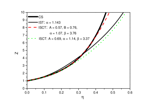
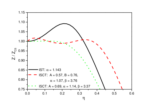
Figure 1: Left panel. Comparison of the compressibility factors $Z=\frac{p}{\rho T}$ of the CS EoS (solid thick curve) with the one-component IST EoS with best-fit parameters on interval of packing fraction $\eta\in[0.;0.4]$ (solid thin curve), the ISCT EoS with best-fit parameters on the same interval (dashed curve) and the ISCT EoS which exactly reproduces the five virial coefficients of the CS EoS (dotted curve). Right panel. Same as in the left panel, but for the ratios of the compressibility factors $Z/Z_{CS}$.

To reproduce five virial coefficients of the Monte-Carlo simulations for gas of hard-spheres[20]

$$Z_{MC}=1+4\eta+10\eta^{2}+18.36\eta^{3}+28.23\eta^{4}+39.74\eta^{5}+53.5\eta^{6}+70.8\eta^{7}$$ (19)

one should equate $a_{3}=10v^{2}$, $a_{4}=18.36v^{3}$ and $a_{5}=28.23v^{4}$ to the corresponding coefficients given by Eqs. (11)-(3). Then the solution with positive values of $\Sigma$ is

$$\gamma=0.316292v,\quad\delta=2.28784v,\quad\beta_{p}=0.298844\,.$$ (20)

Comparing the solutions (17) and (20) one can see that the difference between the coefficients is a few percent only.

4 Effective Excluded Volume and Effective Surface of Hard Spheres

   

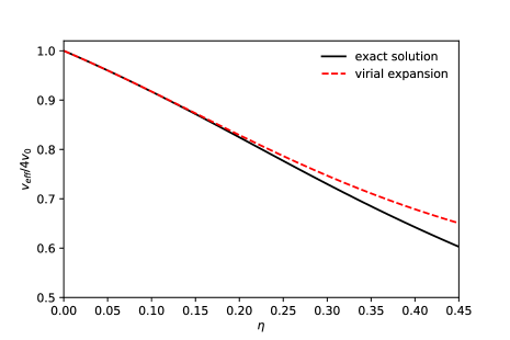
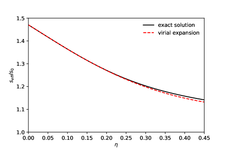
Figure 2: Left panel. Comparison of $\eta$ dependence of the effective excluded volume $v_{eff}$ (21) found from the ISCT EoS (solid curve) and from the virial expansion (6)-(8) for the solution (17) (dashed curve). Right panel. Same as in the left panel, but for the effective surface $s_{eff}$ (21).

Here we define the effective excluded volume $v_{eff}$ and effective surface $s_{eff}$ of particles

$$\frac{v_{eff}}{4v}=\frac{vp+s\Sigma+cK}{4vp}\,,\quad\frac{s_{eff}}{s}=1+\frac{cK}{s\Sigma},$$ (21)

as the density-dependent quantities. Fig. 2 explains the reason of why the ISCT EoS is more elaborate than the Van der Waals [1] and the IST EoS [10]. Indeed, the left panel of Fig. 2 demonstrates that in the ISCT EoS the effective excluded volume $v_{eff}$ sizably decreases if the particle number density grows, while in the Van der Waals the excluded volume is constant. Similarly, as one can see from the right panel of Fig. 2, the effective surface of particles $s_{eff}$ also decreases, if the particle number density grows, but in the IST EoS [10] the surface of particles is constant.

The density dependence of the effective excluded volume $v_{eff}$ can be used to develop the quantum EoS similar to the one suggested in Ref. 16, while the density-dependent effective surface of particles $s_{eff}$ may be useful to develop more realistic EoS of nuclear matter in which the total surface tension (being the sum of eigen surface tension and the induced one) of large nuclear fragments vanishes at the critical endpoint, as it should be.

5 Conclusions

In this work, we present the virial coefficients of the recently developed EoS based on the ISCT concept [15]. Besides the induced surface tension coefficient $\Sigma$ this concept takes into account the induced curvature tension coefficient $K$. Both tensions are generated by the hard-core repulsion of hard spheres. Similarly to the pressure $p$, the functions $\Sigma$ and $K$ also can be expanded into the virial expansion with the coefficients which are $T$-independent. The explicit expressions for the first five virial coefficients of $p$, $\Sigma$ and $K$ are presented here. They can be used for simple analytical estimates and development of more elaborate EoS of nuclear and neutron matters.

Appendix A Virial expansion coefficients

For the one-component ISCT EoS (1)-(3) we also found the virial coefficients for the surface tension coefficient $\Sigma$ (7)

$$b_{1}= 1\,,\quad b_{2}=4v-\gamma\,,$$ (22)

$$b_{3}= 16v^{2}+\frac{3\gamma^{2}}{2}+v\left(-14\gamma-6\delta\beta_{p}\right)\,,$$ (23)

$$b_{4}= 64v^{3}-\frac{8\gamma^{3}}{3}+v^{2}\left(-120\gamma-72\delta\beta_{p}\right)+v\left[\frac{87\gamma^{2}}{2}+\left(30\gamma\delta+\frac{27\delta^{2}}{2}\right)\beta_{p}\right]\,,$$ (24)

$$b_{5}= 256v^{4}+\frac{125\gamma^{4}}{24}+v^{3}\left(-832\gamma-576\delta\beta_{p}\right)+v^{2}(624\gamma^{2}+24\delta(26\gamma+9\delta)\beta_{p}$$

$$+ 72\delta^{2}\beta_{p}^{2})+v\left[\left(-111\gamma^{2}\delta-81\gamma\delta^{2}-32\delta^{3}\right)\beta_{p}-\frac{386\gamma^{3}}{3}\right]\,,$$ (25)

and the virial coefficients for the curvature tension coefficient $K$ (8)

$$c_{1}= 1\,,\quad c_{2}=4v-\gamma-\delta\,,$$ (26)

$$c_{3}= 16v^{2}+\frac{3\gamma^{2}}{2}+2\gamma\delta+\frac{3\delta^{2}}{2}+v\left(-14\gamma-8\delta-6\delta\beta_{p}\right)\,,$$ (27)

$$c_{4}= 64v^{3}-\frac{8\gamma^{3}}{3}-4\gamma^{2}\delta-\frac{9\gamma\delta^{2}}{2}-\frac{8\delta^{3}}{3}+v^{2}\left(-24(5\gamma+2\delta)-72\delta\beta_{p}\right)$$

$$+ v\left[\frac{87\gamma^{2}}{2}+36\gamma\delta+18\delta^{2}+\left(30\gamma\delta+\frac{51\delta^{2}}{2}\right)\beta_{p}\right]\,,$$ (28)

$$c_{5}= 256v^{4}+\frac{1}{24}\left(125\gamma^{4}+200\gamma^{3}\delta+270\gamma^{2}\delta^{2}+256\gamma\delta^{3}+125\delta^{4}\right)$$

$$+ v^{3}\left(-64(13\gamma+4\delta)-576\delta\beta_{p}\right)+v^{2}(48\left(13\gamma^{2}+8\gamma\delta+3\delta^{2}\right)$$

$$+ 24\delta(26\gamma+17\delta)\beta_{p}+72\delta^{2}\beta_{p}^{2})+v\left[\frac{1}{3}(-386\gamma^{3}-381\gamma^{2}\delta-297\gamma\delta^{2}\right.$$

$$- 128\delta^{3})+\left(-111\gamma^{2}\delta-153\gamma\delta^{2}-86\delta^{3}\right)\beta_{p}\biggl{]}\,.$$ (29)

References

- [1] J. D. van der Waals, Z. Phys. Chem. 5, 133 (1889).
- [2] V. V. Sagun, A. I. Ivanytskyi, K. A. Bugaev and I. N. Mishustin, Nucl. Phys. A 924, 24 (2014).
- [3] J. P. Bondorf et al., Phys. Rep. 257, 131 (1995) and references therein.
- [4] K. A. Bugaev et al., Nucl. Phys. A 970, 133 (2018).
- [5] V. V. Sagun et al., Eur. Phys. J. A 54, 100 (2018).
- [6] B. E. Grinyuk et al., arXiv:2004.05481v1 [hep-ph] (2020).
- [7] ALICE Collaboration (J. Adam et al.), Phys. Rev. C 93, 024917 (2016) and references therein.
- [8] ALICE Collaboration (L. Ramonaet al.), AIP Conf. Proc. 1701, (1) 080009 (2016) and references therein.
- [9] ALICE Collaboration (J. Adam et al.), Phys. Lett. B 754, 360 (2016) and references therein.
- [10] A. I. Ivanytskyi, K. A. Bugaev, V. V. Sagun, L. V. Bravina and E. E. Zabrodin, Phys. Rev. C 97, 064905 (2018).
- [11] P. Danielewicz, R. Lacey and W. G. Lynch, Science 298, 1593 (2002).
- [12] M. Dutra et al., Phys. Rev. C 90, 055203 (2014) and references therein.
- [13] K. A. Bugaev, A. I. Ivanytskyi, V. V. Sagun, E. G. Nikonov and G. M. Zinovjev, Ukr. J. Phys. 63, 863 (2018).
- [14] K. A. Bugaev, Eur. Phys. J. A 55, 215 (2019).
- [15] N. S. Yakovenko, K. A. Bugaev, L.V. Bravina and E. E. Zabrodin, arXiv:1910.04889 [nucl-th] p. 1-13.
- [16] V. Vovchenko, Phys. Rev. C 96, 015206 (2017)
- [17] N. F. Carnahan and K. E. Starling, J. Chem. Phys. 51, 635 (1969).
- [18] F. H. Stillinger, J. Chem. Phys. 128, 204705 (2008) and references therein.
- [19] C. Barrio and J. R. Solana, Phys. Rev. E 63, 011201 (2001).
- [20] M. N. Bannerman, L. Lue, and L. V. Woodcock, J. Chem. Phys. 132, 084507 (2010).
- [21] E. J. J. van Rensburg, J. of Physics A 26, 4805 (1993).