Bivectorial Nonequilibrium Thermodynamics:

Abstract

We generalize an idea in the works of Landauer and Bennett on computations, and Hill’s in chemical kinetics, to emphasize the importance of kinetic cycles in mesoscopic nonequilibrium thermodynamics (NET). For continuous stochastic systems, a NET in phase space is formulated in terms of cycle affinity $\nabla\wedge\big{(}{\bf D}^{-1}{\bf b}\big{)}$ and vorticity potential ${\bf A}({\bf x})$ of the stationary flux ${\bf J}^{*}=\nabla\times{\bf A}$. Each bivectorial cycle couples two transport processes represented by vectors and gives rise to Onsager’s notion of reciprocality; the scalar product of the two bivectors ${\bf A}\cdot\nabla\wedge\big{(}{\bf D}^{-1}{\bf b}\big{)}$ is the rate of local entropy production in the nonequilibrium steady state. An Onsager operator that relates vorticity to cycle affinity is introduced.

1 Introduction.

Nonequilibrium thermodynamics (NET) pioneered by L. Onsager onsager_reciprocal_1931 is concerned with a diverse array of macroscopic physical and chemical processes: mass transport, heat conduction, chemical reactions, etc. A unified treatment in continuous systems was developed in the 1960s groot_non-equilibrium_2011 . In recent years, introducing a NET of mesoscopic stochastic dynamics in its phase space has provided a more fundamental formulation in which the different physical and chemical fluxes are all represented by a single probability flux. Positivity of mean entropy production can be mathematically demonstrated, and large deviation fluctuation theorems were discovered lebowitz_gallavotti-cohen-type_1999 . The local equilibrium assumption required in groot_non-equilibrium_2011 does not enter the stochastic theory per se until its application when constitutive models for real world processes are required. In discrete-state systems, cycle flux and cycle affinity play fundamental roles in its NET; the initial idea goes back to hill_free_2012 . See qian_entropy_2016 for a recent synthesis.

2 Cycle completion and Irreversibility.

Consider the following thought experiment. Suppose we have a discrete-state Markov process and would like to determine whether its stationary process is detailed balanced or not, i.e. in equilibrium or not. We run the process with a trajectory $i_{0}i_{1}\cdots i_{k}$ and measure the dissipation

$$\mathcal{Q}(i_{0}i_{1}\cdots i_{k})=\ln\left(\frac{q_{i_{0}i_{1}}q_{i_{1}i_{2}}\cdots q_{i_{k-1}i_{k}}}{q_{i_{1}i_{0}}q_{i_{2}i_{1}}\cdots q_{i_{k}i_{k-1}}}\right)$$ (1)

where $q_{ij}$ is the (unknown) conditional transition rate from state $i$ to $j$. Komogorov’s cycle condition states that the process admits a detailed balanced steady state if and only if $\mathcal{Q}(\sigma)=0$ for all cycles $\sigma$, e.g. $i_{0}i_{1}\cdots i_{k}i_{0}$. Therefore, we shall examine $\mathcal{Q}$ everytime the process completes a cycle, and if $\mathcal{Q}=0$, we continue to run the process for another cycle. We can draw the conclusion either when we encouter a cycle with nonzero $\mathcal{Q}$, signifying detailed balance broken, or we complete all cycles and find that all cycles are reversible with zero dissipation.

In the thought experiment above, we see that it is essential to finish cycles to determine whether a system admits detailed balance or not. We can’t gain useful information before the process completes a full cycle. This is because for a trajectory one-step before the completion of a cycle, say $i_{0},i_{1},\cdots i_{k}$, with all distinct states, there’s always a possibility that the last step balances out the probability difference, i.e. $\mathcal{Q}(i_{0}i_{1}\cdots i_{k})+\mathcal{Q}(i_{k}i_{0})=0$, giving us a reversible cycle with no dissipation. We shall call this observation Landauer-Bennett-Hill (LBH) principle: In the theory of computation, R. Landauer applied the second law of thermodynamics to point out the necessary accompanied heat dissipation of “erasing one bit” landauer_irreversibility_1961 ; C. H. Bennett then used Landauer’s principle to argue that it is the last step of “erasing bits” in a cyclic Maxwell demon that “saves” the second law bennett_notes_2003 . Independently in the theory of cycle kinetics driven by chemostatic chemical potential, T. L. Hill introduced the concept of cycle completion hill_stochastics_1975 and argued that cycles in mesoscopic NET are more fundamental than transitions hill_free_2012 . The notion of “erasing one bit” of Landauer’s and Bennett’s matches exactly the idea of “completing one cycle”.

Parallel to the cycle representation of discrete-state Markov processes which has been extensively studied kalpazidou_cycle_2006 , here we present a cycle representation for the NET of continuous Markovian stochastic dynamics in its phase space the whole Euclidean $\mathbb{R}^{n}$, and discuss how the LBH principle comes in. The $n=2$ (and $n=3$ implied) case, in which a vector potential arises, has been investigated by one of the us qian_vector_1998 . However, the generalization to $n>3$ systems is nontrivial. One of the difficulties is that, for systems with $n>3$, vector calculus is no long sufficient since it is not possible to represent vorticity by a vector through the right-hand rule: there are more than one dimensions in the “thumb” direction. It turns out that both the cycle flux and cycle affinity in the continuous system are bivectors (see Appendix), which can be represented by their skew-symmetric $n\times n$ matrices components.

More importantly, while nonequilibrium steady state (NESS) cycle flux as a kinematic concept is nonlocal and requires highly nontrivial computation, the cycle affinity that quantifies NET thermodynamic driving force is locally determined and completely independent of the kinematics. The bivectorial nature of a cycle reflects the coupling between any two transport processes, visualizable as two vectors in $\mathbb{R}^{n}$, $X_{i}$ and $X_{j}$. This further implies the fundamental importance of cycles: a nonequilibrium device converts the force in $X_{i}$ to the transport in $X_{j}$, the two dimensions form a cycle and reciprocality naturally follows. In an equilibrium steady state, any clockwise and counter-clockwise fluxes on a cycle are exactly the same; thus Onsager’s reciprocal symmetry for NET in the linear regime follows. The bivector formalism helps establishing a clear physical picture and the mathematical representation of reciprocality in NET envisioned by Onsager.

3 Continuous Markov Processes.

Consider a mesoscopic system represented by a continuous Markov process with diffusion matrix ${\bf D}({\bf x})$ and drift ${\bf b}({\bf x})$, ${\bf x}\in\mathbb{R}^{n}$. Here we consider the dynamics on the whole Euclidean $\mathbb{R}^{n}$. The stochastic dynamics is described by a time-dependent probability density function $p({\bf x},t)$ that follows the Fokker-Planck equation (FPE)

$$\partial_{t}p({\bf x},t)=-\nabla\cdot\left[{\bf b}({\bf x})p({\bf x},t)-{\bf D}({\bf x})\nabla p({\bf x},t)\right].$$ (2)

With Ito’s calculus, this has a corresponding trajectory-based stochastic differential equation,

$${\rm d}\mathbf{X}_{t}=\left[{\bf b}\left(\mathbf{X}_{t}\right)+\nabla\cdot{\bf D}\left(\mathbf{X}_{t}\right)\right]{\rm d}t+\mathbf{\Gamma}\left(\mathbf{X}_{t}\right){\rm d}\mathbf{W}_{t}$$ (3)

where ${\bf D}=\mathbf{\Gamma}\mathbf{\Gamma}^{\mathsf{T}}/2$, $\left(\nabla\cdot{\bf D}\right)_{i}=\sum_{j=1}^{n}\partial_{j}D_{ji}$, and $\mathbf{W}_{t}$ is the $n$ dimensional Brownian motion. We’ve denoted $\partial_{j}$ as the partial derivative with respect to $x_{j}$.

With Eq. (2), the probability flux at $t$ is given by

$${\bf J}({\bf x},t)={\bf b}({\bf x})p({\bf x},t)-{\bf D}({\bf x})\nabla p({\bf x},t),$$ (4)

and the notion of “probability velocity” can be introduced as $\mathbf{v}({\bf x},t)={\bf J}\left({\bf x},t\right)/p({\bf x},t).$ In the stationary state, we have an invariant probability density $\pi({\bf x})$, a divergence-free stationary flux

$${\bf J}^{*}({\bf x})={\bf b}({\bf x})\pi({\bf x})-{\bf D}({\bf x})\nabla\pi({\bf x}),$$ (5)

and a “stationary probability velocity” $\mathbf{v}^{*}({\bf x})={\bf J}^{*}\left({\bf x}\right)/\pi({\bf x}).$ An equilibrium corresponds to detailed balanced condition: ${\bf J}^{*}({\bf x})=0=\mathbf{v}^{*}({\bf x})$.

4 Infinitesimal change and cyclic change of thermodynamic quantities.

Mesoscopic thermodynamics concerns the rate of change, production and dissipation of mainly three thermodynamic quantities: the (stochastic) Shannon entropy $S({\bf x},t)\coloneqq-\ln p({\bf x},t)$, the nonequilibrium potential energy $\Phi({\bf x})\coloneqq-\ln\pi({\bf x})$, and the free energy $F({\bf x},t)\coloneqq\Phi({\bf x})-S({\bf x},t)$ seifert_stochastic_2012 ; yang_unified_2020 . Their infinitesimal (stochastic) change along ${\bf X}_{t}$ from $t$ to $t+{\rm d}t$ can be expressed as

$$\mathrm{d}\Phi({\bf X}_{t}) =\nabla\Phi({\bf X}_{t})\circ\mathrm{d}\mathbf{X}_{t}$$ (6a)

$$\mathrm{d}S({\bf X}_{t},t) =\partial_{t}S({\bf X}_{t},t){\rm d}t+\nabla S\left({\bf X}_{t},t\right)\circ\mathrm{d}\mathbf{X}_{t}$$ (6b)

$$\mathrm{d}F({\bf X}_{t},t) =-\partial_{t}S({\bf X}_{t},t){\rm d}t+\nabla F\left({\bf X}_{t},t\right)\circ\mathrm{d}\mathbf{X}_{t}.$$ (6c)

Here $\circ$ denotes the Stratonovich midpoint integration: $\mathbf{u}(\mathbf{X}_{t},t)\circ\mathrm{d}\mathbf{X}_{t}$ is equal to $\mathbf{u}\left(\mathbf{X}_{t}+\tfrac{1}{2}\mathrm{d}\mathbf{X}_{t},t\right)\cdot\mathrm{d}\mathbf{X}_{t}$ which takes care of the extra term in Ito’s calculus due to the $\sqrt{{\rm d}t}$ scaling of $\mathrm{d}\mathbf{W}_{t}$ lebowitz_gallavotti-cohen-type_1999 ; qian_mesoscopic_2001 .

The instantaneous production of entropy ${\rm d}S$ has a decomposition ${\rm d}S={\mathchar 22\relax\mkern-12.0mu{\rm d}}\mathcal{S}_{\mathrm{tot}}-{\mathchar 22\relax\mkern-12.0mu{\rm d}}\mathcal{Q}$ in terms of the following two quantities,

$${\mathchar 22\relax\mkern-12.0mu{\rm d}}\mathcal{Q} ={\bf D}^{-1}{\bf b}\circ{\rm d}\mathbf{X}_{t}$$ (7a)

$${\mathchar 22\relax\mkern-12.0mu{\rm d}}\mathcal{S}_{\mathrm{tot}} =\partial_{t}S{\rm d}t+{\bf D}^{-1}\mathbf{v}\circ\mathrm{d}\mathbf{X}_{t}.$$ (7b)

They are the total amount of heat dissipated from the system to the environment lebowitz_gallavotti-cohen-type_1999 and the total entropy production of the system and the environment. Note the important distinction: Infinitesimal change of a function $A({\bf X}_{t},t)$ is ${\rm d}A\equiv A({\bf X}_{t+{\rm d}t},t+{\rm d}t)-A({\bf X}_{t},t)$; but there is no such a function for $\ {\mathchar 22\relax\mkern-12.0mu{\rm d}}\mathcal{B}$ in general. The latter represents work against a non-conservative force, or a “source” term. $\mathcal{B}$, or any calligraphic letter in the present work, is a path observable.

When the system reaches its NESS, the total entropy production at the steady state is the difference between the total heat dissipation $\thinspace{\mathchar 22\relax\mkern-12.0mu{\rm d}}\mathcal{Q}$ and the excess heat dissipation associated with the change in the nonequilibrium potential ${\mathchar 22\relax\mkern-12.0mu{\rm d}}\mathcal{Q}_{\mathrm{ex}}=-\nabla\Phi\circ\mathrm{d}\mathbf{X}_{t}.$ It is the amount of energy needed to sustain the steady state, called housekeeping heat,

$${\mathchar 22\relax\mkern-12.0mu{\rm d}}\mathcal{Q}_{\mathrm{hk}} \equiv{\mathchar 22\relax\mkern-12.0mu{\rm d}}\mathcal{Q}-{\mathchar 22\relax\mkern-12.0mu{\rm d}}\mathcal{Q}_{\mathrm{ex}}={\bf D}^{-1}\mathbf{v}^{*}\left(\mathbf{X}_{t}\right)\circ\mathrm{d}\mathbf{X}_{t}.$$ (8)

From Eqs (6c), (7a) and (8), one gets the entropy production decomposition $\thinspace{\mathchar 22\relax\mkern-12.0mu{\rm d}}\mathcal{S}_{\mathrm{tot}}={\mathchar 22\relax\mkern-12.0mu{\rm d}}\mathcal{Q}_{\mathrm{hk}}-{\rm d}F$. See yang_unified_2020 for a recent synthesis.

To compute the mean rate of the thermodynamic quantities above, we consider the infinitesimal change of a “work”-like quantity $\mathcal{W}$ associated with a “force” field $\mbox{\boldmath$f$}({\bf X}_{t},t)$,

$$\thinspace{\mathchar 22\relax\mkern-12.0mu{\rm d}}\mathcal{W}=\mbox{\boldmath$f$}({\bf X}_{t},t)\circ{\rm d}{\bf X}_{t}.$$ (9)

For a smooth cyclic path $\Gamma:\mathbf{x}(t),0\leq t\leq\tau$ where $\mathbf{x}(0)=\mathbf{x}(\tau)=\boldsymbol{\xi}$ in $\mathbb{R}^{n}$, the cyclic “work” can be rewritten by considering a surface $\Sigma$ whose boundary is given by the path $\Gamma$ and using Stoke’s theorem feng_potential_2011 .

$$\mathcal{W}(\Gamma) =\oint_{\Gamma}\mbox{\boldmath$f$}\cdot\mathrm{d}\mathbf{x}=\oint_{\Gamma}\sum_{i=1}^{n}f_{i}\mathrm{d}x_{i}$$ (10a)

$$=\int_{\Sigma}\sum_{1\leq i<j\leq n}\left(\partial_{i}f_{j}-\partial_{j}f_{i}\right)\mathrm{d}x_{i}\wedge\mathrm{d}x_{j}=\int_{\Sigma}\nabla\wedge\mbox{\boldmath$f$}\cdot\mathrm{d}\boldsymbol{\sigma}.$$ (10b)

In Eq. (10b), neither $\nabla\wedge\mbox{\boldmath$f$}$ nor $\mathrm{d}\boldsymbol{\sigma}$ are vectors in $\mathbb{R}^{n}$; rather they are bivectors, planary objects that have skew-symmetric matrix components with respect to the orthonormal basis $\{\mathbf{e}_{i}\wedge\mathbf{e}_{j},1\leq i<j\leq n\}$ where $\mathbf{e}_{i}$ is the unit vector in the $i$th direction of Cartesian coordinate and $\mathbf{e}_{i}\wedge\mathbf{e}_{j}$ is the signed area of the parallelogram spanned by $\mathbf{e}_{i}$ and $\mathbf{e}_{j}$. The $\nabla\wedge\mbox{\boldmath$f$}=\sum_{i<j}(\partial_{i}f_{j}-\partial_{j}f_{i})\mathbf{e}_{i}\wedge\mathbf{e}_{j}$ denotes the “curl” of $f$, representing the vorticity of $f$ by a bivector with skew-symmetric matrix components. Here, we understand $\mathrm{d}x_{i}\wedge\mathrm{d}x_{j}$ as the $(i,j)$th components of the infinitesimal plane $\mathrm{d}\boldsymbol{\sigma}$ as a bivector. The dot product in Eq. (10b) between two bivectors are defined as the half of the Frobenius product between their matrix components. See Appendix for a more detailed introduction in the language of differential form.

The cyclic changes of the thermodynamic quantities are then given by,

$$\Delta\Phi(\Gamma) =-\mathcal{Q}_{\mathrm{ex}}(\Gamma)=0$$ (11a)

$$\Delta S(\Gamma) =-\Delta F(\Gamma)=S(\boldsymbol{\xi},\tau)-S(\boldsymbol{\xi},0)$$ (11b)

$$\mathcal{Q}(\Gamma) =\mathcal{Q}_{\mathrm{hk}}(\Gamma)=\int_{\Sigma}\nabla\wedge\left({\bf D}^{-1}{\bf b}\right)\cdot\mathrm{d}\boldsymbol{\sigma}$$ (11c)

$$\mathcal{S}_{\mathrm{tot}}(\Gamma) =\Delta S(\Gamma)+\mathcal{Q}(\Gamma).$$ (11d)

If the path probability of a path $\Gamma$ in a Markov process starts with the invariant probability as the initial distribution, $\Delta S\left(\Gamma\right)=0$ for all cycles $\Gamma$, over which the total entropy production equals to the heat dissipation:

$$\mathcal{S}_{\mathrm{tot}}^{*}(\Gamma)=\mathcal{Q}(\Gamma)=\int_{\Sigma}\nabla\wedge\left({\bf D}^{-1}{\bf b}\right)\cdot\mathrm{d}\boldsymbol{\sigma}.$$ (12)

$S$ and $\Phi$ are state functions, but $\mathcal{Q}$ and $\mathcal{S}_{\mathrm{tot}}^{*}$ are not. These are direct consequences of (6) and (7a) in the cycle representation. In fact, Eq. (12) shows that $\nabla\wedge\left({\bf D}^{-1}{\bf b}\right)\cdot\mathrm{d}\boldsymbol{\sigma}$ is the cyclic entropy production of an infinitesimal cycle $\mathrm{d}\boldsymbol{\sigma}$, and the total cyclic entropy production is the integral of all the infinitesimal cycle that tiles the cycle $\Gamma$. This implies that the bivector $\nabla\wedge\left({\bf D}^{-1}{\bf b}\right)$ can be interpreted as the cycle affinity in diffusion, and the Komogorov’s cycle condition in diffusion for detailed balanced systems becomes a zero cycle affinity condition $\nabla\wedge\left({\bf D}^{-1}{\bf b}\right)=\mathbf{0}$. With Poicaré lemma applied on the contractible $\mathbb{R}^{n}$, this implies that ${\bf D}^{-1}{\bf b}$ is curl-free if and only if it is a gradient field, with a scalar potential given by $\Phi$.

Figure 1: Transitions on a infinitesimal square ${\rm d}x_{i}\wedge{\rm d}x_{j}$ in a lattice. The eight transition rates $q^{\pm}_{i\ \mathrm{or}\ j}$ determine the cycle affinity. This explains the physical picture of cycle affinity as shown in Eq. (13).

The physical picture of cycle affinity is clear in the discrete lattice picture as shown in Fig. 1. Focusing on the infinitesimal square of ${\rm d}x_{i}\wedge{\rm d}x_{j}$ at $x$, the cycle affinity of the counterclockwise cycle is given by

$$\mathcal{Q}_{ij} =\ln\frac{q_{i}^{+}(x)q_{j}^{+}(x+{\rm d}x_{i})q_{i}^{-}(x+{\rm d}x_{j})q_{j}^{-}(x)}{q_{i}^{-}(x)q_{j}^{-}(x+{\rm d}x_{i})q_{i}^{+}(x+{\rm d}x_{j})q_{j}^{+}(x)}$$ (13a)

$$\sim\left[\partial_{i}\left(\frac{1}{{\rm d}x_{j}}\ln\frac{q_{j}^{+}(x)}{q_{j}^{-}\left(x\right)}\right)-\partial_{j}\left(\frac{1}{{\rm d}x_{i}}\ln\frac{q_{i}^{+}(x)}{q_{i}^{-}\left(x\right)}\right)\right]{\rm d}x_{i}{\rm d}x_{j}.$$ (13b)

where $\frac{1}{{\rm d}x_{j}}\ln\frac{q_{j}^{+}}{q_{j}^{-}}$ becomes $\left({\bf D}^{-1}{\bf b}\right)_{j}$ from the theory of diffusion. We see that the particular order of $\partial_{i}\left({\bf D}^{-1}{\bf b}\right)_{j}-\partial_{j}\left({\bf D}^{-1}{\bf b}\right)_{i}$ is because the increment of $q_{j}^{+}/q_{j}^{-}$ in the $i$-th direction flavors the counterclockwise rotation whereas the increment of $q_{i}^{+}/q_{i}^{-}$ in the $j$-th direction hinders it. Their net contribution gives the force on the cycle, the cycle affinity.

The mean rate of $\mathcal{W}(t)$ in (10b) can be computed following Ito’s calculus qian_mesoscopic_2001 ,

$$\dot{\mathcal{W}}\equiv\frac{1}{\mathrm{{\rm d}t}}\mathbb{E}\left[\thinspace{\mathchar 22\relax\mkern-12.0mu{\rm d}}\mathcal{W}\right]=\int_{\mathbb{R}^{n}}{\bf J}(\mathbf{x},t)\cdot\mbox{\boldmath$f$}(\mathbf{x},t){\rm d}V$$ (14)

where ${\rm d}V=\prod_{i=1}^{n}{\rm d}x_{i}$ is the volume of a $n$-dimensional infinitesimal cube and $\mathbb{E}\left[\cdot\right]$ denotes expectation. The mean rates of $\Phi$, $S$, $F$, $\mathcal{S}_{\mathrm{tot}}$, and $\mathcal{Q}_{\mathrm{hk}}$ can then be obtained by plugging in the corresponding forces $\mbox{\boldmath$f$}=\nabla\Phi,\nabla S,\nabla F,\mathbf{D}^{-1}\mathbf{v}$, and $\mathbf{D}^{-1}\mathbf{v}^{*}$ yang_unified_2020 . We note that since $\mathbb{E}\left[\partial_{t}S\right]=0$, the first terms in Eqs. (6b) and (6c) do not contribute to the mean rate.

5 Cycle representation of kinematic NESS flux.

The divergence-free stationary flux $\mathbf{J}^{*}$ can be expressed in terms of a bivector potential ${\bf A}({\bf x})$ for diffusion on $\mathbb{R}^{n}$, $\nabla\times{\bf A}={\bf J}^{*}$. Note that ${\bf A}$ is also not a vector in $\mathbb{R}^{n}$ in general; rather it is a bivector whose components $A_{ij}$ satisfy

$$J_{i}^{*}({\bf x})=\left(\nabla\times{\bf A}\right)_{i}=\sum_{j=1}^{n}\partial_{j}A_{ij}({\bf x}).$$ (15)

It is straightforward to verify that $\nabla\cdot\left(\nabla\times{\bf A}\right)=0$. See Appendix for the derivation. Throughout the paper, we fix the $\times$ notation in $\nabla\times{\bf A}$ to denote the vector from a bivector potential ${\bf A}$, $(\nabla\times{\bf A})_{i}\coloneqq\sum_{j=1}^{n}\partial_{j}A_{ij}$, and the $\wedge$ notation in $\nabla\wedge\mathbf{u}$ to map a vector $\mathbf{u}$ to a bivector: $(\nabla\wedge\mathbf{u})_{ij}\coloneqq\partial_{i}u_{j}-\partial_{j}u_{i}$.

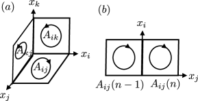
Figure 2: Bivector potential $A_{ij}$ and its derivative $\partial_{j}A_{ij}$ in a discrete lattice system. (a) For each unit vector $\hat{x}_{i}$ at a lattice point, there are $(n-1)$ number of $\hat{x}_{j}$ with which $\hat{x}_{i}\wedge\hat{x}_{j}$ forms a bivector, an oriented planar element. $A_{ij}$ is the cycle flux around the element. (b) $A_{ij}(n)-A_{ij}(n-1)$ contributes to the edge flux along $\hat{x}_{i}$. A similar $A_{ik}(m)-A_{ik}(m-1)$ also contributes to the same edge flux. This is the geometric meaning of Eq. (15).

The physical meaning of Eq. (15) is as followed. For every infinitesimal change $\mathrm{d}x_{i}$ in the $x_{i}$ direction at the point $\mathbf{x}\equiv(x_{1},\cdots,x_{n})\in\mathbb{R}^{n}$, there are $(n-1)$ orthogonal directions $\mathrm{d}x_{j}$, $j\neq i$, and $\mathrm{d}x_{i}\wedge\mathrm{d}x_{j}$ corresponds to a bivector, an infinitesimal planar element in the $ij$-th plane, as shown in Fig. 2(a). Here, we give the bivector potential $A_{ij}(\mathbf{x})$ a physical interpretation as the stationary cycle flux around the oriented infinitesimal planar element $\mathrm{d}x_{i}\wedge\mathrm{d}x_{j}$ at $\mathbf{x}$. The $i$th component of ${\bf J}^{*}$, $J_{i}^{*}$, is determined from all the neighboring infinitesimal planes $\mathrm{d}x_{i}\wedge\mathrm{d}x_{j}$, $j\neq i$. $\partial_{j}A_{ij}$ contributes a net edge flux along $x_{i}$ due to the pair of $A_{ij}$ at $(x_{1},\cdots,x_{j},\cdots,x_{n})$, and at $(x_{1},\cdots,x_{j}-\mathrm{d}x_{j},\cdots,x_{n})$ as shown in Fig. 2(b). An increasing $A_{ij}$ in the $j$th direction leads to a positive net flow $\partial_{j}A_{ij}$ in the $x_{i}$ direction. In a word, Eq. (15) gives a cycle representation of the steady state fluxes $J_{i}^{*}$ along the edges in terms of the cycle fluxes around the planar elements. An earlier discussion for 3-D cases can be found in qian_vector_1998 . ${\bf A}({\bf x})$ is a potential of ${\bf J}^{*}({\bf x})$ in terms of vorticity componenets at ${\bf x}$.

6 Landauer-Bennettt-Hill principle for diffusion.

In NESS, the ${\bf J}(\mathbf{x},t)$ in Eq. (14) is replaced by the divergence-free stationary flux ${\bf J}^{*}(\mathbf{x})$. With our bivector potential, the mean rate of $\mathcal{W}$ in Eq. (9) with corresponding force $f$ can be rewritten by integration by part,

$$\dot{\mathcal{W}}^{*}= \int_{\mathbb{R}^{n}}{\bf J}^{*}\cdot\mbox{\boldmath$f$}{\rm d}V=\int_{\mathbb{R}^{n}}\left(\nabla\times\mathbf{A}\right)\cdot\mbox{\boldmath$f$}{\rm d}V$$ (16a)

$$= \int_{\mathbb{R}^{n}}{\bf A}\cdot\left(\nabla\wedge\mbox{\boldmath$f$}\right){\rm d}V$$ (16b)

where the scalar product in Eq. (16a) is between two vectors whereas the scalar product in Eq. (16b) is between two bivectors, defined as the half Frobenius product of their antisymmetric matrix components . Importantly, Eq. (16b) gives the mean rate of $\mathcal{W}$ at NESS a new cyclic representation: it is the average of vorticity $\nabla\wedge\mbox{\boldmath$f$}$, weighted by the cycle flux ${\bf A}$. This immediately implies that thermodynamic quantities with a gradient force $-\nabla U$ would have zero mean rate in NESS since $\nabla\wedge\left(-\nabla U\right)=0$. That includes all the functions $\Phi$, $S$, and $F$, implying that the mean rates of $\mathcal{S}_{\mathrm{tot}}$, $\mathcal{Q}$, and $\mathcal{Q}_{\mathrm{hk}}$ are all identical at NESS, $\dot{\mathcal{S}}_{\mathrm{tot}}^{*}=\dot{\mathcal{Q}}^{*}=\dot{\mathcal{Q}}_{\mathrm{hk}}^{*}.$ This has been termed as a “gauge freedom” feng_potential_2011 ; polettini_nonequilibrium_2012 .

Thus, the average total entropy production rate at NESS can be written as

$$\dot{\mathcal{S}}_{\mathrm{tot}}^{*}= \int_{\mathbb{R}^{n}}{\bf A}\cdot\Big{[}\nabla\wedge({\bf D}^{-1}{\bf b})\Big{]}{\rm d}V.$$ (17)

The stationary cycle flux $\mathbf{A}$ is a purely kinematic concept that doesn’t have any thermodynamic content. A closed loop $\Gamma$ in $\mathbb{R}^{n}$ contains a surface $\Sigma$ which can be tiled by an array of tiny oriented infinitesimal planar elements at ${\bf x}$, for all ${\bf x}\in\Sigma$. ${\bf A}({\bf x})$ then decomposes ${\bf J}^{*}({\bf x})$, following Kirchhoff’s law, in terms of the occurrence rate of these tiny oriented elements along the infinitely long, ergodic path ${\bf X}_{t}$. As a vorticity description of the NESS, ${\bf A}$ is nonlocally determined.

On the other hand, as hinted by Eq. (12) and further by Eq. (17), the cycle affinity qian_entropy_2016 , as the Onsager’s thermodynamic force corresponding to the cycle flux, is locally determined through $\nabla\wedge\left({\bf D}^{-1}{\bf b}\right)$. ${\bf D}^{-1}{\bf b}$ should be identified as the vector potential of the cycle affinity. This is in sharp contrast to the standard expression $\dot{\mathcal{S}}_{\mathrm{tot}}^{*}=\int_{\mathbb{R}^{n}}{\bf J}^{*}\cdot{\bf D}^{-1}\mathbf{v}^{*}\mathrm{d}V$ where the thermodynamic force corresponding to the edge flux ${\bf J}^{*}$is nonlocally defined by ${\bf D}^{-1}{\bf v}^{*}$. Note that the cycle affinity has components

$$\left[\nabla\wedge\left({\bf D}^{-1}{\bf b}\right)\right]_{ij}=\partial_{i}({\bf D}^{-1}{\bf b})_{j}-\partial_{j}({\bf D}^{-1}{\bf b})_{i},$$ (18)

representing how the two dimensions $x_{i}$ and $x_{j}$ are coupled.

This constitutes the LBH principle for diffusion processes: Entropy production in NESS is characterized by the locally-defined cycle affinity as a bivector; entropy production of a bigger loop is the integral of the cycle affinity of infinitesimal cycles as shown in Eq. (12); and the average entropy production rate is the average cycle affinity, weighted by the cycle flux of infinitesimal cycles as shown in Eq. (17). The fundamental unit of NESS is the non-detailed-balanced kinetic cycle hill_free_2012 , in terms of bivectors.

7 Mean rate decomposition outside of NESS.

For the mean rate of thermodynamics quantities outside of NESS, we rewrite Eq. (14) as $\dot{\mathcal{W}}=\mathbb{E}\left[\mathbf{v}\left(\mathbf{X}_{t},t\right)\ \cdot\mbox{\boldmath$f$}\left(\mathbf{X}_{t},t\right)\right]$. By $\mathbf{v}({\bf x},t)=\mathbf{v}^{*}({\bf x})-{\bf D}\nabla F({\bf x},t),$ the mean rate has a decomposition,

$$\dot{\mathcal{W}}=\mathbb{E}\left[\mbox{\boldmath$f$}\cdot\mathbf{v}^{*}\right]-\mathbb{E}\left[\mbox{\boldmath$f$}\cdot{\bf D}\nabla F\right].$$ (19)

Outside of NESS, the two terms within can be rewritten as

$$\mathbb{E}\left[\mbox{\boldmath$f$}\cdot\mathbf{v}^{*}\right] =\int_{\mathbb{R}^{n}}{\bf A}\cdot\nabla\wedge\left(\frac{p}{\pi}\mbox{\boldmath$f$}\right){\rm d}V$$ (20a)

$$\mathbb{E}\left[\mbox{\boldmath$f$}\cdot{\bf D}\nabla F\right] =-\int_{\mathbb{R}^{n}}\frac{p}{\pi}\nabla\cdot\left(\pi{\bf D}\mbox{\boldmath$f$}\right){\rm d}V.$$ (20b)

This implies an average perpendicularity between $-\nabla F$ and $\mathbf{v}^{*}$, $\mathbb{E}[-\nabla F\cdot\mathbf{v}^{*}]=0.$

If with inner product defined as $\left\langle\mathbf{u},\mathbf{v}\right\rangle=\mathbb{E}\left[\mathbf{u}\cdot{\bf D}^{-1}\mathbf{v}\right]$, this average perpendicularity becomes $\left\langle-{\bf D}\nabla F,\mathbf{v}^{*}\right\rangle=0$. The decomposition in Eq. (19) has a geometric interpretation under the provided inner product. The mean rate of a “work”-like quantity $\mathcal{W}$ of Eq. (9) with the force $f$ is determined by the inner product of ${\bf D}\mbox{\boldmath$f$}$ with two perpendicular vectors, $\mathbf{v}^{*}$ and $-{\bf D}\nabla F$,

$$\dot{\mathcal{W}}=\left\langle{\bf D}\mbox{\boldmath$f$},\mathbf{v}^{*}\right\rangle+\left\langle{\bf D}\mbox{\boldmath$f$},-{\bf D}\nabla F\right\rangle.$$ (21)

This gives the Pythogarean-like relation between $\mathbf{v}$, $\mathbf{v}^{*}$, and $-{\bf D}\nabla F$ qian_kinematic_2020 hidden behind the famous entropy production rate decomposition ge_extended_2009 ,

$$\underbrace{\left\langle\mathbf{v},\mathbf{v}\right\rangle}_{\dot{\mathcal{S}}_{\mathrm{tot}}} =\underbrace{\left\langle\mathbf{v}^{*},\mathbf{v}^{*}\right\rangle}_{\dot{\mathcal{Q}}_{\mathrm{hk}}}+\underbrace{\left\langle-{\bf D}\nabla F,-{\bf D}\nabla F\right\rangle}_{\dot{F}_{\mathrm{d}}}.$$ (22)

Results above indicate that $\mathbf{v}^{*}$ and $-{\bf D}\nabla F$ originate from two rather disjoint irreversibilities, and that the geometry defined through the Riemannian metric $\mathbf{D}^{-1}(\mathbf{x})$ may be the most natural one in thermodynamics.

8 Onsager’s reciprocality and the Onsager operator.

A diffusion process in $\mathbb{R}^{n}$ always has its NESS thermodynamic force $\mathbf{D}^{-1}\mathbf{v}^{*}$ linearly related to transport flux ${\bf J}^{*}$, $\left(\mathbf{D}^{-1}\mathbf{v}^{*}\right)_{i}$ $=e^{\Phi}\sum_{j=1}^{n}D_{ij}^{-1}J_{j}^{*}$. Many previous studies have explored this unique feature qian_mesoscopic_2001 ; reguera_mesoscopic_2005 . In the bivectorial representation there is a further linear affinity-vorticity relationship

$$\nabla\wedge\left({\bf D}^{-1}{\bf b}\right)({\bf x}) =\mathcal{O}{\bf A}({\bf x}).$$ (23)

where $\mathcal{O}=\nabla\wedge\left(e^{\Phi}{\bf D}^{-1}\nabla\times\right)$. We shall call the operator $\mathcal{O}$ the Onsager operator. It linearly relates the cycle flux bivector to the cycle affinity bivector. As an example for the Onsager operator superimposing different ${\bf A}$ from different processes, we note that $(\Phi,\mathbf{A},\mathbf{D})$ together specify a diffusion process on $\mathbb{R}^{n}$ with $\Phi$ and ${\bf A}$ as the scalar and bivector potentials of ${\bf b}$. Therefore, for a family of systems with fixed $\Phi$ and ${\bf D}$, different bivector potential ${\bf A}$ gives us different processes. With $\mathcal{O}$ fixed in a family, a third process in this family with ${\bf A}_{3}={\bf A}_{1}+{\bf A}_{2}$ will have cycle affinity $\mathcal{O}{\bf A}_{3}=\mathcal{O}\left({\bf A}_{1}+{\bf A}_{2}\right)=\mathcal{O}{\bf A}_{1}+\mathcal{O}{\bf A}_{2}$. With in this family, $(\Phi,\mathbf{0},\mathbf{D})$ is a reversible process; and $(\Phi,-\mathbf{A},\mathbf{D})$ is the adjoint process.

Figure 3: Two edges $\eta$ and $\eta^{\prime}$ are coupled through all the cycles $\gamma$ they are both in. The cycle-coupling is the origin of Onsager’s reciprocality. Arrows represent cycle edges, and line with dot at the end represents the driving from force to flux. Dash lines indicate the smallest cycle coupling and solid lines indicate another cycle coupling.

For discrete-state systems, it was understood in hill_linear_1982 ; qian_entropy_2016 that such a relation at the cycle level is the fundamental origin of the Onsager’s reciprocality and symmetry. Specifically, if we denote $G_{\gamma\eta}$ as the incidence matrix of an edge $\eta$ in a cycle $\gamma$, then the stationary net edge flux is coupled with other edges through cycles,

$$J_{\eta}=\sum_{\gamma\in\mathrm{all\ cycles}}G_{\gamma\eta}J_{\gamma}^{-}\left[\exp\left(\sum_{\eta^{\prime}}G_{\gamma\eta^{\prime}}\mathcal{Q}(\eta^{\prime})\right)-1\right]$$ (24)

where $J_{\gamma}^{-}$ is the one-way cycle flux with orientation reversed to $\gamma$. The reciprocality between $\eta$ and $\eta^{\prime}$ manifests in that the mutual interaction between them are coupled only through cycles that contain both $\eta$ and $\eta^{\prime}$: Among all cycles, only those which contains $\eta$ contribute to $J_{\eta}$; among them, only those which contains $\eta^{\prime}$ has the effect from $\eta^{\prime}$, i.e. a $\mathcal{Q}(\eta^{\prime})$ term in $(\cdots)$; and only among these shared cycles does $\mathcal{Q}({\eta})$ affect back to $J_{\eta^{\prime}}$, as illustrated by Fig. 3. The symmetry of the reciprocality further requires the system to be near equilibrium in general discrete-systems. With $J^{\mathrm{eq}}_{\gamma}$ denoting the equilibrium one-way flux, $J_{\gamma}^{-}\simeq J^{\mathrm{eq}}_{\gamma}$, and the cycle affinity to be small near equilibrium $\mathcal{Q}_{\gamma}\ll 1$ for all cycle $\gamma$, Eq. (24) becomes, to-the-leading-order,

$$J_{\eta}\simeq\sum_{\eta^{\prime}}\left(\sum_{\gamma\in\mathrm{all\ cycles}}G_{\gamma\eta}J^{\mathrm{eq}}_{\gamma}G_{\gamma\eta^{\prime}}\right)\mathcal{Q}_{\eta^{\prime}}$$ (25)

with symmetric Onsager matrix given by $\left(\cdots\right)$.

The bivectorial cycles in diffusion processes demonstrates vividly the reciprocality between two dimensions. How treating a diffusion process as a discrete-state Markov process on infinitesimal lattice system could reveal the fundamental origin of the general force-flux linearity and the symmetry in the Onsager’s reciprocality for systems even far away from equilibrium remain to be ellucinated in future works. We note that the mean NESS entropy production rate has a simple bilinear form:

$$\dot{\mathcal{S}}_{\mathrm{tot}}^{*} =\int_{\mathbb{R}^{n}}{\bf A}\cdot\mathcal{O}{\bf A}{\rm d}V.$$ (26)

Incidentally, Onsager also considered tiny vortices “who wanted to play” as the fundamental objects in hydrodynamic turbulent flow eyink_onsager_2006 .

9 The probabilistic gauge of the bivector potential ${\bf A}$.

The bivector potential ${\bf A}$ obtained for the divergence-free ${\bf J}^{*}({\bf x})=\nabla\times{\bf A}({\bf x})$ is not unique: It has a gauge freedom with an arbitrary curl-free bivector. The situation has an analogue to that of discrete-state Markov process qian_decomposition_1979 ; qian_circulation_1982 , and the vector potential in classical electrodynamics. Interestingly, for discrete-state Markov process, Qian and Qian have proven the existence and uniqueness of a gauge with a probabilistic meaning: Cycles are not just represented in terms of Kirchhoff decomposition via linearly independent bases; rather the space of all possible cycles are considered, on which the unique probabilistic gauge, as NESS cycle flux, is the occurrence rate of a given cycle along the infinitely long, ergodic path qian_circulation_1982 . Whether such a unique probabilistic gauge also exists for bivector potential ${\bf A}$ on $\mathbb{R}^{n}$, or a more extended space of loops lejan_2010 , remains to be further investigated.

10 Conclusions and discussion.

This study clearly points to the importance of cycle representation for mesoscopic nonequilibrium thermodynamics (NET) in terms of cycle flux ${\bf A}$ and cycle affinity $\nabla\wedge\big{(}{\bf D}^{-1}{\bf b}\big{)}$. The former is a pure kinematic concept and the latter contains all the fundamental information on NET. We show that the cycle flux and cycle affinity are not simple vectors in $\mathbb{R}^{n}$; rather they are bivectors, which can be represented by skew-symmetric matrices. The cycle flux is the bivector potential of the conventional NESS flux; and the cycle affinity has a vector potential ${\bf D}^{-1}({\bf x}){\bf b}({\bf x})$ which is obtained locally.

Some of the mathematics in the present work is contained in the diffusion process on a manifold qian_entropy_1999 and the gauge field formulations of NET feng_potential_2011 ; polettini_nonequilibrium_2012 . The present work provides a clearer physics of NET in phase space as a formulation of Onsager’s general principle for entropy production. We identify the bivector nature of the cycle representation in terms of a local cycle affinity and a nonlocal kinematic cycle flux; and reveal a unified Landauer-Bennett-Hill thermodynamic principle for stationary nonequilibrium systems.

Finally, we noted a parallel between quantum mechanical phase giving a reality to the “indeterminate” vector potential in electromagnetism wu_evolution_2006 and our stochastic formulation giving a vorticity intepretation to the bivector ${\bf A}$ in stochastic thermodynamics: Steady state flux ${\bf J}^{*}$ turns out to be a derivative.

Conflict of interest

This work is partially supported by the Olga Jung Wan Endowed Professorship for the second author. The authors have no conflicts of interest to declare that are relevant to the content of this article.

Appendix

Here we summarize the mathematics used to derive the results in the present work. In the main text, we used the notion of multivariable calculus and the notion of wedge product without the introduction of differential form for simplicity. However, the concept of differential form and the associated exterior calculus are needed to derive the formula of generalized curl and cross product for dimensions higher than $3$ arnold_mathematical_1997 ; fortney_visual_2018 . We shall introduce and use the differential form calculus here. Throughout the text, we will use Cartesian coordinate to describe the entire Euclidean $\mathbb{R}^{n}$.

A. Differential form and Integration

In vector calculus, the infinitesimal work done by a force $f$ from time $t$ to $t+\delta t$ on a path ${\bf y}(t)$ is given by

$$\delta\mathcal{W}=\mbox{\boldmath$f$}({\bf y}(t))\cdot\delta{\bf y}(t)=\sum_{j=1}^{n}f_{j}({\bf y}(t))\delta y_{j}(t+\delta t)$$ (A 1)

where $\delta{\bf y}(t)$ denotes the infinitesimal vector ${\bf y}(t+\delta t)-{\bf y}(t)$. Usually, to emphasize the infinitesimal limit $\delta t\rightarrow 0$, we replace $\delta$ with ${\rm d}$, leading to a notation $\mbox{\boldmath$f$}({\bf y}(t))\cdot{\rm d}{\bf y}(t)$. However, in the mathematics of differential form, the operater ${\rm d}$ is generalized and understood differently. In the main text, we used ${\rm d}$ as the standard infinitesimal difference operator in calculus. Here, we shall use $\delta$ as the infinitesimal operator and ${\rm d}$ as the exterior derivative of differential form, as we will introduce below.

We first introduce the concept of 1-forms, which are linear functions that maps a vector to a real number. Notice that the infinitesimal work in Eq. (A 1) actually takes the (tangent) vector $\delta{\bf y}(t)$ at a point ${\bf y}(t)$ and return us a number. The infinitesimal work is thus generally a differential 1-form at a given point, say $\boldsymbol{\xi}$, associated with a force vector $\mbox{\boldmath$f$}=(f_{1},f_{2},\cdots,f_{n})$,

$$\omega_{\boldsymbol{\xi}}({\bf u})=\sum_{j=1}^{n}f_{j}(\boldsymbol{\xi}){\rm d}x_{j}({\bf u}).$$ (A 2)

It takes an infinitesimal vector ${\bf u}$ as an input and gives us the infinitesimal work generated when going from $\boldsymbol{\xi}$ to $\boldsymbol{\xi}+{\bf u}$. The basis of a 1-form is $\{{\rm d}x_{j}\}$, which are themselves 1-forms: ${\rm d}x_{i}$ takes a vector ${\bf u}$ and gives us its $i$th component,

$${\rm d}x_{i}\left(\sum_{j}u_{j}\mathbf{e}_{j}\right)=\mathbf{e}_{i}\cdot\left(\sum_{j}u_{j}\mathbf{e}_{j}\right)=u_{i}$$ (A 3)

where $\mathbf{e}_{i}$ is the unit vector in the $i$th direction. To match up Eq. (A 1) with Eq. (A 2), simply take ${\bf u}\coloneqq\delta{\bf y}(t)$ and $\boldsymbol{\xi}={\bf y}(t)$. The relation ${\rm d}x_{i}(\square)=\mathbf{e}_{i}\cdot\square$ is what allows us to write the differential form in a vectorized expression in the main text,

$$\omega_{\boldsymbol{\xi}}({\bf u}) =\sum_{i}f_{i}(\boldsymbol{\xi}){\rm d}x_{i}\left(\sum_{j}u_{j}\mathbf{e}_{j}\right)$$ (A 4a)

$$=\sum_{i}f_{i}(\boldsymbol{\xi})\mathbf{e}_{i}\cdot\left(\sum_{j}u_{j}\mathbf{e}_{j}\right)=\mbox{\boldmath$f$}(\boldsymbol{\xi})\cdot{\bf u}.$$ (A 4b)

A differential form is what we can integrate over a manifold. The integral of the work over a path $\Gamma=\{{\bf y}(s),0\leq s\leq t\}$ is then

$$\int_{\Gamma}\omega=\int_{\Gamma}\sum_{j=1}^{n}f_{j}{\rm d}x_{j}=\int_{0}^{t}\sum_{j=1}^{n}f_{j}(\boldsymbol{{\bf y}}(s)){\rm d}x_{j}(\delta{\bf y}(s))$$ (A 5)

where inputs of the differential form are suppressed concisely before the parameterization in the last step. To carry out the computation, one would proceed with ${\rm d}x_{j}(\delta{\bf y}(s))=\delta{\bf y}_{j}(s)={\bf y}_{j}^{\prime}(s){\rm d}s$, which makes Eq. (A 5) an usual one dimensional integration w.r.t. $s$. This identification of differential form turns out to be significant for the general integral of $m$-form on a general manifold and the generalization of Stoke’s theorem.

B. Bivector and 2-form

Stokes theorem in $\mathbb{R}^{3}$ tells us that a line integral of a vector field on a closed loop is equal to the surface integral of the vector field’s curl. The intuition behind is that the curl of the vector field gives the vorticity of the vector field of an infinitesimal plane object. When integrating all the infinitesimal planes that tile the surface, neighboring circulation cancels and all the vorticity of the infinitesimal plane combines to give the vorticity on the big loop on the boundary. This intuition is still valid in $\mathbb{R}^{n}$. To see that, we shall first introduce how the “planary object” is represented in general $\mathbb{R}^{n}$: it is given by the notion of a (simple) bivector.

Two parameters are needed to parametrize a surface, and a surface can be cut into infinitesimal two dimensional parallelograms with edges given by the two infinitesimal tangent vectors of a point. Moreover, circulation of a vector field over an infinitesimal plane can have two orientations. Putting these together, we use the notion ${\bf u}\wedge{\bf v}$ to represent an oriented parallelogram object spanned by two vectors ${\bf u}$ and ${\bf v}$, thus the name bivector. The orientation of the object is reflected by the anti-symmetry of the wedge product $\wedge$, ${\bf u}\wedge{\bf v}=-{\bf v}\wedge{\bf u}$. The wedge product $\wedge$ is a linear operation satisfying $(c_{1}{\bf u}_{1}+c_{2}{\bf u}_{2})\wedge{\bf v}=c_{1}{\bf u}_{1}\wedge{\bf v}+c_{2}{\bf u}_{2}\wedge{\bf v}$ where $c_{1},c_{2}\in\mathbb{R}$. With these, we can get the component form of the bivector

$${\bf u}\wedge{\bf v}=\sum_{1\leq i<j\leq n}(u_{i}v_{j}-u_{j}v_{i})\mathbf{e}_{i}\wedge\mathbf{e}_{j}$$ (A 6)

with basis $\mathbf{e}_{i}\wedge\mathbf{e}_{j}$. Importantly, one can show that the area of the parallelogram, denoted as $\|{\bf u}\wedge{\bf v}\|$ is given by

$$\|{\bf u}\wedge{\bf v}\|^{2}=\sum_{1\leq i<j\leq n}(u_{i}v_{j}-u_{j}v_{i})^{2}.$$ (A 7)

An inner product between two bivectors $\mathbf{A}=\sum_{i<j}A_{ij}\mathbf{e}_{i}\wedge\mathbf{e}_{j}$ and $\mathbf{B}=\sum_{i<j}B_{ij}\mathbf{e}_{i}\wedge\mathbf{e}_{j}$ is thus naturally defined as

$$\mathbf{A}\cdot\mathbf{B}=\sum_{1\leq i<j\leq n}A_{ij}B_{ij}$$ (A 8)

with $\left(\mathbf{e}_{i}\wedge\mathbf{e}_{j}\right)\cdot\left(\mathbf{e}_{k}\wedge\mathbf{e}_{l}\right)=\delta_{ik}\delta_{jl}$ for $i<j$ and $k<l$.

We note that, in general, bivectors are objects that can be expressed as $\mathbf{A}=\sum_{i<j}A_{ij}\mathbf{e}_{i}\wedge\mathbf{e}_{j}$. Not all bivector can be expressed as the wedge product of two vectors. Such bivectors are called simple bivectors, and only simple bivectors can have the geometrical meaning as a parallelogram spanned by two vectors: a general bivector can be the sum of many simple bivectors, superposition of many parallelogram. We also note that due to the anti-symmetry of the wedge product, the component $A_{ij}$ of a bivector ${\bf A}$ can be represented by an anti-symmetric matrix. Then, the inner product between two bivectors, as shown in Eq. (A 8), is the half of the Frobenius product of their anti-symmetric components.

Now, similar to a 1-form taking a vector to a real number, a 2-form takes a bivector to a real number.The basis of a 2-form is given by $\{{\rm d}x_{i}\wedge{\rm d}x_{j}\}$ for $1\leq i<j\leq n$. Specifically, for $1\leq i<j\leq n$,

$${\rm d}x_{i}\wedge{\rm d}x_{j}\left(\sum_{k<l}A_{kl}\mathbf{e}_{k}\wedge\mathbf{e}_{l}\right)=\left(\mathbf{e}_{i}\wedge\mathbf{e}_{j}\right)\cdot\left(\sum_{k<l}A_{kl}\mathbf{e}_{k}\wedge\mathbf{e}_{l}\right)=A_{ij}.$$ (A 9)

Again, the relation between ${\rm d}x_{i}\wedge{\rm d}x_{j}\left(\mathbf{A}\right)=\left(\mathbf{e}_{i}\wedge\mathbf{e}_{j}\right)\cdot\mathbf{A}$ is what allow us to rewrite a differential 2-form in a vectorized form in the main text,

$$\omega(\mathbf{A}) =\sum_{i<j}B_{ij}{\rm d}x_{i}\wedge{\rm d}x_{j}\left(\mathbf{A}\right)=\sum_{i<j}B_{ij}\left(\mathbf{e}_{i}\wedge\mathbf{e}_{j}\right)\cdot\mathbf{A}$$ (A 10a)

$$=\sum_{i<j}B_{ij}A_{ij}=\mathbf{B}\cdot\mathbf{A}.$$ (A 10b)

When integration the differential 2-form over a surface, the $\mathbf{A}$ as the input of the 2-form here would be the infinitesimal bivector given by the two infinitesimal tangent vectors at a point, representing the infinitesimal tangent parallelogram at the point.

C. Exterior Derivative and the Curl of a vector field

The concept of curl in vector calculus is useful because of the Stokes theorem in $\mathbb{R}^{3}$. We shall thus use the generalized version of the Stokes theorem, the Stoke-Cartan theorem, to motivate the notion of exterior derivative and get the general definition of the curl of a vector field in $\mathbb{R}^{n}$.

The Stokes-Cartan theorem states that the integral of a differential form $\omega$ over the boundary of some oriented manifold $\Omega$ is equal to the integral of its exterior derivative ${\rm d}\omega$ over the whole of $\Omega$:

$$\oint_{\partial\Omega}\omega=\int_{\Omega}{\rm d}\omega.$$ (A 11)

In a sense, the exterior derivative ${\rm d}$ is defined so that Eq. (A 11) holds for a general manifold. We shall thus understand it with Stokes-Cartan theorem: the exterior derivative of a differential form $\omega$ can be interpreted, geometrically, as the integral over the boundary of an infinitesimal parallelepiped $h\Omega$,

$${\rm d}\omega=\lim_{h\rightarrow 0}\frac{1}{\|h\Omega\|}\int_{\partial(h\Omega)}\omega$$ (A 12)

where $\|h\Omega\|$ denotes the volume of $h\Omega$. With this, one sees that the twice exterior derivative of any differential form has to be zero, ${\rm d}{\rm d}\omega=0$. This is by applying the Stokes-Cartan theorem twice for a form that is itself the exterior derivative of another form $\varphi={\rm d}\omega$ (such form is called exact). For an arbitrary compact region $\Omega$, we have

$$\int_{\Omega}{\rm d}{\rm d}\omega=\int_{\Omega}{\rm d}\varphi=\int_{\partial\Omega}\varphi=\int_{\partial\Omega}{\rm d}\omega=\int_{\partial\partial\Omega}\omega.$$ (A 13)

Since $\partial\partial\Omega=\emptyset$ and $\Omega$ is arbitrary, we have ${\rm d}{\rm d}\omega=0$. A form with zero exterior derivative is said to be closed. Therefore, every exact form is closed.

The exterior derivative of a $k$-form is a $(k+1)$-form. The exterior derivative of a general form $\alpha\wedge\beta$ obeys the product rule: Suppose $\alpha$ is a $p$-form, then

$${\rm d}\left(\alpha\wedge\beta\right)={\rm d}\alpha\wedge\beta+\left(-1\right)^{p}\left(\alpha\wedge{\rm d}\beta\right).$$ (A 14)

Applying this and ${\rm d}{\rm d}\omega=0$, one can get the exterior derivative of the 1-form in Eq. (A 2),

$${\rm d}\left(\sum_{j=1}^{n}f_{j}{\rm d}x_{j}\right) =\sum_{j=1}^{n}\left({\rm d}f_{j}\right)\wedge{\rm d}x_{j}=\sum_{1\leq i,j\leq n}\left(\frac{\partial f_{j}}{\partial x_{i}}{\rm d}x_{i}\right)\wedge{\rm d}x_{j}$$ (A 15a)

$$=\sum_{1\leq i<j\leq n}\left(\frac{\partial f_{j}}{\partial x_{i}}-\frac{\partial f_{i}}{\partial x_{j}}\right){\rm d}x_{i}\wedge{\rm d}x_{j}$$ (A 15b)

where ${\rm d}x_{i}\wedge{\rm d}x_{j}=-{\rm d}x_{j}\wedge{\rm d}x_{i}$ is used. By Stokes-Cartan theorem, we the have

$$\oint_{\partial\Omega}\sum_{j=1}^{n}f_{j}{\rm d}x_{j}=\int_{\Omega}\sum_{1\leq i<j\leq n}\left(\frac{\partial f_{i}}{\partial x_{j}}-\frac{\partial f_{i}}{\partial x_{j}}\right){\rm d}x_{i}\wedge{\rm d}x_{j}.$$ (A 16)

As introduced in Sec. B, we can rewrite Eq. (A 16) in the vectorized form,

$$\oint_{\partial\Omega}\mbox{\boldmath$f$}\cdot{\rm d}{\bf x}=\int_{\Omega}\nabla\wedge\mbox{\boldmath$f$}\cdot{\rm d}\boldsymbol{\sigma}$$ (A 17)

where inner product between bivectors was introduced in Eq. (A 8). Hence, $\nabla\wedge\mbox{\boldmath$f$}$ as a bivector is the curl of the vector field $f$.

Since ${\rm d}{\rm d}\omega=0$, a gradient vector field is always curl-free, i.e. $\nabla\wedge\nabla U=0$ where $U$ is a scalar potential. For the converse, we apply Poicaré lemma, which states that every closed form is exact (locally) on a contractible domain. Since we are concern with processes on the entire Euclidean manifold $\mathbb{R}^{n}$, which is contractible, we can conclude that curl-free vector field is globally a gradient field.

D. Bivector potential of a divergence-free vector field

Using exterior derivatives and differential forms, the integral of a vector field ${\bf F}({\bf x})$ over an $(n-1)$-dimensional closed surface $\Sigma$ as flux is

$$\oint_{\Sigma}\sum_{k=1}^{n}F_{k}({\bf x}){\rm d}\sigma_{k} =\int_{\Omega}{\rm d}\left(\sum_{k=1}^{n}F_{k}({\bf x}){\rm d}\sigma_{k}\right)$$ (A 18a)

$$=\int_{\Omega}\sum_{k=1}^{n}\left[\sum_{j=1}^{n}\left(\partial_{j}F_{k}\right){\rm d}x_{j}\right]\wedge{\rm d}\sigma_{k}$$ (A 18b)

$$=\int_{\Omega}\sum_{k,j=1}^{n}\left(\partial_{j}F_{k}\right){\rm d}x_{j}\wedge{\rm d}\sigma_{k}$$ (A 18c)

$$=\int_{\Omega}\sum_{j=1}^{n}\left(\partial_{j}F_{j}\right){\rm d}V,$$ (A 18d)

where $\Omega$ is the $n$-volume contained by the closed $(n-1)$-surface $\Sigma$, and

$${\rm d}\sigma_{k}=(-1)^{k-1}{\rm d}x_{1}\wedge{\rm d}x_{2}\wedge\cdots\wedge{\rm d}x_{k-1}\wedge{\rm d}x_{k+1}\wedge\cdots\wedge{\rm d}x_{n}$$ (A 19)

with ${\rm d}x_{k}$ missing. The $(-1)^{k-1}$ factor is to ensure ${\rm d}x_{j}\wedge{\rm d}\sigma_{k}=\delta_{jk}{\rm d}V$ where

$${\rm d}V={\rm d}x_{1}\wedge{\rm d}x_{2}\wedge\cdots\wedge{\rm d}x_{n}$$ (A 20)

is the infinitesimal $n$ dimensional volume element. The $(n-1)$-form ${\rm d}\sigma_{i}$ is the Hodge dual of the 1-form ${\rm d}x_{i}$, often denoted as ${\rm d}\sigma_{i}=\star{\rm d}x_{i}$.

Now if a vector field ${\bf F}({\bf x})$ is divergence free, i.e. $\sum_{j=1}^{n}\left(\partial_{j}F_{j}\right)=0$, then the $(n-1)$-form has a zero exterior derivative,

$${\rm d}\left(\sum_{k=1}^{n}F_{k}({\bf x}){\rm d}\sigma_{k}\right)=0.$$ (A 21)

Poicaré lemma then guarantees that on a contractible domain,

$$\sum_{k=1}^{n}F_{k}({\bf x}){\rm d}\sigma_{k}={\rm d}\omega,$$ (A 22)

where $\omega$ is expected to be a $(n-2)$-form with the general expression

$$\omega=\sum_{1\leq i<j\leq n}u_{ij}({\bf x}){\rm d}\eta_{ij},$$ (A 23)

in which

$${\rm d}\eta_{ij}=(-1)^{i-1+j-2}{\rm d}x_{1}\cdots{\rm d}x_{i-1}\wedge{\rm d}x_{i+1}\wedge\cdots{\rm d}x_{j-1}\wedge{\rm d}x_{j+1}\cdots{\rm d}x_{n}$$ (A 24)

with ${\rm d}x_{i}$ and ${\rm d}x_{j}$ missing. The $(-1)^{i-1+j-2}$ factor is to ensure $\left({\rm d}x_{i}\wedge{\rm d}x_{j}\right)\wedge{\rm d}\eta_{ij}={\rm d}V$ so that ${\rm d}\eta_{ij}=\star\left({\rm d}x_{i}\wedge{\rm d}x_{j}\right)$. Then,

$${\rm d}\omega =\sum_{1\leq i<j\leq n}\sum_{k=1}^{n}\left(\partial_{k}u_{ij}\right){\rm d}x_{k}\wedge{\rm d}\eta_{ij}$$ (A 25a)

$$=\ \sum_{1\leq i<j\leq n}\left\{\left(\partial_{i}u_{ij}\right){\rm d}x_{i}\wedge{\rm d}\eta_{ij}+\left(\partial_{j}u_{ij}\right){\rm d}x_{j}\wedge{\rm d}\eta_{ij}\right\}$$ (A 25b)

$$=\ \sum_{1\leq i<j\leq n}(-1)\left(\partial_{i}u_{ij}\right){\rm d}\sigma_{j}+\sum_{1\leq i<j\leq n}\left(\partial_{j}u_{ij}\right){\rm d}\sigma_{i}$$ (A 25c)

$$=\ \sum_{1\leq j<i\leq n}(-1)\left(\partial_{j}u_{ji}\right){\rm d}\sigma_{i}+\sum_{1\leq i<j\leq n}\left(\partial_{j}u_{ij}\right){\rm d}\sigma_{i}$$ (A 25d)

$$=\ \sum_{i=1}^{n}\sum_{j=1}^{n}\left(\partial_{j}A_{ij}\right){\rm d}\sigma_{i}.$$ (A 25e)

In the last step we have introduced $A_{ij}({\bf x})=u_{ij}({\bf x})$ for $i<j$, $A_{ij}({\bf x})=-A_{ji}({\bf x})$ for $i>j$ and $A_{ii}({\bf x})=0$. It is easy to verify that

$$F_{i}({\bf x})=\sum_{j=1}^{n}\left(\partial_{j}A_{ij}({\bf x})\right)$$ (A 26)

is a divergence free vector field:

$$\nabla\cdot{\bf F}({\bf x})=\sum_{i=1}^{n}\partial_{i}F_{i}({\bf x})=\sum_{i,j=1}^{n}\left(\partial_{i}\partial_{j}A_{ij}({\bf x})\right)=0.$$ (A 27)

The vector potential ${\bf A}({\bf x})$ of a divergence-free field is a bivector with anti-symmetric matrix components. Since we consider diffusion on the whole $\mathbb{R}^{n}$, which is contractible. Eq. (A 22) and so Eq. (A 26) are thus globally valid.

In $\mathbb{R}^{3}$, a divergence free vector field has a vector potential through the same curl differential operator as the one we used to compute the vorticity of a vector field. For general $\mathbb{R}^{n}$, this is no longer true. To distinguish the two in general, we have used $\nabla\wedge$ as the curl operator that maps a vector field to its vorticity bivector, with $\wedge$ reminding us the result is a bivector. Here, we use $\nabla\times$ to denote the differential operator that links a divergence-free vector field to its bivector potential. Eq. (A 26) is then expressed as

$$\mathbf{F}({\bf x})=\nabla\times\mathbf{A}({\bf x}).$$ (A 28)

The close relation between them can be seen by integration by part: For a divergence-free vector field $\mathbf{F}=\nabla\times\mathbf{A}$, we have

$$\int_{\mathbb{R}^{n}}\left(\nabla\times\mathbf{A}\right)\cdot{\bf u}\ {\rm d}V\ =\int_{\mathbb{R}^{n}}\sum_{i,j}\partial_{j}A_{ij}u_{i}{\rm d}V$$ (A 29a)

$$= \int_{\mathbb{R}^{n}}\sum_{i<j}A_{ij}\left(\partial_{i}u_{j}-\partial_{j}u_{i}\right){\rm d}V=\int_{\mathbb{R}^{n}}\mathbf{A}\cdot\left(\nabla\wedge\mathbf{u}\right){\rm d}V.\hskip 34.14322pt$$ (A 29b)

References

- (1) Arnold, V.I.: Mathematical Methods of Classical Mechanics, 2nd edition edn. Springer, New York (1997)
- (2) Bennett, C.H.: Notes on Landauer’s principle, reversible computation, and Maxwell’s Demon. Stud. Hist. Philos. Sci. B 34(3), 501–510 (2003). DOI 10.1016/S1355-2198(03)00039-X
- (3) Eyink, G.L., Sreenivasan, K.R.: Onsager and the theory of hydrodynamic turbulence. Rev. Mod. Phys. 78(1), 87–135 (2006). DOI 10.1103/RevModPhys.78.87
- (4) Feng, H., Wang, J.: Potential and flux decomposition for dynamical systems and non-equilibrium thermodynamics: Curvature, gauge field, and generalized fluctuation-dissipation theorem. J. Chem. Phys. 135(23), 234511 (2011). DOI 10.1063/1.3669448
- (5) Fortney, J.P.: A Visual Introduction to Differential Forms and Calculus on Manifolds. Birkhäuser Basel (2018). DOI 10.1007/978-3-319-96992-3
- (6) Ge, H.: Extended forms of the second law for general time-dependent stochastic processes. Phys. Rev. E 80(2), 021137 (2009). DOI 10.1103/PhysRevE.80.021137
- (7) de Groot, S.R., Mazur, P.: Non-Equilibrium Thermodynamics. Dover, New York (2011)
- (8) Hill, T.L.: Free Energy Transduction in Biology: The Steady-State Kinetic and Thermodynamic Formalism. Academic Press (1977)
- (9) Hill, T.L.: The linear Onsager coefficients for biochemical kinetic diagrams as equilibrium one-way cycle fluxes. Nature 299(5878), 84 (1982). DOI 10.1038/299084a0
- (10) Hill, T.L., Chen, Y.D.: Stochastics of cycle completions (fluxes) in biochemical kinetic diagrams. Proc. Natl. Acad. Sci. U.S.A. 72(4), 1291–1295 (1975). DOI 10.1073/pnas.72.4.1291
- (11) Kalpazidou, S.L.: Cycle Representations of Markov Processes, 2nd edition edn. Springer, New York (2006)
- (12) Landauer, R.: Irreversibility and Heat Generation in the Computing Process. IBM J Res Dev 5(3), 183–191 (1961). DOI 10.1147/rd.53.0183
- (13) Le Jan, Y.: Markov loops and renormalization. Ann. Probab. 38(3), 1280–1319 (2010). DOI 10.1214/09-AOP509
- (14) Lebowitz, J.L., Spohn, H.: A Gallavotti-Cohen-Type Symmetry in the Large Deviation Functional for Stochastic Dynamics. J. Stat. Phys. 95(1), 333–365 (1999). DOI 10.1023/A:1004589714161
- (15) Onsager, L.: Reciprocal Relations in Irreversible Processes. I. Phys. Rev. 37(4), 405–426 (1931). DOI 10.1103/PhysRev.37.405
- (16) Polettini, M.: Nonequilibrium thermodynamics as a gauge theory. Eur. Phys. Lett. 97(3), 30003 (2012). DOI 10.1209/0295-5075/97/30003
- (17) Qian, H.: Vector Field Formalism and Analysis for a Class of Thermal Ratchets. Phys. Rev. Lett. 81(15), 3063–3066 (1998). DOI 10.1103/PhysRevLett.81.3063
- (18) Qian, H.: Mesoscopic nonequilibrium thermodynamics of single macromolecules and dynamic entropy-energy compensation. Phys. Rev. E 65(1), 016102 (2001). DOI 10.1103/PhysRevE.65.016102
- (19) Qian, H., Cheng, Y.C., Yang, Y.J.: Kinematic basis of emergent energetics of complex dynamics. EPL 131(5), 50002 (2020). DOI 10.1209/0295-5075/131/50002. Publisher: IOP Publishing
- (20) Qian, H., Kjelstrup, S., Kolomeisky, A.B., Bedeaux, D.: Entropy production in mesoscopic stochastic thermodynamics: nonequilibrium kinetic cycles driven by chemical potentials, temperatures, and mechanical forces. J. Phys.: Cond. Matt. 28(15), 153004 (2016). DOI 10.1088/0953-8984/28/15/153004
- (21) Qian, M., Wang, Z.D.: The Entropy Production of Diffusion Processes on Manifolds and Its Circulation Decompositions. Commun. Math. Phys. 206, 429–445 (1999). DOI 10.1007/s002200050712
- (22) Qian, M.P., Qian, M.: The decomposition into a detailed balance part and a circulation part of an irreversible stationary Markov chain. Sci. Sinica Special Issue on Math. II, 69–79 (1979)
- (23) Qian, M.P., Qian, M.: Circulation for recurrent markov chains. Z. Wahrscheinlichkeitstheorie. verw. Gebiete 59(2), 203–210 (1982). DOI 10.1007/BF00531744
- (24) Reguera, D., Rubí, J.M., Vilar, J.M.G.: The Mesoscopic Dynamics of Thermodynamic Systems. J. Phys. Chem. B 109(46), 21502–21515 (2005). DOI 10.1021/jp052904i
- (25) Seifert, U.: Stochastic thermodynamics, fluctuation theorems and molecular machines. Rep. Prog. Phys. 75(12), 126001 (2012). DOI 10.1088/0034-4885/75/12/126001
- (26) Wu, A.C.T., Yang, C.N.: Evolution of the concept of the vector potential in the description of fundamental interactions. Int. J. Mod. Phys. A 21(16), 3235–3277 (2006). DOI 10.1142/S0217751X06033143
- (27) Yang, Y.J., Qian, H.: Unified formalism for entropy production and fluctuation relations. Phys. Rev. E 101(2), 022129 (2020). DOI 10.1103/PhysRevE.101.022129