Dynamics and exact Bianchi I spacetimes in Einstein-æther scalar field theory

Abstract

We determine exact and analytic solutions of the gravitational field equations in Einstein-aether scalar model field with a Bianchi I background space. In particular, we consider nonlinear interactions of the scalar field with the aether field. For the model under consideration we can write the field equations by using the minisuperspace description. The point-like Lagrangian of the field equations depends on three unknown functions. We derive conservation laws for the field equations for specific forms of the unknown functions such that the field equations are Liouville integrable. Furthermore, we study the evolution of the field equations and the evolution of the anisotropies by determining the equilibrium points and analyzing their stability.

I Introduction

According to the Cosmological Principle, the universe is homogeneous and isotropic in large scales. Indeed, the evolution of the universe from the radiation dominant epoch till the present cosmic acceleration can be well-explained by the homogeneous Friedmann-Lemaître-Robertson-Walker (FLRW) model kolb . However, FLRW fails to explain the early and late history of the universe starting from the origin and pre-inflation epoch where quantum effects should be taken into account.

Inflation is the main mechanism to explain today isotropization of the observable universe. The mechanism of inflation is often based on the existence of a scalar field known as inflaton guth . The scalar field energy density temporarily dominates the dynamics and drives the universe towards a locally isotropic and homogeneous form that leaves only very small residual anisotropies at the end of a brief inflaton-dominated period. These anisotropies are observed in the cosmic microwave background, which support the idea that the spacetimes become isotropic ones by evolving in time Mis69 ; szydl ; russ . In addition a recent detailed study by using the X-ray clusters challenged the isotropic scenario xray and supported the anisotropic cosmological scenario.

The spatial homogeneous but anisotropic spacetimes are known as either Kantowski-Sachs or Bianchi cosmologies. The isometry group of Kantowsky-Sachs spacetime is $\mathbb{R}\times SO(3)$, and does not act simply transitively on spacetime, nor does it possess a subgroup with simple transitive action. This model isotropizes to close FLRW models KS1 ; KS2 ; KS3 ; KS4 . On the other hand, Bianchi spacetimes contain many important cosmological models including the standard FLRW model in the limit of the isotropization, e.g., Bianchi III isotropizes to open FLRW models, and Bianchi I isotropizes to flat FLRW models. In Bianchi models, the spacetime manifold is foliated along the time axis with three dimensional homogeneous hypersurfaces. The Bianchi classification provides a list of all real 3-dimensional Lie algebras up to isomorphism. The classification contains eleven classes, nine of which contain a single Lie algebra and two of which contain a continuum-sized family of Lie algebras, but two of the groups are often included in the infinite families, giving nine types of Bianchi spatially homogeneous spacetimes instead of eleven classes. Bianchi spacetimes contain several important cosmological models that have been used for the discussion of anisotropies of primordial universe and for its evolution towards the observed isotropy of the present epoch jacobs2 ; collins ; JB1 ; JB2 . There is an interesting hierarchy of Bianchi models. In particular, the LRS Bianchi I model naturally appears as a boundary subset of the LRS Bianchi III model. The last one is an invariant boundary of the LRS Bianchi type VIII model as well. Additionally, LRS Bianchi type VIII can be viewed as an invariant boundary of the LRS Bianchi type IX models BC1 ; BC2 ; BC3 ; BC4 ; BC5 ; BC6 .

Bianchi spacetimes in the presence of a scalar field were studied in heu ; where it has been found that an initial anisotropic universe can end into a FLRW universe (i.e., it isotropizes) for specific initial conditions whenever the scalar field potential has a large positive value. For exponential scalar field the exact solution of the field equations have been found for some particular Bianchi spacetimes b1 ; b2 ; b3 . These exact solutions lead to isotropic homogeneous spacetimes as it was found in coley1 ; coley2 .

An exact anisotropic solution of special interest is the Kasner universe. The Kasner spacetime is the exact solution of the field equations in General Relativity in the vacuum for the Bianchi I spacetime, where the space directions are isometries, that is, the three-dimensional space admits three translation symmetries. Kasner universe has various applications in Gravitation. One of the most important application is that Kasner solution can describe the evolution of the Mixmaster universe when the contribution of the Ricci scalar of the three-dimensional spatial hypersurface in the field equations is negligible bkl . Hence, Kasner solution is essential for the description of the BKL singularity. For other applications of the Kasner universe and in general of the Bianchi I spacetimes in gravitational physics we refer the reader to kas1 ; kas2 ; kas3 ; kas4 ; barcl ; barcl2 ; anan01 ; anan02 and references therein.

In this work, we are interested on the study of the gravitational field equations in a Lorentz-violating theory known as Einstein-aether theory Jacobson:2000xp ; Zlosnik:2006zu ; Carruthers:2010ii ; Jacobson:2010mx ; Jacobson07 . Specifically, it is introduced a unit vector, the aether, in the gravitational action. The existence of the aether spontaneously breaks the boost sector of the Lorentz symmetry by picking out a preferred frame at each point in spacetime. The action for Einstein-aether theory is the most general covariant functional of the spacetime metric $g_{ab}$ and aether field $u^{a}$ involving no more than two derivatives, excluding total derivatives Carroll:2004ai ; Garfinkle:2011iw .

There are few known exact solutions of the field equations in Einstein field equations. Exact solutions in the Vacuum for the Bianchi I, the Bianchi III, the Bianchi V and the isotropic FLRW spacetime were derived recently in roum1 ; roum2 . In in1 the authors presented a generic static spherical symmetric solution in Einstein-aether theory, where it has been shown that the Schwarzschild spacetime is recovered. Other inhomogeneous exact solutions have been studied previously in in2 ; in3 ; Coley:2015qqa . The spherical collapse in Einstein-aether theory is studied in in4 where a comparison with the Hořava gravity is presented. We remark that Einstein-aether theory can be seen as the classical limit of Hořava gravity. Moreover, Gödel-type spacetimes are investigated in in5 ; in6 .

Furthermore, there are various studies of Einstein-aether models with a matter source. The general evolution in the presence of modified Chaplygin gas was studied in ch1 , while an analysis with the presence of a Maxwell field was performed in ch2 . Exact inhomogeneous spacetimes without any isometry in Einstein-æther theory with a matter source were derived recently in inh01 .

It has been proposed that a scalar field contributes to the field equations of Einstein-aether theory where the scalar field can interact with the aether jacobson . Such model can describe the so-called Lorentz-violated inflation kanno . The dynamics of spatially homogeneous Einstein-aether cosmological models with scalar field with generalized harmonic potential in which the scalar field is coupled to the aether field expansion and shear scalars were studied in col1 ; col2 , with emphasis on homogeneous Kantowski-Sachs models in Latta:2016jix ; Coley:2019tyx ; Leon:2019jnu . A similar analysis on the equilibrium points of the field equations was performed for isotropic FLRW spacetimes in pot3 ; pot4 ; pot5 . Exact and analytic solutions of isotropic and homogeneous spacetimes in Einstein-aether scalar field cosmology are presented in kanno ; pot1 ; pot2 ; pot6 .

In the following we are interested on the exact solutions of Bianchi I spacetimes in Einstein-aether theory with a scalar field interacting with the aether field. We consider a nonlinear interaction, and we are able to write the field equations by using the minisuperspace approach. The existence of a point-like Lagrangian which can describe the field equations is essential for our analysis because we can apply techniques of Analytic Mechanics to study the dynamics and determine exact solutions for field equations. We are interested on the dynamical systems analysis of the equilibrium points for the gravitational field equations. From such analysis we can extract information for the evolution of the field equations and for the main phases of the cosmological history. For this analysis one can apply linearization around equilibrium points, Monotonic Principle LeBlanc:1994qm , the Invariant Manifold Theorem reza ; arrowsmith ; wiggins ; aulbach , the Center Manifold Theorem arrowsmith ; carr ; wiggins , and Normal Forms Theory arrowsmith ; wiggins .

The plan of the paper is as follows. In Section II, we present the model of our consideration which is the Einstein-æther scalar field theory in Bianchi I spacetime. We write the field equations and the specific form of the interaction term between scalar field and aether field. We write the point-like Lagrangian of the field equations. In Section III, we present analytic solutions of the field equations, the method that we use to constraint the unknown functions of the model and determine that analytic solutions is based on the existence of conservation laws. In particular, we investigate the Liouville integrability of the field equations. In Section IV, we perform a detailed analysis of the equilibrium points for the gravitational field equations by using Hubble-normalized variables. Additionally, we use the Center Manifold theorem and the Normal forms calculations to analyze the stability of sets of nonhyperbolic equilibrium points. It is well-known that the procedure based on the formal series of polynomial changes of coordinates devised by Poincarè lin1 ; lin2 ; lin3 ; lin4 ; lin5 to integrate linearizable dynamical systems in the neighbourhood of a equilibrium point. It can also be used to normalize the system in the neighborhood of a equilibrium point for nonlinearizable dynamical systems, which are systems whose linearization at the equilibrium point present resonances. This procedure is the basis of the Normal Forms calculations to be implemented in Section IV.1.2. In Section V, we use an alternative dynamical system’s formulation which leads to the evolution of anisotropies decouples; and we study a reduced two-dimensional dynamical system with local and with Poincarè variables. Section VI is devoted to conclusions.

II Einstein-aether Scalar field model

In this work, we consider the Einstein-aether theory with a scalar field interacting with aether field, with Action Integral jacobson :

$$S=\int dx^{4}\left(\sqrt{-g}\frac{R}{2}\right)-S_{\phi}-S_{Aether},$$ (1)

$S_{Aether}$ corresponding to the aether field $u^{\mu}$ as follows:

$$S_{Aether}=\int d^{4}x\sqrt{-g}\left(K^{\alpha\beta\mu\nu}u_{\mu;\alpha}u_{\nu;\beta}-\lambda\left(u^{c}u_{c}+1\right)\right),$$ (2)

and $S_{\phi}$ to the Action integral of the scalar field

$$S_{\phi}=\int dx^{4}\sqrt{-g}\left(\frac{1}{2}g^{\mu\nu}\phi_{;\mu}\phi_{;\nu}+V\left(\phi,g^{\alpha\beta},u_{a;\beta},u^{\alpha}\right)\right).$$ (3)

The interaction of the scalar field $\phi\left(x^{\mu}\right)$ with the aether field $u^{\mu}$, is introduced in the potential function of the scalar field $V=V\left(\phi,g^{\alpha\beta},u_{a;\beta},u^{\alpha}\right)$, function $\lambda~{}$is a Lagrange multiplier which has been introduced to ensure the unitarity of the aether field $u^{\mu}$, i.e. $u^{\mu}u_{\mu}+1=0$. Moreover, tensor $K^{\alpha\beta\mu\nu}$ is defined by the metric tensor $g^{\mu\nu}$ as follows

$$K^{\alpha\beta\mu\nu}\equiv c_{1}g^{\alpha\beta}g^{\mu\nu}+c_{2}g^{\alpha\mu}g^{\beta\nu}+c_{3}g^{\alpha\nu}g^{\beta\mu}+c_{4}g^{\mu\nu}u^{\alpha}u^{\beta},$$

in which $c_{1},~{}c_{2},~{}c_{3}$ and $c_{4}$ are the coupling constants of the aether field with the gravitational field. Consequently, since the scalar field $\phi\left(x^{\mu}\right)$ is interacting with the aether field, and the latter is interacting with the gravitational fields, we can say that the scalar field $\phi\left(x^{\mu}\right)$ is not minimally coupled to gravity. However, our proposal is rather different from the so–called Scalar Tensor Theory.

II.1 Bianchi I spacetime

For the underlying space in our consideration, we assume the locally rotational symmetric Bianchi I spacetime with line element

$$ds^{2}=-N\left(t\right)dt^{2}+e^{2\lambda\left(t\right)}\left(e^{\sqrt{2}\beta_{+}\left(t\right)}dx^{2}+e^{-\frac{1}{\sqrt{2}}\beta_{+}\left(t\right)+\sqrt{\frac{3}{2}}\beta_{-}\left(t\right)}dy^{2}+e^{-\frac{1}{\sqrt{2}}\beta_{+}\left(t\right)-\sqrt{\frac{3}{2}}\beta_{-}\left(t\right)}dz^{2}\right),$$ (4)

where $e^{\lambda\left(t\right)}$ is the radius of the three dimensional space, and $\beta_{+}\left(t\right),~{}\beta_{-}\left(t\right)$ are the anisotropy parameters. In the limit $\beta_{+}\left(t\right)\rightarrow 0$ and$~{}\beta_{-}\left(t\right)\rightarrow 0$, the line element (4) reduces to that of the spatially flat FLRW spacetime.

Bianchi I spacetime admits three isometries which are the three translations of the Eucledian space, that is, the vector fields $\left\{\partial_{x},\partial_{y},\partial_{z}\right\}$. Furthemore, we assume that the scalar field $\phi\left(x^{\mu}\right)=\phi\left(t,x,y,z\right)$, inherits the symmetries of the spacetime which means that the scalar field is homogeneous and depends only on the variable $t$, that is, $\phi\left(x^{\mu}\right)=\phi\left(t\right)$.

For the aether field we choose the comoving observer: $u^{\mu}=\frac{1}{N\left(t\right)}\delta_{t}^{\mu}$. For this selection, the aether field inherits the symmetries of the spacetime, while the limit of the FLRW spacetime can be recovered roum1 . Moreover, as we shall see in the following, with this specific selection for aether field $u^{\mu}$ the field equations can be derived by minisuperspace approach for a specific form of the potential function $V\left(\phi,g^{\alpha\beta},u_{a;\beta},u^{\alpha}\right)$.

For the Bianchi I spacetime the kinematic quantities $\left\{\theta,\sigma^{2},\omega_{\mu\nu},\alpha^{\mu}\right\}$ for aether field of our consideration, i.e. $u^{\mu}=\frac{1}{N\left(t\right)}\delta_{t}^{\mu},$ are derived

$$\theta=\frac{3}{N}\dot{\lambda}~{},~{}\sigma^{2}=\frac{3}{8N^{2}}\left(\left(\dot{\beta}_{+}\right)^{2}+\left(\dot{\beta}_{\_}\right)^{2}\right),~{}$$ (5)

and

$$\omega_{\mu\nu}=0~{},~{}\alpha^{\mu}=0\text{.}$$ (6)

For a potential function of the form $V=V\left(\phi,\theta,\sigma^{2}\right)$, variation with respect to the metric tensor of (1)  produce gravitational field equations, which are

$$G_{\mu\nu}=T_{\mu\nu}^{Aether}+T_{\mu\nu}^{\phi},$$ (7)

where $G^{\mu\nu}$ is the Einstein tensor, $T_{Aether}^{\mu\nu}$ is the energy-momentum tensor of the aether field defined as jacobson :

$$T_{\mu\nu}^{Aether} =2c_{1}(u_{;\mu}^{\alpha}u_{\alpha;\nu}-u_{\mu;\alpha}u_{\nu;\beta}g^{\alpha\beta})+2\lambda u_{\mu}u_{\nu}+g_{\mu\nu}\Phi_{u}+$$

$$-2[(u_{(\mu}J^{\alpha}{}_{\nu)})_{;\alpha}+(u^{\alpha}J_{(\mu\nu)})_{;\alpha}-(u_{(\mu}J_{\nu)}{}^{\alpha})_{;\alpha}]-2c_{4}\left(u_{\mu;\alpha}u^{\alpha}\right)\left(u_{\nu;\beta}u^{\beta}\right),$$ (8)

with ${{J^{\mu}}_{\nu}}=-{{K^{\mu\beta}}_{\alpha\nu}u}_{;\nu}^{\alpha}~{},~{}\Phi_{u}=-K^{\alpha\beta}{}_{\mu\nu}u_{;\alpha}^{\mu}u_{;\beta}^{\nu}\,$, while $T_{\mu\nu}^{\phi}$ is the energy momentum tensor of the scalar field col1 ; col2 :

$$T_{\mu\nu}^{\phi} =\phi_{;\mu}\phi_{;\nu}-\left(\frac{1}{2}g^{\alpha\beta}\phi_{;\alpha}\phi_{;\beta}+V\left(\phi,\theta,\sigma^{2}\right)\right)g_{\mu\nu}+\theta V_{,\theta}g_{\mu\nu}+\left(V_{\theta}\right)_{;\alpha}u^{a}h_{\mu\nu}+$$

$$+\left(\theta V_{,\sigma^{2}}+\left(V_{,\sigma^{2}}\right)_{;a}u^{a}\right)\sigma_{\mu\nu}+V_{,\sigma^{2}}\left(\sigma_{\mu\nu;\alpha}u^{\alpha}-2\sigma^{2}u_{\mu}u_{\nu}\right).$$ (9)

II.2 Energy-momentum tensors

In col1 ; col2 the dynamical analysis of the field equations for the locally rotational Bianchi I spacetime studied for the potential of the form

$$V\left(\phi,\theta,\sigma^{2}\right)=V_{0}\left(\phi\right)+V_{1}\left(\phi\right)\theta+V_{2}\left(\phi\right)\sigma,$$ (10)

for specific functions of $V_{I}\left(\phi\right)$. In particular, for exponential functions $V_{I}\left(\phi\right)$ in col2 or for power-law functions $V_{I}\left(\phi\right)$ in col1 . In the case of FLRW spacetime, where $\sigma=0$, scalar field potentials with more general nonlinear dependence on parameter $\theta$, have been proposed and studied in the literature pot1 ; pot2 ; pot3 ; pot4 ; pot5 .

In the case of FLRW spacetime, in kanno the authors proposed an Einstein-aether scalar field where the interaction between the aether and the scalar fields is introduced in the coupling coefficients of the aether field with the gravitational field. That leads to an equivalent theory with that jacobson , where the scalar field potential is quadratic in the expansion rate $\theta$. The theory has been proposed as an alternative Lorentz violating inflationary model. In this theoretical framework the field equations can be described by a canonical point-like Lagrangian. Because of that property, various techniques from analytic mechanics applied in pot6 can be used to determine new exact solutions.

Hence, in this work we consider the scalar field potential to be quadratic on $\theta$ and $\sigma$, that is,

$$V\left(\phi,\theta,\sigma^{2}\right)=V_{0}\left(\phi\right)+V_{1}\left(\phi\right)\theta^{2}+V_{2}\left(\phi\right)\sigma^{2},$$ (11)

in order to be in agreement with the Einstein-aether scalar field model proposed in kanno .

For the line element (4) with $N\left(t\right)=1$ and for the aether field $u^{\mu}=\frac{1}{N\left(t\right)}\delta_{t}^{\mu}$ the energy-momentum tensor $T_{\mu\nu}^{Aether}$ is diagonal with the following nonzero components:

$$T_{t}^{t~{}Aether} =3\left(c_{1}+3c_{2}+c_{3}\right)\dot{\lambda}^{2}+\frac{3}{4}\left(c_{1}+c_{3}\right)\left(\left(\dot{\beta}_{+}\right)^{2}+\left(\dot{\beta}_{-}\right)^{2}\right),$$ (12a)

$$T_{x}^{x~{}Aether} =\left(c_{1}+3c_{2}+c_{3}\right)\left(2\ddot{\lambda}+3\dot{\lambda}^{2}\right)+\frac{c_{1}+c_{3}}{4}\left(4\sqrt{2}\ddot{\beta}_{+}-3\left(\dot{\beta}_{+}\right)^{2}+12\sqrt{2}\dot{\lambda}\dot{\beta}_{+}\right)-\frac{3\left(c_{1}+c_{2}\right)}{4}\left(\dot{\beta}_{-}\right)^{2},$$ (12b)

$$T_{y}^{y~{}Aether} =\left(c_{1}+3c_{2}+c_{3}\right)\left(2\ddot{\lambda}+3\dot{\lambda}^{2}\right)-\frac{c_{1}+c_{3}}{4}\left(2\sqrt{2}\ddot{\beta}_{+}+3\left(\dot{\beta}_{+}\right)^{2}+6\sqrt{2}\dot{\lambda}\dot{\beta}_{+}\right)$$

$$+\frac{c_{1}+c_{3}}{4}\left(2\sqrt{6}\ddot{\beta}_{-}-3\left(\dot{\beta}_{-}\right)^{2}+6\sqrt{6}\dot{\lambda}\dot{\beta}_{+}\right),$$ (12c)

$$T_{z}^{z~{}Aether} =\left(c_{1}+3c_{2}+c_{3}\right)\left(2\ddot{\lambda}+3\dot{\lambda}^{2}\right)-\frac{c_{1}+c_{3}}{4}\left(2\sqrt{2}\ddot{\beta}_{+}+3\left(\dot{\beta}_{+}\right)^{2}+6\sqrt{2}\dot{\lambda}\dot{\beta}_{+}\right)+$$

$$-\frac{c_{1}+c_{3}}{4}\left(2\sqrt{6}\ddot{\beta}_{-}+3\left(\dot{\beta}_{-}\right)^{2}+6\sqrt{6}\dot{\lambda}\dot{\beta}_{+}\right).$$ (12d)

Similarly, for the potential (11) the energy-momentum tensor $T_{\mu\nu}^{\phi}$ have the following nonzero components

$$T_{t}^{t~{}\phi} =9V_{1}\left(\phi\right)\dot{\lambda}^{2}+\frac{3}{8}V_{2}\left(\phi\right)\left(\left(\dot{\beta}_{+}\right)^{2}+\left(\dot{\beta}_{-}\right)^{2}\right)-\frac{1}{2}\dot{\phi}^{2}-V_{0}\left(\phi\right),$$ (13a)

$$T_{x}^{x~{}\phi} =3V_{1}\left(\phi\right)\left(2\ddot{\lambda}+3\dot{\lambda}^{2}\right)+6V_{1}\left(\phi\right)_{,\phi}\dot{\lambda}\dot{\phi}+\frac{1}{2}\dot{\phi}^{2}-V_{0}\left(\phi\right)+$$

$$+V_{2}\left(\phi\right)\left(\frac{\sqrt{2}}{2}\ddot{\beta}_{+}-\frac{3}{8}\left(\left(\dot{\beta}_{+}\right)^{2}+\left(\dot{\beta}_{-}\right)^{2}\right)+\frac{3\sqrt{2}}{2}\dot{\lambda}\dot{\beta}_{+}\right)+\frac{\sqrt{2}}{2}V_{2}\left(\phi\right)_{,\phi}\dot{\beta}_{+}\dot{\phi},$$ (13b)

$$T_{y}^{y~{}\phi} =3V_{1}\left(\phi\right)\left(2\ddot{\lambda}+3\dot{\lambda}^{2}\right)+6V_{1}\left(\phi\right)_{,\phi}\dot{\lambda}\dot{\phi}+\frac{1}{2}\dot{\phi}^{2}-V_{0}\left(\phi\right)+$$

$$-\frac{1}{8}V_{2}\left(\phi\right)\left(2\sqrt{2}\ddot{\beta}_{+}+3\left(\dot{\beta}_{+}\right)^{2}+6\sqrt{2}\dot{\lambda}\dot{\beta}_{+}\right)-\frac{\sqrt{2}}{4}V_{2}\left(\phi\right)_{,\phi}\dot{\beta}_{+}\dot{\phi}+$$

$$+\frac{1}{8}V_{2}\left(\phi\right)\left(2\sqrt{6}\ddot{\beta}_{-}-3\left(\dot{\beta}_{-}\right)^{2}+6\sqrt{6}\dot{\lambda}\dot{\beta}_{-}\right)+\frac{\sqrt{6}}{4}V_{2}\left(\phi\right)_{,\phi}\dot{\beta}_{-}\dot{\phi},$$ (13c)

and

$$T_{z}^{z~{}\phi} =3V_{1}\left(\phi\right)\left(2\ddot{\lambda}+3\dot{\lambda}^{2}\right)+6V_{1}\left(\phi\right)_{,\phi}\dot{\lambda}\dot{\phi}+\frac{1}{2}\dot{\phi}^{2}-V_{0}\left(\phi\right)+$$

$$-\frac{1}{8}V_{2}\left(\phi\right)\left(2\sqrt{2}\ddot{\beta}_{+}+3\left(\dot{\beta}_{+}\right)^{2}+6\sqrt{2}\dot{\lambda}\dot{\beta}_{+}\right)-\frac{\sqrt{2}}{4}V_{2}\left(\phi\right)_{,\phi}\dot{\beta}_{+}\dot{\phi}+$$

$$-\frac{1}{8}V_{2}\left(\phi\right)\left(2\sqrt{6}\ddot{\beta}_{-}+3\left(\dot{\beta}_{-}\right)^{2}+6\sqrt{6}\dot{\lambda}\dot{\beta}_{-}\right)-\frac{\sqrt{6}}{4}V_{2}\left(\phi\right)_{,\phi}\dot{\beta}_{-}\dot{\phi}.$$ (13d)

II.3 Minisuperspace description

Similarly with the case of FLRW in kanno , the field equations of the gravitation Action Integral (1) can be derived from the point-like Lagrangian of the form

$$L\left(y^{A},\dot{y}^{A}\right)=L_{GR}\left(y^{A},\dot{y}^{A}\right)+L_{\phi}\left(y^{A},\dot{y}^{A}\right)+L_{Aether}\left(y^{A},\dot{y}^{A}\right),$$ (14)

where the vector fields $y^{A}$ is $y^{A}=\left(N,\lambda,\dot{\lambda},\beta_{+},\dot{\beta}_{+},\beta_{-},\dot{\beta}_{-},\phi,\dot{\phi}\right)$, while a dot demotes total derivative with respect to the variable $t$, that is $\dot{y}^{A}=\frac{dy^{A}}{dt}$.

Function $L_{GR}\left(y^{A},\dot{y}^{A}\right)$ describes the point-like Lagrangian of General Relativity,

$$L_{GR}\left(y^{A},\dot{y}^{A}\right)=\frac{e^{3\lambda}}{N}\left(-3\dot{\lambda}^{2}+\frac{3}{8}\left(\left(\dot{\beta}_{+}\right)^{2}+\left(\dot{\beta}_{-}\right)^{2}\right)\right),$$ (15)

that term $L_{\phi}\left(y^{A},\dot{y}^{A}\right)$ describes the point-like Lagrangian of the scalar field, that is,

$$L_{\phi}\left(y^{A},\dot{y}^{A}\right)=-\frac{e^{3\lambda}}{N}\left(9V_{1}\left(\phi\right)\dot{\lambda}^{2}+\frac{3}{8}V_{2}\left(\phi\right)\left(\left(\dot{\beta}_{+}\right)^{2}+\left(\dot{\beta}_{-}\right)^{2}\right)+\frac{1}{2N}\dot{\phi}^{2}-NV_{0}\left(\phi\right)\right),$$ (16)

while $L_{Aether}\left(y^{A},\dot{y}^{A}\right)$ includes the terms which correspond to the aether field $u^{\mu},$ which is given by the following expression

$$L_{Aether}\left(y^{A},\dot{y}^{A}\right)=-\frac{3}{N}e^{3\lambda}\left(\left(c_{1}+3c_{2}+c_{3}\right)\dot{\lambda}^{2}+\left(\frac{\left(c_{1}+c_{3}\right)}{4}\right)\left(\left(\dot{\beta}_{+}\right)^{2}+\left(\dot{\beta}_{-}\right)^{2}\right)\right).$$ (17)

Therefore, the point-like Lagrangian (14) is written as follows

$$L\left(y^{A},\dot{y}^{A}\right)=\frac{e^{3\lambda}}{N}\left(-3F\left(\phi\right)\dot{\lambda}^{2}+\frac{3}{8}M\left(\phi\right)\left(\left(\dot{\beta}_{+}\right)^{2}+\left(\dot{\beta}_{-}\right)^{2}\right)+\frac{1}{2}\dot{\phi}^{2}\right)-Ne^{3\lambda}U\left(\phi\right),$$ (18)

in which $U\left(\phi\right)=V_{0}\left(\phi\right),$ $F\left(\phi\right)=\left(1+c_{1}+3c_{2}+c_{3}+3V_{1}\left(\phi\right)\right)$ and $M\left(\phi\right)=\left(1-2\left(c_{1}+c_{3}\right)-V_{2}\left(\phi\right)\right)\,$.

Variation with respect to the lapse function $N$ gives the constraint equation

$$\left(-3F\left(\phi\right)\dot{\lambda}^{2}+\frac{3}{8}M\left(\phi\right)\left(\left(\dot{\beta}_{+}\right)^{2}+\left(\dot{\beta}_{-}\right)^{2}\right)+\frac{1}{2}\dot{\phi}^{2}\right)+U\left(\phi\right)=0,$$ (19)

where we have set $N\left(t\right)=1$. Moreover, from the variation with respect to the variables $\left\{\lambda,\beta_{+},\beta_{-},\phi\right\}$, we find the second-order field equations:

$$F\left(\phi\right)\left(2\ddot{\lambda}+3\dot{\lambda}^{2}\right)+\frac{3}{8}M\left(\phi\right)\left(\left(\dot{\beta}_{+}\right)^{2}+\left(\dot{\beta}_{-}\right)^{2}\right)+\left(\frac{1}{2}\dot{\phi}^{2}-U\left(\phi\right)-6F\left(\phi\right)_{,\phi}\dot{\lambda}\dot{\phi}\right)=0,$$ (20a)

$$\ddot{\phi}+3\dot{\lambda}\dot{\phi}+U\left(\phi\right)_{,\phi}+3F\left(\phi\right)_{,\phi}\dot{\lambda}^{2}-\frac{3}{8}M\left(\phi\right)_{,\phi}\left(\left(\dot{\beta}_{+}\right)^{2}+\left(\dot{\beta}_{-}\right)^{2}\right)=0,$$ (20b)

$$\ddot{\beta}_{+}+3\dot{\lambda}\dot{\beta}_{+}+\ln\left(M\left(\phi\right)\right)_{,\phi}\dot{\beta}_{+}\dot{\phi}=0,$$ (20c)

$$\ddot{\beta}_{-}+3\dot{\lambda}\dot{\beta}_{-}+\ln\left(M\left(\phi\right)\right)_{,\phi}\dot{\beta}_{-}\dot{\phi}=0.$$ (20d)

The latter two equations can be integrated as follows

$$M\left(\phi\right)e^{3\lambda}\dot{\beta}_{+}-I_{1}=0~{},~{}M\left(\phi\right)e^{3\lambda}\dot{\beta}_{-}-I_{2}=0,$$ (21)

where $I_{1},~{}I_{2}$ are integration constants. The first-order differential equations (21) are two conservation laws for the field equations.

In addition we can construct the third conservation law

$$M\left(\phi\right)e^{3\lambda}\left(\beta_{-}\dot{\beta}_{+}-\beta_{+}\dot{\beta}_{-}\right)-I_{3}=0,$$ (22)

which is the angular momentum in the plane $\left\{\beta_{+},\beta_{-}\right\}$.

Lagrangian function (18) describes a singular dynamical system, because $\frac{\partial L}{\partial\dot{N}}=0$. However, without loss of generality we can select $N\left(t\right)=N\left(\lambda\left(t\right),\beta_{+}\left(t\right),\beta_{-}\left(t\right),\phi\left(t\right)\right)$, such that Lagrangian (18) describes the equation of motion of a point particle which motion takes place into the four-dimensional manifold with line element

$$ds_{\left(4\right)}^{2}=\frac{e^{3\lambda}}{N}\left(-3F\left(\phi\right)d\lambda^{2}+\frac{3}{8}M\left(\phi\right)\left(\left(d\beta_{+}\right)^{2}+\left(d\beta_{-}\right)^{2}\right)+\frac{1}{2}d\phi^{2}\right),$$ (23)

under the action of the potential function $V_{eff}=Ne^{3\lambda}U\left(\phi\right)$. The line element (23) is called the minisuperspace of the gravitational system.

The minisuperspace description is very helpful because techniques and results from Analytic Mechanics can be applied to study the dynamics and the general evolution of the field equations; and also determine exact and analytic solutions of the field equations.

We proceed our analysis by constructing analytic solutions of the gravitational field equations. We assume $N\left(t\right)=N\left(\lambda\left(t\right),\beta_{+}\left(t\right),\beta_{-}\left(t\right),\phi\right).$

III Analytic solutions

In this Section, we present some analytic solutions of the field equations for specific forms of the unknown functions $U\left(\phi\right),~{}F\left(\phi\right)$ and $M\left(\phi\right)$. As we mentioned before, the point-like Lagrangian (18) describes the motion of a point in a four-dimensional space with conservation laws: the quantities $I_{1},~{}I_{2},~{}I_{3}$ and the constraint equation (19), which can be seen as the Hamiltonian function $h\left(\lambda,\dot{\lambda},\beta_{+},\dot{\beta}_{+},\beta_{-},\dot{\beta}_{-},\phi,\dot{\phi}\right)$, with Hamiltonian constraint $h=0$. The four conservation laws are independent and not all, but only three of them, are in involution. They are $\left\{I_{1},I_{2},h\right\}$. Therefore, in order to infer about the integrability of the field equations and to be able to write an analytic solution we need to determine at least an additional conservation law.

In order to specify the unknown functions $U\left(\phi\right),~{}F\left(\phi\right)$ and $M\left(\phi\right)$ such that the field equations admit additional conservation laws, we apply the analysis presented before in ns1 ; ns2 ; ns4 . We use the theory of point transformations to provide a geometric criteria to constrain the unknown functions of the gravitational theory and construct conservation laws.

We focus on the construction of conservation laws linear in the momentum. In order to have the latter true, two main requirements should be satisfied: the minisuperspace (23) to admit isometries and the effective potential $V_{eff}=Ne^{3\lambda}U\left(\phi\right)$ to be invariant under the action of a point transformation with generator and isometry of (23).

We define the new scalar field $d\phi=\sqrt{K\left(\psi\right)}d\psi$, such that the minisuperspace (23) takes the form

$$ds_{\left(4\right)}^{2}=\frac{e^{3\lambda}}{N}\left(-3F\left(\psi\right)d\lambda^{2}+\frac{3}{8}M\left(\psi\right)\left(\left(d\beta_{+}\right)^{2}+\left(d\beta_{-}\right)^{2}\right)+\frac{1}{2}K\left(\psi\right)d\psi^{2}\right).$$ (24)

For arbitrary functions $F\left(\psi\right),~{}M\left(\psi\right)$ the latter line element admits only three isometries, which form the $E^{2}$ group in the plane $\left\{\beta_{+},\beta_{-}\right\}$. The corresponding conservation laws are the $I_{1},~{}I_{2}$ and $I_{3}$. There are two cases in which we classify the existence of solutions. These are Case A: $F\left(\psi\right)$ arbitrary and Case B: $M\left(\psi\right)$ arbitrary.

III.1 Case A: $F\left(\psi\right)$ arbitrary

Without loss of generality we assume $K\left(\psi\right)=F\left(\psi\right)$ and $N=e^{3\lambda}F\left(\psi\right)~{},~{}M\left(\psi\right)=F\left(\psi\right)\bar{M}\left(\psi\right)~{}U\left(\psi\right)=\frac{\bar{U}\left(\psi\right)}{F\left(\psi\right)}$, hence the point-like Lagrangian (18) is written

$$L\left(y^{A},\dot{y}^{A}\right)=\left(-3\dot{\lambda}^{2}+\frac{3}{8}\bar{M}\left(\psi\right)\left(\left(\dot{\beta}_{+}\right)^{2}+\left(\dot{\beta}_{-}\right)^{2}\right)+\frac{1}{2}\dot{\psi}^{2}\right)-e^{6\lambda}\bar{U}\left(\psi\right).$$ (25)

The field equations which are derived from the point-like Lagrangian (25) admit additional conservation laws linear in the momentum when $\left\{\bar{M}\left(\psi\right)=M_{1}e^{M_{0}\psi},~{}\bar{U}\left(\psi\right)=U_{0}\right\},~{}\left\{\bar{M}\left(\psi\right)=M_{1}e^{M_{0}\psi},~{}\bar{U}\left(\psi\right)=U_{0}e^{-6\kappa\phi}\right\}$.

III.1.1 $\bar{M}\left(\psi\right)=M_{1}e^{M_{0}\psi},~{}\bar{U}\left(\psi\right)=U_{0}$

For  $\bar{M}\left(\psi\right)=M_{1}e^{M_{0}\psi}$ and$~{}\bar{U}\left(\psi\right)=U_{0}$, the gravitational field equations admit the additional conservation laws

$$\Phi_{1}=e^{M_{0}\psi}\left(\beta_{+}\dot{\beta}_{+}+\beta_{-}\dot{\beta}_{-}\right),$$ (26a)

$$\Phi_{2}=\frac{3}{16}M_{0}^{2}e^{M_{0}\phi}\left(\left(\left(\beta_{+}\right)^{2}-\left(\beta_{-}\right)^{2}\right)\dot{\beta}_{-}-\beta_{+}\beta_{-}\dot{\beta}_{+}\right)+\left(\dot{\beta}_{-}+M_{0}\beta_{-}\dot{\phi}\right),$$ (26b)

$$\Phi_{2}=\frac{3}{16}M_{0}^{2}e^{M_{0}\phi}\left(\left(\left(\beta_{+}\right)^{2}-\left(\beta_{-}\right)^{2}\right)\dot{\beta}_{+}-\beta_{+}\beta_{-}\dot{\beta}_{-}\right)-\left(\dot{\beta}_{+}+M_{0}\beta_{+}\dot{\phi}\right),$$ (26c)

By using the conservation laws $I_{1},I_{2}$ the field equations are described by the point-like Lagrangian

$$L\left(y^{A},\dot{y}^{A}\right)=\left(-3\dot{\lambda}^{2}+\frac{1}{2}\dot{\psi}^{2}\right)-U_{0}e^{6\lambda}-\frac{3\left(\left(I_{1}\right)^{2}+\left(I_{2}\right)^{2}\right)}{8}e^{-M_{0}\psi},$$ (27)

where the reduced field equations are

$$\ddot{\lambda}-U_{0}e^{6\lambda}=0,$$ (28a)

$$\ddot{\psi}-\frac{3\left(\left(I_{1}\right)^{2}+\left(I_{2}\right)^{2}\right)}{8}\frac{M_{0}}{M_{1}}e^{-M_{0}\psi}=0,$$ (28b)

with constraint equation

$$\left(-3\dot{\lambda}^{2}+\frac{1}{2}\dot{\psi}^{2}\right)+U_{0}e^{6\lambda}+\frac{3\left(\left(I_{1}\right)^{2}+\left(I_{2}\right)^{2}\right)}{8M_{1}}e^{-M_{0}\psi}=0.$$ (28c)

Hence, the field equations are reduced to the following system

$$3\dot{\lambda}^{2}-U_{0}e^{6\lambda}=\lambda_{0,}$$ (29a)

$$\frac{1}{2}\dot{\psi}^{2}+\frac{3\left(\left(I_{1}\right)^{2}+\left(I_{2}\right)^{2}\right)}{8M_{1}}e^{-M_{0}\psi}=\lambda_{0}.$$ (29b)

We find that the latter two equations are conservation laws for the field equations, but they are nonlinear in the momentum and are hidden symmetries hid1 ; hid2 ; hid3 .

For $\lambda_{0}=0$ the analytic solution is

$$\lambda\left(t\right)=-\frac{1}{6}\ln\left(3U_{0}\left(t-t_{0}\right)^{2}\right)~{},~{}\psi\left(t\right)=\frac{1}{M_{0}}\ln\left(-\left(\frac{3\left(\left(I_{1}\right)^{2}+\left(I_{2}\right)^{2}\right)}{16M_{1}}\right)\left(t-t_{1}\right)^{2}\right).$$ (30)

On the other hand for $\lambda_{0}\neq 0$ the analytic solution is

$$\lambda\left(t\right)=\frac{1}{6}\ln\left(\frac{\lambda_{0}}{U_{0}}\left(\tanh\left(\sqrt{3\lambda_{0}}\left(t-t_{0}\right)\right)^{2}-1\right)\right),$$ (31a)

$$\psi\left(t\right)=-\frac{1}{M_{0}}\ln\left(M_{1}\frac{8\lambda_{0}\left(1-\tanh\left(\frac{\sqrt{2\lambda_{0}}}{2M_{0}}\left(t-t_{1}\right)\right)^{2}\right)}{3\left(\left(I_{1}\right)^{2}+\left(I_{2}\right)^{2}\right)}\right),$$ (31b)

with

$$\beta_{+}\left(t\right)=\frac{8I_{1}M_{1}\sqrt{2\lambda_{0}}}{3M_{0}\left(\left(I_{1}\right)^{2}+\left(I_{2}\right)^{2}\right)}\tanh\left(\left(M_{0}\frac{\sqrt{2\lambda_{0}}}{2}\left(t-t_{1}\right)\right)^{2}\right)+\beta_{+0},$$ (31c)

$$\beta_{+}\left(t\right)=\frac{8I_{2}M_{1}\sqrt{2\lambda_{0}}}{3M_{0}\left(\left(I_{1}\right)^{2}+\left(I_{2}\right)^{2}\right)}\tanh\left(\left(M_{0}\frac{\sqrt{2\lambda_{0}}}{2}\left(t-t_{1}\right)\right)^{2}\right)+\beta_{-0}.$$ (31d)

In the latter solution if $U_{0}=0,$ it follows $\lambda\left(t\right)=\frac{\sqrt{3\lambda_{0}}}{3}\left(t-t_{0}\right)$.

We remark that the line element of the underlying space has the following form

$$ds^{2}=-\left(e^{3\lambda\left(t\right)}F\left(\psi\left(t\right)\right)\right)^{2}dt^{2}+e^{2\lambda\left(t\right)}\left(e^{\sqrt{2}\beta_{+}\left(t\right)}dx^{2}+e^{-\frac{1}{\sqrt{2}}\beta_{+}\left(t\right)+\sqrt{\frac{3}{2}}\beta_{-}\left(t\right)}dy^{2}+e^{-\frac{1}{\sqrt{2}}\beta_{+}\left(t\right)-\sqrt{\frac{3}{2}}\beta_{-}\left(t\right)}dz^{2}\right),$$ (32)

where $F\left(\psi\left(t\right)\right)$ is an arbitrary function.

III.1.2 Analytic solution for arbitrary $\bar{M}\left(\psi\right)$

We observe that using the conservation law $I_{1},~{}I_{2}$ in (25) and for $\bar{U}\left(\psi\right)=U_{0}$, the point-like Lagrangian of the reduced field equations is written

$$L\left(y^{A},\dot{y}^{A}\right)=\left(-3\dot{\lambda}^{2}+\frac{1}{2}\dot{\psi}^{2}\right)-U_{0}e^{6\lambda}-M^{\prime}\left(\psi\right),$$ (33)

where $M^{\prime}\left(\psi\right)=\frac{3\left(\left(I_{1}\right)^{2}+\left(I_{2}\right)^{2}\right)}{8}\left(M\left(\psi\right)\right)^{-1}$.

The reduced gravitational field equations are

$$\ddot{\lambda}-U_{0}e^{6\lambda}=0,~{}\ddot{\psi}+\left(M^{\prime}\left(\psi\right)\right)_{,\psi}=0,$$ (34)

with constraint $\left(-3\dot{\lambda}^{2}+\frac{1}{2}\dot{\psi}^{2}\right)+U_{0}e^{6\lambda}+M^{\prime}\left(\psi\right)=0$, and hidden conservation laws

$$3\dot{\lambda}^{2}-U_{0}e^{6\lambda}=\lambda_{0}~{},~{}\frac{1}{2}\dot{\psi}^{2}+M^{\prime}\left(\psi\right)=\lambda_{0}.$$ (35)

from which it follows

$$\lambda\left(t\right)=\frac{1}{6}\ln\left(\frac{\lambda_{0}}{U_{0}}\left(\tanh\left(\sqrt{3\lambda_{0}}\left(t-t_{0}\right)\right)^{2}-1\right)\right)~{}\text{\ or ~{}}\lambda\left(t\right)=\frac{\sqrt{3\lambda_{0}}}{3}\left(t-t_{0}\right)\text{ for }U_{0}=0,$$ (36)

while $\psi\left(t\right)$ is given in terms of quadratures.

Some functions of $M^{\prime}\left(\psi\right)$ where $\psi\left(t\right)$ is expressed in closed form are presented in jmpand . Recall that the conservation laws $I_{1},~{}I_{2}$ are $I_{1}=\bar{M}\left(\psi\right)\dot{\beta}_{+}~{},~{}I_{2}=\bar{M}\left(\psi\right)\dot{\beta}_{-}~{}$.

III.1.3 $\bar{M}\left(\psi\right)=M_{1}e^{M_{0}\psi},~{}\bar{U}\left(\psi\right)=U_{0}e^{-6\kappa\phi}$

When $\bar{M}\left(\psi\right)=M_{1}e^{M_{0}\psi},~{}\bar{U}\left(\psi\right)=U_{0}e^{-6\kappa\phi}$, then the gravitational field equations admit the additional conservation law

$$\Phi_{4}=-6\left(\dot{\lambda}+\frac{\dot{\phi}}{6\kappa}\right)+\frac{3}{8}\frac{M_{1}M_{0}}{\kappa}e^{M_{0}\phi}\left(\beta_{+}\dot{\beta}_{+}+\beta_{-}\dot{\beta}_{-}\right),$$ (37)

The five conservation laws $\left\{h,I_{1},I_{2},I_{3},\Phi_{4}\right\}$ do not provide any set of four-conservation laws which are in involution except from the case where $M_{0}=0$, that is $\bar{M}\left(\psi\right)=M_{1}~{}$i.e. $F\left(\psi\right)\simeq M\left(\psi\right)$. Thus, the anisotropic parameters $\dot{\beta}_{+}$ and $\dot{\beta}_{-}$ are linear functions of $t$, that is

$$\beta_{+}\left(t\right)=I_{1}t+I_{+}~{},~{}\beta_{-}\left(t\right)=I_{2}t+I_{-},$$ (38)

while the other field equations are generated by the point-like Lagrangian

$$L\left(y^{A},\dot{y}^{A}\right)=\left(-3\dot{\lambda}^{2}+\frac{1}{2}\dot{\psi}^{2}\right)-U_{0}e^{6\left(\lambda-\kappa\phi\right)}-\frac{3}{8}\left(\left(I_{1}\right)^{2}+\left(I_{2}\right)^{2}\right).$$ (39)

We define the new scalars $\lambda=u+v$ and $\psi=\frac{1}{\kappa}u+\sqrt{6}v$, where the gravitational field equations are simplified to

$$\left(3-\frac{1}{2\kappa^{2}}\right)\dot{u}^{2}+6\left(1-\frac{1}{\sqrt{6}\kappa}\right)\dot{u}\dot{v}-U_{0}e^{6\left(1-\sqrt{6}\kappa\right)v}-\frac{3}{8}\left(\left(I_{1}\right)^{2}+\left(I_{2}\right)^{2}\right)=0,$$ (40)

$$\ddot{u}+\frac{U_{0}\kappa\left(6\kappa-\sqrt{6}\right)}{\sqrt{6}\kappa-1}e^{6\left(1-\sqrt{6}\kappa\right)v}=0~{},~{}\ddot{v}-\frac{U_{0}\left(6\kappa^{2}-1\right)}{\sqrt{6}\kappa-1}e^{6\left(1-\sqrt{6}\kappa\right)v}=0.$$ (41)

The latter system can be easily integrated and written the analytic solution by using closed-form functions.

III.2 Case B: $M\left(\psi\right)$ arbitrary

We define a new field $d\zeta=\sqrt{M}d\phi$, such that the point-like Lagrangian (18) to be written as

$$L\left(y^{A},\dot{y}^{A}\right)=\left(-3\bar{F}\left(\zeta\right)\dot{\lambda}^{2}+\frac{3}{8}\left(\left(\dot{\beta}_{+}\right)^{2}+\left(\dot{\beta}_{-}\right)^{2}\right)+\frac{1}{2}\zeta^{2}\right)-e^{6\lambda}\bar{U}\left(\zeta\right),$$ (42)

  where we have set $N=e^{3\lambda}M\left(\zeta\right)$ and the new functions are defined as $F\left(\zeta\right)=\bar{F}\left(\zeta\right)M\left(\zeta\right)$, $U\left(\zeta\right)=\frac{\bar{U}\left(\zeta\right)}{M\left(\zeta\right)}$. In addition, we apply the conservation-laws $I_{1},~{}I_{2}$ such that the remaining field equations are simplified to

$$F\ddot{\lambda}+F_{,\zeta}\dot{\lambda}\dot{\phi}-e^{6\lambda}U\left(\zeta\right)=0,$$ (43a)

$$\ddot{\phi}+3F_{,\zeta}\dot{\lambda}^{2}+e^{6\lambda}U_{,\zeta}=0,$$ (43b)

$$\left(-3\bar{F}\left(\zeta\right)\dot{\lambda}^{2}+\frac{3}{8}\left(\left(\dot{\beta}_{+}\right)^{2}+\left(\dot{\beta}_{-}\right)^{2}\right)+\frac{1}{2}\zeta^{2}\right)+e^{6\lambda}\bar{U}\left(\zeta\right)+\frac{3}{8}\left(\left(I_{1}\right)^{2}+\left(I_{2}\right)^{2}\right)=0.$$ (43c)

We apply the same procedure as before, where we find that the reduced dynamical system admits linear conservation laws for the following sets of the unknown functions $\left\{F\left(\zeta\right)=F_{0},~{}U\left(\zeta\right)=U_{0}\right\}$, $\left\{F\left(\zeta\right)=F_{0}e^{-F_{1}\zeta},~{}U\left(\zeta\right)=0\right\}$ and $\left\{F\left(\zeta\right)=F_{0}\zeta^{2},~{}U\left(\zeta\right)=U_{0}\zeta^{-\sqrt{\frac{6}{F_{0}}}}\right\}$. The two first sets are covered in case A; therefore, we continue with the presentation of the new analytic solution for the power-law functions.

III.2.1 $F\left(\zeta\right)=F_{0}\zeta^{2},~{}U\left(\zeta\right)=U_{0}\zeta^{-\sqrt{\frac{6}{F_{0}}}}$

For $F\left(\zeta\right)=F_{0}\zeta^{2},~{}U\left(\zeta\right)=U_{0}\zeta^{-\sqrt{\frac{6}{F_{0}}}}~{}~{}$the reduced field equations (43a), (43b) and (43c) admit the extra conservation law $\Phi_{5}=\frac{d}{dt}\left(e^{-\sqrt{6F_{0}}\lambda}\zeta\right).$

Using the new canonical variables $x=e^{\sqrt{6F_{0}}\lambda}\zeta$ and $y=e^{-\sqrt{6F_{0}}\lambda}\zeta$ or $\zeta^{2}=xy~{},~{}\lambda=\frac{1}{2\sqrt{6F_{0}}}\ln\left(\frac{x}{y}\right)$, the field equations are written as

$$\ddot{x}-2\sqrt{\frac{6}{F_{0}}}y^{-1-\sqrt{\frac{6}{F_{0}}}},\quad\ddot{y}=0,\quad\frac{1}{2}\dot{x}\dot{y}+U_{0}y^{-\sqrt{\frac{6}{F_{0}}}}+\frac{3}{8}\left(\left(I_{1}\right)^{2}+\left(I_{2}\right)^{2}\right)=0,$$ (44)

where the conservation law $\Phi_{5}$ becomes $\Phi_{5}=\dot{y}$.

Consequently, we find the analytic solution

$$x=-\frac{2U_{0}}{\Phi_{5}}\left(1-\sqrt{\frac{6}{F_{0}}}\right)^{-1}\left(\Phi_{5}\left(t-t_{0}\right)\right)^{-\sqrt{\frac{6}{F_{0}}}}+x_{1}\left(t-t_{0}\right)+x_{0}~{},~{}y=\Phi_{5}\left(t-t_{0}\right),$$ (45)

with constraint equation $x_{1}\Phi_{5}+\frac{3}{8}\left(\left(I_{1}\right)^{2}+\left(I_{2}\right)^{2}\right)=0$.

Recalling that at this case, the line element is of the form

$$ds^{2}=-\left(e^{3\lambda\left(t\right)}M\left(\zeta\left(t\right)\right)\right)^{2}dt^{2}+e^{2\lambda\left(t\right)}\left(e^{\sqrt{2}\beta_{+}\left(t\right)}dx^{2}+e^{-\frac{1}{\sqrt{2}}\beta_{+}\left(t\right)+\sqrt{\frac{3}{2}}\beta_{-}\left(t\right)}dy^{2}+e^{-\frac{1}{\sqrt{2}}\beta_{+}\left(t\right)-\sqrt{\frac{3}{2}}\beta_{-}\left(t\right)}dz^{2}\right),$$

where $M\left(\zeta\left(t\right)\right)$ is an arbitrary function and for the latter solution the anisotropic functions $\beta_{+},~{}\beta_{-}$ are linear functions on $t$ and the scale factor $\lambda\left(t\right)$ is expressed as

$$\exp\left(\lambda\right)=\left(\frac{x}{y}\right)^{2\sqrt{6F_{0}}}=\left(\bar{U}_{1}\left(t-t_{0}\right)^{-1-\frac{1}{\sqrt{6F_{0}}}}+x_{1}\right)^{2\sqrt{6F_{0}}}.$$ (46)

where $\bar{U}_{1}=\bar{U}_{1}\left(U_{0},\Phi_{5},F_{0}\right)$.

Considering now the case where $M\left(\zeta\left(t\right)\right)$ is a constant function, then for large values of $\left(t-t\right)$ we have $e^{\lambda}\simeq x_{1}$, from where we find the exact solution

$$ds^{2}=-\left(x_{1}\right)^{6}dt^{2}+x_{1}^{2}\left(e^{\sqrt{2}I_{1}t}dx^{2}+e^{-\frac{1}{\sqrt{2}}I_{1}t+\sqrt{\frac{3}{2}}I_{2}t}dy^{2}+e^{-\frac{1}{\sqrt{2}}I_{1}t-\sqrt{\frac{3}{2}}I_{2}}dz^{2}\right),$$ (47)

the latter is an anisotropic solution with constant volume. On the other hand, for small values of $t-t_{0}$ it follows that the dominant term is $e^{\lambda}\simeq\bar{U}_{1}\left(t-t_{0}\right)^{-2\sqrt{6F_{0}}-2}$ from which we write

$$ds^{2}=-\left(\bar{U}_{1}\left(t-t_{0}\right)^{-2\sqrt{6F_{0}}-2}\right)^{6}dt^{2}+\left(\bar{U}_{1}\right)^{2}\left(t-t_{0}\right)^{-4\sqrt{6F_{0}}-4}\left(e^{\sqrt{2}I_{1}t}dx^{2}+e^{-\frac{1}{\sqrt{2}}I_{1}t+\sqrt{\frac{3}{2}}I_{2}t}dy^{2}+e^{-\frac{1}{\sqrt{2}}I_{1}t-\sqrt{\frac{3}{2}}I_{2}t}dz^{2}\right),$$ (48)

or under the change of coordinates $\left(t-t_{0}\right)\simeq\tau^{\frac{1}{K}}$, where $C-1=-6\sqrt{6F_{0}}-6$, the spacetime metric is written as

$$ds^{2}=-d\tau^{2}+\tau^{\frac{2\left(K-1\right)}{3K}}\left(e^{\sqrt{2}I_{1}\tau^{\frac{1}{K}}}dx^{2}+e^{\left(-\frac{1}{\sqrt{2}}I_{1}+\sqrt{\frac{3}{2}}I_{2}\right)\tau^{\frac{1}{K}}}dy^{2}+e^{\left(-\frac{1}{\sqrt{2}}I_{1}-\sqrt{\frac{3}{2}}I_{2}\right)\tau^{\frac{1}{K}}}dz^{2}\right),$$ (49)

where we have removed the non-essential constants.

IV Dynamical systems analysis

We continue our study by performing a detailed analysis of the equilibrium points for the gravitational field equations. From such analysis we can extract information of the evolution of solutions of field equations and for the description of the main phases of the cosmological history. This approach has been widely applied before in various cosmological models with many interesting results, for example, we refer the reader to dyn1 ; dyn2 ; dyn3 ; dyn4 ; dyn5 ; dyn6 ; dyn7 ; dyn8 ; dyn9 ; dyn10 and references therein.

The equilibrium points of a spherically symmetric cosmology in Einstein-aether theory were studied before in Coley:2015qqa ; specifically, non-comoving perfect fluid has been considered. Static gravitational models in Eintein-æther theory with a perfect fluid with a barotropic equations of state and a scalar field were studied in Coley:2019tyx ; Leon:2019jnu . In addition in inh01 it was performed a detailed study of the stability for inhomogeneous and anisotropic models of generalized Szekeres spacetimes. Moreover, isotropic and homogeneous models in Einstein-aether theory with scalar field were considered before in pot1 ; pot2 ; pot6 . The equilibrium points of Einstein-aether scalar field theory in Bianchi I spacetimes were studied in col1 ; col2 .

We continue by defining new variables in the so-called $H-$normalization (recall $H=\frac{\theta}{3}=\frac{\dot{\lambda}}{N}$) cop :

$$x=\frac{\dot{\phi}}{\sqrt{6F}\dot{\lambda}}~{},~{}y^{2}=\frac{U}{3F\dot{\lambda}^{2}}~{},~{}\Sigma_{+}=\frac{1}{2}\sqrt{\frac{M}{2F}}\frac{\beta_{+}}{\dot{\lambda}}~{},~{}\Sigma_{-}=\frac{1}{2}\sqrt{\frac{M}{2F}}\frac{\beta_{-}}{\dot{\lambda}},$$ (50)

With the use of the new variables the gravitational field equations (19)-(20d) are written as follows

$$\frac{dx}{d\lambda} =-\frac{3}{2}\left(1-x^{2}\right)x-\frac{1}{2}\left(\sqrt{6}\mu+3x\right)y^{2}-\sqrt{\frac{3}{2}}\frac{F_{,\phi}}{F}\left(1-x^{2}\right)+$$

$$+\frac{M\left(3Mx+\sqrt{6F}M_{,\phi}\right)}{2F^{2}}\left(\left(\Sigma_{+}\right)^{2}+\left(\Sigma_{-}\right)^{2}\right),$$ (51a)

$$\frac{dy}{d\lambda} =\frac{1}{2}y\left(\left(3+\sqrt{6}\mu x+3\left(x^{2}-y^{2}\right)\right)+\sqrt{\frac{3}{2}}\frac{F_{,\phi}}{F}xy+3\left(\frac{M}{F}\right)^{2}\left(\left(\Sigma_{+}\right)^{2}+\left(\Sigma_{-}\right)^{2}\right)\right),$$ (51b)

$$\frac{d\Sigma_{+}}{d\lambda} =-\frac{3}{2}\sqrt{\frac{M}{F}}\left(1-x^{2}+y^{2}\right)\Sigma_{+}+\frac{3}{2}\left(\frac{M}{F}\right)^{\frac{5}{2}}\Sigma_{+}\left(\left(\Sigma_{+}\right)^{2}+\left(\Sigma_{-}\right)^{2}\right)+$$

$$+\sqrt{6}\sqrt{M}\frac{F_{,\phi}}{F}x\Sigma_{+}-\sqrt{6}\frac{M_{,\phi}}{\sqrt{M}}x\Sigma_{+},$$ (51c)

$$\frac{d\Sigma_{-}}{d\lambda} =-\frac{3}{2}\sqrt{\frac{M}{F}}\left(1-x^{2}+y^{2}\right)\Sigma_{-}+\frac{3}{2}\left(\frac{M}{F}\right)^{\frac{5}{2}}\Sigma_{-}\left(\left(\Sigma_{+}\right)^{2}+\left(\Sigma_{-}\right)^{2}\right)+$$

$$+\sqrt{6}\sqrt{M}\frac{F_{,\phi}}{F}x\Sigma_{-}-\sqrt{6}\frac{M_{,\phi}}{\sqrt{M}}x\Sigma_{-},$$ (51d)

along with the algebraic equation

$$1-\left(x^{2}+y^{2}\right)-\left(\left(\Sigma_{+}\right)^{2}+\left(\Sigma_{-}\right)^{2}\right)=0.$$ (52)

   Given $\mu=\sqrt{F}\frac{U_{,\phi}}{U}$ we can express $\phi$ as a function of $\mu$ through $\phi=\phi\left(\mu\right)$. The evolution equation for $\mu$ is given by the first-order ordinary differential equation

$$\frac{d\mu}{d\lambda}=\sqrt{\frac{3}{2}}x\left(2F\frac{U_{,\phi\phi}}{U}+\mu\frac{F_{,\phi}}{\sqrt{F}}-2\mu^{2}\right).$$ (53)

For any equilibrium solution of the field equations, $P=\left(x_{P},y_{p},\Sigma_{+p},\Sigma_{-p}\right)$, equation (20a) becomes

$$\frac{\ddot{\lambda}}{\lambda^{2}}=-\frac{1}{\lambda_{0}}~{},~{}\left(\lambda_{0}\right)^{-1}=\frac{1}{2}\left(4\sqrt{6}x_{p}+3x_{p}^{2}+3\left(1-y_{p}^{2}+\left(\Sigma_{+p}\right)^{2}+\left(\Sigma_{-p}\right)^{2}\right)\right)$$ (54)

which means that $\lambda\left(t\right)=\lambda_{0}\ln\left(t-t_{0}\right)$ for $\left(\lambda_{0}\right)^{-1}\neq 0$. Similarly, for the anisotropic parameters $\beta_{+},~{}\beta_{-}$ we find

$$\ddot{\beta}_{\pm}=-\sigma_{\pm}\dot{\lambda}^{2}~{},~{}\sigma_{\pm}=2\left(3\sqrt{2}+4\sqrt{3}x_{p}\right)\Sigma_{\pm p}$$ (55)

from which it follows $\beta_{\pm}\left(t\right)=\left(\lambda_{0}\right)^{2}\sigma_{\pm}\ln\left(t-t_{0}\right)+\beta_{\pm 1}\left(t-t_{0\pm}\right)$.

Finally, the exact solution for the scalar field at the critical point $P$ is

$$\phi\left(t\right)=\phi_{1}t^{\frac{1}{2}\left(1+\sqrt{1-4\phi_{0}}\right)}+\phi_{2}t^{\frac{1}{2}\left(1-\sqrt{1-4\phi_{0}}\right)},$$ (56)

where $\phi_{0}=3\left(\lambda_{0}\right)^{2}\left(\sqrt{6}x+\mu y^{2}-2\left(\left(\Sigma_{+p}\right)^{2}+\left(\Sigma_{-p}\right)^{2}-1\right)\right)$.

IV.1 $F\left(\phi\right)=\phi^{2},~{}M\left(\phi\right)=\phi^{2}$ and $U\left(\phi\right)=U_{0}\phi^{\mu}$

We proceed our analysis by considering $F\left(\phi\right)=\phi^{2},~{}M\left(\phi\right)=\phi^{2}$ and $U\left(\phi\right)=U_{0}\phi^{\mu}$, where the system (51) is simplified as

$$\frac{dx}{d\lambda}=\frac{1}{2}\left(2\sqrt{6}+3x\right)\left(x^{2}+\left(\Sigma_{+}\right)^{2}+\left(\Sigma_{-}\right)^{2}-1\right),$$ (57a)

$$\frac{dy}{d\lambda}=\frac{1}{2}y\left(3x^{2}+\sqrt{6}\left(\mu+2\right)x+3x^{2}+3\left(1-y^{2}+\left(\Sigma_{+}\right)^{2}+\left(\Sigma_{-}\right)^{2}\right)\right),$$ (57b)

$$\frac{d\Sigma_{+}}{d\lambda}=\frac{3}{2}\Sigma_{+}\left(x^{2}+\left(\Sigma_{+}\right)^{2}+\left(\Sigma_{-}\right)^{2}-y^{2}-1\right),$$ (57c)

$$\frac{d\Sigma_{-}}{d\lambda}=\frac{3}{2}\Sigma_{-}\left(x^{2}+\left(\Sigma_{+}\right)^{2}+\left(\Sigma_{-}\right)^{2}-y^{2}-1\right),$$ (57d)

where now $\mu=const.$ Using constraint (52) the system (57) becomes

$$\frac{dx}{d\lambda}=-\frac{1}{2}\left(3x+2\sqrt{6}\right)y^{2},\quad\frac{dy}{d\lambda}=\frac{1}{2}y\left(3x^{2}+\sqrt{6}(\mu+2)x-6y^{2}+6\right),\quad\frac{d\Sigma_{+}}{d\lambda}=-3\Sigma_{+}y^{2},\quad\frac{d\Sigma_{-}}{d\lambda}=-3\Sigma_{-}y^{2},$$ (58)

where the evolution equation for $\Sigma_{-}$ is decoupled, therefore the system’s dimensionality can be reduced in one-dimension. We restrict the analysis to the reduced system in the three dimensional manifold $\left\{x,y,\Sigma_{+}\right\}$, where the equilibrium points of (58), have the following coordinates

$$P_{A}=\left(x_{A},0,\Sigma_{+A}\right)~{},~{}P_{B}=\left(-\frac{\mu+2}{\sqrt{6}},\sqrt{\frac{2-\mu\left(4+\mu\right)}{6}},0\right).$$ (59)

Point $P_{B}$ describes an isotropic FLRW universe, the exact solution at the equilibrium point.-It is a scaling solution with an equation of state parameter $w_{{}_{\phi}B}=-1+\frac{\left(\mu+2\right)^{2}}{3}$. Point $P_{B}$ exists when $\left|\mu+2\right|$ $<\sqrt{6}$. On the other hand, $P_{A}$ describes a two-dimensional surface, that is, a family of nonhyperbolic equilibrium points, which in general describe an anisotropic universe when $\Sigma_{+A}\neq 0$. At the family of points $P_{A}$ only the kinetic part of the scalar field contributes in the cosmological solution.

We determine the eigenvalues of the linearized system around the critical points. For the family of points $P_{A}$ the eigenvalues are

$$e_{1}\left(P_{A}\right)=3+\sqrt{\frac{3}{2}}\left(\mu+2\right)x_{A}~{},~{}e_{2}\left(P_{A}\right)=e_{3}\left(P_{A}\right)=0.$$ (60)

Eigenvalues $e_{1}\left(P_{A}\right)$ can be negative when $\left\{\mu<-2-\sqrt{6},~{}-\frac{\sqrt{6}}{\mu+2}<x_{A}\leq 1\right\}$ or $\left\{\mu>-2+\sqrt{6},-1\leq x_{A}-\frac{\sqrt{6}}{\mu+2}\right\}$. However, because two of the eigenvalues are zero the center manifold theorem should be applied (see section IV.1.1).

For point $P_{B}$ the three eigenvalues are

$$e_{1}\left(P_{B}\right)=\mu\left(4+\mu\right)-2,~{}e_{2}\left(P_{B}\right)=e_{3}\left(P_{B}\right)=\frac{1}{2}e_{1}\left(P_{B}\right).$$ (61)

Consequently, point $P_{B}$, whenever it exists, is always an attractor.

IV.1.1 Center manifold theorem for $P_{A}$

Introducing the new variables

$$x_{1}=x-x_{A},\quad x_{2}=\Sigma_{+}-\Sigma_{+A},\quad x_{3}=y,$$ (62)

we obtain the evolution equations

$$\frac{dx_{1}}{d\lambda}=-\frac{1}{2}\left(\sqrt{6}(\mu+2)+6x_{1}+6x_{A}\right)x_{3}^{2},$$ (63a)

$$\frac{dx_{2}}{d\lambda}=-3\left(x_{2}+\Sigma_{+A}\right)x_{3}^{2},$$ (63b)

$$\frac{dx_{3}}{d\lambda}=\frac{1}{2}\left(\sqrt{6}(\mu+2)x_{1}-6x_{3}^{2}+\sqrt{6}(\mu+2)x_{A}+6\right)x_{3}.$$ (63c)

The center manifold is therefore given by the graph

$$\left\{(x_{2},x_{1},x_{3})\in\mathbb{R}^{3}:x_{3}=h(x_{1},x_{2}),Dh=0,h(0,0)=0,{x_{1}}^{2}+{x_{2}}^{2}\leq\delta\right\},$$ (64)

where $h$ satisfies the partial differential equation

$$h\left(h\left(\left(\sqrt{6}(\mu+2)+6x_{1}+6x_{A}\right)\frac{\partial h}{\partial x_{1}}+6(\Sigma_{+A}+x_{2})\frac{\partial h}{\partial x_{2}}-6h\right)+\sqrt{6}(\mu+2)x_{1}+\sqrt{6}(\mu+2)x_{A}+6\right)=0.$$ (65)

The above equation admits the three solutions:

$$h(x_{1},x_{2})=0,\quad h(x_{1},x_{2})=\pm\frac{\sqrt{6\left(x_{2}+\Sigma_{+A}\right)^{2}c_{1}(\xi)-\mu^{2}-4\mu+2\sqrt{6}(\mu+2)\xi\left(x_{2}+\Sigma_{+A}\right)+2}}{\sqrt{6}},$$ (66)

where $c_{1}$ is an arbitrary function of $\xi=\frac{\sqrt{6}(\mu+2)+6x_{1}+6x_{A}}{6\left(x_{2}+\Sigma_{+A}\right)}$. Only the first solution satisfies $Dh=0,h(0,0)=0$. Therefore, the center manifold is given locally by

$$\left\{(x_{1},x_{2},x_{3})\in\mathbb{R}^{3}:w=0,{x_{1}}^{2}+{x_{2}}^{2}\leq\delta\right\}.$$ (67)

The evolution on the center manifold is given by

$$x_{1}^{\prime}=0,\quad x_{2}^{\prime}=0.$$ (68)

That is $x_{1}$ and $x_{2}$ are constants at the center manifold.

Introducing the time rescaling $\frac{df}{d\tau}=\frac{1}{{x_{3}}^{2}}\frac{df}{d\lambda}$, the equations become

$$x_{1}^{\prime}(\tau)=\frac{1}{2}\left(-\sqrt{6}(\mu+2)-6x_{1}(\tau)-6x_{A}\right),$$ (69a)

$$x_{2}^{\prime}(\tau)=-3x_{2}(\tau)-3\Sigma_{+A},$$ (69b)

$$x_{3}^{\prime}(\tau)=\frac{\sqrt{6}(\mu+2)x_{1}(\tau)-6x_{3}(\tau)^{2}+\sqrt{6}(\mu+2)x_{A}+6}{2x_{3}(\tau)},$$ (69c)

whose general solutions are

$$x_{1}(\tau)=c_{1}e^{-3\tau}-\frac{\mu+2}{\sqrt{6}}-x_{A},\quad x_{2}(\tau)=c_{2}e^{-3\tau}-\Sigma_{+A},\quad x_{3}(\tau)=\frac{\sqrt{2\sqrt{6}c_{1}(\mu+2)e^{-3\tau}+6c_{3}e^{-6\tau}-\mu^{2}-4\mu+2}}{\sqrt{6}}.$$ (70)

Hence, $x_{1}(\tau)\rightarrow-\frac{\mu+2}{\sqrt{6}}-x_{A},\quad x_{2}(\tau)\rightarrow\Sigma_{+A},\quad x_{3}(\tau)\rightarrow\frac{\sqrt{-\mu^{2}-4\mu+2}}{\sqrt{6}}$, as $\tau\rightarrow\infty$, that is, $P_{B}$ is approached.

IV.1.2 Normal forms

In this section we show normal form of expansions for the vector field (63) defined in a vicinity of $P_{A}$, expressed in the form of Proposition 1. In general, let ${\bf X}:\mathbb{R}^{n}\rightarrow\mathbb{R}^{n}$ be a smooth vector field satisfying ${\bf X}({\bf 0})={\bf 0}.$ We can formally construct the Taylor expansion of ${\bf x}$ about ${\bf 0},$ namely, ${\bf X}={\bf X}_{1}+{\bf X}_{2}+\ldots+{\bf X}_{k}+{O}(|{\bf x}|^{k+1}),$ where ${\bf X}_{r}\in H^{r},$ the real vector space of vector fields whose components are homogeneous polynomials of degree $r$, ${\bf X}_{1}={\bf DX(\mathbf{0})}{\bf x}\equiv{\bf A}{\bf x},$ i.e., the matrix of derivatives. For $r=1$ to $k$ we write

$${\bf X}_{r}({\bf x})=\sum_{m_{1}=1}^{r}\ldots\sum_{m_{n}=1}^{r}\sum_{j=1}^{n}{\bf X}_{{\bf m},j}{{\bf x}}^{{\bf m}}{\bf e}_{j},$$

$$\sum_{i}m_{i}=r,$$ (71)

Let denote the vector space $B_{r}=\left\{{\bf x}^{\bf m}{\bf e}_{i}:=x_{1}^{m_{1}}x_{2}^{m_{2}}x_{3}^{m_{3}}{\bf e}_{i}|m_{j}\in\mathbb{N},\sum m_{j}=r,i,j=1,2,3\right\}\subset H^{r}.$

Let ${\bf L}_{\bf A}^{(r)}$ be the linear operator that assigns to ${\bf h(y)}\in H^{r}$ the Lie bracket of the vector fields ${\bf Ay}$ and ${\bf h(y)}$:

$${\bf L}_{\bf A}^{(r)}:H^{r}\rightarrow H^{r},\quad{\bf h}\rightarrow{\bf L}_{\bf A}^{(r)}{\bf h(y)}={\bf Dh(y)}{\bf Ay}-{\bf Ah(y)}.$$ (72)

Applying this operator to monomials ${\bf x}^{\bf m}{\bf e}_{i}$, where $m$ is a multiindex of order r and ${\bf e}_{i}$ basis vector of $\mathbb{R}^{3}$, we find

$${\bf L}_{\bf J}^{(r)}{\bf x}^{\bf m}{\bf e}_{i}=\left\{({\bf m}\cdot{\mathbf{\lambda}})-\lambda_{i}\right\}{\bf x}^{\bf m}{\bf e}_{i}.$$ (73)

The eigenvectors in $B_{r}$ for which $\Lambda_{{\bf m},i}\equiv({\bf m}\cdot{\bf\lambda})-\lambda_{i}\neq 0$ form a basis of $B^{r}={\bf L}_{\bf J}(H^{r})$ and those such that $\Lambda_{{\bf m},i}=0,$ associated to the resonant eigenvalues, form a basis for the complementary subspace, $G^{r},$ of $B^{r}$ in $H^{r}.$ Obtaining the normal form we must look for resonant terms, i.e., those terms of the form ${\bf x}^{\bf m}{\bf e}_{i}$ with ${\bf m}$ and $i$ such that $\Lambda_{{\bf m},i}=0$ for the available ${\bf m},i.$

Theorem 1 (Theorem 2.3.1 in arrowsmith )

Giving a smooth vector field $\bf X({\bf x})$ on $\mathbb{R}^{n}$ with ${\bf X(0)=0},$ there is a polynomial transformation to new coordinates, ${\bf y},$ such that the differential equation ${\bf x}^{\prime}={\bf X}({\bf x})$ takes the form ${\bf y}^{\prime}={\bf J}{\bf y}+\sum_{r=1}^{N}{\bf w}_{r}({\bf y})+{O}(|{\bf y}|^{N+1}),$ where ${\bf J}$ is the real Jordan form of ${\bf A}={\bf DX}({\bf 0})$ and ${\bf w}_{r}\in G^{r},$ a complementary subspace of $H^{r}$ on $B^{r}={\bf L_{A}}(H^{r}),$ where ${\bf L_{A}}^{(r)}$ is the linear operator that assigns to ${\bf h(y)}\in H^{r}$ the Lie bracket of the vector fields ${\bf Ay}$ and ${\bf h(y)}$,  ${\bf L}_{\bf A}^{(r)}:H^{r}\rightarrow H^{r},\quad{\bf h}\rightarrow{\bf L}_{\bf A}^{(r)}{\bf h(y)}={\bf Dh(y)}{\bf Ay}-{\bf Ah(y)}.$

Let ${\bf x}^{*}=(x_{A},\Sigma_{+A},0)^{T}\in P_{A}.$ By taking the linear transformation $x_{1}=x-x_{A},\quad x_{2}=\Sigma_{+}-\Sigma_{+A},\quad x_{3}=y$, as in Section IV.1.1, we obtain the vector field ${\bf X}$ given by (63) which is $C^{\infty}$ in a neighborhood of the origin. Let $\lambda_{1}=0,\lambda_{2}=0,\lambda_{3}=\frac{1}{2}\left(\sqrt{6}(\mu+2)x_{A}+6\right)\notin\mathbb{Z}$.

Proposition 1 (Leon & Paliathanasis 2020)

Let be the vector field ${\bf X}$ given by (63). Then, there exist a transformation to new coordinates $x\rightarrow z,$ such that (63), defined in a vicinity of ${\bf 0},$ has normal form

$$z_{1}^{\prime}=-\frac{3\sqrt{6}(\mu+2)(\mu(\mu+4)-2)z_{1}^{2}z_{3}^{2}}{\left(\sqrt{6}(\mu+2)x_{A}+6\right)^{2}}-\frac{3z_{3}^{4}\left(\sqrt{6}(\mu+2)(\mu(\mu+4)+10)+12\sqrt{6}(\mu+2)x_{A}^{2}+18(\mu(\mu+4)+6)x_{A}\right)}{2\left(\sqrt{6}(\mu+2)x_{A}+6\right)^{2}}+\mathcal{O}(|z|^{5}),$$ (74a)

$$z_{2}^{\prime}=-\frac{18(\mu+2)^{2}\Sigma_{+A}z_{1}^{2}z_{3}^{2}}{\left(\sqrt{6}(\mu+2)x_{A}+6\right)^{2}}+\frac{3(\mu+2)z_{1}z_{2}z_{3}^{2}}{(\mu+2)x_{A}+\sqrt{6}}-\frac{9\Sigma_{+A}z_{3}^{4}\left(\mu(\mu+4)+2\sqrt{6}(\mu+2)x_{A}+10\right)}{\left(\sqrt{6}(\mu+2)x_{A}+6\right)^{2}}+\mathcal{O}(|z|^{5}),$$ (74b)

$$z_{3}^{\prime}=\frac{1}{2}z_{3}\left(\sqrt{6}(\mu+2)(x_{A}+z_{1})+6\right)+\frac{3(\mu+2)z_{1}z_{3}^{3}\left(\sqrt{6}(\mu(\mu+4)+7)+9(\mu+2)x_{A}\right)}{\left(\sqrt{6}(\mu+2)x_{A}+6\right)^{2}}+\mathcal{O}(|z|^{5}).$$ (74c)

Proof. The system (63) can be written as

$${\bf x}^{\prime}={\bf J}{\bf x}+{\bf X}_{2}({\bf x})+{\bf X}_{3}({\bf x})$$ (75)

where ${\bf x}$ stands for the phase vector ${\bf x}=\left(x_{1},\,x_{2},\,x_{3}\right)^{T}$, and

$${\bf J}=\left(\begin{array}[]{ccc}0&0&0\\ 0&0&0\\ 0&0&\sqrt{\frac{3}{2}}x_{A}(\mu+2)+3\\ \end{array}\right),\quad{\bf X}_{2}({\bf x})=\left(\begin{array}[]{c}x_{3}^{2}\left(-\sqrt{\frac{3}{2}}(\mu+2)-3x_{A}\right)\\ -3\Sigma_{+A}x_{3}^{2}\\ \sqrt{\frac{3}{2}}(\mu+2)x_{1}x_{3}\\ \end{array}\right),\quad{\bf X}_{3}({\bf x})=\left(\begin{array}[]{c}-3x_{1}x_{3}^{2}\\ -3x_{2}x_{3}^{2}\\ -3x_{3}^{3}\\ \end{array}\right).$$ (76)

Simplifying the quadratic part. The linear operator ${\bf L}^{(2)}_{\bf J}:H^{2}\rightarrow H^{2}$ has eigenvectors ${\bf x}^{\bf m}{\bf e}_{i}$ with eigenvalues $\Lambda_{{\bf m},i}=\lambda_{3}m_{3}-\lambda_{i},$ $i=1,2,3,$ $m_{1},m_{2},m_{3}\geq 0,$ $m_{1}+m_{2}+m_{3}=2.$ The eigenvalues $\Lambda_{{\bf m},i}$ for the allowed ${\bf m},i$ are $\Lambda_{(0,0,2),1}=\sqrt{6}(\mu+2)x_{A}+6$, $\Lambda_{(0,0,2),2}=\sqrt{6}(\mu+2)x_{A}+6$, $\Lambda_{(1,0,1),3}=0$.

Eliminating the non-resonant quadratic terms, we implement the quadratic transformation

$${\bf x}\rightarrow{\bf y}+{\bf h}_{2}(\bf y),\quad{\bf h}_{2}:H^{2}\rightarrow H^{2},\quad{\bf h}_{2}({\bf y})=\left(\begin{array}[]{c}-\frac{y_{3}^{2}\left(\sqrt{6}(\mu+2)+6x_{A}\right)}{2\left(\sqrt{6}(\mu+2)x_{A}+6\right)}\\ -\frac{3\Sigma_{+A}y_{3}^{2}}{\sqrt{6}(\mu+2)x_{A}+6}\\ 0\\ \end{array}\right),$$ (77)

such that the vector field (75) transforms into

$${\bf y}^{\prime}={\bf Jy}-{\bf L}^{(2)}_{\bf J}{\bf h}_{2}({\bf y})+{\bf X}_{2}(\bf y)+\tilde{{\bf X}}_{3}(\bf y)+\tilde{{\bf X}}_{4}(\bf y)+{O}(|{\bf y}|^{5}),$$ (78)

where

$$\tilde{{\bf X}}_{3}(\bf y)=\left(\begin{array}[]{c}\frac{3(\mu(\mu+4)-2)y_{1}y_{3}^{2}}{\sqrt{6}(\mu+2)x_{A}+6}\\ \frac{3\sqrt{6}(\mu+2)\Sigma_{+A}y_{1}y_{3}^{2}}{\sqrt{6}(\mu+2)x_{A}+6}-3y_{2}y_{3}^{2}\\ -\frac{3y_{3}^{3}\left(\mu(\mu+4)+3\sqrt{6}(\mu+2)x_{A}+16\right)}{2\sqrt{6}(\mu+2)x_{A}+12}\end{array}\right),\quad\tilde{{\bf X}}_{4}(\bf y)=\left(\begin{array}[]{c}-\frac{3y_{3}^{4}\left(\sqrt{6}(\mu+2)(\mu(\mu+4)+10)+12\sqrt{6}(\mu+2)x_{A}^{2}+18(\mu(\mu+4)+6)x_{A}\right)}{2\left(\sqrt{6}(\mu+2)x_{A}+6\right)^{2}}\\ -\frac{9\Sigma_{+A}y_{3}^{4}\left(\mu(\mu+4)+2\sqrt{6}(\mu+2)x_{A}+10\right)}{\left(\sqrt{6}(\mu+2)x_{A}+6\right)^{2}}\\ 0\\ \end{array}\right),$$ (79)

such as

$$-{\bf L}^{(2)}_{\bf J}{\bf h}_{2}({\bf y})+{\bf X}_{2}({\bf y})=\frac{\sqrt{6}}{2}(\mu+2)y_{1}y_{3}{\bf e}_{3}\implies{\bf y}^{\prime}={\bf Jy}+\frac{\sqrt{6}}{2}(\mu+2)y_{1}y_{3}{\bf e}_{3}+\tilde{{\bf X}}_{3}(\bf y)+\tilde{{\bf X}}_{4}(\bf y)+{O}(|{\bf y}|^{5}).$$ (80)

Simplifying the cubic part. The linear operator ${\bf L}^{(3)}_{\bf J}:H^{3}\rightarrow H^{3}$ has eigenvectors ${\bf x}^{\bf m}{\bf e}_{i}$ with eigenvalues $\Lambda_{{\bf m},i}=\lambda_{3}m_{3}-\lambda_{i},$ $i=1,2,3,$ $m_{1},m_{2},m_{3}\geq 0,$ $m_{1}+m_{2}+m_{3}=3.$ The eigenvalues $\Lambda_{{\bf m},i}$ for the allowed ${\bf m},i$ are $\Lambda_{(1,0,2),1}=\Lambda_{(1,0,2),2}=\Lambda_{(0,1,2),2}=\Lambda_{(0,0,3),3}=\sqrt{6}(\mu+2)x_{A}+6$.

Eliminating the non-resonant terms of third order, we implement the coordinate transformation

$${\bf y}={\bf z}+{\bf h}_{3}({\bf z}),\quad{\bf h}_{3}:H^{3}\rightarrow H^{3},\quad{\bf h}_{3}({\bf z})=\left(\begin{array}[]{l}\frac{3(\mu(\mu+4)-2)z_{1}z_{3}^{2}}{\left(\sqrt{6}(\mu+2)x_{A}+6\right)^{2}}\\ -\frac{3z_{3}^{2}\left(z_{2}\left(\sqrt{6}(\mu+2)x_{A}+6\right)-\sqrt{6}(\mu+2)\Sigma_{+A}z_{1}\right)}{\left(\sqrt{6}(\mu+2)x_{A}+6\right)^{2}}\\ -\frac{3z_{3}^{3}\left(\mu(\mu+4)+3\sqrt{6}(\mu+2)x_{A}+16\right)}{2\left(\sqrt{6}(\mu+2)x_{A}+6\right)^{2}}\end{array}\right),$$ (81)

such as

$$-{\bf L}^{(3)}_{\bf J}{\bf h}_{3}({\bf z})+\tilde{{\bf X}}_{3}({\bf z})=0\implies{\bf z}^{\prime}={\bf Jz}+\frac{\sqrt{6}}{2}(\mu+2)z_{1}z_{3}{\bf e}_{3}+\widetilde{\widetilde{{\bf X}}_{4}}(\bf z)+{O}(|{\bf z}|^{5}),$$ (82)

where

$$\widetilde{\widetilde{{\bf X}}_{4}}(\bf z)=\left(\begin{array}[]{c}-\frac{3z_{3}^{4}\left(\sqrt{6}(\mu+2)(\mu(\mu+4)+10)+12\sqrt{6}(\mu+2)x_{A}^{2}+18(\mu(\mu+4)+6)x_{A}\right)}{2\left(\sqrt{6}(\mu+2)x_{A}+6\right)^{2}}-\frac{3\sqrt{6}(\mu+2)(\mu(\mu+4)-2)z_{1}^{2}z_{3}^{2}}{\left(\sqrt{6}(\mu+2)x_{A}+6\right)^{2}}\\ -\frac{18(\mu+2)^{2}\Sigma_{+A}z_{1}^{2}z_{3}^{2}}{\left(\sqrt{6}(\mu+2)x_{A}+6\right)^{2}}+\frac{3(\mu+2)z_{1}z_{2}z_{3}^{2}}{(\mu+2)x_{A}+\sqrt{6}}-\frac{9\Sigma_{+A}z_{3}^{4}\left(\mu(\mu+4)+2\sqrt{6}(\mu+2)x_{A}+10\right)}{\left(\sqrt{6}(\mu+2)x_{A}+6\right)^{2}}\\ \frac{3(\mu+2)z_{1}z_{3}^{3}\left(\sqrt{6}(\mu(\mu+4)+7)+9(\mu+2)x_{A}\right)}{\left(\sqrt{6}(\mu+2)x_{A}+6\right)^{2}}\\ \end{array}\right).$$ (83)

Then, the result of the proposition follows. $\blacksquare$

Finally, the fourth order terms, which all are non-resonant, can be removed under the quartic transformation

$$z_{1}\to w_{1}-\frac{3\sqrt{6}(\mu+2)(\mu(\mu+4)-2)w_{1}^{2}w_{3}^{2}}{\left(\sqrt{6}(\mu+2)x_{A}+6\right)^{3}}-\frac{3w_{3}^{4}\left(\sqrt{6}(\mu+2)(\mu(\mu+4)+10)+12\sqrt{6}(\mu+2)x_{A}^{2}+18(\mu(\mu+4)+6)x_{A}\right)}{2\left(\sqrt{6}(\mu+2)x_{A}+6\right)^{2}\left(2\sqrt{6}(\mu+2)x_{A}+12\right)},$$ (84)

$$z_{2}\to w_{2}-\frac{18(\mu+2)^{2}\Sigma_{+A}w_{1}^{2}w_{3}^{2}}{\left(\sqrt{6}(\mu+2)x_{A}+6\right)^{3}}+\frac{3(\mu+2)w_{1}w_{2}w_{3}^{2}}{\left((\mu+2)x_{A}+\sqrt{6}\right)\left(\sqrt{6}(\mu+2)x_{A}+6\right)}-\frac{9\Sigma_{+A}w_{3}^{4}\left(\mu(\mu+4)+2\sqrt{6}(\mu+2)x_{A}+10\right)}{\left(\sqrt{6}(\mu+2)x_{A}+6\right)^{2}\left(2\sqrt{6}(\mu+2)x_{A}+12\right)},$$ (85)

$$z_{3}\to w_{3}+\frac{3(\mu+2)w_{1}w_{3}^{3}\left(\sqrt{6}(\mu(\mu+4)+7)+9(\mu+2)x_{A}\right)}{\left(\sqrt{6}(\mu+2)x_{A}+6\right)^{3}}.$$ (86)

Neglecting the higher order terms we obtain the integrable system

$$z_{1}^{\prime}=0,\quad z_{2}^{\prime}=0,\quad z_{3}^{\prime}=\frac{1}{2}z_{3}\left(\sqrt{6}(\mu+2)(x_{A}+z_{1})+6\right),$$ (87)

with general solution

$$z_{1}(\lambda)=z_{10},\quad z_{2}(\lambda)=z_{20},\quad z_{3}(\lambda)=z_{30}e^{\frac{1}{2}\lambda\left(\sqrt{6}(\mu+2)(x_{A}+z_{10})+6\right)}.$$ (88)

V Alternative dynamical system’s formulation

Using the alternative variables and time derivative

$$x=\frac{\dot{\phi}}{\sqrt{6F}\dot{\lambda}},\quad z=\frac{3F\dot{\lambda}^{2}}{U},\quad\Sigma_{+}=\frac{1}{2}\sqrt{\frac{M}{2F}}\frac{\beta_{+}}{\dot{\lambda}},\quad\Sigma_{-}=\frac{1}{2}\sqrt{\frac{M}{2F}}\frac{\beta_{-}}{\dot{\lambda}},\quad\frac{df}{d\tau}=z\frac{df}{d\lambda},$$ (89)

we obtain the dynamical system

$$x^{\prime}=-\sqrt{\frac{3}{2}}(\mu+2)-3x,\quad\Sigma_{+}^{\prime}=-3\Sigma_{+},\quad z^{\prime}=-z\left[z\left(\sqrt{6}(\mu+2)x+6\right)-6\right].$$ (90)

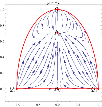
(a)

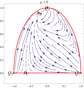
(b)

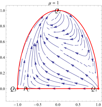
(c)

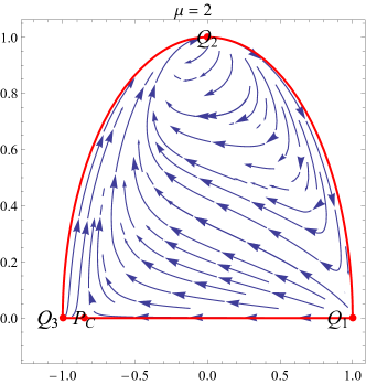
(d)

Figure 1: Orbits of the system (90) for some values of parameter $\mu$ in the Poincarè variables $(U,V)=\left(\frac{x}{\sqrt{1+x^{2}+z^{2}}},\frac{z}{\sqrt{1+x^{2}+z^{2}}}\right)$. The point $P_{B}$, whenever it exists, it is a sink. Point $P_{C}$ is always a saddle. The system admits three configurations at infinity $Q_{1}:(U,V)=(1,0)$, $Q_{2}:(U,V)=(0,1)$, and $Q_{3}:(U,V)=(-1,0)$, whose dynamics is shown in the plots.

It is worth noticing that the system (90) is integrable with general solution

$$x(\tau)=c_{1}e^{-3\tau}-\frac{\mu+2}{\sqrt{6}},\quad\Sigma_{+}(\tau)=c_{2}e^{-3\tau},\quad z(\tau)=\frac{6}{2\sqrt{6}c_{1}(\mu+2)e^{-3\tau}+6c_{3}e^{-6\tau}-\mu^{2}-4\mu+2}.$$ (91)

The equilibrium points are

$$P_{B}:(x,\Sigma_{+},z)=\left(-\frac{\mu+2}{\sqrt{6}},0,-\frac{6}{\mu(\mu+4)-2}\right),\quad P_{C}:(x,\Sigma_{+},z)=\left(-\frac{\mu+2}{\sqrt{6}},0,0\right).$$ (92)

The eigenvalues of $P_{B}$ are $\{-6,-3,-3\}$, therefore, it is a sink. On the other hand, $P_{C}$ has eigenvalues $\{6,-3,-3\}$, and it is a saddle. Interestingly, the equation for $\Sigma_{+}$ decouples, and we can study a reduced dynamical system for the variables $(x,z)$.

In Figures 1 are presented some orbits of system (90) for some values of parameter $\mu$ in the Poincarè variables $(U,V)$. The point $P_{B}$, whenever it exists, it is a sink. Point $P_{C}$ is always a saddle. The system admits three configurations at infinity $Q_{1}:(U,V)=(1,0)$, $Q_{2}:(U,V)=(0,1)$, and $Q_{3}:(U,V)=(-1,0)$, whose dynamics is shown in the plots. In this coordinates the set $P_{A}:(x,y,\Sigma_{+})=\left(x_{A},0,\Sigma_{+A}\right)$ is translated to $Q_{2}$ due to $\lim_{y\rightarrow 0}z=\infty,\lim_{z\rightarrow\infty}(U,V)=(0,1)$.

VI Conclusions

In this paper we have investigated a Lorentz violating Einstein-aether theory which contains a scalar field nonminimally coupled with the aether field. For the physical space we consider the homogeneous but anisotropic Bianchi I spacetime.

We have extended previous analyses on the subject by considering an interacting function between the scalar and the aether fields, which is nonlinear on the kinematic quantities of the time-like aether field. In particular we assume that the interacting function is quadratic on the expansion rate $\theta$ and on the shear $\sigma$, while in the generic scenario has three unknown functions of the scalar field, as expressed by equation (11).

The novelty of the interacting function under consideration is that we can determine a point-like Lagrangian and write the field equations by using the minisuperspace description. Indeed, the field equations can be seen as the motion of a point-like particle in a four-dimensional Riemannian space wich coordinates the three scalars of the Bianchi I spacetime and the field $\phi$, under the action of a potential function. By using this property, we are able to apply methods from Analytic Mechanics and study the integrability properties of the field equations. We use Ansätze for conservation laws which are linear in the momentum, such that it is possible to specify the unknown functions of the field equations, which allows for exact or analytic solutions of the field equations by using closed-form functions. Hence, the field equations are Liouville integrable.

In order to study the dynamics and the evolution of the anisotropies, we determine the equilibrium points for the field equations. These points describe some specific physical solutions for the model of our consideration. We perform our analysis by using the Hubble-normalized variables, also by using an alternative dimensionless variables which lead to the evolution of anisotropies with local and with Poincarè variables. From the two sets of variables we conclude that the isotropic spatially flat FLRW spacetime is a future attractor for the physical space. However, anisotropic solutions of Kasner-like are allowed by the theory of our consideration. Additionally, we have used the Center Manifold theorem and the Normal forms calculations to analyze the stability of sets of nonhyperbolic equilibrium points. All these tools lead to system’s reductions: Center Manifold and alternative formulations reduce the system dimensionality; whereas Normal Forms allow to eliminate non-resonant terms by using a sequence of nearly identity nonlinear transformations, keeping at each step only the terms at perturbation level which are relevant in the dynamics.

Finally, it is worth mentioning that our work contributes to the subject of Lorentz violating theories with a matter source. From the results of our analysis, it follows that real anisotropic physical solutions exist in Einstein-aether scalar field theory, while the generic evolution of the dynamics to an isotropic state in large scales, it is supported by the theory.

- (1) E.W. Kolb and M.S. Turner, The early universe, Addison-Wesley, New York (1990)
- (2) A. Guth, Phys. Rev. D 23, 347 (1981)
- (3) C.W. Misner, The Isotropy of the universe, Ap. J. 151 (1968) 431
- (4) O. Hrycyna and M. Szydlowski, Dynamics of the Bianchi I model with non-minimally coupled scalar field near the singularity, AIP Conf.Proc. 1514 (2013) 191
- (5) E. Russel, C. Battal Kilinc and O.K Pashaev Bianch I Model: An Alternative Way to Model The Presentday Universe, arXiv:1312.3502v3
- (6) K. Migkas, G. Schellenberger, T.H. Reiprich, F. Pacaud, M.E. Ramos-Ceja and L. Lovisari, A&A 636, A15 (2020)
- (7) A. S. Kompaneets and A. S. Chernov, Zh. Eksp. Teor. Fiz. (J. Exptl. Theoret. Phys. (U.S.S.R.)) 47 (1964) 1939 [Sov. Phys. JETP 20, 1303 (1965)].
- (8) R. Kantowski and R. K. Sachs, J. Math. Phys. 7, 443 (1966).
- (9) A. B. Burd and J. D. Barrow, Nucl. Phys. B 308, 929 (1988).
- (10) J. Yearsley and J. D. Barrow, Class. Quant. Grav. 13, 2693 (1996).
- (11) K.C. Jacobs, Astrophys J. 153, 661 (1968)
- (12) C.B Collins and S.W. Hawking, Astroph. J. 180, 317 (1973)
- (13) J.D. Barrow, Mon. Not. R. astron. Soc. 175, 359 (1976)
- (14) J.D. Barrow and D.H. Sonoda, Phys. Reports, 139, 1 (1986)
- (15) U. Nilsson and C. Uggla, Class. Quant. Grav. 13, 1601 (1996)
- (16) C. Uggla and H. Zur-Muhlen, Class. Quant. Grav. 7 1365 (1990)
- (17) M. Goliath, U. S. Nilsson and C. Uggla, Class. Quant. Grav. 15, 167 (1998)
- (18) B. J. Carr, A. A. Coley, M. Goliath, U. S. Nilsson and C. Uggla, Class. Quant. Grav. 18, 303 (2001)
- (19) A. Coley and M. Goliath, Class. Quant. Grav. 17, 2557 (2000)
- (20) A. Coley and M. Goliath, Phys. Rev. D 62, 043526 (2000)
- (21) M. Heusler, Phys. Lett. B 253, 33 (1991)
- (22) J.M. Aguirregabiria, A. Feinstein and J. Ibanez, Phys. Rev. D 48, 4662 (1993)
- (23) T. Christodoulakis, Th. Grammenos, Ch. Helias and P.G. Kevrekidis, J. Math. Phys. 47, 042505 (2006)
- (24) M. Tsamparlis and A. Paliathanasis, Gen. Relat. Gravit. 43, 1861 (2011)
- (25) A.A. Coley, J. Ibanez and R.J. van den Hoogen, J. Math. Phys. 38, 5256 (1997)
- (26) J. Ibanez, R.J. van den Hoogen and A.A. Coley, Phys. Rev. D 51, 928 (1995)
- (27) V.A. Belinskii, E.M. Lifhitz and I.M. Khalatnikov, JETP 33, 1061 (1971)
- (28) K. Adhav, A. Nimkar, R. Holey, Int. J. Theor. Phys. 46, 2396 (2007)
- (29) S.M.M. Rasouli, M. Farhoudi and H.R. Sepangi, Class. Quantum Grav. 28, 155004 (2011)
- (30) X.O. Camanho, N. Dadhich and A. Molina, Class. Quantum Grav. 32, 175016 (2015)
- (31) P. Halpern, Phys. Rev. D 63, 024009 (2001)
- (32) J.D. Barrow and T. Clifton, Class Quantum Grav. 23, L1 (2006)
- (33) T. Clifton and J.D. Barrow, Class Quantum Grav. 23, 2951 (2006)
- (34) A. Paliathanasis, J.D. Barrow and P.G.L. Leach, Phys. Rev. D 94, 023525 (2016)
- (35) A. Paliathanasis, J. Levi Said and J.D. Barrow, Phys. Rev. D 97, 044008 (2018)
- (36) T. Jacobson and D. Mattingly, Phys. Rev. D 64, 024028 (2001)
- (37) T. G. Zlosnik, P. G. Ferreira and G. D. Starkman, Phys. Rev. D 75, 044017 (2007)
- (38) I. Carruthers and T. Jacobson, Phys. Rev. D 83, 024034 (2011)
- (39) T. Jacobson, Phys. Rev. D 81, 101502 (2010) Erratum: [Phys. Rev. D 82 (2010) 129901]
- (40) T. Jacobson, PoS QG -PH, 020 (2007)
- (41) S. M. Carroll and E. A. Lim, Phys. Rev. D 70, 123525 (2004)
- (42) D. Garfinkle and T. Jacobson, Phys. Rev. Lett. 107 (2011) 191102
- (43) M. Roumeliotis, A. Paliathanasis, P.A. Terzis and T. Christodoulakis, EPJC 79, 349 (2019)
- (44) M. Roumeliotis, A. Paliathanasis, P.A. Terzis and T. Christodoulakis, EPJC 80, 239 (2019)
- (45) R. Chan, M.F.A. da Silva and V.H. Satheeshkumar, The General Spherically Symmetric Static Solutions in the Einstein-Aether Theory, [arXiv:2003.00227]
- (46) C. Ding, C. Liu, R. Casana and A. Cavalcante, EPJC 80, 178 (2020)
- (47) D. Vernieri, Phys. Rev. D 100, 104021 (2019)
- (48) A. A. Coley, G. Leon, P. Sandin and J. Latta, JCAP 1512, 010 (2015)
- (49) J. Bhattacharyya, A. Coates, M. Colombo and T.P. Sotiriou, Phys. Rev. D 93, 064056 (2016)
- (50) M. Gürses, Gen. Relativ. Gravit. 41, 31 (2009)
- (51) M. Gürses and C. Sentürk, Gen. Relativ. Gravit. 48, 63 (2016)
- (52) A. Paliathanasis, doi.org/10.1088/1361-6382/ab8145
- (53) C. Ranjit, P. Rudraand S. Kundu, EPJP 129, 208 (2014)
- (54) A.B. Balakin and J.P.S. Lemos, Annals Phys. 350, 454 (2014)
- (55) W. Doneely and T. Jacobson, Phys. Rev. D 82, 064032 (2010)
- (56) S. Kanno and J. Soda, Phys. Rev. D 74, 063505 (2006)
- (57) B. Alhulaimi, R.J. van den Hoogen and A.A. Coley, JCAP 17, 045 (2017)
- (58) R.J. van de Hoogen, A.A. Coley, B. Alhulaimi, S. Mohandas, E. Knighton and S. O’Neil, JCAP 18, 017 (2018)
- (59) J. Latta, G. Leon and A. Paliathanasis, JCAP 1611, 051 (2016)
- (60) A. Coley and G. Leon, Gen. Rel. Grav. 51, no. 9, 115 (2019)
- (61) G. Leon, A. Coley and A. Paliathanasis, Annals Phys. 412, 168002 (2020)
- (62) P. Sandin, B. Alhulaimi and A. Coley, Phys. Rev. D 87, 044031 (2013)
- (63) A. Paliathanasis, G. Papagiannopoulos, S. Basilakos and J.D. Barrow, EPJC 79, 723 (2019)
- (64) A. Paliathanasis, Phys. Rev. D 101, 064008 (2020)
- (65) J.D. Barrow, Phys. Rev. D 85, 047503 (2012)
- (66) A.R. Solomon and J.D. Barrow, Phys. Rev. D 89, 024001 (2014)
- (67) A. Paliathanasis and G. Leon, Analytic solutions in Einstein-aether scalar field cosmology, to appear in EPJC (2020) [arXiv:2003.03903]
- (68) V. G. LeBlanc, D. Kerr and J. Wainwright, Class. Quant. Grav. 12, 513 (1995) cited in reza .
- (69) Arrowsmith D. K. and Place C. M., 1990, “An introduction to Dynamical Systems”, Cambridge University Press.
- (70) Wiggins S., 1990, “Introduction to Applied Nonlinear Dynamical Systems and Chaos”, Springer-Verlag, New York; Wiggins S., 2003, “Introduction to Applied Nonlinear Dynamical Systems and Chaos”, Springer.
- (71) R. Tavakol, “Introduction to dynamical systems,” ch. 4, Part one, pp. 84–98, Cambridge University Press, Cambridge, England, 1997.
- (72) Aulbach B., 1984, “Continuous and Discrete Dynamics near Manifolds of Equilibria”, Lecture Notes in Mathematics, N0. 1058, Springer-Verlag, cited in “Dynamical Systems in Cosmology”, edited by Wainwright J. and Ellis G.F.R. (Cambridge University Press, Cambridge).
- (73) Carr J., 1981, “Applications of Center Manifold Theory”, Springer-Verlag, cited in “Dynamical Systems in Cosmology”, edited by Wainwright J. and Ellis G.F.R. (Cambridge University Press, Cambridge).
- (74) Arnold V I 1988 Geometrical Methods in the Theory of Differential Equations (Berlin: Springer)
- (75) Arnold V I and Il’yashenko Yu S 1988 Ordinary differential equations Dynamical systems, Encyclopaedia of Mathematical Sciences vol I, ed D V Anosov and V I Arnold (Berlin: Springer) pp 1–148
- (76) Bruno A D 1989 Local Methods in Nonlinear Differential Equations (Berlin: Springer)
- (77) Verhulst F 1990 Nonlinear Differential Equations and Dynamical Systems (Berlin: Springer)
- (78) Verhulst F 1996 Nonlinear Differential Equations and Dynamical Systems 2nd edn (Berlin: Springer)
- (79) S. Basilakos, M. Tsamparlis and A. Paliathanasis, Phys. Rev. D 83, 103512 (2011)
- (80) A. Paliathanasis, M. Tsamparlis and S. Basilakos, Phys. Rev. D 84, 123514 (2011)
- (81) M. Tsamparlis and A. Paliathanasis, Symmetry 10, 233 (2018)
- (82) M. Crampin, Reports Math. Phys. 20, 31 (1984)
- (83) M. Cariglia, Rev. Mod. Phys. 86, 1283 (2014)
- (84) L. Karpathopoulos, M. Tsamparlis and A. Paliathanasis, J. Geom. Phys. 133, 279 (2018)
- (85) A. Paliathanasis and P.G.L. Leach, J. Math. Phys. 57, 024101 (2016)
- (86) L. Amendola, D. Polarski and S. Tsujikawa, IJMPD 16, 1555 (2007)
- (87) G. Leon and E.N. Saridakis, JCAP 1504, 031 (2015)
- (88) G. Leon, IJMPE 20, 19 (2011)
- (89) T. Gonzales, G. Leon and I. Quiros, Class. Quantum Grav. 23, 3165 (2006)
- (90) A. Giacomini, S. Jamal, G. Leon, A. Paliathanasis and J. Saveedra, Phys. Rev. D 95, 124060 (2017)
- (91) G. Papagiannopoulos, P. Tsiapi, S. Basilakos and A. Paliathanasis, EPJC 80, 55 (2020)
- (92) S. Mishra and S. Chakraborty, EPJC 79, 328 (2019)
- (93) G. Leon and A. Paliathanasis, EPJC 79, 746 (2019)
- (94) D. Escobar, C.R. Fadragas, G. Leon and Y. Leyva, Class. Quantum Grav. 29, 175006 (2012)
- (95) M. Cruz, A. Ganguly, R. Gannouji, G. Leon and E.N. Saridakis, Class. Quantum Grav. 34, 125014 (2017)
- (96) E.J. Copeland, M. Sami and S. Tsujikawa, IJMPD 15, 1753 (2006)