Indoor Millimeter-Wave Systems: Design and Performance Evaluation

Abstract

Indoor areas, such as offices and shopping malls, are a natural environment for initial mmWave (mmWave) deployments. While we already have the technology that enables us to realize indoor mmWave deployments, there are many remaining challenges associated with system-level design and planning for such. The objective of this article is to bring together multiple strands of research to provide a comprehensive and integrated framework for the design and performance evaluation of indoor mmWave systems. The paper introduces the framework with a status update on mmWave technology, including ongoing 5G wireless standardization efforts, and then moves on to experimentally-validated channel models that inform performance evaluation and deployment planning. Together these yield insights on indoor mmWave deployment strategies and system configurations, from feasible deployment densities to beam management strategies and necessary capacity extensions.

I Introduction

Our motivation in this article is to present a comprehensive framework for performance evaluation and design practices dedicated to indoor mmWave (mmWave) networks. The framework integrates inputs from multiple areas of mmWave networking expertise, from standardization, to channel measurements and modelling, to system-level evaluations and deployment planning. Its major contribution is insights into indoor mmWave deployment planning strategies and system configurations that are grounded and informed by experimentally-validated channel models.

mmWave are a natural choice for mobile indoor deployments due to much shorter link distances, weak penetration through walls, and large available bandwidths. In fact, the concept of using mmWave to provision multi-Gbps speeds over indoor areas dates back to works published in the late 90’s [1, 2]. Later came a suite of standards that offered the possibility of ad hoc networking, including ECMA-387 [3], IEEE 802.15.3c [4], and more recently IEEE Wireless Gigabit 802.11ad/ay [5, 6]. Nowadays, the importance of mmWave keeps increasing, since they are one of the key mobile broadband networking features of the 5G (5G) wireless [7], [8].

At the time of writing, the first set of 5G-NR specifications had already been defined as part of the 3GPP (3GPP) Release 15, functionally frozen in September 2018. Work on Release 16 is ongoing and is planned to be frozen in June 2020, with Release 17 to follow. The FR (FR) considered for deploying mmWave technology, as agreed in Release 15, is from 24.25 GHz to 52.6 GHz, also referred to as FR2. FR2 currently addresses three bands: 24.25–27.5 GHz (n257), 26.5–29.5 GHz (n258), and 37–40 GHz (n260), all meant to support TDD (TDD) operation only. Usage of frequencies between 52.6 GHz and 71 GHz is currently under study in Release 17. In particular, the spectrum around 60 GHz presents an attractive use case, as it: a) does not require licenses, and b) is harmonised globally [9]. In this spectrum, the 3GPP is planning to deploy NR-based access technology – NR-U (NR-U) – which will incorporate extensions necessary to work in unlicensed spectrum. NR-U will account for national restrictions of the 60 GHz band, which the 3GPP had already identified in Release 14 [10]. In Fig. 1, we summarize the adoption of mmWave spectrum for 5G-NR.

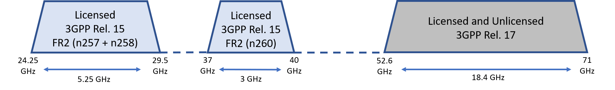
Figure 1: Status of the mmWave spectrum for 5G-NR.

As part of its 5G activity, the 3GPP defined the eMBB (eMBB) Indoor Hotspot scenario as a natural case study for indoor mmWave mobile networks [11]. The key purpose of this scenario is to provision small-cell coverage of high data rates and capacity to a user population within a confined area. Typical examples for this type of scenario include an open office, airport hall, or shopping mall. For such a setup, one would be interested in understanding the required density of access points, deployment locations, and effective network settings. Understanding these system design aspects requires adequate system-level evaluation that involves similarly adequate representation of the mmWave channel.

There are many ongoing measurement campaigns being conducted around the globe with the aim of characterizing and modeling the mmWave propagation channel, e.g., [12, 13, 14, 15, 16]. By their nature, all these measurements are context-specific (as any experimental work), and, depending on the modeling technique used, pertain to different types of system-level evaluations. For example, in an open office scenario, radio infrastructure is typically mounted to the ceiling or walls, illuminating the main area inside [17]. In such a setup, the main factor limiting signal propagation is shadowing by physical objects [18]. In particular, human bodies introduce extra attenuation, referred to as body blockage, which may vary with the orientation and position of the bodies with respect to both the device and the serving access point [19]. However, whether the communication link is blocked or not will also have a discernible effect on the fading characteristics of the associated wireless channel. Broadly speaking, blocked links often display a richer multipath structure, with weaker direct component and larger delay spread, than the unobstructed ones [14]. Moreover, it was found that within indoor locations, such as large offices and hallways, body-related blockage has a less pronounced effect on the received signal power, most likely due to the increased scattering in the environment [19]. The trick is to capture all of these propagation-related effects in a model that is both accurate and amenable to the analysis at system-level.

In what follows we describe our framework by first discussing our channel measurement campaign and a modelling approach that we subsequently integrate into both system-level evaluations and deployment planning. Using this framework, we provide insights on feasible deployment densities, beam management strategies, and necessary capacity extensions. While the framework can be applied to any indoor mmWave networking scenario, our case study focuses on an open office environment for illustrative purposes.

II Indoor mmWave channel

It is well known that many aspects of wireless communications, e.g., system design, network topology and performance, are dependent upon an accurate understanding of the channel characteristics. Therefore, channel characteristics at mmWave must be comprehensively studied to allow detailed channel models to be developed. This knowledge will both inform the design of future mmWave communications systems and help predict important performance measures such as the achievable coverage probabilities and capacities. In wireless communications channels, the characteristics of the received signal are often characterized in terms of path loss, shadowing and small-scale fading. In what follows, we introduce the $\kappa$-$\mu$ fading model and provide empirical evidence for its utility and versatility in the context of mmWave communications, in particular for indoor hotspot eMBB applications, which is one of the five test use cases selected in [17].

II-A Indoor mmWave Channel Measurements

A number of studies have recently been conducted in [20, 13, 5, 21, 22, 23, 24], which are key to the provisioning of future 5G services at mmWave frequencies for both indoor and outdoor environments. In most previous mmWave channel studies [22, 23, 24], the measurements have considered the case where both the TX (TX) and RX (RX) are stationary and mounted on stands. In some of these studies [22, 23], obstructions in the optical LOS path between the TX and RX are analyzed. Crucially, however, none of these studies considers scenarios where the TX and/or RX are in close proximity to the human user body. To this end, in this work, we have considered the case where a hypothetical UE (UE) (i.e., the TX in our case) is held by the user while emulating different UE operating modes. Furthermore, the user is moving through the environment. This is driven by the need to understand the potential impact of UE operation mode and user mobility on the small-scale fading characteristics, knowledge of which will be essential for determining the localized performance of future user-centric mmWave networks.

II-A1 Measurement System and Environments

To emulate a possible indoor hotspot eMBB use case the mmWave channel between a UE and AP (AP) is considered. The hypothetical UE and AP used for the mmWave channel measurements are shown in Fig. 2(a) and (b), respectively. Details of the hypothetical UE and AP can be found in [25]. The channel measurements were conducted within a hallway (17.38 m $\times$ 1.40 m) and an open office area (10.62 m $\times$ 12.23 m) as shown in Fig. 3. Both the hallway and open office environments are located on the 1^st floor of the Institute of Electronics, Communications and Information Technology (ECIT) at Queen’s University Belfast in the United Kingdom. Both environments featured metal studded dry walls with a metal tiled floor covered with polypropylene-fiber, rubber backed carpet tiles, and metal ceiling with mineral fiber tiles and recessed louvered luminaries suspended 2.70 m above floor level. The open office area contained a number of soft partitions, cabinets, personal computers, chairs and desks. It should be noted that both the hallway and open office environments were unoccupied for the duration of the channel measurements and the AP was placed above a ceiling tile with the antenna boresight oriented towards the floor, i.e., imitating a ceiling-mounted AP.

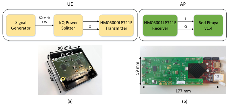
Figure 2: Hypothetical (a) UE and (b) AP used for the mmWave channel measurements.

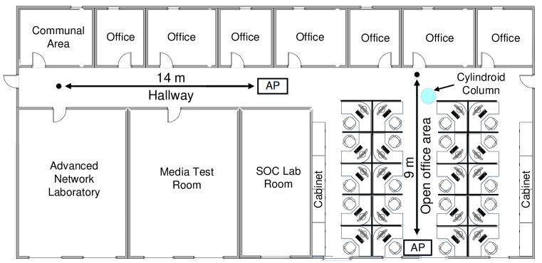
Figure 3: Indoor hallway and open office environments considered in this study along with annotated user trajectories.

II-A2 Usage Cases

During the measurements, the UE was operated by an adult male of 1.83 m in height and mass 80 kg. A number of different use cases likely to be encountered in everyday scenarios were considered. These were: (1) operating an app, where the user held the UE with his two hands in front of his body; (2) carrying a device I, where the UE was located in the right-front pocket of the user’s clothing; (3) carrying a device II, where the user held the UE with his right hand beside his right leg. Herein, and for brevity, we denote the three different UE usage cases as app, pocket and hand respectively. In this study, we considered two different dynamic channel conditions, namely, (1) mobile LOS and (2) mobile NLOS (NLOS), where the user walked towards and away from the hypothetical AP in a straight line, respectively. It is worth remarking that the NLOS channel conditions occurred when the direct optical path between the UE and AP was obstructed by the user’s body, i.e., self-blockage.

To improve the validity and robustness of the parameter estimates obtained in this study, all the measurements were repeated three times. Due to the dissimilar sizes of each environment, the considered walking distances were different. In particular, these were 9 m and 14 m for the open office area and hallway respectively. The average walking speed maintained by the user throughout all of the experiments was approximately 1 m/s.

II-A3 Path Loss

The path loss is a measure of the signal attenuation between the transmitter and receiver as a function of the separation distance and can be expressed as [26]

$$P\left[{\rm dB}\right]=P_{0}\left[{\rm dB}\right]+10\alpha\log_{10}\left({d}/{d_{0}}\right),$$ (1)

where $P_{0}$ represents the path loss at the reference distance $d_{0}$, $\alpha$ is the path loss exponent which indicates the rate at which the path loss increases with distance and $d$ is the separation distance between the transmitter and receiver. To obtain estimates for $P_{0}$ and $\alpha$, we first removed the EIRP (EIRP) and gain at the receiver from the raw signal power received by the AP and then performed linear regression. To enable this, the elapsed time was first converted into a distance using the test user’s velocity. The reference distance, which should be in far field region of the antenna, was chosen to be 1 m for all environments. The mean values of the parameter estimates for $P_{0}$ and $\alpha$ averaged over all the trials for all of the considered cases are given in Table I along with the body blockage, which is defined as the difference between the path loss at the reference distance (i.e., $P_{0}$) for the LOS and NLOS conditions. The path loss exponents for the LOS scenarios were found to be smaller than that associated with isotropic radiation in free space ($\alpha=2$). This was possibly due to the waveguide effect which can often be present within indoor environments [28]. As anticipated, for both the hallway and office environments, the $P_{0}$ values for the NLOS were greater than those for the LOS due to the shadowing effects caused by the test user’s body. When considering the values of the body blockage, it was observed that the hand case had a smaller body blockage compared to those for the app and pocket cases. This confirms the intuition that the UE to ceiling-mounted AP channel is less susceptible to body blockage when the user is carrying the UE further away from the body, which is the case with the hand scenario.

II-A4 Small-Scale Fading

The $\kappa$-$\mu$ distribution has been proposed as a generalized statistical model, which may be used to characterize the random variation of the received signal caused by multipath fading [29]. The PDF (PDF) of the signal envelope, $H$, in a $\kappa$-$\mu$ fading channel can be expressed as

$$f_{{H}}({h})=\frac{{2\mu{{\left({\kappa+1}\right)}^{\frac{{\mu+1}}{2}}}{h}^{\mu}}}{{{\kappa^{\frac{{\mu-1}}{2}}}\exp\left({\mu\kappa}\right){\Omega^{\frac{{\mu+1}}{2}}}}}\exp\left({\frac{{-\mu\left({\kappa+1}\right){h}^{2}}}{\Omega}}\right){I_{\mu-1}}\left({2\mu\sqrt{\kappa\left({\kappa+1}\right)}\frac{{{h}}}{{\sqrt{\Omega}}}}\right),$$ (2)

where $I_{v}(\cdot)$ represents the modified Bessel function of the first kind with order $v$. In terms of its physical interpretation, $\kappa$ is defined as the ratio between the total power in the dominant signal components and the total power in the scattered signal components, $\mu$ is the number of multipath clusters and $\Omega$ is the mean signal power given by $\Omega=\mathbb{E}[H^{2}]$.

TABLE I: Average Parameter Estimates for the Path Loss Model and $\kappa$-$\mu$ Fading Model for All of the Cases

Environ-	Use Case	LOS					NLOS					Body
ment		$\bar{\alpha}$	$\bar{P_{0}}{\rm[dB]}$	$\bar{\kappa}$	$\bar{\mu}$	$\bar{\Omega}$	$\bar{\alpha}$	$\bar{P_{0}}{\rm[dB]}$	$\bar{\kappa}$	$\bar{\mu}$	$\bar{\Omega}$	Blockage
Hallway	app	1.92	78.31	2.80	0.77	1.16	1.93	95.39	0.67	0.96	1.25	17.09 dB
	pocket	1.92	82.55	2.64	0.78	1.17	1.95	95.60	0.47	1.02	1.24	13.05 dB
	hand	1.93	90.42	1.89	0.88	1.18	1.94	97.49	0.89	0.99	1.22	7.06 dB
Office	app	2.58	81.31	1.14	1.00	1.21	1.03	101.41	0.48	1.00	1.26	20.09 dB
	pocket	1.38	92.32	1.46	0.91	1.21	1.01	102.11	0.46	1.00	1.26	9.79 dB
	hand	1.52	95.74	1.24	0.93	1.21	1.38	101.83	0.50	1.04	1.24	6.09 dB

The small-scale fading was extracted by removing both the path loss and large-scale fading from the channel data before transforming the data to its linear amplitude. The parameter estimates for the $\kappa$-$\mu$ fading model were obtained using a non-linear least squares routine. Table I provides the mean parameter estimates for the $\kappa$-$\mu$ fading model averaged over all three trials for each of the UE to AP channels.

Our first observation is that the obtained results provide evidence for the correctness of our methodology. For all of the LOS scenarios and environments, the $\kappa$ parameters were found to be greater than unity ($\kappa>1$), indicating the presence of a strong dominant signal component. In contrast, for the NLOS scenarios (i.e., when the direct signal path was blocked by user’s body), the $\kappa$ parameters were smaller than unity ($\kappa<1$), indicating the absence of a dominant signal contribution. Additionally, for the NLOS scenarios, the $\kappa$ parameters obtained for the hand case were slightly greater than those for the app and pocket cases, suggesting that the UE to ceiling-mounted AP link for the hand is less impacted by the human body blockage. The $\mu$ parameters for the LOS scenarios were slightly smaller than those obtained for the NLOS scenarios. This suggests that the signal fluctuation observed in the LOS scenarios is less impacted by multipath clustering compared to that experienced in NLOS. As an example of the fits obtained, Fig. 4 presents the empirical PDF of the small-scale fading alongside the $\kappa$-$\mu$ PDF for all of the UE usage cases while the operator walked towards the hypothetical AP in the hallway environment. It is clear that the $\kappa$-$\mu$ fading model is in excellent agreement with the measurement data.

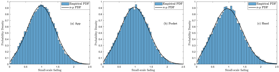
Figure 4: Empirical (bars) and theoretical (continuous lines) PDF of the small-scale fading observed in the hallway environment for the LOS scenario with (a) app, (b) pocket and (c) hand cases.

To ascertain the most probable model between the $\kappa$-$\mu$ and Rayleigh distributions for characterizing the small-scale fading observed in the UE-to-AP channels, the AIC was employed. More specifically, the AICc (AICc) was used in a similar manner to the analysis employed in [30], such that

$$\mathrm{AIC}_{c}=-2\ln\left({l\left({\theta|\text{data}}\right)}\right)+2M+\frac{{2M\left({M+1}\right)}}{{n-M-1}}$$ (3)

where $\ln\left({l\left({\theta|\text{data}}\right)}\right)$ is the value of the maximized log-likelihood for the unknown parameter $\theta$ of the model given the data, $M$ is the number of estimated parameters available in the model, and $n$ is the sample size. It should be noted that the lower the AICc value, the more likely the candidate model was to have generated the data. As shown in Table II, the $\kappa$-$\mu$ and Rayleigh fading models were ranked according to their AICc. It is clear that the $\kappa$-$\mu$ distribution was selected as the best model for all of the considered cases, suggesting that the added complexity (i.e., additional parameters) in the $\kappa$-$\mu$ model is worthwhile.

TABLE II: $AIC_{c}$ rank for all of the considered UE-to-AP channel measurement data.

Environment	Use Case	LOS		NLOS
		$\kappa$-$\mu$	Rayleigh	$\kappa$-$\mu$	Rayleigh
Hallway	app	1	2	1	2
	pocket	1	2	1	2
	hand	1	2	1	2
Office	app	1	2	1	2
	pocket	1	2	1	2
	hand	1	2	1	2

III System-Level Modelling and Performance Evaluation

Indoor mmWave networks will be characterised by much shorter distances between access points and users as well as deployments that will be confined to closed areas and made independent from outdoor deployments due to weak out-in penetration [31]. In Section II, we also reported that in the presence of a human user body the indoor mmWave channel becomes highly complex with a mix of large- and small-scale fading effects. Understanding how the basic network parameters such as access point density, antenna beamwidth, and serving distance will impact network performance in these conditions requires new and extensive system-level modelling approaches.

In this section we develop an analytical framework and quantify the performance of indoor mmWave networks. Our framework bridges the statistical channel models obtained from measurement campaigns, described in Section II, with stochastic network geometry, which reflects the fact that at any given point in time the set of user locations and/or transmitter directionalities may be considered random. Our framework yields analytical expressions describing the distribution of the SINR (SINR) in a generic indoor mmWave network. While the obtained expressions are too complex to be amenable to intuition, they allow us to generate numerical results that we can use to cross-validate corresponding Monte Carlo simulations. Ultimately, we use both the analytical expressions and simulations to explore the relationship between basic network parameters, channel scenarios and network performance indicators: coverage, ATC (ATC), and EDR (EDR), which we define in Section III-B.

Most work to date on system-level evaluations for mmWave networking are focused on large-scale outdoor areas, e.g., [32, 33, 34]. Indoor area mmWave network analysis has received much less attention, with some earlier works considering device-to-device applications [35, 36], and more recent works addressing hotspot deployments [37, 38, 39, 40]. While building on the relevant literature, our work presented in this section goes beyond it in two important ways. First, expanding on our work in [41], we offer analysis based on the experimentally-validated $\kappa$-$\mu$ fading model, which allows us to consider the impact that different device usage scenarios have on network performance. Then, the network setup we consider is aligned with network setups recommended for system-level evaluation of mobile mmWave systems [42, 11]. For these we provide analytical expressions describing network performance which, for special cases, can be reduced to closed-form expressions.

III-A System Model

Network Geometry

We consider a network with $n_{\mathrm{TX}}$ transmitters $\Phi=\{x_{0},x_{1},\ldots,x_{n_{\mathrm{TX}}-1}\}\subset\mathcal{W}$, whose locations are uniformly distributed over a finite arbitrary area $\mathcal{W}\subset\mathbb{R}^{2}$. Our analysis takes the perspective of the reference receiver, which is an arbitrary point in $\mathcal{W}$ at distance $\rho_{0}$ from the center of mass of $\mathcal{W}$. Since we are interested in analyzing feasible networks, we consider $\mathcal{W}$ to always contain the reference receiver and the transmitter serving that reference receiver (the serving transmitter), which, in our notation, is always indexed as 0. On the horizontal plane, the reference receiver and the serving transmitter are a distance $r_{0}\geq 0$ apart. We will refer to the wireless link between the reference receiver and its transmitter as the reference link. Transmissions from remaining $n_{\mathrm{TX}}^{\prime}=n_{\mathrm{TX}}-1$ transmitters will be treated as interference to the reference link. We assume that all transmitters are located at height $h_{\mathrm{TX}}$ above the ground, with the reference receiver operating at height $h_{\mathrm{RX}}$.

Directionality Gain

All transmitters and receivers utilize directional transmission and reception. We assume the transmitter (receiver) antenna gain is calculated based on the cone-bulb model [37]. In this model the main-lobe gain $\text{G}_{\mathrm{TX}}$ is a function of the beamwidth $\omega_{\mathrm{TX}}$, normalized over the whole spherical surface:

$$\text{G}_{\mathrm{TX}}\frac{1-\cos(\omega_{\mathrm{TX}}/2)}{2}-\text{g}_{\mathrm{TX}}\frac{1+\cos(\omega_{\mathrm{TX}}/2)}{2}=1,$$ (4)

where $\text{g}_{\mathrm{TX}}$ is the side-lobe gain. Correspondingly, we will use $\text{G}_{\mathrm{RX}}$, $\text{g}_{\mathrm{RX}}$, and $\omega_{\mathrm{RX}}$ to refer to the main-lobe gain, side-lobe gain, and beamwidth of the receiver antenna. Usage of the cone-bulb model and the main-lobe beamwidth as our parameter abstracts our analysis from the choice of the antenna system, and makes our results applicable to scenarios with fixed directional antennas. This could be the case, for example, in lecture halls or open offices where users remain static. Conversion between beamwidth, antenna gain, and number of antenna elements for various types of antennas can be found in [43]. Let us note that the cone-bulb model is also a risk-averse choice as it leads to underestimation of coverage results [44].

Then the directionality gain is the product of transmitter and receiver antenna gains, which depend on the beam alignment between the two [45]. Using the convention that the alignment gain between the receiver and a transmitter is random, we can represent it as a four-dimensional categorical random variable $G_{i}$, with $i\in\{0,\ldots,n_{\mathrm{TX}}-1\}$. This random variable maps from the space of all possible alignments between the transmitter $i$ and the reference receiver to the space of alignment gains $\mathcal{G}$ that is formed as a product of the transmitter and receiver antenna gains, with the corresponding probability mass function $p_{g_{i}}=\mathbb{P}(G_{i}=g_{i})$. In practice the alignment gain from the serving transmitter is maintained stable by beam management operations, which corresponds to conditioning $G_{0}=g_{0}$, where $G_{0}$ is the alignment gain on the reference link and $g_{0}$ a constant.

Blockage

In our framework, link blockage arises from self-blockage, i.e., blockage of the LOS signal path between the receiver and the transmitter by the human user. The severity of this blockage will depend on the usage scenarios defined in Section II: app with a device held in front of the user, pocket with a device held in the front pocket, hand with a device carried in the hand. For each scenario, we consider fixed blockage on the reference link and probabilistic blockage on all other links. Consequently, blockage is a Bernoulli random variable, with the success probability $p_{\mathrm{LOS}}$ and $p_{\mathrm{NLOS}}=1-p_{\mathrm{LOS}}$, where the latter is referred to as the blockage probability. Here we opt for a model where $p_{\mathrm{LOS}}$ (or, indeed, $p_{\mathrm{NLOS}}$) is simply a system parameter that reflects the frequency of link blockages. Furthermore, we assume that each transmission link experiences blockages independently of all other links. Numerical evaluations in [40] show that this independence assumption results in negligible differences to the blockage probability.

Propagation Model

We use the model as proposed in Section II, but to capture the bifurcation of its parameters (due to link blockage) we adopt the following notation for the path loss and power fading:

$$l_{t}(r_{i})=\gamma_{t}r_{i}^{\alpha_{t}},\qquad f_{H_{i,t}}(h)=\frac{\theta_{1,t}^{(\mu_{t}+1)/2}}{\theta_{2,t}^{(\mu_{t}-1)/2}}h^{(\mu_{t}-1)/2}\exp\left(-\theta_{1,t}h-\theta_{2,t}\right)I_{\mu_{t}-1}\left(2\sqrt{\theta_{1,t}\theta_{2,t}h}\right),$$ (5)

where $r_{i}$, with $i\in\{0,\ldots,n_{\mathrm{TX}}-1\}$, is the distance to the $i$-th transmitter, $t\in\{\mathrm{LOS},\mathrm{NLOS}\}$ blockage state, $\gamma_{i,t}$ path loss at the reference distance (in linear scale), $\alpha_{t}$ path loss exponent, $\theta_{1,t}=\frac{\mu_{t}(1+\kappa_{t})}{\sqrt{\Omega_{t}}}$, and $\theta_{2,t}=\mu_{t}\kappa_{t}$. Scattering and diffraction via static objects, such as inner walls or office furniture, are not explicitly modelled, yet their impact is included in the parameter values given in Table I.

Signal-to-Interference-and-Noise Ratio

Given a transmitter at $x_{i}$ and blockage state $t\in\{\mathrm{LOS},\mathrm{NLOS}\}$, the instantaneous power received at the reference receiver located in $y_{0}\in\mathcal{W}$ is:

$$S_{i,t}=G_{i}H_{i,t}l_{t}\left(r_{i}\right),$$ (6)

where $r_{i}=\sqrt{||x_{i}-y_{0}||^{2}+(h_{\mathrm{TX}}-h_{\mathrm{RX}})^{2}}$ is the distance between the reference receiver and transmitter $i$, $H_{i,t}$ is the blockage-dependent power fading, and $l_{t}\left(r_{i}\right)$ is the blockage-dependent path attenuation. Then the SINR, under blockage state $t$ on the serving channel is given by

$$\mathrm{SINR}=\frac{S_{0,t}}{I+\tau^{-1}},$$ (7)

where $S_{0,t}$ is the instantaneous power received from the serving transmitter, $I=\sum_{i=1}^{n_{\mathrm{TX}}^{\prime}}S_{i}$ is the interference power, with $S_{i}=\mathbb{E}_{V_{i}}[S_{i,V_{i}}]$ being the received signal power from transmitter $i$ averaged over random blockage states $V_{i}\in\{\mathrm{LOS},\mathrm{NLOS}\}$ on link $i$, and $\tau$ is the signal-noise ratio.

III-B Network Performance Characterization

We utilize three key performance indicators recommended by the 3GPP [11]: coverage, ATC, and EDR. Broadly speaking, the first represents the coverage achievable in our network, the second provides us with information on the expected user throughput, and the third represents the throughput achievable by a subset of users with the worst channel.

Coverage

We represent the coverage as the probability that the SINR is greater than some pre-defined coverage threshold $\zeta$, which is equivalent to finding the CCDF (CCDF) of the SINR:

$$\mathbb{P}(\mathrm{SINR}>\zeta)=F^{c}_{\mathrm{SINR}}(\zeta).$$ (8)

Area traffic capacity

ATC is a measure of the total traffic a network can serve per unit area (in $\text{bit/s/m}^{2}$), which can be calculated as:

$$C_{\mathrm{area}}=\lambda\times\mathrm{bw}\times\mathrm{SE},$$ (9)

where $\lambda$ is the transmitter density, $\mathrm{bw}$ is the transmission bandwidth, and $\mathrm{SE}$ is the spectral efficiency. The spectral efficiency is the average data rate per unit of spectrum and per cell, which can be expressed in terms of the CCDF of the SINR as:

$$\mathrm{SE}=\int_{0}^{\infty}\mathbb{P}\left(\log(1+\mathrm{SINR})>r\right)\differential{r}=\int_{0}^{\infty}\mathrm{F}^{c}_{\mathrm{SINR}}\left(2^{r}-1\right)\differential{r}.$$ (10)

Experienced data rate

We define the EDR as the 5^th percentile of the user throughput distribution, which can also be found numerically following the approach proposed in [46]:

$$q_{R}(\beta=0.05)=\operatorname*{\arg\!\min}_{u}\Big{\{}u+\frac{1}{1-\beta}\int_{u}^{\infty}\mathrm{F}^{c}_{\mathrm{SINR}}\left(2^{r/\mathrm{bw}}-1\right)\differential{r}\Big{\}}.$$ (11)

III-C Analytical Results

In the following we provide our main analytical results. We start with the distribution of the received power in Lemma 1, which we subsequently use to characterize the CCDF of the SINR for a mmWave network distributed over an arbitrary finite area in Lemma 2. Finally, we specialize this result to the case of a network distributed over a disk in Corollary 1.

Lemma 1 (Received Power Statistics)

Given transmitter $i$ at distance $r_{i}$, directionality gain $g_{i}$, and blockage state $t$, the CCDF of $S_{i,t}$ can be expressed as:

$$\begin{split}\mathbb{P}\left(S_{i,t}>x\right)&=\exp(-\theta_{2,t})\sum_{l=0}^{\infty}\frac{\theta_{2,t}^{l}}{l!}\sum_{n=0}^{l+\mu_{t}-1}\frac{1}{n!}\left(\frac{\theta_{1,t}x}{\vartheta_{i,t}}\right)^{n}\exp\left(-\frac{\theta_{1,t}}{\vartheta_{i,t}}x\right),\end{split}$$ (12)

where $\theta_{1,t}$ and $\vartheta_{i,t}$ are provided in (5) and (29), respectively.

Proof:

The above formula relies on a simple re-formulation of the PDF in (5), and the subsequent calculation of the resulting CDF (CDF), which is presented in Appendix A. ∎

Remark 1 (Other representation of Lemma 1)

In Lemma 1 we define the received power distribution using infinite series representation to facilitate further derivations of the SINR. However, the distribution in question can also be represented in closed-form, as shown in [29], utilizing the generalized Marcum-Q function.

Lemma 2 (Distribution of SINR for an Arbitrary Area)

Given the distance to the serving transmitter $r_{0}$, its directionality gain $g_{0}$ and LOS blockage state $t$, the conditional CCDF of the SINR is given by

$$\begin{split}&\mathbb{P}\left(\mathrm{SINR}>\zeta\big{|}G_{0}=g_{0},R_{0}=r_{0},T_{0}=t\right)=\\ &\exp\left(-\theta_{2,t}-\frac{\zeta\theta_{1,t}}{\vartheta_{0,t}\tau}\right)\sum_{l=0}^{\infty}\frac{\theta_{2,t}^{l}}{l!}\sum_{n=0}^{l+\mu_{t}-1}\frac{1}{n!}\left(\frac{\zeta\theta_{1,t}}{\vartheta_{0,t}\tau}\right)^{n}\sum_{k=0}^{n}{n\choose k}\tau^{k}\\ &\sum_{k_{1}+k_{2}+\ldots+k_{n_{\mathrm{TX}}^{\prime}}=k}{k\choose k_{1},k_{2},\ldots,k_{n_{\mathrm{TX}}^{\prime}}}\prod_{1\leq i\leq n_{\mathrm{TX}}^{\prime}}\sum_{v\in\{\mathrm{LOS},\mathrm{NLOS}\}}p_{v}\sum_{g\in\mathcal{G}}p_{g}(\mu_{v})_{k_{i}}\theta_{1,v}^{\mu_{v}}g^{k_{i}}\exp(-\theta_{2,v})\mathfrak{Z}_{k_{i}},\\ &\text{where}\quad\mathfrak{Z}_{k_{i}}=\mathbb{E}_{R}\left[\frac{l_{v}^{k_{i}}(R)}{\left(\frac{\zeta\theta_{1,t}}{\vartheta_{0,t}}gl_{v}(R)+\theta_{1,v}\right)^{k_{i}+\mu_{v}}}\mbox{${}_{1}$F${}_{1}$}\left(k_{i}+\mu_{v};\mu_{v};\frac{\theta_{1,v}\theta_{2,v}}{\frac{\zeta\theta_{1,t}}{\vartheta_{0,t}}gl_{v}(R)+\theta_{1,v}}\right)\right],\end{split}$$ (13)

and $\vartheta_{0,t}=g_{0}l_{t}\left(r_{0}\right)$, and $\mbox{${}_{1}$F${}_{1}$}\left(;;\right)$ is the confluent hypergeometric function.

Proof:

The proof is provided in Appendix B. ∎

In our numerical evaluations we will consider the case of $\mathcal{W}$ being a disk of fixed radius $\rho$ around the origin. In this case the expectation in (13) is taken with respect to the distance between the reference receiver and a uniform point located within $\mathcal{W}$ with the PDF [47]:

$$f_{R}(r)=\frac{1}{\pi\rho^{2}}\begin{cases}2\pi r,\qquad 0\leq r\leq\rho-\rho_{0}\\ 2r\arccos{\frac{r^{2}+\rho_{0}^{2}-\rho^{2}}{2\rho_{0}r}},\qquad\rho-\rho_{0}\leq r\leq\rho+\rho_{0}.\\ \end{cases}$$ (14)

In the case when the reference receiver is at the center of $\mathcal{W}$, we get the closed-form result stated in Corollary 1.

Remark 2 (Usability of Lemma 2)

While the formula in (13) yields no immediate intuition on mmWave network designs, it can be used to numerically evaluate indoor mmWave networks under a variety of scenarios corresponding to:

• Arbitrarily-sized areas with arbitrary reference receiver locations (to test for potential boundary effects).

• Arbitrary path loss exponents, as given in Table I.

• Other random blockage or antenna gain models.

• Deterministic deployments, in which case the expectation in (13) should be replaced with a summation over a set of pre-defined distances.

Corollary 1 (Specializing Lemma 2 to the case of a receiver located in the center of a disk)

Given the distance to the serving transmitter $r_{0}$, its directionality gain $g_{0}$ and LOS blockage state $t$, we get that $\mathfrak{Z}_{k_{i}}$ in Lemma 2 can be represented using the following closed-form expression:

$$\begin{split}&\mathfrak{Z}_{k_{i}}=\\ &\frac{2\gamma_{v}^{k_{i}}y^{2-k_{i}\alpha_{v}}}{\rho^{2}\theta_{1,v}^{k_{i}+\mu_{v}}(2-k_{i}\alpha_{v})}\Psi_{1}(k_{i}+\mu_{v},k_{i}-2/\alpha_{v},\mu_{v},k_{i}-2/\alpha_{v}+1;\theta_{2,v},-\frac{\zeta\theta_{1,t}}{\vartheta_{0,t}\theta_{1,v}}g\gamma_{v}y^{-\alpha_{v}})\Big{|}_{h}^{y=\sqrt{\rho^{2}+h^{2}}},\end{split}$$ (15)

where $\Psi_{1}$ is the Humbert series, which can also be denoted using the Appell series notation as $\mbox{F${}_{2}$}(a;b,-;c,c^{\prime};x,y)$.

Proof:

The proof is provided in Appendix C. ∎

Remark 3 (Computationally-Efficient Evaluation of Lemma 2)

Due to the exponentially growing number of combinations that involve products of hypergeometric series, the expression in Lemma 2 even for a relatively small number of transmitters may become cumbersome to evaluate numerically. In order to speed up the numerical evaluations one can pre-compute the indices and the individual terms of the multinomial expansion, and store them into two separate matrices. During the evaluation of the expression in Lemma 2 the elements of the indices matrix can be used to address the elements of the terms matrix, similarly to the approach proposed in [49]. Finally, calculating expectation from the definition in (10) quickly becomes computationally challenging, in which case one may derive analytical representation to this expectation using the approach proposed in [50].

III-D Numerical Evaluations

Here we numerically evaluate system-level implications of indoor mmWave deployments, under a variety of body blockage scenarios as described in Section II. In our evaluations, we set the parameters for network geometry and configuration following the Indoor Hotspot eMBB performance evaluation setup recommended by the 3GPP and ITU-R (ITU-R), in [11] and [17] respectively. For the propagation and channel settings, we consider the models and values coming from measurements presented in Section II. We illustrate coverage results based on numerical evaluations of the obtained analytical formulas and Monte Carlo simulations , while the ATC and EDR results come from Monte Carlo simulations only due to high computational footprint of the averaging formulas in (10) and (11).

III-D1 Evaluation Setup

The considered area has a shape of a disk of radius $\rho=\text{12\,m}$, which roughly corresponds to the size of the area considered by the 3GPP. There are $n_{\mathrm{TX}}^{\prime}$ interfering transmitters, located independently and uniformly within the area, and one transmitter that is also the serving transmitter located a distance $r_{0}$ apart from the reference receiver in random direction. An example realization of our setup is illustrated in Fig. 5.

The deployment is laid out over one floor. According to our measurement setup in Section II each transmitter is at a height of $h_{\mathrm{TX}}=\text{3\,m}$, while the reference receiver is at a height $h_{\mathrm{RX}}=\text{1.5\,m}$. Effectively the reference receiver always stays at a distance greater than the reference distance of 1 m from the transmitter. We assume that directionalities of beams produced by $n_{\mathrm{TX}}^{\prime}$ interfering transmitters are uniform and independent across space, and the transmitter/receiver antenna side-lobe gain is $\text{g}_{\mathrm{TX}}=\text{g}_{\mathrm{RX}}=\text{-25\,dBm}$, while the main-lobe gain is calculated, for a given beamwidth, using (4). The receiver beamwidth is $\omega_{\mathrm{RX}}=30\degree$ and, unless otherwise stated, $n_{\mathrm{TX}}=12$, $\omega_{\mathrm{TX}}=30\degree$, and $r_{0}=1\,\mathrm{m}$. We assume that our network uses 200 MHz of bandwidth (corresponding to the bandwidth of a component carrier in 5G [51]) for full buffer, downlink transmissions, at a transmit power of 23 dBm and the noise figure of 7 dB.

Assuming channel reciprocity, we use the parameter values given in Table I while rounding the $\mu$ parameters to the nearest integer value. We take this step to improve the analytical tractability of our derivations and results (see Appendix B) meaning that they can be readily incorporated into other communications performance analyses beyond this study. We would like to highlight that this rounding of the $\mu$ parameter has negligible effect on the observed network performance and is more amenable to the physical interpretation of the results, as the $\mu$ parameter quantifies the number of clusters of scattered multipath.

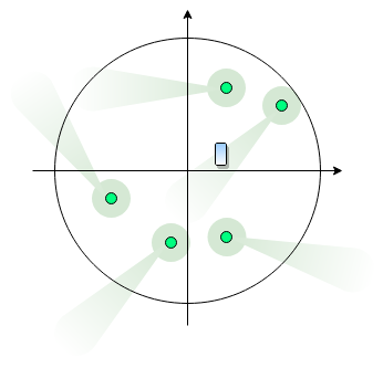
Figure 5: Snapshot of the indoor mmWave hotspot layout with five transmitters. The reference receiver location is marked with a rectangle and the transmitter locations are the small circles. The direction of transmissions for all the transmitters is illustrated as rotation of the 2D- projection of the cone bulb antenna gain model in (4).

In the following we will first look at the network design implications coming from our model and consider the impact that the number of transmitters and their antenna directionality have on the system performance. We perform our numerical analysis for an idealistic case, assuming that our serving transmitter is at a horizontal distance of 1 m away from the reference receiver (which, as we will show later, allows us to meet ATC and EDR targets for most of the analysed scenarios), with its main beam being fully aligned with the receiver beam, and an LOS channel between the two. Subsequently, we will re-visit these assumptions and consider how network performance changes with increased distance to the serving transmitter and when the reference link is in NLOS state.

III-D2 Network performance

First let us consider how the results we obtained compare to the performance requirements imposed on the 3GPP Indoor Hotspot scenario. Following the chairman of the 3GPP system architecture group [53], these include 1 Gbit/s of EDR, and 15 $\text{Tbps/km}^{2}$ of ATC, both in the downlink direction. As we can see from Fig. 6, whether or not we meet the performance targets is highly dependent on the usage scenario. Broadly speaking, scenarios where the user device is held further away from the user body achieve the ATC target with 4 transmitters in a given area and maintain values higher than target EDR for all of the considered network densities. The reason for this is low path attenuation at the reference distance. For that same reason Hallway pocket scenario meets target requirements. The other scenarios require double the number of transmitters to achieve the same performance, but, critically, do not offer target EDR.

Looking at Fig. 6(a) we see that the increasing number of transmitters leads to linear increase in ATC, which, given the expression in (9), comes from the linear increases in the number of available infrastructure per unit area. Due to relatively narrow beams that we use, $\omega_{\mathrm{TX}}=30\degree$, this densification does not lead to increase in interference, which can be confirmed by observing almost flat EDR curves in Fig. 6(b) (which illustrates the performance of users that would suffer the most if any increase in interference occurred). The coverage plots in Fig. 6(c) show the exact same story providing us with almost flat lines for each of the considered scenarios. In conclusion, we see that for the selected network setup our network operates in the noise-limited regime for all of the usage scenarios with the exception of the Hallway app that is characterized by low reference distance path attenuation.

Another way to bring the data rates up would require that we increase the antenna gains by using narrower beams, either on the transmitter (as shown in Fig. 7), or the receiver side. Beamwidth has a much more critical impact on both the ATC and EDR. In Fig. 7(b), we can see that for some of the scenarios the EDR drops to values below what, for example, an average LTE (LTE) user would experience. In order to ensure that users under all usage scenarios enjoy target EDR would require that we use transmitter beamwidths far below our default configuration of 30 $\degree$. Wider beams produce significant interference which greatly reduces the performance of the worst-off users for the three scenarios with high reference distance path attenuation. However, in the other three scenarios while the performance reduces it does so only to a lesser degree and ATC stays above the target performance for all beamwidths considered.

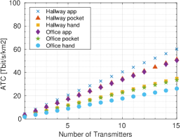
(a) ATC

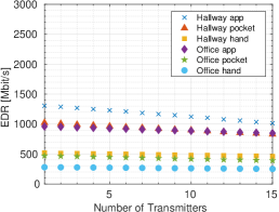
(b) EDR

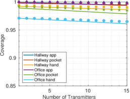
(c) Coverage

Figure 6: Impact of the number of transmitters $n_{\mathrm{TX}}$. Where $n_{\mathrm{TX}}=1$ represents the scenario with a single serving transmitter and no other transmitters within a given area. Other network settings are: $\omega_{\mathrm{TX}}=\text{30\,$\degree$}$, $r_{0}=\text{1\,m}$, and $p_{\mathrm{LOS}}=0.5$.

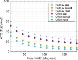
(a) ATC

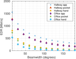
(b) EDR

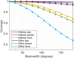
(c) Coverage

Figure 7: Impact of the transmitter antenna main-lobe width $\omega_{\mathrm{TX}}$. The antenna gain scales with $\omega_{\mathrm{TX}}$ according to (4). Other network settings $n_{\mathrm{TX}}=12$, $r_{0}=\text{1\,m}$, and $p_{\mathrm{LOS}}=0.5$.

When it comes to coverage (see Fig. 6(c) and Fig. 7(c)) we should remark that—as one would expect—increasing the number of transmitters deteriorates coverage. In Fig. 6(c), coverage degrades linearly with the number of transmitters, albeit at a negligibly small rate. This is good news as it means that the resulting interference may be low enough to not warrant the need for interference coordination, at least as long as directionalities of transmissions are independent across space, an observation also made for large-scale, outdoor mmWave networks [54]. The choice of the beamwidth has a more critical impact on the coverage performance, in Fig. 7(c). If the coverage is to be kept at (or above) 90% mark for all of the scenarios, it is necessary that the transmitter beamwidth stays at (or below) roughly 60 $\degree$, as wider beams may produce unmitigated interference. Interestingly, when beams of 50 $\degree$ or more are used, we start seeing differences in coverage between the scenarios. Similarly to changes in ATC and EDR performance this can be explained by high discrepancy in the path attenuation at the reference distance between the usage scenarios.

III-D3 Network performance under design imperfections

In Fig. 8 we consider the horizontal distance to the serving transmitter. In practical cases a particular cell will serve a particular user. This means the serving distance may not depend on the density of transmitters or receivers. In Fig. 8 we see that all our performance characteristics degrade with the serving distance. The serving distance is especially critical for the coverage, as in four of our usage cases the coverage goes below the 90% mark at roughly 5 m horizontal distance already. Interestingly this does not affect the ATC performance which stays at relatively high values even at longer serving distances. Yet, the performance of worst-off users becomes highly volatile to change in their distance to the serving transmitter, and all of our scenarios fall below the 1 Gbit/s target beyond the horizontal distance of 2 m.

We are also interested in testing how the performance changes when the reference link is in blockage state caused by the user body. In Fig. 9 we see – following intuition – that LOS blockage leads to performance degradation. While the coverage is affected only in a minor way, for each of the scenarios network performance, interpreted as ATC, drops below the performance targets, in the cases where body blockage is high (Hallway app, Hallway pocket, and Office app) dropping by as much as 70%. But more critically, the 5^th percentile user throughput becomes only a small fraction of the LOS case. This is an important observation that motivates work into blockage mitigation strategies: [55, 56, 57]. In our studies we also considered the impact of blockage probability. However, for the setup we used to evaluate our system, the disparity between LOS and NLOS channels on the interfering links was not strong enough to yield any significant differences in performance. We can conclude that while body blockage does indeed introduce significant attenuation to interfering links (see body blockage values in Table I), in a well-designed network with the carefully chosen beamwidths and a reasonable number of transmitters it should not affect network performance.

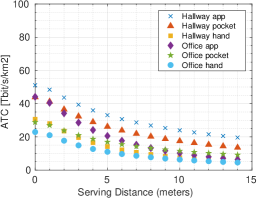
(a) ATC

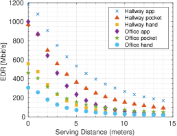
(b) EDR

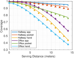
(c) Coverage

Figure 8: Impact of the serving distance. Other network settings $n_{\mathrm{TX}}=11$, $\omega_{\mathrm{TX}}=\text{30\,$\degree$}$, and $p_{\mathrm{LOS}}=.5$.

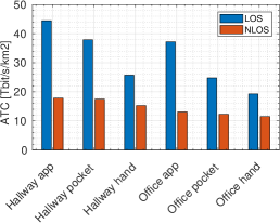
(a) ATC

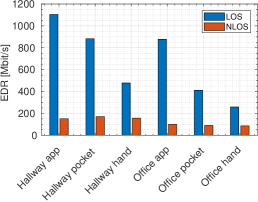
(b) EDR

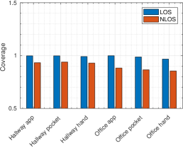
(c) Coverage

Figure 9: Impact of the reference link blockage. Other network settings $n_{\mathrm{TX}}=11$, $\omega_{\mathrm{TX}}=\text{30\,$\degree$}$, $r_{0}=\text{1\,m}$, and $p_{\mathrm{LOS}}=.5$.

Since beam management is also a fundamental aspect to consider in mmWave systems [58], in our numerical evaluations we also considered the impact of beam misalignments. Given our system setup, we have observed that any misalignment between transmitter and receiver beams substantially throttles any communication links between the two, reducing coverage to almost zero. While this result motivates strong need for accurate beam alignment procedures, such as [59], it is also based on a pessimistic antenna pattern model that incorporates sharp degradation in performance in case of any misalignments. With realistic antenna patterns, misalignments should lead to a more gradual performance degradation [60], impact of which would require further studies.

IV Deployment Analysis

Section III has addressed system-level modeling and performance evaluation. These tasks are critical to understanding the basic factors that will impact the performance of mmWave deployments across a variety of scenarios. They help us to answer questions about the impact of factors such as base station density, antenna beamwidth, and serving distance on various measures of performance. Nevertheless, after examining these results, actual deployment planning for specific environments remains a challenge in mmWave systems.

In a particular environment, deployment is constrained first by the set of possible AP locations. Then, it is necessary for deployment to consider many of the same factors considered in the analysis in Section III. Namely, issues such as beamwidth and planned serving distance must be considered. In addition, we saw in the last section that whether a link is LOS or NLOS has a significant impact on system performance. For a particular deployment, the issue of LOS vs. NLOS will depend on the location of the AP, user device orientation, as well as orientations of all human bodies in the considered space, including that of the device user.

In this section, we discuss efficient schemes for AP deployment and beam steering in mmWave networks. In particular, given a set of possible AP locations, we setup a stochastic optimization problem to determine the best set of AP locations, as well as the best directions to aim the AP’ beams in order to meet coverage requirements while minimizing the deployment cost. We use a stochastic optimization problem to model the fact that the set of user locations at any given time is uncertain, but can be modeled as the realization of a point process. For the purposes of this paper, we step beyond the recent work on mmWave AP deployment by assuming that each AP generates multiple, fixed beams; dynamic beam management is left for future work.

There have been some recent works on AP deployment in mmWave networks, such as [61, 62, 63, 64]. However, these works neither consider the beam steering problem nor account for the uncertainty in user locations. In [61], the authors proposed an automated scheme for placing mmWave AP and gathering their line-of-sight coverage statistics, to help model small-cell mmWave access networks. Considering the deafness and blockage problems in mmWave networks, in [62, 63] the authors proposed distributed schemes for association and relaying that improve network throughput. In another AP deployment scheme, [64], the authors assumed that APs always direct their beams in one fixed direction and considered a fixed set of UE with static locations. In contrast, we assume fixed beam directions, but we assume that each AP can generate multiple beams.

Considering uncertainty in the availability of mmWave links between AP and UE, combined with user location uncertainty, in this section we describe a CCSP (CCSP) [65] framework for joint AP deployment and beam steering in mmWave networks, called DBmWave. CCSP has been recently used to model several resource allocation problems in uncertain networks [66, 67, 68]. DBmWave aims at minimizing the required number of mmWave AP to achieve a minimum network-wide coverage probability of $\beta$, which represents the requested QoS (QoS) level. The network-wide coverage probability constraint formulated in this paper is in contrast to the per-user coverage probability constraint formulated in [64]. Instead of formulating a constraint for each user to ensure that individual users are covered with a minimum probability $\beta$, we formulate a single constraint for the entire mmWave network that ensures that any arbitrarily selected user will be covered with this minimum probability $\beta$. Using various reformulation techniques, we equivalently reformulate our stochastic program as a BLP (BLP). Finally, we numerically analyze the performance of DBmWave under various system settings.

Note that in addition to user location, because of significant human body shadowing in mmWave networks, user orientation is also a significant source of uncertainty. We have addressed this in some past work [64] and may integrate such considerations into this work in the future.

IV-A System Model

We consider a three-dimensional geographical area with a set $\mathcal{N}=\{1,2,\ldots,N\}$ of candidate locations for deploying mmWave AP on the ceiling to cover the floor, as depicted in Fig. 10. The floor is divided into $K=\frac{r_{d}}{2\;r_{b}}+\frac{1}{2}$ annuli, the $i$th annulus consists of $M_{i}$ circles, where $M_{i}$ is given by:

$$M_{i}=\Bigg{\lfloor}\frac{2\pi}{2\sin^{-1}\left(\frac{r_{b}}{r_{d}-2\;r_{b}(K-i)-r_{b}}\right)}\Bigg{\rfloor}=\Bigg{\lfloor}\frac{\pi}{\sin^{-1}\left(\frac{1}{2(i-1)}\right)}\Bigg{\rfloor}.$$ (16)

$r_{d}$ represents the radius of the geographical area and $r_{b}$ is the radius of each circular area, as depicted in Fig. 10. We denote the set of circular areas by $\mathcal{K}$, where $|\mathcal{K}|=1+\sum_{i=2}^{\frac{r_{d}}{2\;r_{b}}+\frac{1}{2}}M_{i}$. The $k$th circular area in $\mathcal{K}$, denoted by $A_{k}$, is represented by a pair $(i_{k},j_{k})$, as illustrated in Fig. 10.

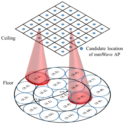
Figure 10: Illustration of the system model considered in DBmWave.

UE are distributed in the geographical area according to the distribution $f_{Z}(z)$. The link between a mmWave AP placed at location $n\in\mathcal{N}$ and the $k$th circular area, $k\in\mathcal{K}$, if one of the AP beams is steered to cover $A_{k}$, is only available with probability $p_{nk}$. The maximum number of beams that a mmWave AP can have is denoted by $B$.

IV-B Problem Statement

Given $\mathcal{N}$, $\mathcal{K}$, $B$, $\beta$, $f_{Z}(z)$, and $p_{nk},n\in\mathcal{N},k\in\mathcal{K}$, we answer the following questions jointly while ensuring that an arbitrarily chosen user within the geographical area of interest will be covered with a probability $\geq\beta\in(0,1)$.

1. What is the minimum number of required mmWave AP?

2. How can they be deployed optimally?

3. How can their beams be steered optimally?

IV-C Problem Formulation

Let $y_{nk},n\in\mathcal{N},k\in\mathcal{K}$, be binary decision variables; $y_{nk}$ equals one if a mmWave AP is placed at location $n$ and one of its beams is steered to cover region $k$, and it equals zero otherwise. Let $\mathbb{P}_{\text{cov}}$ be the network-wide coverage probability, i.e., the probability that an arbitrarily selected user in the network will be covered. Then, the joint AP deployment and beam steering problem can be formulated as:

where $\mathds{1}_{\{\cdot\}}$ is an indicator function; $\mathds{1}_{\{\cdot\}}$ equals one if $\{\cdot\}$ is satisfied and zero otherwise, and $\beta\in(0,1)$.

IV-C1 Coverage Probability Constraint

As stated earlier, the coverage probability is defined as the probability that an arbitrarily selected user lies in a circular area that is covered by at least one active beam. Hence, the coverage probability when the arbitrarily selected user is located at $z$ can be defined as:

$$\mathbb{P}_{\text{cov}}^{(z)}=\mathbb{E}\left[1-\prod_{n\in\mathcal{N}}\left(1-\delta_{nk^{(z)}}y_{nk}\right)\right],$$ (21)

where $k^{(z)}$ is the index of the circular area that contains location $z$. $\delta_{nk^{(z)}}$ equals one if there is no blockage between the AP candidate location $n$ and the circular area $A_{k^{(z)}}$, and it equals zero otherwise. The expectation in (21) is over blockages, which—similarly to Section III— are assumed to be independent across links. Therefore,

$$\mathbb{P}_{\text{cov}}^{(z)}=1-\prod_{n\in\mathcal{N}}\left(1-p_{nk^{(z)}}y_{nk}\right).$$ (22)

To compute the unconditioned coverage probability, we take the user distribution $f_{Z}(z)$ into consideration as follows:

$$\mathbb{P}_{\text{cov}} =1-\sum_{k\in\mathcal{K}}\left(\int_{A_{k}}f_{Z}(z)\;{\rm d}z\prod_{n\in\mathcal{N}}\left(1-p_{nk}\;y_{nk}\right)\right).$$ (23)

The integration $\int_{A_{k}}f_{Z}(z)\;{\rm d}z$ over each circular area is upper-bounded by the integration over the sector enclosed in the $i_{k}$-th annulus between the two tangents of $A_{k}$, see (IV-C1). This upper bound is used in our analysis to enhance tractability. This enables us to use the probability distribution $f_{R_{z}}(r_{z})$, where $R_{z}=\|z\|$. The term $\left(2\sin^{-1}\left(\frac{1}{2(i_{k}-1)}\right)\right)$ in (IV-C1) represents the angle of the sector enclosed in the $i_{k}$-th annulus between the two tangents of $A_{k}$. The term $a_{i_{k}}$ is added to ensure that $\sum_{k\in\mathcal{K}}\int_{A_{k}}f_{Z}(z)=1$. In Section IV-D, the following two user distributions are investigated:

• Truncated Gaussian distribution, where $f_{R_{z}}^{\rm gaus}(r_{z})=\frac{r_{z}\exp\left(-\frac{r_{z}^{2}}{2\sigma^{2}}\right)}{\sigma^{2}\left(1-\exp\left(-\frac{r_{d}^{2}}{2\sigma^{2}}\right)\right)}$ and $\sigma^{2}$ represents the variance of the user distribution.

• Uniform distribution, where $f_{R_{z}}^{\rm unif}(r_{z})=\frac{2r_{z}}{r_{d}^{2}}$.

$$\int_{A_{k}}f_{Z}(z)\;{\rm d}z \leq\left(a_{i_{k}}+2\sin^{-1}\left(\frac{1}{2(i_{k}-1)}\right)\right)\int_{r_{d}-2r_{b}(K-i_{k}+1)}^{r_{d}-2r_{b}(K-i_{k})}\frac{f_{R_{z}}(r_{z})}{2\pi}\;{\rm d}r_{z}$$

$$=\left(a_{i_{k}}+2\sin^{-1}\left(\frac{1}{2(i_{k}-1)}\right)\right)\int_{2r_{b}(i_{k}-1.5)}^{2r_{b}(i_{k}-0.5)}\frac{f_{R_{z}}(r_{z})}{2\pi}\;{\rm d}r_{z},$$

$$\hskip 216.81pt\forall 2\leq i_{k}\leq K.$$ (24)

 

IV-C2 Equivalent BLP

First, note that the objective function of Problem 1 is non-linear. It can be represented in a linear form by introducing new binary decision variables, $x_{n}\triangleq\mathds{1}_{\left\{\sum_{k\in\mathcal{K}}y_{nk}\geq 1\right\}},\forall n\in\mathcal{N}$, and reformulating the indicator function as follows [69]:

• If $\sum_{k\in\mathcal{K}}y_{nk}\geq 1$ then $x_{n}=1$ can be reformulated as:

  $$\sum_{k\in\mathcal{K}}y_{nk}-\left(M+\epsilon\right)x_{n}\leq 1-\epsilon,$$ (25)

  where $M$ is an upper bound of $\sum_{k\in\mathcal{K}}y_{nk}-1$ and $\epsilon>0$ is a small tolerance beyond which we regard the constraint as having been broken. Selecting $M$ and $\epsilon$ to be $B-1$ and $1$, respectively, (25) reduces to $\sum_{k\in\mathcal{K}}y_{nk}\leq B\;x_{n}$.

• If $x_{n}=1$ then $\sum_{k\in\mathcal{K}}y_{nk}\geq 1$ can be reformulated as:

  $$\sum_{k\in\mathcal{K}}y_{nk}+m\;x_{n}\geq m+1,$$ (26)

  where $m$ is a lower bound of $\sum_{k\in\mathcal{K}}y_{nk}-1$. Selecting $m$ to be $-1$, (26) reduces to $\sum_{k\in\mathcal{K}}y_{nk}\geq x_{n}$.

Therefore,

$$x_{n}=\mathds{1}_{\left\{\sum_{k\in\mathcal{K}}y_{nk}\geq 1\right\}}\;\Longleftrightarrow\;x_{n}\leq\sum_{k\in\mathcal{K}}y_{nk}\leq B\;x_{n},\forall n\in\mathcal{N}.$$

Second, the coverage probability expression, $\mathbb{P}_{\text{cov}}$, has the term $\mathbb{P}\triangleq\prod_{n\in\mathcal{N}}\left(1-p_{nk}\;y_{nk}\right)$, which is nonlinear in the decision variables $y_{nk},n\in\mathcal{N},k\in\mathcal{K}$. Expanding $\mathbb{P}$, we can see that the nonlinear terms in $\mathbb{P}$ are in the form of products of binary decision variables. For example, if $N=3$, $\mathbb{P}$ can be expressed as:

$$\mathbb{P}=1-\sum_{i=1}^{3}p_{ik}\;y_{ik}+p_{1k}\;p_{2k}\;y_{1k}\;y_{2k}+p_{1k}\;p_{3k}\;y_{1k}\;y_{3k}+p_{2k}\;p_{3k}\;y_{2k}\;y_{3k}-\prod_{i=1}^{3}p_{ik}\;y_{ik}.$$ (27)

To linearize a product of binary decision variables, say $\prod_{i=1}^{N}y_{ik}$, we introduce a new auxiliary non-negative decision variable, say $y_{k}$, replace $\prod_{i=1}^{N}y_{ik}$ by $y_{k}$, and add the following constraints:

$$y_{k}\leq y_{ik},\forall i\in\{1,2,\ldots,N\}$$

$$y_{k}\geq\sum_{i=1}^{N}y_{ik}-\left(N-1\right)$$

$$y_{k}\geq 0.$$ (28)

After reformulating the indicator function and $\mathbb{P}$, as explained above, Problem 1 becomes a BLP.

IV-D Numerical Analysis

IV-D1 Setup

Assuming an open indoor environment, $r_{d}$ and $r_{b}$ were selected to be 5.5 and 0.5 meters, respectively. Based on these values, we calculated the number of circular areas, as explained in subsection IV-A, and found that $K=92$. The maximum number of beams that a mmWave AP can have, $B$, is varied between $1$ and $4$. The AP are assumed to be mounted on the ceiling, which is $10\times 10$ m². The height of the ceiling is assumed to be 3 m, similarly to our measurement setup in Sections II and III. The AP are deployed in a grid-based manner, similarly to the indoor hotspot scenario presented in [17], that is, each candidate location is with equal distance to each other, as shown in Fig. 10. Two different user distributions were considered: (i) Gaussian distribution with mean $u=0$ and variance $\sigma=10$ and (ii) uniform distribution. The probabilities of link availability were calculated assuming three channel effects: path loss, small-scale fading, and blockage (the event of a user having no LOS with a certain AP). We adopt the power-law path loss model, as presented in (1). For LOS case, we set $P_{0}$ to $78.31$ dB and $n$ to $2.1$. For NLOS case, we set $P_{0}$ to $95.39$ dB and $n$ to $3.5$. We set $d_{0}$ to $1$ m.

The small-scale fading is assumed to follow the $\kappa-\mu$ distribution given by (2). For LOS case, we set $\kappa$ to $2.80$, $\mu$ to $0.77$, and $\Omega$ to $1.16$. For NLOS case, we set $\kappa$ to $0.92$, $\mu$ to $0.96$, and $\Omega$ to $1.23$.

Similarly to Section III, blockages across the links between the mmWave AP and the coverage areas are modelled as independent and identically distributed (i.i.d.) Bernoulli random variables. $p_{LOS}$ denotes the probability that there is no blockage on a certain link between an AP and a coverage area and $p_{NLOS}=1-p_{LOS}$ denotes the probability that there is a blockage on the link. In general, $p_{LOS}$ varies from one link to another; for our numerical results, $p_{LOS}$ is set to $0.5$ for all the links. Moreover, given the results in Fig. 6 which showed negligibly small degradation of coverage in response to the increasing number of transmitters and similarity in system parameters, we can assume that frequency reuse factor is $\ll 1$, i.e., interference is negligible. The Gaussian noise spectral density is set to -174 dBm/Hz.

While linearizing Problem 1 above, we assumed that, for each user, there are only three AP candidate locations that can cover it. These three AP locations form the best (most available) AP-user links (i.e., links with the highest $p_{n,k}$ values for a given $k$). We selected different values of $N$, the number of AP candidate locations, to better characterize the behavior of the system. We evaluated our stochastic optimization framework in terms of the required number of AP for different coverage probabilities $\beta$. The optimization problem was solved using CPLEX.

IV-D2 Results

Fig. 11(a) shows the number of required APs as a function of the minimum required coverage probability ($\beta$). In this figure, the number of AP candidate locations was chosen to be $N=100$, the users were assumed to be distributed according to a Gaussian distribution. It can be seen that as $\beta$ increases, more AP are needed to satisfy the coverage demand. Furthermore, increasing the number of beams at each AP reduces the required number of AP. This is expected, as having more beams at an AP allows it to cover more users.

Fig. 11(b) is similar to Fig. 11(a), but assuming the users to be uniformly distributed. Both figures show similar trends. However, the number of AP required to satisfy a certain coverage probability is higher when the users are uniformly distributed. In the case of Gaussian distribution, users are clustered in the geographical area (in contrast to the case of uniform distribution). This clustering results in reducing the number of required AP.

Finally, Fig. 11(c) illustrates the effect of the number of AP candidate locations on the number of required AP to meet a certain coverage probability. It can be seen that as $N$ increases the number of required AP decreases. This is due to the fact that increasing $N$ expands the feasibility region of the allocation problem, opening the room for better solutions (i.e., with lower objective function value).

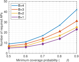
(a)

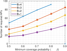
(b)

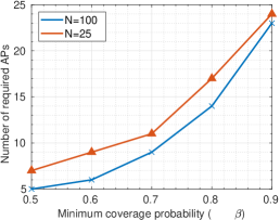
(c)

Figure 11: Number of required AP vs. minimum coverage probability for: a) Gaussian distributed users, with $N=100$ beams, b) uniformly distributed users, with $N=100$ beams, and c) Gaussian distributed users and different values of $N$, with $B=4$.

V Discussion and Concluding Remarks

In the preceding sections we described findings that pertain to various aspects of indoor mmWave network design. Crucially, we showed that indoor mmWave deployments may achieve (or come close to achieving) performance targets of 1 Gbit/s EDR, and 15 $\text{Tbps/km}^{2}$ ATC [53]. Yet, this performance can be volatile to device usage scenarios. In this section, we bring together the results to discuss these trade-offs, and look more closely at any outstanding challenges.

V-A Take Away Lessons

In the system-level analysis, we saw that our reference user achieved almost 100% coverage, even under the presence of body blockages, in Fig. 9(c). From the deployment analysis in Fig. 11(a) and Fig. 11(b), we saw that this does not need to be the case if multiple users are considered. Covering each and every user above a certain reliability threshold may require deploying an excessively large number of access points, especially if we expect high reliability. These additional transmitters will increase the network capacity, see Fig. 6(a), without deteriorating the rate for 5^th percentile users, see Fig. 6(b). However, depending on the usage scenario these 5^th percentile users may operate substantially below the required performance. In Section IV, we showed that this can be avoided by coordinating deployment locations and beam steering according to the patterns of user locations (users that cluster in space) and user orientations (users that face single direction). This can be observed by comparing results in Fig. 11(a) and Fig. 11(b).

Another way to bring up the 5^th percentile user performance is to increase the antenna gain by narrowing the transmission beamwidth, as we showed in Fig. 7(b). This will come at a cost of using more directional antennas or antenna arrays with larger number of components, and a potential reduction in the performance of beam tracking and alignment mechanisms, which require wider beams to operate (as reported in, e.g., [59]). This trade-off in beamwidth design can be avoided by planning for a deployment with less stringent coverage reliability requirements, which, as we could observe in Fig. 11(a), greatly reduces the number of necessary transmitters, leading to reduced interference and enabling us the usage of wider beams.

V-B Future Challenges

V-B1 Exploiting Differences in Channel Characteristics Across Multiple Frequency Bands

One way to improve link availability in mmWave networks is to make use of dual connectivity at microwave and mmWave operating frequencies [70]. To fully exploit the extra degree of freedom offered through dual-band operation, channel characteristics of both connections should be adequately de-correlated (i.e., if the mmWave link goes into outage due to shadowing or a deep fade, then it would be anticipated, that under normal circumstances, the microwave link should act to provide a more reliable fall-back service). At present, we have a fairly good overall understanding of the quantitative differences in propagation within the microwave and mmWave regions of the radio spectrum [71]. Nonetheless, important channel metrics such as the correlation in shadowing and multipath fading across frequency bands (introduced by human body blockages) is still largely uncharted territory, e.g., [20]. To ensure that the instantaneous channel characteristics are suitably disparate for the envisaged multi-band operation, extensive channel measurement campaigns, as well as follow-up system-level analyses will be necessary.

V-B2 Coexistence between 5G-NR and WiFi

One of the key issues to address when operating in mmWave unlicensed bands is coexistence with other wireless systems. For example, in the 60 GHz band where the 3GPP is planning to deploy NR-U, mechanisms will have to be developed to enable coexistence with wireless local area networks like the IEEE Wireless Gigabit 802.11ad/ay [5, 6]. As a matter of fact, the ETSI (ETSI) has already published a list of conformance requirements, which include limits on the maximum emitted power or channel sensing mechanisms, necessary to ensure fair coexistence between the systems operating in unlicensed mmWave bands [72]. Yet, more work is needed to understand the impact of these coexistence rules on the network performance and, ultimately, network design.

V-B3 Network Densification Limits

Finally, in Fig. 6(a), we could see that the network capacity of our system increases with the number of transmitters. An interesting question is to ask about the asymptotic case, and the limits of network densification. In [73], it was observed that network densification is limited by the channel characteristics, and antenna heights. However, this result applies to networks operating over large areas and network settings that correspond to outdoor deployments, e.g., variable deployment heights of tens of meters above ground level. One would expect that for ceiling-mounted mmWave networks, with highly directional beams, we can reach high deployment densities, without making the system interference-limited, and thus achieve high network capacities. Yet, this would make beam alignment and tracking more challenging, thus potentially limiting the achievable network capacity. Analysis of this network density asymptotic regime would likely require a new modelling framework.

Appendix A Proof of Lemma 1

The power received at the reference user (as provided in (6)), conditioned on the blockage state $t$ and antenna gain $g_{i}$, is a product of the fading random variable and a constant. This allows us to express the PDF of $S_{i,t}$ using (5)

$$f_{S_{i,t}}(s)=\frac{\theta_{1}^{(\mu+1)/2}}{\vartheta_{i,t}^{(\mu+1)/2}\theta_{2}^{(\mu-1)/2}}s^{(\mu-1)/2}\exp\left(-\frac{\theta_{1}}{\vartheta_{i,t}}s-\theta_{2,t}\right)I_{\mu_{t}-1}\left(2\sqrt{\frac{\theta_{1,t}\theta_{2,t}s}{\vartheta_{i,t}}}\right),$$ (29)

where $\vartheta_{i,t}=g_{i}l_{t}\left(r_{i}\right)$, and $I_{\mu_{t}-1}$ is the modified Bessel function of the first kind and order $\mu_{t}-1$. Now, using the series representation of the modified Bessel function we get that

$$f_{S_{i,t}}(s)=\frac{\theta_{1,t}^{\mu_{t}}\exp(-\theta_{2,t})}{\vartheta_{i,t}^{\mu_{t}}}\sum_{l=0}^{\infty}\frac{\theta_{1,t}^{l}\theta_{2,t}^{l}}{\vartheta_{i,t}^{l}\Gamma(\mu_{t}+l)l!}s^{\mu_{t}-1+l}\exp\left(-\frac{\theta_{1,t}}{\vartheta_{i,t}}s\right).$$ (30)

Then the CDF of $S_{i,t}$ can be expressed as

$$\begin{split}\mathbb{P}\left(S_{i,t}>x\right)&=\int_{x}^{\infty}f_{S_{i,t}}(s)\differential{s}\\ &\overset{(a)}{=}\frac{\theta_{1,t}^{\mu_{t}}\exp(-\theta_{2,t})}{\vartheta_{i,t}^{\mu_{t}}}\sum_{l=0}^{\infty}\frac{\theta_{1,t}^{l}\theta_{2,t}^{l}}{\vartheta_{i,t}^{l}\Gamma(\mu_{t}+l)l!}\int_{x}^{\infty}s^{\mu_{t}-1+l}\exp\left(-\frac{\theta_{1,t}}{\vartheta_{i,t}}s\right)\differential{s}\\ &=\exp(-\theta_{2,t})\sum_{l=0}^{\infty}\frac{\theta_{2,t}^{l}}{l!}\frac{\Gamma(l+\mu_{t},\frac{\theta_{1,t}}{\vartheta_{i,t}}x)}{\Gamma(l+\mu_{t})}\\ &\overset{(b)}{=}\exp(-\theta_{2,t})\sum_{l=0}^{\infty}\frac{\theta_{2,t}^{l}}{l!}\sum_{n=0}^{l+\mu_{t}-1}\frac{1}{n!}\left(\frac{\theta_{1,t}x}{\vartheta_{i,t}}\right)^{n}\exp\left(-\frac{\theta_{1,t}}{\vartheta_{i,t}}x\right),\end{split}$$ (31)

where for (a) we use the expression in (30), and (b) holds only for the special case of $\mu_{t}$ being a positive integer.

Appendix B Proof of Lemma 2

In the following, given the distance to the serving transmitter $r_{0}$, serving link gain $g_{0}$, and the serving channel being in state $t$, and denoting the longer-term average power received from the serving transmitter as $\vartheta_{0,t}=g_{0}l_{t}\left(r_{0}\right)$, we derive the conditional CCDF of the SINR as experienced by the reference user, i.e., $\mathbb{P}_{\text{cov}}=F^{c}_{\mathrm{SINR}|R_{0},G_{0},T}\left(\zeta|r_{0},g_{0},t\right)$. For a given threshold $\zeta$, this conditional CCDF can be defined as

$$\begin{split}\mathbb{P}_{\text{cov}}&=\mathbb{P}\left(S>\zeta\cdot\left(I+\tau^{-1}\right)\right)\\ &=\exp(-\theta_{2,t})\sum_{l=0}^{\infty}\frac{\theta_{2,t}^{l}}{l!}\sum_{n=0}^{l+\mu_{t}-1}\frac{\mathbb{E}[(\frac{\zeta\theta_{1,t}}{\vartheta_{0,t}}\left(I+\tau^{-1}\right))^{n}\exp\left(-\frac{\zeta\theta_{1,t}}{\vartheta_{0,t}}\left(I+\tau^{-1}\right)\right)]}{n!}\\ &\overset{(a)}{=}\exp\left(-\theta_{2,t}-\frac{\zeta\theta_{1,t}}{\vartheta_{0,t}\tau}\right)\sum_{l=0}^{\infty}\frac{\theta_{2,t}^{l}}{l!}\sum_{n=0}^{l+\mu_{t}-1}\frac{1}{n!}\left(\frac{\zeta\theta_{1,t}}{\vartheta_{0,t}}\right)^{n}\sum_{k=0}^{n}{n\choose k}\tau^{-n+k}\mathbb{E}[I^{k}\exp\left(-\frac{\zeta\theta_{1,t}}{\vartheta_{0,t}}I\right)]\\ &=\exp\left(-\theta_{2,t}-\frac{\zeta\theta_{1,t}}{\vartheta_{0,t}\tau}\right)\sum_{l=0}^{\infty}\frac{\theta_{2,t}^{l}}{l!}\sum_{n=0}^{l+\mu_{t}-1}\frac{1}{n!}\left(\frac{\zeta\theta_{1,t}}{\vartheta_{0,t}\tau}\right)^{n}\sum_{k=0}^{n}{n\choose k}\tau^{k}\\ &\mathbb{E}\left[\left(\sum^{n_{\mathrm{TX}}}_{i=1}G_{i}H_{i,V}l_{V}(R_{i})\right)^{k}\exp\left(-\frac{\zeta\theta_{1,t}}{\vartheta_{0,t}}\left(\sum^{n_{\mathrm{TX}}}_{i=1}G_{i}H_{i,V}l_{V}(R_{i})\right)\right)\right]\\ &\overset{(b)}{=}\exp\left(-\theta_{2,t}-\frac{\zeta\theta_{1,t}}{\vartheta_{0,t}\tau}\right)\sum_{l=0}^{\infty}\frac{\theta_{2,t}^{l}}{l!}\sum_{n=0}^{l+\mu_{t}-1}\frac{1}{n!}\left(\frac{\zeta\theta_{1,t}}{\vartheta_{0,t}\tau}\right)^{n}\sum_{k=0}^{n}{n\choose k}\tau^{k}\\ &\sum_{k_{1}+k_{2}+\ldots+k_{n_{\mathrm{TX}}}=k}{k\choose k_{1},k_{2},\ldots,k_{n_{\mathrm{TX}}}}\prod_{1\leq i\leq n_{\mathrm{TX}}}\mathbb{E}\left[\left(G_{i}H_{i,V}l_{V}(R_{i})\right)^{k_{i}}\exp\left(-\frac{\zeta\theta_{1,t}}{\vartheta_{0,t}}G_{i}H_{i,V}l_{V}(R_{i})\right)\right]\\ &\overset{(c)}{=}\exp\left(-\theta_{2,t}-\frac{\zeta\theta_{1,t}}{\vartheta_{0,t}\tau}\right)\sum_{l=0}^{\infty}\frac{\theta_{2,t}^{l}}{l!}\sum_{n=0}^{l+\mu_{t}-1}\frac{1}{n!}\left(\frac{\zeta\theta_{1,t}}{\vartheta_{0,t}\tau}\right)^{n}\sum_{k=0}^{n}{n\choose k}\tau^{k}\sum_{k_{1}+k_{2}+\ldots+k_{n_{\mathrm{TX}}}=k}{k\choose k_{1},k_{2},\ldots,k_{n_{\mathrm{TX}}}}\\ &\prod_{1\leq i\leq n_{\mathrm{TX}}}\underbrace{\mathbb{E}_{V,G_{i},R_{i}}\left[\frac{(\mu_{V})_{k_{i}}\theta_{1,V}^{\mu_{V}}\exp(-\theta_{2,V})\left(G_{i}l_{V}(R_{i})\right)^{k_{i}}}{\left(\frac{\zeta\theta_{1,t}}{\vartheta_{0,t}}G_{i}l_{V}(R_{i})+\theta_{1,V}\right)^{k_{i}+\mu_{V}}}\mbox{${}_{1}$F${}_{1}$}\left(k_{i}+\mu_{V};\mu_{V};\frac{\theta_{1,V}\theta_{2,V}}{\frac{\zeta\theta_{1,t}}{\vartheta_{0,t}}G_{i}l_{V}(R_{i})+\theta_{1,V}}\right)\right]}_{\mathbb{I}_{1}},\end{split}$$ (32)

where (a) comes from the binomial expansion, in (b) we apply the multinomial expansion and use the fact that antenna gains, channel fading, and distances are independent across all the interferers, (c) comes from taking the expectation with respect to the fading random variable (one can find it by either considering series representation of the PDF of fading or considering the integral in [74][Eq. 6.643.2]).

Now, the expectation in the expression above captures three (at least potentially) random parameters of any interfering transmitter, which are the blockage state, directionality and distance, and can be repesented as:

$$\begin{split}\mathbb{I}_{1}&=\sum_{v\in\{\mathrm{LOS},\mathrm{NLOS}\}}p_{v}\sum_{g\in\mathcal{G}}p_{g}(\mu_{v})_{k_{i}}\theta_{1,v}^{\mu_{v}}g^{k_{i}}\exp(-\theta_{2,v})\times\\ &\mathbb{E}_{R}\Big{[}\frac{l_{v}^{k_{i}}(R)}{\left(\frac{\zeta\theta_{1,t}}{\vartheta_{0,t}}gl_{v}(R)+\theta_{1,v}\right)^{k_{i}+\mu_{v}}}\mbox{${}_{1}$F${}_{1}$}\left(k_{i}+\mu_{v};\mu_{v};\frac{\theta_{1,v}\theta_{2,v}}{\frac{\zeta\theta_{1,t}}{\vartheta_{0,t}}gl_{v}(R)+\theta_{1,v}}\right)\Big{]},\end{split}$$ (33)

where $p_{g}$ corresponds to the directionality gain probability model, and $p_{v}$ corresponds to the blockage probability model.

Appendix C Proof of Corollary 1

We can find the expectation with respect to the distance of a user located in the center of a disk as follows:

$$\begin{split}\mathfrak{Z}_{k_{i}}&=\mathbb{E}_{R}\left[\frac{\left(l_{v}(r)\right)^{k_{i}}}{\left(\frac{\zeta\theta_{1,t}}{\vartheta_{0,t}}gl_{v}(r)+\theta_{1,v}\right)^{k_{i}+\mu_{v}}}\mbox{${}_{1}$F${}_{1}$}\left(k_{i}+\mu_{v};\mu_{v};\frac{\theta_{1,v}\theta_{2,v}}{\frac{\zeta\theta_{1,t}}{\vartheta_{0,t}}gl_{v}(r)+\theta_{1,v}}\right)\right]\\ &=\frac{2}{\rho^{2}}\int_{0}^{\rho}\frac{\left(\gamma_{v}(r^{2}+\eta)^{-\alpha_{v}/2}\right)^{k_{i}}}{\left(\frac{\zeta\theta_{1,t}}{\vartheta_{0,t}}g\gamma_{v}(r^{2}+\eta)^{-\alpha_{v}/2}+\theta_{1,v}\right)^{k_{i}+\mu_{v}}}\mbox{${}_{1}$F${}_{1}$}\left(k_{i}+\mu_{v};\mu_{v};\frac{\theta_{1,v}\theta_{2,v}}{\frac{\zeta\theta_{1,t}}{\vartheta_{0,t}}g\gamma_{v}(r^{2}+\eta)^{-\alpha_{v}/2}+\theta_{1,v}}\right)r\differential{r}\\ &\overset{(a)}{=}\frac{2\gamma_{v}^{k_{i}}}{\rho^{2}\theta_{1,v}^{k_{i}+\mu_{v}}}\int_{h}^{\sqrt{\rho^{2}+h^{2}}}\frac{y^{-\alpha_{v}k_{i}+1}}{\left(\frac{\zeta\theta_{1,t}}{\vartheta_{0,t}\theta_{1,v}}g\gamma_{v}y^{-\alpha_{v}}+1\right)^{k_{i}+\mu_{v}}}\mbox{${}_{1}$F${}_{1}$}\left(k_{i}+\mu_{v};\mu_{v};\frac{\theta_{2,v}}{\frac{\zeta\theta_{1,t}}{\vartheta_{0,t}\theta_{1,v}}g\gamma_{v}y^{-\alpha_{v}}+1}\right)\differential{y}\\ &=\frac{2\gamma_{v}^{k_{i}}}{\rho^{2}\theta_{1,v}^{k_{i}+\mu_{v}}}\sum_{j=0}^{\infty}\frac{(k_{i}+\mu_{v})_{j}\theta_{2,v}^{j}}{(\mu_{v})_{j}j!}\int_{h}^{\sqrt{\rho^{2}+h^{2}}}\frac{y^{-\alpha_{v}k_{i}+1}}{\left(\frac{\zeta\theta_{1,t}}{\vartheta_{0,t}\theta_{1,v}}g\gamma_{v}y^{-\alpha_{v}}+1\right)^{k_{i}+\mu_{v}+j}}\differential{y}\\ &\overset{(b)}{=}\frac{2\gamma_{v}^{k_{i}}y^{2-k_{i}\alpha_{v}}}{\rho^{2}\theta_{1,v}^{k_{i}+\mu_{v}}(2-k_{i}\alpha_{v})}\sum_{j=0}^{\infty}\frac{(k_{i}+\mu_{v})_{j}\theta_{2,v}^{j}}{(\mu_{v})_{j}j!}\mbox{${}_{2}$F${}_{1}$}(k_{i}+\mu_{v}+j,k_{i}-2/\alpha_{v};k_{i}-2/\alpha_{v}+1;-\frac{\zeta\theta_{1,t}}{\vartheta_{0,t}\theta_{1,v}}g\gamma_{v}y^{-\alpha_{v}})\Big{|}_{h}^{\sqrt{\rho^{2}+h^{2}}}\\ &\overset{(c)}{=}\frac{2\gamma_{v}^{k_{i}}y^{2-k_{i}\alpha_{v}}}{\rho^{2}\theta_{1,v}^{k_{i}+\mu_{v}}(2-k_{i}\alpha_{v})}\sum_{j=0}^{\infty}\sum_{l=0}^{\infty}\frac{(k_{i}+\mu_{v})_{j}(k_{i}+\mu_{v}+j)_{l}(k_{i}-2/\alpha_{v})_{l}}{(\mu_{v})_{j}(k_{i}-2/\alpha_{v}+1)_{l}j!l!}\theta_{2,v}^{j}\left(-\frac{\zeta\theta_{1,t}}{\vartheta_{0,t}\theta_{1,v}}g\gamma_{v}y^{-\alpha_{v}}\right)^{l}\Big{|}_{h}^{\sqrt{\rho^{2}+h^{2}}}\\ &\overset{(d)}{=}\frac{2\gamma_{v}^{k_{i}}y^{2-k_{i}\alpha_{v}}}{\rho^{2}\theta_{1,v}^{k_{i}+\mu_{v}}(2-k_{i}\alpha_{v})}\Psi_{1}(k_{i}+\mu_{v},k_{i}-2/\alpha_{v},\mu_{v},k_{i}-2/\alpha_{v}+1;\theta_{2,v},-\frac{\zeta\theta_{1,t}}{\vartheta_{0,t}\theta_{1,v}}g\gamma_{v}y^{-\alpha_{v}})\Big{|}_{h}^{\sqrt{\rho^{2}+h^{2}}},\\ \end{split}$$ (34)

where for (a) we use variable transformation $y=\sqrt{r^{2}+\eta}$, (b) comes from [74, 3.194.1] and is valid for $k_{i}-2/\alpha_{v}>0$, (c) uses the series representation of the hypergeometric function, (d) uses properties of the Humbert series $\Psi_{1}$.

Appendix D

TABLE III: Notation Used

Symbol	Description
$P$	Pathloss (in dB)
$P_{0}$	Pathloss at the reference distance (in dB)
$\alpha$	Pathloss exponent
$d_{0}$	Reference distance
$d$	Separation distance between the transmitter and receiver
$\kappa$	Ratio between the total power in the dominant signal components
	and the total power in the scattered signal components
$\mu$	Number of multipath clusters
$\Omega$	Mean signal power
$n_{\mathrm{TX}}$	Number of access points
$\Phi$	Set of access points (point process)
$\mathcal{W}$	Area considered
$\rho_{0}$	Distance between the reference user and the origin
$\rho$	Radius of the disk representing the considered area
$r_{i}$	Distance to the $i$-th access point
$h_{\mathrm{TX}(\mathrm{RX})}$	Height of an access point (the reference user)
$\omega_{\mathrm{TX}(\mathrm{RX})}$	Transmitter (receiver) beamwidth
$\text{G}_{\mathrm{TX}(\mathrm{RX})}$	Transmitter (receiver) mainlobe gain
$\text{g}_{\mathrm{TX}(\mathrm{RX})}$	Transmitter (receiver) sidelobe gain
$G_{i}$	Alignment gain with the $i$-th access point
$p_{g_{i}}$	Probability mass function of the event $G_{i}=g_{i}$
$p_{\mathrm{NLOS}}$	Blockage probability
$\gamma_{i,t}$	Pathloss at the reference distance in linear scale given access point $i$ and
	blockage state $t$
$\alpha_{t}$	Pathloss exponent given blockage state $t$
$H_{i,t}$	Blockage-dependent power fading
$\{\kappa_{t},\mu_{t},\Omega_{t}\}$	Parameters of the fading model given blockage state $t$
$l_{t}\left(\cdot\right)$	Blockage-dependent pathloss
$S_{i,t}$	Received power from the $i$-th access point given blockage state $t$
$I$	Interference power
$\tau$	SNR
$\zeta$	SINR threshold
$F^{c}_{X}(\cdot)$	CCDF of $X$
$C_{\mathrm{area}}$	ATC
$\lambda=\frac{n_{\mathrm{TX}}}{|\mathcal{W}|}$	AP density
$\mathrm{bw}$	System bandwidth
$\mathrm{SE}$	Spectral efficiency
$q_{X}(\beta)$	$\beta$-quantile of $X$
$f_{X}(\cdot)$	PDF of $X$
$\mathcal{N}$	Set of candidate locations for deploying mmWave access points
$K$	Number of annuli constituting the floor of the considered area
$M_{i}$	Number of circles constituting the $i$-th annulus
$r_{d}$	Radius of the geographical area of interest
$r_{b}$	Radius of each circular area in the geographical area of interest
$\mathcal{K}$	Set of circular areas in the floor of the considered area
$A_{k}$	$k$-th circular area in $\mathcal{K}$
$p_{nk}$	Probability that the link between an AP at location $n$ and $A_{k}$ is available
$B$	Maximum number of beams that an AP can have
$\beta$	Requested coverage probability
$\mathbb{P}_{\text{cov}}$	Network-wide coverage probability

References

- [1] S. Ohmori, Y. Yamao, and N. Nakajima, “The future generations of mobile communications based on broadband access technologies,” IEEE Communications Magazine, vol. 38, no. 12, pp. 134–142, Dec. 2000.
- [2] Y. Takimoto, “Considerations on millimeter-wave indoor LAN,” in Proceedings of the IEEE Topical Symposium on Millimeter Waves, Jul. 1997, pp. 111–114.
- [3] A. Seyedi, “On the physical layer performance of ECMA-387: A standard for 60 GHz WPANs,” in Proceedings of the IEEE International Conference on Ultra-Wideband (ICUWB), Sep. 2009, pp. 28–32.
- [4] T. Baykas et al., “IEEE 802.15. 3c: the first IEEE wireless standard for data rates over 1 Gb/s,” IEEE Communications Magazine, vol. 49, no. 7, Jul. 2011.
- [5] T. Nitsche et al., “IEEE 802.11ad: directional 60 GHz communication for multi-Gigabit-per-second Wi-Fi,” IEEE Communications Magazine, vol. 52, no. 12, pp. 132–141, Dec. 2014.
- [6] Y. Ghasempour, C. R. C. M. da Silva, C. Cordeiro, and E. W. Knightly, “IEEE 802.11ay: Next-Generation 60 GHz Communication for 100 Gb/s Wi-Fi,” IEEE Communications Magazine, vol. 55, no. 12, pp. 186–192, Dec. 2017.
- [7] X. Lin et al., “5G New Radio: Unveiling the Essentials of the Next Generation Wireless Access Technology,” IEEE Communications Standards Magazine, vol. 3, no. 3, pp. 30–37, Sep. 2019.
- [8] E. Dahlman, S. Parkvall, and J. Skold, 5G NR: The Next Generation Wireless Access Technology. Elsevier Science, 2018.
- [9] S. Lagén et al., “New Radio Beam-Based Access to Unlicensed Spectrum: Design Challenges and Solutions,” IEEE Communications Surveys Tutorials, vol. 22, no. 1, pp. 8–37, Q1 2020.
- [10] Study on New Radio access technology; 60 GHz unlicensed spectrum (Release 14), 3GPP, Tech. Rep. 38.805, Mar. 2017.
- [11] Study on scenarios and requirements for next generation access technologies, 3GPP, Tech. Rep. 38.913 V15.0.0, Jul. 2018.
- [12] Channel modeling and characterization, MiWEBA, Deliverable 5.1, Jun. 2014.
- [13] 6–100 GHz channel modelling for 5G: Measurement and modelling plans in mmMAGIC, mmMagic, White Paper 2.1, Feb. 2016.
- [14] G. R. Maccartney, T. S. Rappaport, S. Sun, and S. Deng, “Indoor office wideband millimeter-wave propagation measurements and channel models at 28 and 73 GHz for ultra-dense 5G wireless networks,” IEEE Access, vol. 3, pp. 2388–2424, 2015.
- [15] S. Hur et al., “Proposal on millimeter-wave channel modeling for 5G cellular system,” IEEE Journal of Selected Topics in Signal Processing, vol. 10, no. 3, pp. 454–469, Apr. 2016.
- [16] S. K. Yoo, S. L. Cotton, R. W. Heath, and Y. J. Chun, “Measurements of the 60 GHz UE to eNB channel for small cell deployments,” IEEE Wireless Communications Letters, vol. 6, no. 2, pp. 178–181, Apr. 2017.
- [17] Guidelines for Evaluation of Radio Interface Technologies for IMT-2020, ITU-R WP 5D, Tech. Rep. M.2412, Dec. 2017.
- [18] Y. Niu, Y. Li, D. Jin, L. Su, and A. V. Vasilakos, “A survey of millimeter wave communications (mmWave) for 5G: opportunities and challenges,” Wireless Networks, vol. 21, no. 8, pp. 2657–2676, Nov. 2015.
- [19] S. K. Yoo, S. L. Cotton, Y. J. Chun, W. G. Scanlon, and G. A. Conway, “Channel Characteristics of Dynamic Off-Body Communications at 60 GHz under Line-of-Sight (LOS) and Non-LOS Conditions,” IEEE Antennas and Wireless Propagation Letters, vol. 16, pp. 1553–1556, Feb. 2017.
- [20] Study on channel model for frequencies from 0.5 to 100 GHz, 3GPP, Tech. Rep. 38.901 V15.0.0, Jun. 2018.
- [21] A. Maltsev, A. Pudeyev, A. Lomayev, and I. Bolotin, “Channel modeling in the next generation mmWave Wi-Fi: IEEE 802.11ay standard,” in Proceedings of the European Wireless Conference, May 2016, pp. 1–8.
- [22] METIS channel models, METIS, Deliverable 1.4 v3, Jul. 2015.
- [23] T. S. Rappaport, G. R. MacCartney, M. K. Samimi, and S. Sun, “Wideband millimeter-wave propagation measurements and channel models for future wireless communication system design,” IEEE Transactions on Communications, vol. 63, no. 9, pp. 3029–3056, Sept. 2015.
- [24] E. M. Vitucci et al., “Analyzing radio scattering caused by various building elements using millimeter-wave scale model measurements and ray tracing,” IEEE Transactions on Antennas and Propagation, vol. 67, no. 1, pp. 665–669, Jan. 2019.
- [25] S. K. Yoo, S. L. Cotton, Y. J. Chun, and W. G. Scanlon, “Fading characterization of UE to ceiling-mounted access point communications at 60 GHz,” in Proceedings of the EuCAP (EuCAP), Apr. 2018.
- [26] T. S. Rappaport, Wireless communications: principle and practice. New Jersey: Prentice Hall PTR, 2002.
- [27] V. Raghavan et al., “Statistical blockage modeling and robustness of beamforming in millimeter-wave systems,” IEEE Transactions on Microwave Theory and Techniques, vol. 67, no. 7, pp. 3010–3024, Jul. 2019.
- [28] ——, “Millimeter wave channel measurements and implications for PHY layer design,” IEEE Transactions on Antennas and Propagation, vol. 65, no. 12, pp. 6521–6533, Dec. 2017.
- [29] M. D. Yacoub, “The - distribution and the - distribution,” IEEE Antennas Propagation Magazine, vol. 49, no. 1, pp. 68–81, Feb. 2007.
- [30] S. K. Yoo and S. L. Cotton, “Composite fading in non-line-of-sight off-body communications channels,” in Proceedings of EuCAP, Apr. 2017, pp. 286–290.
- [31] S. Rangan, T. S. Rappaport, and E. Erkip, “Millimeter-wave cellular wireless networks: Potentials and challenges,” Proceedings of the IEEE, vol. 102, no. 3, pp. 366–385, Mar. 2014.
- [32] M. R. Akdeniz et al., “Millimeter wave channel modeling and cellular capacity evaluation,” IEEE Journal on Selected Areas in Communications, vol. 32, no. 6, pp. 1164–1179, Jun. 2014.
- [33] T. Bai and R. W. Heath, “Coverage and rate analysis for millimeter-wave cellular networks,” IEEE Transactions on Wireless Communications, vol. 14, no. 2, pp. 1100–1114, Feb. 2015.
- [34] E. Turgut and M. C. Gursoy, “Coverage in heterogeneous downlink millimeter wave cellular networks,” IEEE Transactions on Communications, vol. 65, no. 10, pp. 4463–4477, Oct. 2017.
- [35] K. Venugopal, M. C. Valenti, and R. W. Heath, “Interference in finite-sized highly dense millimeter wave networks,” in Proceedings of the Information Theory and Applications Workshop (ITA), Feb. 2015, pp. 175–180.
- [36] ——, “Device-to-Device Millimeter Wave Communications: Interference, Coverage, Rate, and Finite Topologies,” IEEE Transactions on Wireless Communications, vol. 15, no. 9, pp. 6175–6188, Sep. 2016.
- [37] F. Firyaguna, J. Kibiłda, C. Galiotto, and N. Marchetti, “Coverage and Spectral Efficiency of Indoor mmWave Networks with Ceiling-Mounted Access Points,” in Proceedings of the IEEE GLOBECOM (GLOBECOM), Dec. 2017.
- [38] S. Niknam, B. Natarajan, and R. Barazideh, “Interference analysis for finite-area 5G mmWave networks considering blockage effect,” IEEE Access, vol. 6, pp. 23 470–23 479, 2018.
- [39] S. M. Azimi-Abarghouyi, B. Makki, M. Nasiri-Kenari, and T. Svensson, “Stochastic Geometry Modeling and Analysis of Finite Millimeter Wave Wireless Networks,” IEEE Transactions on Vehicular Technology, vol. 68, no. 2, pp. 1378–1393, Feb. 2019.
- [40] F. Firyaguna, J. Kibiłda, C. Galiotto, and N. Marchetti, “Performance Analysis of Indoor mmWave Networks with Ceiling-Mounted Access Points,” IEEE Transaction on Mobile Computing, pp. 1–1, 2020.
- [41] J. Kibiłda et al., “Performance Evaluation of Millimeter-Wave Networks in the Context of Generalized Fading,” in Proceedings of the IEEE GLOBECOM, Dec. 2018.
- [42] IMT Vision – Framework and Overall Objectives of the Future Development of IMT for 2020 and Beyond, ITU–R, Tech. Rep. M.2083–0, Sep. 2015.
- [43] C. A. Balanis, Antenna theory: analysis and design. John Wiley & Sons, 2016.
- [44] X. Yu, J. Zhang, M. Haenggi, and K. B. Letaief, “Coverage analysis for millimeter wave networks: The impact of directional antenna arrays,” IEEE Journal on Selected Areas in Communications, vol. 35, no. 7, pp. 1498–1512, Jul. 2017.
- [45] J. G. Andrews et al., “Modeling and analyzing millimeter wave cellular systems,” IEEE Transactions on Communications, vol. 65, no. 1, pp. 403–430, Jan. 2017.
- [46] J. Kibiłda and G. De Veciana, “Dynamic Network Densification: Overcoming spatio-temporal variability in wireless traffic,” in Proceedings of the IEEE GLOBECOM, Dec. 2018.
- [47] Z. Khalid and S. Durrani, “Distance distributions in regular polygons,” IEEE Transactions on Vehicular Technology, vol. 62, no. 5, pp. 2363–2368, Jun. 2013.
- [48] J. Guo, S. Durrani, and X. Zhou, “Outage probability in arbitrarily-shaped finite wireless networks,” IEEE Transactions on Communications, vol. 62, no. 2, pp. 699–712, Feb. 2014.
- [49] D. Torrieri and M. C. Valenti, “The outage probability of a finite ad hoc network in Nakagami fading,” IEEE Transactions on Communications, vol. 60, no. 11, pp. 3509–3518, Nov. 2012.
- [50] Y. J. Chun et al., “A Comprehensive Analysis of 5G Heterogeneous Cellular Systems Operating Over – Shadowed Fading Channels,” IEEE Transactions on Wireless Communications, vol. 16, no. 11, pp. 6995–7010, Nov. 2017.
- [51] S. Parkvall, E. Dahlman, A. Furuskar, and M. Frenne, “NR: The New 5G Radio Access Technology,” IEEE Communications Standards Magazine, vol. 1, no. 4, pp. 24–30, Dec. 2017.
- [52] Base Station (BS) radio transmission and reception, 3GPP, Tech. Spec. 38.104 V15.2.0, Jul. 2018.
- [53] T. Norp, “5G Requirements and Key Performance Indicators,” Journal of ICT Standardization, vol. 6, no. 1, pp. 15–30, May 2018.
- [54] A. K. Gupta, J. G. Andrews, and R. W. Heath, “On the Feasibility of Sharing Spectrum Licenses in mmWave Cellular Systems,” IEEE Transactions on Communications, vol. 64, no. 9, pp. 3981–3995, Sep. 2016.
- [55] C. Tatino, I. Malanchini, N. Pappas, and D. Yuan, “Maximum Throughput Scheduling for Multi-Connectivity in Millimeter-Wave Networks,” in Proceedings of the WiOpt (WiOpt), May 2018.
- [56] V. Petrov et al., “Achieving End-to-End Reliability of Mission-Critical Traffic in Softwarized 5G Networks,” IEEE Journal on Selected Areas in Communications, vol. 36, no. 3, pp. 485–501, Mar. 2018.
- [57] F. Firyaguna, J. Kibiłda, and N. Marchetti, “Application of Flexible Numerology to Blockage Mitigation in 5G-mmWave Networks,” in Proceedings of the IEEE GLOBECOM, Dec. 2019.
- [58] Study on New Radio Access Technology Physical Layer Aspects (Release 14), 3GPP, Tech. Rep. 38.802, Sep. 2017.
- [59] A. Alkhateeb, Y.-H. Nam, M. S. Rahman, J. Zhang, and R. W. Heath, “Initial beam association in millimeter wave cellular systems: Analysis and design insights,” IEEE Transactions on Wireless Communications, vol. 16, no. 5, pp. 2807–2821, May 2017.
- [60] M. Rebato, L. Resteghini, C. Mazzucco, and M. Zorzi, “Study of Realistic Antenna Patterns in 5G mmWave Cellular Scenarios,” in Proceedings of the IEEE International Conference on Communications (ICC), May 2018.
- [61] S. S. Szyszkowicz, A. Lou, and H. Yanikomeroglu, “Automated Placement of Individual Millimeter-Wave Wall-Mounted Base Stations for Line-of-Sight Coverage of Outdoor Urban Areas,” IEEE Wireless Communications Letters, vol. 5, no. 3, pp. 316–319, Jun. 2016.
- [62] H. Shokri-Ghadikolaei, Y. Xu, L. Gkatzikis, and C. Fischione, “User association and the alignment-throughput tradeoff in millimeter wave networks,” in Proceedings of the IEEE International Forum on Research and Technologies for Society and Industry (RTSI), Sep. 2015, pp. 100–105.
- [63] X. Yuzhe, H. Shokri-Ghadikolaei, and C. Fischione, “Distributed association and relaying with fairness in millimeter wave networks,” IEEE Transactions on Wireless Communications, vol. 15, no. 12, pp. 7955–7970, Dec. 2016.
- [64] M. N. Soorki, M. J. Abdel-Rahman, A. MacKenzie, and W. Saad, “Joint access point deployment and assignment in mmWave networks with stochastic user orientation,” in Proceedings of WiOpt, May 2017.
- [65] P. Kall, S. W. Wallace, and P. Kall, Stochastic programming. Springer, 1994.
- [66] M. J. Abdel-Rahman and M. Krunz, “Stochastic guard-band-aware channel assignment with bonding and aggregation for DSA networks,” IEEE Transactions on Wireless Communications, vol. 14, no. 7, pp. 3888–3898, Jul. 2015.
- [67] S. Chatterjee, M. J. Abdel-Rahman, and A. B. MacKenzie, “Virtualization framework for cellular networks with downlink rate coverage probability constraints,” in Proceedings of the IEEE GLOBECOM, Dec. 2018.
- [68] M. M. Gomez et al., “Market-Driven Stochastic Resource Allocation Framework for Wireless Network Virtualization,” IEEE Systems Journal, vol. 14, no. 1, pp. 489–499, Mar. 2020.
- [69] J. Linderoth, “Lecture notes on integer programming,” Jan. 2005. [Online]. Available: http://homepages.cae.wisc.edu/~linderot/classes/ie418/lecture2.pdf
- [70] NR; Multi-connectivity; Overall description; Stage-2 (Release 16), 3GPP, Tech. Rep. 37.340, Jan. 2020.
- [71] M. Shafi et al., “Microwave vs. Millimeter-Wave Propagation Channels: Key Differences and Impact on 5G Cellular Systems,” IEEE Communications Magazine, vol. 56, no. 12, pp. 14–20, Dec. 2018.
- [72] Multiple-Gigabit/s radio equipment operating in the 60 GHz band; Harmonised Standard covering essential requirements of article 3.2 Directive 2014/53/EU, ETSI Std. EN 302 567 v2.1.1, Jul. 2017.
- [73] D. Lopez-Perez and M. Ding, “A brief history on the theoretical analysis of dense small cell wireless networks,” arXiv preprint arXiv:1812.02269, 2018.
- [74] I. S. Gradshteyn and I. M. Ryzhik, Table of integrals, series and products, 7th ed. Academic Press, 2007.