Morse index theorem for heteroclinic orbits
of
Lagrangian systems

Abstract

The classical Morse Index Theorem plays a central role in Lagrangian dynamics and differential geometry. Although many generalization of this result are well-known, in the case of orbits of Lagrangian systems with self-adjoint boundary conditions parametrized by a finite length interval, essentially no results are known in the case of either heteroclinic or half-clinic orbits of Lagrangian systems.

The main goal of this paper is to fill up this gap by providing a new version of the Morse index theorem for heteroclinic, homoclinic and half-clinic orbits of a Lagrangian system.
AMS Subject Classification: 58J30, 53D12, 37C29, 37J45, 70K44, 58J20.
Keywords: Spectral flow, Maslov index, Homoclinic, Heteroclinic and Half-clinic orbits, Index theory.

1 Introduction, description of the problem and main results

In this first section we provide some historical remarks on the problem and we quickly discuss the main difficulties to construct an index theory in the case of orbits parameterized by unbounded intervals of the real line

1.1 A quick recap on the state of art

Morse Index theory or for Lagrangian systems is a generic name for several interrelated theories going from the classical Morse index theorem in Riemannian geometry to the modern spectral flow formulas for Dirac operators. It is not merely a collection of closed formulas but a philosophy of cross connections between various branches of mathematics. Loosely speaking, it describes the relation intertwining the Morse index (i.e. negative inertia index) capturing some spectral properties of a linear differential operator and a geometrical index which encodes the topological properties of the solution space of an associated boundary value problem.

The literature on the subject is quite broad and we only mention the milestones on this topic. Maybe, the origin of this topic could be traced back to M. Morse who was able to find an explicit formula between the index of a geodesic (seen as critical point of the geodesic action functional) and the total number of conjugate points counted with their own multiplicity. This result has been generalized in the last decades by Edwards, Simons and Smale to systems of higher order, minimal surfaces, and partial differential systems respectively. In the strongly indefinite systems (e.g. space-like geodesics on Lorentzian manifold or more generally geodesics of any causal character on a (truly) semi-Riemannian manifold, the Morse index and the Morse co-index are both infinte and even worse conjugate points along a geodesic can accumulate. Starting with the beautiful paper of Helfer [Hel94] in this indefinite setting the right way to generalize this result is by replacing the Morse index by the spectral flow and the total number of conjugate points along a geodesic by an intersection index in the Lagrangian (resp. symplectic) context known with the name of Maslov (resp. Conley-Zehnder) index. We refer the interested reader to [MPP05, MPP07, PPT04] and references therein. We stress on the fact that by using a Morse-type index theorem the computation of the index (resp. the spectral flow) of a differential operator (resp. a continuous path of self-adjoint Fredholm operators in a infinite dimensional Hilbert spaces) can be reduced to an intersection index in finite dimensions (which has undoubted advantages)!

It is nowadays recognized the crucial role played by these formulas also in classical mechanics and especially in proving the instability of periodic orbits or the existence of bifurcation points along the trivial branch. We refer the interested reader to [BJP14, BJP16, HS09, HS10, HLS14, HPY17, HPY19] and references therein for the investigation on the linear stability in singular Lagrangian systems, to [HPX19] in the case of singular Hamiltonian systems (e.g. $N$-vortex problem) and finally to [PW16, HP19] in the case of bifurcation problems). For a general instability criterion in the case of non-autonomous Lagrangian systems, we refer the interested reader to [PWY19] linear instability for a periodic orbit of a Hamiltonian system is strictly related to the connectivity properties of all symplectic matrices not having 1 in their spectra and in fact, the parity of the Conley-Zehnder index naturally associated to a periodic orbit of a Hamiltonian system provides a sufficient condition for proving the instability of the orbit itself.

Although, nowadays, the Morse type index theorems in the case of solutions of Lagrangian systems parametrized by a bounded time interval and satisfying quite general self-adjoint boundary conditions is well-established, the situation is completely different in the case of orbits parametrized by an unbounded time interval, e.g. half-line (in the half-clinic case) or the whole real line in the (heteroclinic or homoclinic orbits). However, these type results will be crucial, for instance, in answering questions concerning the linear stability of traveling waves of reaction-diffusion equations etc. Last but not least, in the finite time interval case, authors in [HWY18] proved a Morse index theorem of Lagrangian system under (general) self-adjoint boundary condition whilst in [CH07], the first named author and his collaborator, provided a Morse index for a homoclinic orbit of a Lagrangian system. Recently in [HP17], authors constructed an index theory for h-clinic motions of a (general) Hamiltonian system and in [BHPT19] authors provide an ad-hoc generalization for an important class of asymptotic motions in weakly singular Lagrangian systems (including the gravitational $n$-body problem).

In this paper, starting from the recent results proved in the Hamiltonian setting in [HP17], we construct the index theory for heteroclinic, homoclinic and half-clinic orbits of Lagrangian systems.

Notation

For the sake of the reader, let us introduce some common notation that we shall use henceforth throughout the paper.

• $\overline{\mathbb{R}}\coloneqq\mathbb{R}\cup\{\-\infty,+\infty\}$, $\mathbb{R}^{+}\coloneqq[0,+\infty)$, $\mathbb{R}^{-}\coloneqq(-\infty,0]$. The pair $(\mathbb{R}^{n},\langle\cdot,\cdot\rangle)$ denotes the $n$-dimensional Euclidean space.

• $\dot{\#}$ stands for denoting the derivative of $\#$ with respect to the time variable $t$.

• $I_{X}$ or just $I$ will denote the identity operator on a space $X$ and we set for simplicity $I_{k}:=I_{\mathbb{R}^{k}}$ for $k\in\mathbb{N}$.

• $T\mathbb{R}^{n}\cong\mathbb{R}^{n}\times\mathbb{R}^{n}$ denotes the tangent of $\mathbb{R}^{n}$ and $T^{*}\mathbb{R}^{n}\cong\mathbb{R}^{n}\times\mathbb{R}^{n}$ the cotangent of $\mathbb{R}^{n}$. $\omega$ stands for the standard symplectic form and the pair $(T^{*}\mathbb{R}^{n},\omega)$ denotes the standard symplectic space. $J\coloneqq\begin{bmatrix}0&-I\\ I&0\end{bmatrix}$ denotes the standard symplectic matrix and $\omega(u,v)=\langle Ju,v\rangle$. $L(n)$ denotes the Lagrangian Grassmannian manifold. $L_{D}\coloneqq\mathbb{R}^{n}\times(0)$ and $L_{N}=(0)\times\mathbb{R}^{n}$ and we refer to as Dirichlet and Neumann Lagrangian subspace. $\mathrm{Mat}\,(n,\mathbb{R})$ the set of all $n\times n$ matrices; $\mathrm{Sym}\,(n,\mathbb{R})$ the set of all $n\times n$ symmetric matrices. $E^{s},E^{u}$ the stable and unstable space respectively.

• Given the linear subspaces $L_{0},L_{1}$ we write $L_{0}\pitchfork L_{1}$ meaning that $L_{0}\cap L_{1}=\{0\}$.

• $\big{(}\mathcal{H},(\cdot,\cdot)\big{)}$ denotes a real separable Hilbert space. $\mathscr{L}(\mathcal{H})$ denotes the Banach space of all bounded and linear operators. $\mathcal{C}^{sa}(\mathcal{H})$ be the set of all (closed) densely defined and self-adjoint operators. We denote by $\mathscr{CF}^{sa}(\mathcal{H})$ the space of all closed self-adjoint and Fredholm operators equipped with the gap topology. $\sigma(\#)$ denotes the spectrum of the linear operator $\#$. $\mathrm{Sf\,}(\#)$ denotes the spectral flow of the path of self-adjoint Fredholm operators $\#$. $\operatorname{m^{--}}(\#)$ denotes the Morse index.
  $V^{+}(\#)$ (resp. $V^{-}(\#)$) denotes the spectral space corresponding to the eigenvalues of $\#$ having positive (resp. negative) real part. $\mathrm{rge}\,(\#)$ stands for the image of the operator $\#$.
  $\operatorname{m^{--}}(u)$ (resp. $\operatorname{m^{--}}(u,L_{0},\pm)$) are the Morse indices of the heteroclinic $u$ (resp. future or past half-clinic orbit $u$) as given in Notation 1.12.

• $\operatorname{\iota^{\scriptscriptstyle{\mathrm{CLM}}}}$-denotes the Maslov index of a pair of Lagrangian paths. $\iota(\#_{1},\#_{2},\#_{3})$ denotes the triple index. $\operatorname{\iota}(u)$ (resp. $\operatorname{\iota}^{\pm}$) are the geometrical indices for heteroclinic (resp. future or past half-clinic orbit) give in Definition 1.8

Main assumptions

Here below, we collect for the sake of the reader all the main assumptions that will appear throughout the paper referring to the specific sections for the meaning of the involved symbols.

• $L$ is $\mathscr{C}^{2}$ on the fibers of $T\mathbb{R}^{n}$ and the quadratic form $D^{2}_{vv}L(t,q,v)$ is nondegenerate.

• $L$ is exactly quadratic in the velocities meaning that the function $L(t,q,v)$ is a polynomial of degree at most $2$ with respect to $v$.

• $L$ is $\mathscr{C}^{2}$-convex on the fibers of $T\mathbb{R}^{n}$, the quadratic form $D^{2}_{vv}L(t,q,v)$ is positive, we refer to as Legendre convexity condition and $L$ is termed a Legendre convex function.

• The pointwise limits $\lim\limits_{t\to\pm\infty}P(t)=P_{\pm},\ \lim\limits_{t\to\pm\infty}Q(t)=Q_{\pm}$ and $\lim\limits_{t\to\pm\infty}R(t)=R_{\pm}$ exist. Moreover there exist constants $C_{1}$ , $C_{2}$ and $C_{3}$ such that, for every $v\in\mathbb{R}^{n}$,

  $$\left\|P(t)v\right\|\geqslant C_{1}|v|,\qquad\left\|Q(t)v)\right\|\leqslant C_{2}|v|\quad\textrm{ and}\quad\left\|R(t)v\right\|\leqslant C_{3}|v|,$$

  for all $t\in\mathbb{R}$.

• The matrix paths $P,Q,R$ satisfy (F1) and $(P(t)v,v)\geqslant C_{1}|v|^{2}$.

• The matrices $JB(-\infty)$ and $JB(\infty)$ are hyperbolic matrices.

• there exist two continuous paths of hyperbolic Hamiltonian matrices, namely $\lambda\mapsto H_{\lambda}(+\infty)$ and $\lambda\mapsto H_{\lambda}(-\infty)$ such that

  $$H_{\lambda}(+\infty)=\lim_{t\to+\infty}JB_{\lambda}(t)\quad\textrm{ and }\quad H_{\lambda}(-\infty)=\lim_{t\to-\infty}JB_{\lambda}(t)$$

  uniformly with respect to $\lambda$.

• The block matrices $\begin{bmatrix}P_{-}&Q_{-}\\ Q_{-}^{T}&R_{-}\end{bmatrix}$ and $\begin{bmatrix}P_{+}&Q_{+}\\ Q_{+}^{T}&R_{+}\end{bmatrix}$ are both positive definite.

1.2 Description of the problem and main results

Let $T\mathbb{R}^{n}\cong\mathbb{R}^{n}\times\mathbb{R}^{n}$ be denoting the tangent bundle of $\mathbb{R}^{n}$, which represents the configuration space of a Lagrangian dynamical system. Elements of the tangent bundle $T\mathbb{R}^{n}$ will be denoted by $(q,v)$, with $q\in\mathbb{R}^{n}$ and $v\in T_{q}\mathbb{R}^{n}\cong\mathbb{R}^{n}$. Analogously we shall denote by $(T^{*}\mathbb{R}^{n},\omega)$ the standard symplectic space equipped with the canonical symplectic form defined by $\omega(\cdot,\cdot)=\langle J\cdot,\cdot\rangle$. Elements of the cotangent bundle $T^{*}\mathbb{R}^{n}$ will be denoted by $(p,q)$, with $p,q\in\mathbb{R}^{n}$.

Let $L:\mathbb{R}\times T\mathbb{R}^{n}\to\mathbb{R}$ be a smooth non-autonomous (Lagrangian) function satisfying the following assumptions

• $L$ is $\mathscr{C}^{2}$ on the fibers of $T\mathbb{R}^{n}$ and the quadratic form $D^{2}_{vv}L(t,q,v)$ is nondegenerate.

• $L$ is exactly quadratic in the velocities meaning that the function $L(t,q,v)$ is a polynomial of degree at most $2$ with respect to $v$.

We observe that assumption (L2) is in order to ensure the twice Fréchét differentiability of the Lagrangian action functional. (Cf. [PWY19] and references therein). In an important case, we assume

• $L$ is $\mathscr{C}^{2}$-convex on the fibers of $T\mathbb{R}^{n}$, the quadratic form $D^{2}_{vv}L(t,q,v)$ is positive, we refer to as Legendre convexity condition and $L$ is termed a Legendre convex function.

Let $x^{-},x^{+}\in\mathbb{R}^{n}$ be two distinct rest-points for the Lagrangian vectorfield $\nabla L$; thus

$$\nabla L(t,x^{\pm},0)=0\quad\textrm{ for every }\quad t\in\mathbb{R}.$$

Definition 1.1.

An heteroclinic orbit $u$ asymptotic to $x^{\pm}$ or a connecting orbit between $x^{\pm}$ is a $\mathscr{C}^{2}$-solution of the following boundary value problem

$$\begin{cases}\dfrac{d}{dt}\partial_{v}L\big{(}t,u(t),\dot{u}(t)\big{)}=\partial_{q}L\big{(}t,u(t),\dot{u}(t)\big{)},\qquad t\in\mathbb{R}\\ \lim_{t\to-\infty}u(t)=x^{-}\ \textrm{ and }\ \lim_{t\to+\infty}u(t)=x^{+}\end{cases}.$$ (1.1)

If $x^{-}=x^{+}$ we’ll refer to the connecting orbit $u$ as homoclinic orbit. Let us now introduce the notions of future and past half-clinic that together with the heteroclinic solutions, constitute the central objects of this paper. By a slight abuse of notation, we denote by the same symbol $u$ a future or past half-clinic orbit.

Notation 1.2.

Here and throughout, if not differently stated, $L_{0}$ denotes a Lagrangian subspace of the standard symplectic space $(\mathbb{R}^{2n},\omega)$.

Definition 1.3.

A future half-clinic solution $u$ (starting at the Lagrangian subspace $L_{0}\in L(n)$) is a solution of the following boundary value problem

$$\begin{cases}\dfrac{d}{dt}\partial_{v}L\big{(}t,u(t),\dot{u}(t)\big{)}=\partial_{q}L\big{(}t,u(t),\dot{u}(t)\big{)},\qquad t\in\mathbb{R}^{+}\\ \left(\partial_{v}L\big{(}0,u(0),\dot{u}(0),u(0)\right)^{T}\in L_{0}\\ \lim_{t\to+\infty}u(t)=x^{+}\end{cases}$$ (1.2)

A past half-clinic solution $u$ (ending at the Lagrangian subspace $L_{0}\in L(n)$) is a solution of the following boundary value problem

$$\begin{cases}\dfrac{d}{dt}\partial_{v}L\big{(}t,u(t),\dot{u}(t)\big{)}=\partial_{q}L\big{(}t,u(t),\dot{u}(t)\big{)},\qquad t\in\mathbb{R}^{-}\\ \left(\partial_{v}L\big{(}0,u(0),\dot{u}(0),u(0)\right)^{T}\in L_{0}\\ \lim_{t\to-\infty}u(t)=x^{-}\end{cases}$$ (1.3)

Notation 1.4.

In shorthand notation, we refer to a solution of Equation (1.1) or Equation (1.2) or Equation (1.3), as $h$-clinic orbit.

By standard bootstrap arguments, a solution $u$ of the second order system given in Equation (1.1) or Equation (1.2) or Equation (1.3) is a smooth solution and by linearizing the boundary value problem about the solution $u$ given in Equation (1.1) and by setting

$$P(t)\coloneqq\partial_{vv}L\big{(}t,u(t),\dot{u}(t)\big{)},\quad Q(t)\coloneqq\partial_{uv}L\big{(}t,u(t),\dot{u}(t)\big{)}\quad\textrm{ and }R(t)\coloneqq\partial_{uu}L\big{(}t,u,\dot{u}(t)\big{)},$$

we get that $P\in\mathscr{C}^{1}\left(\mathbb{R},\mathrm{Sym}\,(n,\mathbb{R})\right)$ for every $t\in\mathbb{R}$, $Q\in\mathscr{C}^{1}\left(\mathbb{R},\mathrm{Mat}\,(n,\mathbb{R})\right)$ and finally $R\in\mathscr{C}^{1}\left(\mathbb{R},\mathrm{Sym}\,(n,\mathbb{R})\right)$. We give the next two conditions

• The pointwise limits $\lim\limits_{t\to\pm\infty}P(t)=P_{\pm},\ \lim\limits_{t\to\pm\infty}Q(t)=Q_{\pm}$ and $\lim\limits_{t\to\pm\infty}R(t)=R_{\pm}$ exist. Moreover there exist constants $C_{1}$ , $C_{2}$ and $C_{3}$ such that, for every $v\in\mathbb{R}^{n}$,

  $$\left\|P(t)v\right\|\geqslant C_{1}|v|,\qquad\left\|Q(t)v)\right\|\leqslant C_{2}|v|\quad\textrm{ and}\quad\left\|R(t)v\right\|\leqslant C_{3}|v|,$$

  for all $t\in\mathbb{R}$.

• The matrix paths $P,Q,R$ satisfy (F1) and $(P(t)v,v)\geqslant C_{1}|v|^{2}$.

Clearly, if $L$ satisfied the (L1), (L2) conditions, then $(F1)$ is satisfied. Moreover, if $L$ satisfies the Legendre convex condition $(L1^{\prime})$, then (F2) condition is satisfied as well.

Thus, we end-up with the following (linear) Morse-Sturm system given by

$$\begin{cases}-\dfrac{d}{dt}\big{[}P(t)\dot{w}(t)+Q(t)w(t)\big{]}+{Q}^{\mathsf{T}}(t)\dot{w}(t)+R(t)w(t)=0,\qquad\ t\in\mathbb{R}\\ \\ \lim_{t\to-\infty}w(t)=0\textrm{ and }\lim_{t\to+\infty}w(t)=0\end{cases}$$ (1.4)

Similarly, by linearizing at the solutions $u$ given in Equation (1.2) and Equation (1.3) respectively, we get the Morse-Sturm systems given by

$$\begin{cases}-\dfrac{d}{dt}\big{[}P(t)\dot{w}(t)+Q(t)w(t)\big{]}+{Q}^{\mathsf{T}}(t)\dot{w}(t)+R_{+}(t)w(t)=0,\qquad\ t\in\mathbb{R}^{+}\\ \big{(}P(0)\dot{w}(0)+Q(0)w(0),w(0)\big{)}^{T}\in L_{0}\quad\textrm{ and }\quad\lim_{t\to+\infty}w(t)=0\end{cases}$$ (1.5)

and

$$\begin{cases}-\dfrac{d}{dt}\big{[}P(t)\dot{w}(t)+Q(t)w(t)\big{]}+{Q}^{\mathsf{T}}(t)\dot{w}(t)+R(t)w(t)=0,\qquad\ t\in\mathbb{R}^{-}\\ \big{(}P(0)\dot{w}(0)+Q(0)w(0),w(0)\big{)}^{T}\in L_{0}\quad\textrm{ and }\quad\lim_{t\to-\infty}w(t)=0.\end{cases}$$ (1.6)

The next step is to embed each one of the second order differential operator arising from the above systems in a one-parameter family of unbounded differential operators (self-adjoint in $L^{2}$). For, we let

$$E\coloneqq W^{2,2}(\mathbb{R},\mathbb{R}^{n}),\quad E^{+}_{L_{0}}\coloneqq\Set{w\in W^{2,2}\big{(}\mathbb{R}^{+},\mathbb{R}^{n}\big{)}}{\big{(}P(0)\dot{w}(0)+Q(0)w(0),w(0)\big{)}^{T}\in L_{0}}\\ \textrm{ and }\quad E^{-}_{L_{0}}\coloneqq\Set{w\in W^{2,2}\big{(}(-\infty,0],\mathbb{R}^{n}\big{)}}{\big{(}P(0)\dot{w}(0)+Q(0)w(0),w(0)\big{)}^{T}\in L_{0}}.$$ (1.7)

Under the previous notation we refer to the second order linear differential operator

$$\mathcal{A}\coloneqq-\dfrac{d}{dt}\left[P(t)\dfrac{d}{dt}+Q(t)\right]+{Q}^{\mathsf{T}}(t)\dfrac{d}{dt}+R(t).$$

as formal Sturm-Liouville operator. Its action on suitable functional spaces defines the operators

$$\mathscr{A}\coloneqq-\dfrac{d}{dt}\left[P(t)\dfrac{d}{dt}+Q(t)\right]+{Q}^{\mathsf{T}}(t)\dfrac{d}{dt}+R(t):E\subset L^{2}(\mathbb{R},\mathbb{R}^{n})\longrightarrow L^{2}(\mathbb{R},\mathbb{R}^{n})\\ \mathscr{A}^{\pm}\coloneqq-\dfrac{d}{dt}\left[P(t)\dfrac{d}{dt}+Q(t)\right]+{Q}^{\mathsf{T}}(t)\dfrac{d}{dt}+R(t):E_{L_{0}}^{\pm}\subset L^{2}(\mathbb{R}^{\pm},\mathbb{R}^{n})\longrightarrow L^{2}(\mathbb{R}^{\pm},\mathbb{R}^{n}).$$ (1.8)

Moreover, we set $\mathscr{A}^{\pm}_{m}$ and $\mathscr{A}^{\pm}_{M}$ for denoting the Sturm-Liouville operator $\mathcal{A}$ acting on $W^{2,2}_{0}(\mathbb{R}^{\pm},\mathbb{R}^{n})$ and $W^{2,2}(\mathbb{R}^{\pm},\mathbb{R}^{n})$ respectively.

By a Hamiltonian change of coordinates, we associate to the second order differential operator defined in Equation (1.8), the Hamiltonian system given by

$$\dot{z}=JB(t)z\quad\textrm{ where }\quad B(t)\coloneqq\begin{bmatrix}P^{-1}(t)&-P^{-1}(t)Q(t)\\ -{Q}^{\mathsf{T}}(t)P^{-1}(t)&{Q}^{\mathsf{T}}(t)P^{-1}(t)Q(t)-R(t)\end{bmatrix}.$$ (1.9)

We let $z(t)\coloneqq{\left[P(t)\dot{w}(t)+Q(t)w(t),w(t)\right]}^{\mathsf{T}}$ and we observe that the Morse-Sturm boundary value problem given in Equation (1.4) corresponds to the Hamiltonian boundary value problem on the line

$$\begin{cases}\dot{z}(t)=JB(t)\,z(t),&t\in\mathbb{R}\\ \lim_{t\rightarrow-\infty}z(t)=0\quad\textrm{ and }\quad\lim_{t\rightarrow+\infty}z(t)=0\end{cases}$$ (1.10)

whilst the Morse-Sturm bvps given in Equation (1.6) correspond to the Hamiltonian boundary value problems respectively given by

$$\begin{cases}\dot{z}(t)=JB(t)z(t),&t\in\mathbb{R}^{+}\\ z(0)\in L_{0}\quad\textrm{ and }\quad\lim_{t\rightarrow+\infty}z(t)=0\end{cases}\\ \begin{cases}\dot{z}(t)=JB(t)z(t),&t\in\mathbb{R}^{-}\\ \lim_{t\rightarrow-\infty}z(t)=0\textup{ and }z(0)\in L_{0}\end{cases}.$$ (1.11)

As before, we define the formal Hamiltonian operator $\mathcal{F}$ as follows

$$\mathcal{F}\coloneqq-J\dfrac{d}{dt}-B(t)$$

where $B(t)$ is the matrix defined at Equation 1.9. We define the closed self-adjoint operators

$$\mathscr{F}\coloneqq-J\dfrac{d}{dt}-B(t):\operatorname{dom}(\mathscr{F})\subset L^{2}(\mathbb{R};\mathbb{R}^{2n})\to L^{2}(\mathbb{R};\mathbb{R}^{2n})\\ \mathscr{F}^{\pm}\coloneqq-J\dfrac{d}{dt}-B(t):W^{\pm}_{L_{0}}\subset L^{2}(\mathbb{R}^{\pm};\mathbb{R}^{2n})\to L^{2}(\mathbb{R}^{\pm};\mathbb{R}^{2n})\\$$ (1.12)

where $\operatorname{dom}(\mathscr{F})\coloneqq W^{1,2}(\mathbb{R};\mathbb{R}^{2n})$ and $W^{\pm}_{L_{0}}\coloneqq\left\{z\in W^{1,2}(\mathbb{R}^{\pm},\mathbb{R}^{n});\ z(0)\in L_{0}\right\}$.

We also set $\mathscr{F}^{\pm}_{m}$ (resp. $\mathscr{F}^{\pm}_{M}$) for denoting the differential operator $\mathcal{F}$ acting on $W_{0}^{1,2}(\mathbb{R}^{\pm},\mathbb{R}^{n})$ (resp. on $W^{1,2}(\mathbb{R}^{\pm},\mathbb{R}^{n})$). Before proceeding further, we pause by introducing the following condition

• The matrices $JB(-\infty)$ and $JB(\infty)$ are hyperbolic matrices.

The following result gives a characterization of the Fredholmness of $\mathscr{A}$ (resp. $\mathscr{A}^{\pm}$) in terms of condition (H1).

Theorem 1.

Under the above notation we get that

$$\mathscr{A}\textrm{ is Fredholm }\iff\mathscr{F}\textrm{ is Fredholm }\iff(H1)\textrm{ holds }\\ \mathscr{A}^{\pm}\textrm{ is Fredholm }\iff\mathscr{F}^{\pm}\textrm{ is Fredholm }\iff JB(\pm\infty)\textrm{ is hyperbolic }$$ (1.13)

Proof.

The proof of Theorem 1 is a direct consequence of Theorem 3.1, Theorem 3.2 and finally Theorem 3.3. ∎

Remark 1.5.

Some comments on Theorem 1 are in order. First of all, it is well-known that the operator $\mathscr{F}$ is Fredholm iff the Hamiltonian matrices $JB(\pm\infty)$ are hyperbolic. (Cf. [RS95] and references therein, for further details). The same characterization holds also for the operators $\mathscr{F}^{\pm}$. (Cf. [RS05a, RS05b] for further details).

For $\lambda\in[a,b]$, we consider the continuous path $\lambda\mapsto R_{\lambda}(t)$ and we define the $\lambda$-dependent family of Hamiltonian systems given by

$$\dot{z}=JB_{\lambda}(t)z\quad\textrm{ where }\quad B_{\lambda}(t)\coloneqq\begin{bmatrix}P^{-1}(t)&-P^{-1}(t)Q(t)\\ -{Q}^{\mathsf{T}}(t)P^{-1}(t)&{Q}^{\mathsf{T}}(t)P^{-1}(t)Q(t)-R_{\lambda}(t)\end{bmatrix}$$ (1.14)

and we set $H_{\lambda}(t)\coloneqq JB_{\lambda}(t)$. Let us introduce the following condition

• there exist two continuous paths of hyperbolic Hamiltonian matrices, namely $\lambda\mapsto H_{\lambda}(+\infty)$ and $\lambda\mapsto H_{\lambda}(-\infty)$ such that

  $$H_{\lambda}(+\infty)=\lim_{t\to+\infty}JB_{\lambda}(t)\quad\textrm{ and }\quad H_{\lambda}(-\infty)=\lim_{t\to-\infty}JB_{\lambda}(t)$$

  uniformly with respect to $\lambda$.

Notation 1.6.

We denote by $\mathscr{A}_{\lambda}$, $\mathscr{A}_{\lambda}^{\pm}$, $\mathscr{F}_{\lambda}$, $\mathscr{F}_{\lambda}^{\pm}$ the operators defined above by replacing $R$ with $R_{\lambda}$.

As by-product of condition (H1’) and Theorem 1, we get all of these operators are Fredholm. It is a classical result that for each $\lambda\in[a,b]$, the operators $\mathscr{A}_{\lambda}$, $\mathscr{A}_{\lambda}^{\pm}$, $\mathscr{F}_{\lambda}$, $\mathscr{F}_{\lambda}^{\pm}$ are also closed and self-adjoint with dense domain in $L^{2}$ and in particular it is possible to associate to each of the paths

$$\lambda\mapsto\mathscr{A}_{\lambda},\qquad\lambda\mapsto\mathscr{A}_{\lambda}^{\pm},\qquad\lambda\mapsto\mathscr{F}_{\lambda},\qquad\lambda\mapsto\mathscr{F}_{\lambda}^{\pm}$$

a topological invariant in terms of the spectral flow. This invariant was introduced by Atiyah, Patodi and Singer in their study of index theory on manifold with with boundary [APS76]. Loosely speaking, if $t\mapsto L_{t}$ is a continuous path of self-adjoint Fredholm operators on a Hilbert space $\mathcal{H}$, The spectral flow $\mathrm{Sf\,}(L_{t},t\in[0,1])$ of this path counts with sign the total number of intersections of the spectral lines of $\mathscr{A}_{t}$ with the line $t=-\epsilon$ for some small positive number $\epsilon$. Our next main result provides a quantitative relation between all of these spectral flows.

Theorem 2.

Under the previous notation and assuming condition (H1’), we get the following equalities

$$\mathrm{Sf\,}(\mathscr{A}_{\lambda};\lambda\in[0,1])=\mathrm{Sf\,}(\mathscr{F}_{\lambda};\lambda\in[0,1])\\ \mathrm{Sf\,}(\mathscr{A}^{+}_{\lambda};\lambda\in[0,1])=\mathrm{Sf\,}(\mathscr{F}_{\lambda}^{+};\lambda\in[0,1])\\ \mathrm{Sf\,}(\mathscr{A}^{-}_{\lambda};\lambda\in[0,1])=\mathrm{Sf\,}(\mathscr{F}_{\lambda}^{-};\lambda\in[0,1]).$$ (1.15)

Borrowing the notation from [HP17], for $\lambda\in[0,1]$, we denote by $\gamma_{(\tau,\lambda)}$ be the (matrix) solution of the following (linear) Hamiltonian system

$$\begin{cases}\dot{\gamma}(t)=JB_{\lambda}(t)\,\gamma(t),&t\in\mathbb{R}\\ \gamma(\tau)=I.\end{cases}$$ (1.16)

We define respectively the stable and unstable subspaces as follows

$$E_{\lambda}^{s}(\tau)\coloneqq\left\{v\in\mathbb{R}^{2n}|\lim_{t\to+\infty}\gamma_{(\tau,\lambda)}(t)\,v=0\right\}\textrm{ and }E_{\lambda}^{u}(\tau)\coloneqq\left\{v\in\mathbb{R}^{2n}|\lim_{t\to-\infty}\gamma_{(\tau,\lambda)}(t)\,v=0\right\}$$

and we observe that, for every $(\lambda,\tau)\in[0,1]\times\mathbb{R}$, $E_{\lambda}^{s}(\tau),E_{\lambda}^{u}(\tau)\in L(n)$ . (For further details, we refer the interested reader to [CH07, HP17] and references therein). By setting

$$E_{\lambda}^{s}(+\infty)\coloneqq\left\{v\in\mathbb{R}^{2n}|\lim_{t\to+\infty}\exp(tB_{\lambda}(+\infty))v=0\right\}\textrm{ and }\\ E_{\lambda}^{s}(-\infty)\coloneqq\left\{v\in\mathbb{R}^{2n}|\lim_{t\to-\infty}\exp(tB_{\lambda}(-\infty))v=0\right\}$$ (1.17)

and assuming that condition (H1) holds, then we get that

$$\lim_{\tau\to+\infty}E_{\lambda}^{s}(\tau)=E_{\lambda}^{s}(+\infty)\quad\textrm{ and }\quad\lim_{\tau\to-\infty}E_{\lambda}^{u}(\tau)=E_{\lambda}^{u}(-\infty)$$

where the convergence is meant in the gap (norm) topology of the Lagrangian Grassmannian. (Cf. [AM03] for further details). It is well-known (cf. [HP17] and references therein) that the path $\tau\mapsto E^{s}(\tau)$ and $\tau\mapsto E^{u}(\tau)$ are both Lagrangian subspaces and to each ordered pair of Lagrangian paths we can assign an integer known in literature as Maslov index of the pair and denoted by $\operatorname{\iota^{\scriptscriptstyle{\mathrm{CLM}}}}$. (We refer the interested reader to [CLM94, HP17] and references therein).

Remark 1.7.

Let $\gamma$ be the fundamental matrix of equation $\dot{z}=JB(t)z$. Assume that condition (H1) holds. Then each solution $x$ of $\mathscr{F}_{M}^{+}x=0$ decay exponentially fast as $t\to+\infty$ . This can be seen by observing that $x$ is determined by $x(0)$ through the equation $x(t)=\gamma(t)x(0)$. So, if $v\in\mathbb{R}^{2n}$, then $t\mapsto\gamma(t)v$ is a solution of the system $\mathscr{F}_{M}^{+}x=0$ if and only if $v\in E^{s}(0)$.

A similar argument holds for each solution $x$ of the system $\mathscr{F}_{M}^{-}x=0$, $x(0)\in E^{u}(0)$ and each $v\in E^{u}(0)$ determines the solution through $X(0)$. In particular, we get also that $\ker\mathscr{F}^{+}$ and $\ker\mathscr{F}^{-}$ are determined by $E^{s}(0)\cap L_{0}$ and $E^{u}(0)\cap L_{0}$ respectively.

Following authors in [HP17] we now associate to each h-clinic orbit, an integer named geometrical index.

Definition 1.8.

[HP17] We define the geometrical index of

• the (heteroclinic) solution $u$ of the Equation (1.1) as the integer given by

  $$\operatorname{\iota}(u)=-\operatorname{\iota^{\scriptscriptstyle{\mathrm{CLM}}}}\big{(}E^{s}(\tau),E^{u}(-\tau);\tau\in\mathbb{R}^{+}\big{)}$$

• the (future half-clinic) solution $u$ of the Equation (1.1) as the integer given by

  $$\operatorname{\iota}^{+}_{L_{0}}(u)=-\operatorname{\iota^{\scriptscriptstyle{\mathrm{CLM}}}}\big{(}E^{s}(\tau),L_{0};\tau\in\mathbb{R}^{+}\big{)}$$

• the (past half-clinic) solution $u$ of the Equation (1.1) as the integer given by

  $$\operatorname{\iota}^{-}_{L_{0}}(u)=-\operatorname{\iota^{\scriptscriptstyle{\mathrm{CLM}}}}\big{(}L_{0},E^{u}(-\tau);\tau\in\mathbb{R}^{+}\big{)}.$$

From [HP17, Theorem 1], we get

$$\mathrm{Sf\,}(\mathscr{F}_{\lambda};\lambda\in[0,1])= \operatorname{\iota^{\scriptscriptstyle{\mathrm{CLM}}}}\left(E_{1}^{s}(\tau),E_{1}^{u}(-\tau);\tau\in\mathbb{R}^{+}\right)-\operatorname{\iota^{\scriptscriptstyle{\mathrm{CLM}}}}\left(E_{0}^{s}(\tau),E_{0}^{u}(-\tau);\tau\in\mathbb{R}^{+}\right)$$

$$\ -\operatorname{\iota^{\scriptscriptstyle{\mathrm{CLM}}}}\big{(}E_{\lambda}^{s}(+\infty),E_{\lambda}^{u}(-\infty);\lambda\in[0,1]\big{)}$$ (1.18)

and finally

$$\mathrm{Sf\,}(\mathscr{F}_{\lambda}^{+};\lambda\in[0,1])= \operatorname{\iota^{\scriptscriptstyle{\mathrm{CLM}}}}\left(E_{1}^{s}(\tau),L_{0};\tau\in\mathbb{R}^{+}\right)-\operatorname{\iota^{\scriptscriptstyle{\mathrm{CLM}}}}\left(E_{0}^{s}(\tau),L_{0};\tau\in\mathbb{R}^{+}\right)$$

$$\ -\operatorname{\iota^{\scriptscriptstyle{\mathrm{CLM}}}}\big{(}E_{\lambda}^{s}(+\infty),L_{0};\lambda\in[0,1]\big{)}$$ (1.19)

$$\mathrm{Sf\,}(\mathscr{F}_{\lambda}^{-};\lambda\in[0,1])= \operatorname{\iota^{\scriptscriptstyle{\mathrm{CLM}}}}\left(L_{0},E_{1}^{u}(-\tau);\tau\in\mathbb{R}^{+}\right)-\operatorname{\iota^{\scriptscriptstyle{\mathrm{CLM}}}}\left(L_{0},E_{0}^{u}(-\tau);\tau\in\mathbb{R}^{+}\right)$$

$$\ -\operatorname{\iota^{\scriptscriptstyle{\mathrm{CLM}}}}\big{(}L_{0},E_{\lambda}^{u}(-\infty);\lambda\in[0,1]\big{)}.$$ (1.20)

A direct consequence of Equation (1.2), Equation (1.2) and finally Theorem 2, we get the following result.

Corollary 1.9.

Under the previous notation the following equalities hold:

$$\mathrm{Sf\,}(\mathscr{A}_{\lambda};\lambda\in[0,1])= \operatorname{\iota^{\scriptscriptstyle{\mathrm{CLM}}}}\left(E_{1}^{s}(\tau),E_{1}^{u}(-\tau);\tau\in\mathbb{R}^{+}\right)-\operatorname{\iota^{\scriptscriptstyle{\mathrm{CLM}}}}\left(E_{0}^{s}(\tau),E_{0}^{u}(-\tau);\tau\in\mathbb{R}^{+}\right)$$

$$\ -\operatorname{\iota^{\scriptscriptstyle{\mathrm{CLM}}}}\big{(}E_{\lambda}^{s}(+\infty),E_{\lambda}^{u}(-\infty);\lambda\in[0,1]\big{)}$$ (1.21)

and finally

$$\mathrm{Sf\,}(\mathscr{A}_{\lambda}^{+};\lambda\in[0,1])= \operatorname{\iota^{\scriptscriptstyle{\mathrm{CLM}}}}\left(E_{1}^{s}(\tau),L_{0};\tau\in\mathbb{R}^{+}\right)-\operatorname{\iota^{\scriptscriptstyle{\mathrm{CLM}}}}\left(E_{0}^{s}(\tau),L_{0};\tau\in\mathbb{R}^{+}\right)$$

$$\ -\operatorname{\iota^{\scriptscriptstyle{\mathrm{CLM}}}}\big{(}E_{\lambda}^{s}(+\infty),L_{0};\lambda\in[0,1]\big{)}$$ (1.22)

$$\mathrm{Sf\,}(\mathscr{A}_{\lambda}^{-};\lambda\in[0,1])= \operatorname{\iota^{\scriptscriptstyle{\mathrm{CLM}}}}\left(L_{0},E_{1}^{u}(-\tau);\tau\in\mathbb{R}^{+}\right)-\operatorname{\iota^{\scriptscriptstyle{\mathrm{CLM}}}}\left(L_{0},E_{0}^{u}(-\tau);\tau\in\mathbb{R}^{+}\right)$$

$$\ -\operatorname{\iota^{\scriptscriptstyle{\mathrm{CLM}}}}\big{(}L_{0},E_{\lambda}^{u}(-\infty);\lambda\in[0,1]\big{)}.$$ (1.23)

We now assume that $L$ satisfied the Legendre condition (L1’). So, we assume that $P,Q,R$ satisfy conditions (F2) & (H1) and let us consider the path $\lambda\mapsto\mathscr{A}_{\lambda}\coloneqq\mathscr{A}+\lambda I$. As proved in Section 2 $\lambda\mapsto\mathscr{A}_{\lambda}$ is a positive path of self-adjoint Fredholm operators. Moreover there exists $\widehat{\lambda}\in\mathbb{R}^{+}$ such that $\ker\mathscr{A}_{\lambda}=0$ for $\lambda\geqslant\widehat{\lambda}$. For positive paths is well-known that the spectral flow measure the difference of the Morse indices of the operators at the ends, namely $\mathscr{A}_{0}$ and $\mathscr{A}_{\widehat{\lambda}}$, namely the dimension of the negative spectral space of the operators at the ends and being $\mathscr{A}_{\widehat{\lambda}}$ positive definite, we get that

$$\operatorname{m^{--}}(\mathscr{A})=\mathrm{Sf\,}(\mathscr{A}_{\lambda},\lambda\in[0,\widehat{\lambda}]),\quad\textrm{ and }\operatorname{m^{--}}(\mathscr{A}^{\pm}_{\lambda})=\mathrm{Sf\,}(\mathscr{A}^{\pm}_{\lambda},\lambda\in[0,\widehat{\lambda}]).$$ (1.24)

Now, we introduce a symplectic invariant called triple index (see for Definition A.2) which can be used to compute the Maslov index, we denote by $\iota\left(L_{1},L_{2},L_{3}\right)$ the triple index for any $L_{1},\ L_{2},\ L_{3}\in L(n)$ .

Theorem 3.

Let $u$ be a (heteroclinic) solution of the Equation (1.1) and we assume that conditions (F2) & (H1) are fulfilled. Then we get

$$\operatorname{m^{--}}(u)=\iota(u)+\iota\left(E^{u}(-\infty),E^{s}(+\infty);L_{D}\right)$$ (1.25)

where $\operatorname{m^{--}}(u)$ stands for the Morse index of the Sturm-Liouville operator $\mathscr{A}$.

The last condition we need throughout the paper is the following.

• The block matrices $\begin{bmatrix}P_{-}&Q_{-}\\ Q_{-}^{T}&R_{-}\end{bmatrix}$ and $\begin{bmatrix}P_{+}&Q_{+}\\ Q_{+}^{T}&R_{+}\end{bmatrix}$ are both positive definite.

A direct consequence of Theorem 3 is the following result.

Corollary 1.10.

Let $u$ be a (heteroclinic) solution of the Equation (1.1) and we assume that conditions (F2) & (H2) are fulfilled. Then we get

$$\operatorname{m^{--}}(u)=\iota(u).$$ (1.26)

Proof.

The proof of this result is a direct consequence of Theorem 3 and Corollary 4.4 which insures that, under these assumptions the term

$$\iota\left(E^{u}(-\infty),E^{s}(+\infty);L_{D}\right)=0$$

∎

Example 1.11.

(The scalar case) We consider the Sturm-Liouville operator $\mathscr{A}_{\lambda}$ defined in Equation (1.8) by replacing $R$ with $R_{\lambda}=R+\lambda$ and we assume that the dimension $n=1$. As direct consequence of the results proved in Section 2, we infer that $\mathscr{A}_{\lambda}$ is Fredholm if and only the matrices $JB_{\lambda}(\pm\infty)$ (in this case $2\times 2$) are both hyperbolic. By a direct calculation we get that the matrices $JB_{\lambda}(\pm\infty)$ are hyperbolic iff $R_{\pm}>0$. By observing that $P_{\pm},Q_{\pm}$ and $R_{\pm}$ are scalar functions and by performing this computation at $\infty$, we get

$$\det\left(\mu-JB_{\lambda}(+\infty)\right)=\det\begin{bmatrix}\mu-Q_{+}P_{+}^{-1}&Q^{2}_{+}P_{+}^{-1}-R_{+}\\ -P_{+}^{-1}+&\mu+P_{+}^{-1}Q_{+}\end{bmatrix}=\mu^{2}-P_{+}^{-1}(R_{+}+\lambda).$$

Thus, we get that $\pm\sqrt{P_{+}^{-1}(R_{+}+\lambda)}$ are the eigenvalues of $JB_{\lambda}(+\infty)$, and it is easy to check that

$$JB_{\lambda}(+\infty)\begin{bmatrix}Q_{+}\pm\sqrt{P_{+}(R_{+}+\lambda)}\\ 1\end{bmatrix}=\pm\sqrt{P_{+}^{-1}(R_{+}+\lambda)}\begin{bmatrix}Q_{+}\pm\sqrt{P_{+}(R_{+}+\lambda)}\\ 1\end{bmatrix}.$$

So, we get that

$$E^{s}_{\lambda}(+\infty)=V^{-}(JB_{\lambda}(+\infty))=\textrm{span}\left\{\begin{bmatrix}Q_{+}-\sqrt{P_{+}(R_{+}+\lambda)}\\ 1\end{bmatrix}\right\}$$

Similarly, we have that

$$E^{u}_{\lambda}(-\infty)=\textrm{span}\left\{\begin{bmatrix}Q_{-}+\sqrt{P_{-}(R_{-}+\lambda)}\\ 1\end{bmatrix}\right\}.$$ (1.27)

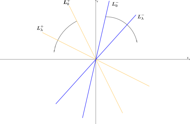
(a) In this case $\lambda\mapsto L_{\lambda}^{+}$ is approaching the $x$-axis in the counter-clockwise direction whilst $\lambda\mapsto L_{\lambda}^{-}$ is approaching the $x$-axis clockwise direction and so, no coincidence times on $[0,\widehat{\lambda}]$.

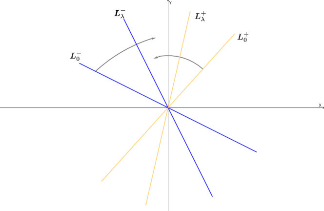
(b) In this case $\lambda\mapsto L_{\lambda}^{+}$ is approaching the $x$-axis in the counter-clockwise direction whilst $\lambda\mapsto L_{\lambda}^{-}$ is approaching the $x$-axis clockwise direction and so, only one coincidence time on $[0,\widehat{\lambda}]$.

Then $E^{s}_{\lambda}(+\infty)$ represents the straight line $L_{\lambda}^{+}$ through the origin with a slope (with respect to the $y$ axis) of $Q_{+}-\sqrt{P_{+}(R_{+}+\lambda)}$ and $E^{u}_{\lambda}(-\infty)$ represents the straight line $L_{\lambda}^{-}$ through the origin with slope (with respect to the $y$ axis) of $Q_{-}+\sqrt{P_{-}(R_{-}+\lambda)}$. It is immediate to observe that $L^{+}_{\lambda}$ (resp. $L^{-}_{\lambda}$) approaches the $x$ -axis in the counterclockwise (resp. clockwise) direction as $\lambda$ increases to $\infty$ respectively. So $\operatorname{\iota^{\scriptscriptstyle{\mathrm{CLM}}}}\left(E^{s}_{\lambda}(+\infty),E^{u}_{\lambda}(-\infty),\lambda\in[0,\widehat{\lambda}]\right)$ equal to the total number of counting the coincidence times (overlapping times) between $L_{\lambda}^{+}$ and $L_{\lambda}^{-}$ as $\lambda$ increases from $0$ up to $\widehat{\lambda}$. We consider the following two cases.

• Case 1 (depicted in Figure 1(a)). If condition (H2) holds, then we get that $\sqrt{P_{\pm}R_{\pm}}\mp Q_{\pm}>0$ and so the line $L^{+}_{0}$ (resp. $L_{0}^{-}$) lies on the left (resp. right) half-plane bounded by the $y$-axis. By the above discussion we get that the coincidence times between $L^{+}_{\lambda}$ and $L^{-}_{\lambda}$ is 0, and then $\operatorname{\iota^{\scriptscriptstyle{\mathrm{CLM}}}}\left(E^{s}_{\lambda}(+\infty),E^{u}_{\lambda}(-\infty),\lambda\in[0,\widehat{\lambda}]\right)=0$. So, by the Morse index formula, we get $\operatorname{m^{--}}(u)=\iota(u).$

• Case 2 (depicted in Figure 1(b)). If $\sqrt{P_{\pm}R_{\pm}}\mp Q_{\pm}<0$ , $Q_{+}>0$ and $Q_{-}<0$, it is easy to see that the line $L^{+}_{0}$ (resp. $L_{0}^{-}$) lies on the right (resp. left) half-plane bounded by the $y$-axis. By the above discussion we get that the coincidence times between $L^{+}_{\lambda}$ and $L^{-}_{\lambda}$ is 1 since $L^{+}_{\lambda}$ and $L^{-}_{\lambda}$ will overlap just once as $\lambda\to+\infty$. Thus, we get $\operatorname{\iota^{\scriptscriptstyle{\mathrm{CLM}}}}\left(E^{s}_{\lambda}(+\infty),E^{u}_{\lambda}(-\infty),\lambda\in[0,\widehat{\lambda}]\right)=-1$ and $\operatorname{m^{--}}(u)=\iota(u)+1$.

Notation 1.12.

We let $L_{0}\in L(n)$ be a Lagrangian subspace and we denote by $\operatorname{m^{--}}(u),\ \operatorname{m^{--}}(u,L_{0},+)$ and $\operatorname{m^{--}}(u,L_{0},-)$ the Morse indices of the operators $\mathscr{A}$, $\mathscr{A}^{-}$ and $\mathscr{A}^{+}$respectively on their domains $E,E^{-}_{L_{0}}$ and $E^{+}_{L_{0}}$. The next result provides some spectral flow formulas in the case of future and past half-clinic orbits of Legendre convex systems under very general self-adjoint boundary condition.

The following result of this paper provides a spectral flow formula for half-clinic orbits in the case of Legendre convex Lagrangian functions, with respect to a general self-adjoint boundary condition.

Theorem 4.

Let $L$ be the Lagrangian and let $u$ be a solution either of Equation (1.2) or Equation (1.3). If condition (F2)& (H1) are fulfilled, then we get

• (future half-clinic case)

  $$\operatorname{m^{--}}(u,L_{0},+)=\operatorname{\iota}^{+}_{L_{0}}(u)+\iota\left(L_{D},L_{0};E^{s}(+\infty)\right).$$ (1.28)

• (past half-clinic case)

  $$\operatorname{m^{--}}(u,L_{0},-)=\operatorname{\iota}^{-}_{L_{0}}(u)+\iota\left(E^{u}(-\infty),L_{0};L_{D}\right).$$ (1.29)

As direct consequence of Theorem 4, we provide a characterization of the difference of the Morse indices of a half-clinic orbit for a Legendre convex Lagrangian system, in terms of the triple index and of the relative position of the Lagrangian subspaces $L_{0},L_{D}$ and finally $E^{s}(0)$ or $E^{u}(0)$.

Corollary 1.13.

Let $u$ be a solution of the boundary value problem given in Equation (1.2) or in Equation (1.3). If condition (F2) & (H1) are fulfilled, then we get

• (future half-clinic orbit)

  $$\operatorname{m^{--}}(u,L_{0},+)-\operatorname{m^{--}}(u,L_{D},+)=\iota\big{(}L_{D},L_{0},E^{s}(0)\big{)}$$ (1.30)

• (past half-clinic orbit)

  $$\operatorname{m^{--}}(u,L_{0},-)-\operatorname{m^{--}}(u,L_{D},-)=\iota\left(E^{u}(0),L_{0};L_{D}\right)$$ (1.31)

  .

2 Fredholmness and hyperbolicity

The aim of this section is twofold. In Subsection 2.1, we provide some sufficient condition on the hyperbolicity of the limiting Hamiltonian systems which is a crucial property for establishing the Fredholmness of the Sturm-Liouville operators defined both on the line and on the half-line. All of these conditions directly involve either the coefficients appearing in the Sturm-Liouville operator or the bounds given in condition (F1), (F2), (H1) and (H2). Subsection 2.2 is functional analytic oriented and we provide the full details about the Fredholmness of the Sturm-Liouville operators both on the line and on the half-line as well as for the (first order) Hamiltonian differential operators induced. In order to consider all boundary conditions at once the maximal and minimal operators play a crucial role throughout this subsection.

2.1 About the hyperbolicity of the limiting matrices

The aim of this section is to prove some useful hyperbolicity condition for the limiting matrices in terms of the coefficients of the Sturm-Liouville operators $\mathscr{A}$ and $\mathscr{A}^{\pm}$ as well as in terms of the bounds appearing in condition (F1).

The first useful result is a characterization of the hyperbolicity of the matrix $JB$ for

$$B=\begin{bmatrix}P^{-1}&-P^{-1}Q\\ -{Q}^{\mathsf{T}}P^{-1}&{Q}^{\mathsf{T}}P^{-1}Q-R\end{bmatrix}$$ (2.1)

in terms of a non-vanishing determinant of a suitable matrix.

Lemma 2.1.

Assume that $P$ invertible, then $JB$ is hyperbolic if and only if

$$\det\left[a^{2}P+ia({Q}^{\mathsf{T}}-Q)+R\right]\neq 0\quad\textrm{ for }a\in\mathbb{R}.$$

Proof.

$JB$ is hyperbolic if and only if $\det(JB+iaI)\neq 0$ for all $a\in\mathbb{R}$. By a strightforward calculation, we get

$$\det(JB+iaI)=\det(B-iaJ)=\det\begin{bmatrix}P^{-1}&-P^{-1}Q+iaI\\ -{Q}^{\mathsf{T}}P^{-1}-iaI&{Q}^{\mathsf{T}}P^{-1}Q-R\end{bmatrix}\\ =\det\begin{bmatrix}I&0\\ [{Q}^{\mathsf{T}}P^{-1}+iaI]P&I\end{bmatrix}\begin{bmatrix}P^{-1}&-P^{-1}Q+iaI\\ -{Q}^{\mathsf{T}}P^{-1}-iaI&{Q}^{\mathsf{T}}P^{-1}Q-R\end{bmatrix}\\ =\det\begin{bmatrix}P^{-1}&-P^{-1}Q+iaI\\ 0&-iaQ+ia{Q}^{\mathsf{T}}-a^{2}P-R\end{bmatrix}\\ =\det P^{-1}\det\big{[}-a^{2}P-R-ia[Q-{Q}^{\mathsf{T}}]\big{]}.$$ (2.2)

Thus we get that $\det(JB+iaI)\neq 0$ iff $\det\big{[}-a^{2}P-R-ia[Q-{Q}^{\mathsf{T}}]\big{]}$ and this concludes the proof. ∎

The following result will be useful later and gives a sufficient condition on the hyperbolicity of $JB$ in terms of a symmetric matrix constructed through the coefficient matrices of the Sturm-Liouville operators.

Corollary 2.2.

If $\begin{bmatrix}P&Q\\ {Q}^{\mathsf{T}}&R\end{bmatrix}$ are positive definite then $JB$ is hyperbolic.

Proof.

We start by observing that $a^{2}P+ia({Q}^{\mathsf{T}}-Q)+R=\begin{bmatrix}iaI&I\end{bmatrix}\begin{bmatrix}P&Q\\ {Q}^{\mathsf{T}}&R\end{bmatrix}\begin{bmatrix}-iaI\\ I\end{bmatrix}$. Since, by assumption, the matrix $\begin{bmatrix}P&Q\\ {Q}^{\mathsf{T}}&R\end{bmatrix}$ is positive definite, then the matrix $a^{2}P+ia({Q}^{\mathsf{T}}-Q)+R$ is positive definite, too and in particular its determinant is non vanishing. Then the corollary follows direct by Lemma 2.1. ∎

The following result gives a sufficient condition about the hyperbolicity of a special path of Hamiltonian matrices if the starting point matrix is hyperbolic.

Lemma 2.3.

Let $R_{\lambda}=R+\lambda I$ and let $JB_{\lambda}$ where $B_{\lambda}$ is obtained by replacing $R$ with $R_{\lambda}$ in Equation (2.1). We assume condition (F2) holds and that $JB_{\lambda}$ is hyperbolic for $\lambda=0$. Then we get that $JB_{\lambda}$ is hyperbolic for all $\lambda\in\mathbb{R}^{+}$.

Proof.

We start by introducing the following one parameter family of functions defined as following $f_{\lambda}(a)\coloneqq a^{2}P+ia({Q}^{\mathsf{T}}-Q)+R+\lambda I$. By assumption and by taking into account Lemma 2.1 we infer that $f_{0}(a)\neq 0$ for all $a\in\mathbb{R}$. If $a$ is sufficiently large, then $f_{0}(a)$ is positive definite, so without leading in generalities, we can assume that $f_{0}(a)$ is positive definite for all $a\in\mathbb{R}$.

Therefore, for every $\lambda>0$, we have that $f_{\lambda}(a)=f_{0}(a)+\lambda I>f_{0}(a)$ or which is the same tha the matrix $f_{\lambda}(a)$ is positive definite for all $(\lambda,a)\in\mathbb{R}^{+}\times\mathbb{R}$. By using once again Lemma 2.1, the thesis directly follows. ∎

Let $R_{\lambda}=R+\lambda I$ and we observe that, as direct consequence of the bounds given in condition (F1), that the following result holds.

Corollary 2.4.

Assume that $P,Q,R$ satisfy condition (F2) and let $R_{\lambda}=R+\lambda I$. Then, for $\lambda>C_{2}^{2}/C_{1}+C_{3}$, the associated matrix $JB_{\lambda}$ is hyperbolic.

Proof.

By invoking Corollary 2.2, we need to prove that the matrix $\begin{bmatrix}P&Q\\ {Q}^{\mathsf{T}}&R_{\lambda}\end{bmatrix}$ is positive definite. So, it is enough to observe that

$$\begin{bmatrix}x^{T}&y^{T}\end{bmatrix}\begin{bmatrix}P&Q\\ {Q}^{\mathsf{T}}&R_{\lambda}\end{bmatrix}\begin{bmatrix}x\\ y\end{bmatrix}=(Px,x)+(Qy,x)+({Q}^{\mathsf{T}}x,y)+(R_{\lambda}y,y)\\ \geq C_{1}|x|^{2}-2C_{2}|x||y|-C_{3}|y|^{2}+\lambda|y|^{2}\geqslant C_{1}(|x|-C_{2}/C_{1}|y|)^{2}+(-C_{3}-C_{2}^{2}/C_{1}+\lambda)|y|^{2}.$$ (2.3)

This inequality implies that $\begin{bmatrix}P&Q\\ {Q}^{\mathsf{T}}&R_{\lambda}\end{bmatrix}$ is positive definite for every $\lambda>C_{2}^{2}/C_{1}+C_{3}$. ∎

A similar result holds by replacing the path $\lambda\mapsto R+\lambda I$ with the following one $\lambda\mapsto R_{\lambda}\coloneqq\lambda P$ which is very useful in very many situations.

Corollary 2.5.

Assume that $P$ invertible and let $R_{\lambda}=\lambda P$. Then, there exists $\widehat{\lambda}>0$ such that, for every $\lambda>\widehat{\lambda}$ the matrix $JB_{\lambda}$ is hyperbolic.

Proof.

We start by observing that

$$a^{2}P+ia[{Q}^{\mathsf{T}}-Q]+R_{\lambda}=[a^{2}+\lambda]P+ia[{Q}^{\mathsf{T}}-Q]=P[a^{2}+\lambda]\left[I+\dfrac{ia}{a^{2}+\lambda}P^{-1}[{Q}^{\mathsf{T}}-Q]\right].\\$$ (2.4)

For positive $\lambda$ we get $\left|\dfrac{a}{a^{2}+\lambda}\right|\leqslant\left|\dfrac{1}{2\sqrt{\lambda}}\right|$. So, there exists $\widehat{\lambda}>0$ such that for each $\lambda>\widehat{\lambda}$, we get

$$\left\|\dfrac{ia}{a^{2}+\lambda}P^{-1}({Q}^{\mathsf{T}}-Q)\right\|<1.$$

This inequality directly implies that the matrix $a^{2}P+ia({Q}^{\mathsf{T}}-Q)+R_{\lambda}$ is invertible for every $\lambda>\widehat{\lambda}$. By invoking Lemma 2.1, we get the thesis. ∎

2.2 Results from functional analysis

We start by recalling a classical abstract result (consequence of the closed graph theorem) useful for comparing operators Sturm-Liouville and Hamiltonian operators on different domains.

Lemma 2.6.

[Kat80, Chapter IV, Theorem 5.2 & Problem 5.7] Let $X,\ Y$ be two Banach spaces and consider a closed linear operator $L:\operatorname{dom}L\subset X\to Y$ with a dense domain $\operatorname{dom}L$. Assume that $\operatorname{codim}L<+\infty$, then we have that $\mathrm{rge}\,L$ is closed in $Y$.

Remark 2.7.

Before proceeding further we pause by observing that all of the results of this paragraph involving the operators on the positive half-line holds for the differential operators defined on the negative half-line, as well.

By using Lemma 2.6 the following characterization fore the Fredholmness of the operator $\mathscr{A}^{+}$ (and $\mathscr{A}^{-}$ as already observed).

Lemma 2.8.

Under the above notation, we get that the operator $\mathscr{A}^{+}$ is Fredholm if and only if the operator $\mathscr{A}_{m}^{+}$ is Fredholm.

Proof.

We start to consider the (maximal) Sturm-Liouville operator $\mathscr{A}_{M}^{+}$ on $W^{2,2}$; i.e.

$$\mathscr{A}_{M}^{+}\coloneqq-\dfrac{d}{dt}\left(P(t)\dfrac{d}{dt}+Q(t)\right)+{Q}^{\mathsf{T}}(t)\dfrac{d}{dt}+R(t):W^{2,2}(\mathbb{R}^{+},\mathbb{R}^{n})\subset L^{2}(\mathbb{R}^{+};\mathbb{R}^{n})\to L^{2}(\mathbb{R}^{+};\mathbb{R}^{n}).$$

Since $\mathscr{A}_{M}$ and $\mathscr{A}_{m}$ are conjugated with respect to the $L^{2}$ scalar product, so $\mathscr{A}_{m}$ is a Fredholm operator if and only if $\mathscr{A}_{M}$ is a Fredholm operator. Moreover the following inclusion holds

$$\ker\left(\mathscr{A}^{+}_{m}\right)\subset\ker\left(\mathscr{A}^{+}\right)\subset\ker\left(\mathscr{A}^{+}_{M}\right)\textrm{ and }\mathrm{rge}\,\left(\mathscr{A}^{+}_{m}\right)\subset\mathrm{rge}\,\left(\mathscr{A}^{+}\right)\subset\mathrm{rge}\,\left(\mathscr{A}^{+}_{M}\right).$$

$(\Leftarrow)$ We assume that $\mathscr{A}_{m}^{+}$ is Fredholm and we want to prove that $\mathscr{A}^{+}$ is Fredholm too. For, we start by observing that $\operatorname{codim}\left(\mathscr{A}^{+}\right)\leqslant\operatorname{codim}\left(\mathscr{A}^{+}_{m}\right)<+\infty$. Being $\mathscr{A}^{+}$ a closed operator and by using Lemma 2.6 and since $\operatorname{codim}\left(\mathscr{A}^{+}\right)<+\infty$, we get that $\mathrm{rge}\,\left(\mathscr{A}^{+}\right)$ is closed. So we have that $\mathscr{A}^{+}$ is a Fredholm operator.

$(\Rightarrow)$. The converse implication goes through the same arguments and is left to the reader. This concludes the proof. ∎

By using the same arguments, the following result holds.

Lemma 2.9.

The operator $\mathscr{F}^{+}$ is Fredholm if and only if the operator $\mathscr{F}_{m}^{+}$ is Fredholm.

A couple of technical lemmas for getting the characterization of the Fredhomness of the Sturm-Liouville operators in terms of the Fredholmness of the Hamiltonian operators, are in order.

• The first one is about the non-degeneracy in $W_{0}^{1,2}(\mathbb{R}^{+},\mathbb{R}^{2n})$ of a one parameter family of Hamiltonian operators on the half-line

• The second is about the hyperbolicity of the limiting Hamiltonian systems

Remark 2.10.

Both these results are useful for proving the closedness of the image of the minimal Hamiltonian differential operator assuming the closedness of the image of the minimal Sturm-Liouville operator. The other way around is almost straightforward.

So, for each $s\in\mathbb{R}$, we let $\mathscr{F}^{+}_{0,s}:L^{2}(\mathbb{R}^{+},\mathbb{R}^{2n})\rightarrow L^{2}(\mathbb{R}^{+},\mathbb{R}^{2n})$ be the operator defined by

$${\mathscr{F}^{+}_{0,s}}\coloneqq-J\dfrac{d}{dt}-B_{s}(t)$$ (2.5)

where $\operatorname{dom}\mathscr{F}^{+}_{0,s}=\left\{z\in W^{1,2}(\mathbb{R}^{+},\mathbb{R}^{2n})|z(0)=0\right\}=W_{0}^{1,2}(\mathbb{R}^{+},\mathbb{R}^{2n})$ and

$$B_{s}(t)=\begin{bmatrix}P^{-1}(t)&-P^{-1}(t)Q(t)\\ -{Q}^{\mathsf{T}}(t)P^{-1}&{Q}^{\mathsf{T}}(t)P^{-1}(t)Q(t)-sP(t)\end{bmatrix}.$$

We let $B^{+}_{s}=\lim\limits_{t\to+\infty}B_{s}(t)$ uniformly with respect to $s$.

Lemma 2.11.

The operator $\mathscr{F}^{+}_{0,s}$ is non-degenerate for every $s\in\mathbb{R}$.

Proof.

We consider the following Hamiltonian system:

$$\begin{cases}\dot{z}(t)=JB_{s}(t)z(t)\qquad t\in\mathbb{R}^{+}\\ z(0)=0\end{cases}$$ (2.6)

and we observe that that $\ker\mathscr{F}_{0,s}^{+}$ consists of all solutions of Equation (2.6). By the uniqueness theorem for odes, the Hamiltonian system given in quation (2.6) has only the trivial solution. This implies that $\mathscr{F}^{+}_{0,s}$ is non-degenerate for all $s\in\mathbb{R}$. ∎

Lemma 2.12.

There exists $\widehat{s}$ such that $JB^{+}_{s}$ is hyperbolic for every $s\geqslant\widehat{s}$.

Proof.

This result is a direct consequence of Corollary 2.5. ∎

Remark 2.13.

The idea for introducing the one parameter $s$-dependent family of Hamiltonian operators $\mathscr{F}^{+}_{0,s}$ is in order to get a Fredholm operator on $W_{0}^{1,2}$ only by modifying the zero order term and to help in the proof of Proposition 2.14.

The following result gives a characterization of the Fredholmness of the operator $\mathscr{A}_{m}$ (resp. $\mathscr{A}^{\pm}_{m}$) in terms of $\mathscr{F}_{m}$ (resp. $\mathscr{F}_{m}^{\pm}$).

Proposition 2.14.

The operator $\mathscr{A}_{m}^{+}:W_{0}^{2,2}\subset L^{2}(\mathbb{R}^{+};\mathbb{R}^{n})\to L^{2}(\mathbb{R}^{+};\mathbb{R}^{n})$ is Fredholm if and only if the operator

$$\mathscr{F}_{m}^{+}\coloneqq-J\dfrac{d}{dt}-B(t):W_{0}^{1,2}(\mathbb{R}^{+};\mathbb{R}^{2n})\subset L^{2}(\mathbb{R}^{+};\mathbb{R}^{2n})\to L^{2}(\mathbb{R}^{+};\mathbb{R}^{2n})$$

is Fredholm. Furthermore their Fredholm indices both coincide.

Proof.

We start by observing that $\mathscr{F}_{m}^{+}$ and $\mathscr{A}_{m}^{+}$ are both symmetric operators whose adjoint are respectively $\mathscr{F}_{M}^{+}$ and $\mathscr{A}_{M}^{+}$. Thus, we get $\ker(\mathscr{F}_{M}^{+})=\mathrm{rge}\,(\mathscr{F}_{m}^{+})^{\perp}$ and $\ker(\mathscr{A}_{M}^{+})=\mathrm{rge}\,(\mathscr{A}_{m}^{+})^{\perp}$. Moreover, it is well-known that $\dim\ker(\mathscr{A}_{M}^{+})=\dim\ker(\mathscr{F}_{M}^{+})\leq 2n$ and $\dim\ker(\mathscr{A}_{m}^{+})=\dim\ker(\mathscr{F}_{m}^{+})=0$. So, in order to conclude the proof of the first claim, we only need to prove that

• $\mathrm{rge}\,(\mathscr{A}_{m}^{+})$ is closed if and only if $\mathrm{rge}\,(\mathscr{F}_{m}^{+})$ is closed.

Let us consider the closed subspaces

$$H_{1}\coloneqq\Set{{(v,0)}^{\mathsf{T}}}{v\in L^{2}(\mathbb{R}^{+},\mathbb{R}^{n})}\quad\textrm{ and }\quad H_{2}\coloneqq\Set{{(0,u)}^{\mathsf{T}}}{u\in L^{2}(\mathbb{R}^{+},\mathbb{R}^{n})}$$

and we observe that $L^{2}=H_{1}\oplus H_{2}$.

First claim.

The following implication holds

$$\mathrm{rge}\,(\mathscr{F}_{m}^{+})\textrm{ is closed }\quad\Rightarrow\quad\mathrm{rge}\,(\mathscr{A}_{m}^{+})\textrm{ is closed }$$

A straightforward computation shows that

$$\mathscr{F}_{m}^{+}\begin{bmatrix}y\\ x\end{bmatrix} =\begin{bmatrix}0\\ h\end{bmatrix}\Longleftrightarrow y=P\dot{x}+Qx\text{\ and\ }\mathscr{A}^{+}_{m}x=h.$$ (2.7)

Equation (2.7) implies that

$$h\in\mathrm{rge}\,(\mathscr{A}_{m}^{+})\Longleftrightarrow\begin{bmatrix}0\\ h\end{bmatrix}\in\mathrm{rge}\,(\mathscr{F}_{m}^{+}).$$ (2.8)

It follows that $H_{2}\cap\mathrm{rge}\,(\mathscr{F}_{m}^{+})$ is isomorphic to $\mathrm{rge}\,(\mathscr{A}^{+}_{m})$ . So, if $\mathrm{rge}\,(\mathscr{F}_{m}^{+})$ is closed, then $\mathrm{rge}\,(\mathscr{A}_{m}^{+})$ is closed as well.

Second claim.

We now show that

$$\mathrm{rge}\,(\mathscr{A}_{m}^{+})\textrm{ is closed }\quad\Rightarrow\quad\mathrm{rge}\,(\mathscr{F}_{m}^{+})\textrm{ is closed }$$

We assume that $\mathrm{rge}\,(\mathscr{A}_{m}^{+})$ is closed. To conclude, it is enough to show that $H_{2}\cap\mathrm{rge}\,\mathscr{F}_{m}^{+}$ is closed in $L^{2}(\mathbb{R},\mathbb{R}^{2n})$. Let now $s>\widehat{s}$ (where $\widehat{s}$ is given in Lemma 2.12). By Lemma 2.11 and Lemma 2.12, we get that $\mathscr{F}^{+}_{0,s}$ is a Fredholm operator (being invertible on its domain) and $\ker\left(\mathscr{F}^{+}_{0,s}\right)=\{0\}$, as well. By the closed graph theorem we conclude that $\mathscr{F}^{+}_{0,s}$ has a bounded inverse on $\mathrm{rge}\,\mathscr{F}^{+}_{0,s}$ . Let $f\in\mathrm{rge}\,\mathscr{F}_{0,s}^{+}$. Then, we have

$$f-\mathscr{F}_{m}^{+}\left(\mathscr{F}_{0,s}^{+}\right)^{-1}f=\left(\mathscr{F}^{+}_{0,s}-\mathscr{F}_{m}^{+}\right)\left(\mathscr{F}_{0,s}^{+}\right)^{-1}f=\begin{bmatrix}0&0\\ 0&R_{+}-sP_{+}\end{bmatrix}\left(\mathscr{F}_{0,s}^{+}\right)^{-1}f\in H_{2}.$$ (2.9)

Let $T=I-\mathscr{F}_{m}^{+}\left(\mathscr{F}_{0,s}^{+}\right)^{-1}$. Then $T$ is a continuous operator from $\mathrm{rge}\,\mathscr{F}^{+}_{0,s}$ to $H_{2}$ and $Tf\in\mathrm{rge}\,\mathscr{F}_{m}^{+}$ if and only if $f\in\mathrm{rge}\,\mathscr{F}_{m}^{+}$. It follows that

$$\mathrm{rge}\,\mathscr{F}^{+}_{0,s}\cap\mathrm{rge}\,\mathscr{F}^{+}_{m}=T^{-1}(H_{2}\cap\mathrm{rge}\,\mathscr{F}^{+}_{m}).$$ (2.10)

So $\mathrm{rge}\,\mathscr{F}^{+}_{0,s}\cap\mathrm{rge}\,\mathscr{F}^{+}_{m}$ is closed. Let $X=L^{2}(\mathbb{R},\mathbb{R}^{2n})$. We have

$$\mathrm{rge}\,\mathscr{F}^{+}_{m}/(\mathrm{rge}\,\mathscr{F}^{+}_{0,s}\cap\mathrm{rge}\,\mathscr{F}^{+}_{m})\cong(\mathrm{rge}\,\mathscr{F}^{+}_{0,s}+\mathrm{rge}\,\mathscr{F}^{+}_{m})/\mathrm{rge}\,\mathscr{F}^{+}_{0,s}$$ (2.11)

Note that $\dim(\mathrm{rge}\,\mathscr{F}^{+}_{0,s}+\mathrm{rge}\,\mathscr{F}^{+}_{m})/\mathrm{rge}\,\mathscr{F}^{+}_{0,s}\leq\text{codim}\mathscr{F}_{0,s}^{+}$. So $\dim(\mathrm{rge}\,\mathscr{F}^{+}_{m}/(\mathrm{rge}\,\mathscr{F}^{+}_{0,s}\cap\mathrm{rge}\,\mathscr{F}^{+}_{m}))<\infty$. Then $\mathrm{rge}\,\mathscr{F}^{+}_{m}$ is a direct sum of $\mathrm{rge}\,\mathscr{F}^{+}_{0,s}\cap\mathrm{rge}\,\mathscr{F}^{+}_{m}$ with a finite dimensional space. So $\mathrm{rge}\,\mathscr{F}^{+}_{m}$ is closed since $\mathrm{rge}\,\mathscr{F}^{+}_{0,s}\cap\mathrm{rge}\,\mathscr{F}^{+}_{m}$ is closed.

The second claim is a straightforward consequence of the previous equalities. By these the result follows. ∎ We let $B_{+}\coloneqq\begin{bmatrix}P^{-1}_{+}&-P^{-1}_{+}Q_{+}\\ -{Q}^{\mathsf{T}}P^{-1}_{+}&{Q}^{\mathsf{T}}_{+}P^{-1}_{+}Q_{+}-R_{+}\end{bmatrix}$ where $P_{+},Q_{+},R_{+}$ are the matrices appearing in condition (H2) and we define the following operators

$$\widehat{\mathscr{F}^{+}} \coloneqq-J\frac{\operatorname{d}}{\operatorname{d}t}-B_{+}:W^{+}_{L_{0}}(\mathbb{R}^{+},\mathbb{R}^{2n})\subset L^{2}\left(\mathbb{R}^{+},\mathbb{R}^{2n}\right)\to L^{2}\left(\mathbb{R}^{+},\mathbb{R}^{2n}\right)$$

$$\widehat{\mathscr{F}_{m}^{+}} \coloneqq-J\frac{\operatorname{d}}{\operatorname{d}t}-B_{+}:W_{0}^{1,2}(\mathbb{R}^{+},\mathbb{R}^{2n})\subset L^{2}\left(\mathbb{R}^{+},\mathbb{R}^{2n}\right)\to L^{2}\left(\mathbb{R}^{+},\mathbb{R}^{2n}\right)$$

$$\widehat{\mathscr{F}_{M}^{+}} \coloneqq-J\frac{\operatorname{d}}{\operatorname{d}t}-B_{+}:W^{1,2}(\mathbb{R}^{+},\mathbb{R}^{2n})\subset L^{2}\left(\mathbb{R}^{+},\mathbb{R}^{2n}\right)\to L^{2}\left(\mathbb{R}^{+},\mathbb{R}^{2n}\right)$$ (2.12)

Lemma 2.15.

The operator $\mathscr{F}^{+}$ defined in Equation (1.12), namely

$$\mathscr{F}^{+}=-J\frac{\operatorname{d}}{\operatorname{d}t}-B(t):W^{+}_{L_{0}}(\mathbb{R}^{+},\mathbb{R}^{2n})\subset L^{2}\left(\mathbb{R}^{+},\mathbb{R}^{2n}\right)\to L^{2}\left(\mathbb{R}^{+},\mathbb{R}^{2n}\right)$$

is a relatively compact perturbation of the operator $\widehat{\mathscr{F}^{+}}$ given in Equation (2.2).

Proof.

To prove that $\mathscr{F}^{+}=-J\frac{\operatorname{d}}{\operatorname{d}t}-B(t)$ is a relatively compact perturbation of the operator $\widehat{\mathscr{F}}$, we fix $\lambda$ in the resolvent set of $\widehat{\mathscr{F}^{+}}$, and we need to prove that the operator

$$L_{\lambda}=\left(\mathscr{F}^{+}-\widehat{\mathscr{F}^{+}}\right)\circ\left(\widehat{\mathscr{F}^{+}}-\lambda I\right)^{-1}:L^{2}\left(\mathbb{R}^{+},\mathbb{R}^{2n}\right)\to L^{2}\left(\mathbb{R}^{+},\mathbb{R}^{2n}\right)$$

is compact.

Define a sequence $\{\chi_{k}\}$ of $C^{\infty}$ function on $\mathbb{R}^{+}$ which satisfy $\sup\limits_{t\in\mathbb{R}^{+}}|\chi(t)|\leqslant 1$, $\sup\limits_{t\in\mathbb{R}^{+}}|\chi^{\prime}(t)|\leqslant 1$ and

$$\chi_{k}(t)=\begin{cases}1,\ \text{if }t\in[0,k-1],\\ 0,\ \text{if }t\in[k,+\infty).\end{cases}$$

We define a bounded multiplication operator through the action of $\chi_{k}$

$$\alpha_{k}:L^{2}(\mathbb{R}^{+},\mathbb{R}^{2n})\ni x\longmapsto\chi_{k}x\in L^{2}(\mathbb{R}^{+},\mathbb{R}^{2n})$$

and let us consider the following operators defined by

$$L_{k,\lambda}=\left(\mathscr{F}^{+}-\widehat{\mathscr{F}^{+}}\right)\circ\alpha_{k}\circ\left(\widehat{\mathscr{F}^{+}}-\lambda I\right)^{-1}:L^{2}\left(\mathbb{R}^{+},\mathbb{R}^{2n}\right)\to L^{2}\left(\mathbb{R}^{+},\mathbb{R}^{2n}\right).$$

We observe that

$$\left(\mathscr{F}^{+}-\widehat{\mathscr{F}^{+}}\right)(\alpha_{k}-I)x=(B_{+}-B(t))(\chi_{k}(t)-1)x(t)$$

and $\lim_{k\to\infty}(B_{+}-B(t))(\chi_{k}(t)-1)=0$ uniformly with respect to $t$.

So, we get that $\left(\mathscr{F}^{+}-\widehat{\mathscr{F}^{+}}\right)(\alpha_{k}-I)$ converge to $0$ in the operator norm topology and this, in particular, implies that the operator $L_{k,\lambda}\to L_{\lambda}$ in the operator norm. Thus, in order to conclude, we need to prove that the operator $L_{k,\lambda}$ is compact for all $k$ (being, in this case, the set of compact operators, a closed ideal of the linear bounded operators onto $L^{2}$). We observe that the operator

$$\left(\widehat{\mathscr{F}^{+}}-\lambda I\right)^{-1}:L^{2}\left(\mathbb{R}^{+},\mathbb{R}^{2n}\right)\to W^{1,2}(\mathbb{R}^{+},\mathbb{R}^{2n})$$

is bounded. Since $\chi_{k}(t)=0$ for all $t\geqslant k$ and $\sup\limits_{t\in\mathbb{R}^{+}}|\chi(t)|\leqslant 1$, $\alpha_{k}:x\to\chi_{k}x$ is a bounded operator from $W^{1,2}(\mathbb{R}^{+},\mathbb{R}^{2n})$ to $W^{1,2}([0,k],\mathbb{R}^{2n})$. By the Sobolev embedding theorem, we get that $W^{1,2}\left([0,k],\mathbb{R}^{2n}\right)$ into $L^{2}\left([0,k],\mathbb{R}^{2n}\right)$ is compact. So $\alpha_{k}\circ\left(\widehat{\mathscr{F}^{+}}-\lambda I\right)^{-1}$ is a compact operator from $L^{2}(\mathbb{R}^{+},\mathbb{R}^{2n})$ to $L^{2}(\mathbb{R}^{+},\mathbb{R}^{2n})$. Since $\mathscr{F}^{+}-\widehat{\mathscr{F}^{+}}$ is bounded, then the operator $L_{\lambda,k}$ is compact. This concludes the proof. ∎

Lemma 2.16.

The operator $\widehat{\mathscr{F}_{M}^{+}}$ defined by Equation (2.2) is Fredholm if and only if the matrix $JB_{+}$ is hyperbolic. If the operator $\widehat{\mathscr{F}_{M}^{+}}$ is Fredholm, then its Fredholm index is equal to the dimension of the negative spectral space of the matrix $JB_{+}$, e.g. $\operatorname{ind}\widehat{\mathscr{F}_{M}^{+}}=\dim V^{-}(JB_{+})$.

Proof.

By [RS05b, Theorem 2.3] we get that the constant coefficients differential operator given by

$$\mathscr{B}\coloneqq\dfrac{\operatorname{d}}{\operatorname{d}t}-JB_{+},$$ (2.13)

where $\operatorname{dom}\mathscr{B}=W^{1,2}\left(\mathbb{R}^{+},\mathbb{R}^{2n}\right)$ is Fredholm if and only if the matrix $JB_{+}$ is hyperbolic. Moreover, if the operator ${\mathscr{B}}$ is Fredholm, then the following equality holds, $\operatorname{ind}\mathscr{B}=\dim V^{-}(JB_{+})$.

It is straightforward to check that $\mathrm{rge}\,\left(\widehat{\mathscr{F}_{M}^{+}}\right)=-J\mathrm{rge}\,\left(\mathscr{B}\right)$, which implies that $\text{codim}\left(\widehat{\mathscr{F}_{M}^{+}}\right)=\text{codim}\left({\mathscr{B}}\right)$ and $\ker\left(\widehat{\mathscr{F}_{M}^{+}}\right)=\ker\left(\mathscr{B}\right)$. The thesis readily follows by Lemma 2.6 and [RS05b, Lemma 2.1]. ∎

Corollary 2.17.

The operator $\widehat{\mathscr{F}_{m}^{+}}$ defined in Equation (2.2) is Fredholm if and only if the matrix $JB_{+}$ is hyperbolic.

Proof.

We recall that $\widehat{\mathscr{F}_{m}^{+}}$ and $\widehat{\mathscr{F}_{M}^{+}}$ are conjugated. The thesis follows by this remark and by using Lemma 2.16. ∎

3 Proofs of Theorem 1 and Theorem 2

As direct consequence of the results proved in Subsection 2.2, we are in position to prove Theorem 1.

3.1 Proof of Theorem 1

Let us start with the proof of the Fredholmness of $\mathscr{A}^{+}$.

Theorem 3.1.

The operator $\mathscr{A}^{+}$ defined in Equation (1.8) is Fredholm if and only if $JB_{+}$ is hyperbolic.

Proof.

From [Kat80, Chapter IV, Theorem 5.35], Lemma 2.15 and Corollary 2.17, we get that $\mathscr{F}^{+}_{m}$ is Fredholm if and only if the matrix $JB_{+}$ is hyperbolic. The conclusion now follows by invoking Lemma 2.14 and Lemma  2.8. This concludes the proof ∎

A completely analogous argument leads to the same conclusion for the operator $\mathscr{A}^{-}$ defined by Equation (1.8). (Cfr. Remark 2.7).

Theorem 3.2.

The operator $\mathscr{A}^{-}$ defined in Equation (1.8) is Fredholm if and only if $JB_{-}$ is hyperbolic.

We define the following operator $\widetilde{\mathscr{A}_{M}}=\left(\mathscr{A}_{M}^{-},\mathscr{A}_{M}^{+}\right)$ as follows

$$\widetilde{\mathscr{A}_{M}}:\operatorname{dom}\mathscr{A}_{M}^{-}\oplus\operatorname{dom}\mathscr{A}_{M}^{+}\subset L^{2}\left(\mathbb{R}^{-},\mathbb{R}^{n}\right)\oplus L^{2}\left(\mathbb{R}^{+},\mathbb{R}^{n}\right)\to L^{2}\left(\mathbb{R}^{-},\mathbb{R}^{n}\right)\oplus L^{2}\left(\mathbb{R}^{+},\mathbb{R}^{n}\right)$$ (3.1)

where $\mathscr{A}_{M}^{\pm}$ represent the restrictions to $W^{2,2}\left(\mathbb{R}^{\pm},\mathbb{R}^{n}\right)$ of the operator $\mathscr{A}$ defined by Equation (1.8).

Let $E=\left\{(u,v)\in W^{2,2}\left(\mathbb{R}^{-},\mathbb{R}^{n}\right)\oplus W^{2,2}\left(\mathbb{R}^{+},\mathbb{R}^{n}\right);\begin{bmatrix}\dot{u}(0)\\ u(0)\end{bmatrix}=\begin{bmatrix}\dot{v}(0)\\ v(0)\end{bmatrix}\right\}$. Then $\mathscr{A}$ is the restriction of $\widetilde{\mathscr{A}_{M}}$ on $E$.

Theorem 3.3.

The operator $\mathscr{A}$ defined in Equation (1.8) is Fredholm if and only if $JB_{\pm}$ are both hyperbolic.

Proof.

First, assume that the operator $\mathscr{A}$ is Fredholm. Since $\mathscr{A}=\widetilde{\mathscr{A}_{M}}|_{E}$, we have

$$\text{codim}\left(\mathscr{A}_{M}^{+}\right)+\text{codim}\left(\mathscr{A}_{M}^{-}\right)=\text{codim}\left(\widetilde{\mathscr{A}_{M}}\right)\leq\text{codim}\left({\mathscr{A}}\right)<+\infty,$$

Then $\text{codim}(\mathscr{A}_{M}^{+})$ and $\text{codim}(\mathscr{A}_{M}^{-})$ are finite. By taking into account Lemma 2.6, $\mathrm{rge}\,\mathscr{A}_{M}^{\pm}$ are closed, so $\mathscr{A}_{M}^{\pm}$ are Fredholm operators. By taking into account Theorem 3.1, we get that $JB_{\pm}$ are hyperbolic.

Conversely, if $JB_{\pm}$ are hyperbolic, then from [RS95], we get that $\mathscr{A}$ is a Fredholm operator. ∎

Let $R_{\lambda}=R+\lambda I$, $\mathscr{A}_{\lambda},\mathscr{A}_{\lambda}^{\pm}$, $\mathscr{F}_{\lambda},\mathscr{F}_{\lambda}^{\pm}$ defined as before. By invoking Theorem 1 and Lemma 2.3, the following result holds.

Corollary 3.4.

Suppose $P,\ Q,\ R$ satisfied (F2) and $(H1)$, then $\mathscr{A}_{\lambda},\mathscr{A}_{\lambda}^{\pm}$, $\mathscr{F}_{\lambda},\mathscr{F}_{\lambda}^{\pm}$ are Fredholm operators for every $\lambda\in\mathbb{R}^{+}$.

3.2 Proof of Theorem 1

We only prove the first equality in Equation (1.15), being the proof of the remaining two, completely analogous. We start by introducing the continuous map

$$f:\mathscr{CF}^{sa}\left(L^{2}\left(\mathbb{R},\mathbb{R}^{n}\right)\right)\rightarrow\mathscr{CF}^{sa}\left(L^{2}\left(\mathbb{R},\mathbb{R}^{2n}\right)\right)\textrm{ defined by }f(\mathscr{A}_{\lambda})\coloneqq\mathscr{F}_{\lambda}.$$

Let $h(\lambda,s)=f(\mathscr{A}_{\lambda}+sI)$ for $(\lambda,s)\in[0,1]\times[0,\delta]$. Then for every $\lambda\in[0,1]$, $h(\lambda,s)$ is a positive curve (cfr. Definition B.2) . Let $\lambda_{0}\in[0,1]$ be a crossing instant for the path $\lambda\mapsto\mathscr{A}_{\lambda}$ meaning that $\ker\mathscr{A}_{\lambda_{0}}\neq\{0\}$ and let us consider the positive path $s\mapsto\mathscr{A}_{\lambda_{0}}+sI$. Thus, there exists $\delta>0$ such that $\ker\left(\mathscr{A}_{\lambda_{0}}+\delta I\right)=\{0\}$ or which is equivalent to $\ker h(\lambda_{0},\delta)=\{0\}$. Since $\mathscr{A}_{\lambda_{0}}+\delta I$ is a Fredholm operator, then there exists $\delta_{1}>0$ such that $\ker(\mathscr{A}_{\lambda}+\delta I)=\{0\}$ for every $\lambda\in[\lambda_{0}-\delta_{1},\lambda_{0}+\delta_{1}]$. By this argument, we get that $\ker h(\lambda,\delta)=\{0\}$ for every $\lambda\in[\lambda_{0}-\delta_{1},\lambda_{0}+\delta_{1}]$. Then, we get that

$$\mathrm{Sf\,}(\mathscr{A}_{\lambda}+\delta I,\lambda\in[\lambda_{0}-\delta_{1},\lambda_{0}+\delta_{1}])=0\quad\Rightarrow\quad\mathrm{Sf\,}(h(\lambda,\delta),\lambda\in[\lambda_{0}-\delta_{1},\lambda_{0}+\delta_{1}])=0.$$ (3.2)

By the homotopy invariance of the spectral flow, we have

$$\mathrm{Sf\,}(\mathscr{A}_{\lambda},\lambda\in[\lambda_{0}-\delta_{1},\lambda_{0}+\delta_{1}])=\mathrm{Sf\,}(\mathscr{A}_{\lambda_{0}-\delta_{1}}+sI,s\in[0,\delta])-\mathrm{Sf\,}(\mathscr{A}_{\lambda_{0}+\delta_{1}}+sI,s\in[0,\delta])$$ (3.3)

and so, we get

$$\mathrm{Sf\,}(h(\lambda,0),\lambda\in[\lambda_{0}-\delta_{1},\lambda_{0}+\delta_{1}])=\mathrm{Sf\,}(h(\lambda_{0}-\delta_{1},s),s\in[0,\delta])-\mathrm{Sf\,}(h(\lambda_{0}-\delta_{1},s),s\in[0,\delta])$$ (3.4)

We now observe that $s\mapsto\mathscr{A}_{\lambda_{0}\pm\delta_{1}}+sI$ and $s\mapsto h(\lambda_{0}\pm\delta_{1},s)$ are both positive curves. Thus, we get

$$\mathrm{Sf\,}(\mathscr{A}_{\lambda_{0}\pm\delta_{1}}+sI,s\in[0,\delta]) =\sum_{0<s\leqslant\delta}\dim\ker\left(\mathscr{A}_{\lambda_{0}\pm\delta_{1}}+sI\right)$$ (3.5)

$$=\sum_{0<s\leqslant\delta}\dim\ker h(\lambda_{0}\pm\delta_{1},s)$$ (3.6)

$$=\mathrm{Sf\,}(h(\lambda_{0}\pm\delta_{1},s),s\in[0,\delta])$$ (3.7)

By using Equation (3.3), (3.4) and (3.5), we finally conclude that

$$\mathrm{Sf\,}(\mathscr{A}_{\lambda},\lambda\in[\lambda_{0}-\delta_{1},\lambda_{0}+\delta_{1}])=\mathrm{Sf\,}(h(\lambda,0),\lambda\in[\lambda_{0}-\delta_{1},\lambda_{0}+\delta_{1}])\\ =\mathrm{Sf\,}(\mathscr{F}_{\lambda},\lambda\in[\lambda_{0}-\delta_{1},\lambda_{0}+\delta_{1}]).$$ (3.8)

Equation (3.8) together with the path additivity property of the spectral flow conclude the proof.

3.3 Non-degeneracy results and well-posedness of the indices

Th aim of this paragraph is to give some sufficient conditions on the coefficients of the Sturm-Liouville operators in order the get the non-degeneracy of the corresponding differential operators. This condition is important, among others, in proving the well-posedness of the indices defined through the spectral flow of paths of self-adjoint Fredholm operators parameterized by an unbounded interval (as in the cases we are dealing with in which the parameter space is the half-line or the whole real line).

Lemma 3.5.

Let

$$\mathscr{A}_{1,M}^{+}\coloneqq-\dfrac{d}{dt}\left[P_{1}(t)\dfrac{d}{dt}+Q_{1}(t)\right]+{Q_{1}}^{\mathsf{T}}(t)\dfrac{d}{dt}+R_{1}(t):W^{2,2}(\mathbb{R}^{+},\mathbb{R}^{n})\subset L^{2}(\mathbb{R}^{+},\mathbb{R}^{n})\longrightarrow L^{2}(\mathbb{R}^{+},\mathbb{R}^{n})\\ \mathscr{A}_{2,M}^{-}\coloneqq-\dfrac{d}{dt}\left[P_{2}(t)\dfrac{d}{dt}+Q_{2}(t)\right]+{Q_{2}}^{\mathsf{T}}(t)\dfrac{d}{dt}+R_{2}(t):W^{2,2}(\mathbb{R}^{-},\mathbb{R}^{n})\subset L^{2}(\mathbb{R}^{-},\mathbb{R}^{n})\longrightarrow L^{2}(\mathbb{R}^{-},\mathbb{R}^{n}).$$ (3.9)

Assume that they both satisfy conditions (F2) and for each $i=1,2$ the matrices

$$K_{i}(t)\coloneqq\begin{bmatrix}P_{i}(t)&Q_{i}(t)\\ Q_{i}(t)^{T}&R_{i}(t)\end{bmatrix}$$

are positive definite. Then the system

$$\begin{cases}\mathscr{A}_{1,M}^{+}x_{1}=0,\mathscr{A}_{2,M}^{-}x_{2}=0\\ x_{1}(0)=x_{2}(0),\quad P_{1}(0)\dot{x}_{1}(0)+Q_{1}(0)x_{1}(0)=P_{2}(0)\dot{x}_{2}(0)+Q_{2}(0)x_{2}(0)\end{cases}.$$

has only zero solution.

Proof.

Assume that the system has solution $(x_{1},x_{2})$. Then, we have

$$\langle\mathscr{A}_{1,M}^{+}x_{1},x_{1}\rangle_{L^{2}}+\langle\mathscr{A}_{2,M}^{-}x_{2},x_{2}\rangle_{L^{2}}=0.$$

Integrating by part, we get

$$\langle\mathscr{A}_{1,M}^{+}x_{1},x_{1}\rangle_{L^{2}}=\langle P_{1}\dot{x}_{1},\dot{x}_{1}\rangle_{L^{2}}+\langle Q_{1}x_{1},\dot{x}_{1}\rangle_{L^{2}}+\langle{Q}^{\mathsf{T}}_{1}\dot{x}_{1},x_{1}\rangle_{L^{2}}+\langle R_{1}x_{1},x_{1}\rangle_{L^{2}}\\ +(P_{1}(0)\dot{x}_{1}(0)+Q_{1}(0)x_{1}(0),x_{1}(0))\\ \langle\mathscr{A}_{2,M}^{-}x_{2},x_{2}\rangle_{L^{2}}=\langle P_{2}\dot{x}_{2},\dot{x}_{2}\rangle_{L^{2}}+\langle Q_{2}x_{2},\dot{x}_{2}\rangle_{L^{2}}+\langle{Q}^{\mathsf{T}}_{2}\dot{x}_{2},x_{2}\rangle_{L^{2}}+\langle R_{2}x_{2},x_{2}\rangle_{L^{2}}\\ -(P_{2}(0)\dot{x}_{2}(0)+Q_{2}(0)x_{2}(0),x_{2}(0)).$$ (3.10)

Let $I_{1}=\langle P_{1}\dot{x}_{1},\dot{x}_{1}\rangle_{L^{2}}+\langle Q_{1}x_{1},\dot{x}_{1}\rangle_{L^{2}}+\langle{Q}^{\mathsf{T}}_{1}\dot{x}_{1},x_{1}\rangle_{L^{2}}+\langle R_{1}x_{1},x_{1}\rangle_{L^{2}}$ and $I_{2}=\langle P_{2}\dot{x}_{2},\dot{x}_{2}\rangle_{L^{2}}+\langle Q_{2}x_{2},\dot{x}_{2}\rangle_{L^{2}}+\langle{Q}^{\mathsf{T}}_{2}\dot{x}_{2},x_{2}\rangle_{L^{2}}+\langle R_{2}x_{2},x_{2}\rangle_{L^{2}}$. Then, by using the second condition in the above boundary value problem, we get

$$I_{1}+I_{2}=0.$$ (3.11)

By assumption, the matrices $K_{i}(t)$ are both positive definite and since for $i=1,2$ it holds that

$$I_{i}=\int_{0}^{+\infty}\begin{bmatrix}{\dot{x}_{i}(t)}^{\mathsf{T}}&{x_{i}(t)}^{\mathsf{T}}\end{bmatrix}K_{i}\begin{bmatrix}\dot{x}_{i}(t)\\ x_{i}(t)\end{bmatrix}dt$$ (3.12)

then we infer that $I_{1}+I_{2}=0$ iff $\dot{x}_{i}=x_{i}=0$. This concludes the proof. ∎

Let us now consider the associated first order differential operators $\mathscr{F}_{1,M}^{+},\mathscr{F}_{2,M}^{-}$ of $\mathscr{A}_{1,M}^{+},\mathscr{A}_{2,M}^{-}$. A similar result holds.

Lemma 3.6.

Under condition (F2) and if the matrices $K_{i}(t)$ defined in Lemma 3.5 are positive definite, then the initial value problem

$$\begin{cases}\mathscr{F}_{1,M}^{+}x_{1}=0\\ \mathscr{F}_{2,M}^{-}x_{2}=0\\ x_{1}(0)=x_{2}(0)\end{cases}$$

admits only zero solution.

We are now in position to prove some non-degeneracy results for the operators $\mathscr{A}_{\lambda}$.

Lemma 3.7.

If condition (F2) holds, then $K_{\lambda}(t)\coloneqq\begin{bmatrix}P(t)&Q(t)\\ Q(t)^{T}&R(t)+\lambda I\end{bmatrix}$ is positive definite for all $(t,\lambda)\in\mathbb{R}\times\left[\frac{2C^{2}_{2}}{C_{1}}+C_{3},+\infty\right)$.

Proof.

Let $\begin{bmatrix}u\\ v\end{bmatrix}\in\mathbb{R}^{2n}$. As direct consequence of condition (F2) and the Cauchy-Schwarz inequality, we get that

$$\begin{bmatrix}u\\ v\end{bmatrix}^{T}\begin{bmatrix}P(t)&Q(t)\\ Q(t)^{T}&R(t)+\lambda I\end{bmatrix}\begin{bmatrix}u\\ v\end{bmatrix} =\left(P(t)u,u\right)+2\left(Q(t)v,u\right)+\left(R(t)v,v\right)+\lambda|v|^{2}$$ (3.13)

$$\geqslant C_{1}|u|^{2}-C_{2}\left(\epsilon|v|^{2}+\frac{1}{\epsilon}|u|^{2}\right)-C_{3}|v|^{2}+\lambda|v|^{2}$$ (3.14)

$$=\left(C_{1}-\epsilon C_{2}\right)|u|^{2}+\left(\lambda-C_{3}-\frac{1}{\epsilon}C_{2}\right)|v|^{2}$$ (3.15)

We let $\epsilon=\dfrac{C_{1}}{2C_{2}}$ and we observe that if $\lambda\geqslant\dfrac{2C_{2}^{2}}{C_{1}}+C_{3}$, by using the inequality obtained in Equation (3.13), that

$$\begin{bmatrix}u\\ v\end{bmatrix}^{T}\begin{bmatrix}P(t)&Q(t)\\ Q(t)^{T}&R(t)+\lambda I\end{bmatrix}\begin{bmatrix}u\\ v\end{bmatrix}>0\ \ \text{for all }0\neq\begin{bmatrix}u\\ v\end{bmatrix}\in\mathbb{R}^{2n}.$$

The result is proved. ∎

Lemma 3.8.

Under condition (F2), we get

$$E_{\lambda}^{u}(-\tau)\cap E_{\lambda}^{s}(+\tau)=0\ \textup{for all }(\tau,\lambda)\in\mathbb{R}^{+}\times\left[\frac{2C^{2}_{2}}{C_{1}}+C_{3},+\infty\right).$$

Proof.

Let $P_{1}(t)\coloneqq P(t+\tau)$, $Q_{1}(t)\coloneqq Q(t+\tau)$, $R_{1}(t)\coloneqq R(t+\tau)+\lambda I$ with $t\in[0,+\infty)$ and let $P_{2}(t)\coloneqq P(t-\tau)$, $Q_{2}(t)\coloneqq Q(t-\tau)$, $R_{2}(t)\coloneqq R(t-\tau)+\lambda I$ with $t\in(-\infty,0]$. Then the stable subspace of the equation $\mathscr{F}^{+}_{1,M}$ at $0$ is $E_{\lambda}^{s}(\tau)$ and the unstable subspace of the equation $\mathscr{F}^{-}_{2,M}$ at $0$ is $E_{\lambda}^{u}(\tau)$. As already observed in Remark 1.7, there exists a linear bijection from the set of solutions of the system

$$\begin{cases}\mathscr{F}_{1,M}^{+}x_{1}=0=\mathscr{F}_{2,M}^{-}x_{2}\\ x_{1}(0)=x_{2}(0)\end{cases}$$

with the subspace $E_{\lambda}^{u}(-\tau)\cap E_{\lambda}^{s}(\tau)$. By invoking once again Lemma 3.6 and Lemma 3.7, we conclude that the initial value problem only admits the trivial solution for every $\lambda\geqslant\dfrac{2C^{2}_{2}}{C_{1}}+C_{3}$. So $E_{\lambda}^{u}(-\tau)\cap E_{\lambda}^{s}(+\tau)=0$. This concludes the proof. ∎

By setting $P_{1}(t)\coloneqq P(t)$ for every $t\geqslant 0$ and $P_{2}(t)\coloneqq P(t)$ for every $t\leqslant 0$, the following result holds.

Proposition 3.9.

If condition (F2) is fulfilled, then the operator $\mathscr{A}_{\lambda}$ is non-degenerate for every $\lambda\geqslant\frac{2C^{2}_{2}}{C_{1}}+C_{3}$.

Let now consider boundary value problems on the half-line with self-adjoint boundary condition. Let ${(y,x)}^{\mathsf{T}}\in L_{0}$ and we define the subspace of $L_{N}$ by

$$V(L_{0})\coloneqq(L_{0}+L_{D})\cap L_{N}.$$

Thus $(0,x)\in V(L_{0})$. We denote by $k$ the dimension of $V(L_{0})$ i.e. $k\coloneqq\dim V(L_{0})$. By using the decomposition $\mathbb{R}^{n}\cong L_{N}=V(L_{0})\oplus V^{\perp}(L_{0})$, then we have $y=y_{1}+y_{2}$, where $y_{1}\in V(L_{0})$ and $y_{2}\in V^{\perp}(L_{0})$. By choosing a basis in $V(L_{0})$, we define the matrix $A$ acting on vectors of $V(L_{0})$ such that $y_{1}=Ax$, since $L_{0}$ is a Lagrangian subspace, it is easy to see that $A$ is symmetric. Then we have

$$(y,x)=(y_{1},x)=(Ax,x)\qquad\forall\,(y,x)\in L_{0}$$ (3.16)

We observe that there exists $C_{0}>0$ such that

$$|\left(Av,v\right)|\leqslant C_{0}|v|^{2}\quad\textrm{for all }\quad v\in V(L_{0}).$$ (3.17)

Then

$$|(y,x)|=|(Ax,x)|\leq C_{0}(x,x).$$ (3.18)

The following result gives a sufficient condition on the matrix $K_{\lambda}(t)$ to be positive definite. Since the proof is analogous to the proof of Lemma 3.7, we left to the reader.

Lemma 3.10.

Under condition (F2), the matrix $\begin{bmatrix}P(t)&Q(t)+C_{0}\\ Q(t)^{T}+C_{0}&R(t)+\lambda I\end{bmatrix}$ is positive definite for every $(t,\lambda)\in\mathbb{R}\times\left[\dfrac{2(C_{2}+C_{0})^{2}}{C_{1}}+C_{3},+\infty\right)$.

Lemma 3.11.

Under condition (F2) holds, the matrix $\mathscr{A}^{\pm}_{\lambda}$ is non-degenerate for every $\lambda\geqslant\dfrac{2(C_{2}+C_{0})^{2}}{C_{1}}+C_{3}$ where $C_{0}>0$ is the constant defined in Equation (3.17) (which only depends upon the choice of $L_{0}$).

Proof.

The proof of this result is very much the same as the proof of Lemma 3.5. We only prove the claim for the operator $\mathscr{A}_{\lambda}^{+}$ leaving the proof of the claim for $\mathscr{A}_{\lambda}^{-}$ to the interested reader. We start by observing that $\mathscr{A}_{\lambda}^{+}x=0$ iff $x$ is solution of the boundary value problem

$$\begin{cases}\mathscr{A}_{M,\lambda}^{+}x=0\\ (P(0)\dot{x}(0)+Q(0)x(0),x(0))\in L_{0}\end{cases}$$ (3.19)

By a direct integration by parts, by using condition (F2) and inequality given in Equation (3.18), we get

$$0=\langle\mathscr{A}_{M}^{+}x,x\rangle_{L^{2}}=\langle P\dot{x},\dot{x}\rangle_{L^{2}}+\langle Qx,\dot{x}\rangle_{L^{2}}+\langle{Q}^{\mathsf{T}}\dot{x},x\rangle_{L^{2}}+\langle Rx,x\rangle_{L^{2}}\\ +(P(0)\dot{x}(0)+Q(0)x(0),x(0))\geqslant\langle P\dot{x},\dot{x}\rangle_{L^{2}}+\langle Qx,\dot{x}\rangle_{L^{2}}+\langle{Q}^{\mathsf{T}}\dot{x},x\rangle_{L^{2}}\\ +\langle Rx,x\rangle_{L^{2}}-C_{0}(x(0),x(0)).$$ (3.20)

Since $x\in\operatorname{dom}(\mathscr{A}^{+}_{M,\lambda})$, we infer also that

$$|x(0)|^{2}=-\int_{0}^{+\infty}\frac{\operatorname{d}}{\operatorname{d}t}|x|^{2}\operatorname{d}t=-2\langle\dot{x},x\rangle_{L^{2}}.$$ (3.21)

Moreover, we have

$$0=\langle\mathscr{A}_{M}^{+}x,x\rangle_{L^{2}}\geq\langle P\dot{x},\dot{x}\rangle_{L^{2}}+\langle(Q+C_{0}I)x,\dot{x}\rangle_{L^{2}}+\langle({Q}^{\mathsf{T}}+C_{0}I)\dot{x},x\rangle_{L^{2}}+\langle Rx,x\rangle_{L^{2}}\\ =\int_{0}^{+\infty}\left(\begin{bmatrix}\dot{x}\\ x\end{bmatrix}^{T}\begin{bmatrix}P(t)&Q(t)+C_{0}\\ Q(t)^{T}+C_{0}&R(t)+\lambda I\end{bmatrix},\begin{bmatrix}\dot{x}\\ x\end{bmatrix}\right)>0\\$$ (3.22)

where the last inequality directly follows by Lemma 3.10. This conlcude the proof. ∎

By arguing precisely as in Lemma 3.8 and as a direct consequence of Lemma 3.11, the following result holds.

Lemma 3.12.

We assume condition (F2) holds. Then we have

$$E_{\lambda}^{s}(-\tau)\cap L_{0}=\{0\}\quad\textrm{ and }\quad E_{\lambda}^{s}(\tau)\cap L_{0}=\{0\}\qquad\forall(\tau,\lambda)\in\mathbb{R}^{+}\times\left[\frac{2(C_{2}+C_{0})^{2}}{C_{1}}+C_{3},+\infty\right)$$

Proposition 3.13.

Under conditions (F2) and (H1), the Morse index $\operatorname{m^{--}}(\mathscr{A}),\operatorname{m^{--}}(\mathscr{A}^{\pm})$ are all finite.

Proof.

We observe that

$$\operatorname{m^{--}}(\mathscr{A})=\mathrm{Sf\,}(\mathscr{A}+\lambda I;\lambda\in\mathbb{R}^{+})=\mathrm{Sf\,}(\mathscr{A}+\lambda I;\lambda\in[0,\widehat{\lambda}])$$

for $\widehat{\lambda}>\dfrac{2C_{2}^{2}}{C_{1}}+C_{3}$. Since $\lambda\mapsto\mathscr{A}+\lambda I$ is a positive path, the crossing instants are isolated and on on a compact interval (as a direct consequence of Proposition 3.9) are in a finite number. Since, for positive paths the spectral flow measure the difference between the Morse indices at the starting point minus the difference at the end point (which vanishes identically), we get that $\operatorname{m^{--}}(\mathscr{A})$ is finite. The proof of the finitness of the Morse indices for the operators $\mathscr{A}^{\pm}$ is pretty much the same and we left to the interested reader. ∎

4 Transversality conditions and proof of Theorem 3

The aim of this paragraph is to provide the complete proof of the Morse index theorem, namely Theorem 3.

So, we start by providing some transversality properties between invariant subspaces that will be useful in the proof. Let us consider the symmetric matrix

$$B_{\lambda}\coloneqq\begin{bmatrix}P^{-1}&-P^{-1}Q\\ -{Q}^{\mathsf{T}}P^{-1}&{Q}^{\mathsf{T}}P^{-1}Q-R-\lambda I\end{bmatrix}\qquad\lambda\in[0,+\infty)$$

where $P$ is a positive definite and symmetric matrix and $R$ is a symmetric matrix.

Lemma 4.1.

We assume that $JB_{0}$ is hyperbolic and $P$ . Then the spectral subspaces (corresponding to eigenvalues having positive and negative real part) of $JB_{\lambda}$ are both transversal to the horizontal (Dirichlet) Lagrangian, namely

$$V^{\pm}(JB_{\lambda})\pitchfork L_{D},\ \textup{for all}\ \lambda\in\mathbb{R}^{+}.$$

Proof.

We provide the proof of $V^{+}(JB_{\lambda})\pitchfork L_{D}$ being the other completely similar. First of all we start by observing that as a direct consequence of Lemma 2.3, the matrix $JB_{\lambda}$ is hyperbolic for all $\lambda\in\mathbb{R}^{+}$. It is well-know fact that being $JB_{\lambda}$ hyperbolic, this implies tht $V^{\pm}(JB_{\lambda})$ are Lagrangian subspaces. (Cf. [HP17] and references therein). We let ${(u,0)}^{\mathsf{T}}\in V^{+}(JB_{\lambda})\cap L_{D}$ and we observe that, since $V^{+}(JB_{\lambda})$ is invariant under $JB_{\lambda}$, then $JB_{\lambda}\begin{bmatrix}u\\ 0\end{bmatrix}\in V^{+}(JB_{\lambda})$. A direct computation yields

$$0=\omega\left(JB_{\lambda}\begin{bmatrix}u\\ 0\end{bmatrix},\begin{bmatrix}u\\ 0\end{bmatrix}\right)=-\left(Pu,u\right)$$

and by recalling that $P$ is positive definite, we infer $u=0$ or equivalently that $V^{+}(JB_{\lambda})\pitchfork L_{D}$. This concludes the proof. ∎

Since $E^{s}_{\lambda}(+\infty)=V^{-}(JB_{\lambda}(+\infty))$ and $E^{u}_{\lambda}(-\infty)=V^{+}(JB_{\lambda}(-\infty))$ are both transversal to $L_{D}$, then the subspaces $V^{-}(JB_{\lambda})$ and $V^{+}(JB_{\lambda})$ have Lagrangian frames given by $\begin{bmatrix}M_{\lambda}\\ I\end{bmatrix}$ and $\begin{bmatrix}N_{\lambda}\\ I\end{bmatrix}$ respectively, where $M_{\lambda},N_{\lambda}\in\mathrm{Sym}\,(n,\mathbb{R})$. Moreover, being $E_{\lambda}^{s}(+\infty)$ transversal to $L_{D}$, then $E_{\lambda}^{u}(-\infty)\cap\left(E_{\lambda}^{s}(+\infty)\oplus L_{D}\right)=E_{\lambda}^{u}(-\infty)$. We now assume that $\begin{bmatrix}N_{\lambda}u\\ u\end{bmatrix}\in E_{\lambda}^{u}(-\infty)$. Then we get $\begin{bmatrix}N_{\lambda}u\\ u\end{bmatrix}=\begin{bmatrix}M_{\lambda}u\\ u\end{bmatrix}+\begin{bmatrix}N_{\lambda}u-M_{\lambda}u\\ 0\end{bmatrix}$ and by a simple calculation and Equation (A.4), we conclude that

$$\mathfrak{Q}\left(E_{\lambda}^{u}(-\infty),E_{\lambda}^{s}(+\infty),L_{D}\right)=\left(\begin{bmatrix}0&-I\\ I&0\end{bmatrix}\begin{bmatrix}M_{\lambda}u\\ u\end{bmatrix},\begin{bmatrix}\left(N_{\lambda}-M_{\lambda}\right)u\\ 0\end{bmatrix}\right)$$ (4.1)

$$= \left(\begin{bmatrix}-u\\ M_{\lambda}u\end{bmatrix},\begin{bmatrix}\left(N_{\lambda}-M_{\lambda}\right)u\\ 0\end{bmatrix}\right)=\left(\left(M_{\lambda}-N_{\lambda}\right)u,u\right).$$ (4.2)

We now consider the operator $\mathscr{F}_{\lambda}^{+}=-J\dfrac{d}{dt}-B_{\lambda}(+\infty)$ and the associated second order operator $\mathscr{A}_{\lambda}^{+}$ and let $x$ be a solution of $\mathscr{A}_{\lambda,M}^{+}$ where, $\mathscr{A}_{\lambda,M}^{+}$ denotes the operator $A_{\lambda,M}^{+}$ defined on the maximal domain $W^{2,2}(\mathbb{R}^{+},\mathbb{R}^{n})$. Then the map $x\mapsto(P\dot{x}(0)+Qx(0),x(0))$ provides a linear bijection from $\ker\mathscr{A}_{\lambda,M}^{+}$ to $E_{\lambda}^{s}(0)=V^{-}(JB_{\lambda}(+\infty))$. By a direct calculation, we get

$$0=\langle\mathscr{A}_{\lambda,M}^{+}x,x\rangle_{L^{2}}=\langle P_{+}\dot{x},\dot{x}\rangle_{L^{2}}+\langle Q_{+}x,\dot{x}\rangle_{L^{2}}+\langle{Q}^{\mathsf{T}}_{+}\dot{x},x\rangle_{L^{2}}+\langle(R_{+}+\lambda I)x,x\rangle_{L^{2}}\\ +(P_{+}\dot{x}(0)+Q_{+}x(0),x(0))\\ =\langle P_{+}\dot{x},\dot{x}\rangle_{L^{2}}+\langle Q_{+}x,\dot{x}\rangle_{L^{2}}+\langle{Q}^{\mathsf{T}}_{+}\dot{x},x\rangle_{L^{2}}+\langle(R_{+}+\lambda I)x,x\rangle_{L^{2}}+(M_{\lambda}x(0),x(0)).$$ (4.3)

Let $\widetilde{v}\in\ker\mathscr{A}_{\lambda,M}$ be the solution with $\widetilde{v}(0)=v$. Then, we get

$$(M_{\lambda}v,v)=-\int_{0}^{+\infty}\left\langle K_{\lambda}\begin{bmatrix}\dot{\widetilde{v}}(t)\\ \widetilde{v}(t)\end{bmatrix},\begin{bmatrix}\dot{\widetilde{v}}(t)\\ \widetilde{v}(t)\end{bmatrix}\right\rangle dt\quad\textrm{ with }K_{\lambda}=\begin{bmatrix}P_{+}&Q\\ {Q}^{\mathsf{T}}_{+}&R_{+}+\lambda I\end{bmatrix}.$$ (4.4)

So, if $K_{\lambda}$ is positive definite then, $(M_{\lambda}v,v)<0$ for each nonzero $v\in\mathbb{R}^{n}$. Similarly $(N_{\lambda}v,v)>0$ for each nonzero $v\in\mathbb{R}^{n}$ . As by-product of this argument and Lemma 3.7, the following result holds.

Lemma 4.2.

If the condition (H2) holds, then $M_{0}$ and $N_{0}$ are respectively negative and positive definite. If the condition (F2) holds, then $M_{\lambda}$ and $N_{\lambda}$ are respectively negative and positive definite for all $\lambda\geqslant\frac{2C_{2}^{2}}{C_{1}}+C_{3}$.

Let now fix $\lambda\in\mathbb{R}^{+}$, $L_{0}$ be a Lagrangian subspace and we assume that ${({u}^{\mathsf{T}},{v}^{\mathsf{T}})}^{\mathsf{T}}\in L_{0},v\neq 0$ and $\widetilde{v}\in\ker\mathscr{A}^{+}_{\lambda,M}$ is the solution with $\widetilde{v}(0)=v$ . Then from Equation (3.17) and Equation (4.4), we get

$$(M_{\lambda}v,v)-(u,v) \leqslant-\int_{0}^{+\infty}\langle K_{\lambda}\begin{bmatrix}\dot{\widetilde{v}}(t)\\ \widetilde{v}(t)\end{bmatrix},\begin{bmatrix}\dot{\widetilde{v}}(t)\\ \widetilde{v}(t)\end{bmatrix}\rangle dt+C_{0}|v|^{2}$$ (4.5)

$$=-\int_{0}^{+\infty}\langle K_{\lambda}\begin{bmatrix}\dot{\widetilde{v}}(t)\\ \widetilde{v}(t)\end{bmatrix},\begin{bmatrix}\dot{\widetilde{v}}(t)\\ \widetilde{v}(t)\end{bmatrix}\rangle dt-C_{0}\int_{0}^{+\infty}\dfrac{d}{dt}\langle\widetilde{v},\widetilde{v}\rangle\operatorname{d}t$$ (4.6)

$$=-\int_{0}^{+\infty}\langle\left(K_{\lambda}+C_{0}\begin{bmatrix}0&I\\ I&0\end{bmatrix}\right)\begin{bmatrix}\dot{\widetilde{v}}(t)\\ \widetilde{v}(t)\end{bmatrix},\begin{bmatrix}\dot{\widetilde{v}}(t)\\ \widetilde{v}(t)\end{bmatrix}\rangle\operatorname{d}t$$ (4.7)

As by-product of the calculation performed in Equation (4.5) and Lemma 3.10, the following result holds.

Lemma 4.3.

If the condition (F2) holds and $(u,v)\in L_{0}$ then we have $(M_{\lambda}v,v)-(u,v)\leq 0$ for all $\lambda\geqslant\frac{2(C_{2}+C_{0})^{2}}{C_{1}}+C_{3}$.

Proof.

In fact, by arguing as in Lemma 3.10, we get that $K_{\lambda}+C_{0}\begin{bmatrix}0&I\\ I&0\end{bmatrix}$ is positive for all $\lambda\geqslant\frac{2(C_{2}+C_{0})^{2}}{C_{1}}+C_{3}$. This completes the proof. ∎

Corollary 4.4.

Under condition (H2), we get

$$\iota\left(E^{u}(-\infty),E^{s}(+\infty);L_{D}\right)=0.$$ (4.8)

Proof.

Since condition (H2) holds, then from Lemma 4.2 and Equation (4.1), we get that

$$m^{+}\left(\mathfrak{Q}\left(E_{0}^{u}(-\infty),E_{0}^{s}(+\infty);L_{D}\right)\right)=m^{+}\left(M_{0}-N_{0}\right)=0.$$

By this last relation together with the fact that Equation (A.4) and the transversality condition $E_{0}^{u}(-\infty)\pitchfork L_{D}$ we infer that

$$\iota\left(E_{0}^{u}(-\infty),E_{0}^{s}(+\infty);L_{D}\right)=0.$$

∎

Remark 4.5.

We assume that $\lambda\geqslant\frac{2\left(C_{2}+C_{0}\right)^{2}}{C_{1}}+C_{3}$. Let $\begin{bmatrix}u\\ 0\end{bmatrix}\in L_{D}\cap\left(L_{0}+E_{\lambda}^{s}(+\infty)\right)$, then we can decompose $\begin{bmatrix}u\\ 0\end{bmatrix}$ to $\begin{bmatrix}-M_{\lambda}v+u\\ -v\end{bmatrix}+\begin{bmatrix}M_{\lambda}v\\ v\end{bmatrix}$, with $\begin{bmatrix}-M_{\lambda}v+u\\ -v\end{bmatrix}\in L_{0}$. Then we have

$$\mathfrak{Q}\left(L_{D},L_{0},E_{\lambda}^{s}(+\infty)\right)\left(\begin{bmatrix}u\\ 0\end{bmatrix},\begin{bmatrix}u\\ 0\end{bmatrix}\right) =\omega\left(\begin{bmatrix}-M_{\lambda}v+u\\ -v\end{bmatrix},\begin{bmatrix}M_{\lambda}v\\ v\end{bmatrix}\right)=(u,v)=(M_{\lambda}v,v)-(M_{\lambda}v-u,v).$$ (4.9)

By Lemma 4.3, $(M_{\lambda}v,v)-(M_{\lambda}v-u,v)\leq 0$, so $\mathfrak{Q}\left(L_{D},L_{0},E_{\lambda}^{s}(+\infty)\right)$ is non-negative definite and then

$$m^{+}(\mathfrak{Q}(L_{D},L_{0},E_{\lambda}^{s}(+\infty)))=0.$$

Since $L_{D}\pitchfork E_{\lambda}^{s}(+\infty)$, we have

$$m^{+}\left(\mathfrak{Q}\left(L_{D},L_{0},E_{\lambda}^{s}(+\infty)\right)\right)=0.$$ (4.10)

Similarly we have we have that

$$m^{+}\left(\mathfrak{Q}\left(E_{\lambda}^{u}(-\infty),L_{0},L_{D}\right)\right)=0.$$

4.1 Proof of Theorem 3

We start by letting $R_{\lambda}=R+\lambda I$ and choosing $\widehat{\lambda}=\dfrac{2C_{2}^{2}}{C_{1}}+C_{3}$. Then $\mathscr{A}_{\widehat{\lambda}}$ satisfies (H2) and in this case, we get $\operatorname{m^{--}}(u)=\mathrm{Sf\,}(\mathscr{A}_{\lambda};\lambda\in[0,\widehat{\lambda}])$. As direct consequence of this argument and Equation (1.9), we have that

$$\operatorname{m^{--}}(u)= \operatorname{\iota^{\scriptscriptstyle{\mathrm{CLM}}}}\left(E^{s}_{\widehat{\lambda}}(\tau),E^{u}_{\widehat{\lambda}}(-\tau);\tau\in\mathbb{R}^{+}\right)-\operatorname{\iota^{\scriptscriptstyle{\mathrm{CLM}}}}\left(E^{s}_{0}(\tau),E^{u}_{0}(-\tau);\tau\in\mathbb{R}^{+}\right)$$ (4.11)

$$-\operatorname{\iota^{\scriptscriptstyle{\mathrm{CLM}}}}\left(E^{s}_{\lambda}(+\infty),E^{u}_{\lambda}(-\infty);\lambda\in[0,\widehat{\lambda}]\right)$$ (4.12)

By using Lemma A.6, the third term in the (RHS) of Equation (4.11), can be written as follows

$$\operatorname{\iota^{\scriptscriptstyle{\mathrm{CLM}}}}\left(E^{s}_{\lambda}(+\infty),E^{u}_{\lambda}(-\infty);\lambda\in[0,\widehat{\lambda}]\right)=\iota\left(E_{\widehat{\lambda}}^{u}(-\infty),E_{\widehat{\lambda}}^{s}(+\infty);L_{D}\right)-\iota\left(E_{0}^{u}(-\infty),E_{0}^{s}(+\infty);L_{D}\right).$$

By taking into account Corollary 4.4, we have

$$\iota\left(E_{\widehat{\lambda}}^{u}(-\infty),E_{\widehat{\lambda}}^{s}(+\infty);L_{D}\right)=0$$

and so

$$\operatorname{\iota^{\scriptscriptstyle{\mathrm{CLM}}}}\left(E^{s}_{\lambda}(+\infty),E^{u}_{\lambda}(-\infty);\lambda\in[0,\widehat{\lambda}]\right)=-\iota\left(E_{0}^{u}(-\infty),E_{0}^{s}(+\infty);L_{D}\right)$$

Moreover, directly by using Lemma 3.8, we conclude that the first term in the (RHS) of Equation (4.11) vanishes

$$\operatorname{\iota^{\scriptscriptstyle{\mathrm{CLM}}}}\left(E^{s}_{\widehat{\lambda}}(\tau),E^{u}_{\widehat{\lambda}}(-\tau);\tau\in\mathbb{R}^{+}\right)=0$$

Thus, Equation (4.11) reduces to

$$\operatorname{m^{--}}(u)=-\operatorname{\iota^{\scriptscriptstyle{\mathrm{CLM}}}}\left(E^{s}_{0}(\tau),E^{u}_{0}(-\tau);\tau\in\mathbb{R}^{+}\right)+\iota\left(E_{0}^{u}(-\infty),E_{0}^{s}(+\infty);L_{D}\right)\\ =\operatorname{\iota}(u)+\iota\left(E_{0}^{u}(-\infty),E_{0}^{s}(+\infty);L_{D}\right)$$ (4.13)

where the last equality follows by Definition 1.8. This concludes the proof. ∎

4.2 Proof of Theorem 4

We start by proving Equation (1.28) corresponding to the future half-clinic orbit. First of all, under the conditions (F2) & (H1), we get that $\mathrm{Sf\,}(\mathscr{A}^{+}_{\lambda},\lambda\in[0,\widehat{\lambda}])=\operatorname{m^{--}}(u,L_{0},+)$. Moreover, by using Equation (1.9), we get the following relation

$$\operatorname{m^{--}}(u,L_{0},+)=\operatorname{\iota^{\scriptscriptstyle{\mathrm{CLM}}}}\left(E_{\widehat{\lambda}}^{s}(\tau),L_{0};\tau\in\mathbb{R}^{+}\right)-\operatorname{\iota^{\scriptscriptstyle{\mathrm{CLM}}}}\left(E_{0}^{s}(\tau),L_{0};\tau\in\mathbb{R}^{+}\right)\\ -\operatorname{\iota^{\scriptscriptstyle{\mathrm{CLM}}}}\big{(}E_{\lambda}^{s}(+\infty),L_{0};\lambda\in[0,\hat{\lambda}]\big{)}.$$ (4.14)

By choosing $\widehat{\lambda}\coloneqq\dfrac{2(C_{2}+C_{0})^{2}}{C_{1}}+C_{3}$, then we get that the operator $\mathscr{A}_{\widehat{\lambda}}^{+}$ satisfies (H2) and

$$\begin{bmatrix}P_{+}&Q_{+}+C_{0}I\\ Q_{+}^{T}+C_{0}I&R_{+}+\widehat{\lambda}I\end{bmatrix}$$

is positive definite. By Lemma 3.12, we get

$$\operatorname{\iota^{\scriptscriptstyle{\mathrm{CLM}}}}\left(E^{s}_{\widehat{\lambda}}(\tau),L_{0};\tau\in\mathbb{R}^{+}\right)=0$$

and by Lemma 4.1 we have that $E^{s}_{\lambda}(+\infty)\pitchfork L_{D}$ for all $\lambda\geqslant 0$, this implies that

$$\operatorname{\iota^{\scriptscriptstyle{\mathrm{CLM}}}}\big{(}E_{\lambda}^{s}(+\infty),L_{D};\lambda\in[0,\hat{\lambda}]\big{)}=0.$$

By taking into account Remark 4.5 we get that

$$m^{+}\left(\mathfrak{Q}\left(L_{D},L_{0},E_{\lambda}^{u}(+\infty)\right)\right)=0\text{ for all }\lambda\geqslant\dfrac{2(C_{2}+C_{0})^{2}}{C_{1}}+C_{3},$$

and so by Equation (4.14), Definition A.3, Equation (A.7) and finally Equation (A.4), we have

$$\operatorname{m^{--}}(u,L_{0},+) =\iota^{+}_{L_{0}}(u)-\operatorname{\iota^{\scriptscriptstyle{\mathrm{CLM}}}}\big{(}E_{\lambda}^{s}(+\infty),L_{0};\lambda\in[0,\hat{\lambda}]\big{)}$$ (4.15)

$$=\iota^{+}_{L_{0}}(u)-\left(\operatorname{\iota^{\scriptscriptstyle{\mathrm{CLM}}}}\big{(}E_{\lambda}^{s}(+\infty),L_{0};\lambda\in[0,\hat{\lambda}]\big{)}-\operatorname{\iota^{\scriptscriptstyle{\mathrm{CLM}}}}\big{(}E_{\lambda}^{s}(+\infty),L_{D};\lambda\in[0,\hat{\lambda}]\big{)}\right)$$ (4.16)

$$=\iota^{+}_{L_{0}}(u)-s\big{(}L_{D},L_{0};E_{0}^{s}(+\infty),E_{\widehat{\lambda}}^{s}(+\infty)\big{)}$$ (4.17)

$$=\iota^{+}_{L_{0}}(u)-\iota\big{(}L_{D},L_{0},E_{\widehat{\lambda}}^{s}(+\infty)\big{)}+\iota\big{(}L_{D},L_{0},E_{0}^{s}(+\infty)\big{)}$$ (4.18)

$$=\iota^{+}_{L_{0}}(u)-m^{+}\left(\mathfrak{Q}\left(L_{D},L_{0},E_{\widehat{\lambda}}^{u}(+\infty)\right)\right)-\dim\left(L_{D}\cap E_{\widehat{\lambda}}^{s}(+\infty)\right)$$ (4.19)

$$+\dim\left(L_{D}\cap L_{0}\cap E_{\widehat{\lambda}}^{s}(+\infty)\right)+\iota\big{(}L_{D},L_{0},E_{0}^{s}(+\infty)\big{)}$$ (4.20)

$$=\iota^{+}_{L_{0}}(u)+\iota\big{(}L_{D},L_{0},E_{0}^{s}(+\infty)\big{)}$$ (4.21)

Arguing as before and by using once again Equation (1.9) and Remark 4.5, we have

$$\operatorname{m^{--}}(u,L_{0},-)=\iota^{-}_{L_{0}}(u)-\operatorname{\iota^{\scriptscriptstyle{\mathrm{CLM}}}}\big{(}L_{0},E_{\lambda}^{u}(-\infty);\lambda\in[0,\widehat{\lambda}]\big{)}\\ =\iota^{-}_{L_{0}}(u)-\iota\left(E_{\widehat{\lambda}}^{u}(-\infty),L_{0};L_{D}\right)+\iota\left(E_{0}^{u}(-\infty),L_{0};L_{D}\right)\\ =\iota^{-}_{L_{0}}(u)-m^{+}\left(\mathfrak{Q}\left(E_{\widehat{\lambda}}^{u}(-\infty),L_{0},L_{D}\right)\right)+\iota\left(E_{0}^{u}(-\infty),L_{0};L_{D}\right)\\ =\iota^{-}_{L_{0}}(u)+\iota\left(E_{0}^{u}(-\infty),L_{0};L_{D}\right).$$ (4.22)

This concludes the proof. ∎

4.3 Proof of Corollary 1.13

We start by proving Equation (1.30). By invoking Equation (1.28), Definition A.3 and Equation (A.7), we get that

$$\operatorname{m^{--}}(u,L_{0},+)-\operatorname{m^{--}}(u,L_{D},+)=\iota_{L_{0}}^{+}(u)+\iota\big{(}L_{D},L_{0},E^{s}_{0}(+\infty)\big{)}-\iota^{+}_{L_{D}}(u)\\ =-\big{(}\operatorname{\iota^{\scriptscriptstyle{\mathrm{CLM}}}}\left(E^{s}(t),L_{0};t\in\mathbb{R}^{+}\right)-\operatorname{\iota^{\scriptscriptstyle{\mathrm{CLM}}}}\left(E^{s}(t),L_{D};t\in\mathbb{R}^{+}\right)\big{)}+\iota\big{(}L_{D},L_{0},E^{s}_{0}(+\infty)\big{)}\\ =-s\big{(}L_{D},L_{0},E^{s}_{0}(0),E^{s}_{0}(+\infty)\big{)}+\iota\big{(}L_{D},L_{0},E^{s}_{0}(+\infty)\big{)}\\ =-\iota\big{(}L_{D},L_{0},E^{s}_{0}(+\infty)\big{)}+\iota\big{(}L_{D},L_{0},E^{s}_{0}(0)\big{)}+\iota\big{(}L_{D},L_{0},E^{s}_{0}(+\infty)\big{)}\\ =\iota\big{(}L_{D},L_{0},E^{s}_{0}(0)\big{)}$$ (4.23)

We finally prove Equation (1.31). Once again, by invoking Equation (1.29), Definition A.3 and Equation (A.7), we get

$$\operatorname{m^{--}}(u,L_{0},-)-\operatorname{m^{--}}(u,L_{D},-)=\iota^{-}_{L_{0}}(u)+\iota\left(E_{0}^{u}(-\infty),L_{0};L_{D}\right)-\iota^{-}_{L_{D}}(u)\\ =\operatorname{\iota^{\scriptscriptstyle{\mathrm{CLM}}}}\left(L_{D},E^{u}(-t);t\in\mathbb{R}^{+}\right)-\operatorname{\iota^{\scriptscriptstyle{\mathrm{CLM}}}}\left(L_{0},E^{u}(-t);t\in\mathbb{R}^{+}\right)\ +\iota\left(E_{0}^{u}(-\infty),L_{0};L_{D}\right)\\ =s\left(E^{u}(0),E^{u}(-\infty);L_{0},L_{D}\right)+\iota\left(E_{0}^{u}(-\infty),L_{0};L_{D}\right)\\ =\iota\left(E^{u}(0),L_{0},L_{D}\right)-\iota\left(E^{u}(-\infty),L_{0};L_{D}\right)+\iota\left(E^{u}(-\infty),L_{0};L_{D}\right)\\ =\iota\left(E^{u}(0),L_{0},L_{D}\right).$$ (4.24)

This concludes the proof. ∎

Appendix A Maslov, Hörmander and triple index

This last section is devoted to recall some basic definitions, well-known results and main properties of the Maslov index and interrelated invariants that we used throughout the paper.

A.1 $\operatorname{\iota^{\scriptscriptstyle{\mathrm{CLM}}}}$-index

In the standard symplectic space $(\mathbb{R}^{2n},\omega)$, we denote by $L(n)$ the set of all Lagrangian subspaces of$(\mathbb{R}^{2n},\omega)$ and we refer to as the Lagrangian Grassmannian of $(\mathbb{R}^{2n},\omega)$. For $a,b\in\mathbb{R}$ with $a<b$, we denote by $\mathscr{P}([a,b];\mathbb{R}^{2n})$ the space of all ordered pairs of continuous maps of Lagrangian subspaces $L:[a,b]\ni t\longmapsto L(t)\coloneqq\big{(}L_{1}(t),L_{2}(t)\big{)}\in L(n)\times L(n)$ equipped with the compact-open topology. Following authors in [CLM94] we are in position to briefly recall the definition of the Maslov index for pairs of Lagrangian subspaces, that will be denoted throughout the paper by the symbol $\operatorname{\iota^{\scriptscriptstyle{\mathrm{CLM}}}}$. Loosely speaking, given the pair $L=(L_{1},L_{2})\in\mathscr{P}([a,b];\mathbb{R}^{2n})$, this index counts with signs and multiplicities the number of instants $t\in[a,b]$that $L_{1}(t)\cap L_{2}(t)\neq\{0\}$.

Definition A.1.

The CLM-index is the unique integer valued function

$$\operatorname{\iota^{\scriptscriptstyle{\mathrm{CLM}}}}:\mathscr{P}([a,b];\mathbb{R}^{2n})\ni L\longmapsto\operatorname{\iota^{\scriptscriptstyle{\mathrm{CLM}}}}(L;[a,b])\in\mathbb{Z}$$

satisfying the Properties I-VI given in [CLM94, Section 1] .

For the sake of the reader we list a couple of properties of the $\operatorname{\iota^{\scriptscriptstyle{\mathrm{CLM}}}}$- index that we shall frequently use along the paper.

• (Reversal) Let $L\coloneqq(L_{1},L_{2})\in\mathscr{P}([a,b];\mathbb{R}^{2n})$. Denoting by $\widehat{L}\in\mathscr{P}([-b,-a];\mathbb{R}^{2n})$ the path traveled in the opposite direction and by setting $\widehat{L}\coloneqq(L_{1}(-s),L_{2}(-s))$, then we get

  $$\operatorname{\iota^{\scriptscriptstyle{\mathrm{CLM}}}}(\widehat{L};[-b,-a])=-\operatorname{\iota^{\scriptscriptstyle{\mathrm{CLM}}}}(\Lambda;[a,b]).$$

• (Symplectic invariance) Let $L\coloneqq(L_{1},L_{2})\in\mathscr{P}([a,c];\mathbb{R}^{2n})$ and $\phi\in\mathscr{C}^{0}\big{(}[a,b],\mathrm{Sp}\,(2n,\mathbb{R})\big{)}$. Then we have $\operatorname{\iota^{\scriptscriptstyle{\mathrm{CLM}}}}\left(\phi(t)L_{1}(t),\phi(t)L_{2}(t),t\in[a,b]\right)=\operatorname{\iota^{\scriptscriptstyle{\mathrm{CLM}}}}\left(L_{1}(t),L_{2}(t),t\in[a,b]\right).$

A.2 The triple and Hörmander index

Recently, Zhu et al. in the interesting paper [ZWZ18] deeply investigated the Hörmander index studying, in particular, its relation with respect to the so-called triple index in a slight generalized (in fact isotropic) setting. Given three isotropic subspaces $\alpha,\beta$ and $\delta$ in $(\mathbb{R}^{2n},\omega)$, we define the quadratic form $\mathfrak{Q}$ as follows

$$\mathfrak{Q}\coloneqq\mathfrak{Q}(\alpha,\beta;\delta):\alpha\cap(\beta+\delta)\to\mathbb{R}\quad\textrm{ given by }\quad\mathfrak{Q}(x_{1},x_{2})=\omega(y_{1},z_{2}),$$ (A.1)

where for $j=1,2$, $x_{j}=y_{j}+z_{j}\in\alpha\cap(\beta+\delta)$ and $y_{j}\in\beta$, $z_{j}\in\delta$. By invoking [ZWZ18, Lemma 3.3], in the particular case in which $\alpha,\beta,\delta$ are Lagrangian subspaces, we get

$$\ker\mathfrak{Q}(\alpha,\beta;\delta)=\alpha\cap\beta+\alpha\cap\delta.$$ (A.2)

Following Duistermaat [Dui76, Equation (2.6)], we are in position to define the triple index in terms of the quadratic form $\mathfrak{Q}$ defined above.

Definition A.2.

Let $\alpha,\beta$ and $\kappa$ be three Lagrangian subspaces of symplectic vector space $(\mathbb{R}^{2n},\omega)$. Then the triple index of the triple $(\alpha,\beta,\kappa)$ is defined by

$$\iota(\alpha,\beta,\kappa)=\operatorname{m^{--}}(\mathfrak{Q}(\alpha,\delta;\beta))+\operatorname{m^{--}}(\mathfrak{Q}(\beta,\delta;\kappa))-\operatorname{m^{--}}(\mathfrak{Q}(\alpha,\delta;\kappa)),$$ (A.3)

where $\delta$ is a Lagrangian subspace such that $\delta\cap\alpha=\delta\cap\beta=\delta\cap\kappa=(0)$.

By [ZWZ18, Lemma 3.13], the triple index given in Equation (A.3) can be characterized as follows

$$\iota(\alpha,\beta,\kappa)=m^{+}\big{(}\mathfrak{Q}(\alpha,\beta;\kappa)\big{)}+\dim\big{(}\alpha\cap\kappa)-\dim(\alpha\cap\beta\cap\kappa)\big{)}.$$ (A.4)

Another closely related symplectic invariant is the so-called Hörmander index which particular important in order to measure the difference of the (relative) Maslov index computed with respect to two different Lagrangian subspaces. (We refer the interested reader to the celebrated and beautiful paper [RS93] and references therein).

Let $V_{0},V_{1},L_{0},L_{1}$ be four Lagrangian subspaces and $L\in\mathscr{C}^{0}\big{(}[0,1],L(n)\big{)}$ be such that $L(0)=L_{0}$ and $L(1)=L_{1}$.

Definition A.3.

Let $L,\ V\in\mathscr{C}^{0}([0,1],L(n))$ be such that $L(0)=L_{0},\ L(1)=L_{1},\ V(0)=V_{0}$ and $V(1)=V_{1}$, the Hörmander index is the integer defined by

$$s(L_{0},L_{1};V_{0},V_{1}) =\operatorname{\iota^{\scriptscriptstyle{\mathrm{CLM}}}}(V_{1},L(t);t\in[0,1])-\operatorname{\iota^{\scriptscriptstyle{\mathrm{CLM}}}}(V_{0},L(t));t\in[0,1]$$ (A.5)

$$=\operatorname{\iota^{\scriptscriptstyle{\mathrm{CLM}}}}(V(t),L_{1};t\in[0,1])-\operatorname{\iota^{\scriptscriptstyle{\mathrm{CLM}}}}(V(t),L_{0};t\in[0,1])$$ (A.6)

Remark A.4.

As direct consequence of the fixed endpoints homotopy invariance of the $\operatorname{\iota^{\scriptscriptstyle{\mathrm{CLM}}}}$-index, is actually possible to prove that Definition A.3 is well-posed, meaning that it is independent on the path $L$ joining the two Lagrangian subspaces $L_{0},L_{1}$. (Cf. [RS93] for further details).

Let now be given four Lagrangian subspaces, namely $\lambda_{1},\lambda_{2},\kappa_{1},\kappa_{2}$ of symplectic vector space $(\mathbb{R}^{2n},\omega)$. By [ZWZ18, Theorem 1.1], the Hörmander index $s(\lambda_{1},\lambda_{2};\kappa_{1},\kappa_{2})$ can be expressed in terms of the triple index as follows

$$s(\lambda_{1},\lambda_{2};\kappa_{1},\kappa_{2})=\iota(\lambda_{1},\lambda_{2},\kappa_{2})-\iota(\lambda_{1},\lambda_{2},\kappa_{1})=\iota(\lambda_{1},\kappa_{1},\kappa_{2})-\iota(\lambda_{2},\kappa_{1},\kappa_{2}).$$ (A.7)

In particular, by using Equation (A.7) the following result holds.

Lemma A.5.

[HWY18] Let $L_{0},\ L\in L(n)$ and $L\in\mathscr{C}^{0}\big{(}[0,1],L(n)\big{)}$. If $L(t)$ is transversal to $L$ for every $t\in[0,1]$ (meaning that $L(t)\cap L=(0)$), then we get

$$\operatorname{\iota^{\scriptscriptstyle{\mathrm{CLM}}}}(L_{0},L(t);t\in[0,1])=\iota(L(1),L_{0};L)-\iota(L(0),L_{0};L).$$

Being triple index symplectic invariant, meaning that if $\alpha,\beta,\kappa\in L(n)$ and $\phi\in\mathrm{Sp}\,(2n,\mathbb{R})$ then we get that $\iota(\phi\alpha,\phi\beta,\phi\kappa)=\iota(\alpha,\beta,\kappa)$. By using the symplectic invariance, it is not difficult to generalize Lemma A.5 to the case of a pair of Lagrangian paths. More precisely the following result holds.

Lemma A.6.

Let $L_{1}(t)$ and $L_{2}(t)$ be two paths in $L(n)$ with $t\in[0,1]$ and assume that $L_{1}(t)$ and $L_{2}(t)$ are both transversal to the (fixed) Lagrangian subspace $L$. Then we get

$$\operatorname{\iota^{\scriptscriptstyle{\mathrm{CLM}}}}\big{(}L_{1}(t),L_{2}(t);t\in[0,1]\big{)}=\iota\big{(}L_{2}(1),L_{1}(1);L)-\iota(L_{2}(0),L_{1}(0);L).$$

Proof.

Let $\mathbb{R}^{2n}=L\oplus JL$. Since $L_{1}(t)$ and $L_{2}(t)$ both transversal to $L,$ then we get that $L_{1}(t)$ and $L_{2}(t)$ both have the Lagrangian frames given by $\begin{bmatrix}M(t)\\ I\end{bmatrix}$ and $\begin{bmatrix}N(t)\\ I\end{bmatrix}$ respectively, where $M(t)$ and $N(t)$ are both symmetric matrices for all $t\in[0,1]$. We define another path of symplectic matrices as follows $T(t)\coloneqq\begin{bmatrix}I&M(0)-M(t)\\ 0&I\end{bmatrix}$. By a straightforward calculations we get

$$T(t)L_{1}(t)=\left\{\left.\begin{bmatrix}M(0)v\\ v\end{bmatrix}\right|v\in\mathbb{R}^{n}\right\}\textrm{ and }T(t)L_{2}(t)=\left\{\left.\begin{bmatrix}N(t)v-M(t)v+M(0)v\\ v\end{bmatrix}\right|v\in\mathbb{R}^{n}\right\}.$$

Thus we get

$$\operatorname{\iota^{\scriptscriptstyle{\mathrm{CLM}}}}(L_{1}(t),L_{2}(t);t\in[0,1] =\operatorname{\iota^{\scriptscriptstyle{\mathrm{CLM}}}}\left({T(t)L_{1}(t),T(t)L_{2}(t);t\in[0,1]}\right)$$ (A.8)

$$=\iota\left(T(1)L_{2}(1),T(1)L_{1}(1),L\right)-\iota\left(T(0)L_{2}(0),T(0)L_{1}(0),L\right)$$ (A.9)

$$=\iota\left(L_{2}(1),L_{1}(1),L\right)-\iota\left(L_{2}(0),L_{1}(0),L\right).$$ (A.10)

∎

Appendix B Spectral flow

For reader’s conventience, we first give a simple introduction of spectral flow. Let $\big{(}\mathcal{H},(\cdot,\cdot)\big{)}$ be a real separable Hilbert space and we denote by $\mathscr{CF}^{sa}(\mathcal{H})$ the space of all closed self-adjoint and Fredholm operators equipped with the gap topology, namely the topology is induced by the gap metric $d_{G}(T_{1},T_{2})\coloneqq\left\|P_{1}-P_{2}\right\|_{\mathscr{L}(\mathcal{H})}$, where $P_{1},P_{2}$ denotes the projection onto the graph of $T_{1},T_{2}$ respectively. Given $T\in\mathscr{CF}^{sa}(\mathcal{H})$ and $a,b\notin\sigma(T)$, we set $P_{[a,b]}(T)\coloneqq\Re\left(\dfrac{1}{2\pi\,i}\int_{\gamma}(\lambda I-T^{\mathbb{C}})^{-1}d\,\lambda\right)$ where $\gamma$ stands for the circle of radius $(b-a)/2$ around the point $(a+b)/2$. We recall that if $[a,b]\subset\sigma(T)$ consists of isolated eigenvalues of finite multiplicity, then $\mathrm{rge}\,P_{[a,b]}(T)=E_{[a,b]}(T)\coloneqq\bigoplus_{\lambda\in[a,b]}\ker(\lambda I-T)$. Let $\mathcal{A}:[a,b]\to\mathscr{CF}^{sa}(\mathcal{H})$ be a continuous path. As a direct consequence of [BLP05, Proposition 2.10] , for every $t\in[a,b]$ , there exists $a>0$ and an open connected neighborhood $\mathscr{N}_{t,a}\subset\mathscr{CF}^{sa}(\mathcal{H})$ of $\mathcal{A}(t)$ such that $\pm a\notin\sigma(T)$ for all $T\in\mathscr{N}_{t,a}$. The map $\mathscr{N}_{t,a}\in T\longmapsto P_{[-a,a]}(T)\in\mathscr{L}(\mathcal{H})$ is continuous and hence the rank of $\mathcal{P}_{[-a,a]}(T)$ does not depends on $T\in\mathscr{N}_{t,a}$. Now let us consider the open covering of the interval $I$ given by the pre-images of the neighborhoods $\mathcal{N}_{t,a}$ through $\mathcal{A}$ and by choosing a sufficiently fine partition of the interval $[a,b]$ having diameter less than the Lebesgue number of the covering, we can find $a=:t_{0}<t_{1}<\dots<t_{n}:=b$, operators $T_{i}\in\mathscr{CF}^{sa}(\mathcal{H})$ and positive real numbers$a_{i}$, $i=1,\dots,n$ in such a way the restriction of the path $\mathcal{A}$ on the interval $[t_{i-1},t_{i}]$ belongs to the the neighborhood $\mathscr{N}_{t_{i},a_{i}}$ and hence the $\dim E_{[-a_{i},a_{i}](\mathcal{A}_{t})}$ is constant for $t\in[t_{i-1},t_{i}]$, $i=1,\dots,n$.

Definition B.1.

The spectral flow of $\mathcal{A}$ on the interval $[a,b]$ is defined by

$$\mathrm{Sf\,}(\mathcal{A}_{\lambda};\lambda\in[a,b])\coloneqq\sum_{i=1}^{N}\dim\,E_{[0,a_{i}]}(\mathcal{A}_{t_{i}})-\dim\,E_{[0,a_{i}]}(\mathcal{A}_{t_{i-1}})\in\mathbb{Z}.$$

Before closing this section, closely following [HW18], we recall the definition of positive curve.

Definition B.2.

[HW18] Let $\mathcal{A}:[a,b]\rightarrow\mathscr{CF}^{sa}\left(\mathcal{H}\right)$ be a continuous curve. The curve $\mathcal{A}$ is named positive curve if $\Set{\lambda}{\ker\mathcal{A}_{\lambda}\neq 0}$ is finite and

$$\mathrm{Sf\,}(\mathcal{A}_{\lambda};\lambda\in[a,b])=\sum_{a<\lambda\leqslant b}\dim\ker\mathcal{A}_{\lambda}.$$

Prof. Xijun Hu
School of Mathematics
Shandong University
Jinan, Shandong, 250100
The People’s Republic of China (China)
E-mail: xjhu@amss.ac.cn

Prof. Alessandro Portaluri
Università degli Studi di Torino (Disafa)
Largo Paolo Braccini 2
10095 Grugliasco, Torino (Italy)
Website: sites.google.com/view/alessandro-portaluri
E-mail: alessandro.portaluri@unito.it

Prof.Li Wu
School of Mathematics
Shandong University
Jinan, Shandong, 250100
The People’s Republic of China (China)
E-mail: 201790000005@sdu.edu.cn

Dr. Qin Xing
School of Mathematics
Shandong University
Jinan, Shandong, 250100
The People’s Republic of China (China)
E-mail: qinxingly@gmail.com

References

- [AM03] Abbondandolo, Alberto; Majer, Pietro Ordinary differential operators in Hilbert spaces and Fredholm pairs. Math. Z. 243 (2003), no. 3, 525–562.
- [APS76] Atiyah, M. F., Patodi, V. K., and Singer, I. M. Spectral asymmetry and Riemannian geometry. III. Math. Proc. Cambridge Philos. Soc. 79, 01 (jan 1976), 71
- [BHPT19] Barutello, Vivina; Hu, Xijun; Portaluri, Alessandro; Terracini Susanna An Index theory for asymptotic motions under singular potentials Preprint available https://arxiv.org/abs/1705.01291
- [BJP16] Barutello, Vivina; Jadanza, Riccardo D.; Portaluri, Alessandro Morse index and linear stability of the Lagrangian circular orbit in a three-body-type problem via index theory. Arch. Ration. Mech. Anal. 219 (2016), no. 1, 387–444.
- [BJP14] Barutello, Vivina L.; Jadanza, Riccardo D.; Portaluri, Alessandro Linear instability of relative equilibria for n-body problems in the plane. J. Differential Equations 257 (2014), no. 6, 1773–1813.
- [BLP05] Booss-Bavnbek, Barhnelm; Lesch, Matthias; Phillips, John Unbounded Fredholm operators and spectral flow. C
- [CLM94] Cappell, Sylvain E.; Lee, Ronnie; Miller, Edward Y. On the Maslov index. Comm. Pure Appl. Math. 47 (1994), no. 2, 121–186.
- [CH07] Chen, Chao-Nien; Hu, Xijun Maslov index for homoclinic orbits of Hamiltonian systems. Ann. Inst. H. Poincaré Anal. Non Linéaire 24 (2007), no. 4, 589–603.
- [Dui76] Duistermaat, J.J. On the Morse index in variational calculus. Advances in Mathematics, 21 (1976), no.2, 173-195.
- [Hel94] Helfer, Adam D. Conjugate points on spacelike geodesics or pseudo-self-adjoint Morse-Sturm-Liouville systems. Pacific J. Math. 164 (1994), no. 2, 321–350.
- [HP17] Hu, Xijun; Portaluri, Alessandro Index theory for heteroclinic orbits of Hamiltonian systems. Calc. Var. Partial Differential Equations 56 (2017), no. 6, Art. 167, 24 pp. Preprint available on https://arxiv.org/abs/1703.03908
- [HP19] Hu, Xijun; Portaluri, Alessandro Bifurcation of heteroclinic orbits via an index theory. Math. Z. 292 (2019), no. 1-2, 705–723. Preprint available on https://arxiv.org/pdf/1704.06806.pdf
- [HPX19] Hu, Xijun; Portaluri, Alessandro; Xing, Qin Morse index and stability of the planar N-vortex problem Preprint available on https://arxiv.org/pdf/1905.05297.pdf
- [HPY17] Hu, Xijun; Portaluri, Alessandro; Yang Ran A dihedral Bott-type iteration formula and stability of symmetric periodic orbits. Calc. Var. Partial Differential Equations 59 (2020) no.2, Paper No. 51. Preprint available on https://arxiv.org/pdf/1705.09173.pdf
- [HPY19] Hu, Xijun; Portaluri, Alessandro; Yang Ran Instability of semi-Riemannian closed geodesics. Nonlinearity 32 (2019), no. 11, 4281-4316. Preprint available on https://arxiv.org/pdf/1706.07619.pdf
- [HS09] Hu, Xijun; Sun, Shanzhong Index and Stability of Symmetric Periodic Orbits in Hamiltonian Systems with Application to Figure-Eight Orbit. Comm. Math. Phys. 290 (2009), 737–777.
- [HS10] Hu, Xijun; Sun, Shanzhong Morse index and stability of elliptic Lagrangian solutions in the planar three-body problem. Adv. Math. 223 (2010), no. 1, 98–119.
- [HLS14] Hu, Xijun; Long, Yiming; Sun, Shanzhong Linear stability of elliptic Lagrangian solutions of the planar three-body problem via index theory. Arch. Ration. Mech. Anal. 213 (2014), no. 3, 993–1045.
- [HW18] Hu, Xijun; Wu, Li Decomposition of Spectral flow and Bott-type Iteration Formula. Preprint available at arXiv:1808.04268v1.
- [HWY18] Hu, Xijun; Wu, Li; Ran, Yang Morse index theorem of Lagrangian systems and stability of brake orbit. J. Dynam. Differential Equations (2018), https://doi.org/10.1007/s10884-018-9711-x
- [Kat80] Kato, Tosio Perturbation Theory for Linear Operators Springer, New York, 1980.
- [MPP05] Musso, Monica; Pejsachowicz, Jacobo; Portaluri, Alessandro, A Morse index theorem for perturbed geodesics on semi-Riemannian manifolds. Topol. Methods Nonlinear Anal. 25 (2005), no. 1, 69–99.
- [MPP07] Musso, Monica; Pejsachowicz, Jacobo; Portaluri, Alessandro Morse index and bifurcation of -geodesics on semi Riemannian manifolds. ESAIM Control Optim. Calc. Var. 13 (2007), no. 3, 598–621.
- [PPT04] Piccione, Paolo; Portaluri, Alessandro; Tausk, Daniel V. Spectral flow, Maslov index and bifurcation of semi-Riemannian geodesics. Ann. Global Anal. Geom. 25 (2004), no. 2, 121–149.
- [PW16] Portaluri, Alessandro; Waterstraat Nils A -theoretical Invariant and Bifurcation for Homoclinics of Hamiltonian Systems. J. Fixed Point Theory Appl. 19 (2017), no. 1, 833–851. Preprint available on https://arxiv.org/abs/1605.08402
- [PWY19] Alessandro Portaluri, Li Wu, Ran Yang Linear instability for periodic orbits of non-autonomous Lagrangian systems Preprint available on https://arxiv.org/abs/1907.05864
- [RS05a] Rabier, Patrick J.; Stuart, Charles A. A Sobolev space approach to boundary value problems on the half-line. Commun. Contemp. Math. 7 (2005), no. 1, 1–36.
- [RS05b] Rabier, Patrick J.; Stuart, Charles A. Boundary value problems for first order systems on the half-line. Topol. Methods Nonlinear Anal. 25 (2005), no. 1, 101–133.
- [RS93] Robbin, Joel; Salamon, Dietmar The Maslov index for paths. Topology 32 (1993), no. 4, 827–844.
- [RS95] Robbin, Joel; Salamon, Dietmar The spectral flow and the Maslov index. Bull. London Math. Soc. 27 (1995), no. 1, 1–33.
- [ZWZ18] Zhou, Yuting; Wu, Li; Zhu, Chaofeng Hörmander index in finite-dimensional case. Front. Math. China, 13(2018), no.3, 725-761.