Switchable next-nearest-neighbor coupling for controlled two-qubit operations

Abstract

In a superconducting quantum processor with nearest neighbor coupling, the dispersive interaction between adjacent qubits can result in an effective next-nearest-neighbor coupling whose strength depends on the state of the intermediary qubit. Here, we theoretically explore the possibility of engineering this next-nearest-neighbor coupling to implement controlled two-qubit operations where the intermediary qubit controls the operation on the next-nearest neighbor pair of qubits. In particular, in a system comprising two types of superconducting qubits with anharmonicities of opposite-sign arranged in an -A-B-A- pattern, where the unwanted static ZZ coupling between adjacent qubits could be heavily suppressed, a switchable coupling between the next-nearest-neighbor qubits can be achieved via the intermediary qubit, the qubit state of which functions as an on/off switch for this coupling. Therefore, depending on the adopted activating scheme, various controlled two-qubit operations such as controlled-iSWAP gate can be realized, potentially enabling circuit depth reductions as to a standard decomposition approach for implementing generic quantum algorithms.

I Introduction

Implementing a gate-based quantum processor relies on arrays of qubits coupled together, and in a quantum processor with superconducting circuits, nearest neighbor (NN) coupling via a linear circuit (e.g., capacitor) provides a native architecture to satisfy this requirement R1 . But in practice, aside from the dedicated designed NN coupling, next-nearest-neighbor (NNN) coupling can also present in the superconducting quantum processor via several different mechanisms R2 ; R3 , such as unintended static directly or indirectly capacitive/inductive coupling described as a two-body interaction between NNN qubits via an effective reactance, and effective quantum coupling between NNN qubits resulting from the dispersive interaction between NN qubits. In general, these NNN couplings are considered as unwanted spurious interaction between qubits, leading to gate infidelities, thus various approaches have been proposed to suppress these spurious interactions R4 ; R5 .

However, at the same time, the NNN coupling could also be utilized as a dedicated channel for implementing non-trivial tasks R5 . In particular, the effective NNN coupling mediated by the intermediary qubit could be explored to realize a native three-qubit gate without resorting to the decomposition approach that involves a series of single- and two-qubit gates, thus reducing circuit depth for quantum algorithms and making them potentially attractive for NISQ application R6 . This is enabled by the fact that this NNN coupling is essentially a native three-body interaction R7 , acting as a natural resource for implementing three-qubit gate operations. However, since this effective coupling is enabled by a second order process, its strength has a magnitude similar to the residual two-body interaction between adjacent qubits, such as ZZ coupling R8 ; R9 , which imposes a limiting factor on the performance of the native three-qubit gate. We note that various theoretical and experimental studies have previously explored this three-body interaction, but in the situation where the interaction is commonly used as a two-body interaction for two-qubit gate operations by setting the intermediary qubit (treated as a bus coupler) in its ground state R7 ; R10 ; R11 ; R12 (see also Appendix A).

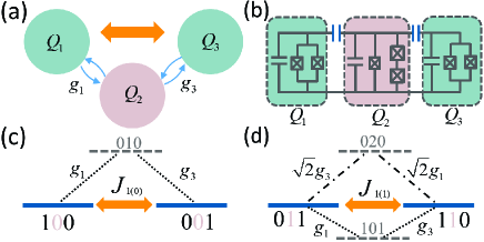
Figure 1: (a) Sketch of an -A-B-A-type three-qubit system with NN coupling. Dispersive interaction between adjacent qubits (denoted as round arrows) can result in an effective NNN coupling (denoted as double-headed arrows). (b) Circuit diagram of a chain of three superconducting qubits capacitively coupled to each other, where the $Q_{1(3)}$ and $Q_{2}$ are transmon qubit R21 and C-shunted flux qubit R22 ; R23 ; R24 , which can be modeled as weak anharmonic oscillators with negative and positive anharmonicity, respectively. (c) For the intermediary qubit $Q_{2}$ in $|0\rangle$ state, the NNN exchange interaction with strength $J_{1(\textbf{0})}$ is enabled by a single path (denoted as dashed lines) involving the intermediate state $|010\rangle$. (d) For $Q_{2}$ in $|1\rangle$ state, the NNN interaction with strength $J_{1(\textbf{1})}$ is enabled by two paths (denoted as dashed lines and dash-dotted lines, respectively), and each involves an intermediate state, i.e., $|101\rangle$ or $|020\rangle$.

In this work, we theoretically explore the possibility of engineering the (intermediary) qubit-mediated NNN coupling in a scalable superconducting quantum processor to implement controlled two-qubit operations where the intermediary qubit controls the operation on the NNN qubits. We demonstrate that, by coupling two types of superconducting qubits with anharmonicities of opposite signs arranged in an -A-B-A- pattern, on the one hand, the unwanted ZZ coupling between adjacent qubits can be heavily suppressed R13 ; R14 , thus breaking the limitation on the performance of potentially implemented native three-qubit gates, on the other hand, a switchable coupling between NNN qubits can be realized R15 , where the intermediary qubit state functions as an on/off switch for this NNN coupling. Thus, depending on the activating scheme, this switchable NNN coupling could be used to realize various controlled two-qubit operations R16 , and a case study shows that controlled-iSWAP (C-iSWAP) gate R17 ; R18 with intrinsic gate fidelity (excluding the decoherence error) in excess of $99.9\,\%$ can be achieved in $50$ ns. We further show that compared with the decomposition methods based on single- and two-qubit gates, textbook three-qubit gates such as Toffoli gate (CCNOT) and Controlled-Controlled-Z gate (CCZ), which are widely used in various quantum circuits R19 , can be constructed efficiently via the native C-iSWAP gate. Moreover, the switchable NNN coupling can also be employed for efficiently generating a continuous set of controlled two-qubit gates for quantum chemistry R20 .

II switchable NNN exchange coupling

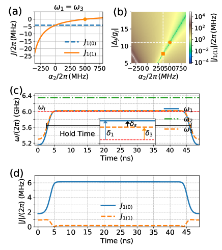
Figure 2: (a) Calculated strength of the effective NNN interactions $J_{1(\textbf{1})}$ and $J_{1(\textbf{0})}$ versus $Q_{2}$’s anharmonicity $\alpha_{2}$ with NN coupling strength $g_{j}/2\pi=45\,\rm MHz$, qubit detuning $\Delta_{j}/2\pi=-500\,\rm MHz$, and qubit anharmonicity $\alpha_{j}/2\pi=-350\,\rm MHz$. The orange dot indicates the working point where the NNN couping is turned off for $Q_{2}$ in $|1\rangle$ state. (b) Calculated values of $J_{1(\textbf{1})}$ versus $\alpha_{2}$ and $\Delta_{j}$ in the unit of $g_{j}$. The anharmonicity $\alpha_{j}$ and NN coupling strength $g_{j}$ take the same values as in (a). The horizontal cut denotes the result plotted in (a), and the intersection (orange square) of the vertical cuts at $\alpha_{2}/2\pi=\,\rm 350MHz$ and the blue strip gives the ideal optimal working point for native C-iSWAP gate operations. (c) Typical control pulse for realizing C-iSWAP gate, where the frequency of $Q_{2}$ is fixed, and the frequencies of $Q_{1}$ and $Q_{3}$ vary from the idle frequency point $\omega_{i}$ to the interaction frequency point $\omega_{I}$ and then come back. The inset highlights the frequency offset $\delta_{1(3)}$ with respect to the ideal interaction point (horizontal red dashed line), where $\delta_{s}=\delta_{1}-\delta_{3}$ denotes a small frequency overshoot. (d) Calculated values of the analytical strength of the effective exchange interactions $J_{1(\textbf{0})}$ and $J_{1(\textbf{1})}$ as a function of time with the typical control pulse (c) applied to the three-qubit system.

To start let us consider an A-B-A type system comprising three superconducting qubits (labeled as $Q_{1,2,3}$, where $Q_{1(3)}$ (A-type qubit) denotes the transmon qubit with negative anharmonicity, and $Q_{2}$ (B-type qubit) represents the capacitively shunted flux qubit with positive anharmonicity R21 ; R22 ; R23 ; R24 ) capacitively coupled to each other, as depicted in Fig. 1, which can be modeled by a chain of three weakly anharmonic oscillators with NN coupling, described by (hereinafter $\hbar=1$)

$$\begin{aligned} H=&\sum_{l}\left[\tilde{\omega}_{l}q_{l}^{\dagger}q_{l}+\frac{\alpha_{l}}{2}q_{l}^{\dagger}q_{l}^{\dagger}q_{l}q_{l}\right]+\sum_{j}g_{j}(q_{j}^{\dagger}q_{2}+q_{j}q_{2}^{\dagger}),\end{aligned}$$ (1)

where the subscript $l={1,2,3}$ labels qubit $Q_{l}$ with anharmonicity $\alpha_{l}$ and bare qubit frequency $\tilde{\omega}_{l}$, $q_{l}\,(q_{l}^{\dagger})$ is the associated annihilation (creation) operator, and $g_{j}$ ($j=1,3$) denotes the strength of the NN coupling between $Q_{j}$ and $Q_{2}$. In the following discussion, we focus on this -A-B-A-type system for implementing switchable NNN coupling and controlled two-qubit gate operations, leaving the extension to the -B-A-B-type system and even the two-dimensional array to the discussion.

We now consider that the system operates in the dispersive regime where the qubit frequency detuning ($\Delta_{j}=\tilde{\omega}_{j}-\tilde{\omega}_{2}$) is far larger than the NN coupling strength, i.e., $|\Delta_{j}|\gg g_{j}$. Thus, by using the Schrieffer-Wolff transformation R25 ; R26 which removes the NN coupling in the Hamiltonian given in Eq. (1), one can obtain an effective block-diagonal Hamiltonian for the full system (see Appendix B for a full derivation). Truncated to the qubit levels, the effective Hamiltonian has the following form (see Appendix B for a full derivation)

$$\begin{aligned} H_{\rm eff}=&\omega_{1}\frac{ZII}{2}+\omega_{2}\frac{IZI}{2}+\omega_{3}\frac{IIZ}{2}+\zeta_{1}\frac{ZZI}{2}+\zeta_{3}\frac{IZZ}{2}\\ &+J_{Z}\frac{XZX+YZY}{2}+J_{I}\frac{XIX+YIY}{2}\\ &+\zeta_{Z}\frac{ZZZ}{2}+\zeta_{I}\frac{ZIZ}{2},\end{aligned}$$ (2)

where $\rm(X,Y,Z,I)$ represent the Pauli operator and identity operators, and the order indexes the qubit number, $\omega_{l}$ and $\zeta_{j}$ denote dressed qubit frequency of $Q_{l}$ and the strength of the ZZ coupling between $Q_{j}$ and $Q_{2}$, respectively. The last four terms represent the effective interaction between NNN qubits ($Q_{1}$ and $Q_{3}$).

In Eq. (2), the terms XZX+YZY and XIX+YIY result in a net virtual exchange interaction between $Q_{1}$ and $Q_{3}$, and the value of its net strength depends on the state of $Q_{2}$. From the view of the second-order perturbation theory, the physics behind this feature is that the virtual exchange interaction results from different contributions, depending on the state of $Q_{2}$. As shown in Fig. 1(c), in an -A-B-A-type three-qubit system where the frequency of $Q_{2}$ satisfies $\tilde{\omega}_{2}>\tilde{\omega}_{j}$, the effective interaction between $|100\rangle$ and $|001\rangle$ with strength $J_{1(\textbf{0})}=J_{I}-J_{Z}=g_{1}g_{3}(\Delta_{1}+\Delta_{3})/(2\Delta_{1}\Delta_{3})$ is enabled by the path given as $|100\rangle\rightarrow|010\rangle\rightarrow|001\rangle$. However, as shown in Fig. 1(d), for the effective interaction $|110\rangle\leftrightarrow|011\rangle$ with strength $J_{1(\textbf{1})}=J_{I}+J_{Z}$ given as

$$\begin{aligned} J_{1(\textbf{1})}=\frac{g_{1}g_{3}}{2}\left[\frac{\Delta_{1}+\alpha_{2}}{\Delta_{1}(\Delta_{1}-\alpha_{2})}+\frac{\Delta_{3}+\alpha_{2}}{\Delta_{3}(\Delta_{3}-\alpha_{2})}\right],\end{aligned}$$ (3)

there are two paths given as $|110\rangle\rightarrow|020\rangle\,(|101\rangle)\rightarrow|011\rangle$, and since $\tilde{\omega}_{2}>\tilde{\omega}_{j}$, the two paths contribute with strength of opposite-sign, enabling competition between the positive and the negative contributions. Thus, one may reasonably expect that by engineering the system parameters, the strength of the dispersive interactions $J_{1(\textbf{1})}$ can take a value of $0$ when the two competitive contributions destructively interferes, while $J_{1(\textbf{0})}$ is intact.

For our proposed -A-B-A-type system shown in Fig. 1(c), the B-type qubit (C-shunt flux qubit) has an positive anharmonicity, i.e., $\alpha_{2}>0$, and the qubit detuning $\Delta_{j}<0$. When $\alpha_{2}=-\Delta_{1}=-\Delta_{3}$, the two competitive contributions in Eq. (3) yield zero net coupling strength $J_{1(\textbf{1})}=0$. Thus, a switchable NNN coupling can be realized. In addition, according to Eq. (3), a similar result can also be obtained for a -B-A-B-type three-qubit system, where the anharmonicity of A-type qubit (transmon qubit) takes a negative value $\alpha_{2}<0$, and the frequency of $Q_{2}$ satisfies $\tilde{\omega}_{2}<\tilde{\omega}_{j}$, thus a switchable NNN coupling can also be realized with $\alpha_{2}=-\Delta_{1}=-\Delta_{3}$ (see Appendix C for details).

According to Eq. (3), Figure $2$(a) shows the calculated $J_{1(\textbf{1})}$ and $J_{1(\textbf{0})}$ versus the $Q_{2}$ anharmonicity $\alpha_{2}$ for system parameters given as: $g_{j}/2\pi=45\,\rm MHz$, $\Delta_{j}/2\pi=-500\,\rm MHz$, and $\alpha_{j}/2\pi=-350\,\rm MHz$. One can find that when $\alpha_{2}/2\pi$ takes a value of $500\,\rm MHz$, i.e., $\alpha_{2}=-\Delta_{1(3)}$, the NNN coupling strength $J_{1(\textbf{1})}$ is zero for $Q_{2}$ in $|1\rangle$, while for $Q_{2}$ in $|0\rangle$, since the coupling strength $J_{1(\textbf{0})}$ is independent of $\alpha_{2}$, the interaction is intact, thus allowing us to control the NNN coupling with a high on/off ratio, where the state of $Q_{2}$ functions as an on/off switch. Therefore, at the working point $\alpha_{2}=-\Delta_{1(3)}$, the effective NNN coupling can be described by

$$\begin{aligned} H_{\rm CXY}=J_{1(\textbf{0})}[|0\rangle\langle 0|]_{2}\otimes\big{(}[|01\rangle\langle 10|]_{1,3}+[|10\rangle\langle 01|]_{1,3}\big{)}.\end{aligned}$$ (4)

Similar result can also be obtained for the terms ZZZ and ZIZ in Eq. (2), which describe the dispersive ZZ coupling between $Q_{1}$ and $Q_{3}$ resulting from the virtual exchange interaction between qubit states and non-qubit states, the interaction strength of which also depends on the state of $Q_{2}$, thus enabling the ZZ interaction controlled by the state of $Q_{2}$ (see Appendix D for details).

III Realization of Controlled-$\rm i$SWAP gate

Table 1: System parameters used for implementing the C-iSWAP gate.

Qubits	$Q_{1}$	$Q_{2}$	$Q_{3}$
Anharmonicity $\alpha/2\pi\,(\rm MHz)$	-350	350	-350
Idle frequency $\omega_{i}/2\pi\,(\rm GHz)$	5.15	6.35	5.30
Interaction frequency $\omega_{I}/2\pi\,(\rm GHz)$	$\sim$6.00	6.35	$\sim$6.00
NN coupling strength $g/2\pi\,(\rm MHz)$	45       45

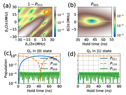
Figure 3: Optimal working point for C-iSWAP gate. (a) Swap error $1-P_{011}$ versus the frequency offset $\delta_{1}$ and $\delta_{3}$ that are defined with respect to the ideal interaction point, as shown in the inset of Fig. 2(c). The system is initialized in the eigenstate $|\widetilde{011}\rangle$ at the idle point, and the hold time takes a value of 45 $\rm ns$. The (orange) square indicates the working point where the NNN exchange interaction is turned off for $Q_{2}$ in $|1\rangle$. (b) Population $P_{001}$ versus the overshoot $\delta_{s}=\delta_{1}-\delta_{3}$ and hold time for system initialized in the eigenstate $|\widetilde{001}\rangle$ at the idle point. The horizontal cut (dashed line) depicts the optimal value of overshot for enabling a full complete swap betweeen $|\widetilde{001}\rangle$ and $|\widetilde{100}\rangle$. (c) Population swap $|\widetilde{001}\rangle\Leftrightarrow|\widetilde{100}\rangle$ and (d) $|\widetilde{011}\rangle\Leftrightarrow|\widetilde{110}\rangle$ versus hold time for system initialized in $|\widetilde{100}\rangle$ and $|\widetilde{110}\rangle$, respectively. With optimal frequency offset and overshot obtained from (a) and (b), the NNN exchange interaction is turned on or off depending on the state of $Q_{2}$.

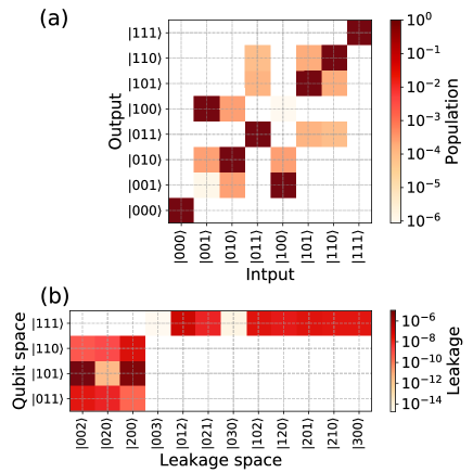
Figure 4: C-iSWAP gate implementation. (a) C-iSWAP gate truth table from the numerical simulation with the system initialized in the logical basis state. For each input state taken from logical basis, the output state shows an agreement with the expected result from the ideal C-iSWAP. (b) Leakage during the gate implementation from the numerical simulation with the system initialized in the qubit subspace that is susceptible to leakage error. Leakage to non-qubit state is suppressed below $10^{-5}$.

Having shown the switchable two-qubit exchange coupling, we now turn to use it to demonstrate controlled two-qubit operations. From Eq. (4), it becomes clear that the switchable NNN coupling at the working point could be used to realize the C-iSWAP gate with an arbitrary swap angle $\theta$, i.e.,

$$U_{CXY}(\theta)=\left(\begin{array}[]{cccccccc}1&0&0&0&0&0&0&0\\ 0&\cos{\frac{\theta}{2}}&0&0&i\sin{\frac{\theta}{2}}&0&0&0\\ 0&0&1&0&0&0&0&0\\ 0&0&0&1&0&0&0&0\\ 0&i\sin{\frac{\theta}{2}}&0&0&\cos{\frac{\theta}{2}}&0&0&0\\ 0&0&0&0&0&1&0&0\\ 0&0&0&0&0&0&1&0\\ 0&0&0&0&0&0&0&1\\ \end{array}\right)$$ (5)

which becomes a C-iSWAP gate for $\theta=\pi$. However, we note that since this effective coupling results from dispersive NN coupling (second-order process), its coupling strength has a magnitude similar to the residual dispersive coupling between adjacent qubits that are presented in the full system effective Hamiltonian $H_{\rm eff}$, i.e., ZZ coupling terms $\rm ZZI$ and $\rm IZZ$ R11 (while terms $\rm ZIZ$ and $\rm ZZZ$ are originated from fourth-order process R12 , see also in Appendixes B and D). Hence, these residual interactions impose a limiting factor on the fidelity of the native C-iSWAP gate.

As demonstrated in the previous study R14 , in order to suppress the unwanted ZZ coupling between adjacent qubits in the present system where qubits are coupled together directly via a capacitor, the anharmonicity of $Q_{2}$ should have a similar magnitude to those of the two adjacent qubits $Q_{1}$ and $Q_{3}$. This means that the optimal working point for realizing C-iSWAP gate using the NNN coupling is $\alpha_{2}=-\Delta_{1(3)}=-\alpha_{1(3)}$, as shown in Fig. 2(b), where the calculated $J_{1(\textbf{1})}$ versus the anharmonicity $\alpha_{2}$ and the qubit frequency detuning $\Delta_{j}$ with system parameters $g_{j}/2\pi=45\,\rm MHz$ and $\alpha_{j}/2\pi=-350\,\rm MHz$ is presented according to Eq. (3).

Based on the above analysis, in the following discussion, we show a case study that explores the switchable NNN coupling in a three-qubit system with always-on interaction to implement the C-iSWAP gate. The system parameters are tabulated in Table $\rm I$. During the implementation of the three-qubit gate, the frequency of the intermediary qubit $Q_{2}$ is fixed, and the frequencies of the two NN qubits $Q_{1}$ and $Q_{3}$ vary from the idle frequency point $\omega_{i}$ to the interaction frequency point $\omega_{I}$ according to a time-dependent function as shown in Fig. 2(c), where the hold time is defined as the time-interval between the midpoints of the ramps R27 (see Appendix E). According to the analytical derivation of the effective NNN coupling, Figure  2(d) shows the analytical strength of the exchange interactions $J_{1(\textbf{1})}$ and $J_{1(\textbf{0})}$ as a function of time during the typical gate implementation with respect to the control pulse shown in Fig. 2(c). We note that this analytical expression of the exchange interactions is derived based on the basis that is dressed by the NN coupling between $Q_{2}$ and $Q_{j}$ (the full system Hamiltonian $H$ is written with a block-diagonal form as $H_{\rm eff}$ in terms of this dressed basis), rather than the logical basis that is defined as the eigenstate of the full system Hamiltonian $H$ at the parking (idling) point (see Appendix A).

Before going further, it is important to note that the above analysis, as well as the optimal working point, is derived based on the analytical expression for $J_{1(\textbf{1})}$ given in Eq. (3), which is valid under the dispersive condition, i.e., $|\Delta_{j}/g_{j}|\gg 1$. However, for a system with parameters tabulated in Table $\rm I$, one may argue that the system operates in a quasi-dispersive regime at the interaction point, where $|\Delta_{j}/g_{j}|=|\alpha_{2}/g_{j}|\approx 7.78$. Nonetheless, as shown in the following numerical analysis, although operating in the quasi-dispersive regime, the above results do approximate the full system dynamics well.

In order to find the optimal working point numerically, firstly, according to the expression given in Eq. (3), we estimate the time $T$ for realizing a full swap when the system is initialized in state $|001\rangle$, giving $T\approx\pi/2J_{1(\textbf{0})}=45\,\rm ns$. Therefore, as shown in Fig. 3(a), by initializing the system in eigenstate state $|\widetilde{011}\rangle$ at the idling point (Note that at the idling point, the inter-qubit coupling is effectively turned off, and the logical basis state is defined as the eigenstates of the system biased at this point, i.e, $|\widetilde{ijk}\rangle$, which is adiabatically connected to the bare state $|ijk\rangle$), and varying the qubit frequencies according to the pulse shown in Fig. 2(c) with hold time of 45 $\rm ns$, we numerically study the swap error defined as $1-P_{011}$ ($P_{011}$ denotes the population in $|\widetilde{011}\rangle$ after the time evolution) versus $\delta_{1}$ and $\delta_{3}$ that are defined as the frequency offsets with respect to the ideal interaction point, as shown in the inset of Fig. 2(c). In Fig. 3(a), the square indicates the working point where the two offsets are equal, i.e., $\delta_{1}=\delta_{3}$, thus preserving on-resonance condition for iSWAP gate, and meanwhile, the swap error is much smaller than other points on the diagonal of the parameter space, which means that at this point, the NNN coupling is turned off for $Q_{2}$ in $|1\rangle$ state. To enable a complete swap in our fixed coupled system that is initialized in state $|\widetilde{001}\rangle$, we further consider a small frequency overshoot $\delta_{s}=\delta_{1}-\delta_{3}$ applied on $Q_{1}$ R28 , as shown in the inset of Fig. 2(c), and the horizontal dashed line in Fig. 3(b) depicts the optimal value of the overshot for this purpose.

Hence, with the optimal frequency offset and overshoot obtained from the above numerical analysis, Figures  3(c) and 3(d) show the state population versus hold time for system initialized in eigenstate state $|\widetilde{100}\rangle$ and $|\widetilde{110}\rangle$ at the idle point, respectively. One can find that for $Q_{2}$ prepared in $|0\rangle$, the NNN exchange interaction is turned on, enabling an almost complete population swap between $Q_{1}$ and $Q_{3}$ ($|\widetilde{001}\rangle\Leftrightarrow|\widetilde{100}\rangle$), while for $Q_{2}$ prepared in $|1\rangle$, the exchange interaction is turned off, thus there is no population swap between $Q_{1}$ and $Q_{3}$. Moreover, although operating in the quasi-dispersive regime, during the time evolution, the population in $Q_{1}$ or $Q_{3}$ leaking to $Q_{2}$ can still be strongly suppressed, as shown in Figs. 3(c) and 3(d).

As already mentioned before, a direct application of the switchable NNN coupling demonstrated in Fig. 3 is the implementation of the $U_{\rm CXY}(\theta)$ gate given in Eq. (5). Here, for illustration purpose, we consider the implementation of C-iSWAP gate, i.e., $U_{\rm CXY}(\pi)$, which is realized with a hold time of $43.2\,\rm ns$, as shown in Fig. 3. By preparing system in eight logical basis states (eigenstates at the idle point), Figure 4 (a) shows the output basis state, exhibiting good agreement with the expected result from the ideal C-iSWAP.

III.1 Intrinsic gate performance

To quantify the intrinsic gate performance of the implemented C-iSWAP gate, we consider the average gate fidelity defined as R29

$$\begin{aligned} F=\frac{{\rm Tr}(UU^{{\dagger}})+|{\rm Tr}(U_{CXY}(\pi/2)U^{{\dagger}})|^{2}}{72},\end{aligned}$$ (6)

where $U$ is the actual evolution operator (excluding the effect of the decoherence process) in terms of the logical basis. This is calculated with the full system Hamiltonian of Eq. (1), where each qubit are modeled as a four-level system (see Appendix E for more details). Truncated to the qubit levels, and up to single-qubit phase gates and a global phase R27 ; R30 ; R31 (see also Appendix E for details), we find that our gate has an intrinsic fidelity of $F=99.97\%$ for gate time in $50$ $\rm ns$. Aside from the control error, this high intrinsic gate fidelity is enabled by (i) the low leakage error, as shown in Fig. 4(b), where one can find that the leakage to non-qubit state is suppressed below $10^{-5}$, (ii) lower coherence phase error, which is caused by parasitic ZZ coupling between qubits, as tabulated in Table $\rm II$, the accumulated phase resulting from the interaction between qubit state and non-qubit is suppressed below $0.02\,\rm rad$.

Furthermore, from Table $\rm II$, one can find that the coherence phases accumulated in state $|\widetilde{011}\rangle$ and $|\widetilde{110}\rangle$ are smaller than $0.005\,\rm rad$. Considering the rather strong NN coupling, these rather low accumulated phases demonstrate that by coupling two-type of qubits with opposite-sign anharmonicities together, the residual ZZ interaction is heavily suppressed, as shown in previous studies R13 ; R14 . And since the coupling between NNN qubits is enabled by second-order process, and the qubits have a considerably larger anharmonicity, the ZZ coupling between NNN qubits is also suppressed (note that as mentioned above, the virtual exchange interactions between qubit state and non-qubit state are dependent on the state of $Q_{2}$ (see Appendix E), thus the accumulated phases in $|\widetilde{101}\rangle$ and $|\widetilde{111}\rangle$ are different). However, we note that aside from the leakage error, as in the case of two-qubit iSWAP gate R28 ; R32 ; R33 , this residual ZZ coupling between NNN qubits imposes a fundamental tradeoff between the fidelity of C-iSWAP gate and the gate speed.

Although the above demonstration has shown that the native implementation of C-iSWAP gate with high intrinsic fidelity and shorter gate time should be possible with realistic parameters, we note that these successes are based on a rather strong NN coupling (although feasible with present technology, but it is larger than the typical NN coupling commonly used in practice R4 ; R34 ) and the qubit frequency with a larger tunable range. In practice, the strong always-on coupling in the present work may make single qubit addressing R35 , as well as the implementation of the two-qubit gates R4 ; R34 , a challenge for system with limited frequency tunability. However, we find that with a smaller NN coupling with strength of $30\,\rm MHz$ R4 , the intrinsic gate fidelity above $99\%$ ($99.9\%$) can still be achieved in 50 (100) $\rm ns$ (see Appendix E). Moreover, the present protocol could also be applied to the system with tunable NN coupling R5 ; R36 ; R37 ; R38 , thus removing the above mentioned constrains.

Table 2: Accumulated coherence phase caused by the parasitic ZZ coupling between qubits during the gate implementation.

	011	101	110	111
Phase ($\phi\times 10^{-3}\,\rm rad$)	-4.40	-17.28	-3.67	8.67

III.2 Impact of decoherence process

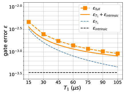
Figure 5: Relation between gate infidelity $\varepsilon$ and qubit relaxation time $T_{1}$ (here assuming that qubit dephasing time $T_{\phi}=\infty$). Since $T_{1}$ of the C-shun flux qubit can have a magnitude comparable to that of the Transmon qubit, here $T_{1}$ of the three qubits takes the same value. $\varepsilon_{\rm full}=1-F_{o}$ denotes the gate infidelity, that is obtained by solving the Lindblad master equation in the Liouville representation, $\varepsilon=1-F$ represents the intrinsic gate infidelity, and $\varepsilon_{T_{1}}$ corresponds to the infidelity assuming only $T_{1}$ decay.

Here we evaluate the impact of relaxation effect on our proposed gate implementation. Since the fidelity $F$ defined in Eq. (6) is no longer valid in the presence of decoherence process, we will instead use the average gate fidelity $F_{o}$ defined as R29 ; R39 ; R40 ; R41

$$\begin{aligned} F_{o}=\frac{8(1-L_{1})+{\rm Tr}(\mathcal{P}_{U}^{{\dagger}}\mathcal{P}_{U_{\rm{target}}})}{72},\end{aligned}$$ (7)

where $\mathcal{P}_{U}$ denotes the system time-evolution superoperator, that is obtained by solving the Lindblad master equation in the Liouville representation R42 ; R43 (see Appendix E for more details), $\mathcal{P}_{U_{\rm{target}}}=U_{\rm{target}}^{\ast}\otimes U_{\rm{target}}$ (Here $U_{\rm target}=U_{\rm CXY}(\pi/2)$) denotes the target gate operation in the Liouville representation, and $L_{1}$ denotes the leakage of the gate operation, given as R39 ; R40

$$\begin{aligned} L_{1}=1-\frac{1}{8}\sum_{i,j,k\in\{0,1\}}{\rm Tr}(\mathcal{P}_{U}|ijk\rangle\rangle),\end{aligned}$$ (8)

where $|ijk\rangle\rangle$ denotes the logical qubit state $|ijk\rangle$ represented in the Liouville space. We note that by ignoring the decoherence process, the above defined average gate fidelity $F_{o}$ is consistent with the fidelity $F$ of Eq. (6) R29 ; R39 ; R40 ; R41 .

According to the above defined fidelity $F_{o}$, Figure 5 shows the relation between gate infidelity $\varepsilon_{\rm full}=1-F_{o}$ and qubit relaxation time $T_{1}$ (here assuming that qubit dephasing time $T_{\phi}=\infty$). We note that at current state, the typical value of $T_{1}$ of the C-shun flux qubit can have a magnitude comparable to that of the Transmon qubit R24 , thus $T_{1}$ of the three qubits takes the same value in our numerical analysis. In Fig. 5, we have also shown the intrinsic gate infidelity $\varepsilon=1-F$ and the infidelity assuming only $T_{1}$ decay (see Appendix E for more details) R29

$$\begin{aligned} \varepsilon_{T_{1}}\approx 3\left[1-\frac{3+e^{-t/T_{1}}+2e^{-t/2T_{1}}}{6}\right].\end{aligned}$$ (9)

From Fig. 5, one can find that gate fidelity of $99.5\%$ ($99.9\%$) could be achieved with qubit relaxation time $T_{1}\geq 15\,\mu s$ ($T_{1}\geq 105\,\mu s$). In Fig. 5, we also show that combining the intrinsic gate infidelity and the infidelity assuming only $T_{1}$ decay gives an estimated value of the gate infidelity $\varepsilon+\varepsilon_{T_{1}}$, which is in good agreement with $\varepsilon_{\rm full}$.

In the discussion above, we have omitted the effect of the qubit dephasing process ($T_{\phi}=\infty$). Here, we give an estimate of the effect of the qubit dephasing process (white noise) on the gate performance. With current superconducting qubits, the qubit dephasing time (white noise) can commonly reach up to $T_{\phi}=2T_{1}$ R44 , giving the infidelity assuming only $T_{1}$ and $T_{\phi}$ process as

$$\varepsilon_{T_{1}} \approx 3\left[1-\frac{3+e^{-t/T_{1}}+2e^{-t(1/2T_{1}+1/T_{\phi})}}{6}\right]$$ (10)

$$\approx\frac{t}{T_{1}}+\frac{t}{T_{\phi}}.$$

Thus, one may reasonably estimate that C-iSWAP gate with fidelity in excess of $99\%$ could be attainable with current technology, and gate infidelity primarily results from qubit relaxation.

IV Possible application of the $U_{\rm CXY}$ gates

Here we discuss two possible applications of our proposed native three-qubit gates $U_{\rm CXY}(\theta)$, and show that compared with a quantum processor having only native single- and two-qubit gates, implementing native three-qubit gates can potentially reduce circuit depth or gate count of quantum circuits, such as a three-qubit Toffoli gate and controlled-XX (controlled-YY/ZZ) evolution with arbitrary rotation angle $\theta$ for quantum chemistry using the quantum phase estimation algorithm (PEA) R20 . We note that our proposed controlled two-qubit operation is based on the effective switchable NNN exchange coupling, which is turned on (off) when the intermediary qubit is at its ground state (excited state). Thus, following the convention taken in quantum computing community, one may relabeled the ground state (excited state) of the intermediary qubit as its logical state $|1\rangle$ ($|0\rangle$).

IV.1 The three-qubit Toffoli gate

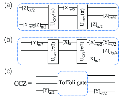
Figure 6: Quantum circuit diagram decomposition of the three-qubit Toffoli gate and CCZ gate with $U_{\rm CXY}(\theta)$ and single qubit gates $[\mathcal{O}]_{\theta}\equiv\rm{exp}[-i\theta(\mathcal{O}/2)]$. (a) Implementation of the Toffoli gate with $U_{\rm CXY}(\pi)$ (C-iSWAP gate). (b) Implementation of the Toffoli gate with $U_{\rm CXY}(\pi/2)$ (C-$\sqrt{\rm{iSWAP}}$ gate). (c) Implementation of CCZ gate with quantum circuit in (a) or (b).

The textbook three-qubit gate Toffoli gate, which is widely used in various quantum circuits R19 , in general cannot be implemented natively R45 ; R46 ; R47 without resorting to the decomposition approach that involves a series of gate sequences including single- or two-qubit gates. Even with the decomposition approach, the circuit depths and gate count needed for implementing Toffoli gate depend heavily on the available native gate set R45 ; R46 ; R47 ; R48 . For a fully connected quantum processor with native gate set including one- and two-qubit gates, the most common approach for realizing Toffoli gate requires six CNOT gates or CZ gates and multiple one-qubit gates R45 , while in a quantum processor with NN coupling, which is one of the most native architectures for realizing a scalable superconducting quantum processor, since the available native two-qubit gate is only possible for pair of NN qubits, more two-qubit gates are needed on account of this limited connectivity R45 ; R48 . However, as shown in Figs. 6(a) and 6(b), a Toffoli gate can be implemented via our proposed native controlled two-qubit peration with only two applications of $U_{\rm CXY}(\pi)$ (a simple extension of the results in Ref. R45 ) or $U_{\rm CXY}(\pi/2)$ (a simple extension of the results in Ref. R49 ), thus heavily reducing the circuit depth and gate count. As shown Figs. 6(c), with two additional one-qubit gates, the CCZ gate can also be constructed by using only two $U_{\rm CXY}(\pi)$ or $U_{\rm CXY}(\pi/2)$. Therefore, one may reasonably estimate that using the above decomposition method with native three-qubit gates $U_{\rm CXY}(\theta)$ could improve the performance of the implemented quantum circuits and increase in success probability, especially, in the NISQ era.

IV.2 Controlled-XX rotation in PEA for quantum chemistry

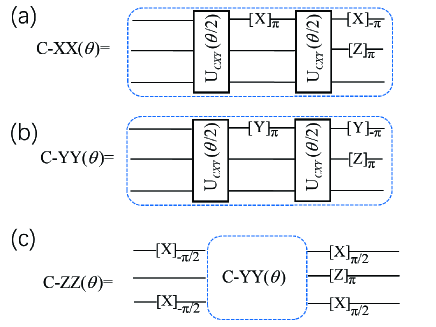
Figure 7: Quantum circuit diagram decomposition of the controlled-XX (YY, ZZ) rotation with an arbitrary angle $\theta$ in terms of $U_{\rm CXY}(\theta/2)$ gates and single-qubit gates $[\mathcal{O}]_{\theta}\equiv\rm{exp}[-i\theta(\mathcal{O}/2)]$. (a),(b) Construction of CXX($\theta$) and CYY($\theta$) with $U_{\rm CXY}(\theta/2)$. (c) Construction of CZZ($\theta$) with quantum circuit in (b).

Figures 7(a) and 7(b) show that based on our proposed three-qubit operation $U_{\rm CXY}(\theta)$, controlled-XX (controlled-YY) operations with arbitrary rotation angle $\theta$, i.e., ${\rm CXX}(\theta)$, ${\rm CYY}(\theta)$, can be constructed via the application of two $U_{\rm CXY}(\theta/2)$. Moreover, with five additional one-qubit gates, controlled-ZZ operation can also be implemented as shown in Fig. 7(c). Having access to these continuous sets of controlled two-qubit rotations may provide more efficient compiled circuits for quantum application such as quantum simulation of Fermionic Hamiltonian R17 ; R50 and quantum chemistry R20 . As a simple example we consider the application of these continuous sets of controlled two-qubit rotations in PEA for quantum chemistry, where the controlled two-qubit rotations are needed for implementing trotterized time-evolution operator R20 . By using the standard decomposition procedure with only one- and two-qubit gates, a ${\rm CXX}(\theta)$ or ${\rm CYY}(\theta)$ operation requires two CNOT gates and one C-Phase gate with phase angle $\theta$ and six single qubits to be implemented on quantum processor with NN coupling, yielding a quantum circuit with gate depth of 5 and gate count of 8 R20 . Moreover, for a quantum processor with only one type of native two-qubit gate, e.g., CZ gate, more additional single qubit gates are needed (implementing a CNOT gate requires one CZ gate and two single qubit gates), thus increasing the circuit depth to 7. As shown in Fig. 7(a), the ${\rm CXX}(\theta)$ can be implemented with gate depth of 4 and gate count of 4. Thus, the continuous sets of controlled two-qubit rotations $U_{\rm CXY}(\theta)$ presented in this work could be useful for quantum simulation and may provide a more efficient compilation for certain quantum circuits.

V Discussion

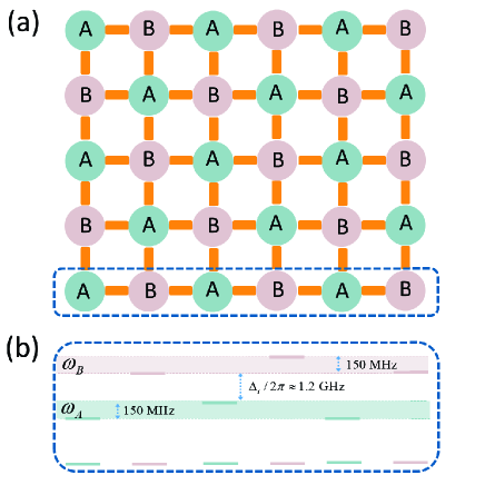
Figure 8: (a) A scalable two-dimentional qubit lattice, where circles at the vertices denote qubits, and yellow lines indicate couplers between adjacent qubits. The lattice comprises two types of qubits (labeled as A and B) that are arranged in an -A-B-A-B- pattern in each row and column. (b) Frequency arrangement in each row and column follows a zigzag pattern with A-type qubit at lower frequency band ($\omega_{A}$) and B-type qubit at higher frequency band ($\omega_{B}$).

As we have discussed in Sec. II (see also in Appendix C), the proposed scheme for realizing switchable NNN coupling can be applied to the -A-B-A- and -B-A-B-type system, where the A-type (B-type) has a negative (positive) anharmonicity, and the qubit frequency of B-type qubit is larger than that of the A-type qubit. We also show that one of the most promising implementation of our proposed superconducting qubit architecture is a superconducting quantum processor comprising transmon qubit (A-type) and C-shunt flux qubit (B-type) arranged in an -A-B-A-B- pattern. Therefore, the proposed scheme can also be applied to a two-dimensional (2D) qubit lattice with NN coupling. An example for 2D qubit lattice with fixed NN coupling is shown in Fig. 8, where the two-type qubits are arranged in an -A-B-A-B- pattern in each row and column, and the arrangement of qubit frequency in each row and column follows a zigzag pattern, i.e, A-type qubit at lower frequency band with typical value of $\omega_{A}$ and B-type qubit at higher frequency band with typical value of $\omega_{B}$ ($\omega_{B}>\omega_{A}$). As demonstrated in Sec. II, at the interaction point (turning on the effective NNN coupling), frequency detuning $\Delta_{i}=\omega_{B}-\omega_{A}$ approaches the magnitude of the qubit anharmonicity $|\alpha|$, and the frequencies of the two target NNN qubit is almost equal to each other. At the parking (idling) point, i.e., turning off the effective NNN coupling, the frequency detuning $\Delta_{i}$ should be far larger that the NN coupling strength (typically, $1.2\,\rm GHz$ vs $45\,\rm MHz$) R4 , as shown in Fig. 8(b). Moreover, in order to further suppress the residual coupling between NNN qubit (typically the strength is about $1.7\,\rm MHz$ here), frequency degeneracy in higher or lower frequency band breaks, yielding a qubit frequency detuning between NNN qubits about $150\,\rm MHz$ .

For practically implementing our scheme in the proposed 2D qubit lattice with fixed NN coupling shown in Fig. 8, where $A$ (B) label transmon qubit (C-shunt flux qubit), special attention should be paid to the following two points, (i) the anharmonicity of the transmon qubit is only weakly dependent on its qubit frequency, thus it is nearly fixed over a tunable range of approximately $1.0\,\rm GHz$ R28 . while for the C-shunt flux qubit, the qubit anharmonicity is strongly dependent on its qubit frequency R13 ; R24 . Moreover, in order to suppress parasitic ZZ interaction between NN qubits, which can lead to conditional phase error during gate operations R14 , the C-shunt flux qubit should has an anharmonicity with magnitude comparable to that of the transmon qubit. This imposes a limitation on the tunable range of the C-shunt flux qubit in our scheme. Thus, to implement our scheme in the 2D qubit lattice, the maximum tunable range of each C-shunt flux qubit could be set below $150\,\rm MHz$, which is adequate for suppressing the parasitic ZZ coupling, and for providing a sufficient tunable range for implementing high on-off ratio NNN coupling in a -B-A-B-type system or the 2D lattice shown in Fig. 8(a). (2) High on-off ratio of the switchable NNN coupling is highly desired for practical purpose. Since the proposed switchable NNN coupling is enabled by dispersive (quasi-dispersive) interaction between NN qubits, a strong NN coupling is required for realizing fast gates, thus reducing the decoherence error. Meanwhile, a larger qubit detuning between NN qubits is needed for turning it off effectively. Overall, the two points imply that a larger tunable range of the transmon qubit is needed for practical implementation of our scheme. However, for transmon qubit far away from its maximum frequency point (flux insensitive point), the coherence time is commonly heavily suppressed (due to the influence of $1/f$ magnetic flux noise), causing gate infidelity. Hence, the speed-fidelity tradeoff needs to be understood carefully for implementing our scheme in the proposed 2D qubit lattice with fixed NN coupling. It is worth noting that although a fixed NN coupling is assumed in the demonstration of the switchable NN coupling in Set. II and in the above discussion on the scalability of our scheme, the proposed scheme is obviously also compatible with the qubit lattice with tunable NN coupling R5 ; R36 ; R38 , thus relaxing above mentioned constraints.

Finally, we note that our proposed scheme for implementing native C-iSWAP gate is based on effective three-qubit interaction resulting from NN transverse (XY) coupling, and the control pulse is described by only a few parameters (e.g., frequency offset $\delta_{j}$, frequency overshoot $\delta$, and hold time, as shown in Fig. 2), making the in situ experimental optimization of pulse parameters as feasible as the case for the typical one- or two-qubit gate operations, for which the in situ optimization of pulse parameters has been shown as a key step towards high-fidelity gate operations R51 ; R52 . For system with NN transverse coupling, an alternative (single-shot) scheme for implementing C-iSWAP gate without resorting to the standard decomposition procedure has also been proposed previously by using quantum optimal control R17 , where control pulses are discretized into pixels, and in principle can generate gates with speed approaching the quantum speed limit. However, the success of the optimal control is based on the assumption that accurate knowledge of the practical system parameters is available for optimizing control pulse in theoretical simulation, and for superconducting qubits, this is often not the case in reality R51 ; R52 ; R53 . Moreover, the in situ optimization of pulse parameters is hindered by the larger number of pixels, which in principle could be overcome by using simple parameterizations for the control pulse, such as Fourier and erf parameterizations R53 . Recently, another scheme for implementing native C-iSWAP gate was proposed for superconducting qubit systems with dedicated designed NN coupling R18 , i.e., combining the NN transverse (XY) coupling and the NN longitude (ZZ) coupling, which seems a highly designed asymmetry architecture, potentially limiting the compatibility with existing scheme for realizing high-fidelity one- or two-qubit operations. Therefore, this scheme may be more suitable for certain types of quantum computing applications R18 .

VI Conclusion

In this work, we employ a scalable chain of nearest-neighbor-coupled superconducting qubit system comprising two-type superconducting qubits with opposite-sign anharmonicity to realize switchable coupling between next-nearest-neighboring (NNN) qubits. This switchable coupling is controlled by the state of the intermediary qubit, thus potentially enabling the implementation of various native controlled two-qubit operations. With realistic parameters, we show that it is possible to realize a C-iSWAP gate with an intrinsic average fidelity of $99.9\,\%$ in 50 $\rm ns$. These native implementations of three-qubit gates may find useful application for reducing circuit depth of NISQ algorithms R6 , such as quantum chemistry R20 , and for performing quantum simulations R49 ; R54 .

Appendix A effective Hamiltonian for qubit system

As described in the main text, we consider a linear chain of three superconducting qubits with nearest-neighbor coupling, and here each qubit is treated as an ideal two-level system, thus described by the Hamiltonian $H=H_{0}+V$ with $H_{0}=\sum_{l=1}^{3}\tilde{\omega}_{l}\sigma_{l}^{z}/2$ and

$$\begin{aligned} V=\sum_{j=1,3}g_{j}(\sigma_{j}^{+}\sigma_{2}^{-}+\sigma_{j}^{-}\sigma_{2}^{+}),\end{aligned}$$ (11)

where $\sigma_{j}^{z,\pm}$ denote the Pauli operators associated with the $j$th qubit labeled as $Q_{j}$ with bare qubit frequency $\tilde{\omega}_{j}$, and $g_{j}$ represents the coupling strength between nearest neighbor qubits $Q_{j}$ and $Q_{2}$.

We now turn to derive an effective Hamiltonian for this three-qubit system, and start from the original Hamiltonian $H$, which is composed of an unperturbed part $H_{0}$ with known eigenvalues and eigenstates and a small perturbation part $V$. We consider that the three-qubit system operates in the dispersive regime, where the detuning between nearest-neighbor qubit pair is larger than the coupling strengths between them, thus $|\Delta_{j}|=|\tilde{\omega}_{j}-\tilde{\omega}_{2}|\gg g_{j}$.

For a system operating in the dispersive coupling regime, we can eliminate the direct qubit-qubit coupling $V$ via a unitary transformation R25

$$\begin{aligned} H_{\textrm{eff}}=\exp(-X)H\exp(X),\end{aligned}$$ (12)

where $X$ is chosen such that the direct coupling between the nearest-neighbor qubit pairs in the transformed Hamiltonian disappears. By choosing

$$\begin{aligned} X=\frac{g_{1}}{\Delta_{1}}(\sigma_{1}^{-}\sigma_{2}^{+}-\sigma_{1}^{+}\sigma_{2}^{-})+\frac{g_{3}}{\Delta_{3}}(\sigma_{3}^{-}\sigma_{2}^{+}-\sigma_{3}^{+}\sigma_{2}^{-}),\end{aligned}$$ (13)

one can prove that it satisfies $[H_{0},X]=-V$. Expanding to the second order of the small parameters ($\frac{g_{j}}{\Delta_{j}}=O(\lambda)$) yields

$$\begin{aligned} H_{\textrm{eff}}&=H_{0}+\frac{1}{2}[V,X]+O(\lambda^{3})\\ &\approx\sum_{l=1}^{3}\frac{\omega_{l}}{2}\sigma_{l}^{z}+J(\sigma_{1}^{+}\sigma_{3}^{-}+\sigma_{1}^{-}\sigma_{3}^{+})\sigma_{2}^{z},\end{aligned}$$ (14)

with

$$\begin{aligned} &\omega_{1}=\tilde{\omega}_{1}+\frac{g_{1}^{2}}{\Delta_{1}},\\ &\omega_{2}=\tilde{\omega}_{2}-(\frac{g_{1}^{2}}{\Delta_{1}}+\frac{g_{3}^{2}}{\Delta_{3}}),\\ &\omega_{3}=\tilde{\omega}_{3}+\frac{g_{3}^{2}}{\Delta_{3}},\\ &J=-\frac{g_{1}g_{3}}{2}(\frac{1}{\Delta_{1}}+\frac{1}{\Delta_{3}}),\end{aligned}$$ (15)

where $\omega_{l}$ are the dressed qubit frequencies of $Q_{l}$, and $J$ is the effective three-qubit interaction strength (next-nearest neighbor coupling) given as $J=-g_{1}g_{3}(\Delta_{1}+\Delta_{3})/(2\Delta_{1}\Delta_{3})$. From Eq. (A4), one can find that the magnitude of the dispersive XY interaction between $Q_{1}$ and $Q_{3}$ is independent of the state of $Q_{2}$, while the sign of the interaction is set by the $Q_{2}$ state, i.e., for $Q_{2}$ in $|0\rangle$ or $|1\rangle$, the value of the interaction strength has an opposite sign. Thus, the effective interaction between $Q_{1}$ and $Q_{3}$ is in fact a three-body interaction.

We note that the original Hamiltonian $H$ is written in the usual bare basis of uncoupled system eigenstates, i.e., eigenstates of the unperturbed Hamiltonian $H_{0}$, but the derived effective Hamiltonian $H_{\rm eff}$ given in Eq.  (A4) is written in the transformed bare basis defined by the unitary transformation. In fact, for fixed coupled system, quantum information processing is commonly performed in the transformed basis R3 ; R27 , i.e., eigenstates of the idle system Hamiltonian $H$, where qubits are all dispersively coupled to each other, i.e., the strength of the direct or indirect coupling between arbitrary pair of qubits is far smaller than the frequency detuning of the coupled qubits. In this way, at the idle point and in the interaction picture, the system states suffer no dynamic evolution. Therefore, throughout this work, we take all these factors into consideration, implicitly.

Appendix B effective Hamiltonian for qubit system with higher energy levels

Since the superconducting qubit is naturally a multi-level system, especially for qubits with weak anharmonicity such as the transmon qubit and the C-shunted flux qubit, the higher energy levels of qubits have non-negligible effect on the effective coupling derived in the above section where superconducting qubits are treated as an ideal two-level system R21 ; R24 . In the following discussion, we will study the effect of the higher energy levels of qubits on the dispersive next-nearest neighbor coupling.

For a system consisting of three superconducting qubits (labeled as $Q_{1,2,3}$) as described in the main text, they can be modeled by a chain of three weakly anharmonic oscillators with nearest neighbor coupling R21 ; R24 . Thus, the Hamiltonian of this system can be described by $H=H_{0}+V$, with

$$\begin{aligned} &H_{0}=\sum_{l=1}^{3}\bigg{[}\tilde{\omega}_{l}q_{l}^{\dagger}q_{l}+\frac{\alpha_{l}}{2}q_{l}^{\dagger}q_{l}(q_{l}^{\dagger}q_{l}-1)\bigg{]}\\ &V=\bigg{[}g_{1}(q_{1}^{\dagger}q_{2}+q_{1}q_{2}^{\dagger})+g_{3}(q_{3}^{\dagger}q_{2}+q_{3}q_{2}^{\dagger})\bigg{]},\end{aligned}$$ (16)

where the subscript $l={1,2,3}$ labels superconducting qubit $Q_{l}$ with anharmonicity $\alpha_{l}$ and bare qubit frequency $\tilde{\omega}_{l}$, $q_{l}\,(q_{l}^{\dagger})$ is the associated annihilation (creation) operator truncated to the lowest four levels (labeled as $\{|0\rangle,|1\rangle,|2\rangle,|3\rangle\}$), and $g_{j}$ ($j=1,3$) denotes the strength of the coupling between adjacent qubits, i.e., $Q_{j}$ and $Q_{2}$. Again, in the following discussion, we consider that the system operates in the dispersive regime where the qubit frequency detuning ($\Delta_{j}=\tilde{\omega}_{j}-\tilde{\omega}_{2}$) is far larger than the NN coupling strength, i.e., $|\Delta_{j}|\gg g_{j}$.

B.1 Schrieffer-Wolff transformation

To derive an effective Hamiltonian for the three-qubit system, we turn to block-diagonalize the original system Hamiltonian $H=H_{0}+\lambda V$, where $\lambda$ is introduced to show the orders in the perturbation expansion, and would be set to $1$ after the calculations, thus the nearest neighbor coupling between qubits is eliminated and the next-nearest neighbor qubits are directly coupled to each other. By projecting the system onto the zero-excitation and one-excitation subspace of $Q_{2}$, we can further derive an effective Hamiltonian for the next-nearest neighbor qubits with the intermediary qubit in its ground state $|0\rangle$ or excited state $|1\rangle$. This is achieved by using the Schrieffer-Wolff transformation R25 ; R26

$$\begin{aligned} &\,\,\,\,\,\,\,H_{\rm eff}=A^{\dagger}HA\\ &A=e^{-iS},\,\,S=\sum_{n=1}^{\infty}S^{(n)}\lambda^{n}\end{aligned}$$ (17)

Following the methods introduced in Ref.R26 , the effective block-diagonal Hamiltonian for the three-qubit system has the following form

$$H_{\rm eff}=\left(\begin{array}[]{ccccc}H_{0}&\textbf{0}&\textbf{0}&\textbf{0}&\ldots\\ \textbf{0}&H_{1}&\textbf{0}&\textbf{0}&\ldots\\ \textbf{0}&\textbf{0}&H_{2}&\textbf{0}&\ldots\\ \textbf{0}&\textbf{0}&\textbf{0}&H_{3}&\ldots\\ \vdots&\vdots&\vdots&\vdots&\ddots\\ \end{array}\right);$$ (18)

where $H_{\rm\textbf{n}}$ ($\rm n=0,1,2,3,...$) denotes the effective Hamiltonian for the three-qubit system projected onto the n-excitation subspace of $Q_{2}$. Consequently, $H_{0}$ corresponds to the effective Hamiltonian projected onto the zero-excitation subspace of $Q_{2}$, i.e., the effective Hamiltonian for the next-nearest neighbor qubits with $Q_{2}$ in state $|0\rangle$. Truncated to the first three energy levels of qubits, i.e. operating with the basis $\{|000\rangle,\,|001\rangle,\,|100\rangle,\,|101\rangle,\,|002\rangle,\,|200\rangle\}$, $H_{\textbf{0}}$ reads

$$H_{\textbf{0}}=\left(\begin{array}[]{cccccc}0&0&0&0&0&0\\ 0&\omega^{\prime}_{3}&J_{1(\textbf{0})}&0&0&0\\ 0&J_{1(\textbf{0})}&\omega^{\prime}_{1}&0&0&0\\ 0&0&0&\omega^{\prime}_{3}+\omega^{\prime}_{1}&J_{2(\textbf{0}),I}&J_{2(\textbf{0}),II}\\ 0&0&0&J_{2(\textbf{0}),I}&2\omega^{\prime\prime}_{3}+\alpha_{3}&0\\ 0&0&0&J_{2(\textbf{0}),II}&0&2\omega^{\prime\prime}_{1}+\alpha_{1}\\ \end{array}\right)$$ (19)

where $\omega^{\prime}_{j}=\tilde{\omega}_{j}+g_{j}^{2}/\Delta_{j}$ ($j=1,3$) denotes the dressed transition frequency of $Q_{j}$, and $\omega^{\prime\prime}_{j}=\tilde{\omega}_{j}+g_{j}^{2}/(\Delta_{j}+\alpha_{j})$ is defined as an effective dressed qubit frequency, to which the coupling involved with higher energy levels of qubits contributes with an additional term $g_{j}^{2}/(\Delta_{j}+\alpha_{j})$.

$$\begin{aligned} J_{1(\textbf{0})}=\frac{g_{1}g_{3}(\Delta_{1}+\Delta_{3})}{2\Delta_{1}\Delta_{3}}\end{aligned}$$ (20)

represents the strength of coupling within one-excitation manifold $\{|001\rangle$, $|100\rangle\}$ of the NNN qubits, and

$$J_{2(\textbf{0}),I}=\frac{\sqrt{2}g_{1}g_{3}(\Delta_{1}+\Delta_{3}+\alpha_{3})}{2\Delta_{1}(\Delta_{3}+\alpha_{3})},J_{2(\textbf{0}),II}\equiv J_{2(\textbf{0}),I}(1\leftrightarrow 3),$$ (21)

corresponds to the strength of coupling within the two-excitation manifold of NNN qubits $\{|101\rangle$, $|200\rangle$, $|002\rangle\}$, i.e, the interaction $|101\rangle\leftrightarrow|200\rangle$ and the interaction $|101\rangle\leftrightarrow|002\rangle$.

$H_{\textbf{1}}$ represents the effective Hamiltonian projected onto the one-excitation subspace of $Q_{2}$, i.e., the effective Hamiltonian for the next-nearest neighbor qubits with $Q_{2}$ in state $|1\rangle$. Then, truncated to the first three energy levels of qubits, i.e., operating with basis $\{|010\rangle,\,|011\rangle,\,|110\rangle,\,|111\rangle,\,|012\rangle,\,|210\rangle\}$, $H_{\textbf{1}}$ is given as

$$H_{\textbf{1}}=\left(\begin{array}[]{cccccc}E_{010}&0&0&0&0&0\\ 0&E_{011}&J_{1(\textbf{1})}&0&0&0\\ 0&J_{1(\textbf{1})}&E_{110}&0&0&0\\ 0&0&0&E_{111}&J_{2(\textbf{1}),I}&J_{2(\textbf{1}),II}\\ 0&0&0&J_{2(\textbf{1}),I}&E_{012}&0\\ 0&0&0&J_{2(\textbf{1}),II}&0&E_{210}\\ \end{array}\right)$$ (22)

with

$$\begin{aligned} &E_{010}=\omega^{\prime}_{2},\\ &E_{011}=\omega^{\prime}_{2}+\omega^{\prime}_{3}+\zeta^{\prime}_{3},\\ &E_{110}=\omega^{\prime}_{2}+\omega^{\prime}_{1}+\zeta^{\prime}_{1},\\ &E_{111}=\omega^{\prime}_{2}+\omega^{\prime}_{3}+\omega^{\prime}_{1}+\zeta^{\prime}_{3}+\zeta^{\prime}_{1},\\ &E_{012}=\omega^{\prime}_{2}+2\omega^{\prime}_{3}+\alpha_{3}+\delta_{3},\\ &E_{210}=\omega^{\prime}_{2}+2\omega^{\prime}_{1}+\alpha_{1}+\delta_{1},\end{aligned}$$ (23)

where $\omega^{\prime}_{2}=\tilde{\omega}_{2}-g_{1}^{2}/\Delta_{1}-g_{3}^{2}/\Delta_{3}$ denotes the dressed transition frequency of $Q_{2}$, $\zeta^{\prime}_{j}=2g_{j}^{2}(\alpha_{j}+\alpha_{2})/[(\Delta_{j}-\alpha_{2})(\Delta_{j}+\alpha_{j})]$ represents the parasitic $ZZ$ interaction between adjacent qubits $Q_{j}$ ($j=1,3$) and $Q_{2}$, which results from the interaction among higher energy levels of qubits, and

$$\begin{aligned} &\delta_{j}=\frac{g_{j}^{2}(5\alpha_{j}+\Delta_{j}+3\alpha_{2})}{(2\alpha_{j}+\Delta_{j})(\Delta_{j}+\alpha_{j}-\alpha_{2})}-\frac{g_{j}^{2}}{\Delta_{j}},\end{aligned}$$ (24)

represents frequency shift resulting from the interaction among higher energy levels of qubits. $J_{1(\textbf{1})}$ describes the strength of coupling within the one-excitation manifold of next-nearest-neighbor qubits $\{|110\rangle$, $|011\rangle\}$, and is given as

$$\begin{aligned} J_{1(\textbf{1})}=\frac{g_{1}g_{3}}{2}\left[\frac{\Delta_{1}+\alpha_{2}}{\Delta_{1}(\Delta_{1}-\alpha_{2})}+\frac{\Delta_{3}+\alpha_{2}}{\Delta_{3}(\Delta_{3}-\alpha_{2})}\right],\end{aligned}$$ (25)

while $J_{2(\textbf{1}),I(II)}$ corresponds to the strength of coupling within the two-excitation manifold of next-nearest-neighbor qubits $\{|111\rangle$, $|012\rangle$, $|210\rangle\}$, i.e, the interaction $|111\rangle\leftrightarrow|012\rangle$ and the interaction $|111\rangle\leftrightarrow|210\rangle$, and it is given as

$$J_{2(\textbf{1}),I}=\frac{\sqrt{2}g_{1}g_{3}\left(2\Delta_{1}(\Delta_{1}^{2}-\alpha_{2}^{2})+(3\Delta_{1}^{2}-\alpha_{2}^{2})(\alpha_{3}-\Delta_{1}+\Delta_{3})+(\alpha_{2}+\Delta_{1})(\alpha_{3}-\Delta_{1}+\Delta_{3})^{2}\right)}{2\Delta_{1}(\Delta_{1}-\alpha_{2})(\Delta_{3}+\alpha_{3})(\Delta_{3}-\alpha_{2}+\alpha_{3})},J_{2(\textbf{1}),II}\equiv J_{2(\textbf{1}),I}(1\leftrightarrow 3).$$ (26)

From the above result, we can find that: (i) when the anharmonicity of $Q_{2}$ takes a value of $\alpha_{2}=0$, i.e., $Q_{2}$ is a linear resonator, and the expression of $J_{1(\textbf{1})}$ and $J_{2(\textbf{1}),I(II)}$ given above will be reduced to $J_{1(\textbf{0})}$ and $J_{2(\textbf{0}),I(II)}$, respectively, agreeing with the well-known fact that the liner-bus mediated coupling between two qubits is a two-body interaction between qubits. (ii) while for $\alpha_{2}\rightarrow\infty$, $Q_{2}$ can be safely treated as an ideal two-level system, thus $J_{1(\textbf{1})}=-J_{1(\textbf{0})}$ is obtained, as the result shown in Appendix  A.

B.2 Effective three-qubit Hamiltonian

For $Q_{2}$ in its ground state $|0\rangle$, the effective interaction among two-excitation manifold of the pair of nearest-neighboring qubits $Q_{1}$ and $Q_{3}$, i.e., interaction between $|101\rangle$ and $|002\rangle\,(|200\rangle)$ as shown in Fig. 9(a), the strength of which is given in Eq. (B6), causes the $ZZ$ interaction between $Q_{1}$ and $Q_{3}$ with strength given as

$$\begin{aligned} \zeta_{101}=\frac{J_{2(\textbf{0}),I}^{2}}{\Delta-\alpha_{3}}-\frac{J_{2(\textbf{0}),II}^{2}}{\Delta+\alpha_{1}},\end{aligned}$$ (27)

where $\Delta=\omega_{1}-\omega_{3}$. While for $Q_{2}$ in its excited state $|1\rangle$, the strength of the ZZ coupling (resulting from the interaction between $|012\rangle\,(|210\rangle$) and $|111\rangle$, as shown in Fig. 9(b)) is

$$\zeta_{111}=\frac{J_{2(\textbf{1}),I}^{2}}{\Delta-\alpha_{3}+\zeta^{\prime}_{1}+\zeta^{\prime}_{3}-\delta_{3}}-\frac{J_{2(\textbf{1}),II}^{2}}{\Delta+\alpha_{1}-\zeta^{\prime}_{1}-\zeta^{\prime}_{3}+\delta_{1}}.$$ (28)

Truncated to the qubit levels, the effective Hamiltonian of the full system has the following approximate form

$$\begin{aligned} H_{\rm eff}=&\omega_{1}\frac{ZII}{2}+\omega_{2}\frac{IZI}{2}+\omega_{3}\frac{IIZ}{2}+\zeta_{1}\frac{ZZI}{2}+\zeta_{3}\frac{IZZ}{2}\\ &+\frac{J_{1(\textbf{1})}-J_{1(\textbf{0})}}{2}\frac{XZX+YZY}{2}\\ &+\frac{J_{1(\textbf{1})}+J_{1(\textbf{0})}}{2}\frac{XIX+YIY}{2}\\ &+\frac{\zeta_{111}-\zeta_{101}}{4}\frac{ZZZ}{2}+\frac{\zeta_{111}+\zeta_{101}}{4}\frac{ZIZ}{2},\end{aligned}$$ (29)

where $\rm(X,Y,Z,I)$ represent the Pauli operator and identity operators, and the order indexes the qubit number, $\omega_{l}$ denotes dressed qubit frequency given as

$$\begin{aligned} &\omega_{1}=\omega^{\prime}_{1}+\frac{\zeta^{\prime}_{1}}{2}+\frac{\zeta_{111}+\zeta_{101}}{4},\\ &\omega_{2}=\omega^{\prime}_{2}+\frac{\zeta^{\prime}_{1}+\zeta^{\prime}_{3}}{2}+\frac{\zeta_{111}-\zeta_{101}}{4},\\ &\omega_{3}=\omega^{\prime}_{3}+\frac{\zeta^{\prime}_{3}}{2}+\frac{\zeta_{111}+\zeta_{101}}{4},\end{aligned}$$ (30)

$\zeta_{j}$ represents the strength of ZZ coupling between adjacent qubits, i.e., $Q_{1(3)}$ and $Q_{2}$, which is given as

$$\begin{aligned} &\zeta_{1}=\frac{\zeta^{\prime}_{1}}{2}+\frac{\zeta_{111}-\zeta_{101}}{4},\zeta_{3}=\frac{\zeta^{\prime}_{3}}{2}+\frac{\zeta_{111}-\zeta_{101}}{4}.\end{aligned}$$ (31)

Taking

$$\begin{aligned} &J_{Z}=\frac{J_{1}^{(\textbf{1})}-J_{1}^{(\textbf{0})}}{2},J_{I}=\frac{J_{1}^{(\textbf{1})}+J_{1}^{(\textbf{0})}}{2},\\ &\zeta_{Z}=\frac{\zeta_{111}-\zeta_{101}}{4},\zeta_{I}=\frac{\zeta_{111}+\zeta_{101}}{4},\end{aligned}$$ (32)

we recover the effective Hamiltonian of Eq. (2) of the main text.

In Eq. (B14), the term associated with $XIX+YIY$ causes the excitation to be swapped between the next-nearest-neighboring qubits (iSWAP), and to which the term associated with $XZX+YZY$ contributes with a swap rate whose sign depends on the state of $Q_{2}$. The terms $ZIZ$ and $ZZZ$ correspond to the ZZ interaction between the next-nearest-neighbor qubits, i.e., $Q_{1}$ and $Q_{3}$, which is resulting from the virtual exchange interaction between qubit state and non-qubit states, as shown in Fig. 9.

Figure 9: Virtual exchange interaction (denoted as the double-headed arrows) among the two-excitation subspace of the two NNN qubits. (a) For the intermediary qubit $Q_{2}$ in $|0\rangle$ state, the NNN exchange interaction $|101\rangle\leftrightarrow|002\rangle$ with strength $J_{2(\textbf{0}),I}$ is enabled by a single path (denoted as the dashed lines) involving the intermediate state $|011\rangle$. (b) For $Q_{2}$ in $|1\rangle$ state, the NNN interaction $|111\rangle\leftrightarrow|012\rangle$ with strength $J_{2(\textbf{1}),I}$ is enabled by two paths (denoted as dashed lines and dash-dotted lines, respectively), and each involves an intermediate state, i.e., $|102\rangle$ or $|021\rangle$. Similar results are also obtained for the interaction $|101\rangle\leftrightarrow|200\rangle$ with strength $J_{2(\textbf{0}),II}$ and the interaction $|111\rangle\leftrightarrow|210\rangle$ with strength $J_{2(\textbf{1}),II}$.

Appendix C Switchable NNN coupling for -B-A-B-type system

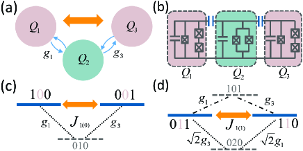
Figure 10: (a) Sketch of a -B-A-B-type system with NN coupling. Dispersive interaction between adjacent qubits (denoted as round arrows) can result in an effective NNN coupling (denoted as double-headed arrows). (b) Circuit diagram of a chain of three superconducting qubits capacitively coupled to each other, where the $Q_{1(3)}$ and $Q_{2}$ are C-shunted flux qubit and transmon qubit, which can be modeled as weak anharmonic oscillators with positive and negative anharmonicity, respectively. (c) For the intermediary qubit $Q_{2}$ in $|0\rangle$ state, the NNN exchange interaction with strength $J_{1(\textbf{0})}$ is enabled by a single path (denoted as dashed lines) involving the intermediate state $|010\rangle$. (d) For $Q_{2}$ in $|1\rangle$ state, the NNN interaction with strength $J_{1(\textbf{1})}$ is enabled by two paths (denoted as dashed lines and dash-dotted lines, respectively), and each involves an intermediate state, i.e.,$|101\rangle$ or $|020\rangle$.

As discussion in Sec. II of the main text, and also according to Eqs. (B5) and (B10) (Eq. (3) in the main text), one can find that in a three-qubit system with NN coupling, when $\alpha_{2}=-\Delta_{1}=-\Delta_{3}$, the two competitive contributions in Eq. (B10) yield zero net coupling strength $J_{1(\textbf{1})}=0$, and the $J_{1(\textbf{0})}$ is preserved. Thus, a switchable NNN coupling can be realized in two concrete settings (Here note that in present work, the A (B) labels qubit with negative (positive) anharmonicity, and a promising implantation is the transmon-CSFQ (C-shunt flux qubit)-transmon system): (1) in an -A-B-A-type setting as shown in Figs. 1(a) and 1(b) , the anharmonicity of $Q_{2}$ (B-type qubit) takes a positive value. Thus, in order to meet the requirement for implementing the switchable NNN coupling, i.e., $\alpha_{2}=-\Delta_{1}=-\Delta_{3}$, the qubit frequency of $Q_{2}$ should satisfy $\tilde{\omega}_{2}>\tilde{\omega}_{j}$. This has been demonstrated in the main text. (2) in a -B-A-B-type setting (CSFQ-transmon-CSFQ) as shown in Figs. 10(a) and 10(b), the anharmonicity of $Q_{2}$ (here is an A-type qubit) takes a negative value. As shown in Fig. 10(d), in order to destructively interfere the two terms in Eq. (B10), the qubit frequency of $Q_{2}$ should satisfy $\tilde{\omega}_{2}<\tilde{\omega}_{j}$. Hence, when $\alpha_{2}=-\Delta_{1}=-\Delta_{3}$, a switchable coupling can also be realized in this setting.

Appendix D Switchable NNN exchange interaction for higher energy levels

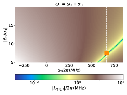
Figure 11: Calculated values of $J_{2(\textbf{1}),I}$ versus $\alpha_{2}$ and $\Delta_{3}$ in the unit of $g_{3}$ with $\omega_{1}=\omega_{3}+\alpha_{3}$. The anharmonicity $\alpha_{j}$ and NN coupling strength $g_{j}$ take the same values as in Fig. 2(b) of the main text. The intersection (orange square) of the vertical cut and the dark strip gives the ideal optimal working point for realizing switchable coupling between $|11\rangle_{1,3}$ and $|02\rangle_{1,3}$ with $\alpha_{2}/2\pi$ take a value of $665\,\rm MHz$.

From the expression in Eqs. (B6) and (B11), one can find that a switchable exchange interaction between qubit state and non-qubit states for $Q_{1}$ and $Q_{3}$, such as the interaction $|11\rangle_{1,3}\leftrightarrow|02\rangle_{1,3}$ with strength $J_{2(\textbf{1}),I}$, can be achieved by engineering the anharmonicity of $Q_{2}$, as shown in Fig. 9. Hence, as same as the case for the virtual exchange interaction in qubit space, this exchange interaction is controlled by the state of $Q_{2}$, i.e., when $Q_{2}$ in $|0\rangle$ state, the interaction is turned on, causing the ZZ interaction between $Q_{1}$ and $Q_{3}$, while for $Q_{2}$ in $|1\rangle$ state, the interaction is turned off.

According to Eq. (B11), Figure  11 shows the calculated $J_{2(\textbf{1}),I}$ versus the anharmonicity $\alpha_{2}$ and qubit detuning $\Delta_{3}$ in the unit of the NN coupling strength $g_{j}$ with $\omega_{1}=\omega_{3}+\alpha_{3}$. The system parameters used are $g_{j}/2\pi=45\,\rm MHz$, and $\alpha_{j}/2\pi=-350\,\rm MHz$. The regime indicated by the darker strip shows the working point, where the interaction $|11\rangle_{1,3}\leftrightarrow|02\rangle_{1,3}$ is turned off, when $Q_{2}$ is in state $|1\rangle$. From the result shown in Fig. 8, one can find that in order to operate in the dispersive regime or quasi-dispersive regime, the value of $\alpha_{2}$ should be larger than $500\,\rm MHz$. For $\alpha_{2}$ taking a value below $500\,\rm MHz$, the dispersive model, as well as the approximation adopted in the present work, may break down. Thus, in the following discussion, $\alpha_{2}$ takes values larger than $500\,\rm MHz$.

Following the same procedure as that for finding the optimal working for implementing C-iSWAP gate, we can also find the optimal working point for realizing switchable coupling between $|11\rangle_{1,3}$ and $|02\rangle_{1,3}$, as shown in Fig. 12. Hence, it is possible to implement the controlled-CZ gate with the switchable coupling between $|11\rangle_{1,3}$ and $|02\rangle_{1,3}$. As shown in Figs. 12(c) and 12(d), a controlled-CZ gate could be implemented in $120\,\rm ns$. Similar result can also be obtained for coupling between $|11\rangle_{1,3}$ and $|20\rangle_{1,3}$. However, for the directly coupled system considered in the present work, only when the magnitudes of anharmonicity of the two adjacent qubits are comparable to each other and have opposite signs, could the residual parasitic ZZ coupling between adjacent qubits be heavily suppressed R14 . Since the anharmonicity of transmon qubit is around $200-400\,\rm MHz$, for the directly coupled system with $\alpha_{2}$ of $665\,\rm MHz$ as shown in Fig. 12, the residual parasitic ZZ coupling between adjacent qubits cannot be heavily suppressed, thus limiting the performance of the controlled-CZ gate. However, for indirectly coupled system, such as a two-qubit system coupled via a bus or a tunable coupler, the residual parasitic ZZ coupling can be heavily suppressed without the requirement that the magnitudes of anharmonicity of the two adjacent qubits are comparable to each other R13 ; R14 .

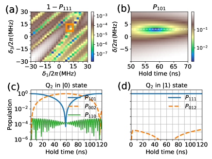
Figure 12: Optimal working point for realizing switchable coupling between $|11\rangle_{1,3}$ and $|02\rangle_{1,3}$ with $\alpha_{2}/2\pi$ taking the value of $665\,\rm MHz$. (a) Swap error $1-P_{111}$ versus the frequency offsets $\delta_{1}$ and $\delta_{3}$ that are defined relative the ideal interaction point, as shown in the inset of Fig. 8. The system is initialized in the eigenstate $|\widetilde{111}\rangle$ at the idle point, and the hold time takes a value of 60 $\rm ns$. The (orange) square indicates the working point where the NNN exchange interaction is turned off for $Q_{2}$ in $|1\rangle$. (b) Population $P_{101}$ versus the overshoot $\delta=\delta_{1}-\delta_{3}$ and the hold time for system initialized in the eigenstate $|\widetilde{101}\rangle$ at the idle point. The horizontal cut (dashed line) depicts the optimal value of overshot for enabling a full complete swap between $|\widetilde{101}\rangle$ and $|\widetilde{002}\rangle$. (c) Population swap $|\widetilde{101}\rangle\Leftrightarrow|\widetilde{002}\rangle$ and (d) $|\widetilde{111}\rangle\Leftrightarrow|\widetilde{012}\rangle$ versus hold time for system initialized in $|\widetilde{101}\rangle$ and $|\widetilde{111}\rangle$, respectively. With optimal frequency offset and overshot obtained from (a) and (b), the NNN exchange interaction $|11\rangle_{1,3}\leftrightarrow|02\rangle_{1,3}$ is turned on or off depending on the state of $Q_{2}$.

Appendix E C-$\rm i$SWAP gate

As mentioned in the main text, in order to implement the C-iSWAP gate in our proposed system, the rounded trapezoid-shaped pulses are applied to adjust the frequency of $Q_{1}$ and $Q_{3}$, thus during the gate implementation, the qubit frequencies vary from the idle point to the interaction point, while the frequency of $Q_{2}$ keeps fixed. The rounded trapezoid-shaped pulse used in present work is described by a time-dependent function R27

$$\omega(t)= \omega_{i}+\frac{\omega_{I}-\omega_{i}}{2}[{\rm Erf}(\frac{t-\frac{t_{\rm ramp}}{2}}{\sqrt{2}\sigma})-{\rm Erf}(\frac{t-t_{\rm g}+\frac{t_{\rm ramp}}{2}}{\sqrt{2}\sigma})]$$ (33)

where $\omega_{i}$ and $\omega_{I}$ denote the idle frequency point (where the logical states are defined as as the eigenstates of the system biased at this point, as discussed in Appendix  A) and the interaction frequency point, respectively, the ramp time is defined as $t_{\rm ramp}=4\sqrt{2}\sigma$ with $\sigma=1\,\rm ns$, $t_{\rm g}$ represents the total time for implementing the gate operation, and the hold time $t_{\rm hold}=t_{\rm g}-t_{\rm ramp}$ is defined as the time-interval between the midpoints of the ramps.

E.1 Intrinsic gate fidelity

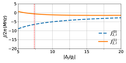
Figure 13: Calculated strength of the effective NNN interaction $|101\rangle\Leftrightarrow|002\rangle$ with $J_{2(\textbf{1}),I}$ and interaction $|111\rangle\Leftrightarrow|012\rangle$ with $J_{2(\textbf{0}),II}$ versus qubit detuning $\Delta_{j}$ ($\Delta_{1}=\Delta_{3}$) in the unit of the NN coupling strength $g_{j}$. The system parameters used are $g_{j}/2\pi=45\,\rm MHz$, $\alpha_{1}/2\pi=\alpha_{3}/2\pi=-350\,\rm MHz$, and $\alpha_{2}/2\pi=350\,\rm MH$. The vertical red dashed line indicates the working point for the implementation of C-iSWAP gate.

To quantify the intrinsic performance of the proposed C-iSWAP gate implementation, the metric of state-average gate fidelity is used in present work. The fidelity is defined as R29

$$F\equiv\frac{{\rm{Tr}}(U^{\dagger}U)+|{\rm{Tr}}(U_{{\rm target}}^{\dagger}U)|^{2}}{72}$$ (34)

where $U$ is the actual evolution operator in the logical eigenbasis at the idle point after applying an auxiliary single-qubit $Z$ rotation on each of the three-qubits before and after the gate implementation, truncated to the qubit levels R27 ; R30 ; R31 , and $U_{\rm target}=U_{CXY}(\pi/2)$ is given as Eq. (5) of the main text.

According to the system Hamiltonian in Eq. (B1), and the control pulse of Eq. (E1), the actual evolution operator in the rotating frame with respect to $H(0)$ is

$$U_{sys}=\mathcal{\hat{T}}\rm{exp}\left(-i\int_{0}^{t_{g}}H_{R}(t)dt\right),$$ (35)

where $H_{R}(t)=e^{iH(0)t}H(t)e^{-iH(0)t}-H(0)$, and $\mathcal{\hat{T}}$ denotes the time-ordering operator. Thus, $U$ in Eq. (E2) is given as

$$U=U_{\rm{post}}\mathcal{P}U_{sys}\mathcal{P}^{\dagger}U_{\rm{pre}},$$ (36)

where $\mathcal{P}$ is the projected operator defined in the computational subspace of the full system, and $U_{\rm{post}}$ and $U_{\rm{pre}}$ are

$$U_{\rm{post}}=e^{-i\phi_{1}ZII/2}e^{-i\phi_{2}IZI/2}e^{-i\phi_{3}IIZ/2},$$ (37)

$$U_{\rm{pre}}=e^{-i\phi^{\prime}_{1}ZII/2}e^{-i\phi^{\prime}_{2}IZI/2}e^{-i\phi^{\prime}_{3}IIZ/2}.$$

Hence, the gate fidelity is obtained as

$$F=\rm{maximize}_{\phi_{j},\phi^{\prime}_{j}}\,\,F(\phi_{j},\phi^{\prime}_{j}),$$ (38)

taking a value of $99.97\%$ for $t_{\rm hold}=43\,\rm ns$. Aside from the control error (as shown in Fig. 4(a)) and leakage to non-qubit states (as shown in Fig. 4(b)), the residual infidelity is caused by the coherence phase resulting from ZZ interaction between qubits, as shown in the effective Hamiltonian of Eq. (B14). Hence, by assuming no control error and leakage, the actual implemented unitary operator can be described by

$$U=\left(\begin{array}[]{cccccccc}1&0&0&0&0&0&0&0\\ 0&0&0&0&-i&0&0&0\\ 0&0&1&0&0&0&0&0\\ 0&0&0&e^{-i\phi_{011}}&0&0&0&0\\ 0&-i&0&0&0&0&0&0\\ 0&0&0&0&0&e^{-i\phi_{101}}&0&0\\ 0&0&0&0&0&0&e^{-i\phi_{110}}&0\\ 0&0&0&0&0&0&0&e^{-i\phi_{111}}\\ \end{array}\right),$$ (39)

where $\phi_{s}$ ($\rm s=011,\,101,\,110,\,111$) represents the accumulated phase caused by the ZZ interaction during the gate operation.

In Table $\rm II$ of the main text, we have also shown the accumulated phase caused by the ZZ interaction between qubits during the gate implementation, defined as

$$\phi_{s}=\rm{arg}\left(\langle s|U|s\rangle\right),$$ (40)

i.e, the argument of the matrix element $U_{ss}=\langle s|U|s\rangle$. Strikingly, in Table $\rm II$, one can find that the accumulated phase in state $|101\rangle$ takes the largest value $0.01728$, while in state $|111\rangle$, it is below $0.01$. This is caused by the fact that, as shown in Fig. 5, similar to the exchange interaction in qubit space $\{|100\rangle,\,|001\rangle\}$ and $\{|110\rangle,\,|011\rangle\}$, the strength of the virtual exchange interactions between qubit states and non-qubit states also depends on the state of $Q_{2}$, thus enabling the ZZ interaction (accumulated phase) to be controlled by the state of $Q_{2}$. As shown in Fig. 13, one can find that at the interaction point (indicated as the red dashed line), the strength of the interactions between qubit states and non-qubit states ($|101\rangle\Leftrightarrow|002\rangle$) $J_{2(\textbf{0}),I}$ is larger than that of the interaction $|111\rangle\Leftrightarrow|012\rangle$. Similar result can also be obtained for the interaction $|101\rangle\Leftrightarrow|200\rangle$ and the interaction $|111\rangle\Leftrightarrow|210\rangle$. This could explain the striking feature in Table $\rm II$.

E.2 Gate operation with the typical coupling strength

Figure 14: The intrinsic gate fidelity versus the anharmonicity $\alpha_{2}$ and hold time with $g_{j}/2\pi=30\,\rm MHz$. Other system parameters used here are the same as the parameters listed in Table $\rm I$.

As mentioned in the main text, although the implementation of the native three-qubit gates may benefit from the strong fixed coupling between adjacent qubits, this strong coupling may make single qubit addressing R35 and the implementation of two-qubit gates R4 ; R34 a challenge for system with limited frequency tunability. However, as shown in Fig. 14, with NN coupling strength of $30\,\rm MHz$ R4 and fixed ramp time $t_{\rm ramp}=4\sqrt{2}\,\rm ns$, the intrinsic gate fidelity above $99\%$ ($99.9\%$) can still be achieved in 50 (100) $\rm ns$. We note that choosing larger ramp time, thus lengthening the gate time, should further reduce the leakage error R28 ; R33 . Therefore, the intrinsic gate fidelity could further be improved at the expense of increased gate time.

E.3 Decoherence effect

To evaluate the impact of decoherence process on the implemented gate performance, we analyze the full system dynamics according to the Lindblad master equation

$$\dot{\rho}(t)=-i[H,\rho(t)]+\sum_{l}\left(\frac{1}{T_{1}}\mathcal{C}[q_{l}]+\frac{2}{T_{\phi}}\mathcal{C}[q_{l}^{{\dagger}}q_{l}]\right)$$ (41)

where $H$ is the system Hamiltonian given in Eq. (1), $\rho$ is the reduced density matrix of the system, and $\mathcal{C}[O]=O\rho(t)O^{{\dagger}}-\frac{1}{2}\{O^{{\dagger}}O,\rho(t)\}$. In the Liouvile space R42 ; R43 , a ($n\times n$) density matrix $\rho$ in Hilbert space can be mapped as a ($n^{2}\times 1$) vector $|\rho\rangle\rangle$, and a target unitary operator $U_{\rm target}$ ($n\times n$) in Hilbert space can be mapped to a superoperator $\mathcal{P}_{U_{\rm target}}=U^{\ast}_{\rm target}\otimes U_{\rm target}$ ($n^{2}\times n^{2}$). Thus, in the Liouvile space, Eq. (E9) can be rewritten as (assuming $T_{\phi}=\infty$, thus ignoring the dephasing term $\mathcal{L}[q_{l}^{{\dagger}}q_{l}]$) R42 ; R43

$$\frac{d|\rho\rangle\rangle}{dt}= \mathcal{L}_{t}|\rho\rangle\rangle=\left[-i(I\otimes H-H^{T}\otimes I)\right]|\rho\rangle\rangle+$$ (42)

$$\sum_{l}\left[q_{l}^{\ast}\otimes q_{l}-\frac{1}{2}I\otimes q_{l}^{{\dagger}}q_{l}-\frac{1}{2}q_{l}^{T}q_{l}^{\ast}\otimes I\right]|\rho\rangle\rangle,$$

where $\ast$ denotes the complex conjugate, $T$ means the matrix transpose, $\otimes$ the Kronecker product, and $I$ is the identity operator. Thus, the time-evolution superoperator is given as $\mathcal{P}_{U}=\mathcal{\hat{T}}{\rm{exp}}\left(\int_{0}^{t_{g}}\mathcal{L}_{t}dt\right)$.

Based on the about discussion, the average gate fidelity $F_{o}$ between target $U_{\rm target}$ and the actually implemented operation under decoherence process is defined as R29 ; R39 ; R40 ; R41

$$\begin{aligned} F_{o}=\frac{8(1-L_{1})+{\rm Tr}(\mathcal{P}_{U}^{{\dagger}}\mathcal{P}_{U_{\rm{target}}})}{72},\end{aligned}$$ (43)

with $L_{1}$ denotes the leakage of the gate operation, given as R39 ; R40

$$\begin{aligned} L_{1}=1-\frac{1}{8}\sum_{i,j,k\in\{0,1\}}{\rm Tr}(\mathcal{P}_{U}|ijk\rangle\rangle),\end{aligned}$$ (44)

where $|ijk\rangle\rangle$ denotes the logical qubit state $|ijk\rangle$ represented in the Liouville space.

Similarly, we can also give the idling gate fidelity for single qubit by assuming only $T_{1}$ and $T_{\phi}$ decay process R29 , i.e,

$$F_{I} =\frac{\rm{Tr}(\sum_{k}M_{k}^{{\dagger}}M_{k})+\sum_{k}|\rm{Tr}(M_{k})|^{2}}{6}$$ (45)

$$=\frac{3+e^{-t/T_{1}}+2e^{-t(1/2T_{1}+1/T_{\phi})}}{6}$$

$$\approx 1-\frac{t}{3T_{1}}-\frac{t}{3T_{\phi}},$$

where $M_{k}$ denotes the Kraus operator describing the decoherence effect on the qubit state, i.e., $\Lambda_{T_{1},T_{\phi}}(\rho)=\sum_{k}M_{k}\rho M_{k}^{{\dagger}}$ with $\sum_{k}M_{k}^{{\dagger}}M_{k}=I$. The term $\mathcal{C}[O]$ in Eq. (E9) resulting from decoherence process can be derived from the following three Kraus operators R19 ; R29 ; R55 ,

$$M_{0}=\left(\begin{array}[]{cc}1&0\\ 0&\sqrt{1-\lambda-\gamma}\\ \end{array}\right)$$ (46)

$$M_{1}=\left(\begin{array}[]{cc}0&0\\ 0&\sqrt{\lambda}\\ \end{array}\right),$$ (47)

$$M_{2}=\left(\begin{array}[]{cc}0&\sqrt{\gamma}\\ 0&0\\ \end{array}\right),$$ (48)

where

$$\lambda=e^{-t/T_{1}}(1-e^{-2t/T_{\phi}}),$$ (49)

$$\gamma=1-e^{-t/T_{1}}.$$

with $T_{1}$ ($T_{\phi}$) denotes the qubit energy relaxation time (qubit dephasing time). For our proposed three-qubit system, the idling gate fidelity can be approximated as $F=F_{I}^{3}$.

References

- (1) A. G. Fowler, M. Mariantoni, J. M. Martinis, and A. N. Cleland, Surface codes: Towards practical large-scale quantum computation, Phys. Rev. A 86, 032324 (2012).
- (2) B. R. Johnson. Controlling Photons in Superconducting Electrical Circuits. PhD thesis, Yale University, May 2011.
- (3) A. Galiautdinov, A. N. Korotkov, and J. M. Martinis, Resonator-zero-qubit architecture for superconducting qubits, Phys. Rev. A 85, 042321 (2012).
- (4) R. Barends, J. Kelly, A. Megrant, A. Veitia, D. Sank, E. Jeffrey, T. C. White, J. Mutus, A. G. Fowler, B. Campbell, Y. Chen, Z. Chen, B. Chiaro, A. Dunsworth, C. Neill, P. O’Malley, P. Roushan, A. Vainsencher, J. Wenner, A. N. Korotkov, A. N. Cleland, and J. M. Martinis, Superconducting quantum circuits at the surface code threshold for fault tolerance, Nature 508, 500 (2014).
- (5) F. Yan, P. Krantz, Y. Sung, M. Kjaergaard, D. L. Campbell, T. P. Orlando, S. Gustavsson, and W. D. Oliver, Tunable Coupling Scheme for Implementing High-Fidelity Two-Qubit Gates, Phys. Rev. Applied 10, 054062 (2018).
- (6) J. Preskill, Quantum Computing in the NISQ era and beyond, Quantum 2, 79 (2018).
- (7) M. Roth, M. Ganzhorn, N. Moll, S. Filipp, G. Salis, and S. Schmidt, Analysis of a parametrically driven exchange-type gate and a two-photon excitation gate between superconducting qubit, Phys. Rev. A 96, 062323 (2017).
- (8) F. W. Strauch, P. R. Johnson, A. J. Dragt, C. J. Lobb, J. R. Anderson, and F. C. Wellstood, Quantum Logic Gates for Coupled Superconducting Phase Qubits, Phys. Rev. Lett. 91, 167005 (2003).
- (9) L. DiCarlo, J. M. Chow, J. M. Gambetta, L. S. Bishop, B. R. Johnson, D. I. Schuster, J. Majer, A. Blais, L. Frunzio, S. M. Girvin, and R. J. Schoelkopf, Demonstration of two-qubit algorithms with a superconducting quantum processor, Nature(London) 460, 240 (2009).
- (10) D. C. McKay, S. Filipp, A. Mezzacapo, E. Magesan, J. M. Chow, and J. M. Gambetta, Universal gate for fixed-frequency qubits via a tunable bus, Phys. Rev. Applied 6, 064007 (2016).
- (11) M. Roth, N. Moll, G. Salis, M. Ganzhorn, D. J. Egger, S. Filipp, and S. Schmidt, Adiabatic quantum simulations with driven superconducting qubits, Phys. Rev. A 99, 022323 (2019).
- (12) M. Ganzhorn, D.J. Egger, P. Barkoutsos, P. Ollitrault, G. Salis, N. Moll, M. Roth, A. Fuhrer, P. Mueller, S. Woerner, I. Tavernelli, and S. Filipp, Gate-Efficient Simulation of Molecular Eigenstates on a Quantum Computer, Phys. Rev. Applied 11, 044092 (2019).
- (13) J. Ku, X. Xu, M. Brink, D. C. McKay, J. B. Hertzberg, M. H. Ansari, and B.L.T. Plourde, Suppression of Unwanted ZZ Interactions in a Hybrid Two-Qubit System, arXiv:2003.02775.
- (14) P. Zhao, P. Xu, D. Lan, J. Chu, X. Tan, H. Yu, and Y. Yu, High-contrast ZZ interaction using multi-type superconducting qubits, arXiv:2002.07560.
- (15) H. C. J. Gan, G. Maslennikov, Ko-Wei Tseng, C. Nguyen, and D. Matsukevich, Hybrid quantum computation gate with trapped ion system, arXiv:1908.10117.
- (16) N. J. S. Loft, M. Kjaergaard, L. B. Kristensen, C. K. Andersen, T. W. Larsen, S. Gustavsson, W. D. Oliver, and N. T. Zinner, Quantum interference device for controlled two-qubit operations, arXiv:1809.09049.
- (17) P. J. Liebermann, P.-L. Dallaire-Demers, F. K. Wilhelm, Implementation of the iFREDKIN gate in scalable superconducting architecture for the quantum simulation of Fermionic systems, arXiv:1701.07870.
- (18) S. E. Rasmussen, and N. T. Zinner, Simple implementation of high fidelity controlled-iSWAP gates and quantum circuit exponentiation of non-Hermitian gates, arXiv:2002.11728.
- (19) M. A. Nielsen and I. L. Chuang, Quantum Computation and Quantum Information (Cambridge University Press, Cambridge UK, 2010).
- (20) P. J. J. O’Malley, R. Babbush, I. D. Kivlichan, J. Romero, J. R. McClean, R. Barends, J. Kelly, P. Roushan, A. Tranter, N. Ding, B. Campbell, Y. Chen, Z. Chen, B. Chiaro, A. Dunsworth, A. G. Fowler, E. Jeffrey, A. Megrant, J. Y. Mutus, C. Neill, C. Quintana, D. Sank, A. Vainsencher, J. Wenner, T. C. White, P. V. Coveney, P. J. Love, H. Neven, A. Aspuru-Guzik, and J. M. Martinis, Scalable Quantum Simulation of Molecular Energies, Phys. Rev. X 6, 031007 (2016).
- (21) J. Koch, T. M. Yu, J. Gambetta, A. A. Houck, D. I. Schuster, J. Majer, A. Blais, M. H. Devoret, S. M. Girvin, and R. J. Schoelkopf, Charge-insensitive qubit design derived from the cooper pair box, Phys. Rev. A 76, 042319 (2007).
- (22) J. Q. You, X. Hu, S. Ashhab, and F. Nori, Low-decoherence flux qubit, Phys. Rev. B 75, 140515(R) (2007).
- (23) M. Steffen, S. Kumar, D. P. DiVincenzo, J. R. Rozen, G. A. Keefe, M. B. Rothwell, and M. B. Ketchen, High-Coherence Hybrid Superconducting Qubit, Phys. Rev. Lett. 105, 100502 (2010).
- (24) F. Yan, S. Gustavsson, A. Kamal, J. Birenbaum, A. P. Sears, D. Hover, T. J. Gudmundsen, D. Rosenberg, G. Samach, S. Weber, J. L. Yoder, T. P. Orlando, J. Clarke, A. J. Kerman, and W. D. Oliver, The flux qubit revisited to enhance coherence and reproducibility, Nat. Commun. 7, 12964 (2016).
- (25) S. Bravyi, D. P. DiVincenzo, and D. Loss, Schrieffer-Wolff transformation for quantum many-body systems, Ann. Phys 326, 2793 (2011).
- (26) S. Poletto, J. M. Gambetta, S. T. Merkel, J. A. Smolin, J. M. Chow, A. D. Córcoles, G. A. Keefe, M. B. Rothwell, J. R. Rozen, D. W. Abraham, C. Rigetti, and M. Steffen, Entanglement of Two Superconducting Qubits in a Waveguide Cavity via Monochromatic Two-Photon Excitation, Phys. Rev. Lett. 109, 240505 (2012).
- (27) J. Ghosh, A. Galiautdinov, Z. Zhou, A. N. Korotkov, J. M. Martinis, and M. R. Geller, High-fidelity controlled- gate for resonator-based superconducting quantum computers, Phys. Rev. A 87, 022309 (2013).
- (28) R. Barends, C. M. Quintana, A. G. Petukhov, Y. Chen, D. Kafri, K. Kechedzhi et al., Diabatic Gates for Frequency-Tunable Superconducting Qubits, Phys. Rev. Lett. 123, 210501 (2019).
- (29) L. H. Pedersen, N. M. Møller, and K. Mølmer, Fidelity of quantum operations, Phys. Lett. A 367, 47 (2007).
- (30) E. Zahedinejad, J. Ghosh, and B. C. Sanders, Designing High-Fidelity Single-Shot Three-Qubit Gates: A Machine-Learning Approach, Phys. Rev. Applied 6, 054005 (2016).
- (31) E. Barnes, C. Arenz, A. Pitchford, and S. E. Economou, Fast microwave-driven three-qubit gates for cavity-coupled superconducting qubits, Phys. Rev. B 96, 024504 (2017).
- (32) B. Foxen, C. Neill, A. Dunsworth, P. Roushan, B. Chiaro et al., Demonstrating a Continuous Set of Two-qubit Gates for Near-term Quantum Algorithms, arXiv:2001.08343.
- (33) F. Arute, K. Arya, R. Babbush, D. Bacon, J. C. Bardin, R. Barends, R. Biswas, S. Boixo, F. G. Brandao, D. A. Buell, et al., Quantum supremacy using a programmable superconducting processor, Nature 574, 505 (2019).
- (34) J. Kelly, R. Barends, A. G. Fowler, A. Megrant, E. Jeffrey, T. C. White, D. Sank, J. Y. Mutus, B. Campbell, Yu Chen, Z. Chen, B. Chiaro, A. Dunsworth, I.-C. Hoi, C. Neill, P. O’Malley, C. Quintana, P. Roushan, A. Vainsencher, J. Wenner, A. N. Cleland, and J. M. Martinis, State preservation by repetitive error detection in a superconducting quantum circuit, Nature 519, 66 (2015).
- (35) J. M. Gambetta, A. D. Córcoles, S. T. Merkel, B. R. Johnson, J. A. Smolin, J. M. Chow, C. A. Ryan, C. Rigetti, S. Poletto, T. A. Ohki, M. B. Ketchen, and M. Steffen, Characterization of Addressability by Simultaneous Randomized Benchmarking, Phys. Rev. Lett. 109, 240504 (2012).
- (36) Y. Chen, C. Neill, P. Roushan, N. Leung, M. Fang, R. Barends, J. Kelly, B. Campbell, Z. Chen, B. Chiaro, A. Dunsworth, E. Jeffrey, A. Megrant, J. Y. Mutus, P. J. J. O’Malley, C. M. Quintana, D. Sank, A. Vainsencher, J. Wenner, T. C. White, M. R. Geller, A. N. Cleland, and J. M. Martinis, Qubit architecture with high coherence and fast tunable coupling, Phys. Rev. Lett. 113, 220502 (2014).
- (37) C. Neill. A path towards quantum supremacy with superconducting qubits. PhD thesis, University of California Santa Barbara, Dec 2017.
- (38) P. S. Mundada, G. Zhang, T. Hazard, and A. A. Houck, Suppression of Qubit Crosstalk in a Tunable Coupling Superconducting Circuit, Phys. Rev. Applied 12, 054023 (2019).
- (39) C. J. Wood and J. M. Gambetta, Quantification and characterization of leakage errors, Phys. Rev. A 97, 032306 (2018).
- (40) M. A. Rol, F. Battistel, F. K. Malinowski, C. C. Bultink, B. M. Tarasinski, R. Vollmer, N. Haider, N. Muthusubramanian, A. Bruno, B. M. Terhal, and L. DiCarlo, Fast, High-Fidelity Conditional-Phase Gate Exploiting Leakage Interference in Weakly Anharmonic Superconducting Qubits, Phys. Rev. Lett. 123, 120502 (2019).
- (41) M. Abdelhafez, B. Baker, A. Gyenis, P. Mundada, A. A. Houck, D. Schuster, and J. Koch, Universal gates for protected superconducting qubits using optimal control, Phys. Rev. A 101, 022321 (2020).
- (42) C. Navarrete-Benlloch, Open systems dynamics: Simulating master equations in the computer, arXiv:1504.05266.
- (43) T. F. Havel, Robust procedures for converting among Lindblad, Kraus and matrix representations of quantum dynamical semigroups, Journal of Mathematical Physics 44, 534 (2003).
- (44) T. E. Obrien, B. Tarasinski, and L. DiCarlo, Density-Matrix Simulation of Small Surface Codes under Current and Projected Experimental Noise, npj Quantum Inf. 3, 39 (2017).
- (45) N. Schuch and J. Siewert, Natural two-qubit gate for quantum computation using the XY interaction, Phys. Rev. A 67, 032301 (2003).
- (46) T. Roy, S. Hazra, S. Kundu, M. Chand, M. P. Patankar, and R. Vijay, Programmable Superconducting Processor with Native Three-Qubit Gates, Phys. Rev. Applied 14, 014072 (2020).
- (47) S. Daraeizadeh, S. P. Premaratne, N. Khammassi, X. Song, M. Perkowski, and A. Y. Matsuura, Machine-learning-based three-qubit gate design for the Toffoli gate and parity check in transmon systems, Phys. Rev. A 102, 012601 (2020).
- (48) D. M. Abrams, N. Didier, B. R. Johnson, M. P. d. Silva, and C. A. Ryan, Implementation of the XY interaction family with calibration of a single pulse, arXiv:1912.04424.
- (49) R. C. Bialczak, M. Ansmann, M. Hofheinz, E. Lucero, M. Neeley, A. D. ÓConnell, D. Sank, H. Wang, J. Wenner, M. Steffen, A. N. Cleland and J. M. Martinis, Quantum process tomography of a universal entangling gate implemented with Josephson phase qubits, Nature Physics 6, 409 (2010).
- (50) P.-L. Dallaire-Demers and F. K. Wilhelm, Quantum gates and architecture for the quantum simulation of the Fermi-Hubbard model, Phys. Rev. A 94, 062304 (2016).
- (51) J. Kelly, R. Barends, B. Campbell, Y. Chen, Z. Chen, B. Chiaro, A. Dunsworth, A. G. Fowler, I.-C. Hoi, E. Jeffrey, A. Megrant, J. Mutus, C. Neill, P. J. J. ÓMalley, C. Quintana, P. Roushan, D. Sank, A. Vainsencher, J. Wenner, T. C. White, A. N. Cleland, and J. M. Martinis, Optimal Quantum Control Using Randomized Benchmarking, Phys. Rev. Lett. 112, 240504 (2014).
- (52) D. J. Egger and F. K. Wilhelm, Adaptive Hybrid Optimal Quantum Control for Imprecisely Characterized Systems, Phys. Rev. Lett. 112, 240503 (2014).
- (53) S. Machnes, E. Assémat, D. Tannor, and F. K. Wilhelm, Tunable, Flexible, and Efficient Optimization of Control Pulses for Practical Qubits, Phys. Rev. Lett. 120, 150401 (2018).
- (54) J. D. Whitfield, J. Biamonte, and A. Aspuru-Guzik, Simulation of Electronic Structure Hamiltonians Using Quantum Computers, Mol. Phys. 109, 735 (2011).
- (55) D. C. McKay, S. Sheldon, J. A. Smolin, J. M. Chow, and J. M. Gambetta, Three Qubit Randomized Benchmarking, Phys. Rev. Lett. 122, 200502 (2019).