Seeing the Forest for the Trees: Scaling Analysis of Energy in Great Lakes Water Supplies

ORCID: 0000-0002-7183-1157

Version: October 3, 2019

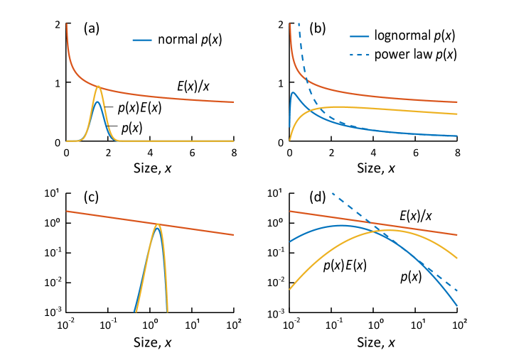
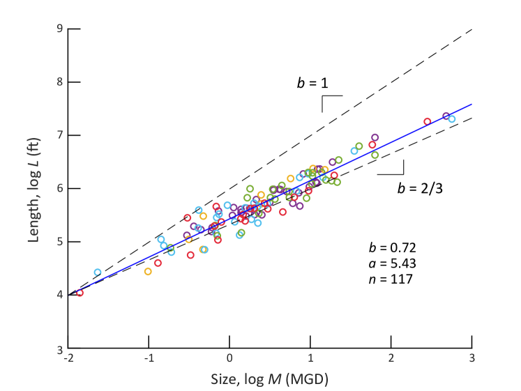
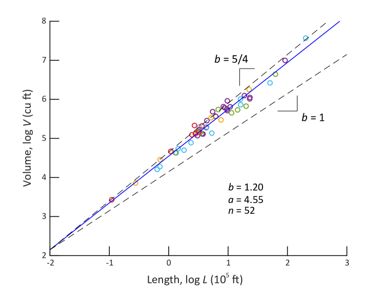
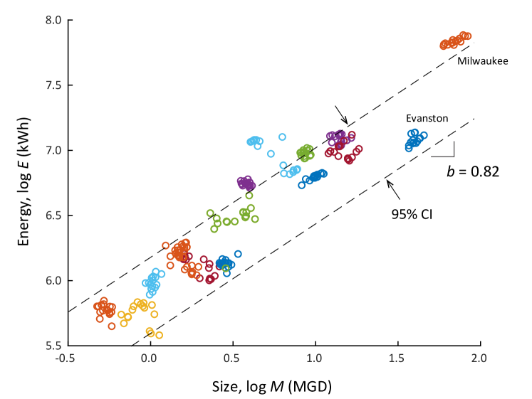
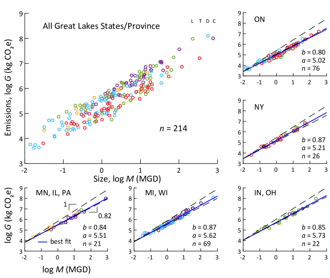
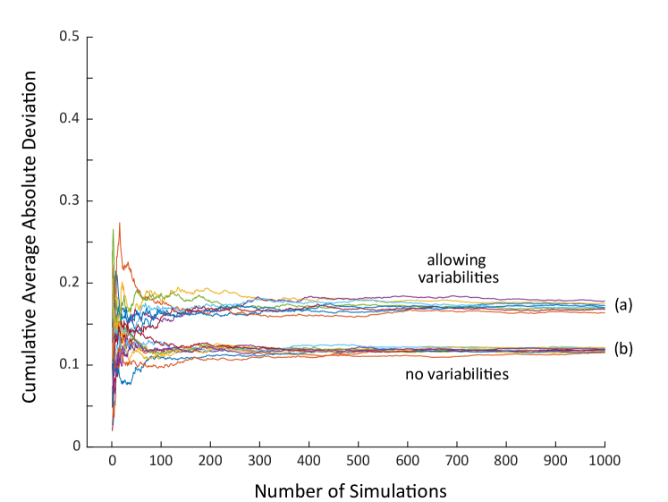
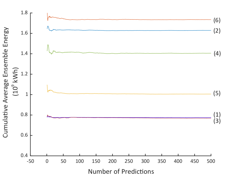
Figure 1: Comparison between (a,c) the normal distribution and (b,d) the lognormal and power-law distributions of a random size variable $x$, shown in (a,b) linear-linear space and (c,d) log-log space, respectively. $p(x)$ (blue) is the probability density function of the normal (SD, 0.3), lognormal ($\sigma=1.5$), and power-law ($\alpha=1.1$) distributions, respectively; $E(x)/x$ (red) is the energy intensity function, where $E(x)$ is the allometric energy function ($b=0.8$); and $p(x)E(x)$ (yellow) is the ensemble energy at size $x$. For the normal distribution, $p(x)$ is exponentially “bounded”. A randomly selected $x$ falls within a narrow range of the ensemble mean $\bar{x}$ because the standard deviation is of the same scale as the mean ¹. The bounded nature of the normal distribution allows $\bar{x}$ to be used as an approximation for the PDF and $p(x)E(x)\sim p(\bar{x})E(\bar{x})$ is insensitive to the variation of $E(x)$. Thus, the evaluation of the ensemble energy can be simplified to random sampling because of the convergence of the sampled $x$ to $\bar{x}$. For a power-law or power-law-tailed lognormal distribution, $p(x)$ is “unbounded”. A randomly sampled $x$ can be arbitrarily large because the standard deviation of the power-law distribution is divergent ¹. The unbounded nature of the power-law implies that there is no typical $x$ sampling can capture. The evaluation of $p(x)E(x)$ must be done by analytically integrating $E(x)$ over $p(x)$, or by numerically summing $E(x)$ for all $x$, because $E(x)$ is a transscale nonlinear (power-law) function in itself.

Figure 2: Scaling of network length $L$ with size $M$ for selected Great Lake communities that host a supply system², with linear best-fit (blue line). Black dashed-lines indicate theoretical scaling ($b=\frac{2}{3}$) and isometric scaling ($b=1$), respectively. Data points are color-coded by lake as indicated in Figure 4 in the main text. The logarithm is 10-based.

Figure 3: Scaling of network volume $V$ with network length $L$ for selected Great Lake communities that host a supply system², with linear best-fit (blue line). Black dashed-lines indicate theoretical scaling ($b=\frac{5}{4}$) and isometric scaling ($b=1$), respectively.

Figure 4: Scaling of system energy (electricity) with system size as time series for 15 available supply systems (each shown in a distinct color) and for a period of 20 years (1997-2016). Dashed-lines indicate the 95% confidence interval of the residual distribution from the fitted line for energy scaling, representing “inter-system variations” (SD, 0.15). An “intra-system variation” (SD, 0.05) is calculated from the vertical variations of each individual system then averaged over all systems. The data are drawn from the systems at Ashland³, Superior⁴, Cudahy⁵, Green Bay ⁶, Kenosha⁷, Manitowoc⁸, Marinette⁹, Milwaukee¹⁰, Oak Creek¹¹, Port Washington¹², Racine¹³, Sheboygan¹⁴,South Milwaukee¹⁵, Two Rivers¹⁶, and Evanston¹⁷.

Figure 5: Allometric GHG emission scaling in SSs. Predicted annual GHG emissions $G$ (circles; color-coded by lake) associated with electricity use are plotted against system size $M$ in log-log space for the all-Great Lakes dataset and for individual or similar jurisdictions datasets.

Figure 6: Cumulative average absolute difference in log space between empirical and predicted individual system energies for randomly selected individual systems (a) with and (b) without variabilities. Multiple traces are shown.

Figure 7: Cumulative averages of ensemble energies (trace numbers correspond to peak numbers in Figure 5b,d,f) (1) empirical SS ensemble energy excluding the largest six systems; (2) empirical SS ensemble energy including all systems; (3) predicted SS ensemble energy excluding the largest six systems; (4) predicted SS ensemble energy including all systems; (5) predicted CC ensemble energy excluding CCs served by the largest six systems; and (6) predicted CC ensemble energy including all systems.