A Real-Time Balancing Market Optimization with Personalized Prices: From Bilevel to Convex

Abstract

This paper studies the static economic optimization problem of a system with a single aggregator and multiple prosumers in a *rtbm. The aggregator, as the agent responsible for portfolio balancing, needs to minimize the cost for imbalance satisfaction in real-time by proposing a set of optimal personalized prices to the prosumers. On the other hand, the prosumers, as price taker and self-interested agents, want to maximize their profit by changing their supplies or demands and providing flexibility based on the proposed personalized prices. We model this problem as a bilevel optimization problem. We first show that the optimal solution of this bilevel optimization problem can be found by solving an equivalent convex problem. In contrast to the state-of-the-art *mip-based approach to solve bilevel problems, this convex equivalent has very low computation time and is appropriate for real-time applications. Next, we compare the optimal solutions of the proposed personalized scheme and a uniform pricing scheme. We prove that, under the personalized pricing scheme, more prosumers contribute to the rtbm and the aggregator’s cost is less. Finally, we verify the analytical results of this work by means of numerical case studies and simulations.

mip short = MIP , long = Mixed-Integer Programming , sort = M , der short = DER , long = Distributed Energy Resources , sort = D , rtbm short = RTBM , long = Real-Time Balancing Market , sort = R , ads short = ADS , long = Active Demand and Supply , sort = A , brp short = BRP , long = Balance Responsible Party , sort = B , tso short = TSO , long = Transmission System Operator , sort = T , hp short = HP , long = Heat Pump , sort = H , mchp short = mCHP , long = Micro Combined Heat and Power , sort = m , mpec short = MPEC , long = Mathematical Programming with Equilibrium Constraints , sort = M ,

1 Introduction

In recent years, the increase in the penetration of ders at the demand side has drastically changed the structure of our power system. As a result, the old passive households, which only consumed energy, found a more active role with the help of the demand side generation. The new term prosumer was introduced in the energy community to represent this transition for households [1].

The emergence of prosumers calls for a new real-time market structure in contrast to the existing day ahead and intraday markets. Since output power of many ders is volatile due to their intrinsic environmental dependency, planning for supply and demand matching needs to be done as close as possible to real-time to keep the system stable and economically efficient. Therefore, a rtbm [2] that incorporates available unused capacity of prosumers’ controllable ders and flexible loads, which together we denote here as controllable ads units, should be developed to address the supply volatility by incentivizing prosumers.

Currently, there is only an ex-post financial settlement procedure in the Netherlands and most of Europe, and no actual or physical real-time balancing occurs [3]. Communication infrastructure in the new paradigm of smart grid [4] facilitates the participation of the prosumers with controllable ads units in an rtbm. Moreover, to prevent direct interaction of the prosumers with higher level agents in the market and aggregate them, a market participant, the aggregator, has been introduced [5]. The aggregators have different roles in different market structures.

The goal of an aggregator in an rtbm is to optimize its operational costs for balancing by incentivizing the prosumers to utilize their unused assets. There are many approaches which an aggregator can employ to steer its associated prosumers to an optimal operation point [6]. One of the most popular approaches is to consider the aggregator as a leader, who can anticipate the reaction of the prosumers, proposes some prices to the following prosumers such that their reactions would be optimal for the aggregator. This price incentive oriented setup falls into the category of bilevel optimization problems [7] and Stackelberg games [8], where the lower level problems and the upper level problem are the problems related to the prosumers and the aggregator, respectively.

The bilevel and Stackelberg game modeling of the aggregator and prosumers’ interactions have been studied extensively in the literature [9, 10, 11, 12, 13, 14, 15]. Two different pricing schemes have been proposed to incentivize prosumers in the aforementioned studies. The uniform pricing scheme is an incentivization scheme where the aggregator proposes the same price to all of the prosumers [9, 10]. In the other pricing, i.e., the personalized pricing scheme, the aggregator proposes a unique price to each prosumer in order to reach its goal [16, 12, 13]. While these two pricing schemes have been considered in different works interchangeably and it is argued that the personalized pricing scheme has some benefits over uniform pricing scheme, there exists no research which provides rigorous mathematical proofs on the differences between these two schemes.

Moreover, the state-of-the-art approach to solve these types of bilevel optimization problems is to solve them as mips [9, 17, 18]. However, implementing the mentioned setup in real-time requires very fast computations. The time intervals for a real-time balancing market can often be as low as $5$ minutes [19]. Therefore, the solution for each interval has to be computed and executed within seconds or even less. While papers like [20] have studied the computational efficiency of the bilevel optimization correspond to generating firms strategic offering by introducing a convex relaxation, to the best of our knowledge, no study addressed the computation time for the prosumers/aggregator setup with personalized prices for a high number of prosumers. It should be noted that, although the algorithms in [14] and [16] are distributed, their efficiency are not guaranteed for large problems and real-time applications.

In contrast to the above works, here we stick to a simple model for the aggregator and prosumers interaction with personalized pricing scheme to analyse the corresponding bilevel optimization problem in a fundamental and tractable mathematical way. Although our model is simple, we keep the essence of these market models and most of the results in this paper can be generalized to more complicated and realistic models.

Contributions: We present a bilevel optimization problem to model the interactions between self-interested aggregator and prosumers in an rtbm. A personalized pricing scheme by the aggregator is proposed to incentivize the prosumers to participate in this market. Bilevel problems, in general, are non-convex [21]. We first prove that the global optimal solution of this bilevel optimization problem can be found by solving a convex equivalent problem. This convex equivalent formulation has two main advantages. On the one hand, it guarantees global optimality. On the other hand, a convex formulation is attractive in real-time applications with high number of prosumers since the other approaches to solve bilevel optimization problems (e.g., mip-based approach) are not computationally efficient. Afterwards, we compare the optimal solution of the proposed model with personalized prices to a uniform pricing scheme. We prove that the personalized pricing scheme leads to a less cost for the aggregator and under this pricing scheme more prosumers contribute to the balancing market. Preliminary results of this work are partially presented in the extended abstract [22]. In contrast to the abstract, this paper considers a more general model for the prosumer and provides theoretical proofs for the results. Also, in this paper we compare uniform and personalized pricing schemes in different aspects.

The paper is organized as follows. Section 2 explains the prosumers/aggregator interaction model in a real-time balancing market and introduces the bilevel problem. In Section 3, we show that the bilevel optimization problem is equivalent to a certain convex problem. The analytical comparison of the optimal solution of the proposed personalized pricing scheme and a uniform pricing scheme is presented in Section 4. The efficiency of the proposed method is illustrated by means of simulations in Section 5. Section 6 concludes the paper. The proofs of some theoretical results are presented in A.

2 Problem formulation

In this section, we formulate the static bilevel economic optimization problem of an aggregator and its portfolio for participation in an rtbm. While this paper is devoted to investigate a single time-step, the proposed scheme can also be applied for dynamic cases with multiple time-steps. The general structure of this market is as follows. Each aggregator has a set of prosumers under contract and each prosumer is on a contract with only one aggregator. There are many types of aggregators in an electricity market. In this paper, we consider a commercial aggregator which also acts as a brp [23]. Therefore, the aggregator here is also responsible for balancing its portfolio. To do so, the aggregator receives a real-time price from the tso, who usually has the highest role in the market hierarchy, and incentivizes the prosumers with personalized prices to supply or consume more or less based on that. The change in each prosumer electrical energy supply or demand in a time interval is referred as flexibility. Next, we explain the problem setting and market structure in detail.

Prosumers are equipped with various kinds of ads units. They consist of two prominent categories, namely controllable and uncontrollable units. mchp units and hp units are examples of controllable active supply and demand units of electricity, respectively. Output generation of units such as solar cells and wind turbines is dependent on environmental conditions. Thus these are uncontrollable supply units. Throughout this paper, we assume that each prosumer has a modular mchp and hp as its controllable ads units and it might have a solar panel or wind turbine as an uncontrollable one. Each prosumer heat demand is also assumed to be flexible by considering a loss of comfort factor, that is, it is willing to consume more or less heat if its loss of comfort is compensated by the aggregator. Since heat is an output for both mchp and hp, prosumers are able to alter their controllable ads units output level to participate in the balancing market.

Due to the uncertain nature and volatility of both the uncontrollable ders and the prosumers demand, there could be a mismatch between the pre-planned supply and demand schedules in the real-time. To balance this mismatch and to participate in the rtbm, the aggregator incentivizes the prosumers with personalized prices [24] in a centralized way to consume or supply more energy using their controllable ads units. Before providing a precise mathematical formulation, we elaborate on some technical notions.

The aggregator is in up-regulation if its prosumers’ demand is lower than its supply. Similarly, the aggregator is in down-regulation if the demand is higher than the supply for its prosumers. Likewise, the tso is in up-regulation if the total system demand is lower than the total system generation. Otherwise, it is in down-regulation. Based on these definitions, we distinguish the following four cases:

Case 1.

The aggregator and the tso both are in up-regulation: The aggregator needs to pay the tso to take care of its excess supply or it can incentivize the prosumers with mchp to generate less and the prosumers with hp to consume more.

Case 2.

The aggregator is in up-regulation and the tso is in down-regulation: The tso pays the aggregator for its excess supply.

Case 3.

The aggregator and the tso both are in down-regulation: The aggregator needs to pay the tso to provide supply or it can incentivize the prosumers with mchp to generate more and the prosumers with hp to consume less.

Case 4.

The aggregator is in down-regulation and the tso is in up-regulation: The tso pays the aggregator to consume more.

In both Case 2 and Case 4 the solution for the optimal strategy of the aggregator is trivial: sell the requested flexibility to the tso. However, in Case 1 and Case 3 the aggregator needs to find a trade-off between the possible options for the optimal strategy. In the following subsection, we focus on modeling Case 1 and Case 3 as a bilevel optimization problem.

2.1 The prosumers/aggregator model

We consider both the aggregator and the prosumer as self-interest agents. The aggregator tries to minimize its cost to settle the imbalance and the prosumer’s goal is to maximize its revenue and minimize its cost and discomfort by altering its demand or supply given the personalized price proposed by the aggregator.

We consider one aggregator and $n$ prosumers each has one hp and mchp. For all $i\in N=\{1,2,\dots,n\}$, we denote the proposed personalized price by the aggregator to the $i$th prosumer by $x_{i}$ and the prosumer $i$’s hp and mchp optimal flexibility response by $y_{i1}$ and $y_{i2}$, respectively. Accordingly, we reserve the subscripts $i1$ and $i2$ to denote the parameters of the $i$th prosumer’s hp and mchp, respectively. To model both Case 1 and Case 3, we employ the following optimization problem for each prosumer:

$$\underset{y_{i1},y_{i2}}{\mathrm{max}}\quad x_{i}(y_{i1}+y_{i2})-(f_{i}(y_{i1},y_{i2})+b_{i1}y_{i1}+b_{i2}y_{i2})$$ (1a)

$$\mathrm{subject\ to}\quad 0\leq y_{i1}\leq m_{i1},$$ (1b)

$$0\leq y_{i2}\leq m_{i2},$$ (1c)

where $m_{i1},m_{i2}>0$ are the maximum available flexibility, $b_{i1}$ and $b_{i2}$ are the prices of providing flexibility and $f_{i}(y_{i1},y_{i2})$ is the discomfort function for prosumer $i$. In this work, we consider $f_{i}(y_{i1},y_{i2})=\frac{1}{2}(\sqrt{a_{i1}}y_{i1}-\sqrt{a_{i2}}y_{i2})^{2}$ where the parameters $\sqrt{a_{i1}},\sqrt{a_{i2}}$ translate the flexibility provision to heat increase/decrease [25]. Note that in both Case 1 and Case 3, the hp and mchp’s heat outputs due to flexibility provision change in the opposite direction. For instance, in Case 1, the aggregator rewards the prosumer to increase its HP consumption and decrease its mCHP generation. This leads to more heat generation for the HP and less for the mCHP. Therefore, we have employed minus sign in the discomfort function definition. Next, we elaborate further on the model and parameters.

In (1a), the first term corresponds to the received payment by the prosumer $i$ from the aggregator. The second term models the discomfort of the prosumer $i$ for providing flexibility $y_{i1}$ and $y_{i2}$. Finally, the last two terms capture the amount prosumer $i$ can save or the cost it should pay with respect to the intraday market plannings for providing flexibility $y_{i1}$ and $y_{i2}$.

The parameter $b_{i1}$ for the prosumer’s hp in both the aggregator up-regulation (Case 1) and down-regulation (Case 3) is as follows:

$$b_{i1}=\begin{cases*}\pi_{e}&{if aggregator in up-regulation,}\\ -\pi_{e}&{if aggregator in down-regulation,}\end{cases*}$$

Likewise, for the prosumer’s mchp this parameter is defined as follows:

$$b_{i2}=\begin{cases*}-c_{i}\pi_{g}&{if aggregator in up-regulation,}\\ c_{i}\pi_{g}&{if aggregator in down-regulation,}\end{cases*}$$

where $c_{i}$ is dependent on the mchp technology of the prosumer $i$ and is given by

$$c_{i}=\frac{\textrm{nominal input power }}{\textrm{nominal electricity output power}}\cdot$$

and $\pi_{e}\geq 0$ and $\pi_{g}\geq 0$ are fixed electricity and gas prices charged by the electricity and gas suppliers, respectively.

Further, we define the maximum available flexibility $m_{i1}$ and $m_{i2}$ as follows. For prosumer $i$, let $P_{i1}$ and $P_{i2}$ denote the input electrical power to an hp device and the output electrical power of an mchp device, respectively. Also, let $P_{i1}^{\mathrm{max}}$ and $P_{i2}^{\mathrm{max}}$ denote the maximum electrical power for prosumer $i$’s ads devices. Then, the maximum available flexibility of the prosumer $i$’s hp is given by

$$m_{i1}=\begin{cases*}(P_{i1}^{\mathrm{max}}-P_{i1})\Delta t&\text{if aggregator in up-regulation,}\\ P_{i1}\Delta t&\text{if aggregator in down-regulation,}\\ \end{cases*}$$

where $\Delta t$ is the duration of each time step for the rtbm and assumed to be equal to $300$ seconds in this paper. Similarly, we define $m_{i2}$ for a prosumer’s mchp as follows:

$$m_{i2}=\begin{cases*}P_{i2}\Delta t&\text{if aggregator in up-regulation,}\\ (P_{i2}^{\mathrm{max}}-P_{i2})\Delta t&\text{if aggregator in down-regulation.}\\ \end{cases*}$$

Figure 1: A general overview of interactions for the aggregator, the prosumers and the tso in the rtbm.

As the agent responsible for supply and demand balancing in the rtbm, the aggregator has two options to accomplish its goal, namely, to incentivize the prosumers for flexibility provision with the associated cost of $x_{i}y_{i}=x_{i}(y_{i1}+y_{i2})$ or to buy flexibility from the tso with the price $p>0$. The aggregator’s problem is to find the best strategy given these two options.

Considering the above model, bounds on the proposed price $x_{i}$ and also the prosumers’ optimality conditions, we obtain the bilevel optimization problem (2) which has the problem (1) as a constraint for each prosumer:

$$\underset{x,y}{\mathrm{min}}\quad \ \phi(x,y)=\sum_{i\in N}x_{i}y_{i}+p(f-\sum_{i\in N}y_{i})$$ (2a)

$$\mathrm{subject\ to}\quad \underaccent{\bar}{\rho}\leq x_{i}\leq\bar{\rho},\qquad\forall i\in N,$$ (2b)

$$y_{i}=y_{i1}+y_{i2},\qquad\forall i\in N,$$ (2c)

$$\sum_{i\in N}y_{i}\leq f,$$ (2d)

$$\begin{cases}\underset{y_{i1},y_{i2}}{\mathrm{max}}\quad&x_{i}(y_{i1}+y_{i2})-(f_{i}(y_{i1},y_{i2})+b_{i1}y_{i1}+b_{i2}y_{i2})\\ \mathrm{subject\ to}\quad&0\leq y_{i1}\leq m_{i1},\\ &0\leq y_{i2}\leq m_{i2},\end{cases}\quad\forall i\in N,$$ (2e)

where $x$ and $y$ are vectors with components $x_{i}$ and $y_{i}$, respectively. Also, $f>0$ denotes the mismatch between supply and demand in both up- and down-regulation. If the flexibility provided by the prosumers is $\sum_{i\in N}y_{i}$ then, the aggregator needs to trade $(f-\sum_{i\in N}y_{i})$ with the tso. Figure 1 shows these interactions. To guarantee a minimum profit for each prosumer and to prevent a high aggregator’s payoff, we impose the nonnegative lower and upper bounds $\underaccent{\bar}{\rho}$ and $\bar{\rho}$ on the aggregator’s proposed price $x_{i}$. We consider an ex-ante pricing scheme, that is, the tso informs the aggregator about the price $p$ prior to the start of each 5-minute interval.

These types of bilevel problems and markets have a strong connection with Stackelberg games [8], where a leader announces a policy to its followers and then the followers, who are unaware of the outside world, react by their best response strategy. In other words, the leader has the advantage of anticipating the followers reactions. A full investigation of such a market in a game-theoretic framework can be found in [14].

In the setup we consider in this paper, the aggregator’s goal is to satisfy its internal imbalance in real-time. However, in other possible settings beyond the scope of this paper, helping the tso to satisfy the total system imbalance can also be a goal for the aggregator. Therefore, in that setting the problem formulation for Case 1 and Case 3 is given by (2) without considering (2c). In this situation, if $\sum_{i\in N}y_{i}-f\leq 0$, the aggregator pays $p(f-\sum_{i\in N}y_{i})$ to the tso and if $\sum_{i\in N}y_{i}-f>0$, then the aggregator receives $p(f-\sum_{i\in N}y_{i})$ from the tso for providing flexibility.

2.2 The bilevel market optimization problem with personalized prices and its solution

The model above for the aggregator and the prosumers interactions is very close to the bilevel electricity market models in [9, 12, 13], where different market technicalities have been considered. Furthermore, we restrict our model to a static case. Despite these differences, our model captures the basic properties of a bilevel market.

The aforementioned studies have used two pricing schemes, i.e., the uniform pricing scheme and the personalized pricing scheme interchangeably. However, none of these studies has investigated the optimal solution of the optimization problems with these two pricing scheme in a rigorous mathematical way. In the following two sections, we first show that under the personalized pricing scheme the optimal solution of the bilevel optimization problem can be found by solving an equivalent convex optimization problem. Then, we elaborate on the optimal solution of the bilevel problem with the personalized pricing in contrast to the optimal solution of the same problem with uniform pricing scheme.

3 On the solution of the bilevel electricity market problem with the personalized pricing scheme

In general, bilevel optimization problems are very difficult to solve. They have been extensively studied in the framework of mpec. We refer to [21] for a full investigation of mpecs. The simplest case of a bilevel optimization problem is when both the upper and lower level problems are linear. Even in this simplest case, [26] has shown that the problem is strongly NP-hard. Some classes of bilevel optimization problems can be reformulated as mip problems and solved by commercial software packages [27]. This approach has been extensively used to solve electricity market optimization problems as a state-of-the-art approach [17], [18].

An aggregator can have up to several thousands of prosumers under its contract. To implement an rtbm with 5-minute time intervals, the optimal solution of the problem (2) should be found as fast as possible. The increase in the number of the optimization variables, as a result of the growth in the number of the prosumers, leads to an unacceptable computation time in real-time applications for combinatorial optimization problems such as mip problems.

In this section, we elaborate on a convex equivalent of the the problem (2). It should be emphasized that we are not seeking for an algorithm to solve the problem (2). The contribution here is to introduce a convex reformulation for the bilevel problem (2). Having a convex equivalent enables us to solve the problem using any algorithm available in the commercial software packages and find the global optimal solution. In what follows, we first show that the bilevel optimization problem (2) is equivalent to a single level optimization problem. Then, we prove that under sufficient conditions only one of the ads devices of each prosumer becomes active in the rtbm. Consequently,we consider the problem of one device per prosumer and show that the solution of the new problem can be found using a convex equivalent problem.

3.1 From bilevel to single-level

Given $x_{i}$ the optimization problem (2e) is a convex optimization problem. Therefore, one can rewrite (2e) as its necessary and sufficient KKT conditions

$$a_{i1}y_{i1}-\sqrt{a_{i1}a_{i2}}y_{i2}+b_{i1}-x_{i}-\mu_{i1}+\nu_{i1}=0,$$ (3)

$$-\sqrt{a_{i1}a_{i2}}y_{i1}+a_{i2}y_{i2}+b_{i2}-x_{i}-\mu_{i2}+\nu_{i2}=0,$$

$$0\leq y_{i1}\perp\mu_{i1}\geq 0,\quad 0\leq m_{i1}-y_{i1}\perp\nu_{i1}\geq 0,$$

$$0\leq y_{i2}\perp\mu_{i2}\geq 0,\quad 0\leq m_{i2}-y_{i2}\perp\nu_{i2}\geq 0.$$

Here $\mu_{i1}$ and $\nu_{i1}$ are the dual variables for the lower bound and upper bound on $y_{i1}$, respectively. Likewise, $\mu_{i2}$ and $\nu_{i2}$ are the dual variables for the lower bound and upper bound on $y_{i2}$, respectively. Having (3), let us rewrite the bilevel optimization problem (2) as the following single-level optimization problem:

$$\underset{x,y,\mu,\nu}{\mathrm{min}}\quad \ \phi(x,y)=\sum_{i\in N}x_{i}y_{i}+p(f-\sum_{i\in N}y_{i})$$ (4a)

$$\mathrm{subject\ to}\quad \underaccent{\bar}{\rho}\leq x_{i}\leq\bar{\rho},\qquad\forall i\in N,$$ (4b)

$$y_{i}=y_{i1}+y_{i2},\qquad\forall i\in N,$$ (4c)

$$\sum_{i\in N}y_{i}\leq f,$$ (4d)

$$\begin{cases}&a_{i1}y_{i1}-\sqrt{a_{i1}a_{i2}}y_{i2}+b_{i1}-x_{i}-\mu_{i1}+\nu_{i1}=0,\\ &-\sqrt{a_{i1}a_{i2}}y_{i1}+a_{i2}y_{i2}+b_{i2}-x_{i}-\mu_{i2}+\nu_{i2}=0,\\ &0\leq y_{i1}\perp\mu_{i1}\geq 0,\quad 0\leq m_{i1}-y_{i1}\perp\nu_{i1}\geq 0,\\ &0\leq y_{i2}\perp\mu_{i2}\geq 0,\quad 0\leq m_{i2}-y_{i2}\perp\nu_{i2}\geq 0,\end{cases}\quad\forall i\in N.$$ (4e)

Since the KKT conditions are necessary and sufficient for (2e), the next results immediately follows.

Lemma 1.

The optimization problem (2) and (4) are equivalent.

Proof.

See A. ∎

In the next subsections, we focus on the optimization problem (4) as the equivalence of (2).

3.2 ads device activation

In the previous section, we have built a model based on the fact that each prosumer can have both hp and mchp. However, modeling both types of ads devices might not always be necessary as formalized in the following lemma.

Lemma 2.

Consider the optimization problem (4). Suppose that $\frac{\sqrt{a_{i2}}b_{i1}+\sqrt{a_{i1}}b_{i2}}{\sqrt{a_{i1}}+\sqrt{a_{i2}}}>\bar{\rho}$. Then, the following statements hold.

1. $y_{i1}^{*}y_{i2}^{*}=0$.

2. If $b_{i1}\leq 0$ and $b_{i2}\geq 0$, $y_{i2}^{*}=0$. That is the $i$th prosumer’s mCHP does not provide flexibility in down-regulation.

3. If $b_{i1}\geq 0$ and $b_{i2}\leq 0$, $y_{i1}^{*}=0$. That is the $i$th prosumer’s HP does not provide flexibility in up-regulation.

Proof.

See A. ∎

Motivated by the lemma above, hereafter, we assume that each prosumer has either an hp or mchp. Therefore, (4e) can be rewritten as

$$a_{i}y_{i}+b_{i}-x_{i} -\mu_{i}+\nu_{i}=0,$$ (5)

$$0\leq y_{i} \perp\mu_{i}\geq 0,$$

$$0\leq m_{i}-y_{i} \perp\nu_{i}\geq 0.$$

Note that to ease the notation, we have dropped $1$ and $2$ in the subscripts related to each prosumer since it only has one ads device. Solving the parametric linear complementarity problem (5) analytically leads to the following piece-wise linear map from $x_{i}$ to $(y_{i},\mu_{i},\nu_{i})$:

$$(y_{i},\mu_{i},\nu_{i})=\begin{dcases}(0,b_{i}-x_{i},0)\quad&x_{i}<b_{i},\\ (\frac{x_{i}-b_{i}}{a_{i}},0,0)\quad&b_{i}\leq x_{i}\leq a_{i}m_{i}+b_{i},\\ (m_{i},0,x_{i}-a_{i}m_{i}-b_{i})\quad&x_{i}>a_{i}m_{i}+b_{i}.\end{dcases}$$ (6)

This allows us to rewrite the optimization problem (4) as the following piece-wise quadratic optimization problem:

$$\underset{x,y,\mu,\nu}{\mathrm{min}}\quad \phi(x,y)=\sum_{i\in N}x_{i}y_{i}+p(f-\sum_{i\in N}y_{i})$$ (7a)

$$\mathrm{subject\ to}\quad \underaccent{\bar}{\rho}\leq x_{i}\leq\bar{\rho},\qquad\forall i\in N$$ (7b)

$$\sum_{i\in N}y_{i}\leq f,$$ (7c)

$$\mkern-90.0mu(y_{i},\mu_{i},\nu_{i})=\begin{dcases}(0,b_{i}-x_{i},0)\quad&x_{i}<b_{i},\\ (\frac{x_{i}-b_{i}}{a_{i}},0,0)\quad&b_{i}\leq x_{i}\leq a_{i}m_{i}+b_{i},\\ (m_{i},0,x_{i}-a_{i}m_{i}-b_{i})\quad&x_{i}>a_{i}m_{i}+b_{i},\end{dcases}\quad\forall i\in N,$$ (7d)

3.3 On the convexity of single-level optimization problem

Here, we elaborate on the solution of the optimization problem (7). It turns out under some specific conditions, the optimization problem (7) has trivial optimal solution for some $i\in N$. The following lemma investigates these specific conditions.

Lemma 3.

Consider the optimization problem (7). Then, the following statements hold.

1. Suppose $b_{i}>\bar{\rho}$ for some $i\in N$. Then, $x_{i}^{*}\in[\underaccent{\bar}{\rho},\bar{\rho}]$, $y_{i}^{*}=0$, $\mu_{i}^{*}=b_{i}-x_{i}^{*}$ and $\nu_{i}^{*}=0$.

2. Suppose $\underaccent{\bar}{\rho}>a_{i}m_{i}+b_{i}$ for some $i\in N$. Then, $x_{i}^{*}=\underaccent{\bar}{\rho}$, $y_{i}^{*}=m_{i}$, $\mu_{i}^{*}=0$ and $\nu_{i}^{*}=x_{i}^{*}-a_{i}m_{i}-b_{i}$.

Proof.

See A. ∎

The above lemma shows that if $b_{i}>\bar{\rho}$ or $\underaccent{\bar}{\rho}>a_{i}m_{i}+b_{i}$ for some $i\in N$, we can find the optimal solutions without solving any optimization problem. Then, the following question arises immediately: What if none of the conditions in Lemma 3 holds? This question is answered by the following example and the results after that.

Example 4.

Suppose a two-dimensional case of the problem (7) where $a_{1}=a_{2}=1$, $b_{1}=b_{2}=2$, $m_{1}=m_{2}=6$, $\underaccent{\bar}{\rho}=0$, $\bar{\rho}=10$, $p=10$, $f=30$. It is obvious, based on Lemma 3 and the parameters, that this problem has no trivial solutions. Figure 2a depicts objective function of the problem (7) with these parameters. As can be seen, the objective function is non-convex and consists of several convex quadratic functions. Note that its minimum coincides with the minimum of the convex quadratic problem obtained from (7) by taking $y_{i}=\frac{x_{i}-b_{i}}{a_{i}}$ and $\mu_{i}=\nu_{i}=0$ with $b_{i}\leq x_{i}\leq a_{i}m_{i}+b_{i}$ for $i\in\{1,2\}$.

.

(a) The non-convex objective function.

.

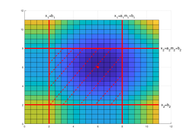
(b) The optimal point (depicted by red circle) in the restricted feasibility region.

Figure 2: Two-dimensional case example.

Motivated by this example, we consider the following convex quadratic problem by taking $\mu_{i}=\nu_{i}=0$ for all $i\in N$:

$$\underset{x,y}{\mathrm{min}}\quad \phi(x,y)=\sum_{i\in N}{x}_{i}{y}_{i}+p(f-\sum_{i\in N}{y}_{i})$$ (8a)

$$\mathrm{subject\ to}\quad \underaccent{\bar}{\rho}\leq{x}_{i}\leq\bar{\rho},\qquad\forall i\in N$$ (8b)

$$\sum_{i\in N}{y}_{i}\leq f,$$ (8c)

$${y}_{i}=\frac{{x}_{i}-b_{i}}{a_{i}},\quad b_{i}\leq{x}_{i}\leq a_{i}m_{i}+b_{i},\quad\forall i\in N.$$ (8d)

It appears that a global minimum of the nonconvex problem (7) can be found by solving the convex problem (8).

Lemma 5.

Assume $\underaccent{\bar}{\rho}-a_{i}m_{i}\leq b_{i}\leq\bar{\rho}$ for all $i\in N$. Then, there exists an optimal solution $x^{*},y^{*},\mu^{*}$ and $\nu^{*}$ for (7) such that $\mu^{*}=\nu^{*}=0$ and the same $x^{*}$ and $y^{*}$ are also the minimizers of the convex quadratic problem (8).

Proof.

See A. ∎

Remark 6.

The piece-wise linear constraint (7d) makes the problem (7) a piece-wise quadratic optimization problem with $3^{n}$ quadratic problems where $n$ is the number of prosumers. Lemma 5 proves that under the assumption $\underaccent{\bar}{\rho}-a_{i}m_{i}\leq b_{i}\leq\bar{\rho}$ for all $i\in N$, one of these $3^{n}$ problems always attains the global optimum.

Now, we are in a position to state the main results of this paper.

Theorem 7.

Consider the optimization problem (7). Let $\alpha=\{i\in N\mid b_{i}>\bar{\rho}\}$, $\beta=\{i\in N\mid a_{i}m_{i}+b_{i}<\underaccent{\bar}{\rho}\}$ and $\theta=\{i\in N\mid\underaccent{\bar}{\rho}-a_{i}m_{i}\leq b_{i}\leq\bar{\rho}\}$. Then,

$$x_{i}^{*}\in[\underaccent{\bar}{\rho},\bar{\rho}],\ y_{i}^{*}=0,\quad\forall\ i\in\alpha,$$ (9)

$$x_{i}^{*}=\underaccent{\bar}{\rho},\ y_{i}^{*}=m_{i},\quad\forall\ i\in\beta,$$ (10)

and $x_{i}^{*},y_{i}^{*}$ for all $i\in\theta$ are the minimizers of the following convex problem:

$$\min_{\begin{subarray}{c}x_{i},y_{i}\\ \forall\ i\in\theta\end{subarray}}\quad \phi(x,y)=\sum_{i\in\theta}{x}_{i}{y}_{i}+\sum_{i\in\beta}\underaccent{\bar}{\rho}m_{i}+p(f-\sum_{i\in\theta}{y}_{i}-\sum_{i\in\beta}{m}_{i})$$ (11a)

$$\mathrm{subject\ to}\quad \underaccent{\bar}{\rho}\leq{x}_{i}\leq\bar{\rho},\qquad\forall i\in\theta,$$ (11b)

$$\sum_{i\in\theta}{y}_{i}\leq f-\sum_{i\in\beta}{m}_{i},$$ (11c)

$${y}_{i}=\frac{{x}_{i}-b_{i}}{a_{i}},\quad b_{i}\leq{x}_{i}\leq a_{i}m_{i}+b_{i},\quad\forall i\in\theta.$$ (11d)

Proof.

The proof for the optimal solutions of the subsets $\alpha$ and $\beta$ immediately follows from Lemma 3. Eliminating this trivial solutions, the proof for the minimizers of indices in $\theta$ follows from Lemma 5. ∎

Another advantage of using the convex optimization problem (11) over the bilevel one stems from privacy considerations. Indeed, the aggregator needs to have all information about the prosumers to the bilevel problem in a centralized way. However, the prosumers may not be willing to share their information with third parties due to privacy concerns. Since Theorem 7 allows a distibuted solution to find the optimum (see [28]), such privacy concerns are not an obstacle for solving the problem (8) or (11).

4 Personalized pricing vs. Uniform pricing

In the setup we have considered so far in this work, a personalized pricing scheme is implemented. This means that the aggregator proposes different prices to each prosumer to minimize its cost. However, in another scenario, one can consider a uniform pricing scheme where the aggregator proposes the same price to all the prosumers [9]. These two pricing schemes are very well-known in microeconomics literrature [29]. In what follows, we investigate the advantages of personalized pricing over uniform pricing in the defined balancing market. For this purpose, we first (re)write the problems for these schemes. The optimization problem PP corresponds to the personalized pricing scheme:

$$\mathrm{PP:}\qquad \underset{x,y,\mu,\nu}{\mathrm{min}}\quad \ \phi(x,y)=\sum_{i\in N}(x_{i}-p)y_{i}+pf$$ (12a)

$$\mathrm{subject\ to}\quad 0\leq x\leq\bar{\rho}\qquad\forall i\in N,$$ (12b)

$$\sum_{i\in N}y_{i}\leq f,$$ (12c)

$$y_{i}=\frac{x_{i}-b_{i}+\mu_{i}-\nu_{i}}{a_{i}},\qquad\forall i\in N,$$ (12d)

$$0\leq y_{i}\perp\mu_{i}\geq 0,\qquad\forall i\in N,$$ (12e)

$$0\leq m_{i}-y_{i}\perp\nu_{i}\geq 0,\qquad\forall i\in N.$$ (12f)

Note that this is a reformulation of the problem (7). For simplicity, we consider the parameter $\underaccent{\bar}{\rho}$ equal to zero, although all the following analyses can be verified for arbitrary $\underaccent{\bar}{\rho}$. Similar to the problem above, we define the problem UP for the uniform pricing scheme. Here all the proposed prices to the prosumers are equal and it is denoted by the scalar decision variable $x$:

$$\mathrm{UP:}\qquad \underset{x,y,\mu,\nu}{\mathrm{min}}\quad \ \phi(x,y)=\sum_{i\in N}(x-p)y_{i}+pf$$ (13a)

$$\mathrm{subject\ to}\quad 0\leq x\leq\bar{\rho},$$ (13b)

$$\sum_{i\in N}y_{i}\leq f,$$ (13c)

$$y_{i}=\frac{x-b_{i}+\mu_{i}-\nu_{i}}{a_{i}},\qquad\forall i\in N,$$ (13d)

$$0\leq y_{i}\perp\mu_{i}\geq 0,\qquad\forall i\in N,$$ (13e)

$$0\leq m_{i}-y_{i}\perp\nu_{i}\geq 0,\qquad\forall i\in N.$$ (13f)

One of the main benefits of the personalized pricing scheme is that it leads to a lower or equal balancing cost. The next proposition states this advantage.

Proposition 8.

The aggregator’s optimal cost in the personalized pricing scheme is less than or equal than its optimal cost in the uniform pricing scheme, i.e.,

$$\phi_{\mathrm{PP}}^{*}\leq\phi_{\mathrm{UP}}^{*}.$$

Proof.

One can rewrite the problem (13) by replacing $x$ by $x_{i}$ and add an extra constraint as

$$x_{1}=x_{2}=\dots=x_{n}.$$

Therefore, the feasible set of the problem UP is a subset of the feasible set of the problem PP. This concludes that $\phi_{\mathrm{PP}}^{*}\leq\phi_{\mathrm{UP}}^{*}$. ∎

Having a less balancing cost for the aggregator is not the only superior aspect of the personalized pricing scheme. The next proposition shows that under this pricing scheme more prosumers contribute to the balancing market.

Proposition 9.

Let $n_{\mathrm{PP}}(N)$ and $n_{\mathrm{UP}}(N)$ be the number of prosumers who participate in the personalized and uniform pricing scheme, respectively. Then, $n_{\mathrm{UP}}(N)\leq n_{\mathrm{PP}}(N)$.

To prove the proposition above, we need some auxiliary results. The following lemmas concerning the optimization problems PP and UP play an essential role in the proof of Proposition 9.

Lemma 10.

Consider the optimization problems PP and UP. Then the following two statements hold.

1. Let $b_{i}<0$ for some $i\in N$. Then, the optimal solution $y_{i}^{*}$ is positive for both problems.

2. Let $b_{i}>\bar{\rho}$ for some $i\in N$. Then, the optimal solution $y_{i}^{*}$ is zero for both problems.

Proof.

See A. ∎

Lemma 11.

Consider the optimization problem PP. Suppose that $0\leq b_{i}\leq\bar{\rho}$ for all $i\in N$. If $p>b_{i}$, then $y_{i}^{*}>0$.

Proof.

See A. ∎

Lemma 11 provides a sufficient condition for contribution of each prosumer in the personalized pricing scheme, whereas the next one provides a necessary condition for contribution of each prosumer in the uniform pricing scheme.

Lemma 12.

Consider the optimization problem UP. Suppose that $0\leq b_{i}\leq\bar{\rho}$ for all $i\in N$. Also, suppose the sets $\gamma=\{i\in N\mid y_{i}^{*}>0\}$ and $\bar{\gamma}=\{i\in N\mid y_{i}^{*}=0\}$ are given. Then, $p>b_{i}$ for all $i\in\gamma$.

Proof.

See A. ∎

Remark 13.

Note that in Lemma 12, $(p-b_{i})$ is sign-indefinite for $i\in\bar{\gamma}$. Therefore, we can argue that there exists $\hat{\gamma}$ such that $N\supseteq\hat{\gamma}\supseteq\gamma$ and $p>b_{i}$ for all $i\in\hat{\gamma}$.

Now, we are in a position to prove Proposition 9.

Proof of Proposition 9.

Define the set, $\alpha=\{i\in N\mid b_{i}<0\}$, $\beta=\{i\in N\mid 0\leq b_{i}\leq\bar{\rho}\}$ and $\theta=\{i\in N\mid b_{i}>\bar{\rho}\}$. Due to Lemma 10, $n_{\mathrm{PP}}(\alpha)=n_{\mathrm{UP}}(\alpha)=\lvert\alpha\rvert$ and $n_{\mathrm{PP}}(\theta)=n_{\mathrm{UP}}(\theta)=0$. Now, suppose that $n_{\mathrm{UP}}(\beta)$ is given. Then, based on Lemma 12, $p>b_{i}$ holds for all $i\in\hat{\gamma}$ where $\hat{\gamma}$ is defined in Remark 13. As a result, due to Lemma 11, $n_{\mathrm{PP}}(\beta)\geq n_{\mathrm{UP}}(\beta)$. Consequently, we have $n_{\mathrm{PP}}(N)\geq n_{\mathrm{UP}}(N)$. ∎

The profit of a single prosumer in the personalized pricing scheme might be higher or lower than its profit in the uniform pricing scheme. Nonetheless, Proposition 9 states that the chance of participation of a prosumer and having revenue in the balancing market is higher in the personalized scheme.

5 Simulations

In this section, first we evaluate the performance of our convex equivalent problem for the rtbm in terms of computation time and optimality. We use the state-of-the-art mip-based approach in [27] as a benchmark for this evaluation. Next, we compare the aggregator’s cost and prosumers’ contribution under two schemes: personalized and uniform pricing.

For simulation purposes, we consider one type of hp and two types of mchp technologies for the prosumers. We assume that half of the prosumers have hp and the other half are equipped with mchp. We assign to each prosumer a specific technology of hp or mchp, randomly. Tables 1 and 2 show the data regarding these types and also their corresponding $\lvert b_{i}\rvert$ parameters. The supplier gas and electricity prices are based on data from [30] for the Netherlands and equal to $0.0861\ \text{€}/\mathrm{kWh}$ and $0.1707\ \text{€}/\mathrm{kWh}$, respectively. The price $p$ for both up- and down-regulation is set to $0.7\ \text{€}/\mathrm{kWh}$ based on the settlement price data of TenneT from [31] for a period where the tso is under high stress. It should be noted that the tso informs the aggregators about this price ex-ante. Also, we assume that $\bar{\rho}=p=0.7$ and $\underaccent{\bar}{\rho}=0$.

All optimization problems are implemented in MATLAB r2018b and solved by the Gurobi Optimizer [32]. The simulations were run on four Intel Xeon 2.6 GHz cores and 1024 GB internal memory of the Peregrine high performance computing cluster of the University of Groningen.

Table 1: The parameters for different hp technologies.

hp type	Nominal electricity input power	$\lvert b_{i}\rvert$
$1$	$1.1\ kW$	$0.1707\ \text{€}/kWh$

Table 2: The parameters for different mchp technologies.

mchp type	Nominal input power	Nominal electricity output power	$\lvert b_{i}\rvert$
$1$	$8\ kW$	$1\ kW$	$0.6888\ \text{€}/{kWh}$
$2$	$4.7\ kW$	$0.8\ kW$	$0.5088\ \text{€}/{kWh}$

5.1 Computation time and optimality comparison

Here, we first define the mip formulation of the problem (2). This formulation is used as a benchmark to evaluate the computational efficiency of the convex equivalent of the bilevel problem. By introducing dual variables $\lambda_{1i},\lambda_{2i}$, auxiliary binary variables $z_{i},w_{i}$ and a sufficiently large constant $M$, the problem (2) can be turned to an mip problem as

$$\underset{w,y,z,\lambda_{1},\lambda_{2}}{\mathrm{min}}\quad \sum_{i}(a_{i}y_{i}^{2}+(b_{i}-p)y_{i}+m_{i}\lambda_{2i})+pf$$ (14a)

$$\mathrm{subject\ to}\quad \sum_{i}y_{i}\leq f,$$ (14b)

$$\begin{cases}x_{i}=a_{i}y_{i}+b_{i}-\lambda_{1i}+\lambda_{2i}\geq 0,\\ x_{i}=a_{i}y_{i}+b_{i}-\lambda_{1i}+\lambda_{2i}\leq\bar{\rho},\\ 0\leq y_{i}\leq Mz_{i},\\ 0\leq m_{i}-y_{i}\leq Mw_{i},\\ 0\leq\lambda_{1i}\leq M(1-z_{i}),\\ 0\leq\lambda_{2i}\leq M(1-w_{i}),\end{cases}\quad\forall i\in N.$$ (14c)

Details of this approach can be found in [27].

The mip solvers use complicated heuristic methods to find the optimal solution. Moreover, the computation time for computing an optimal solution is highly related to specific parameters of the problem. To find a rough estimate of the optimization run time, we implement a set of 1000 Monte Carlo simulations with uniformly generated random parameters $a_{i}$, $m_{i}$ and $f$ for the optimization problem. This is done for different numbers of prosumers. Table 3 summarizes the run time results for these Monte Carlo scenarios. The last column of this table shows the number of scenarios (out of 1000 Monte Carlo scenarios) where the mip problem leads to an infeasible solution or an optimal solution with higher cost than the convex problem.

The computation time for the convex optimization problem grows approximately linear with respect to the number of prosumers. This can be seen from the average run time in Table 3 for the convex formulation. If we consider $30000$ as the typical number of prosumers for an aggregator, then the average and the maximum run time are acceptable for a real-time application with $5$-minute time interval. However, this is not the case for an mip formulation. Figure 3 and Table 3 show that the average and maximum computation time of mip is not suitable for a real-time market since the computational time grows approximately exponentially. Moreover, there are some cases that the mip formulation with high number of optimization variables does not converge to the global optimal or even to feasible solution. This is shown on the last column of Table 3. For instance, for $10$-prosumer case, both the mip and convex formulation have the same optimal solution in all $1000$ random scenarios. Nevertheless, in $30000$-prosumer case, the mip formulation converges to a higher minimum cost or an infeasible solution with respect to the convex formulation in $40$ out of $1000$ random scenarios of the simulations. It is clear that in the rest $960$ scenarios both the formulations have the same optimal solution.

Table 3: Simulation run time and optimality comparison.

Number of Prosumers	Convex formulation run time		mip formulation run time		Number of scenarios with infeasible
	Average (sec)	Maximum (sec)	Average (sec)	Maximum (sec)	or non-optimal solution for mip
10	0.0006	0.0010	0.0016	0.0039	0
100	0.0012	0.0017	0.0032	0.0058	0
1000	0.0038	0.0076	0.0128	0.0371	1
10000	0.0344	0.0484	0.5548	9.0352	11
20000	0.0772	0.1231	3.9498	59.1761	27
30000	0.1161	0.1834	11.1190	161.7937	40

Figure 3: Maximum run time: Convex vs. mip formulation.

5.2 Pricing schemes comparison

Table 4: The prosumers’ parameters for pricing scheme comparison.

Pro. number	mchp type	$a_{i}\ (\text{€}/kWh^{2})$	$b_{i}\ (\text{€}/{kWh})$	$m_{i}\ (kWh)$
$1$	Type $1$	$2$	$0.6888$	$0.08$
$2$	Type $1$	$5$	$0.6888$	$0.05$
$3$	Type $2$	$10$	$0.5088$	$0.02$
$4$	Type $2$	$5$	$0.5088$	$0.01$
$5$	Type $2$	$20$	$0.5088$	$0.025$

This subsection is devoted to show the validity of Proposition 8 and 9. We consider a case where the aggregator and TSO are in down regulation. The total number of prosumers is assumed to be $5$ and all are equipped with mchps. The full details of prosumers’ parameters are presented in Table 4. The requested flexibility $f$ is $0.05\ \mathrm{kWh}$. The results for both pricing schemes are demonstrated in Table 5.

The optimal results in Table 5 shows that all prosumers contribute to the balancing market under the personalized pricing scheme. However, in the uniform pricing scheme, only the prosumer number $3$, $4$ and $5$ provide flexibility. Furthermore, the aggregator’s optimal cost in the personalized pricing scheme is less than its optimal cost in the uniform pricing scheme. Indeed, this is inline with what is claimed in Section 4.

Table 5: Optimal price and flexibility: Personalized pricing vs. Uniform pricing

Prosumer number	Personalized pricing scheme		Uniform pricing scheme
	$x_{i}^{*}\ (\text{€}/kWh)$	$y_{i}^{*}\ (kWh)$	$x_{i}^{*}\ (\text{€}/kWh)$	$y_{i}^{*}\ (kWh)$
$1$	$0.6944$	$0.0028$	$0.5711$	$0$
$2$	$0.6944$	$0.0011$	$0.5711$	$0$
$3$	$0.6044$	$0.0096$	$0.5711$	$0.0062$
$4$	$0.5588$	$0.0010$	$0.5711$	$0.0100$
$5$	$0.6044$	$0.0048$	$0.5711$	$0.0031$
Agg. cost (€)	$0.0322$		$0.0335$

6 Conclusions

In this paper, we have developed a market with a tso, an aggregator and prosumers to address real-time balancing. We have modeled the corresponding economic optimization problem of a self-interested aggregator and prosumers as a bilevel optimization problem under a personalized pricing scheme. Generally, bilevel optimization problems are non-convex. We have shown that it suffices to solve a specific convex optimization problem to find the global optimum of the original bilevel optimization problem. In contrast to existing approaches (e.g., mip), the convex equivalent of the bilevel optimization problem has very low computation time and is therefore preferable in real-time. Low computation time and global optimality are not the only advantages of having a convex equivalent for the bilevel optimization. Centralized aggregator control over the whole community of prosumers can be a difficult task, especially when the number of prosumers is very high. However, having a convex formulation for the balancing problem opens up new horizons in decentralized and distributed control and optimization.

Also, we have compared the optimal solutions for two pricing scheme, i.e., personalized and uniform pricing scheme. We have shown, in a rigorous mathematical way, that under the personalized pricing scheme more prosumers contribute to the balancing market and the aggregator’s optimal cost is less.

Appendix A Proofs of lemmas

Proof of Lemma 1.

The proof is evident from the fact that the optimization problem (2e) is a convex optimization problem in $y_{i1}$ and $y_{i2}$ for any given $x_{i}$ and the KKT conditions are necessary and sufficient for this problem. ∎

Proof of Lemma 2.

Let $x_{i}^{*},y_{i1}^{*},y_{i2}^{*},\mu_{i1}^{*},\mu_{i2}^{*},\nu_{i1}^{*}$ and $\nu_{i2}^{*}$ be the optimal solution of the problem (4).

1. Suppose, on the contrary, that $y_{i1}^{*}y_{i2}^{*}\neq 0$. Therefore, $\mu_{i1}^{*}=\mu_{i2}^{*}=0$ and we have

   $$a_{i1}y_{i1}^{*}-\sqrt{a_{i1}a_{i2}}y^{*}_{i2}+b_{i1}-x_{i}^{*}+\nu_{i1}^{*}=0,$$ (15)

   $$-\sqrt{a_{i1}a_{i2}}y_{i1}^{*}+a_{i2}y_{i2}^{*}+b_{i2}-x_{i}^{*}+\nu_{i2}^{*}=0.$$ (16)

   We multiply (15) by $\sqrt{a_{i2}}$ and (16) by $\sqrt{a_{i1}}$. By adding these two terms, we get

   $$x_{i}^{*}\geq\frac{\sqrt{a_{i2}}b_{i1}+\sqrt{a_{i1}}b_{i2}}{\sqrt{a_{i1}}+\sqrt{a_{i2}}},$$

   which is a contradiction since $x_{i}^{*}\leq\bar{\rho}$. Therefore, either $y_{i1}^{*}$ or $y_{i2}^{*}$ is zero.

2. Since $b_{i2}\geq b_{i1}$, we have $b_{i2}\geq\frac{\sqrt{a_{i2}}b_{i1}+\sqrt{a_{i1}}b_{i2}}{\sqrt{a_{i1}}+\sqrt{a_{i2}}}>\bar{\rho}$. Suppose, on the contrary, that $y_{i2}^{*}>0$. Then, based on item I, $y_{i1}^{*}=0$. This point should satisfy the constraints of (4), specifically,

   $$a_{i2}y_{i2}^{*}+b_{i2}-x_{i}^{*}+\nu_{i2}^{*}=0,\qquad x_{i}^{*}\leq\bar{\rho}.$$

   The first equality yields to $x^{*}_{i}>b_{i2}$ which contradicts $x_{i}^{*}\leq\bar{\rho}$, since $b_{i2}>\bar{\rho}$. Therefore, $y_{i2}^{*}=0$.

3. The proof is similar to that of the previous statement.

∎

Proof of Lemma 3.

1. Since $b_{i}>\bar{\rho}$, for any feasible $x_{i}$ such that $\bar{\rho}\geq x_{i}\geq\underaccent{\bar}{\rho}$, we can write $b_{i}>\bar{\rho}\geq{x_{i}}\geq\underaccent{\bar}{\rho}$. Therefore, $x_{i}<b_{i}$. Then, based on the objective function (7a) and the constraint (7d) , we can conclude that $x_{i}^{*}\in[\underaccent{\bar}{\rho},\bar{\rho}]$, $y_{i}^{*}=0$, $\mu_{i}^{*}=b_{i}-x_{i}^{*}$ and $\nu_{i}^{*}=0$.

2. Since $\underaccent{\bar}{\rho}>a_{i}m_{i}+b_{i}$, for any feasible $x_{i}$ such that $\bar{\rho}\geq x_{i}\geq\underaccent{\bar}{\rho}$, we can write $\bar{\rho}\geq{x_{i}}\geq\underaccent{\bar}{\rho}>a_{i}m_{i}+b_{i}$. Therefore, $x_{i}>a_{i}m_{i}+b_{i}$. Then, based on (7d), we can conclude that $x_{i}^{*}=\underaccent{\bar}{\rho}$, $y_{i}^{*}=m_{i}$, $\mu_{i}^{*}=0$ and $\nu_{i}^{*}=x_{i}^{*}-a_{i}m_{i}-b_{i}$.

∎

Proof of Lemma 5.

We consider two cases. Note that since $m_{i}>0$, $\mu_{i}$ and $\nu_{i}$ cannot be nonzero at the same time.

Case 1)

Suppose, for the sake of contradiction, $x_{i}^{*}$, $y_{i}^{*}$, $\mu_{i}^{*}$ and $\nu_{i}^{*}$ be the only optimal solution of the problem (7) and $\mu_{i}^{*}>0$ and $\nu_{i}^{*}=0$. Since $x_{i}^{*}$, $y_{i}^{*}$, $\mu_{i}^{*}$ and $\nu_{i}^{*}$ are an optimal solution and hence are feasible, they should satisfy the constraints of the problem (7), .i.e.

$$\underaccent{\bar}{\rho}\leq x_{i}^{*}\leq\bar{\rho},$$

$$y_{i}^{*}+\sum_{j\in N\atop j\neq i}y_{j}^{*}\leq f,$$

$$y_{i}^{*}=0,\ \mu_{i}^{*}=b_{i}-x_{i}^{*},\ \nu_{i}^{*}=0$$

We define $\bar{x}_{i}=x_{i}^{*}+\mu_{i}^{*}=b_{i}$ and consequently we have

$$\bar{y_{i}}=0,\ \bar{\mu}_{i}=0,\ \bar{\nu}_{i}=0.$$

Since $b_{i}\leq\bar{\rho}$, $\bar{x}_{i}>x_{i}^{*}$ and $\bar{y}_{i}=y_{i}^{*}=0$, we can conclude that $\bar{x}_{i}$, $\bar{y}_{i}$, $\bar{\mu}_{i}$ and $\bar{\nu}_{i}$ are feasible for (7) and $\phi(x_{i}^{*},y_{i}^{*})=\phi(\bar{x}_{i},\bar{y}_{i})$ which is a contradiction.

Case 2)

Suppose, for the sake of contradiction, $x_{i}^{*}$, $y_{i}^{*}$, $\mu_{i}^{*}$ and $\nu_{i}^{*}$ be an optimal solution of the problem (7) and $\mu_{i}^{*}=0$ and $\nu_{i}^{*}>0$. Since $x_{i}^{*}$, $y_{i}^{*}$, $\mu_{i}^{*}$ and $\nu_{i}^{*}$ are an optimal solution and hence are feasible, they should satisfy the constraints of the problem (7), .i.e.,

$$\underaccent{\bar}{\rho}\leq x_{i}^{*}\leq\bar{\rho},$$

$$y_{i}^{*}+\sum_{j\in N\atop j\neq i}y_{j}^{*}\leq f,$$

$$y_{i}^{*}=m_{i},\ \mu_{i}^{*}=0,\ \nu_{i}^{*}=x_{i}^{*}-a_{i}m_{i}-b_{i}.$$

We define $\bar{x}_{i}=x_{i}^{*}-\nu_{i}^{*}=a_{i}m_{i}+b_{i}$ and consequently we have

$$\bar{y_{i}}=m_{i},\ \bar{\mu}_{i}=0,\ \bar{\nu}_{i}=0.$$

Since $a_{i}m_{i}+b_{i}\geq\underaccent{\bar}{\rho}$, $\bar{x}_{i}<x_{i}^{*}$ and $\bar{y}_{i}=y_{i}^{*}=m_{i}>0$, we can conclude that $\bar{x}_{i}$, $\bar{y}_{i}$, $\bar{\mu}_{i}$ and $\bar{\nu}_{i}$ are feasible for (7) and $\phi(\bar{x}_{i},\bar{y}_{i})<\phi(x_{i}^{*},y_{i}^{*})$ which is a contradiction.

By means of these two cases, we show that there exists an optimal solution $x_{i}^{*}$, $y_{i}^{*}$, $\mu_{i}^{*}=0$ and $\nu_{i}^{*}=0$ for all $i\in N$ for the problem (7). As a result, we can relax $\mu_{i}$ and $\nu_{i}$ to zero in (7) for all $i\in N$ and thus the same $x_{i}^{*}$ and $y_{i}^{*}$ can be found as the solution of (8). ∎

Proof of Lemma 10.

1. Problem PP: Let $x_{i},y_{i},\mu_{i}$ and $\nu_{i}$ be any feasible solution for (12). Since $x_{i}$ is nonnegative and $b_{i}$ is negative, we have $x_{i}-b_{i}>0$ and $\mu_{i}=0$. If $\nu_{i}=0$, then $y_{i}=\frac{x_{i}-b_{i}}{a_{i}}>0$ and if $\nu_{i}>0$, then $y_{i}=m_{i}>0$. Therefore, $y_{i}$ is positive if $b_{i}$ is negative.
   Problem UP: The proof is similar to the previous case.

2. Problem PP: It follows from Lemma 3 item I.
   Problem UP: The proof is similar to the proof of Lemma 3 item I.

∎

Proof of Lemma 11.

Since $0\leq b_{i}\leq\bar{\rho}$ for all $i\in N$, based on Lemma 5, $\mu_{i}^{*}=\nu_{i}^{*}=0$ for all $i\in N$ in (12). Suppose, for the sake of contradiction, there exists $j\in N$ such that $y_{j}^{*}=0$ and $x_{j}^{*}=b_{j}$. We can leave out the constraints corresponding to the index $j$ from the problem (12). As a result, the following optimization problem has the same optimizer:

$$\underset{x,y}{\mathrm{min}}\quad \ (x_{j}-p)(\frac{x_{j}-b_{j}}{a_{j}})+\sum_{i\in N\atop i\neq j}(x_{i}-p)(\frac{x_{i}-b_{i}}{a_{i}})+pf$$ (17a)

$$\mathrm{subject\ to}\quad 0\leq x_{i}\leq\bar{\rho},\qquad\forall i\in N\setminus\{j\},$$ (17b)

$$\frac{x_{i}-b_{i}}{a_{i}}\geq 0,\qquad\forall i\in N\setminus\{j\},$$ (17c)

$$\frac{x_{i}-b_{i}}{a_{i}}\leq m_{i}\qquad\forall i\in N\setminus\{j\},$$ (17d)

$$\sum_{i\in N\atop i\neq j}\frac{x_{i}-b_{i}}{a_{i}}\leq f,$$ (17e)

where $\frac{x_{i}-b_{i}}{a_{i}}=y_{i}$. This optimization problem is convex. Therefore, the optimizer of this problem satisfies the KKT conditions. We write the KKT conditions of this problem for the index $j$ as follows:

$$x_{j}^{*}=\frac{b_{j}+p}{2}.$$

Having $x_{j}^{*}=b_{j}$, we conclude $b_{j}=p$ which is a contradiction since $b_{i}<p$ for all $i\in N$. ∎

Proof of Lemma 12.

We define index sets $\gamma_{1}=\{i\in\gamma\mid\nu_{i}^{*}=0\}$ and $\gamma_{2}=\{i\in\gamma\mid\nu_{i}^{*}>0\}$. Based on the sets $\gamma_{1}$, $\gamma_{2}$, $\bar{\gamma}$ and the complementary constraints of the problem (13), the following can be concluded.

$$y_{i}^{*}>0,\quad \mu_{i}^{*}=0,\quad \nu_{i}^{*}=0, \forall\ i\in\gamma_{1},$$

$$y_{i}^{*}=m_{i},\quad \mu_{i}^{*}=0,\quad \nu_{i}^{*}>0, \forall\ i\in\gamma_{2},$$

$$y_{i}^{*}=0,\quad \mu_{i}^{*}\geq 0,\quad \nu_{i}^{*}=0, \forall\ i\in\bar{\gamma}$$

As a result, the next optimization problem has the same optimizer as (13).

$$\underset{x,y,\mu.\nu}{\mathrm{min}}\quad \ (x-p)(\sum_{i\in\gamma_{1}}y_{i}+\sum_{i\in\gamma_{2}}m_{i})+pf$$ (18a)

$$\mathrm{subject\ to}\quad y_{i}=\frac{x-b_{i}}{a_{i}}\geq 0\qquad\forall i\in\gamma_{1},$$ (18b)

$$\nu_{i}=x-a_{i}m_{i}-b_{i}\geq 0,\qquad\forall i\in\gamma_{2},$$ (18c)

$$\mu_{i}=b_{i}-x\geq 0,\qquad\forall i\in\bar{\gamma},$$ (18d)

$$\sum_{i\in\gamma_{1}}y_{i}\leq f-\sum_{i\in\gamma_{2}}m_{i}$$ (18e)

Let $\lambda_{1i}$, $\lambda_{2i}$, $\lambda_{3i}$ and $\lambda_{4}$ be the dual variables for the constraints (18b)-(18e), respectively. Since this problem is convex, the KKT conditions are necessary and sufficient for the optimizer of this problem. Note that since $y_{i}^{*}>0$, $\lambda_{1i}^{*}=0$ for all $i\in\gamma_{1}$ and since $v_{i}^{*}>0$, $\lambda_{2i}^{*}=0$ for all $i\in\gamma_{2}$.

$$x^{*}=\frac{p}{2}+\frac{\chi}{2}-\omega$$ (19)

$$x^{*}>b_{i},\qquad\forall i\in\gamma_{1},$$ (20)

$$x^{*}>a_{i}m_{i}+b_{i},\qquad\forall i\in\gamma_{2},$$ (21)

$$b_{i}\geq x_{i}\perp\lambda_{3i}^{*}\geq 0,\qquad\forall i\in\bar{\gamma},$$ (22)

$$f-\sum_{i\in\gamma_{2}}m_{i}\geq\sum_{i\in\gamma_{1}}\frac{x-b_{i}}{a_{i}}\perp\lambda_{4}^{*}\geq 0$$ (23)

where

$$\chi=\frac{\displaystyle\sum_{i_{1}\in\gamma_{1}}(b_{i_{1}}\prod_{{i_{2}}\in\gamma_{1}\atop i_{2}\neq i_{1}}a_{i_{2}})}{\displaystyle\sum_{i_{1}\in\gamma_{1}}\prod_{i_{2}\in\gamma_{1}\atop i_{2}\neq i_{1}}a_{i_{2}}},$$

$$\omega=\frac{\displaystyle\prod_{i_{1}\in\gamma_{1}}a_{i_{1}}}{\displaystyle 2\sum_{i_{1}\in\gamma_{1}}\prod_{i_{2}\in\gamma_{1}\atop i_{2}\neq i_{1}}a_{i_{2}}}(\sum_{i_{1}\in\gamma_{2}}m_{i_{1}}+\sum_{i_{1}\in\bar{\gamma}}\lambda_{3{i_{1}}}+\lambda_{4}\sum_{i_{1}\in\gamma_{1}}\frac{1}{a_{i_{1}}}).$$

Then, we have the following results.

• Let $j\in\gamma_{1}$ and $k\in\gamma_{1}\setminus\{j\}$. Since $\omega$ is positive, we can conclude from (19) and (20)

  $$x^{*}=\frac{p}{2}+\frac{\chi}{2}-\omega>b_{j}\quad\Longrightarrow\quad p>2b_{j}-\chi,$$

  $$x^{*}=\frac{p}{2}+\frac{\chi}{2}-\omega>b_{k}\quad\Longrightarrow\quad p>2b_{k}-\chi.$$

  We multiply $p>2b_{j}-\chi$ by

  $$\sum_{i_{1}\in\gamma_{1}}(\prod_{i_{2}\in\gamma_{1}\atop i_{2}\neq i_{1}}a_{i_{2}})+\prod_{i_{2}\in\gamma_{1}\atop i_{2}\neq j}a_{i_{2}},$$

  and we multiply $p>2b_{k}-\chi$ for all $k\in\gamma_{1}\setminus\{j\}$ by

  $$\prod_{i_{2}\in\gamma_{1}\atop i_{2}\neq k}a_{i_{2}}.$$

  By adding these inequalities together, we have $p>b_{j}$.

• Let $j\in\gamma_{2}$. Due to (19) and (21), we have

  $$x^{*}=\frac{p}{2}+\frac{\chi}{2}-\omega>a_{j}m_{j}+b_{j}>b_{j}\quad\Longrightarrow\quad\chi+p>2b_{j}.$$

  Since $\chi$ is a weighted average of the elements of the set $\{b_{i}\mid i\in\gamma_{1}\}$, there exists $k\in\gamma_{1}$ such that $b_{k}\geq\chi$. Also, since $k\in\gamma_{1}$, we have $p>b_{k}$. Therefore,

  $$\begin{cases}\chi+p>2b_{j},\\ b_{k}\geq\chi,\\ p>b_{k},\end{cases}\quad\Longrightarrow\quad p>b_{j}.$$

∎

References

- [1] Y. Parag, B. K. Sovacool, Electricity market design for the prosumer era, Nature Energy 1 (4) (2016) 1–6. doi:http://doi.org/10.1038/nenergy.2016.32.
- [2] S. Pineda, A. J. Conejo, Using electricity options to hedge against financial risks of power producers, Journal of Modern Power Systems and Clean Energy 1 (2) (2013) 101–109. doi:https://doi.org/10.1007/s40565-013-0018-y.
- [3] Q. Wang, C. Zhang, Y. Ding, G. Xydis, J. Wang, J. Østergaard, Review of real-time electricity markets for integrating distributed energy resources and demand response, Applied Energy 138 (2015) 695–706. doi:https://doi.org/10.1016/j.apenergy.2014.10.048.
- [4] A. J. Conejo, J. M. Morales, L. Baringo, Real-time demand response model, IEEE Transactions on Smart Grid 1 (3) (2010) 236–242. doi:https://doi.org/10.1109/TSG.2010.2078843.
- [5] L. Gkatzikis, I. Koutsopoulos, T. Salonidis, The role of aggregators in smart grid demand response markets, IEEE Journal on Selected Areas in Communications 31 (7) (2013) 1247–1257. doi:https://doi.org/10.1109/JSAC.2013.130708.
- [6] J. S. Vardakas, N. Zorba, C. V. Verikoukis, A survey on demand response programs in smart grids: Pricing methods and optimization algorithms, IEEE Communications Surveys & Tutorials 17 (1) (2014) 152–178. doi:https://doi.org/10.1109/COMST.2014.2341586.
- [7] B. Colson, P. Marcotte, G. Savard, An overview of bilevel optimization, Annals of Operations Research 153 (1) (2007) 235–256. doi:https://doi.org/10.1007/s10479-007-0176-2.
- [8] H. Von Stackelberg, Market Structure and Equilibrium, Springer Science & Business Media, 2010. doi:https://doi.org/10.1007/978-3-642-12586-7.
- [9] M. Zugno, J. M. Morales, P. Pinson, H. Madsen, A bilevel model for electricity retailers’ participation in a demand response market environment, Energy Economics 36 (2013) 182–197. doi:https://doi.org/10.1016/j.eneco.2012.12.010.
- [10] F.-L. Meng, X.-J. Zeng, A bilevel optimization approach to demand response management for the smart grid, in: 2016 IEEE Congress on Evolutionary Computation (CEC), IEEE, 2016, pp. 287–294. doi:https://doi.org/10.1109/CEC.2016.7743807.
- [11] W. Tushar, C. Yuen, D. B. Smith, H. V. Poor, Price discrimination for energy trading in smart grid: A game theoretic approach, IEEE Transactions on Smart Grid 8 (4) (2016) 1790–1801. doi:https://doi.org/10.1109/TSG.2015.2508443.
- [12] J. Yang, J. Zhao, F. Wen, Z. Dong, A model of customizing electricity retail prices based on load profile clustering analysis, IEEE Transactions on Smart Grid 10 (3) (2018) 3374–3386. doi:https://doi.org/10.1109/TSG.2018.2825335.
- [13] J. Yang, J. Zhao, F. Wen, Z. Y. Dong, A framework of customizing electricity retail prices, IEEE Transactions on Power Systems 33 (3) (2017) 2415–2428. doi:https://doi.org/10.1109/TPWRS.2017.2751043.
- [14] W. Tushar, W. Saad, H. V. Poor, D. B. Smith, Economics of electric vehicle charging: A game theoretic approach, IEEE Transactions on Smart Grid 3 (4) (2012) 1767–1778. doi:https://doi.org/10.1109/TSG.2012.2211901.
- [15] B. F. Hobbs, C. B. Metzler, J. S. Pang, Strategic gaming analysis for electric power systems: An MPEC approach, IEEE Transactions on Power Systems 15 (2) (2000) 638–645. doi:https://doi.org/10.1109/59.867153.
- [16] W. Tushar, J. A. Zhang, D. B. Smith, H. V. Poor, S. Thiébaux, Prioritizing consumers in smart grid: A game theoretic approach, IEEE Transactions on Smart Grid 5 (3) (2014) 1429–1438. doi:https://doi.org/10.1109/TSG.2013.2293755.
- [17] R. Li, W. Wei, S. Mei, Q. Hu, Q. Wu, Participation of an energy hub in electricity and heat distribution markets: An MPEC approach, IEEE Transactions on Smart Grid (2018). doi:https://doi.org/10.1109/TSG.2018.2833279.
- [18] C. Wang, W. Wei, J. Wang, F. Liu, S. Mei, Strategic offering and equilibrium in coupled gas and electricity markets, IEEE Transactions on Power Systems 33 (1) (2017) 290–306. doi:https://doi.org/10.1109/TPWRS.2017.2698454.
- [19] A. G. Vlachos, P. N. Biskas, Demand response in a real-time balancing market clearing with pay-as-bid pricing, IEEE Transactions on Smart Grid 4 (4) (2013) 1966–1975. doi:https://doi.org/10.1109/TSG.2013.2256805.
- [20] M. Ghamkhari, A. Sadeghi-Mobarakeh, H. Mohsenian-Rad, Strategic bidding for producers in nodal electricity markets: A convex relaxation approach, IEEE Transactions on Power Systems 32 (3) (2016) 2324–2336. doi:https://doi.org/10.1109/TPWRS.2016.2595593.
- [21] Z. Q. Luo, J. S. Pang, D. Ralph, Mathematical Programs with Equilibrium Constraints, Cambridge University Press, 1996. doi:https://doi.org/10.1017/CBO9780511983658.
- [22] K. Shomalzadeh, J. M. Scherpen, M. K. Camlibel, On the solution of a bilevel electricity market optimization problem, in: 2020 European Control Conference (ECC), IEEE, 2020, pp. 1354–1357, extended abstract. doi:https://doi.org/10.23919/ECC51009.2020.9143634.
- [23] Y. Ding, S. Pineda, P. Nyeng, J. Østergaard, E. M. Larsen, Q. Wu, Real-time market concept architecture for EcoGrid EU—A prototype for European smart grids, IEEE Transactions on Smart Grid 4 (4) (2013) 2006–2016. doi:https://doi.org/10.1109/TSG.2013.2258048.
- [24] J. Yang, J. Zhao, F. Luo, F. Wen, Z. Y. Dong, Decision-making for electricity retailers: A brief survey, IEEE Transactions on Smart Grid 9 (5) (2017) 4140–4153. doi:https://doi.org/10.1109/TSG.2017.2651499.
- [25] R. Deng, Z. Yang, J. Chen, N. R. Asr, M.-Y. Chow, Residential energy consumption scheduling: A coupled-constraint game approach, IEEE Transactions on Smart Grid 5 (3) (2014) 1340–1350. doi:https://doi.org/10.1109/TSG.2013.2287494.
- [26] P. Hansen, B. Jaumard, G. Savard, New branch-and-bound rules for linear bilevel programming, SIAM Journal on Scientific and Statistical Computing 13 (5) (1992) 1194–1217. doi:https://doi.org/10.1137/0913069.
- [27] J. Fortuny-Amat, B. McCarl, A representation and economic interpretation of a two-level programming problem, Journal of the Operational Research Society 32 (9) (1981) 783–792. doi:https://doi.org/10.2307/2581394.
- [28] D. Bertsekas, Nonlinear Programming, Athena Scientific, 1999.
- [29] R. L. Phillips, Pricing and revenue optimization, Stanford university press, 2021. doi:https://doi.org/10.1515/9781503614260.
- [30] Eurosata, Electricity price statistics, retrieved from https://ec.europa.eu/eurostat/statistics-explained/index.php/Electricity_price_statistics. Accessed December 2019 (2019).
- [31] Tennet, Tennet settlement prices, retrieved from https://www.tennet.org/english/operational_management/System_data_relating_processing/settlement_prices/index.aspx. Accessed December 2019 (2019).
- [32] Guobi, Gurobi optimizer reference manual, http://www.gurobi.com (2019).