Continuous Time Random Walk in a velocity field: Role of domain growth, Galilei-invariant advection-diffusion, and kinetics of particle mixing

Abstract

We consider the emerging dynamics of a separable Continuous Time Random Walk (CTRW) in the case when the random walker is biased by a velocity field in a uniformly growing domain. Concrete examples for such domains include growing biological cells or lipid vesicles, biofilms and tissues, but also macroscopic systems such as expanding aquifers during rainy periods, or the expanding universe. The CTRW in this study can be subdiffusive, normal diffusive or superdiffusive, including the particular case of a Lévy flight. We first consider the case when the velocity field is absent. In the subdiffusive case, we reveal an interesting time dependence of the kurtosis of the particle probability density function. In particular, for a suitable parameter choice, we find that the propagator, which is fat tailed at short times, may cross over to a Gaussian-like propagator. We subsequently incorporate the effect of the velocity field and derive a bi-fractional diffusion-advection equation encoding the time evolution of the particle distribution. We apply this equation to study the mixing kinetics of two diffusing pulses, whose peaks move towards each other under the action of velocity fields acting in opposite directions. This deterministic motion of the peaks, together with the diffusive spreading of each pulse, tends to increase particle mixing, thereby counteracting the peak separation induced by the domain growth. As a result of this competition, different regimes of mixing arise. In the case of Lévy flights, apart from the non-mixing regime, one has two different mixing regimes in the long-time limit, depending on the exact parameter choice: In one of these regimes, mixing is mainly driven by diffusive spreading, while in the other mixing is controlled by the velocity fields acting on each pulse. Possible implications for encounter-controlled reactions in real systems are discussed.

1 Introduction

Since its introduction by Montroll and Weiss in the mid 60s [1], the celebrated Continuous Time Random Walk (CTRW) model has found widespread application in statistical physics and beyond, notably in the study of problems as diverse as charge carrier transport in disordered media such as amorphous semiconductors [2, 3, 4], luminescence quenching [5], morphogen gradient formation [6, 7], the diffusive motion of water molecules in the hydration shell around proteins [8], the relative motion of monomers in a protein molecule [9], the motion of protein channels in the cell membrane [10] of lipid and insulin granules [11, 12], or of active transport [13, 14] in living biological cells, up to chemical tracer dispersion in groundwater aquifers [15, 16], and even ageing effects in stock markets [17, 18]. Several review articles and monographs have devoted substantial parts on CTRW [19, 20, 21, 22, 23, 24, 25, 26, 27, 28, 29]. Specific properties of the CTRW concern the concept of weak ergodicity breaking [30, 32, 31, 33, 34] and ageing [35, 36, 37, 38, 39].

In the original version of the CTRW model, the probability density functions (PDFs) of the waiting times (also called trapping or sojourn times) between successive jumps and of the lengths of individual jumps are assumed to decouple, that is, are independent of each other. In the case when the PDF of the waiting times $\tau$ is fat-tailed and scale-free, $\psi(\tau)\simeq\tau^{-1-\alpha}$ with $0<\alpha<1$, and the variance of the jump length PDF is finite, the long-time limit of the model is known to yield anomalous diffusion in the subdiffusive range with the mean-squared displacement $\langle x^{2}(t)\rangle\simeq t^{\alpha}$ [1, 2, 3, 22, 23, 24, 25, 26]. In the more general case, given specific forms of the waiting time and jump length PDFs, the emerging behaviour may be subdiffusive, diffusive, or superdiffusive. This versatility of the model, together with the fact that it can be shown to be equivalent to a generalised master equation [40] and a fractional diffusion equation (FDE) in the anomalous diffusion case [41, 42, 43] makes the CTRW a popular choice to model anomalous transport. One of the advantages of the FDE formulation is that it can incorporate the effect of external force fields and various boundary conditions in a natural and transparent way [23, 24, 44]. Further generalisations are also possible, for instance, accounting for the effect of finite lifetimes of tracer particles (so called “evanescent” or “mortal walkers”) [45, 7, 46, 47], or of chemical reactions occurring at random times and locations [48, 49, 53, 50, 51, 52, 54, 55, 57, 56, 58].

Recently, it has been discussed how separable CTRWs need to be formulated when the domain, on which the process is running off, is itself explicitly evolving in time. In particular, it has been shown that an FDE can be derived [59, 60, 61, 62], whence the case of normal diffusion on an evolving domain [63] is recovered in the appropriate limit. The obtained FDE applies when the diffusing particles stick to the evolving domain, implying that they experience a drift even when they do not jump. The interplay between diffusive transport and the drift associated with the growth or contraction of the embedding medium gives rise to the onset of striking effects. These include an enhanced memory of the initial condition [63, 59] and the slowing-down and even the premature halt of encounter-controlled reactions [64, 65, 66]. In the case of subdiffusive particles evolving on an exponentially shrinking domain, a so-called Big Crunch may happen. This phenomenon was first discussed in reference [59]; it consists in the collapse of an initial particle distribution with finite extent to a delta function as a result of the strong localisation caused by the domain contraction.

Concrete examples of expanding (or shrinking) domains include biological cells in interphase [67], growing biofilms [68, 69], growing biological tissues [70, 71], and growing or shrinking lipid vesicles [72, 73]. The latter can be controlled easily, for instance, by adjusting osmotic pressure in solution [74]. Water drops, puddles, or aqueous solutions in a Petri dish shrink simply by evaporation [75]. On a geophysical scale, groundwater aquifers may be recharged by major flood events and thus the volume for tracer dispersion increased [76, 77]. On Earth, the subducted oceanic lithosphere is stretched by the convective mantle, and both are homogenized, among other mechanisms, by diffusion [78, 79]. Finally, expanding domains are traditionally considered in cosmological models describing the diffusion of cosmic rays in the expanding universe [80, 81].

In the present paper, we consider the case where both a domain growth process and a left-right bias of the random walk are simultaneously at play. In reference [61], such a combination was considered for the case where the bias stems from a force field that only manifests itself at the time of each jump. To model the effect of the force field, a non-symmetric jump length distribution was used, and the corresponding Fokker-Planck equation (FPE) was obtained. This approach has been recently used to deal with the Ornstein-Uhlenbeck process on a growing domain [82].

In contrast, here we will focus on the case of a bias arising from a velocity field. This field is still at play while the walker rests between jumps. Direct realisations of such a situation could occur in biological cells in the presence of active, motor-driven motion [83], in suspended giant vesicles simply by gravity. In subsurface aquifers the flow field corresponds to groundwater streams towards a spring or well.

In a static domain, a constant force field and a constant velocity field yield the same type of advection-diffusion equation as long as the particles are normal-diffusive. However, this is no longer true when the CTRW becomes subdiffusive [84]. Then, a constant force field is assumed to act only on particles when they are not trapped, while in a constant velocity field the particle is constantly advected. The former case may, for instance, correspond to charge carriers in amorphous semiconductors (in which they are trapped at impurities) in the presence of an electrical field [2] while the latter may correspond to a particle moving in a flowing complex environment such as an actin gel. Of course, this lack of equivalence carries over to the case of an evolving domain. In [85] a fractional diffusion-advection equation (FDAE) was derived for a subdiffusive CTRW in the presence of a constant velocity field. One of our main goals will be to extend their result by considering a CTRW which takes place in a uniformly growing domain, and also including the case of superdiffusion.

In our derivation of the sought FDAE, we will first study the case in absence of the velocity field, to see that the domain growth itself may induce interesting behaviour of the moments of the particle position. For instance, in the subdiffusive case, when the physical domain grows with a power-law rate we see that a fat-tailed propagator may evolve into a Gaussian-like propagator for a suitable parameter choice.

After deriving the FDAE we will use it to study the mixing kinetics of a pair of diffusive pulses evolving on a growing domain in the presence of the velocity field, and we will discuss possible implications of the results for the kinetics of encounter-controlled reactions in real systems [64, 65, 66].

The remainder of this paper is organised as follows. In section 2 we first recall the main results for a symmetric CTRW on a static domain, and we subsequently discuss how the kurtosis of a subdiffusive walk changes when the initial domain grows uniformly in time. In section 3 we carry out a similar programme for a CTRW subject to the action of a velocity field, and we will derive the relevant FPE for the case of a uniformly growing domain. In section 4 we study the mixing of diffusive pulses that are biased by velocity fields acting in opposite directions. Finally, in section 5 we summarise our main results, discuss their possible relevance for encounter-controlled reactions in real systems, and outline possible extensions of the present work.

2 CTRW in the absence of the velocity field: Static versus growing domain

In this section we compare the behaviour of a separable, symmetric CTRW evolving on a one-dimensional static domain with the same walk on a uniformly growing domain. For both cases we discuss the difference in the behaviour of the moments of the particle position. In the case of the growing domain special emphasis is paid on the interesting onset of a time dependence at the level of the kurtosis. This section is also intended to introduce the general concepts and thus prepare the reader for the case of a CTRW subject to a constant velocity field, discussed in section 3.

2.1 Static domain

We start with a brief reminder of the derivation of a bifractional equation describing the diffusive limit of a fat-tailed CTRW. For further details we refer to the review [23] and to the recent monograph [48].

Consider a particle performing a one-dimensional, symmetric CTRW with decoupled jump length and waiting time PDFs, respectively denoted by $\lambda(y)$ and $\varphi(t)$. Since the random walk is symmetric, the jump length PDF reflects this symmetry, $\lambda(y)=\lambda(-y)$. The Fourier-Laplace transform $W_{0}(k,u)$ of the particle’s position PDF $W_{0}(x,t)$ is known to obey the Montroll-Weiss relation [1, 2, 3]

$$W_{0}(k,u)=\frac{\Phi(u)}{1-\varphi(u)\lambda(k)}W_{0}(k,0),$$ (1)

where $W_{0}(k,0)=W_{0}(k,t=0)$ denotes the (Fourier-transformed) initial condition, $\varphi(u)$ is the Laplace transform of the waiting time PDF, and $\Phi(u)=u^{-1}(1-\varphi(u))$ is the Laplace transform of the sticking probability $\Phi(t)=1-\int_{0}^{t}dt^{\prime}\varphi(t^{\prime})$ for not performing a jump up to time $t$. Here, we have used standard definitions of the Laplace transform

$$\mathscr{L}[f(t)]=f(u)=\int_{0}^{\infty}e^{-ut}f(t)\,dt$$ (2)

and of the Fourier transform

$$\mathscr{F}[f(y)]=f(k)=\int_{0}^{\infty}e^{-iky}f(y)\,dy.$$ (3)

The subscript “0” in the definition of $W_{0}$ indicates that this quantity refers to the case where the velocity field is absent.

The diffusive limit of the CTRW process and the associated FDE are obtained from the long-time behaviour of $\varphi(t)$ and from the large-$|y|$ behaviour of $\lambda(y)$, which respectively correspond to the small-$u$ behaviour of $\varphi(u)$ and to the small-$k$ behaviour of $\lambda(k)$. For these transforms of the respective PDFs we use the well-known forms [29]

$$\varphi(u)=1-(\tau u)^{\alpha}+\ldots$$ (4)

with $0<\alpha\leq 1$, and

$$\lambda(k)=1-\sigma^{\mu}\,|k|^{\mu}+\ldots$$ (5)

with $0<\mu\leq 2$. This implies the asymptotic power-law forms $\varphi(t)\sim\tau^{\alpha}/t^{1+\alpha}$ for $t\gg\tau$ with $0<\alpha<1$ as well as $\lambda(y)\sim\sigma^{-\mu}|y|^{-1-\mu}$ for $|y|\gg\sigma$ with $0<\mu<2$. In the limit $\alpha=1$ the characteristic waiting time $\langle t\rangle=\tau$ is finite, and typical choices are either $\varphi(t)=\delta(t-\tau)$ or $\varphi(t)=\tau^{-1}\exp(-t/\tau)$. Similarly, in the limit $\mu=2$ the variance $\langle y^{2}\rangle=\sigma^{2}$ of the jump lengths is finite, and the typical choice is the Gaussian form $\lambda(y)=(2\pi\sigma^{2})^{-1/2}\exp(-y^{2}/[2\sigma^{2}])$ [29]. In particular, the choice $\alpha=1$ and $\mu=2$ then yields Brownian diffusion with finite characteristic waiting time and jump length variance, and thus a Gaussian position PDF. In contrast, $0<\alpha<1$ and $\mu=2$ lead to (fractional) subdiffusion, and $\alpha=1$ and $0<\mu<2$ correspond to (fractional) superdiffusion (Lévy flights) (for more details, see [29, 23]).

Inserting equations (4) and (5) into (1) yields

$$W_{0}(k,u)=\frac{W(k,0)}{u+K^{\mu}_{\alpha}|k|^{\mu}u^{1-\alpha}},$$ (6)

or, equivalently,

$$uW_{0}(k,u)-W(k,0)=-K_{\alpha}^{\mu}|k|^{\mu}u^{1-\alpha}W_{0}(k,u).$$ (7)

This is a diffusion equation in Fourier-Laplace space. In direct space, the equation reads

$$\frac{\partial}{\partial t}W_{0}(y,t)=K_{\alpha}^{\mu}\nabla^{\mu}_{y}\,{{}_{0}}\mathcal{D}_{t}^{1-\alpha}W_{0}(y,t),$$ (8)

where $K_{\alpha}^{\mu}=\sigma^{\mu}/\tau^{\alpha}$ is the anomalous diffusion coefficient of dimension $\mathrm{cm}^{\mu}/\mathrm{sec}^{\alpha}$, ${}_{0}\mathcal{D}_{t}^{1-\alpha}$ stands for the Grünwald-Letnikov (GL) fractional derivative, and $\nabla^{\mu}_{y}$ is the Riesz fractional operator [23]. The latter is defined via the relation $\mathscr{F}\nabla^{\mu}_{y}f(y)=-|k|^{\mu}f(k)$ in Fourier space.

The GL fractional operator has the property [86]

$$\mathscr{L}{{}_{0}}\mathcal{D}_{t}^{1-\alpha}f(t)=u^{1-\alpha}f(u).$$ (9)

This fractional operator is equivalent to the Riemann-Liouville (RL) fractional derivative

$$_{0}\mathcal{D}_{t}^{1-\alpha}f(t)={{}_{0}}D_{t}^{1-\alpha}f(t)$$ (10)

provided that both operators are applied to sufficiently smooth functions $f(t)$ at $t=0$, that is, when the condition [86]

$$\lim_{t\to 0}\int_{0}^{t}(t-\tau)^{\alpha-1}\,f(\tau)\,d\tau\to 0$$ (11)

holds. Unless otherwise specified, we will henceforth assume that this is the case and therefore use the RL fractional derivative in what follows. The RL operator ${}_{0}D_{t}^{1-\alpha}$ is simply the first derivative of the RL fractional integral

$$_{0}D_{t}^{-\alpha}=\frac{1}{\Gamma(\alpha)}\int_{0}^{t}d\tau\frac{f(\tau)}{(t-\tau)^{1-\alpha}}.$$ (12)

For the special case $\mu=2$ implying a finite variance of the jump-length PDF, it is possible to obtain the behaviour of the moments associated with the solution $W_{0}(y,t)$ of equation (8) either from the exact solution or from the corresponding hierarchy of differential equations. For $0<\mu<2$, in contrast, only fractional moments of order $\nu$ exist as long as $0<\nu<\mu$. For a particle initially located at the origin, $W_{0}(y,0)=\delta(y)$, the well-known propagator for $\mu=2$ reads

$$W_{0}(y,t)=\frac{1}{\sqrt{4K_{\alpha}t^{\alpha}}}H_{1,1}^{1,0}\left[\left.\frac{|y|}{\sqrt{4K_{\alpha}t^{\alpha}}}\right|\begin{array}[]{ll}(1-\alpha/2,\alpha/2)\\ (0,1)\end{array}\right],$$ (13)

where $K_{\alpha}\equiv K_{\alpha}^{2}$. In result (13), $H_{1,1}^{1,0}[\cdot]$ stands for a Fox $H$-function [87]. For $0<\alpha<1$, the above propagator displays a non-differentiable peak (cusp) at the origin. The solution (13) is equivalent to the series representation

$$W_{0}(y,t)=\frac{1}{\sqrt{4K_{\alpha}t^{\alpha}}}\sum_{0}^{\infty}\frac{(-1)^{n}}{n!\Gamma(1-\alpha[n+1]/2)}\left(\frac{x^{2}}{K_{\alpha}t^{\alpha}}\right)^{n/2}.$$ (14)

Employing standard theorems for the Fox functions [87] one can show that for $|y|\gg\sqrt{K_{\alpha}t^{\alpha}}$ the following asymptotic stretched Gaussian behaviour emerges [23]:

$$W(y,t) \sim \frac{1}{\sqrt{4\pi K_{\alpha}t^{\alpha}}}\sqrt{\frac{1}{2-\alpha}}\left(\frac{2}{\alpha}\right)^{(1-\alpha)/(2-\alpha)}\left(\frac{|y|}{\sqrt{K_{\alpha}t^{\alpha}}}\right)^{-(1-\alpha)(2-\alpha)}$$ (15)

$$\times\exp\left(-\frac{2-\alpha}{2}\left(\frac{\alpha}{2}\right)^{\alpha/(2-\alpha)}\left[\frac{|y|}{\sqrt{K_{\alpha}t^{\alpha}}}\right]\right).$$

From equation (13) (or from symmetry arguments) it is immediately clear that odd moments vanish. In turn, the behaviour of the even moments is strongly influenced by the stretched Gaussian behaviour (15). One finds [23]

$$\langle y^{2n}(t)\rangle_{0}=(2n)!\frac{(K_{\alpha}t^{\alpha})^{n}}{\Gamma(1+n\alpha)},\quad n=0,1,\ldots$$ (16)

Higher order integer moments can be expressed in terms of the variance $\langle y^{2}\rangle$ as follows,

$$\langle y^{2n}\rangle_{0}=\frac{(2n)![\Gamma(1+\alpha)]^{n}}{2^{n}\Gamma(1+n\alpha)}\langle y^{2}\rangle_{0}^{n}.$$ (17)

For $\alpha=1$ (normal diffusion) one recovers the moments characterising the typical Gaussian propagator,

$$\langle y^{2n}\rangle_{0}=\frac{(2n)!}{2^{n}n!}\langle y^{2}\rangle_{0}^{n}=(2n-1)!!\langle y^{2}\rangle_{0}^{n}.$$ (18)

In particular, equation (17) can be used to calculate the kurtosis. This quantity is a measure of the “tailedness” of a given probability distribution, defined as

$$\beta_{2}=\frac{\langle(y-\langle y\rangle)^{4}\rangle}{\langle(y-\langle y\rangle)^{2}\rangle^{2}}.$$ (19)

Recall that for a normal distribution one has $\beta_{2}=3$ in one dimension. In contrast, a fat-tailed distribution exhibits a large skewness or kurtosis, relative to that of a normal distribution. Distributions with $\beta_{2}>3$ are called leptokurtic (as opposed to distributions with $\beta_{2}<3$, which are termed platykurtic). For the particular case $\mu=2$ described by result (16) one finds

$$\beta_{2}=\frac{\langle y\rangle_{0}^{4}}{\langle y^{2}\rangle_{0}^{2}}=6\frac{[\Gamma(1+\alpha)]^{2}}{\Gamma(1+2\alpha)}=\frac{3\Gamma(\alpha)\Gamma(1+\alpha)}{\Gamma(2\alpha)}.$$ (20)

Thus, $\beta_{2}$ decreases monotonically from $\beta_{2}=6$ for $\alpha=0$ to $\beta_{2}=3$ for $\alpha=1$ as $\alpha$ increases. In other words, the tails become less fat with increasing $\alpha$, and in this sense the distribution becomes more Gaussian-like. However, for any value $\alpha<1$, the distribution remains leptokurtic with $\beta_{2}>3$.

2.2 Growing domain

Next we compare the behaviour of positive integer moments up to the kurtosis of the particle distribution for a symmetric CTRW with their counterparts in a uniformly growing domain.

In the growing domain, the coordinate $y$ of a physical point (hereafter also termed “physical coordinate” or “Eulerian coordinate”) is no longer stationary, since each physical point is advected by the growing domain. Thus, the distance between a physical point at $y$ and the origin $0$ changes in time as the domain expands. In the following, we will also assume that a random walker “sticks” to the physical medium while it does not jump —consequently the walker is also advected by the medium as it expands. It is convenient to describe the time evolution of $y$ in terms of its initial position $x\equiv y_{0}$, hereafter termed “Lagrangian coordinate”. One has

$$y=a(t)x,$$ (21)

where $a(t)>0$ is the so-called scale factor with $\dot{a}>0$ for a growing domain. Note, however, that our formalism also accounts for the case of a shrinking domain $\dot{a}<0$.

Analogously to section 2.1 we consider the case of a separable random walk with a (time independent) jump length PDF $\lambda(y)\sim\sigma^{-\mu}|y|^{-1-\mu}$ for $|y|\gg\sigma$ and a waiting time PDF $\varphi(t)\sim(t/\tau)^{-1-\alpha}$ for $t\gg\tau$. A description of the random walk in terms of the Lagrangian coordinate is especially well-suited, since the kinetics can then be mapped onto the original domain, at the expense of having to deal with a time-dependent jump length PDF. Indeed, from probability conservation, the jump length PDF on the fixed domain (probability per unit length to take a jump of length $x$) then reads $\lambda(x|t)=a(t)\lambda(y=a(t)x)$.

Assuming that the Fourier transform $\lambda(k)\equiv\mathscr{F}[\lambda(y)]$ takes the asymptotic form (5) for small wave numbers $k$, one finds that the Fourier transform $\lambda(k_{x}|t)\equiv\mathscr{F}[\lambda(x|t)]$ with respect to the Lagrangian coordinate $x$ is given by

$$\lambda(k_{x}|t)=1-\sigma^{\mu}\,|k_{x}|^{\mu}/a^{\mu}(t)+\ldots.$$ (22)

Using both equations (22) and the asymptotic form (4) of the Laplace-transformed waiting time PDF, a formalism similar to the one introduced in section 2.1 leads to the corresponding description in terms of an FDE for the evolution of the particle’s PDF $W_{0}(x,t)$ on the original domain (for details we refer to [59]),

$$\frac{\partial}{\partial t}W_{0}(x,t)=\frac{K_{\alpha}^{\mu}}{a^{\mu}(t)}\nabla^{\mu}_{x}\,{}_{0}D_{t}^{1-\alpha}W_{0}(x,t).$$ (23)

Note that the main difference with respect to the case of a static domain given by result (8) is that the anomalous diffusion coefficient is now multiplied by the time dependent prefactor $a^{-\mu}(t)$. In other words, one has an effective, time dependent anomalous diffusion coefficient $K_{\alpha,\mathrm{eff}}^{\mu}\equiv a^{-\mu}(t)K_{\alpha}^{\mu}$. In the case of a growing (shrinking) domain, one can therefore interpret that the diffusive steps measured in Lagrangian coordinates become shorter (larger). In general, this time-dependent diffusion coefficient complicates the solution of equation (23) considerably. When $\alpha=1$, an analytic solution can be obtained for any value $0<\mu\leq 2$, which includes the parameter range $0<\mu<2$ describing Lévy flights (see section 4). In contrast, a solution in closed form does not appear to exist when $\alpha\neq 1$. However, for $\mu=2$ a careful analysis of the moments of the distribution suffices to unveil a drastic change in the behaviour of the solution with respect to the case of a static domain. For this particular case, general expressions for the Lagrangian moments $\langle x^{n}\rangle_{0}$ are available, whence expressions for the Eulerian moments $\langle y^{n}\rangle_{0}$ immediately follow via the relation

$$\langle y^{n}\rangle_{0}=a^{n}(t)\langle x^{n}\rangle_{0}.$$ (24)

2.3 Behaviour of the moments for $0<\alpha\leq 1$ and $\mu=2$

Our starting point is equation (23), which in the present case becomes

$$\frac{\partial}{\partial t}W_{0}(x,t)=\frac{K_{\alpha}}{a^{2}(t)}\frac{\partial^{2}}{\partial x^{2}}\,_{0}D_{t}^{1-\alpha}W_{0}(x,t)$$ (25)

with $K_{\alpha}\equiv K^{2}_{\alpha}$. Moments of different order can be obtained by multiplication with the spatial variable $x$ raised to the corresponding power and by subsequent integration.

2.3.1 Variance

For a generic scale factor $a(t)$, one has the formula [59]

$$\langle x^{2}\rangle_{0}=\frac{2K_{\alpha}}{\Gamma(\alpha)}\int_{0}^{t}d\tau\frac{\tau^{\alpha-1}}{a^{2}(\tau)}.$$ (26)

In the case of a power-law expansion $a(t)=(1+t/t_{0})^{\gamma}$ (with $\gamma\geq 0$, whereby $\gamma=0$ corresponds to the case of a non-growing domain), one has

$$\langle x^{2}\rangle_{0}=2K_{\alpha}t^{\alpha}_{2}\tilde{F}_{1}\left(\alpha,2\gamma,1+\alpha,-\frac{t}{t_{0}}\right),$$ (27)

where ${}_{2}\tilde{F}_{1}(\cdot)$ denotes the regularised hypergeometric function. From relation (15.3.7) on page 559 of reference [88] one directly finds

$${}_{2}\tilde{F}_{1}(a,b,c,-z)\sim\frac{\Gamma(b-a)}{\Gamma(b)\Gamma(c-a)}z^{-a}+\frac{\Gamma(a-b)}{\Gamma(a)\Gamma(c-b)}z^{-b},\,\,\,a\neq b,$$ (28)

when $z\to\infty$. Similarly, using relation (15.3.13) on page 560 of the same reference one obtains

$${}_{2}\tilde{F}_{1}(a,a,c,-z)\sim\frac{z^{-a}\ln(z)}{\Gamma(a)\Gamma(c-a)}.$$ (29)

Equation (27) in combination with equations (27) allows one to conclude that the Lagrangian variance displays three different asymptotic long-time regimes, depending on the specific values of $\alpha$ and $\gamma$, namely [59]

$$\langle x^{2}\rangle_{0}\sim\frac{2K_{\alpha}t_{0}^{2\gamma}}{\Gamma(\alpha)(\alpha-2\gamma)}t^{\alpha-2\gamma}$$ (30)

for $\gamma<\alpha/2$,

$$\langle x^{2}\rangle_{0}\sim\frac{2K_{\alpha}t_{0}^{\alpha}}{\Gamma(\alpha)}\ln\left(\frac{t}{t_{0}}\right)$$ (31)

for $\gamma=\alpha/2$, and

$$\langle x^{2}\rangle_{0}\sim\frac{2K_{\alpha}t_{0}^{\alpha}\Gamma(2\gamma-\alpha)}{\Gamma(2\gamma)}$$ (32)

for $\gamma>\alpha/2$. In this latter case, $\langle x^{2}\rangle_{0}$ tends to a constant value as $t\to\infty$, implying that the Lagrangian propagator “freezes” as a result of the fast domain growth.

Correspondingly, in physical space one gets

$$\langle y^{2}\rangle_{0}\sim\frac{2K_{\alpha}}{\Gamma(\alpha)(\alpha-2\gamma)}t^{\alpha}$$ (33)

for $\gamma<\alpha/2$,

$$\langle y^{2}\rangle_{0}\sim\frac{2K_{\alpha}}{\Gamma(\alpha)}t^{\alpha}\ln\left(\frac{t}{t_{0}}\right)$$ (34)

for $\gamma=\alpha/2$, and

$$\langle y^{2}\rangle_{0}\sim\frac{2K_{\alpha}t_{0}^{\alpha-2\gamma}\Gamma(2\gamma-\alpha)}{\Gamma(2\gamma)}t^{2\gamma}$$ (35)

for $\gamma>\alpha/2$.

In the first case $\gamma<\alpha/2$, the domain growth is slow enough to ensure that the long-time behaviour of the variance is the same as in case of a static domain, except for the fact that one has a modified effective diffusion coefficient $K_{\alpha}\alpha/(\alpha-2\gamma)$. In contrast, for $\gamma>\alpha/2$, the particle drift associated with the deterministic domain growth (the so-called “Hubble drift” in the language of cosmology) becomes so large that the intrinsic diffusive motion of the particle only represents a negligible perturbation, and thus $\langle y^{2}\rangle_{0}\propto t^{2\gamma}$ at sufficiently long times. Finally, in the marginal case $\gamma=\alpha/2$ the asymptotic variance displays the same qualitative time dependence as for a non-growing domain, but a logarithmic correction appears.

Since a sufficiently fast power-law growth $\gamma>\alpha/2$ implies that the long-time behaviour is essentially dominated by the Hubble drift, this will obviously also hold true for faster types of domain growth. An interesting example is the case of an exponential growth $a(t)=\exp(Ht)$ with $H>0$. This yields

$$\langle x^{2}\rangle_{0}=2K_{\alpha}(2H)^{-\alpha}\left[1-\frac{\Gamma(\alpha,2Ht)}{\Gamma(\alpha)}\right]\sim 2K_{\alpha}(2H)^{-\alpha},$$ (36)

implying $\langle y^{2}(t)\rangle_{0}\propto\exp(2Ht)$, as expected.

2.3.2 Fourth-order moment

In contrast to the case of a static domain, on a growing domain the fourth-order moment is related to the variance in a more intricate fashion [59],

$$\langle x^{4}\rangle_{0}=12K_{\alpha}\int_{0}^{t}\frac{d\tau}{a^{2}(\tau)}\,_{0}D_{\tau}^{1-\alpha}\langle x^{2}(\tau)\rangle_{0}.$$ (37)

Using formula (26) and performing the corresponding fractional derivative, one obtains

$$\langle x^{4}\rangle_{0}=24\frac{(K_{\alpha})^{2}}{\Gamma(\alpha)}\int_{0}^{t}\frac{d\tau}{a^{2}(\tau)}\,_{0}D_{\tau}^{-\alpha}\frac{\tau^{\alpha-1}}{a^{2}(\tau)}.$$ (38)

For the specific case of a power-law growth, one has

$$\langle x^{4}\rangle_{0} = 48(K_{\alpha})^{2}\alpha\int_{0}^{t}d\tau\tau^{2\alpha}\left(1+\frac{\tau}{t_{0}}\right)^{-2\gamma}$$ (39)

$$\times\left[\frac{1}{\tau}\,_{2}\tilde{F}_{1}\left(\alpha,2\gamma,1+2\alpha,-\frac{\tau}{t_{0}}\right)\right.$$

$$-\left.\frac{\gamma}{t_{0}}\,_{2}\tilde{F}_{1}\left(1+\alpha,1+2\gamma,2+2\alpha,-\frac{\tau}{t_{0}}\right)\right].$$

No elementary analytic expression for the above integral appears to exist. However, it can be evaluated numerically. Conversely, equations (28) and (29) allow one to infer the long-time behaviour of the fourth-order moment. As in the case of the second-order moment, three different regimes can be distinguished. For a slow expansion $\gamma<\alpha/2$, one has

$$\langle x^{4}\rangle_{0}\sim 24(K_{\alpha})^{2}t_{0}^{4\gamma}\frac{(\alpha-\gamma)\Gamma(\alpha-2\gamma)}{(\alpha-2\gamma)\Gamma(\alpha)\Gamma(1+2\alpha-2\gamma)}t^{2\alpha-4\gamma}.$$ (40)

In the marginal case $\gamma=\alpha/2$, we find

$$\langle x^{4}\rangle_{0}\sim\frac{12(K_{\alpha})^{2}t_{0}^{2\alpha}}{[\Gamma(\alpha)]^{2}}\left[\log\left(\frac{t}{t_{0}}\right)\right]^{2}.$$ (41)

Finally, when $\gamma>\alpha/2$, since $\langle x^{4}\rangle_{0}\propto\int_{0}^{t/t_{0}}dzz^{\alpha-2\gamma-1}$, in the long-time limit $\langle x^{4}\rangle_{0}$ tends to a constant value (to be determined numerically). As was the case for the variance, the Lagrangian fourth-order moment tends to a constant value. In fact, it can be proven that whenever a “freeze-out” of the variance takes place, it propagates to all even-order moments (to this end, one can e.g. take equations (62) and (63) in reference [59] as a starting point). Of course, this can only mean that the Lagrangian propagator tends to a stationary profile as $t\to\infty$.

For the sake of completeness, we also give here the result for an exponential growth $a(t)=e^{Ht}$ with $H>0$. One finds

$$\langle x^{4}\rangle_{0}=\frac{24(K_{\alpha})^{2}}{\Gamma(2\alpha)}\int_{0}^{t}d\tau\exp(-3H\tau)\tau^{2\alpha-1}\,_{0}F_{1}\left(\frac{1}{2}+\alpha,\frac{H^{2}\tau^{2}}{4}\right),$$ (42)

where ${}_{0}F_{1}(\cdot)$ stands for the confluent hypergeometric function. The integral on the right hand side remains well-defined in the limit $t\to\infty$ and the asymptotic value of the fourth-order moment is

$$\langle x^{4}\rangle_{0}(t\to\infty)\sim 3\times 8^{1-\alpha}(K_{\alpha})^{2}H^{-2\alpha}.$$ (43)

2.3.3 Kurtosis

Let us briefly discuss the behaviour of the kurtosis (19) on the basis of the results for the fourth-order moment. To start with, note that this quantity refers to the form of the propagator, and is therefore scale invariant as long as the domain growth is uniform (the only case we consider throughout the present work). Thus,

$$\beta_{2}=\frac{\langle(y-\langle y\rangle)^{4}\rangle}{\langle(y-\langle y\rangle)^{2}\rangle^{2}}=\frac{\langle(x-\langle x\rangle)^{4}\rangle}{\langle(x-\langle x\rangle)^{2}\rangle^{2}},$$ (44)

i.e., one may indistinctively use Eulerian or Lagrangian coordinates for the computation of the kurtosis. For a symmetric walk, this gives

$$\beta_{2}=\frac{\langle y^{4}\rangle_{0}}{\langle y^{2}\rangle_{0}^{2}}=\frac{\langle x^{4}\rangle_{0}}{\langle x^{2}\rangle_{0}^{2}}.$$ (45)

The main novelty introduced by the domain growth is a time-dependent kurtosis in the subdiffusive case $0<\alpha<1$ (in the normal diffusive case $\alpha=1$, the kurtosis remains a stationary quantity). This implies that the propagator for the present case cannot be obtained by a simple rescaling of the propagator referring to a static domain. More precisely, the difference $\beta_{2}^{\mathrm{static}}-\beta_{2}$ grows in time and attains a maximum value $\beta_{2}^{\mathrm{static}}-\beta_{2}^{\infty}$ as $t\to\infty$.

For the special case of the power-law growth studied previously, the behaviour of the hypergeometric functions in the case $\gamma\leq\alpha/2$ yields (cf. equations (30) and (40))

$$\beta_{2}^{\infty}=\frac{3\Gamma(\alpha)\Gamma(1+\alpha-2\gamma)}{\Gamma(2\alpha-2\gamma)}.$$ (46)

In particular, this implies $\beta_{2}^{\infty}>3$ for $\gamma<\alpha/2$ and $\beta_{2}^{\infty}=3$ for $\gamma=\alpha/2$. Starting from the case $\gamma=0$ of a non-growing domain and increasing $\gamma$, as one approaches $\gamma=\alpha/2$ from below the final value of kurtosis decreases monotonically, and the form of the final propagator increasingly resembles a Gaussian. In fact, when $\gamma=\alpha/2$ the stationary kurtosis takes the value 3, i.e., that of a Gaussian PDF. In this sense, even though the solution of equation (25) remains non-Gaussian in this case, one may still speak of Gaussian-like behaviour.

The physical origin of the time decrease of the kurtosis observed in the case $\alpha<1$ with $0<\gamma\leq\alpha/2$ (and also for $\gamma>\alpha/2$, see below) is intriguing; for $\alpha=1$, equation (25) describes scaled Brownian motion, and the propagator remains strictly Gaussian at all times. In contrast, for $\alpha<1$ the propagator is fat-tailed at short times; however, as time goes by, the effect of the Hubble drift on these fat tails of the distribution appears to become stronger than in the central part. This could explain that for $\alpha<1$ the kurtosis takes values which are increasingly close to the Gaussian value $\beta_{2}=3$ in the course of time. We have no physical explanation for the Gaussian-like behaviour observed when $\gamma=\alpha/2$, other than the fact that this particular value separates the diffusion-dominated regime from the regime dominated by the domain growth [59].

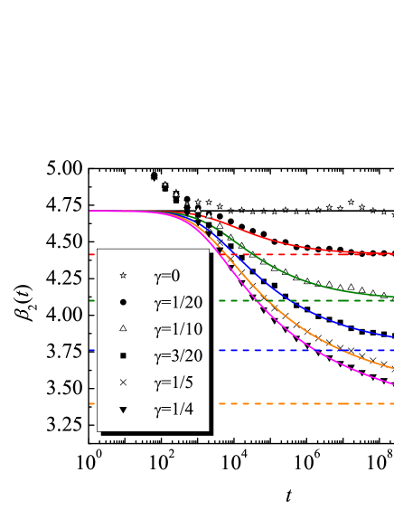
Figure 1: Kurtosis for a subdiffusive random walk with $\alpha=1/2$ and $K_{\alpha}=1/2$ on an evolving domain with power-law scale factor $a(t)=(1+t/t_{0})^{\gamma}$, for $t_{0}=10^{3}$ and $\gamma=0$, $1/20$, $1/10$, $3/20$, $1/5$, and $1/4$. Symbols represent simulations results with $10^{6}$ realisations. Numerical solutions are represented by solid lines. The value of $\beta_{2}(t)$ was computed by numerical integration of the Lagrangian fourth-order moment and subsequent division by the analytical expression of the squared Lagrangian second-order moment. Horizontal dashed lines represent the value of $\beta_{2}^{\infty}$ for each value of $\gamma$ according to equation (46). The asymptotic value for $\gamma=1/4$, $\beta_{2}^{\infty}=3$, is not shown.

In figure 1 we show simulations results for a power-law expansion $a(t)=(1+t/t_{0})^{\gamma}$ with $t_{0}=10^{3}$ and different values of $\gamma\leq\alpha/2$. The curves for $\beta_{2}(t)$ can be seen to approach the value of $\beta_{2}^{\infty}$ given by result (46). In particular, the decrease of $\beta_{2}^{\infty}$ with increasing $\gamma$ predicted by equation (46) is confirmed. The theoretical results compare very favourably with Monte-Carlo simulations at times sufficiently long to reach the diffusive regime.

In figure 2 we illustrate how the form of the propagator changes as its kurtosis evolves in time. We show the Lagrangian propagator for a power-law expansion $a(t)=(1+t/t_{0})^{\gamma}$ with $t_{0}=10^{3}$ and $\gamma=\alpha/2=1/4$ at two different times. In panel (a), we display the propagator at a comparatively short time ($t=2^{14}$). We have been able to solve the FDE computationally up to this time (details of the algorithm can be found in reference [89]). The propagator is still quite pointy at $x=0$ and thus not too different from the shape on a static domain ($\gamma=0$). In more quantitative terms, at $t=2^{14}$ the kurtosis of $W(x,t)$ is $\beta_{2}\left(2^{14}\right)\simeq 4.22$, whereas on a static domain one would have $\beta_{2}^{\mathrm{static}}\approx 4.71$. However, at the later time $t=2^{34}$—see panel (b)—our numerical Monte-Carlo simulations reveal that the sharp peak at $x=0$ evolves into a bell-shaped hump. This signals the evolution of the propagator towards the Gaussian-like state reached as $t\to\infty$. However, the kurtosis $\beta_{2}\left(t=2^{34}\right)\simeq 3.42$ at this time is still clearly distinguishable from the final value $\beta_{2}^{\infty}=3$.

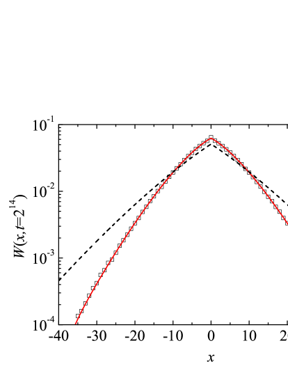
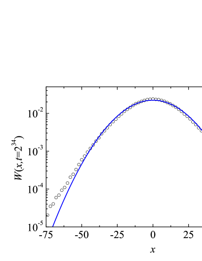
Figure 2: Logarithmic representation of the Lagrangian propagator $W(x,t)$ for a subdiffusive particle with $\alpha=1/2$ and $K_{\alpha}=1/2$. The domain growth is given by the power-law scale factor $a(t)=(1+t/10^{3})^{1/4}$. In panel (a) we show the simulations results (empty squares) for the propagator at time $t=2^{14}$, together with numerical solution of equation (25) obtained via a fractional finite-difference method [89] with spatial discretisation $\Delta x=0.1$ and time discretisation $\Delta t=0.1$ (solid line). The dashed line represents the exact solution for the static case at $t=2^{14}$. In panel (b) we show the propagator at $t=2^{34}$ obtained from simulations (empty circles), and we compare it with a Gaussian whose variance is taken to be that of the real distribution.

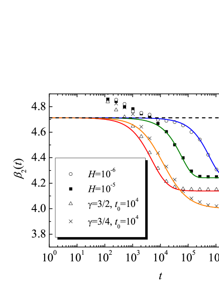
Figure 3: Kurtosis for a subdiffusive random walk with $\alpha=1/2$ and $K_{\alpha}=1/2$ on fast growing domains ($\gamma>\alpha/2$ for power-law expansions and $H>0$ for exponential expansions). The two upper curves correspond to an exponential scale factor $a(t)=\exp(Ht)$, whose logarithmic derivative is, respectively, $H=10^{-5}$ and $10^{-6}$. The two bottom curves correspond to a power-law scale factor $a(t)=(1+t/t_{0})^{\gamma}$ with $t_{0}=10^{4}$ and $\gamma=3/2$ and $3/4$, from top to bottom at $t=10^{8}$. Symbols represent simulation results from $10^{6}$ realisations. Numerical solutions are depicted by solid lines. The value of $\beta_{2}(t)$ was computed by numerical integration of the Lagrangian fourth-order moment and subsequent division by the analytical expression of the squared Lagrangian second-order moment. The dashed line depicts the value of $\beta_{2}^{\mathrm{static}}\simeq 4.71$ (cf. equation (20)).

In contrast to the case $\gamma\leq\alpha/2$ for a sufficiently fast domain growth ($\gamma>\alpha/2$) the final value of the kurtosis $\beta_{2}^{\infty}$ increases as $\gamma$ grows. As shown in reference [59], in this $\gamma$-regime the Lagrangian propagator eventually freezes and its final form is always leptokurtic ($\beta_{2}^{\infty}>3$). This also implies the long-time freeze-out of all the associated moments, which tend to finite values as $t\to\infty$. In particular, this holds for the second- and the fourth-order moments, from which the kurtosis is computed. As explained in reference [59], the physical reason for the observed freeze-out is the irrelevance of the diffusive spreading with respect to the Hubble drift at sufficiently long times. As a result of this, after a characteristic time $t_{\mathrm{char}}>t_{0}$ (see figure 3), changes in the form of the Lagrangian propagator and in the associated kurtosis become negligibly small, and the monotonic time decrease of the kurtosis saturates at a value $\beta_{2}^{\infty}\in(3,\beta_{2}^{\mathrm{static}})$. Of course, $t_{\mathrm{char}}$ will depend on both $t_{0}$ and $\gamma$. For larger values of $\gamma$, one expects a decrease of $t_{\mathrm{char}}$, since the Hubble drift becomes dominant with respect to the diffusive spreading at earlier times, and hence the saturation in Lagrangian space becomes faster. This entails a stronger memory of the tailedness displayed by the early-time propagator, and therefore a larger $\gamma$ leads to a larger $\beta_{2}^{\infty}$. Note that this is just the opposite of what happens when $0<\gamma\leq\alpha/2$. Our findings for the case $\gamma>\alpha/2$ are fully confirmed by the results shown in figure 3, which displays a comparison between theory and simulations in the long-time regime.

Summarising, Gaussian-like behaviour is only observed when $\gamma=\alpha/2$. For any other value the kurtosis of the final distribution is always $>3$, i.e., the final PDF is leptokurtic and a strong signature of the early-time PDF persists for arbitrarily long times. Note, however, that the asymptotic value $\beta_{2}^{\infty}$ does not depend on the characteristic time $t_{0}$, which only has an influence on the transient behaviour.

Of course, in the exponential case $a(t)=e^{Ht}$ with $H>0$, a freeze-out of the Lagrangian propagator also takes place. It is, however, striking that $\beta_{2}^{\infty}=3\times 2^{1-\alpha}$, regardless of the value of $H$. For any $\alpha<1$ one has $\beta_{2}^{\infty}>\beta_{2}^{\mathrm{Gaussian}}\equiv 3$, but $\beta_{2}^{\infty}<\beta_{2}^{\mathrm{static}}\equiv 3\Gamma(\alpha)\Gamma(1+\alpha)/\Gamma(2\alpha)$—see equation (20).

Results for two different values of $H>0$ are displayed in figure 3. The kurtosis $\beta_{2}(t)$ in this case is seen to approach $\beta_{2}^{\infty}$ at a time of the order of $1/H$. As already anticipated $\beta_{2}^{\infty}$ does not depend on $H$.

Of interest is also the behaviour in the case of exponential contraction, i.e., $a(t)=e^{Ht}$ with $H<0$. In this case it is easier to work in physical coordinates. In the limit $t\to\infty$ one has the asymptotic behaviour

$$\langle y^{2}\rangle_{0}\sim\frac{K_{\alpha}t^{\alpha-1}}{|H|\Gamma(\alpha)},$$ (47)

$$\langle y^{4}\rangle_{0}\sim\frac{3\times 2^{1-\alpha}(K_{\alpha})^{2}}{|H|^{1+\alpha}\Gamma(\alpha)}t^{\alpha-1}.$$ (48)

whence

$$\beta_{2}\sim 3\times 2^{1-\alpha}|H|^{1-\alpha}t^{1-\alpha}.$$ (49)

For further details of the calculations of the moments, including the use of Tauberian theorems, we refer to reference [59].

As expected, when $\alpha=1$ the kurtosis is equal to three, whereas for $\alpha<1$ the kurtosis always grows in time (in this case, it is proportional to $t^{1-\alpha}$).

Other types of contraction can also be considered. The case of power-law contraction, i.e., $a(t)=(1+t/t_{0})^{\gamma}$ with $\gamma<0$, is also covered by our formalism. The kurtosis $\beta_{2}(t)$ increases in time, until a limiting value $\beta_{2}^{\infty}$ is attained. This limiting value is still given by equation (46), which also holds for $\gamma<0$. For a given $\alpha<1$, the value of $\beta_{2}^{\infty}$ grows with increasing $|\gamma|$.

We close this subsection by noting that the observed time increase of $\beta_{2}$ for shrinking domains is likely to be related to the inversion of the direction of the Hubble drift with respect to the case of a growing domain (in uniformly shrinking domains, the Hubble drift tends to bring any two physical points closer to each other, whereas it tends to separate them in a uniformly growing domain). We actually conjecture that beyond the two cases with exponential and power-law scale factor studied here, the kurtosis of the propagator generated by subdiffusive walks with $\alpha<1$ displays a time decrease (increase) on any uniformly growing (shrinking) infinite domain.

2.4 Lévy flights

As already anticipated, in the case of Lévy flights ($\alpha=1$ and $\mu<2$) the propagator $W_{0}(x,t)$ associated with equation (23) can be explicitly obtained. One has

$$W_{0}(x,t)=\mathsf{L}_{\mu}\left(x;K_{1}^{\mu}\int_{0}^{t}a^{-\mu}(u)du\right),$$ (50)

where

$$\mathsf{L}_{\mu}(x;\sigma_{L}^{\mu})=\mathcal{F}^{-1}\left[\exp\left(-|k\sigma_{L}|^{\mu}\right)\right]$$ (51)

is a symmetric Lévy-stable density with exponent $\mu$ and scale factor $\sigma_{L}$. Note that for $\mu=2$, this Lévy density becomes a Gaussian PDF with standard deviation $\sigma=\sqrt{2}\sigma_{L}$.

By definition, the second-order moment of a Lévy flight is infinite. However, one can define a typical width as $w_{\mu}(t)\equiv C_{\mu}\sigma_{L}(t)$, where $C_{\mu}$ is a constant chosen in such a way that

$$\int_{0}^{w_{\mu}(t)}W_{0}(x,t)dx=P/2$$ (52)

holds, where $P$ is a predetermined probability.

The typical width $w_{\mu}$ will be seen to play an important role when addressing the kinetics of mixing of two initially localised Lévy pulses evolving on a growing domain (cf. section 4).

2.5 Fractional diffusion equation in physical coordinates

It is possible to obtain the PDF $W_{0}^{*}(y,t)$ to find a particle inside the interval $[y,y+dy]$ at time $t$ by noting that it is related to the PDF $W(x,t)$ for finding the particle in the corresponding interval $[x,x+dx]$, where $x=y/a(t)$. One has [59]

$$W_{0}^{*}(y,t)=\frac{W_{0}(x=y/a,t)}{a(t)}.$$ (53)

This implies the three relations

$$\left.\frac{\partial W_{0}}{\partial t}\right|_{x}=a\left.\frac{\partial W_{0}^{*}}{\partial t}\right|_{y}+\dot{a}\left.\frac{\partial(yW_{0}^{*})}{\partial y}\right|_{t},$$ (54)

$$\partial W_{0}/\partial x|_{t}=a^{2}\partial W_{0}^{*}/\partial y|_{t},$$ (55)

and

$$\nabla^{\mu}_{x}W_{0}(x,t)=a^{1+\mu}\nabla^{\mu}_{y}W_{0}^{*}(y,t).$$ (56)

Inserting relations (54) to (56) into equation (23) one eventually finds the sought equation

$$\frac{\partial W_{0}^{*}(y,t)}{\partial t}=-\frac{\dot{a}(t)}{a(t)}\frac{\partial}{\partial y}\left[yW_{0}^{*}(y,t)\right]+K_{\alpha}^{\mu}\nabla^{\mu}_{y}a(t)^{-1}\left\{\,{}_{0}D_{t}^{1-\alpha}\left[a(t)W_{0}^{*}(a(t)x,t)\right]\right\}_{x\to y/a(t)}.$$ (57)

In the case $\mu=2$ it is possible to directly obtain the behaviour of the physical moments $\langle y^{n}(t)\rangle\equiv\int_{-\infty}^{\infty}y^{n}W_{0}^{*}(y,t)dy$ by multiplication of equation (57) with $y^{n}$ and subsequent integration over $y$. This yields a hierarchy of differential equations for the physical moments.

3 CTRW in a velocity field

The diffusion of a particle in a uniform velocity field can be regarded as the motion of a random walker dragged by a fluid flowing with velocity $\vec{v}$ with respect the laboratory reference frame $\mathcal{S}_{L}$ (for simplicity, the velocity $\vec{v}$ will hereafter be assumed to be stationary unless otherwise specified). An example would be a frog performing random jumps with statistically distributed waiting times on a wooden log that is longitudinally floating downstream on a river. On a more microscopic scale one could imagine a tracer particle subdiffusing in a hydrogel that itself is slowly streamed in a fluidic device.

Let us now introduce a second reference frame $\mathcal{S}_{0}$ in which the deterministic contribution of the velocity field is subtracted from the overall particle motion, i.e., a frame which follows the fluid that drags the particle along. Clearly, $\mathcal{S}_{L}$ moves with velocity $-\vec{v}$ with respect to $\mathcal{S}_{0}$. Let us respectively denote by $W_{0}(\vec{y},t)$ and $W(\vec{y},t)$ the walker’s PDF in $\mathcal{S}_{0}$ and $\mathcal{S}_{L}$. On a static domain the relation between both PDFs will be given by the Galilean transformation $W(\vec{y},t)=W_{0}(\vec{y}-\vec{v}t,t)$. In particular one has

$$W(y,t)=W_{0}(y-vt,t)$$ (58)

in one dimension. In Fourier-Laplace space equation (58) becomes

$$W(k,u)=W_{0}(k,u+ikv).$$ (59)

In the case of a growing domain the particle is not only advected by the velocity field but also experiences an additional drift as it is dragged by the physical medium (i.e., the aforementioned Hubble drift). Recalling the previous example of a hopping frog on a log floating downstream, one might wonder what the equation of motion of the frog would be if the log were replaced by a linear rubber strip that expands uniformly with a certain scale factor. Before providing the answer to this question, we will first address the simpler case of a static domain, as done in section 2.

3.1 Static domain

From equations (59) and (6) one finds

$$W(k,u)=\frac{W(k,0)}{u+ivk+K_{\alpha}^{\mu}|k|^{\mu}(u+ivk)^{1-\alpha}},$$ (60)

or, equivalently,

$$(u+ivk)W(k,u)-W(k,0)=-K_{\alpha}^{\mu}|k|^{\mu}(u+ivk)^{1-\alpha}W(k,u),$$ (61)

whence the Galilei-invariant (GI) advection-diffusion equation

$$\left(\frac{\partial}{\partial t}+v\frac{\partial}{\partial y}\right)W(y,t)=K_{\alpha}^{\mu}\nabla^{\mu}_{y}\left(\frac{\partial}{\partial t}+v\frac{\partial}{\partial y}\right)^{1-\alpha}W(y,t)$$ (62)

follows. The operator $\left(\partial_{t}+v\,\partial_{y}\right)^{1-\alpha}$ is the fractional material derivative introduced by Sokolov and Metzler [90]. It is defined by

$$\mathscr{F}\mathscr{L}\left[\left(\frac{\partial}{\partial t}+v\frac{\partial}{\partial y}\right)^{1-\alpha}W(y,t)\right]=(u+ivk)^{1-\alpha}W(k,u).$$ (63)

From this expression and from relation (9) one can see that the fractional material derivative reduces to the GL derivative if $v=0$. As mentioned in the Introduction, the GI fractional advection-diffusion equation (62) for $\mu=2$ was recently obtained by Cairoli et al. [85]. While the standard material derivative, corresponding to the limit $\alpha=1$ reflects the GI of a standard physical system, the power $(1-\alpha)$ reflects the spatio-temporal coupling in a waiting time-random walk scenario with a constant relocation speed $v$.

The fractional derivative in direct (position-time) space is [91]

$$\left(\frac{\partial}{\partial t}+v\frac{\partial}{\partial y}\right)^{1-\alpha}=\frac{1}{\Gamma(\alpha)}\left(\frac{\partial}{\partial t}+v\frac{\partial}{\partial y}\right)\int_{0}^{t}d\tau\frac{W(y-v(t-\tau),\tau)}{(t-\tau)^{1-\alpha}}.$$ (64)

Here, it is assumed that $W(k,t)$ satisfies the condition (11) of good behaviour at $t=0$.

The fractional material derivative can be rewritten in terms of the RL integral in the convenient form

$$\left(\frac{\partial}{\partial t}+v\frac{\partial}{\partial y}\right)^{1-\alpha}W(y,t) = \left(\frac{\partial}{\partial t}+v\frac{\partial}{\partial y}\right)\left[\,{}_{0}D_{t}^{-\alpha}W(y+vt,t)\right]_{y\to y-vt}$$ (65)

$$= \left(\frac{\partial}{\partial t}+v\frac{\partial}{\partial y}\right)\left[\,{}_{0}D_{t}^{-\alpha}W_{0}(y,t)\right]_{y\to y-vt}.$$

In this way the GI advection-diffusion equation (62) becomes

$$\left(\frac{\partial}{\partial t}+v\frac{\partial}{\partial y}\right)W(y,t)=K_{\alpha}^{\mu}\nabla^{\mu}_{y}\left(\frac{\partial}{\partial t}+v\frac{\partial}{\partial y}\right)\left[\,{}_{0}D_{t}^{-\alpha}W_{0}(y,t)\right]_{y\to y-vt}.$$ (66)

Note that in the above expression the time fractional derivative is applied to $W_{0}$, which corresponds to the particle distribution in the reference frame $\mathcal{S}_{0}$. This frame moves by a distance $vt$ during the time $t$. As a result of this the evaluation point for the derivative is shifted by the same quantity.

Finally, it should be noted that the propagator (60) and the corresponding FDAE (66) differ from those considered in references [92] and [93]. In particular, for $\mu=2$, the propagator studied in these works can reach non-physical negative values with moments that are only correct up to order two.

3.2 Growing domain

We continue to assume that the particle is subject to the influence of a constant velocity field (the velocity measured with respect to the laboratory frame $\mathcal{S}_{L}$ is $v$). As in the case of a symmetric walk it is convenient to work in Lagrangian coordinates. If the domain expands uniformly with the scale factor $a(t)$, the Lagrangian distance travelled by the reference frame $\mathcal{S}_{0}$ (the frame moving with velocity $v$ with respect to $\mathcal{S}_{L}$) during the time $t$ is

$$\Lambda(t)=\int_{0}^{t}\frac{v}{a(t^{\prime})}\,dt^{\prime}\equiv\int_{0}^{t}\nu(t^{\prime})\,dt^{\prime}\equiv vT(t).$$ (67)

Here, the transformed time $T(t)$ replaces the physical time $t$ as a result of the difference between the Lagrangian distance $\Lambda(t)$ travelled by $\mathcal{S}_{0}$ and the distance $vt$ that it would cover on a static domain. For instance, an exponential growth $a(t)=\exp(Ht)$ with $H>0$ yields,

$$T(t)=\frac{1-\exp(-Ht)}{H},$$ (68)

whereas a power-law growth $a(t)=(1+t/t_{0})^{\gamma}$ gives

$$T(t)=\frac{t_{0}}{\gamma-1}\left[1-\left(\frac{t}{t_{0}}\right)^{1-\gamma}\right],\qquad\gamma\neq 1$$ (69)

and

$$T(t)=t_{0}\ln\left(1+\frac{t}{t_{0}}\right),\qquad\gamma=1.$$ (70)

Thus, for a sufficiently fast growth (exponential or power-law with $\gamma>1$) one has an asymptotic finite value $T_{\infty}\equiv T(t\to\infty)$, and correspondingly the asymptotic Lagrangian distance $\Lambda_{\infty}\equiv\Lambda(t\to\infty)$ is also finite.

The PDF $W(x,t)$ in the laboratory frame $\mathcal{S}_{L}$ is just the PDF $W_{0}(z,t)$ in the comoving reference frame $\mathcal{S}_{0}$, but with the shifted position $z=x-\Lambda(t)$. In other words,

$$W(x,t)=W_{0}(x-\Lambda(t),t).$$ (71)

In figure 4 the above relation is illustrated for a stretching domain with $a(t)=(1+t/10^{3})^{1/8}$ by comparing simulations results for $W_{0}$ and $W$. The Lagrangian propagators are also compared with the corresponding ones for the case of a static domain. Note that the width of the propagator is decreased with respect to the static case, since the jump length measured in Lagrangian coordinates is divided by $a(t)$.

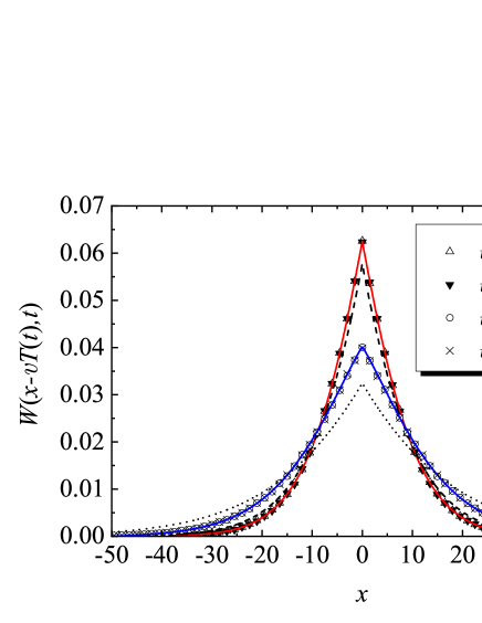
Figure 4: Lagrangian propagators for a subdiffusive random walk with $\mu=2$, $\alpha=1/2$, and $K_{\alpha}=1/2$. The domain growth is given by a power-law scale factor $a(t)=(1+t/10^{3})^{1/8}$. We display cases with $v=0$ (zero field) and $v=1$. Symbols depict simulations results at times $t=10^{4}$ and $t=10^{5}$ for the case $v=0$ and $v=1$ (see legend). Solid lines represent numerical solutions of equation (25) at these times (the temporal and spatial steps are, respectively, $\Delta t=t/10^{5}$ and $\Delta x=0.1$). The broken lines are the exact solutions at $t=10^{4}$ (dashed) and $t=10^{5}$ (dotted) for a static domain.

Now, as we already know from section 2, $W_{0}(x,t)$ satisfies relation (23). Since $\Lambda(t)$ may be a complicated function of $t$, in general no relationship between the Fourier-Laplace transforms of $W(x,t)$ and $W_{0}(x,t)$ similar to equation (59) can be obtained from result (71). Therefore, we can no longer use the straightforward procedure of section 2 to derive the FDAE that we seek. For this reason, we will follow a different path involving equations (23), (66), and (71).

In view of equations (66) and (23) a reasonable guess for the FDAE is

$$\left(\frac{\partial}{\partial t}+\nu\frac{\partial}{\partial x}\right)W(x,t)=\frac{K_{\alpha}^{\mu}}{a^{\mu}(t)}\nabla^{\mu}_{x}\left[{}_{0}D_{t}^{1-\alpha}W_{0}(x,t)\right]_{x\to x-\Lambda(t)},$$ (72)

since $\Lambda(t)$ and $vt$ in equations (72) and (66) are, respectively, the displacement in the laboratory frame $\mathcal{S}_{L}$ of the comoving frame $\mathcal{S}_{0}$ during the time $t$. We confirm that equation (72) is indeed the correct FDAE by showing that $W(x,t)$, as given by equation (71), satisfies relation (72). First, let us evaluate the left-hand side of equation (72),

$$\left(\frac{\partial}{\partial t}+\nu\frac{\partial}{\partial x}\right)W(x,t)=\left(\frac{\partial}{\partial t}+\nu\frac{\partial}{\partial x}\right)W_{0}(x-\Lambda(t),t)=\left.\frac{\partial W_{0}}{\partial t}\right|_{x-\Lambda(t)}.$$ (73)

Next, we evaluate the right-hand side of equation (72),

$$\frac{K_{\alpha}^{\mu}}{a^{\mu}(t)}\nabla^{\mu}_{x}\left[{}_{0}D_{t}^{1-\alpha}W_{0}(x,t)\right]_{x\to x-\Lambda(t)} = \left[\frac{K_{\alpha}^{\mu}}{a^{\mu}(t)}\nabla^{\mu}_{x}\,{}_{0}D_{t}^{1-\alpha}W_{0}(x,t)\right]_{x\to x-\Lambda(t)}$$ (74)

$$= \left.\frac{\partial W_{0}}{\partial t}\right|_{x-\Lambda(t)},$$

where, in the last step, equation (23) was taken into account. Comparing equation (73) with (74) we conclude that $W(x,t)=W_{0}(x-\Lambda(t),t)$ indeed satisfies relation (72). Defining

$$\left(\frac{\partial}{\partial t}+\nu\frac{\partial}{\partial x}\right)^{1-\alpha}W(x,t)\equiv\left(\frac{\partial}{\partial t}+\nu\frac{\partial}{\partial x}\right)\frac{1}{\Gamma(\alpha)}\int_{0}^{t}d\tau\frac{W\left(x+\Lambda(\tau)-\Lambda(t),\tau\right)}{(t-\tau)^{1-\alpha}},$$ (75)

the FDAE (66) for a uniformly growing domain can be rewritten in a way similar to equation (62),

$$\left(\frac{\partial}{\partial t}+\nu\frac{\partial}{\partial x}\right)W(x,t)=\frac{K_{\alpha}^{\mu}}{a^{\mu}(t)}\nabla^{\mu}_{x}\left(\frac{\partial}{\partial t}+\nu\frac{\partial}{\partial x}\right)^{1-\alpha}W(x,t).$$ (76)

Equation (76), or equivalently equation (72) (see just below), is one of the main results of this paper.

Comparing equations (72) and (76) one can see that both are equivalent if

$$\left(\frac{\partial}{\partial t}+\nu\frac{\partial}{\partial x}\right)^{1-\alpha}W(x,t)=\left[{}_{0}D_{t}^{1-\alpha}W_{0}(x,t)\right]_{x\to x-\Lambda(t)}.$$ (77)

In order to prove this we first note that equation (75) can be rewritten as (see equation (12))

$$\left(\frac{\partial}{\partial t}+\nu\frac{\partial}{\partial x}\right)^{1-\alpha}W(x,t)=\left(\frac{\partial}{\partial t}+\nu\frac{\partial}{\partial x}\right)\left[{}_{0}D_{t}^{-\alpha}W(x+\Lambda(t),t)\right]_{x\to x-\Lambda(t)}.$$ (78)

Conversely, for any differentiable function $G(x,t)$, one has

$$\left(\frac{\partial}{\partial t}+\nu\frac{\partial}{\partial x}\right)\left[G(x,t)\right]_{x\to x-\Lambda(t)}=\left(\frac{\partial}{\partial t}+\nu\frac{\partial}{\partial x}\right)G(x-\Lambda(t),t)$$

$$=\left.\frac{\partial G}{\partial t}\right|_{x-\Lambda(t)}-\frac{\partial\Lambda(t)}{\partial t}\left.\frac{\partial G}{\partial x}\right|_{x-\Lambda(t)}+\nu\left.\frac{\partial G}{\partial x}\right|_{x-\Lambda(t)}=\left.\frac{\partial G}{\partial t}\right|_{x-\Lambda(t)}.$$ (79)

Taking $G(x,t)=\,_{0}D_{t}^{-\alpha}W(x+\Lambda(t),t)$ and assuming that $(d/dt){{}_{0}}D_{t}^{-\alpha}=\,_{0}D_{t}^{1-\alpha}=\,_{0}\mathcal{D}_{t}^{1-\alpha}$ (see equation (10)), one finds that the right hand side of equations (77) and (78) coincide, implying that relation (77) indeed holds.

Even though the velocity $v$ has been assumed to be constant, it is worth noting that equations (72) and (76) still hold when the reference frame $\mathcal{S}_{0}$ moves with a time-dependent velocity with respect to $\mathcal{S}_{L}$. In this case, one simply replaces $\nu=v/a(t)$ with $\nu=v(t)/a(t)$.

We close this section by deriving the FDAE in terms of the physical coordinate $y$. The derivation proceeds along the same lines as in the field-free case (cf. section 2). The relations (53) to (56) for this latter case are completely analogous to the equations relating $W^{*}(y,t)$ and $W(x,t)$ in the presence of the velocity field. Indeed, one has

$$W^{*}(y,t)=\frac{W(x=y/a,t)}{a(t)},$$ (80)

and, correspondingly,

$$\left.\frac{\partial W}{\partial t}\right|_{x}=a\left.\frac{\partial W^{*}}{\partial t}\right|_{y}+\dot{a}\left.\frac{\partial(yW^{*})}{\partial y}\right|_{t},$$ (81)

as well as

$$\left.\frac{\partial W}{\partial x}\right|_{t}=a^{2}\left.\frac{\partial W^{*}}{\partial y}\right|_{t},$$ (82)

and

$$\nabla^{\mu}_{x}W(x,t)=a^{1+\mu}\,\nabla^{\mu}_{y}W^{*}(y,t).$$ (83)

Inserting equations (80) to (83) into (72) and taking into account equation (71) one eventually obtains the result

$$\frac{\partial W^{*}}{\partial t}=-\frac{\partial}{\partial y}\left[\left(\frac{\dot{a}}{a}y+a\nu\right)W^{*}(y,t)\right]+K_{\alpha}^{\mu}\nabla^{\mu}_{y}{{}_{0}}P_{t}^{1-\alpha}W^{*}(y,t),$$ (84)

where

$$_{0}P_{t}^{1-\alpha}W^{*}(y,t)=\frac{1}{a}\left\{\,{}_{0}D_{t}^{1-\alpha}\left[aW^{*}(ax+a\Lambda,t)\right]\right\}_{x=(y-\Lambda)/a}.$$ (85)

Let us once more recall that equation (84) holds for well-behaved functions $W^{*}(y,t)$. Strictly speaking, the RL-fractional derivative therein must be replaced with the GL-fractional derivative ${}_{0}{\cal D}_{t}^{1-\alpha}$, and consequently, ${}_{0}P_{t}^{1-\alpha}$ must also be replaced with the corresponding operator, defined via the equation

$$_{0}{\cal P}_{t}^{1-\alpha}W^{*}(y,t)=\frac{1}{a}\left\{\,{}_{0}{\cal D}_{t}^{1-\alpha}\left[aW^{*}(ax+a\Lambda,t)\right]\right\}_{x=(y-\Lambda)/a}.$$ (86)

3.3 Moments of the propagator

From the exact relationship (71) one can easily find the moments $\langle x^{n}\rangle$ of $W$ in terms of the moments $\langle x^{n}\rangle_{0}$ of $W_{0}$. One has

$$\langle x^{n}\rangle=\int(z+\Lambda)^{n}W_{0}(z,t)=\sum_{m=0}^{n}{n\choose m}\Lambda^{n-m}\langle x^{m}\rangle_{0}.$$ (87)

Restricting ourselves to the case $\mu=2$ and $0<\alpha\leq 1$ (subdiffusive case), the second- and fourth-order moments of the PDF are respectively given by equations (26) and (38). By symmetry, odd moments vanish trivially, $\langle x^{2n+1}\rangle_{0}\equiv 0$. Taking all this into account in equation (87) we find explicit expressions for the first four Lagrangian moments:

$$\langle x\rangle=\Lambda(t),$$ (88)

$$\langle x^{2}\rangle=\Lambda^{2}(t)+\frac{2K_{\alpha}}{\Gamma(\alpha)}\int_{0}^{t}d\tau\frac{\tau^{\alpha-1}}{a^{2}(\tau)}$$ (89)

$$\langle x^{3}\rangle=\Lambda^{3}(t)+\frac{6K_{\alpha}}{\Gamma(\alpha)}\Lambda(t)\int_{0}^{t}d\tau\frac{\tau^{\alpha-1}}{a^{2}(\tau)}$$ (90)

$$\langle x^{4}\rangle=\Lambda^{4}(t)+\frac{12K_{\alpha}}{\Gamma(\alpha)}\Lambda^{2}(t)\int_{0}^{t}d\tau\frac{\tau^{\alpha-1}}{a^{2}(\tau)}+24\frac{(K_{\alpha})^{2}}{\Gamma(\alpha)}\int_{0}^{t}\frac{d\tau}{a^{2}(\tau)}\,_{0}D_{\tau}^{-\alpha}\frac{\tau^{\alpha-1}}{a^{2}(\tau)}.$$ (91)

Focusing on the first two equations, equation (88) tells us that the first moment $\langle x\rangle$ is simply given by the deterministic shift, i.e., the Lagrangian distance $\Lambda(t)$ travelled by ${\cal S}_{0}$ after a time $t$. Conversely, equation (89) implies that $\langle x^{2}\rangle_{0}-\langle x\rangle_{0}^{2}$ equals $\langle x^{2}\rangle-\langle x\rangle^{2}$, i.e., the variance in ${\cal S}_{0}$ is the same as in ${\cal S}_{L}$. Thus, regardless of the value of $\alpha$ the dispersion properties of the random walk are not affected by the velocity field. In contrast, in the case of a constant external force [61] this only holds when the particles are Brownian ($\alpha=1$). As soon as $0<\alpha<1$, the dispersion properties are altered both on a static domain [23] and on a growing domain [61].

It is instructive to check that the expressions for the moments obtained above can be directly recovered from equation (76). In order to deduce equations (88) to (90) from equation (76) we first multiply this latter equation with $x^{n}$ and subsequently integrate over space. We are then left with the hierarchy

$$\frac{d\langle x^{n}\rangle}{dt}-n\nu\langle x^{n-1}\rangle=\frac{K_{\alpha}}{\Gamma(\alpha)a^{2}(t)}\left(\frac{\partial}{\partial t}\int_{0}^{t}d\tau\frac{I^{(n)}_{2}}{(t-\tau)^{1-\alpha}}+\nu\int_{0}^{t}d\tau\frac{I^{(n)}_{3}}{(t-\tau)^{1-\alpha}}\right),$$ (92)

where

$$I^{(n)}_{m}=\int_{-\infty}^{\infty}dxx^{n}\frac{\partial^{m}}{\partial x^{m}}W(x-\Lambda(t)+\Lambda(\tau),\tau).$$ (93)

Performing the change of variable $z=x-\Lambda(t)+\Lambda(\tau)$ in this integral, using the binomial expansion for $z^{n}$, and integrating by parts, one finally obtains

$$\frac{d\langle x^{n}\rangle}{dt}=n\nu\langle x^{n-1}\rangle+\frac{K_{\alpha}}{\Gamma(\alpha)a^{2}(t)}\sum_{j=2}^{n}{n\choose j}j(j-1)\left(\frac{d}{dt}J^{(n)}_{j,2}-\nu(j-2)J^{(n)}_{j,3}\right),$$ (94)

where

$$J^{(n)}_{j,m}=\int_{0}^{t}d\tau\frac{\left[\Lambda(t)-\Lambda(\tau)\right]^{n-j}}{(t-\tau)^{1-\alpha}}\langle x^{j-m}(\tau)\rangle.$$ (95)

For $n=1$ equation (94) becomes $d\langle x\rangle/dt=\nu$, and equation (88) follows immediately. For $n=2$ relation (94) becomes

$$\frac{d\langle x^{2}\rangle}{dt}=2\nu\langle x\rangle+\frac{2K_{\alpha}}{\Gamma(\alpha)a^{2}(t)}\frac{d}{dt}J_{2,2}^{(2)}.$$ (96)

From this equation and from result (88) one immediately finds equation (89) by taking into account that $dJ_{2,2}^{(2)}/dt=t^{\alpha}/\alpha$.

We now proceed to derive equation (90) from result (94). For $n=3$, relation (94) can be written as

$$\frac{d\langle x^{3}\rangle}{dt}=3\nu\langle x^{2}\rangle+\frac{6K_{\alpha}}{\Gamma(\alpha)a^{2}(t)}t^{\alpha-1}\Lambda(t)$$ (97)

after a straightforward calculation making use of equation (88). Inserting equation (89) into (97) one obtains

$$\frac{d\langle x^{3}\rangle}{dt}=3\nu\Lambda^{2}+\frac{6K_{\alpha}}{\Gamma(\alpha)}\frac{d}{dt}\left[\Lambda\int_{0}^{t}\frac{\tau^{\alpha-1}}{a^{2}(\tau)}d\tau\right].$$ (98)

Equation (90) then follows immediately from (98).

The validity of result (91) for the fourth-order moment can also be corroborated in a similar way. The calculation is straightforward but not shown here explicitly.

4 Mixing of diffusive pulses

We now proceed to study the influence of a velocity field on the mixing properties of two diffusive pulses on a uniformly growing one-dimensional domain. We consider both cases of normal and anomalous diffusion. For convenience, our analysis will be carried out in Lagrangian coordinates.

As mentioned in the Introduction, mixing properties are crucial to understand encounter-controlled reactions involving pairwise interactions, as originally modelled by Smoluchowski [95]. In biological cells, for instance, monomers of regulatory proteins meet diffusively and form dimers [96], and the dimer then diffuses to its designated binding site on the genome or a DNA plasmid [97, 98]. Analogous processes need to run off in vesicles designed as artificial cells [99]. In the case of particles advected by the growing domain, for instance, by the expanding cytoskeleton in a living biological cell or compartments in growing vesicles [99], it is intuitively clear that the associated Hubble drift will reduce diffusional mixing and thereby decrease the reaction rate [64, 65, 66]. For sufficiently fast domain growth the lack of mixing stems from a premature freezing of the pulse propagators [63, 64, 65, 66], since the Lagrangian step lengths become increasingly short in the course of time (for a contracting domain, the Lagrangian steps become larger and one has the opposite effect).

In our problem, the random motion of each pulse is not only subject to a Hubble drift, but also to an additional drift arising from the velocity field. In order to formulate the problem in the most general form, we will assume that each diffusing particle “feels” a different velocity field. In other words, the force underlying this velocity field can be thought of as being able to discriminate each particle by a distinctive property. For instance, if the physical origin of the force is an electric field acting on charged, overdamped diffusive particles, then this property will be the sign and absolute value of their electric charge. In the particular case where both particles have the same charge, they will experience the same biasing force, and the mixing problem will be equivalent to its zero-field counterpart, save for a coordinate shift. In the biological context, we could be thinking of growing neuron cells, in which messenger RNA molecules are shuttled along by molecular motors [83]. Depending on the orientation of the molecular track these motors are walking, their direction may be towards either extremity of the pseudo-one-dimensional cell.

More specifically, consider two walkers labelled with indices $1$ and $2$. Let $x_{0}^{(1)}$ and $x_{0}^{(2)}$ denote their initial positions. Without loss of generality we assume that $x_{0}^{(1)}<x_{0}^{(2)}$. Owing to the external force acting on each walker, the maxima are shifted with respect to their initial positions as the pulses associated with each walker widen. Correspondingly, one has $x_{M}^{(1)}=x_{0}^{(1)}+v^{(1)}T(t)$ and $x_{M}^{(2)}=x_{0}^{(2)}+v^{(2)}T(t)$. The velocities $v^{(1)}$ and $v^{(2)}$ will hereafter be considered to be constant for the sake of simplicity.

The two-pulse PDF can be written as a normalised linear combination of the propagators for the respective initial conditions, i.e.,

$$W(x,t)=\frac{1}{2}\left[W_{0}^{(1)}(x-x_{0}^{(1)}-v^{(1)}T(t),t)+W_{0}^{(2)}(x-x_{0}^{(2)}-v^{(2)}T(t),t)\right].$$ (99)

Here, one encounters the difficulty that if at least one of the particles is subdiffusive, its propagator is not known, and hence its contribution to the joint PDF is also unknown. Nevertheless, it is possible to carry out a semiquantitative study of particle mixing on the basis of the second-order moments. To this end, let us first introduce the Lagrangian half-width of a zero-field single-particle propagator as

$$w(t)=2\sqrt{\langle x^{2}\rangle_{0}-\langle x\rangle_{0}^{2}}.$$ (100)

Let us further define two characteristic points $x_{C}^{(1)}(t)=x_{M}^{(1)}+w^{(1)}(t)$ and $x_{C}^{(2)}(t)=x_{M}^{(2)}-w^{(2)}(t)$ where, following the notation of equation (100), $w^{(1,2)}(t)>0$ denotes the Lagrangian half-width of the symmetric propagator $W_{0}^{(1,2)}(x,t)$. Mixing after a time $t$ will be considered to be weak (in a statistical sense) if $x_{C}^{(2)}(t)$ remains to the right of $x_{C}^{(1)}(t)$, i.e., if the characteristic distance $d_{C}(t)\equiv x_{C}^{(2)}(t)-x_{C}^{(1)}(t)$ remains $>0$. In other words, at a time $t$, one has weak mixing if

$$x_{0}^{(2)}-x_{0}^{(1)}>\left[v^{(1)}-v^{(2)}\right]T(t)+w^{(1)}(t)+w^{(2)}(t).$$ (101)

In contrast, when

$$x_{0}^{(2)}-x_{0}^{(1)}<\left[v^{(1)}-v^{(2)}\right]T(t)+w^{(1)}(t)+w^{(2)}(t)$$ (102)

we will simply speak about “mixing”. Similarly, if “$<$” can be replaced with “$\ll$” in equation (102) we will speak about “strong mixing”. The last two terms on the right-hand side are positive and independent of the respective velocities. Therefore, for a given set of diffusive properties, the mixing behaviour depends on the first term, which is influenced by the relative velocity $v^{(1)}-v^{(2)}$ and by the scale factor $a(t)$ entering the definition of $T(t)$. Clearly, a positive (negative) relative velocity favours (hinders) mixing, as is the case in the particular case of a static domain (this latter case is recovered by setting $T(t)\equiv t$).

Note, however, that the domain growth introduces a key difference in the behaviour. On a static domain the strong mixing condition is always fulfilled provided that one waits long enough, irrespective of whether the diffusive pulses are normal or anomalous (mixing becomes maximal when both pulse peaks overlap, i.e., when the distance $d_{M}\equiv x_{M}^{(2)}-x_{M}^{(1)}$ between the two peaks vanishes). However, for a given initial pulse separation and relative velocity, it is intuitively clear that a sufficiently fast domain growth may freeze both pulses before their mixing becomes significant. More precisely, for $v^{(1)}>0$ and $v^{(2)}<0$, one has weak mixing at arbitrarily long times if

$$x_{0}^{(2)}-x_{0}^{(1)}>\left[v^{(1)}-v^{(2)}\right]T_{\infty}+w^{(1)}_{\infty}+w^{(2)}_{\infty},$$ (103)

where $T_{\infty}\equiv\lim_{t\to\infty}T(t)<\infty$ and $w^{(1,2)}_{\infty}=\lim_{t\to\infty}w^{(1,2)}(t)<\infty$ are the long-time asymptotic values of the half-widths. Thus, a sufficiently fast domain growth favours the localisation of the Lagrangian propagators about the respective initial conditions, thereby preventing that the memory of the latter is eventually lost by mixing.

In terms of physical coordinates, the situation described by equation (103) corresponds to the case when the Hubble drift is so strong that the pulses separate from each other at a rate much faster than the typical growth rate of their half-widths. Therefore, the overlap of both pulses remains negligibly small at all times.

In what follows, we focus on the case of a set of two particles with identical diffusive properties ($w\equiv w^{(1)}=w^{(2)}$) but subject to opposite drift velocities $v\equiv v^{(1)}=-v^{(2)}$. Without loss of generality the midpoint between the two pulse peaks will be chosen as the origin, i.e., $x_{0}\equiv x_{0}^{(2)}=-x_{0}^{(1)}$.

4.1 Normal diffusion and subdiffusion

When both particles are normal-diffusive ($\alpha=1$) or subdiffusive ($0<\alpha<1$) the variance $\langle x^{2}(t)\rangle_{0}$ is well-defined and can be used to estimate $w(t)$.

In order to study the mixing kinetics the parameter $P$ in equation (52) should be chosen large enough to ensure significant mixing as soon as both tails overlap. In general, for a given value of $P$ the corresponding value of $C_{\mu}$ (as well as the associated characteristic width $w_{\mu}(t)=C_{\mu}\sigma_{L}(t)$) must be computed numerically. However, for the Gaussian case $\mu=2$ one can obtain an analytic expression, namely, $C_{2}=2\mathrm{erf}^{-1}(P)$. This result is in agreement with what we had already anticipated for the Brownian case since, for a Gaussian distribution, the probability that a particle is found within an interval of half-width $w(t)=2\sigma(t)=2\sqrt{2}\sigma_{L}(t)$ is $P=0.9545$, i.e., precisely the value which follows from the relation $\mathrm{erf}^{-1}(P)=\sqrt{2}$.

In the case of two Gaussian pulses with identical diffusive properties and opposite drift velocities this last result implies that when the weak mixing condition (101) holds the overlap of both tails as given by

$$\int_{-\infty}^{x_{C}^{(1)}}W_{0}^{(2)}(x,t)dx+\int_{x_{C}^{(2)}}^{\infty}W_{0}^{(1)}(x,t)dx$$ (104)

remains below $5\%$ at all times.

	$\gamma<\alpha/2$	$\gamma=\alpha/2$	$\alpha/2<\gamma<1$	$\gamma=1$	$\gamma>1$
$T$	$t^{1-\gamma}$	$t^{1-\gamma}$	$t^{1-\gamma}$	$\ln t$	$\mathrm{const.}$
$w$	$t^{(\alpha-2\gamma)/2}$	$\sqrt{\ln t}$	$\mathrm{const.}$	$\mathrm{const.}$	$\mathrm{const.}$

Table 1: Asymptotic long-time behaviour of $T(t)$ and $w(t)$ for a power-law scale factor with characteristic exponent $\gamma$. The results for $T(t)$ and $w(t)$ stem, respectively from the long-time behaviours of equations (68) and (100).

For a power-law scale factor $a(t)\sim t^{\gamma}$ the different possible subcases are given in Table 1. From this table one concludes that for $v=0$ and $x_{0}\ll w_{\infty}$ strong mixing does not occur when $\gamma>\alpha/2$. However, a nonzero value of $v$ may completely change this scenario and bring about strong mixing for sufficiently long times. For $v>0$, when $\alpha/2<\gamma\leq 1$, one has $T_{\infty}=\infty$, implying that the crossing of the two maxima will eventually occur with certainty. In contrast, when the domain growth is fast enough to ensure that $T_{\infty}<\infty$ the propagator evolves towards a steady state. In this latter case strong mixing will never take place if it has not already occurred by the characteristic time $t_{C}$ at which $W(x,t_{C})$ can be considered to be practically indistinguishable from $W(x,\infty)$. According to equation (102) strong mixing may be observed at a finite time $t$ if the initial separation distance is small enough—more precisely, if $x_{0}\ll vT(t)+w(t)$ holds.

Figure 5 displays the temporal evolution of two subdiffusive pulses ($\alpha=1/2$) on a growing domain with scale factor $a(t)=(1+t/10^{3})^{3/4}$. Since $\gamma>\alpha/2$ we can see that the probability of overlap grows in time. However, the respective pulse widths remain almost stationary throughout the time window spanned by the represented set of plots (the length of this window is $\sim 10t_{0}$). Thus, we conclude that in the present case mixing is driven by the opposed velocity fields rather than by the spreading of the pulses. The maximum overlap probability is attained after a time $t_{M}$, corresponding to the crossing of both pulses, i.e., to a vanishing peak separation $d_{M}(t_{M})=0$. This characteristic time can be obtained from the solution of the implicit equation $x_{0}=vT(t_{M})$. Only at this specific time $t_{M}$ does the PDF correspond to the zero field solution for a single particle, $W(x,t_{M})=W_{0}(x,t_{M})$.

For a fixed time $t=10^{4}$ figure 6 displays a series of snapshots of the Lagrangian propagator corresponding to different values of $v$. For the chosen value of the domain growth exponent ($\gamma=1/2$) and of the anomalous diffusion exponent $\alpha$ the inequality $1/4=\alpha/2<\gamma<1$ holds, and so the mixing is once again driven by the relative velocity term. As in the static case, increasing $v$ results in enhanced mixing. For the chosen parameter set the degree of mixing at a given time is maximised by the velocity value $v=0.162$. For this precise value, $d_{M}(t=10^{4})=0$, i.e., one has a single-hump propagator.

Finally in figure 7 we study a case where the domain growth is so fast ($\gamma=2$) that mixing is absent at all times. As one can see, the pulse widths remain practically the same at all times, and the deterministic displacement of the pulse peaks is greatly slowed down by the domain growth, until both pulses become almost stationary.

The theoretical curves in figures 5-7 (obtained by the numerical integration of the FDE) were corroborated by CTRW simulations. As expected, a significant discrepancy occurs at short times, since the number of steps taken by the random walker is not large enough to reach the diffusive limit (see also reference [23]). At longer times the agreement is excellent.

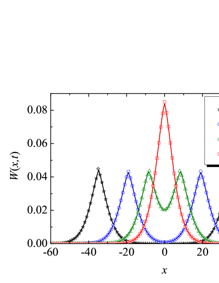
Figure 5: Lagrangian propagator at times $t=10^{4}$, $2\times 10^{4}$, $3\times 10^{4}$, and $4\times 10^{4}$, for two subdiffusive pulses that drift in opposite directions. Parameter values: $x_{0}=75$, $\alpha=1/2$, and $K_{\alpha}=1/2$. The domain growth is given by the power-law scale factor $a(t)=(1+t/t_{0})^{\gamma}$ with $\gamma=3/4$ and $t_{0}=10^{3}$. The advective velocity of the pulses is $v=x_{0}/T_{1}(4\times 10^{4})\approx 1.225\times 10^{-2}$. Solid lines: Theoretical curves obtained from the numerical integration of the fractional diffusion equation. We used an adaptation of the fractional Crank-Nicolson algorithm of reference [89] with $\Delta t=0.1$ and $\Delta x=0.2$. The symbols depict simulations results ($10^{6}$ runs).

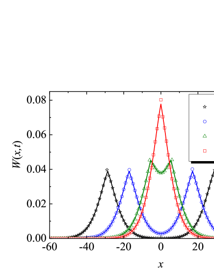
Figure 6: Lagrangian propagator at times $t=10^{4}$ for $v=10^{-2}$, $1.25\times 10^{-2}$, $1.5\times 10^{-2}$, and $v=x_{0}/T(10^{4})\approx 1.62\times 10^{-2}$. Solid lines: Propagator obtained from the numerical integration of the fractional diffusion equation. We used a fractional Crank-Nicolson algorithm with $\Delta t=0.1$ and $\Delta x=0.2$. The symbols depict simulations results ($10^{6}$ runs). The remaining parameters are: $x_{0}=75$, $\gamma=1/2$, $t_{0}=10^{3}$, $\alpha=1/2$, and $K_{\alpha}=1/2$.

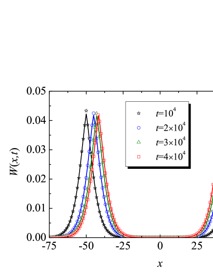
Figure 7: Lagrangian propagator obtained from the numerical integration of the fractional diffusion equation for $\alpha=1/2$, $K_{\alpha}=1/2$, $a(t)=(1+t/5000)^{2}$, $x_{0}=75$, and $v=7.5\times 10^{-3}$. We used a fractional Crank-Nicolson algorithm with $\Delta t=0.1$ and $\Delta x=0.2$. The symbols depict simulations results ($10^{6}$ runs).

4.2 Lévy flights

To conclude our study about pulse mixing, let us now focus on the specific case of Lévy flights corresponding to the parameter choice $\alpha=1$ and $0<\mu<2$. The solution for a two-pulse initial condition can be easily inferred from the one-particle propagator (50) for the zero-field case via the relation (99). The explicit form of the solution is

$$W(x,t)=\frac{1}{2}\left[\mathsf{L}_{\mu}\left(x+x_{0}-vT(t);[\sigma_{L}(t)]^{\mu}\right)+\mathsf{L}_{\mu}\left(x-x_{0}+vT(t);[\sigma_{L}(t)]^{\mu}\right)\right],$$ (105)

with $[\sigma_{L}(t)]^{\mu}=K_{1}^{\mu}\int_{0}^{t}a^{-\mu}(u)du$.

Let us once again consider the case of the power-law scale factor $a(t)=(1+t/t_{0})^{\gamma}$. As it turns out the asymptotic long-time behaviour of the typical width depends on whether $1/\mu$ is larger, equal, or smaller than $\gamma$. Table 2 summarises the typical subcases that result from the long-time behaviour of $T(t)$ and $w_{\mu}(t)$ for different values of $\gamma$ and $\mu$.

	$\gamma<\min\{1/\mu,1\}$	$1/\mu=\gamma<1$	$1/\mu<\gamma<1$	$\gamma=1<1/\mu$	$1/\mu=\gamma=1$	$1/\mu<\gamma=1$
$T$	$t^{1-\gamma}$	$t^{1-\gamma}$	$t^{1-\gamma}$	$\ln t$	$\ln t$	$\ln t$
$w_{\mu}$	$t^{1/\mu-\gamma}$	$(\ln t)^{1/\mu}$	$\mathrm{const.}$	$t^{1/\mu-\gamma}$	$(\ln t)^{1/\mu}$	$\mathrm{const.}$

	$1<\gamma<1/\mu$	$1<\gamma=1/\mu$	$\gamma>\max\{1,1/\mu\}$
$T$	$\mathrm{const.}$	$\mathrm{const.}$	$\mathrm{const.}$
$w_{\mu}$	$t^{1/\mu-\gamma}$	$(\ln t)^{1/\mu}$	$\mathrm{const.}$

Table 2: Asymptotic long-time behaviour of $T(t)$ and $w_{\mu}$ in the case of a power-law expansion with exponent $\gamma$.

Within the permitted range $0<\mu<2$ it is convenient to distinguish two subclasses of Lévy flights with different qualitative behaviour, i.e., flights with $\mu\geq 1$, and flights with $\mu<1$. For the first subclass the qualitative behaviour is similar to that of a Brownian process and is essentially obtained by performing the replacement $1/2\to 1/\mu$. Thus, for $v\neq 0$ the mixing of both pulses can be avoided for arbitrarily long times by choosing $\gamma>1$. However, when $v=0$ one must only have $\gamma>1/\mu$ in order to prevent mixing. The reason is that the respective pulse widths grow as $t^{1/\mu}$, which is not fast enough to ensure significant diffusive mixing of both pulses when their separation distance increases as $t^{\gamma}$ (with $\gamma>1/\mu$) due to the domain growth.

In contrast, for Lévy flights with $\mu<1$, the dominant contribution to mixing in the long time limit will stem from Lévy diffusion rather than from the biasing fields. Note that such a regime can never occur when the jump length PDF has a finite variance, i.e., in the normal-diffusive case or in the subdiffusive case.

The most clear-cut situation is found in the range $1<\gamma\leq 1/\mu$. In this regime, since $T_{\infty}<\infty$ the positions of both peaks tend to fixed limiting values. The advection velocity $v$ and the initial pulse separation $2x_{0}$ will determine whether or not such limiting values are attained before the two peaks meet. In either case diffusive spreading remains dominant with respect to the Hubble drift after a sufficiently long time and the pulse widths grow without bound. Consequently, at long times the mixing process proceeds via the widening of the respective pulses. Both pulses eventually merge into a single one, which still continues to widen. This is precisely what is seen in figure 8, which displays the evolution of the theoretical propagator for two Lévy pulses with characteristic exponent $\mu=3/4$ spreading on a domain whose growth is controlled by a power-law factor with $\gamma=5/4$ and $t_{0}=10^{3}$. The figure also shows simulations results that are in excellent agreement with the theoretical expression (105).

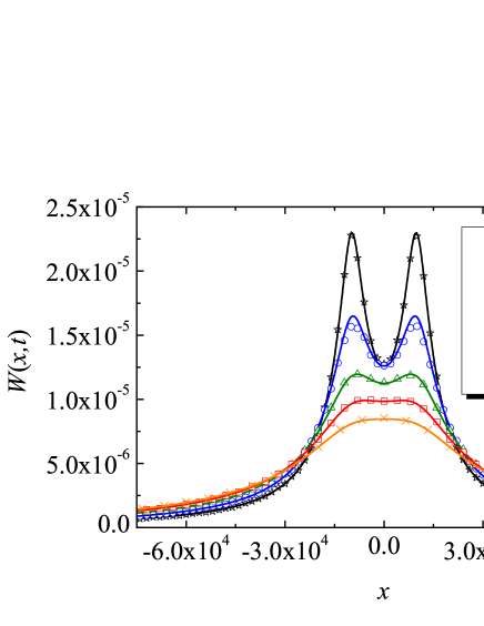
Figure 8: Lagrangian propagator at times $t=5\times 10^{3}$, $10^{4}$, $2.5\times 10^{4}$, $5\times 10^{4}$, and $10^{5}$ for two Lévy pulses with $\mu=3/4$, $K_{1}^{\mu}=1/2$, $x_{0}=10^{4}$, and $v=1/10$ for a domain growth rate given by the scale factor $a(t)=(1+t/10^{3})^{5/4}$. Solid lines represent the theoretical solution obtained from equation (105). Symbols depict simulations results ($10^{6}$ runs).

Finally, let us discuss the behaviour when $1<1/\mu<\gamma$. Here the diffusive spreading remains the main mixing mechanism over a transient period. However, the Hubble drift eventually becomes dominant, and consequently $W(x,t)$ tends to a stationary (frozen) profile in the long-time limit. Depending on the characteristic parameters ($\gamma$, $t_{0}$, $K_{1}^{\mu}$, $x_{0}$, and $v$) the distribution $W(x,t)$ will be single- or double-peaked at given time.

5 Summary and outlook

We investigated several aspects of an anomalous diffusion processes described by a separable CTRW evolving on a uniformly growing one-dimensional domain. First we studied the behaviour of the first moments in the symmetric case, with special focus on the rich phenomenology of the kurtosis. One of the most remarkable features is that this quantity becomes time dependent in the subdiffusive case. As a result of this, an initially non-Gaussian subdiffusive pulse was shown to exhibit a Gaussian-like long-time behaviour for a suitable parameter choice.

We subsequently considered the effect of a velocity field on this CTRW dynamics. We derived the corresponding FDAE (76), which generalises a previous result valid for the special case $\mu=2$ on a static domain[85]. Indeed, since our bifractional equation holds also for $\mu<2$, it includes Lévy flights as a particular case. The mathematical form of the FDAE is rather peculiar and not intuitive even in the case of a static domain, given the very straightforward Galilean transformation (58) between the walker’s PDF in the lab frame $\mathcal{S}_{L}$ and its counterpart in the comoving frame $\mathcal{S}_{0}$.

Taking the above results as a starting point we studied the mixing behaviour of a pair of diffusive pulses in a one-dimensional domain whose time evolution is governed by a power-law scale factor. We focused on the case where the pulses are drifting with velocities $v$ and $-v$ as they spread, the spreading of each pulse being characterised by their respective half-widths. In this scenario a sufficiently fast domain growth was found to largely prevent mixing between a pair of normal diffusive walkers or between a pair of subdiffusive walkers. However, a sufficiently large value of $v$ is able to restore mixing. In the superdiffusive case, the behaviour is more complex. For $\mu\geq 1$ and a sufficiently large initial separation of the pulses mixing is essentially controlled by the relative velocity introduced by the fields, as is the case for normal diffusive or for subdiffusive walkers. In contrast, when $\mu<1$, diffusional mixing dominates over the deterministic mixing induced by the velocity fields.

The present work may be extended in several directions. One such direction should consider the mixing behaviour of pulses for time dependent velocity fields $v=v(t)$. Another interesting generalisation concerns the case of non-separable CTRWs, e.g., Lévy walks. Finally, one could explore the effect of nonuniform domain growth [62] introducing a spatial dependence in the scale factor.

References

References

- [1] E. W. Montroll and G. H. Weiss, Random Walks on Lattices. III. Calculation of First-Passage Times with Application to Exciton Trapping on Photosynthetic Units, J. Math. Phys. 10, 753 (1969).
- [2] H. Scher and E. W. Montroll, Anomalous transit-time dispersion in amorphous solids, Phys. Rev. B 12, 2455 (1975).
- [3] H. Scher and M. Lax, Stochastic Transport in a Disordered Solid. I. Theory, Phys. Rev. B 7, 4491 (1973).
- [4] H. Krüsemann, R. Schwarzl, and R. Metzler, Ageing Scher-Montroll transport, Transp. Porous Media 115, 327 (2016).
- [5] A. V. Barzykin and M. Tachiya, Luminiscence Quenching in Micellar Clusters as a Random Walk Problem, Phys. Rev. Lett. 73, 3479 (1994).
- [6] G. Hornung, B. Berkowitz, and N. Barkai, Morphogen gradient formation in a complex environment: An anomalous diffusion model, Phys. Rev. E 72, 041916 (2005).
- [7] S. B. Yuste, E. Abad, and K. Lindenberg, Reaction-subdiffusion model of morphogen gradient formation, Phys. Rev. E 82, 061123 (2010).
- [8] P. Tan, Y. Liang, Q. Xu, E. Mamontov, J. Li, X. Xing, and L. Hong, Gradual crossover from subdiffusion to normal diffusion: a many-body effect in protein surface water, Phys. Rev. Lett. 120, 248101 (2018).
- [9] X. Hu, L. Hong, M. D. Smith, T. Neusius, X. Cheng, and J. C. Smith, The Dynamics of Single Protein Molecules is Non-Equilibrium and Self-Similar over Thirteen Decades in Time, Nature Phys. 12, 171 (2015).
- [10] A. V. Weigel, B. Simon, M. M. Tamkun, and D. Krapf, Ergodic and Nonergodic Processes Coexist in the Plasma Membrane as Observed by Single-Molecule Tracking, Proc. Natl. Acad. Sci. U.S.A. 108, 6438 (2011).
- [11] S. M. A. Tabei, S. Burov, H. Y. Kim, A. Kuznetsov, T. Huynh, J. Jureller, L. H. Philipson, A. R. Dinner, and N. F. Scherer, Intracellular Transport of Insulin Granules is a Subordinated Random Walk, Proc. Natl. Acad. Sci. U.S.A. 110, 4911 (2013).
- [12] J.-H. Jeon, V. Tejedor, S. Burov, E. Barkai, C. Selhuber-Unkel, K. Berg-Sørensen, L. Oddershede, and R. Metzler, In Vivo Anomalous Diffusion and Weak Ergodicity Breaking of Lipid Granules, Phys. Rev. Lett. 106, 048103 (2011).
- [13] K. Chen, B. Wang, and S. Granick, Memoryless self-reinforcing directionality in endosomal active transport within living cells, Nature Mat. 14, 589 (2015).
- [14] M. S. Song, H. C. Moon, J.-H. Jeon, and H. Y Park, Neuronal messenger ribonucleoprotein transport follows an aging Lévy walk, Nature Comm. 9, 344 (2018).
- [15] Y. Edery, A. Guadagnini, H. Scher, and B. Berkowitz, Origins of anomalous transport in heterogeneous media: Structural and dynamic controls, Wat. Resour. Res. 50, 1490 (2014).
- [16] H. Scher, G. Margolin, R. Metzler, J. Klafter, and B. Berkowitz, The dynamical foundation of fractal stream chemistry: The origin of extremely long retention times, Geophys. Res. Lett. 29, 1061 (2002).
- [17] E. Scalas, R. Gorenflo, and F. Mainardi, Fractional calculus and continuous time finance, Physica A 284, 376 (2000).
- [18] J. Masoliver, M. Montero, J. Perelló, and G. H. Weiss, The continuous time random walk formalism in financial markets, J. Econ. Behav. Organ. 61, 577 (2006).
- [19] H. Scher, M. F. Shlesinger, and J. T. Bendler, Time-scale invariance in transport and relaxation, Phys. Today 44, 26 (1991).
- [20] J. Klafter, M. F. Shlesinger, and G. Zumofen, Beyond Brownian motion, Phys. Today 49, 33 (1996).
- [21] M. F. Shlesinger, G. M. Zaslavsky, and J. Klafter, Strange kinetics, Nature 363, 31 (1993).
- [22] J.-P. Bouchaud and A. Georges, Anomalous diffusion in disordered media - statistical mechanisms, models and physical applications, Phys. Rep. 195, 127 (1990).
- [23] R. Metzler and J. Klafter, The random walk’s guide to anomalous diffusion: a fractional dynamics approach, Phys. Rep. 339, 1 (2000).
- [24] R. Metzler and J. Klafter, The restaurant at the end of the random walk: recent developments in the description of anomalous transport by fractional dynamics, J. Phys. A 37, R161 (2004).
- [25] I. M. Sokolov, Models of anomalous diffusion in crowded environments, Soft Matter 8, 9043 (2012).
- [26] R. Metzler, J.-H. Jeon, A. G. Cherstvy, and E. Barkai, Anomalous diffusion models and their properties: non-stationarity, non-ergodicity, and ageing at the centenary of single particle tracking, Phys. Chem. Chem. Phys. 16, 24128 (2014).
- [27] E. Barkai, Y. Garini, and R. Metzler, Strange Kinetics of Single Molecules in Living Cells, Phys. Today 65, 29 (2012).
- [28] D. Krapf and R. Metzler, Strange interfacial molecular dynamics, Phys. Today 72, 48 (2019).
- [29] B. D. Hughes, Random walks and random environments, vol. 1 (Oxford University Press, Oxford UK, 1990).
- [30] J.-P. Bouchaud, Weak ergodicity breaking and aging in disordered systems, J. Phys. (Paris) I 2, 1705 (1992).
- [31] G. Bel and E. Barkai, Weak Ergodicity Breaking in the Continuous-Time Random Walk, Phys. Rev. Lett. 94, 240602 (2005).
- [32] A. Rebenshtok and E. Barkai, Distribution of Time-Averaged Observables for Weak Ergodicity Breaking, Phys. Rev. Lett. 99, 210601 (2007).
- [33] M. A. Lomholt, I. M. Zaid, and R. Metzler, Subdiffusion and Weak Ergodicity Breaking in the Presence of a Reactive Boundary, Phys. Rev. Lett. 98, 200603 (2007).
- [34] S. Burov, R. Metzler, and E. Barkai, Aging and non-ergodicity beyond the Khinchin theorem, Proc. Natl. Acad. Sci. U.S.A. 107, 13228 (2010).
- [35] C. Monthus and J.-P. Bouchaud, Models of traps and glass phenomenology, J. Phys. A 29, 3847 (1996).
- [36] E. Barkai, Aging in Subdiffusion Generated by a Deterministic Dynamical System, Phys. Rev. Lett. 90, 104101 (2003).
- [37] J. H. P. Schulz, E. Barkai, and R. Metzler, Aging Effects and Population Splitting in Single-Particle Trajectory Averages, Phys. Rev. Lett. 110, 020602 (2013).
- [38] J. H. P. Schulz, E. Barkai, and R. Metzler, Aging Renewal Theory and Application to Random Walks, Phys. Rev. X 4, 011028 (2014).
- [39] C. Manzo, J. A. Torreno-Pina, P. Massignan, G. J. Lapeyre, Jr., M. Lewenstein, and M. F. Garcia Parajo, Weak Ergodicity Breaking of Receptor Motion in Living Cells Stemming from Random Diffusivity, Phys. Rev. X 5, 011021 (2015).
- [40] J. Klafter and R. Silbey, Derivation of the Continuous-Time Random-Walk Equation, Phys. Rev. Lett. 44, 55 (1980).
- [41] A. Compte, Stochastic foundations of fractional dynamics, Phys. Rev. E 53, 4191 (1996).
- [42] R. Metzler, E. Barkai, and J. Klafter, Anomalous diffusion and relaxation close to thermal equilibrium: A fractional Fokker-Planck equation approach, Phys. Rev. Lett. 82, 3563 (1999).
- [43] R. Metzler, E. Barkai, and J. Klafter, Deriving fractional Fokker-Planck equations from a generalised master equation, Europhys. Lett. 46, 431 (1999).
- [44] R. Metzler and J. Klafter, Boundary value problems for fractional diffusion equations, Physica A 278, 107 (2000).
- [45] E. Abad, S. B. Yuste, and K. Lindenberg, Reaction-subdiffusion and reaction-superdiffusion equations for evanescent particles performing continuous-time random walks, Phys. Rev. E 81, 031115 (2010).
- [46] S. B. Yuste, E. Abad, and K. Lindenberg, Exploration and Trapping of Mortal Random Walkers, Phys. Rev. Lett. 110, 220603 (2013).
- [47] E. Abad, S. B. Yuste, and K. Lindenberg, Evanescent continuous time random walks, Phys. Rev. E 88, 062110 (2013).
- [48] J. Klafter, S.-C. Lim, and R. Metzler, Editors, Fractional Dynamics in Physics (World Scientific, Singapore, 2011).
- [49] B. I. Henry and S. L. Wearne, Fractional reaction-diffusion, Physica A 276, 448 (2000).
- [50] I. M. Sokolov, M. G. W. Schmidt, and F. Sagués, Reaction-subdiffusion equations, Phys. Rev. E 73, 031102 (2006).
- [51] B. I. Henry, T. A. M. Langlands, and S. L. Wearne, Anomalous diffusion with linear reaction dynamics: From continuous time random walks to fractional reaction-diffusion equations, Phys. Rev. E 74, 031116 (2006).
- [52] A. Yadav and W. Horsthemke, Kinetic equations for reaction-subdiffusion systems: Derivation and stability analysis, Phys. Rev. E 74, 066118 (2006).
- [53] K. Seki, A. I. Shushin, M. Wojcik, and M. Tachiya, Specific features of the kinetics of fractional-diffusion assisted geminate reactions, J. Phys. Condens. Matter, 19, 065117 (2007).
- [54] S. Fedotov and A. Iomin, Probabilistic approach to a proliferation and migration dichotomy in tumor cell invasion, Phys. Rev. E 77, 031911 (2008).
- [55] A. Yadav, S. M. Milu, and W. Horsthemke, Turing instability in reaction-subdiffusion systems, Phys. Rev. E 78, 026116 (2008).
- [56] V. Gafiychuk, B. Datsko, and V. Meleshko, Mathematical modeling of time fractional reaction-diffusion systems, J. Comput. Appl. Math. 220, 215 (2008).
- [57] D. Froemberg and I. M. Sokolov, Stationary fronts in an A + B –> 0 reaction under subdiffusion, Phys. Rev. Lett. 100, 108304 (2008).
- [58] V. Méndez, S. Fedotov, and W. Horsthemke, Reaction-Transport Systems: Mesoscopic Foundations, Fronts, and Spatial Instabilities (Springer-Verlag, 2010).
- [59] F. Le Vot, E. Abad, and S. B. Yuste, Continuous-time random-walk model for anomalous diffusion in expanding media, Phys. Rev. E 96, 032117 (2017).
- [60] C. N. Angstmann, B. I. Henry, and A. V. McGann, Generalized fractional diffusion equations for subdiffusion in arbitrarily growing domains, Phys. Rev. E 96, 042153 (2017).
- [61] F. Le Vot and S. B. Yuste, Continuous-time random walks and Fokker-Planck equation in expanding media, Phys. Rev. E. 98, 042117 (2018).
- [62] E. Abad, C. N. Angstmann, B. I. Henry, A. V. McGann, F. Le Vot, and S. B. Yuste, Reaction-diffusion and reaction-subdiffusion equations on arbitrarily evolving domains, arXiv:2002.06011.
- [63] S.B. Yuste, E. Abad, and C. Escudero, Diffusion in an expanding medium: Fokker-Planck equation, Green’s function, and first-passage properties, Phys. Rev. E 94, 032118 (2016).
- [64] F. Le Vot, C. Escudero, E. Abad, and S. B. Yuste, Encounter-controlled coalescence and annihilation on a one-dimensional growing domain, Phys. Rev. E 98 032137 (2018).
- [65] C. Escudero, S. B. Yuste, E. Abad, and F. Le Vot, Reaction-diffusion kinetics in growing domains, Handbook of Statistics 39, 131 (2018).
- [66] E. Abad, C. Escudero, F. Le Vot, and S. B. Yuste, First-Passage Processes and Encounter-Controlled Reactions in Growing Domains, in Chemical Kinetics: Beyond the Textbook, edited by K. Lindenberg, R. Metzler, and G. Oshanin, pp. 409-433 (World Scientific, Singapore, 2019).
- [67] B. Alberts, A. Johnson, J. Lewis, D. Morgan, M. Raff, K. Roberts, and P. Walter, Molecular biology of the cell, 6th ed. (Garland Science, New York, 2015).
- [68] C. Wilson et al, Quantitative and Qualitative Assessment Methods for Biofilm Growth: A Mini-review, Res. Rev. J. Eng. Technol. 6, 1 (2017).
- [69] H.-C. Flemming et al, Biofilms: an emergent form of bacterial life, Nature Rev. Microbiol. 14, 563 (2016).
- [70] D. Ambrosi, M. Ben Amar, C. J. Cyron, A. DeSimone, A. Goriely, J. D. Humphrey and E. Kuhl, Growth and remodelling of living tissues: perspectives, challenges and opportunities, J. R. Soc. Interface 16, 20190233 (2019).
- [71] S. C. Cowin, Tissue growth and remodeling, Annu. Rev. Biomed. Eng. 6, 77 (2004).
- [72] J. W. Szostak, D. P. Bartel, and P. L. Luisi, Synthesizing life, Nature 409, 387 (2001).
- [73] C. Xu, S. Hu, and X. Chen, Artificial cells: from basic science to applications, Mater. Today 19, 516 (2016).
- [74] B. L.-S. Mui, P. R. Cullis, E. Evans, and T. D. Madden, Osmotic properties of large unilamellar vesicles prepared by extrusion, Biophys. J. 64, 443 (1993).
- [75] O. Carrier, N. Shahidzadeh-Bonn, R. Zargar, M. Aytouna, M. Habibi, J. Eggers, and D. Bonn, Evaporation of water: evaporation rate and collective effects, J. Fluid Mech. 798, 774 (2016).
- [76] Q. Yang and B. R. Scanion, How much water can be captured from flood flows to store in depleted aquifers for mitigating floods and droughts? A case study from Texas, US, Environ. Res. Lett. 14, 054011 (2019).
- [77] G. Zhang, G. Feng, X. Li, C. Xie, and X. Pi, Flood Effect on Groundwater Recharge on a Typical Silt Loam Soil, Water 9, 523 (2017).
- [78] C. J. All gre and D. L. Turcotte, Implications of a two-component marble-cake mantle, Nature 323, 123 (1986).
- [79] L. H. Kellogg and D. L. Turcotte, Homogenization of the mantle by convective mixing and diffusion, Earth Planet. Sci. Lett. 81, 371 (1987).
- [80] V. Berezinsky and A. Z. Gazizov, Diffusion of Cosmic Rays in the Expanding Universe. II. Energy Spectra of Ultra-High Energy Cosmic Rays, Astrophys. J. 669, 684 (2007).
- [81] R. A. Batista and G. Sigl, Diffusion of cosmic rays at EeV energies in inhomogeneous extragalactic magnetic fields, J. Cosmol. Astropart. Phys. 1, 031 (2014).
- [82] F. Le Vot, E. Abad, and S. B. Yuste, Standard and fractional Ornstein-Uhlenbeck process on a growing domain, Phys. Rev. E 100, 012142 (2019).
- [83] M. S. Song, H. C. Moon, J.-H. Jeon, and H. Y. Park, Neuronal messenger ribonucleoprotein transport follows an aging Lévy walk, Nature Comm. 9, 344 (2018).
- [84] Y. Chen, X. Wang, and W. Deng, Subdiffusion in an external force field, Phys. Rev. E 99, 042125 (2019).
- [85] A. Cairoli, R. Klages, and A. Baule, Weak Galilean invariance as a selection principle for coarse-grained diffusive models, Proc. Natl. Acad. Sci. U.S.A. 115, 5714 (2018).
- [86] I. Podlubny, Fractional Differential Equations: An Introduction to Fractional Derivatives, Fractional Differential Equations, to Methods of Their Solution and Some of Their Applications (Academic Press, San Diego, 1999).
- [87] A. M. Mathai, R. K. Saxena, and H. J. Haubold, The H-Function: Theory and Applications (Springer, Berlin, 2009).
- [88] M. Abramowitz and I. Stegun, Handbook of Mathematical Functions (Dover publications, New York, 1972).
- [89] S. B. Yuste, Weighted average finite difference methods for fractional diffusion equations, J. Comput. Phys. 216, 264 (2006).
- [90] I. M. Sokolov and R. Metzler, Towards deterministic equations for Lévy walks: The fractional material derivative, Phys. Rev. E 98, 042117 (2003).
- [91] V. V. Uchaikin, R. T. Sibatov, and A. N. Byzykchi, Cosmic rays propagation along solar magnetic field lines: a fractional approach, Commun. Appl. Ind. Math. 6, e-479 (2014).
- [92] R. Metzler, J. Klafter, and I. M. Sokolov, Anomalous transport in external fields: Continuous time random walks and fractional diffusion equations extended, Phys. Rev. E 58, 1621 (1998).
- [93] K. S. Fa, Continuous time random walk: Galilei invariance and relation for the nth moment, J. Phys. A: Math. Theor. 44, 035004 (2011).
- [94] B. Ryden, Introduction to Cosmology (Addison-Wesley, Reading, 2003).
- [95] M. v. Smoluchowski, Three presentations on diffusion, molecular movement according to Brown and coagulation of colloid particles, Physikal. Zeitschr. 17, 557 (1916).
- [96] M. Ptashne, A Genetic Switch, Phage Lambda Revisited (Cold Spring Harbor Laboratory Press, Cold Spring Harbor, 2004).
- [97] O. Pulkkinen and R. Metzler, Distance matters: the impact of gene proximity in bacterial gene regulation, Phys. Rev. Lett. 110, 198101 (2013).
- [98] A. Godec and R. Metzler, Universal proximity effect in target search kinetics in the few encounter limit, Phys. Rev. X 6, 041037 (2016).
- [99] Y. Elani, R. V. Law, and O. Ces, Protein synthesis in artificial cells: using compartmentalisation for spatial organisation in vesicle bioreactors, Phys. Chem. Chem. Phys. 17, 15534 (2015).