Three Modern Roles for Logic in AI

Abstract.

We consider three modern roles for logic in artificial intelligence, which are based on the theory of tractable Boolean circuits: (1) logic as a basis for computation, (2) logic for learning from a combination of data and knowledge, and (3) logic for reasoning about the behavior of machine learning systems.

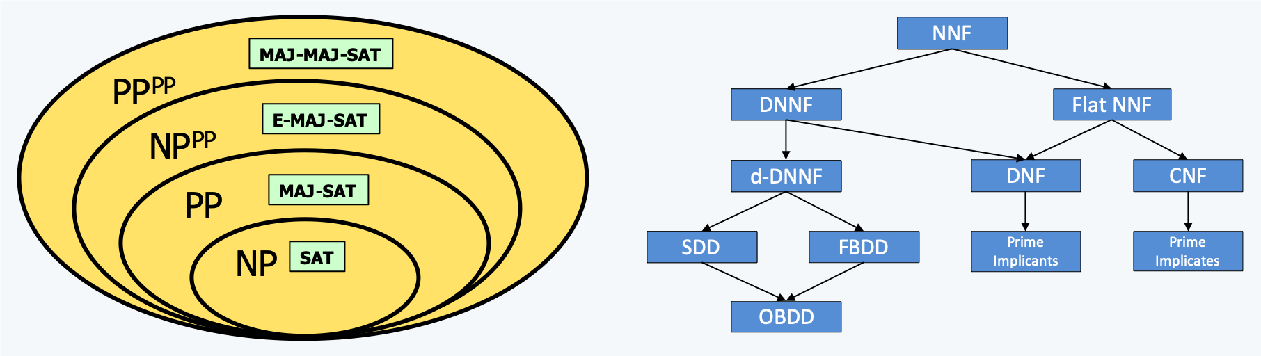
Figure 1. Tractable Boolean circuits as a basis for computation.

Tractable Boolean circuits as a basis for computation.

1. Introduction

Logic has played a fundamental role in artificial intelligence since the field was incepted (McCarthy, 1959). This role has been mostly in the area of knowledge representation and reasoning, where logic is used to represent categorical knowledge and then draw conclusions based on deduction and other more advanced forms of reasoning. Starting with (Nilsson, 1986), logic also formed the basis for drawing conclusions from a mixture of categorial and probabilistic knowledge.

In this paper, we review three modern roles for propositional logic in artificial intelligence, which are based on the theory of tractable Boolean circuits. This theory, which matured considerably during the last two decades, is based on Boolean circuits in Negation Normal Form (NNF) form. NNF circuits are not tractable, but they become tractable once we impose certain properties on them (Darwiche and Marquis, 2002). Over the last two decades, this class of circuits has been studied systematically across three dimensions. The first dimension concerns a synthesis of NNF circuits that have varying degrees of tractability (the polytime queries they support). The second dimension concerns the relative succinctness of different classes of tractable NNF circuits (the optimal size circuits can attain). The third dimension concerns the development of algorithms for compiling Boolean formula into tractable NNF circuits.

The first modern role for logic we consider is in using tractable circuits as a basis for computation, where we show how problems in the complexity classes $\mathsf{NP}$, $\mathsf{PP}$, $\mathsf{NP}^{\mathsf{PP}}$ and $\mathsf{PP}^{\mathsf{PP}}$ can be solved by compiling Boolean formula into corresponding tractable circuits. These are rich complexity classes, which include some commonly utilized problems from probabilistic reasoning and machine learning. We discuss this first role in two steps. In Section 2, we discuss the prototypical problems that are complete for these complexity classes, which are all problems on Boolean formula. We also discuss problems from probabilistic reasoning which are complete for these classes and their reduction to prototypical problems. In Section 3, we introduce the theory of tractable circuits with exposure to circuit types that can be used to efficiently solve problems in these complexity classes (if compiled successfully).

The second role for logic we shall consider is in learning from a combination of data and symbolic knowledge. We show again that this task can be reduced to a process of compiling, then reasoning with, tractable circuits. This is discussed in Section 4, where we also introduce and employ a class of tractable probabilistic circuits that are based on tractable Boolean circuits.

The third role for logic that we consider is in meta-reasoning, where we employ it to reason about the behavior of machine learning systems. In this role, some common machine learning classifiers are compiled intro tractable circuits that have the same input-output behavior. Queries pertaining to the explainability and robustness of decisions can then be answered efficiently, while also allowing one to formally prove global properties of the underlying machine learning classifiers. This role is discussed in Section 5.

The paper concludes in Section 6 with a perspective on research directions that can mostly benefit the roles we shall discuss, and a perspective on how recent developments in AI have triggered some transitions that remain widely unnoticed.

2. Logic For Computation

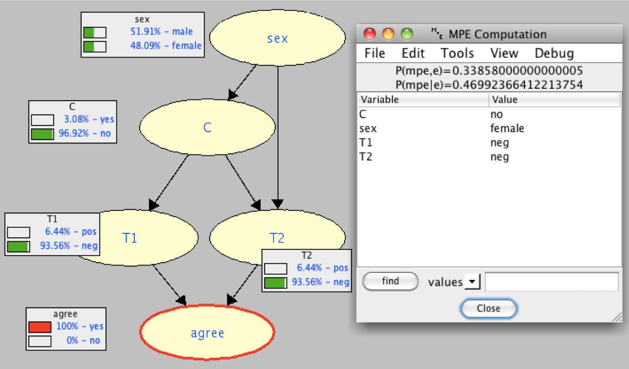
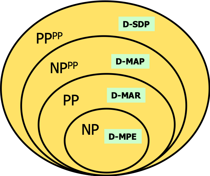
Figure 2. Left: A Bayesian network with an illustration of the MPE query. The network concerns a medical condition c and two tests t1 and t2 that can be used to detect the condition. The variable agree indicates whether the two test results are in agreement. Right: Decision problems on Bayesian networks that are complete for the classes $\mathsf{NP}$, $\mathsf{PP}$, $\mathsf{NP}^{\mathsf{PP}}$ and $\mathsf{PP}^{\mathsf{PP}}$.

Complexity of Bayesian network queries.

The first role we shall consider for logic is that of systematically solving problems in the complexity classes $\mathsf{NP}$, $\mathsf{PP}$, $\mathsf{NP}^{\mathsf{PP}}$ and $\mathsf{PP}^{\mathsf{PP}}$, which are related in the following way:

$$\mathsf{NP}\subseteq\mathsf{PP}\subseteq\mathsf{NP}^{\mathsf{PP}}\subseteq\mathsf{PP}^{\mathsf{PP}}.$$

The prototypical problems for these complexity classes all correspond to questions on Boolean formula. Moreover, these classes include problems that are commonly used in the areas of probabilistic reasoning and machine learning. While there is a long tradition of developing dedicated algorithms when tackling problems in these complexity classes, it is now common to solve such problems by reducing them to their Boolean counterparts, especially for problems with no tradition of dedicated algorithms.

Let us first consider four common problems from probabilistic reasoning and machine learning that are complete for the classes $\mathsf{NP}$, $\mathsf{PP}$, $\mathsf{NP}^{\mathsf{PP}}$ and $\mathsf{PP}^{\mathsf{PP}}$. These problems can all be stated on probability distributions specified using Bayesian networks (Darwiche, 2009; Pearl, 1988; Koller and Friedman, 2009; Murphy, 2012). These networks are directed acyclic graphs with nodes representing (discrete) variables. Figure 2 depicts a Bayesian network with five variables sex, c, t1, t2 and agree. The structure of a Bayesian network encodes conditional independence relations among its variables. Each network variable is associated with a set of distributions that are conditioned on the states of its parents (not shown in Figure 2). These conditional probabilities and the conditional independences encoded by the network structure are satisfied by exactly one probability distribution over the network variables. There are four question on this distribution whose decision versions are complete for the complexity classes $\mathsf{NP}$, $\mathsf{PP}$, $\mathsf{NP}^{\mathsf{PP}}$ and $\mathsf{PP}^{\mathsf{PP}}$. Before we discuss these problems, we settle some notation first.

Upper case letters (e.g., $X$) will denote variables and lower case letters (e.g., $x$) will denote their instantiations. That is, $x$ is a literal specifying a value for variable $X$. Bold upper case letters (e.g., ${\bf X}$) will denote sets of variables and bold lower case letters (e.g., ${\bf x}$) will denote their instantiations. We liberally treat an instantiation of a variable set as conjunction of its corresponding literals.

The four problems we shall consider on a Bayesian network with variables ${\bf X}$ and distribution ${\it Pr}({\bf X})$ are MPE, MAR, MAP and SDP. The MPE problem finds an instantiation ${\bf x}$ of the network variables that has a maximal probability ${\it Pr}({\bf x})$. This is depicted in Figure 2 which illustrates the result of an MPE computation. The decision version of this problem, D-MPE, asks whether there is a variable instantiation whose probability is greater than a given $k$. The decision problem D-MPE is complete for the class $\mathsf{NP}$ (Shimony, 1994).

We next have MAR which computes the probability of some value $x$ for a variable $X$. Figure 2 depicts these probabilities for each variable/value pair. The decision version, D-MAR, asks whether ${\it Pr}(x)$ is greater than a given $k$. D-MAR is complete for the class $\mathsf{PP}$ (Roth, 1996). MAR is perhaps the most commonly used query on Bayesian networks and similar probabilistic graphical models.

The next two problems are stated with respect to a subset of network variables ${\bf Y}\subseteq{\bf X}$. The problem MAP finds an instantiation ${\bf y}$ that has a maximal probability. For example, we may wish to find a most probable instantiation of variables sex and c in Figure 2. The decision version of this problem, D-MAP, asks whether there is an instantiation ${\bf y}$ whose probability is greater than a given $k$. D-MAP is complete for the class $\mathsf{NP}^{\mathsf{PP}}$ (Park and Darwiche, 2004).

Suppose now that we are making a decision based on whether ${\it Pr}(x)\geq T$ for some variable value $x$ and threshold $T$. The SDP problem finds the probability that this decision will stick after having observed the state of variables ${\bf Y}$. For example, we may want to operate on a patient if the probability of condition c in Figure 2 is greater than $90\%$ (the decision is currently negative). The SDP (same-decision probability) can be used to compute the probability that this decision will stick after having obtained the results of tests t1 and t2 (Darwiche and Choi, 2010). The SDP computes an expectation. Its decision version, D-SDP, asks whether this probability is greater than a given $k$ and is complete for the class $\mathsf{PP}^{\mathsf{PP}}$ (Choi et al., 2012). This query was used to assess the value of information with applications to reasoning about features in Bayesian network classifiers; see, e.g., (Chen et al., 2015; Choi et al., 2017a; Choi and den Broeck, 2018).

There is a tradition of solving the above problems using dedicated algorithms; see, e.g., the treatments in (Darwiche, 2009; Pearl, 1988; Koller and Friedman, 2009; Murphy, 2012). Today these problems are also being commonly solved using reductions to the prototypical problems of the corresponding complexity classes, which are defined over Boolean formula as mentioned earlier. This is particularly the case for the MAR problem and for distributions that are specified by representations that go beyond Bayesian networks; see, e.g., (Manhaeve et al., 2018; Latour et al., 2017; Dries et al., 2015). These reduction-based approaches are the state of the art on certain problems; for example, when the Bayesian network has an abundance of 0/1 probabilities or context-specific independence (Darwiche et al., 2008).

We next discuss the prototypical problems of complexity classes $\mathsf{NP}$, $\mathsf{PP}$, $\mathsf{NP}^{\mathsf{PP}}$ and $\mathsf{PP}^{\mathsf{PP}}$ before we illustrate in Section 2.2 the core technique used in reductions to these problems. We then follow in Section 3 by showing how these prototypical problems can be solved systematically by compiling Boolean formula into Boolean circuits with varying degrees of tractability.

2.1. Prototypical Problems

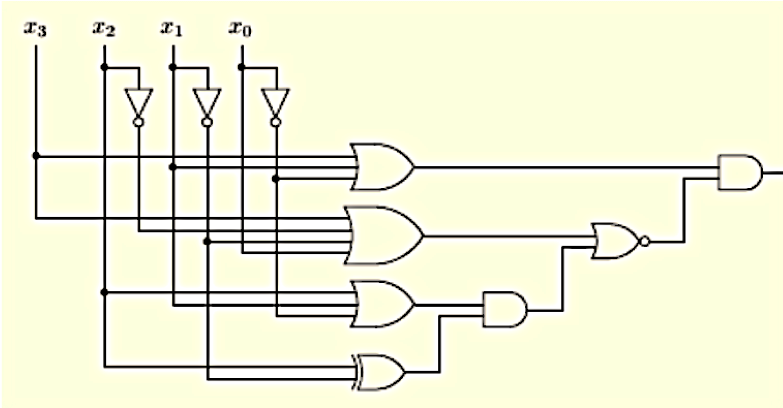
Figure 3. A Boolean circuit to illustrate the problems Sat, MajSat, E-MajSat and MajMajSat.

Sat, MajSat, E-MajSat, MajMajSat.

$\mathsf{NP}$ is the class of decision problems that can be solved by a non-deterministic polynomial-time Turing machine. $\mathsf{PP}$ is the class of decision problems that can be solved by a non-deterministic polynomial-time Turing machine, which has more accepting than rejecting paths. $\mathsf{NP}^{\mathsf{PP}}$ and $\mathsf{PP}^{\mathsf{PP}}$ are the corresponding classes assuming the corresponding Turing machine has access to a $\mathsf{PP}$ oracle.

The prototypical problems for these classes are relatively simple and are usually defined on Boolean formula in Conjunctive Normal Form (CNF). We will however illustrate them on Boolean circuits to make a better connection to the discussion in Section 3.

Consider a Boolean circuit $\Delta$ which has input variables ${\bf X}$ and let $\Delta({\bf x})$ be the output of this circuit given input ${\bf x}$; see Figure 3. The following decision problems are respectively complete and prototypical for the complexity classes $\mathsf{NP}$, $\mathsf{PP}$, $\mathsf{NP}^{\mathsf{PP}}$ and $\mathsf{PP}^{\mathsf{PP}}$.

—Sat asks if there is a circuit input ${\bf x}$ such that $\Delta({\bf x})=1$.

—MajSat asks if the majority of circuit inputs ${\bf x}$ are such that $\Delta({\bf x})=1$.

The next two problems require that we partition the circuit input variables ${\bf X}$ into two sets ${\bf Y}$ and ${\bf Z}$.

—E-MajSat asks if there is a circuit input ${\bf y}$ such that $\Delta({\bf y},{\bf z})=1$ for the majority of circuit inputs ${\bf z}$.

—MajMajSat asks if the majority of circuit inputs ${\bf y}$ are such that $\Delta({\bf y},{\bf z})=1$ for the majority of circuit inputs ${\bf z}$.

There are two functional versions of MajSat which have been receiving increased attention recently. The first is #Sat which asks for the number of circuit inputs ${\bf x}$ such that $\Delta({\bf x})=1$. Algorithms that solve this problem are known as model counters. The more general functional version of MajSat and the one typically used in practical reductions is called weighted model counting, WMC. In this variant, each circuit input $x$ for variable $X$ is given a weight $W(x)$. A circuit input ${\bf x}=x_{1},\ldots,x_{n}$ is then assigned the weight $W({\bf x})=W(x_{1})\ldots W(x_{n})$. Instead of counting the number of inputs ${\bf x}$ such that $\Delta({\bf x})=1$, weighted model counting adds up the weights of such inputs. That is, WMC computes $\sum_{\bf x}W({\bf x})$ for all circuit inputs ${\bf x}$ such that $\Delta({\bf x})=1$.

2.2. The Core Reduction

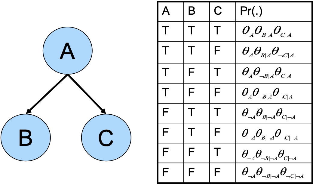
Figure 4. A Bayesian network and its distribution.

The distribution of a Bayesian network.

As mentioned earlier, the decision problems Sat, MajSat, E-MajSat and MajMajSat on Boolean formula are complete and prototypical for the complexity classes $\mathsf{NP}$, $\mathsf{PP}$, $\mathsf{NP}^{\mathsf{PP}}$ and $\mathsf{PP}^{\mathsf{PP}}.$ The decision problems D-MPE, D-MAR, D-MAP and D-SDP on Bayesian networks are also complete for these complexity classes, respectively. Practical reductions of the latter problems to the former ones have been developed over the last two decades; see (Darwiche, 2009, Chapter 11) for a detailed treatment. Reductions have also been proposed from the functional problem MAR to WMC, which are of most practical significance. We will next discuss the first such reduction (Darwiche, 2002) since it is relatively simple yet gives the essence of how one can reduce problems that appear in probabilistic reasoning and machine learning to problems on Boolean formula and circuits. In Section 3, we will further show how these problems (of numeric nature) can be competitively solved using purely symbolic manipulations.

Consider the Bayesian network in Figure 4, which has three binary variables $A$, $B$ and $C$. Variable $A$ has one distribution $(\theta_{A},\theta_{\neg A})$. Variable $B$ has two distributions, which are conditioned on the state of its parent $A$: $(\theta_{B|A},\theta_{\neg B|A})$ and $(\theta_{B|\neg A},\theta_{\neg B|\neg A})$. Variable $C$ also has two similar distributions: $(\theta_{C|A},\theta_{\neg C|A})$ and $(\theta_{C|\neg A},\theta_{\neg C|\neg A})$. We will refer to the probabilities $\theta$ as network parameters. The Bayesian network in Figure 4 has ten parameters.

This Bayesian network induces the distribution depicted in Figure 4, where the probability of each variable instantiation is simply the product of network parameters that are compatible with that instantiation; see (Darwiche, 2009, Chapter 3) for a discussion of the syntax and semantics of Bayesian networks. We will next show how one can efficiently construct a Boolean formula $\Delta$ from a Bayesian network, allowing one to compute marginal probabilities on the Bayesian network by performing weighted model counting on formula $\Delta$.

The main insight is to introduce a Boolean variable $P$ for each network parameter $\theta$, which is meant to capture the presence or absence of parameter $\theta$ given an instantiation of the network variables (i.e., a row of the table in Figure 4). For the network in Figure 4, this leads to introducing ten Boolean variables: $P_{A}$, $P_{\neg A}$, $P_{B|A},\ldots,P_{\neg C|\neg A}$. In the second row of Figure 4, which corresponds to variable instantiation $A,B,\neg C$, parameters $\theta_{A}$, $\theta_{B|A}$ and $\theta_{\neg C|A}$ are present and the other seven parameters are absent.

We can capture such presence/absence by adding one expression to the Boolean formula $\Delta$ for each network parameter. For example, the parameters associated with variable $A$ introduce the following expressions: $A\iff P_{A}$ and $\neg A\iff\neg P_{\neg A}$. Similarly, the parameters of variable $B$ introduce the expressions $A\wedge B\iff P_{B|A}$, $\>\>A\wedge\neg B\iff P_{\neg B|A}$, $\>\>\neg A\wedge B\iff P_{B|\neg A}$ and $\>\>\neg A\wedge\neg B\iff P_{\neg B|\neg A}$. The parameters of variable $C$ introduce similar expressions.

The resulting Boolean formula $\Delta$ will have exactly eight models, which correspond to the network instantiations. The following is one of these models which correspond to instantiation $A,B,\neg C$:

$$A\>\>B\>\>\neg C\>\>P_{A}\>\>P_{B|A}\>\>P_{\neg C|A}$$

(1) $$\neg P_{\neg A}\>\>\>\neg P_{\neg B|A}\neg P_{B|\neg A}\neg P_{\neg B|\neg A}\>\>\>\neg P_{C|A}\neg P_{C|\neg A}\neg P_{\neg C|\neg A}.$$

In this model, all parameters associated with instantiation $A,B,\neg C$ appear positively (present) while others appear negatively (absent).

The last step is to assign weights to the values of variables (literals). For network variables, all literals get a weight of $1$; for example, $W(A)=1$ and $W(\neg A)=1$. The negative literals of parameter variables also get a weight of $1$; for example, $W(\neg P_{A})=1$ and $W(\neg P_{\neg C|A})=1$. Finally, positive literals of network parameters get weights equal to these parameters; for example, $W(P_{A})=\theta_{A}$ and $W(P_{\neg C|A})=\theta_{\neg C|A}$. The weight of expression (1) is then $\theta_{A}\theta_{B|A}\theta_{\neg C|A}$, which is precisely the probability of network instantiation $A,B,\neg C$. We can now compute the probability of any Boolean expression $\alpha$ by simply computing the weighted model count of $\Delta\wedge\alpha$, which completes the reduction of MAR to WMC.

Another reduction was proposed in (Sang et al., 2005) which is suited towards Bayesian networks that have variables with large cardinalities. More refined reductions have also been proposed which can capture certain properties of network parameters such as 0/1 parameters and context-specific independence (can be critical for the efficient computation of weighted model counts on the resulting Boolean formula). A detailed treatment of reduction techniques and various practical tradeoffs can be found in (Chavira and Darwiche, 2008) and (Darwiche, 2009, Chapter 13).

3. Tractable Circuits

Figure 5. Negation Normal Form (NNF) circuit.

Negation Normal Form circuit (NNF circuit).

We now turn to a systematic approach for solving prototypical problems in the classes $\mathsf{NP}$, $\mathsf{PP}$, $\mathsf{NP}^{\mathsf{PP}}$ and $\mathsf{PP}^{\mathsf{PP}},$ which is based on compiling Boolean formula into tractable Boolean circuits. The circuits we shall compile into are in Negation Normal Form (NNF) as depicted in Figure 5. These circuits have three types of gates: and-gates, or-gates and inverters, except that inverters can only feed from the circuit variables. Any circuit with these types of gates can be converted to an NNF circuit while at most doubling its size.

NNF circuits are not tractable. However, by imposing certain properties on them we can attain different degrees of tractability. The results we shall review next are part of the literature on knowledge compilation, an area that has been under development for a few decades, see, e.g., (Selman and Kautz, 1996; Cadoli and Donini, 1997; Marquis, 1995), except that it took a different turn since (Darwiche and Marquis, 2002); see also (Darwiche, 2014). Earlier work on knowledge compilation focused on flat NNF circuits, which include subsets of Conjunctive Normal Form (CNF) and Disjunctive Normal Form (DNF) such as prime implicates, Horn clauses and prime implicants. Later, however, the focus shifted towards deep NNF circuits with no restriction on the number of circuit layers. A comprehensive treatment was initially given in (Darwiche and Marquis, 2002), in which some tractable NNF circuits were studied across the two dimensions of tractability and succinctness. As we increase the strength of properties imposed on NNF circuits, their tractability increases by allowing more queries to be performed in polytime. This, however, typically comes at the expense of succinctness as the size of circuits gets larger.

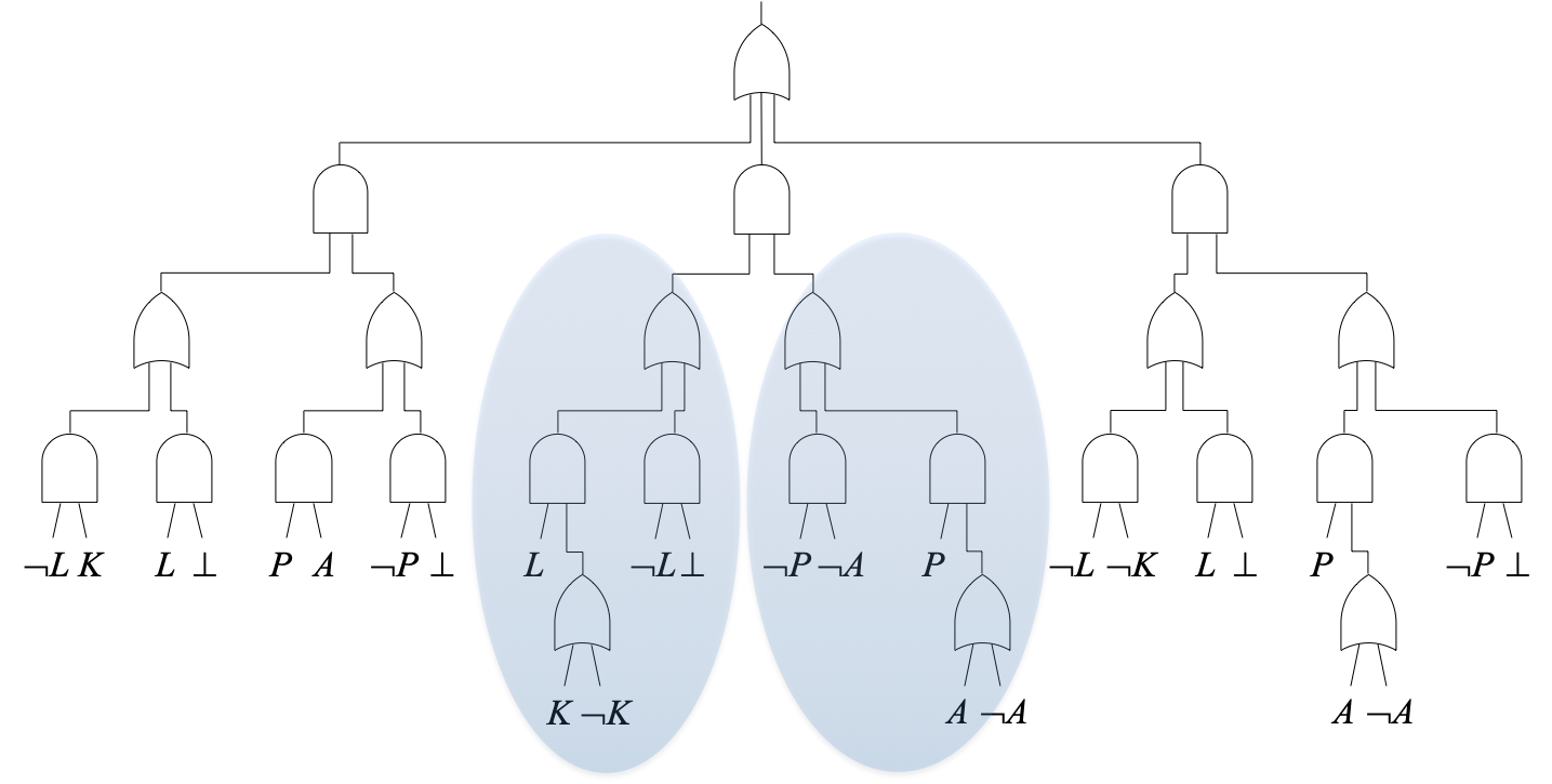
Figure 6. Illustrating the decomposability property of NNF circuits. The illustration does not tie shared inputs of the circuit for clarity of exposition.

Decomposable NNF circuits (DNNF circuits).

One of the simplest properties that turn NNF circuits into tractable ones is decomposability (Darwiche, 2001a). According to this property, subcircuits feeding into an and-gate cannot share circuit variables. Figure 6 illustrates this property by highlighting the two subcircuits (in blue) feeding into an and-gate. The subcircuit on the left feeds from circuit variables $K$ and $L$, while the one on the right feeds from circuit variables $A$ and $P$. NNF circuits that satisfy the decomposability property are known as Decomposable NNF (DNNF) circuits. The satisfiability of DNNF circuits can be decided in time linear in the circuit size (Darwiche, 2001a). Hence, enforcing decomposability is sufficient to unlock the complexity class $\mathsf{NP}.$

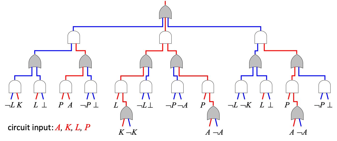
Figure 7. Illustrating the determinism property of NNF circuits. Red wires are high and blue ones are low.

Deterministic, decomposable NNF circuits (d-DNNF circuits).

The next property we consider is determinism (Darwiche, 2001b), which applies to or-gates in an NNF circuit. According to this property, at most one input for an or-gate must be high under any circuit input. Figure 7 illustrates this property when all circuit variables $A,K,L,P$ are high. Examining the or-gates in this circuit, under this circuit input, one sees that each or-gate has either one high input or no high inputs. This property corresponds to mutual exclusiveness when the or-gate is viewed as a disjunction of its inputs. MajSat can be decided in polytime on NNF circuits that are both decomposable and deterministic. These circuits are called d-DNNF circuits. If they are also smooth (Darwiche, 2003), a property that can be enforced in quadratic time, d-DNNF circuits allow one to perform weighted model counting (WMC) in linear time. The combination of decomposability and determinism therefore unlocks the complexity class $\mathsf{PP}$.

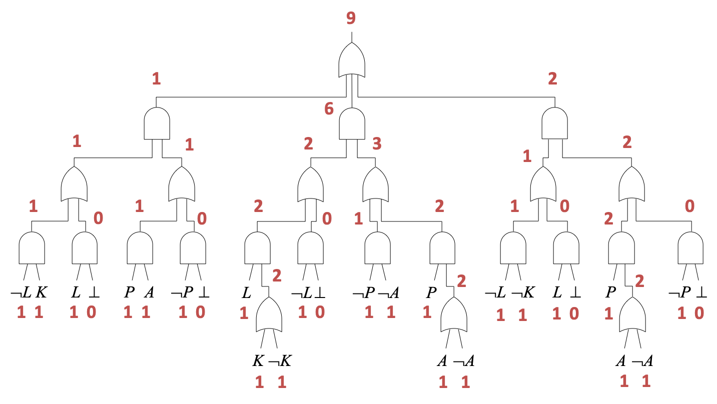
Figure 8. Model counting in linear time on d-DNNF circuits.

Model counting using d-DNNF circuits.

Smoothness requires that all subcircuits feeding into an or-gate mention the same circuit variables. For example, in Figure 7, three subcircuits feed into the top or-gate. Each of these subcircuits mentions the same set of circuit variables: $A,K,L,P$. Enforcing smoothness can introduce trivial gates into the circuit such as the bottom three or-gates in Figure 7 and can sometimes be done quite efficiently (Shih et al., 2019c). An example of model counting using a d-DNNF circuit is depicted in Figure 8. Every circuit literal, whether a positive literal such as $A$ or a negative literal such as $\neg A$, is assigned the value $1$. Constant inputs $\top$ and $\bot$ are assigned the values $1$ and $0$. We then propagate these numbers upwards, multiplying numbers assigned to the inputs of an and-gate and summing numbers assigned to the inputs of an or-gate. The number we obtain for the circuit output is the model count. In this example, the circuit has $9$ satisfying inputs out of $16$ possible ones. To perform weighted model counting, we simply assign a weight to a literal instead of the value $1$—model counting (#Sat) is a special case of weighted model counting (WMC) when the weight of each literal is $1$.

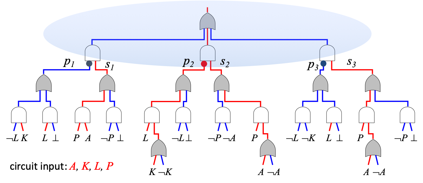
Figure 9. Illustrating the sentential decision property of NNF circuits. Red wires are high and blue ones are low.

Sentential Decision Diagrams (SDD circuits).

(a) vtree

(b) constrained $CE|ABD$

(c) right-linear

Figure 10. A constrained vtree for ${\bf X}|{\bf Y}$ is a vtree over variables ${\bf X}\cup{\bf Y}$ that contains a node $u$ with following properties: (1) $u$ can be reached from the vtree root by following right children only and (2) the variables of $u$ are precisely ${\bf X}$. A right-linear vtree is one in which the left child of every internal node is a leaf.

Variable trees (vtrees).

There are stronger versions of decomposability and determinism which give rise to additional, tractable NNF circuits. Structured decomposability is stated with respect to a binary tree whose leaves are in one-to-one correspondence with the circuit variables (Pipatsrisawat and Darwiche, 2008). Such a tree is depicted in Figure 10(a) and is known as a vtree. Structured decomposability requires that each and-gate has two inputs $i_{1}$ and $i_{2}$ and correspond to a vtree node $v$ such that the variables of subcircuits feeding into $i_{1}$ and $i_{2}$ are in the left and right subtrees of vtree node $v$. The DNNF circuit in Figure 6 is structured according to the vtree in Figure 10(a). For example, the and-gate highlighted in Figure 6 respects vtree node $v\!=\!1$ in Figure 10(a). Two structured DNNF circuits can be conjoined in polytime to yield a structured DNNF, which cannot be done on DNNF circuits under standard complexity assumptions (Darwiche and Marquis, 2002).

Structured decomposability, together with a stronger version of determinism, yields a class of NNF circuits known as Sentential Decision Diagrams (SDDs) (Darwiche, 2011). To illustrate this stronger version of determinism, consider Figure 9 and the highlighted circuit fragment. The fragment corresponds to the Boolean expression $(p_{1}\wedge s_{1})\vee(p_{2}\wedge s_{2})\vee(p_{3}\wedge s_{3})$, where each $p_{i}$ is called a prime and each $s_{i}$ is called a sub (primes and subs correspond to subcircuits). Under any circuit input, precisely one prime will be high. In Figure 9, under the given circuit input, prime $p_{2}$ is high while primes $p_{1}$ and $p_{3}$ are low. This means that this circuit fragment, which acts as a multiplexer, is actually passing the value of sub $s_{2}$ while suppressing the value of subs $s_{1}$ and $s_{3}$. As a result, the or-gate in this circuit fragment is guaranteed to be deterministic: at most one input of the or-gate will be high under any circuit input. SDD circuits result from recursively applying this multiplexer construct, which implies determinism, to a given vtree (the SDD circuit in Figure 9 is structured with respect to the vtree in Figure 10(a)). See (Darwiche, 2011) for the formal definitions of SDD circuits and the underlying stronger version of determinism.

SDDs support polytime conjunction and disjunction. That is, given two SDDs $\alpha$ and $\beta$, there is a polytime algorithm to construct another SDD $\gamma$ that represents $\alpha\wedge\beta$ or $\alpha\vee\beta$. SDDs can also be negated in linear time. The size of an SDD can be very sensitive to the underlying vtree, ranging from linear to exponential in some cases (Xue et al., 2012; Choi and Darwiche, 2013). Recall that E-MajSat and MajMajSat, the prototypical problems for the complexity classes $\mathsf{NP}^{\mathsf{PP}}$ and $\mathsf{PP}^{\mathsf{PP}},$ are stated with respect to a split of variables in the Boolean forumla. If the vtree is constrained according to this split, then these problems can be solved in linear time on the corresponding SDD (Oztok et al., 2016). Figure 10(b) illustrates the concept of a constrained vtree.

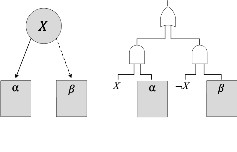
Figure 11. OBDD fragment and corresponding NNF circuit.

Ordered Binary Decision Diagrams (OBDDs).

SDDs subsume the well known Ordered Binary Decision Diagrams (OBDDs) and are exponentially more succinct than OBDDs (Bova, 2016); see also (Bollig and Buttkus, 2019). An OBDD is an ordered decision graph: the variables on every path from the root to a leaf ($0$ or $1$) respect a given variable order (Bryant, 1986; Meinel and Theobald, 1998; Wegener, 2000); see Figure 25. An OBDD node and its corresponding NNF fragment are depicted in Figure 11. As the figure shows, this fragment is also a multiplexer as in SDDs, except that we have precisely two primes which correspond to a variable and its negation. When an SDD is structured with respect to a right-linear vtree, the result is an OBDD; see Figure 10(c). SDDs and OBDDs can also be contrasted based on how they make decisions. An OBDD makes a decision based on the state of a binary variable and hence its decisions are always binary. An SDD makes decisions based on sentences (primes) so the corresponding number of decisions (subs) is not restricted to being binary.

The compilation of Boolean formula into tractable NNF circuits is done by systems known as knowledge compilers. Examples include c2d (Darwiche, 2004), cudd, mini-c2d (Oztok and Darwiche, 2014, 2018), d4 (Lagniez and Marquis, 2017), dsharp (Muise et al., 2012) and the sdd library (Choi and Darwiche, 2013). See also http://beyondnp.org/pages/solvers/knowledge-compilers/. A connection was made between model counters and knowledge compilers in (Huang and Darwiche, 2007), showing how model counters can be turned into knowledge compilers by keeping a trace of the exhaustive search they conduct on a Boolean formula. The dsharp compiler for d-DNNF (Muise et al., 2012) was the result of keeping a trace of the sharp-sat model counter (Thurley, 2006). While dedicated SAT solvers remain the state of the art for solving Sat, the state of the art for (weighted) model counting are either knowledge compilers or model counters whose traces are (subsets) of d-DNNF circuits.

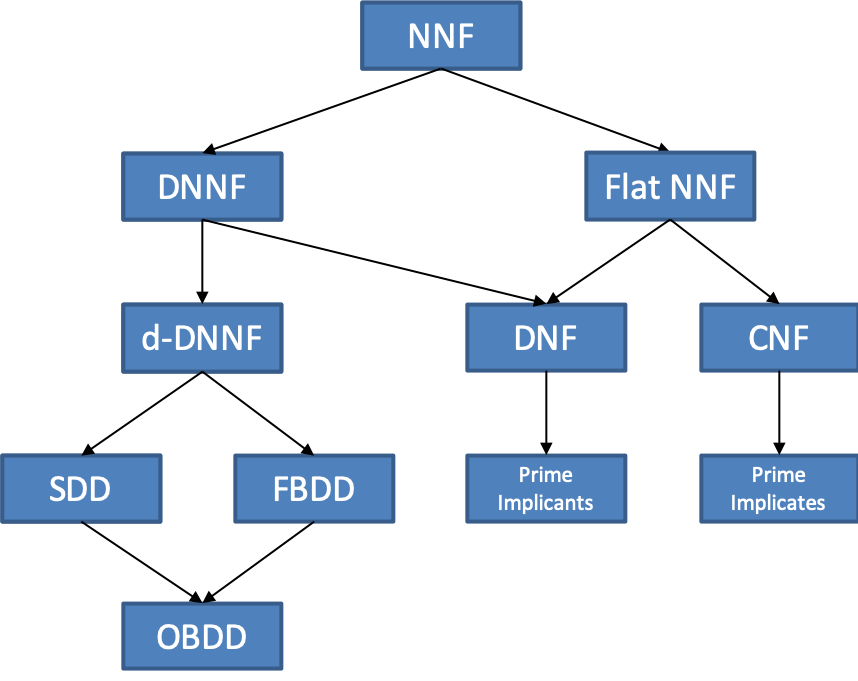
Figure 12. A partial taxonomy of NNF circuits.

Taxonomy of NNF circuits.

Figure 12 depicts a partial taxonomy of NNF circuits, most of which are tractable. A more comprehensive taxonomy was studied in (Darwiche and Marquis, 2002) under the term knowledge compilation map. A recent update on this map can be found in (Slivovsky, 2019), which includes recent results on the exponential separations between tractable NNF circuits.

Tractable NNF circuits were connected to, utilized by, and also benefited from other areas of computer science. This includes database theory, where connections were made to the notions of provenance and lineage, e.g., (Amarilli, 2019; Jha and Suciu, 2013). It also includes communication complexity, which led to sharper separation results between tractable NNF circuits, e.g., (Bova et al., 2016; Beame and Liew, 2015). Further applications to probabilistic reasoning and machine learning include the utilization of tractable circuits for uniform sampling (Sharma et al., 2018) and improving deep learning through the injection of symbolic knowledge; see, e.g., (Xu et al., 2018; Xie et al., 2019).

4. Logic For Learning From Data and Knowledge

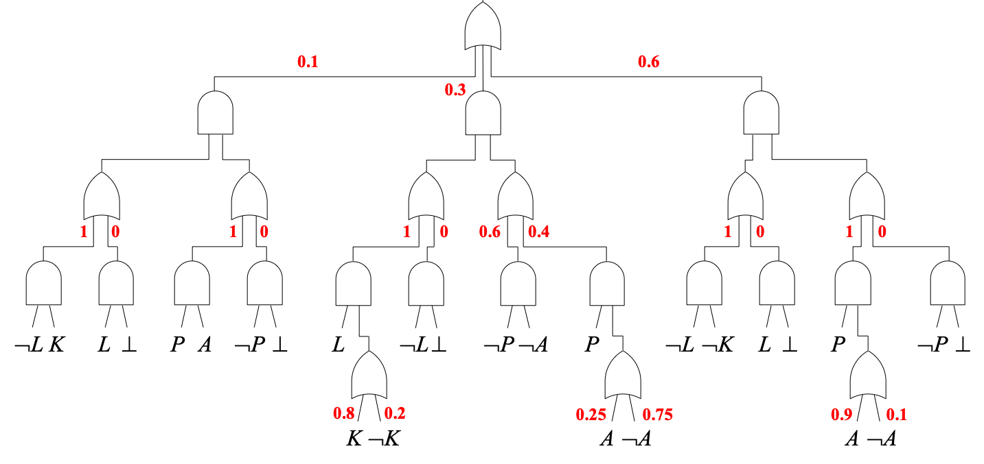
Figure 13. A probabilistic SDD circuit. The probabilities annotating inputs of or-gate are known as PSDD parameters.

Probabilistic Sentential Decision Diagrams (PSDDs).

The second role we consider for logic is in learning distributions from a combination of data and symbolic knowledge. This role has two dimensions: representational and computational. On the representational side, we use logic to eliminate situations that are impossible according to symbolic knowledge, which can reduce the amount of needed data and increase the robustness of learned representations. On the computational side, we use logic to factor the space of possible situations into a tractable NNF circuit so we can learn a distribution over the space and reason with it efficiently.

Consider the SDD circuit in Figure 13 which we showed earlier to have $9$ satisfying inputs out of $16$. Suppose that our goal is to induce a distribution on this space of satisfying circuit inputs. We can do this by simply assigning a distribution to each or-gate in the circuit as shown in Figure 13: each input of an or-gate is assigned a probability while ensuring that the probabilities assigned to the inputs add up to $1$. These local distributions are independent of one another. Yet, they are guaranteed to induce a normalized distribution over the space of satisfying circuit inputs. The resulting circuit is known as a probabilistic SDD circuit or a PSDD for short (Kisa et al., 2014).

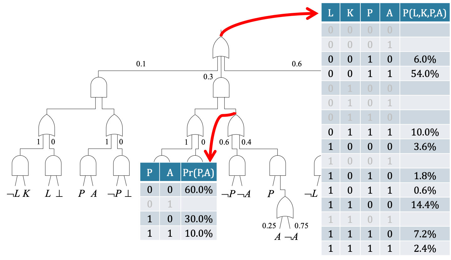
Figure 14. The compositional distributions of a PSDD circuit.

Semantics of PSDDs.

Given a PSDD with variables ${\bf X}$, the distribution ${\it Pr}({\bf X})$ it induces can be obtained as follows. To compute the probability of input ${\bf x}$ we perform a bottom-up pass on the circuit while assigning a value to each literal and gate output. The value of a literal is just its value in input ${\bf x}$ ($1$ or $0$). The value of an and-gate is the product of values assigned to its inputs. The value of an or-gate is the weighted sum of values assigned to its inputs (the weights are the probabilities annotating the gate inputs). The value assigned to the circuit output will then be the probability ${\it Pr}({\bf x})$. Figure 14 depicts the result of applying this evaluation process. As the figure shows, the probabilities of satisfying circuit inputs add up to $1$. Moreover, the probability of each unsatisfying input is $0$. The PSDD has a compositional semantics: each or-gate induces a distribution over the variables in the subcircuit rooted at the gate. Figure 14 depicts the distribution induced by an or-gate over variables $P$ and $A$.

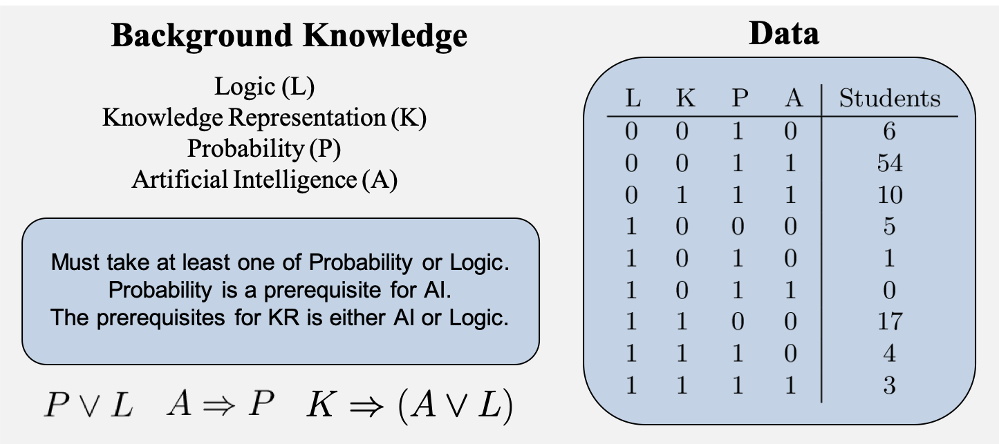
Figure 15. Learning from data and knowledge.

Learning from knowledge and data.

To see how PSDDs can be used to learn from a combination of data and symbolic knowledge, consider the example in Figure 15 from (Kisa et al., 2014). What we have here is a dataset that captures student enrollments in four courses offered by a computer science department. Each row in the dataset represents the number of students who have enrolled in the corresponding courses. Our goal is to learn a distribution from this data and the knowledge we have about the course prerequisites and requirements that is shown in Figure 15.

This symbolic knowledge can be captured by the propositional statement $(P\vee L)\wedge(A\Rightarrow P)\wedge(K\Rightarrow(A\vee L))$. The first step is to compile this knowledge into an SDD circuit. The SDD circuit in Figure 13 is actually the result of this compilation (using the vtree in Figure 10(a)). This SDD circuit will evaluate to $1$ for any course combination that is allowed by the prerequisites and requirements, otherwise it will evaluate to $0$. Our next step is to induce a distribution on the satisfying inputs of this course, that is, the valid course combinations. This can be done by learning a distribution for each or-gate in the SDD circuit, to yield a PSDD circuit.

The data in Figure 15 is complete in the sense that each row specifies precisely whether a course was enrolled into or not by the corresponding number of students. An incomplete dataset in this case would, for example, specify that $30$ students took logic, AI and probability, without specifying the status of enrollment in knowledge representation. If the data is complete, the maximum-likelihood parameters of a PSDD can be learned in time linear in the PSDD size. All we need to do is evaluate the SDD circuit for each example in the dataset, while keeping track of how many times a wire become high; see (Kisa et al., 2014) for details. The parameters shown in Figure 13 were actually learned using this procedure so the distribution they induce is the one guaranteed to maximize the probability of given data (under the chosen vtree).

Both MPE and MAR queries, discussed in Section 2, can be computed in time linear in the PSDD size (Kisa et al., 2014). Hence, not only can we estimate parameters efficiently under complete data, but we can also reason efficiently with the learned distribution. Finally, the PSDD is a complete and canonical representation of probability distributions. That is, PSDDs can represent any distribution, and there is a unique PSDD for that distribution (under some conditions) (Kisa et al., 2014).

PSDD circuits are based on the stronger versions of decomposability and determinism that underly SDD circuits. Probabilistic circuits that are based on the standard properties of decomposability and determinism are called ACs (Arithmetic Circuits) (Darwiche, 2003). Those based on decomposability only were introduced about ten years later and are known as SPNs (Sum-Product Networks) (Poon and Domingos, 2011). A treatment on the relative tractability and succinctness of these three circuit types can be found in (Choi and Darwiche, 2017; Shen et al., 2016).

4.1. Learning With Combinatorial Spaces

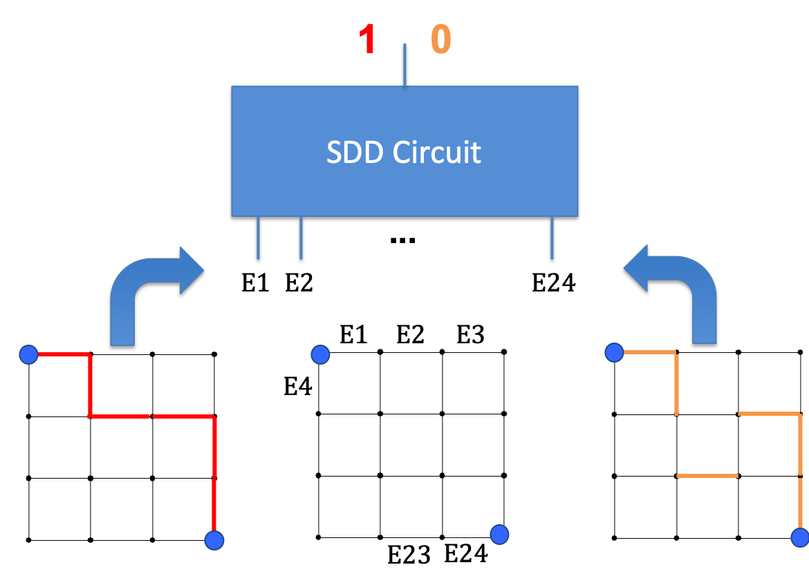
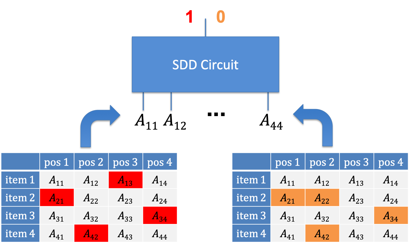
Figure 16. Encoding routes using SDDs. The red variable assignment (left) encoudes a valid route. The orange variable assignment (right) does not encode a valid route as the edges are disconnected.

Figure 17. Encoding rankings (total orderings) using SDDs. The red variable assignment (left) encodes a valid ranking. The orange variable assignment (right) does not encode a valid ranking (e.g., item $2$ appears in two positions).

Encoding combinatorial objects using SDDs.

We now discuss another type of symbolic knowledge that arises when learning distributions over combinatorial objects.

Consider Figures 17 and 17 which depicts two common types of combinatorial objects: routes and total orderings. In the case of routes, we have a map (in this case a grid for simplicity), a source and a destination. Our goal is to learn a distribution over the possible routes from the source to the destination given a dataset of routes, as discussed in (Choi et al., 2016). In the case of total orderings (rankings), we have $n$ items and we wish to learn a distribution over the possible rankings of these items, again from a dataset of rankings, as discussed in (Choi et al., 2015).

It is not uncommon to develop dedicated learning and inference algorithms when dealing with combinatorial objects. For example, a number of dedicated frameworks exist for learning and inference with distributions over rankings; see, e.g., (Mallows, 1957; Fligner and Verducci, 1986; Meila and Chen, 2010). What we will do, however, is show how learning and inference with combinatorial objects including rankings can be handled systematically using tractable circuits as proposed in (Choi et al., 2015, 2016; Shen et al., 2017; Choi et al., 2017b; Shen et al., 2019).

Consider the grid in Figure 17 (more generally, a map is modeled using an undirected graph). We can represent each edge $i$ in the map by a Boolean variable $E_{i}$ and each route as a variable assignment that sets only its corresponding edge variables to true. While every route can be represented by a variable assignment (e.g., the red route on the left of Figure 17), some assignments will correspond to invalid routes (e.g., the orange one on the right of Figure 17). One can construct a Boolean formula over edge variables whose satisfying assignments correspond precisely to valid (connected) routes and include additional constraints to keep only, for example, simple routes with no cycles; see (Choi et al., 2016; Nishino et al., 2017) for how this can be done.

After capturing the space of valid routes using an appropriate Boolean formula, we compile it to an SDD circuit. Circuit inputs that satisfy the SDD will then correspond to the space of valid routes; see Figure 17. A complete dataset in this case will be a multi-set of variable assignments, each corresponding to a taken route (obtained, for example, from GPS data). We can then learn PSDD parameters from this dataset and compiled SDD as done in (Choi et al., 2016, 2017b).

Figure 17 contains another example of applying this approach to learning distributions over rankings with $n$ items. In this case, we use $n^{2}$ Boolean variables $A_{ij}$ to encode a ranking, by setting variable $A_{ij}$ to true iff item $i$ is in position $j$. One can also construct a Boolean formula whose satisfying assignments correspond precisely to valid rankings. Compiling the formula to an SDD and then learning PSDD parameters from data allow us to learn a distribution over rankings that can be reasoned about efficiently. This proposal for rankings (and partial rankings, including tiers) was extended in (Choi et al., 2015), showing competitive results with some dedicated approaches for learning distributions over rankings. It also included an account for learning PSDD parameters from incomplete data and from structured data in which examples are expressed using arbitrary Boolean formula instead of just variable assignments.

A combinatorial probability space is a special case of the more general structured probability space, which is specified by a Boolean formula (i.e., the satisfying assignments need not correspond to combinatorial objects). The contrast is a standard probability space that is defined over all instantiations of a set of variables. We will use the term structured instead of combinatorial in the next section, as adopted in earlier works (Choi et al., 2015, 2016, 2017b; Shen et al., 2019), even as we continue to give examples from combinatorial spaces.

4.2. Conditional Spaces

We now turn to the notion of a conditional space: a structured space that is determined by the state of another space. The interest is in learning and reasoning with distributions over conditional spaces. This is a fundamental notion that arises in the context of causal probabilistic models, which require such conditional distributions when specifying probabilistic relationships between causes and effects. More generally, it arises in directed probabilistic graphical models, in which the graph specifies conditional independence relationships even though it may not have a causal interpretation.

A concrete example comes from the notion of a hierarchical map, which was introduced to better scale the compilation of maps into tractable circuits (Choi et al., 2017b; Shen et al., 2019). Figure 18 depicts an example of a three-level hierarchical map with a number of regions. It is a simplified map of neighborhoods in the Los Angeles Westside, where edges represent streets and nodes represent intersections. Nodes of the LA Westside have been partitioned into four sub-regions: Santa Monica, Westwood, Venice and Culver City. Westwood is further partitioned into two sub-regions: UCLA and Westwood Village.

The main intuition behind a hierarchical map is that navigation behavior in a region $R$ can become independent of navigation behavior in other regions, once we know how region $R$ was entered and exited. These independence relations are specified using a directed acyclic graph as shown in Figure 19 (called a cluster DAG in (Shen et al., 2018)). Consider the root node ‘Westside’ which contains variables $e_{1},\ldots,e_{6}$. These variables represent the roads used to cross between the four (immediate) sub-regions of the Westside. Once we know the state of these variables, we also know how each of these regions may have been entered and exited so their inner navigation behaviors become independent of one another.

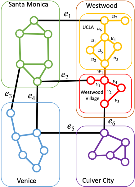
Figure 18. A three-level hierarchical map.

Hierarchical map.

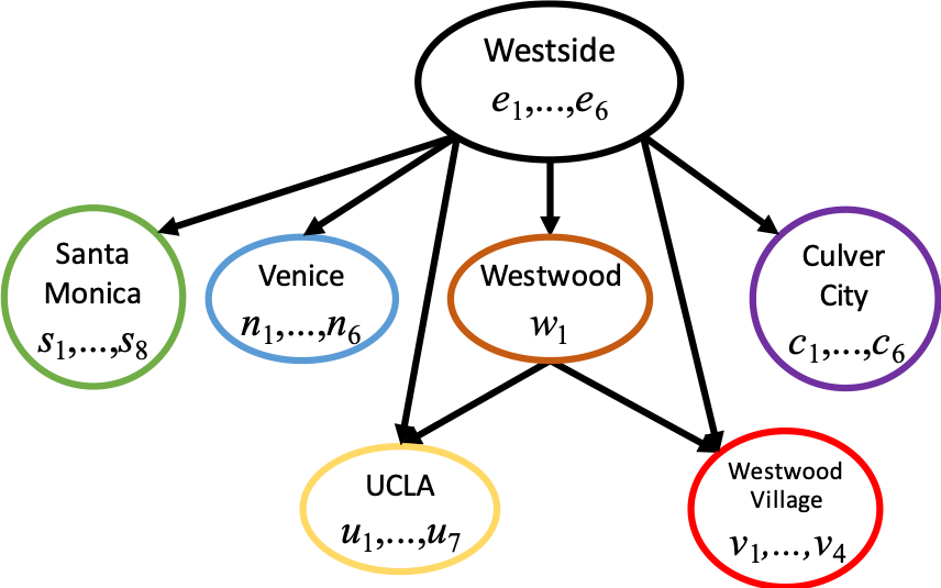
Figure 19. Specifying conditional independence relationships using a directed acyclic graph. The relationship between a node and its parent requires a conditional space.

Structured Bayesian network (SBN).

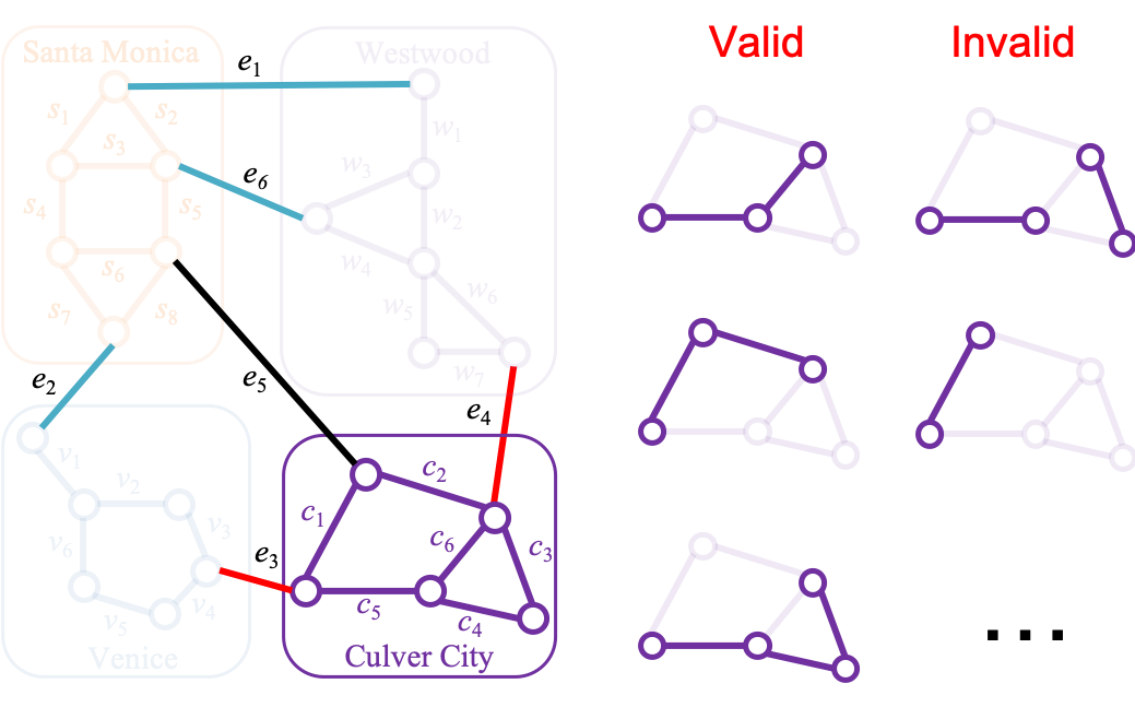
Figure 20. Illustrating the notion of a conditional space. The valid routes inside Culver City are a function of the Westside crossings we use to enter and exit the city.

Conditional spaces and structured probability spaces.

Let us now consider Figure 20 to see how the notion of a conditional space arises in this context. The figure highlights Culver City with streets $e_{1},\ldots,e_{6}$: the ones for crossing between regions in the Westside. What we need is a structured space over inner roads $c_{1},\ldots,c_{6}$ of Culver City that specifies valid routes inside the city. But this structured space depends on how we enter and exit the city, which is specified by another space over crossings $e_{1},\ldots,e_{6}$. That is, the structured space over Culver City roads is conditional on the space over Westside crossings.

The left of Figure 20 expands this example by illustrating the structured space over $c_{1},\ldots,c_{6}$ assuming we entered/existed Culver city using crossings $e_{3}$ and $e_{4}$ (highlighted in red). The illustration shows some variable assignments that belong to this structured space (valid) and some that do not (invalid). If we were to enter/exit Culver city using, say, crossings $e_{3}$ and $e_{5}$, then the structured space over $c_{1},\ldots,c_{6}$ would be different.

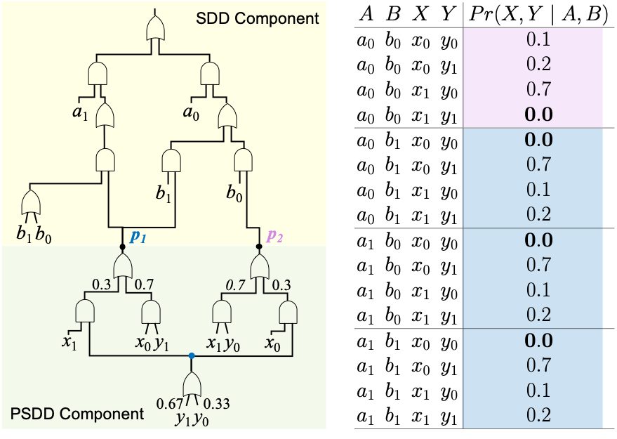
Figure 21. A conditional PSDD and the two conditional distributions it represents.

Conditional PSDD.

Figure 21 depicts a new class of tractable circuits, called conditional PSDDs, which can be used to induce distributions on conditional spaces (Shen et al., 2018). In this example, we have a structured space over variables $X,Y$ that is conditioned on a space over variables $A,B$. The conditional PSDD has two components: an SDD circuit (highlighted in yellow) and a multi-rooted PSDD (highlighted in green). The conditional distributions specified by this conditional PSDD are shown on the right of Figure 21. There are two of them: one for state $a_{0},b_{0}$ of variables $A,B$ and another for the remaining states. The structured space of the first distribution corresponds to the Boolean formula $x_{0}\vee y_{0}$. The structured space for the second distribution corresponds to $x_{1}\vee y_{1}$.

The semantics of a conditional PSDD is relatively simple and illustrated in Figure 24. Consider state $a_{0},b_{0}$ of variables $A,B$ (right of Figure 24). Evaluating the SDD component at this input leads to selecting the PSDD rooted at $p_{2}$, which generates the distribution conditioned on this state. Evaluating the SDD at any other state of variables $A,B$ leads to selecting the PSDD rooted at $p_{1}$, which generates the distribution for these states (left of Figure 24).

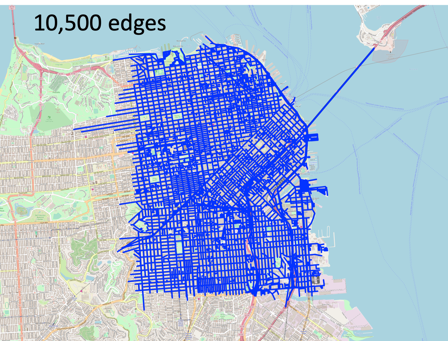
Figure 22. A map of downtown San Fransisco that was compiled into SDD/PSDD circuits.

Compiling maps into tractable circuits.

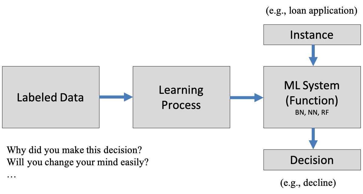
Figure 23. Reasoning about machine learning systems.

Explainable AI.

When a cluster DAG such as the one in Figure 19 is quantified using conditional PSDDs, the result is known as a structured Bayesian network (SBN) (Shen et al., 2018). The conditional PSDDs of an SBN can be multiplied together to yield a classical PSDD over network variables (Shen et al., 2016). To give a sense of practical complexity, the map of San Francisco depicted in Figure 22 has $10,500$ edges. A corresponding hierarchical map used in (Shen et al., 2019) was compiled into a PSDD with size of about $8.9$M (edges). The parameters of this SDD were learned from routes collected from GPS data and the induced distribution was used for several reasoning and classification tasks (Shen et al., 2019).

Figure 24. Selecting conditional distributions using the conditional PSDD of Figure 21.

Semantics of conditional PSDDs.

5. Logic For Meta Reasoning

We now turn to a most recent role for logic in AI: Reasoning about the behavior of machine learning systems.

Consider Figure 23 which depicts how most machine learning systems are constructed today. We have a labeled dataset that is used to learn a classifier, which is commonly a neural network, a Bayesian network classifier or a random forest. These classifiers are effectively functions that map instances to decisions. For example, an instance could be a loan application and the decision is whether to approve or decline the loan. There is now considerable interest in reasoning about the behavior of such systems. Explaining decisions is at the forefront of current interests: Why did you decline Maya’s application? Quantifying the robustness of these decisions is also attracting a lot of attention: Would reversing the decision on Maya require many changes to her application? In some domains, one expects the learned systems to satisfy certain properties, like monotonicity, and there is again an interest in proving such properties formally. For example, can we guarantee that a loan applicant will be approved when the only difference they have with another approved applicant is their higher income? These interests, however, are challenged by the numeric nature of machine learning systems and the fact that these systems are often model-free, e.g., neural networks, so they appear as black boxes that are hard to analyze.

The third role for logic we discuss next rests on the following observation: Even though these machine learning classifiers are learned from data and numeric in nature, they often implement discrete decision functions. One can therefore extract these decisions functions and represent them symbolically using tractable circuits. The outcome of this process is a circuit that precisely captures the input-output behavior of the machine learning system, which can then be used to reason about its behavior. This includes explaining decisions, measuring robustness and formally proving properties.

Consider the example in Figure 25 which pertains to one of the simplest machine learning systems: a Naive Bayes classifier. We have class variable $P$ and three features $B$, $U$ and $S$. Given an instance (patient) and their test results $b$, $u$ and $s$, this classifier renders a decision by computing the posterior probability ${\it Pr}(p|b,u,s)$ and then checking whether it passes a given threshold $T$. If it does, we declare a positive decision; otherwise, a negative decision.

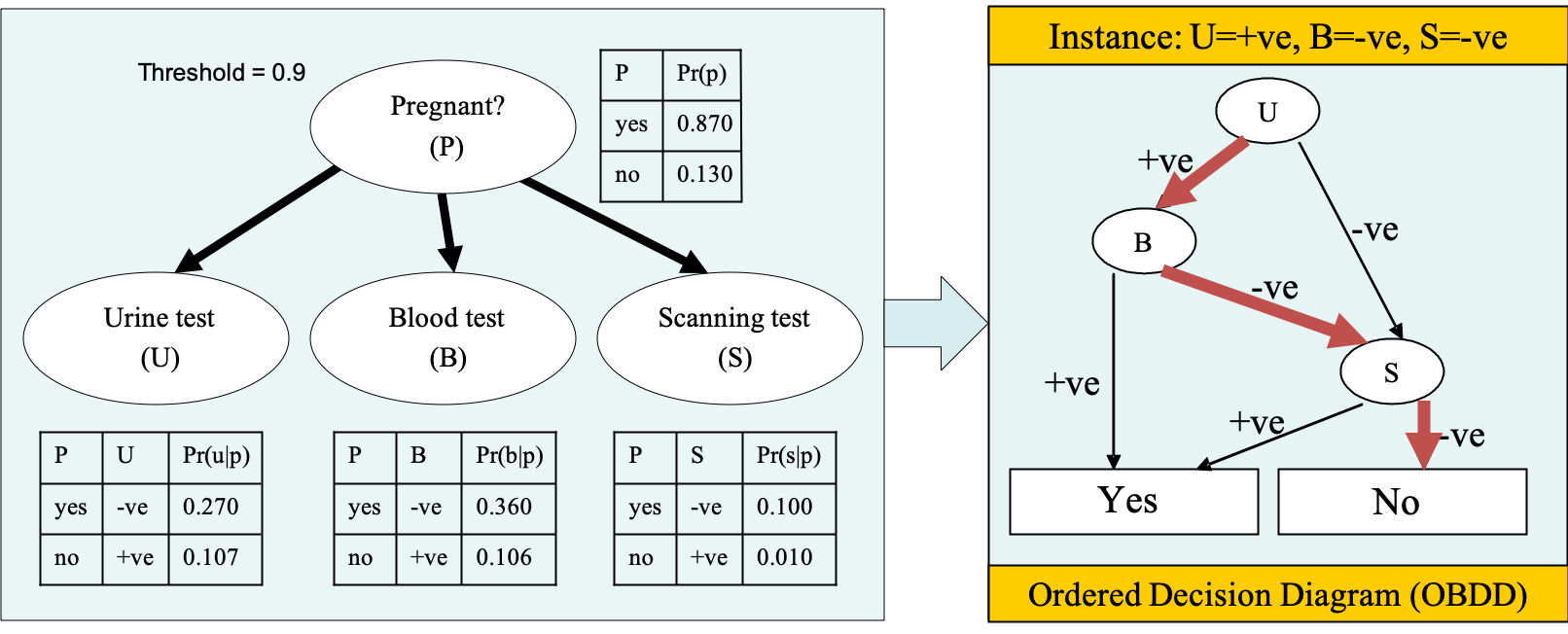
Figure 25. Compiling a Naive Bayes classifier into a symbolic decision graph (a tractable NNF circuit).

Compiling machine learning systems into circuits.

While this classifier is numeric and its decisions are based on probabilistic reasoning, it does induce a discrete decision function. In fact, the function is Boolean in this case as it maps the Boolean variables $B$, $U$ and $S$, which correspond to test results, into a binary decision. This observation was originally made in (Chan and Darwiche, 2003), which proposed the compilation of Naive Bayes classifiers into symbolic decision graphs as shown in Figure 25. For every instance, the decision made by the (probabilistic) naive Bayes classifier is guaranteed to be the same as the one made by the (symbolic) decision graph.

The compilation algorithm of (Chan and Darwiche, 2003) generates Ordered Decision Diagrams (ODDs), which correspond to Ordered Binary Decision Diagrams (OBDDs) when the features are binary. Recall from Figure 11 that an OBDD corresponds to a tractable NNF circuit (once one adjusts for notation). Hence, the proposal in (Chan and Darwiche, 2003) amounted to compiling a Naive Bayes classifier into a tractable NNF circuit that precisely captures its input-output behavior. This compilation algorithm was recently extended to Bayesian network classifiers with tree structures (Shih et al., 2018b) and later to Bayesian network classifiers with arbitrary structures (Shih et al., 2019a). Certain classes of neural networks can also be compiled into tractable circuits, which include SDD circuits as shown in (Choi et al., 2019; Shih et al., 2019b; Shi et al., 2020).

While Bayesian and neural networks are numeric in nature, random forests are not (at least the ones with majority voting). Hence, random forests represent less of a challenge for this role of logic as we can easily encode the input-output behavior of a random forest using a Boolean formula. We first encode each decision tree into a Boolean formula, which is straightforward even in the presence of continuous variables (the learning algorithm discretizes the variables). We then combine these formulas using a majority circuit. The remaining challenge is purely computational as we now need to compile the Boolean formula into a suitable tractable circuit.

We next turn to reasoning about the behavior of classifiers, assuming they have been compiled into tractable circuits.

5.1. Explaining Decisions

Consider the classifier in Figure 25 and Susan who tested positive for the blood, urine and scanning tests. The classifier says that Susan is pregnant and we need to know why.

The first notion to address this question is the PI-explanation introduced in (Shih et al., 2018b) and termed sufficient reason in (Darwiche and Hirth, 2020) (to make distinctions with other types of reasons). A sufficient reason is a minimal set of instance characteristics that is guaranteed to trigger the decision, regardless of what the other characteristics might be. In this example, Susan would be classified as pregnant as long as she tests positive for the scanning test; that is, regardless of what the other two test results are. Hence, $S\!=\!{+ve}$ is a sufficient reason for the decision. There is only one other sufficient reason for this decision: $B\!=\!{+ve},\>U\!=\!{+ve}$. Combining the two sufficient reasons we get $S\!=\!{+ve}\vee(B\!=\!{+ve},\>U\!=\!{+ve})$, which is called the complete reason behind the decision (Darwiche and Hirth, 2020) or simply the decision’s reason.

The reason behind a decision provides the most general abstraction of an instance that can trigger the decision. Any instance property that can trigger the decision is captured by the reason. The reason behind a decision can also be used to decide whether the decision is biased, and in some cases whether the classifier itself is biased even when the considered decision is not. We will provide concrete examples later but we first need to establish the semantics of sufficient and complete reasons.

Figure 26. Prime implicants of Boolean functions.

Prime implicants.

These notions are based on prime implicants of Boolean functions, which have been studied extensively in the literature (Crama and Hammer, 2011; Quine, 1952; McCluskey, 1956; Quine, 1959). Consider the Boolean function $f$ in Figure 26 over variables $A$, $B$ and $C$. A prime implicant of the function is a minimal setting of its variables that causes the function to trigger. This function has three prime implicants as shown in the figure: $AB$, $AC$ and $B\overline{C}$. Consider now the instance $AB\overline{C}$ leading to a positive decision $f(AB\overline{C})=1$. The sufficient reasons for this decision are the prime implicants of function $f$ that are compatible with the instance: $AB$ and $B\overline{C}$. Explaining negative decisions requires working with the function’s complement $\overline{f}$. Consider instance $\overline{A}BC$, which sets the function to $0$. The complement $\overline{f}$ has three prime implicants $\overline{A}C$, $\overline{B}\,\overline{C}$ and $\overline{A}\,\overline{B}$. Only one of these is compatible with the instance, $\overline{A}C$, so it is the only sufficient reason for the decision on this instance.

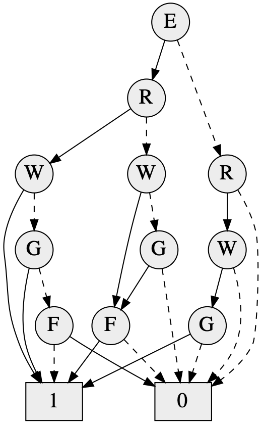
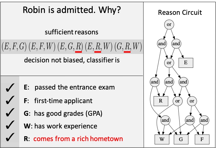
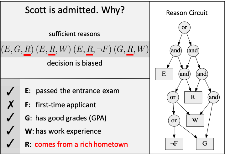
Figure 27. Explaining admission decisions of an OBDD classifier (left). The reason circuit represents the complete reason behind a decision (a disjunction of all its sufficient reasons). The reason circuit is monotone and hence tractable.

Explaining decisions of machine learning systems.

Sufficient reasons can be used to reason about decision and classifier bias, which are defined in the context of protected features. A decision on an instance is biased iff it would be different had we only changed protected features in the instance. A classifier is biased iff it makes at least one biased decision. If every sufficient reason of a decision contains at least one protected feature, the decision is guaranteed to be biased (Darwiche and Hirth, 2020). If some but not all sufficient reasons contain protected features, the decision is not biased but the classifier is guaranteed to be biased (that is, the classifier will make a biased decision on some other instance).

Consider Figure 27 which depicts an admissions classifier in the form of an OBDD (the classifier could have been compiled from a Bayesian network, a neural network or a random forest). The classifier has five features, one of them is protected: whether the applicant comes from a rich hometown ($R$). Robin is admitted by the classifier and the decision has five sufficient reasons, depicted in Figure 27. Three of these sufficient reasons contain the protected feature $R$ and two do not. Hence, the decision on Robin is not biased, but the classifier is biased. Consider now Scott who is also admitted. The decision on Scott has four sufficient reasons and all of them contain a protected feature. Hence, the decision on Scott is biased: it will be reversed if Scott were not to come from a rich hometown.

A decision may have an exponential number of reasons, which makes it impractical to analyze decisions by enumerating sufficient reasons. One can use the complete reason behind a decision for this purpose as it contains all the needed information. Moreover, if the classifier is represented by an appropriate tractable circuit, then the complete reason behind a decision can be extracted from the classifier in linear time, in the form of another tractable circuit called the reason circuit (Darwiche and Hirth, 2020). Figure 27 depicts the reason circuits for decisions on Robin and Scott. Reason circuits get their tractability from being monotone, allowing one to efficiently reason about decisions including their bias. One can also reason about counterfactuals once the reason circuit for a decision is constructed. For example, one can efficiently evaluate statements such as: The decision on April would stick even if she were not to have work experience because she passed the entrance exam; see (Darwiche and Hirth, 2020) for details.

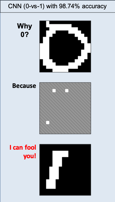
Figure 28. Explaining the decisions of a neural network.

Explaining decisions of neural networks.

We conclude this section by pointing to an example from (Shi et al., 2020), which compiled a Convolutional Neural Network (CNN) that classifies digits $0$ and $1$ in $16\times 16$ images. The CNN had an accuracy of $98.74\%$. Figure 28 depicts an image that was classified correctly as containing digit $0$. One of the sufficient reasons for this decision is also shown in the figure, which includes only $3$ pixels out of $256$. If these three pixels are kept white, the CNN will classify the image as containing digit $0$ regardless of the state of other pixels.

5.2. Robustness and Formal Properties

One can define both decision and model robustness. The robustness of a decision is defined as the smallest number of features that need to flip before the decision flips (Shih et al., 2018a). Model robustness is defined as the average decision robustness (over all possible instances) (Shi et al., 2020). Decision robustness is $co{\mathsf{NP}}$-complete and model robustness is $\#\mathsf{P}$-hard. If the decision function is represented using a tractable circuit of a suitable type, which includes OBDDs, then decision robustness can be computed in time linear in the circuit size (Shih et al., 2018a). Model robustness can be computed using a sequence of polytime operations but the total complexity is not guaranteed to be in polytime (Shi et al., 2020).

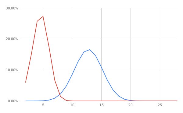
Figure 29. Robustness level vs. proportion of instances for two neural networks with similar accuracies. Net $1$ is plotted in blue (right) and Net $2$ in red (left).

Robustness of neural networks.

Figure 29 depicts an example of robustness analysis for two CNNs that classify digits $1$ and $2$ in $16\times 16$ images (Shi et al., 2020). The two CNNs have the same architectures but were trained using two different parameter seeds, leading to testing accuracies of $98.18$ (Net $1$) and $96.93$ (Net $2$). The CNNs were compiled into SDD circuits where the SDD of Net $1$ had $3,653$ edges and the one for Net $2$ had only $440$ edges. The two CNNs are similar in terms of accuracy (differing by only $1.25\%$) but are very different when compared by robustness. For example, Net $1$ attained a model robustness of $11.77$ but Net $2$ obtained a robustness of only $3.62.$ For Net $2$, this means that on average, $3.62$ pixel flips are needed to flip a digit-$1$ classification to digit-$2$, or vice versa. Moreover, the maximum robustness of Net $1$ was $27$, while that of Net $2$ was only $13.$ For Net $1$, this means that there is an instance that would not flip classification unless one is allowed to flip at least $27$ of its pixels. For Net $2$, it means the decision on any instance can be flipped if one is allowed to flip $13$ or more pixels. Note that Figure 29 reports the robustness of $2^{256}$ instances for each CNN, which is made possible by having captured the input-output behavior of these CNNs using tractable circuits.

In the process of compiling a neural network into a tractable circuit as proposed in (Choi et al., 2019; Shi et al., 2020), one also compiles each neuron into its own tractable circuit. This allows one to interpret the functionality of each neuron by analyzing the corresponding tractable circuit, which is a function of the network’s inputs. For example, if the tractable circuit supports model counting in polytime, then one can efficiently answer questions such as: Of all network inputs that cause a neuron to fire, what proportion of them set input $X_{i}$ to $1$? This is just one mode of analysis that can be performed efficiently once the input-output behavior of a machine learning system is compiled into a suitable tractable circuit. Other examples include monotonicity analysis, which is discussed in (Shih et al., 2018a).

6. Conclusion and Outlook

We reviewed three modern roles for logic in artificial intelligence: logic as a basis for computation, logic for learning from a combination of data and knowledge, and logic for reasoning about the behavior of machine learning systems.

Everything we discussed was contained within the realm of propositional logic and based on the theory of tractable Boolean circuits. The essence of these roles is based on an ability to compile Boolean formula into Boolean circuits with appropriate properties. As such, the bottleneck for advancing these roles further—at least as far as enabling more scalable applications—boils down to the need for improving the effectiveness of knowledge compilers (i.e., algorithms that enforce certain properties on NNF circuits). The current work on identifying (more) tractable circuits and further studying their properties appears to be ahead of work on improving compilation algorithms. This imbalance needs to be addressed, perhaps by encouraging more open source releases of knowledge compilers and the nurturing of regular competitions as has been done successfully by the SAT community.

McCarthy’s proposal for using logic as the basis for knowledge representation and reasoning had an overwhelming impact (McCarthy, 1959). But it also entrenched into our thinking a role for logic that has now been surpassed, while continuing to be the dominant role associated with logic in textbooks on artificial intelligence. Given the brittleness of purely symbolic representations in key applications, and the dominance today of learned, numeric representations, this entrenched association has pushed logic to a lower priority in artificial intelligence research than what can be rationally justified.

Another major (and more recent) transition relates to the emergence of machine learning “boxes,” which have expanded the scope and utility of symbolic representations and reasoning. While symbolic representations may be too brittle to fully represent certain aspects of the real world, they are provably sufficient for representing the behavior of certain machine learning boxes (and exactly when the box’s inputs/outputs are discrete). This has created a new role for logic in “reasoning about what was learned” in contrast to the older and entrenched role of reasoning about the real world.

The latter transition is more significant than may appear on first sight. For example, the behavior of a machine learning box is driven by the box’s internal causal mechanisms and can therefore be subjected to causal reasoning and analysis—even when the box itself was built using ad hoc techniques and may have therefore missed on capturing causality of the real world. Machine learning boxes, called “The AI” by many today, are now additional inhabitants of the real world. As such, they should be viewed as a new “subject” of logical and causal reasoning perhaps more so than their competitor.

These modern transitions—and the implied new modes of interplay between logic, probabilistic reasoning and machine learning—need to be paralleled by a transition in AI education that breaks away from the older models of viewing these areas as being either in competition or merely in modular harmony. What we need here is not only integration of these methods but also their fusion. Quoting (Darwiche, 2018): “We need a new generation of AI researchers who are well versed in and appreciate classical AI, machine learning, and computer science more broadly while also being informed about AI history.” Cultivating such a generation of AI researchers is another bottleneck to further advance the modern roles of logic in AI and to further advance the field of AI as a whole.

- (1)
- Amarilli (2019) Antoine Amarilli. 2019. Provenance in Databases and Links to Knowledge Compilation. In KOCOON workshop on knowledge compilation. http://kocoon.gforge.inria.fr/slides/amarilli.pdf.
- Beame and Liew (2015) Paul Beame and Vincent Liew. 2015. New Limits for Knowledge Compilation and Applications to Exact Model Counting. In UAI. AUAI Press, 131–140.
- Bollig and Buttkus (2019) Beate Bollig and Matthias Buttkus. 2019. On the Relative Succinctness of Sentential Decision Diagrams. Theory Comput. Syst. 63, 6 (2019), 1250–1277.
- Boutilier et al. (1996) Craig Boutilier, Nir Friedman, Moisés Goldszmidt, and Daphne Koller. 1996. Context-Specific Independence in Bayesian Networks. In UAI. 115–123.
- Bova (2016) Simone Bova. 2016. SDDs Are Exponentially More Succinct than OBDDs. In AAAI. 929–935.
- Bova et al. (2016) Simone Bova, Florent Capelli, Stefan Mengel, and Friedrich Slivovsky. 2016. Knowledge Compilation Meets Communication Complexity. In IJCAI. IJCAI/AAAI Press, 1008–1014.
- Bryant (1986) Randal E. Bryant. 1986. Graph-Based Algorithms for Boolean Function Manipulation. IEEE Trans. Computers 35, 8 (1986), 677–691.
- Cadoli and Donini (1997) Marco Cadoli and Francesco M. Donini. 1997. A Survey on Knowledge Compilation. AI Commun. 10, 3,4 (1997), 137–150.
- Chan and Darwiche (2003) Hei Chan and Adnan Darwiche. 2003. Reasoning About Bayesian Network Classifiers. In Proceedings of the Nineteenth Conference on Uncertainty in Artificial Intelligence (UAI). 107–115.
- Chavira and Darwiche (2008) Mark Chavira and Adnan Darwiche. 2008. On Probabilistic Inference by Weighted Model Counting. Artificial Intelligence 172, 6–7 (April 2008), 772–799.
- Chen et al. (2015) Suming Jeremiah Chen, Arthur Choi, and Adnan Darwiche. 2015. Value of Information Based on Decision Robustness. In AAAI. AAAI Press, 3503–3510.
- Choi and Darwiche (2013) Arthur Choi and Adnan Darwiche. 2013. Dynamic Minimization of Sentential Decision Diagrams. In Proceedings of the 27th Conference on Artificial Intelligence (AAAI).
- Choi and Darwiche (2017) Arthur Choi and Adnan Darwiche. 2017. On Relaxing Determinism in Arithmetic Circuits. In Proceedings of the Thirty-Fourth International Conference on Machine Learning (ICML). 825–833.
- Choi et al. (2017b) Arthur Choi, Yujia Shen, and Adnan Darwiche. 2017b. Tractability in Structured Probability Spaces. In NIPS.
- Choi et al. (2019) Arthur Choi, Weijia Shi, Andy Shih, and Adnan Darwiche. 2019. Compiling Neural Networks into Tractable Boolean Circuits. In AAAI Spring Symposium on Verification of Neural Networks (VNN).
- Choi et al. (2016) Arthur Choi, Nazgol Tavabi, and Adnan Darwiche. 2016. Structured Features in Naive Bayes Classification. In AAAI.
- Choi et al. (2015) Arthur Choi, Guy Van den Broeck, and Adnan Darwiche. 2015. Tractable Learning for Structured Probability Spaces: A Case Study in Learning Preference Distributions. In IJCAI.
- Choi et al. (2012) Arthur Choi, Yexiang Xue, and Adnan Darwiche. 2012. Same-Decision Probability: A Confidence Measure for Threshold-Based Decisions. International Journal of Approximate Reasoning (IJAR) 53, 9 (2012), 1415–1428.
- Choi et al. (2017a) YooJung Choi, Adnan Darwiche, and Guy Van den Broeck. 2017a. Optimal Feature Selection for Decision Robustness in Bayesian Networks. In IJCAI. ijcai.org, 1554–1560.
- Choi and den Broeck (2018) YooJung Choi and Guy Van den Broeck. 2018. On Robust Trimming of Bayesian Network Classifiers. In IJCAI. ijcai.org, 5002–5009.
- Crama and Hammer (2011) Yves Crama and Peter L. Hammer. 2011. Boolean Functions - Theory, Algorithms, and Applications. Encyclopedia of mathematics and its applications, Vol. 142. Cambridge University Press.
- Darwiche (2001a) Adnan Darwiche. 2001a. Decomposable Negation Normal Form. J. ACM 48, 4 (2001), 608–647.
- Darwiche (2001b) Adnan Darwiche. 2001b. On the Tractable Counting of Theory Models and its Application to Truth Maintenance and Belief Revision. Journal of Applied Non-Classical Logics 11, 1-2 (2001), 11–34.
- Darwiche (2002) Adnan Darwiche. 2002. A Logical Approach to Factoring Belief Networks. In KR. 409–420.
- Darwiche (2003) Adnan Darwiche. 2003. A Differential Approach to Inference in Bayesian Networks. JACM 50, 3 (2003), 280–305.
- Darwiche (2004) Adnan Darwiche. 2004. New Advances in Compiling CNF into Decomposable Negation Normal Form. In ECAI. 328–332.
- Darwiche (2009) Adnan Darwiche. 2009. Modeling and Reasoning with Bayesian Networks. Cambridge University Press.
- Darwiche (2011) Adnan Darwiche. 2011. SDD: A New Canonical Representation of Propositional Knowledge Bases. In IJCAI. 819–826.
- Darwiche (2014) Adnan Darwiche. 2014. Tractable Knowledge Representation Formalisms. In Tractability, Lucas Bordeaux, Youssef Hamadi, and Pushmeet Kohli (Eds.). Cambridge University Press, 141–172.
- Darwiche (2018) Adnan Darwiche. 2018. Human-level intelligence or animal-like abilities? Commun. ACM 61, 10 (2018), 56–67.
- Darwiche and Choi (2010) Adnan Darwiche and Arthur Choi. 2010. Same-Decision Probability: A Confidence Measure for Threshold-Based Decisions under Noisy Sensors. In Proceedings of the Fifth European Workshop on Probabilistic Graphical Models (PGM). 113–120.
- Darwiche et al. (2008) Adnan Darwiche, Rina Dechter, Arthur Choi, Vibhav Gogate, and Lars Otten. 2008. Results from the Probabilistic Inference Evaluation of UAI-08. (2008).
- Darwiche and Hirth (2020) Adnan Darwiche and Auguste Hirth. 2020. On The Reasons Behind Decisions. In Proceedings of the 24th European Conference on Artificial Intelligence (ECAI).
- Darwiche and Marquis (2002) Adnan Darwiche and Pierre Marquis. 2002. A knowledge compilation map. JAIR 17 (2002), 229–264.
- Dries et al. (2015) Anton Dries, Angelika Kimmig, Wannes Meert, Joris Renkens, Guy Van den Broeck, Jonas Vlasselaer, and Luc De Raedt. 2015. ProbLog2: Probabilistic Logic Programming. In ECML/PKDD (3) (Lecture Notes in Computer Science), Vol. 9286. Springer, 312–315.
- Fligner and Verducci (1986) Michael A Fligner and Joseph S Verducci. 1986. Distance based ranking models. Journal of the Royal Statistical Society. Series B (Methodological) (1986), 359–369.
- Huang et al. (2006) Jinbo Huang, Mark Chavira, and Adnan Darwiche. 2006. Solving MAP Exactly by Searching on Compiled Arithmetic Circuits. In AAAI. 1143–1148.
- Huang and Darwiche (2007) Jinbo Huang and Adnan Darwiche. 2007. The Language of Search. J. Artif. Intell. Res. (JAIR) 29 (2007), 191–219.
- Ignatiev et al. (2019a) Alexey Ignatiev, Nina Narodytska, and João Marques-Silva. 2019a. Abduction-Based Explanations for Machine Learning Models. In Proceedings of the Thirty-Third Conference on Artificial Intelligence (AAAI). 1511–1519.
- Ignatiev et al. (2019b) Alexey Ignatiev, Nina Narodytska, and João Marques-Silva. 2019b. On Relating Explanations and Adversarial Examples. In Advances in Neural Information Processing Systems 32 (NeurIPS). 15857–15867.
- Ignatiev et al. (2019c) Alexey Ignatiev, Nina Narodytska, and João Marques-Silva. 2019c. On Validating, Repairing and Refining Heuristic ML Explanations. CoRR abs/1907.02509 (2019).
- Jha and Suciu (2013) Abhay Kumar Jha and Dan Suciu. 2013. Knowledge Compilation Meets Database Theory: Compiling Queries to Decision Diagrams. Theory Comput. Syst. 52, 3 (2013), 403–440.
- Katz et al. (2017) Guy Katz, Clark W. Barrett, David L. Dill, Kyle Julian, and Mykel J. Kochenderfer. 2017. Reluplex: An Efficient SMT Solver for Verifying Deep Neural Networks. In Computer Aided Verification CAV. 97–117.
- Kisa et al. (2014) Doga Kisa, Guy Van den Broeck, Arthur Choi, and Adnan Darwiche. 2014. Probabilistic Sentential Decision Diagrams. In KR.
- Koller and Friedman (2009) D. Koller and N. Friedman. 2009. Probabilistic Graphical Models: Principles and Techniques. MIT Press.
- Lagniez and Marquis (2017) Jean-Marie Lagniez and Pierre Marquis. 2017. An Improved Decision-DNNF Compiler. In IJCAI. ijcai.org, 667–673.
- Latour et al. (2017) Anna L. D. Latour, Behrouz Babaki, Anton Dries, Angelika Kimmig, Guy Van den Broeck, and Siegfried Nijssen. 2017. Combining Stochastic Constraint Optimization and Probabilistic Programming - From Knowledge Compilation to Constraint Solving. In CP (Lecture Notes in Computer Science), Vol. 10416. Springer, 495–511.
- Leofante et al. (2018) Francesco Leofante, Nina Narodytska, Luca Pulina, and Armando Tacchella. 2018. Automated Verification of Neural Networks: Advances, Challenges and Perspectives. CoRR abs/1805.09938 (2018).
- Mallows (1957) Colin L. Mallows. 1957. Non-null ranking models. Biometrika (1957).
- Manhaeve et al. (2018) Robin Manhaeve, Sebastijan Dumancic, Angelika Kimmig, Thomas Demeester, and Luc De Raedt. 2018. DeepProbLog: Neural Probabilistic Logic Programming. In Advances in Neural Information Processing Systems 31, S. Bengio, H. Wallach, H. Larochelle, K. Grauman, N. Cesa-Bianchi, and R. Garnett (Eds.). Curran Associates, Inc., 3749–3759. http://papers.nips.cc/paper/7632-deepproblog-neural-probabilistic-logic-programming.pdf
- Marquis (1995) Pierre Marquis. 1995. Knowledge Compilation Using Theory Prime Implicates. In IJCAI. 837–845.
- McCarthy (1959) John McCarthy. 1959. Programs with common sense. In Proceedings of the Teddington Conference on the Mechanization of Thought Processes. http://www-formal.stanford.edu/jmc/mcc59.html.
- McCluskey (1956) E. J. McCluskey. 1956. Minimization of Boolean functions. The Bell System Technical Journal 35, 6 (Nov 1956), 1417–1444. https://doi.org/10.1002/j.1538-7305.1956.tb03835.x
- Meila and Chen (2010) Marina Meila and Harr Chen. 2010. Dirichlet process mixtures of generalized Mallows models. In Proceedings of UAI.
- Meinel and Theobald (1998) Christoph Meinel and Thorsten Theobald. 1998. Algorithms and Data Structures in VLSI Design: OBDD - Foundations and Applications. Springer.
- Muise et al. (2012) Christian J. Muise, Sheila A. McIlraith, J. Christopher Beck, and Eric I. Hsu. 2012. Dsharp: Fast d-DNNF Compilation with sharpSAT. In Canadian Conference on AI (Lecture Notes in Computer Science), Vol. 7310. Springer, 356–361.
- Murphy (2012) Kevin Patrick Murphy. 2012. Machine Learning: A Probabilistic Perspective. MIT Press.
- Narodytska et al. (2018) Nina Narodytska, Shiva Prasad Kasiviswanathan, Leonid Ryzhyk, Mooly Sagiv, and Toby Walsh. 2018. Verifying Properties of Binarized Deep Neural Networks. In Proceedings of the Thirty-Second AAAI Conference on Artificial Intelligence (AAAI).
- Nilsson (1986) N.J. Nilsson. 1986. Probabilistic logic. Artificial intelligence 28, 1 (1986), 71–87.
- Nishino et al. (2017) Masaaki Nishino, Norihito Yasuda, Shin-ichi Minato, and Masaaki Nagata. 2017. Compiling Graph Substructures into Sentential Decision Diagrams. In AAAI. 1213–1221.
- Oztok et al. (2016) Umut Oztok, Arthur Choi, and Adnan Darwiche. 2016. Solving PPPP-Complete Problems Using Knowledge Compilation. In Proceedings of the 15th International Conference on Principles of Knowledge Representation and Reasoning (KR). 94–103.
- Oztok and Darwiche (2014) Umut Oztok and Adnan Darwiche. 2014. On Compiling CNF into Decision-DNNF. In CP. 42–57.
- Oztok and Darwiche (2018) Umut Oztok and Adnan Darwiche. 2018. An Exhaustive DPLL Algorithm for Model Counting. J. Artif. Intell. Res. 62 (2018), 1–32.
- Park and Darwiche (2004) James D. Park and Adnan Darwiche. 2004. Complexity Results and Approximation Strategies for MAP Explanations. J. Artif. Intell. Res. (JAIR) 21 (2004), 101–133.
- Pearl (1988) J. Pearl. 1988. Probabilistic Reasoning in Intelligent Systems: Networks of Plausible Inference. Morgan Kaufmann.
- Pipatsrisawat and Darwiche (2008) Knot Pipatsrisawat and Adnan Darwiche. 2008. New Compilation Languages Based on Structured Decomposability. In AAAI. 517–522.
- Pipatsrisawat and Darwiche (2009) Knot Pipatsrisawat and Adnan Darwiche. 2009. A New d-DNNF-Based Bound Computation Algorithm for Functional EMAJSAT. In IJCAI. 590–595.
- Poon and Domingos (2011) Hoifung Poon and Pedro M. Domingos. 2011. Sum-Product Networks: A New Deep Architecture. In UAI. 337–346.
- Quine (1952) W. V. Quine. 1952. The Problem of Simplifying Truth Functions. The American Mathematical Monthly 59, 8 (1952), 521–531. http://www.jstor.org/stable/2308219
- Quine (1959) W. V. Quine. 1959. On Cores and Prime Implicants of Truth Functions. The American Mathematical Monthly 66, 9 (1959), 755–760. http://www.jstor.org/stable/2310460
- Ribeiro et al. (2018) Marco Túlio Ribeiro, Sameer Singh, and Carlos Guestrin. 2018. Anchors: High-Precision Model-Agnostic Explanations. In AAAI. AAAI Press, 1527–1535.
- Roth (1996) Dan Roth. 1996. On the Hardness of Approximate Reasoning. AIJ 82, 1-2 (1996), 273–302.
- Sang et al. (2005) Tian Sang, Paul Beame, and Henry A. Kautz. 2005. Performing Bayesian Inference by Weighted Model Counting. In AAAI. 475–482.
- Selman and Kautz (1996) Bart Selman and Henry A. Kautz. 1996. Knowledge Compilation and Theory Approximation. JACM 43, 2 (1996), 193–224.
- Sharma et al. (2018) Shubham Sharma, Rahul Gupta, Subhajit Roy, and Kuldeep S. Meel. 2018. Knowledge Compilation meets Uniform Sampling. In LPAR (EPiC Series in Computing), Vol. 57. EasyChair, 620–636.
- Shen et al. (2016) Yujia Shen, Arthur Choi, and Adnan Darwiche. 2016. Tractable Operations for Arithmetic Circuits of Probabilistic Models. In Advances in Neural Information Processing Systems 29 (NIPS).
- Shen et al. (2017) Yujia Shen, Arthur Choi, and Adnan Darwiche. 2017. A Tractable Probabilistic Model for Subset Selection. In Proceedings of the 33rd Conference on Uncertainty in Artificial Intelligence (UAI).
- Shen et al. (2018) Yujia Shen, Arthur Choi, and Adnan Darwiche. 2018. Conditional PSDDs: Modeling and Learning With Modular Knowledge. In AAAI. AAAI Press, 6433–6442.
- Shen et al. (2019) Yujia Shen, Anchal Goyanka, Adnan Darwiche, and Arthur Choi. 2019. Structured Bayesian Networks: From Inference to Learning with Routes. In AAAI. AAAI Press, 7957–7965.
- Shi et al. (2020) Weijia Shi, Andy Shih, Adnan Darwiche, and Arthur Choi. 2020. On Tractable Representations of Binary Neural Networks. http://arxiv.org/abs/2004.02082.
- Shih et al. (2018a) Andy Shih, Arthur Choi, and Adnan Darwiche. 2018a. Formal Verification of Bayesian Network Classifiers. In Proceedings of the 9th International Conference on Probabilistic Graphical Models (PGM).
- Shih et al. (2018b) Andy Shih, Arthur Choi, and Adnan Darwiche. 2018b. A Symbolic Approach to Explaining Bayesian Network Classifiers. In Proceedings of the 27th International Joint Conference on Artificial Intelligence (IJCAI).
- Shih et al. (2019a) Andy Shih, Arthur Choi, and Adnan Darwiche. 2019a. Compiling Bayesian Network Classifiers into Decision Graphs. In AAAI. AAAI Press, 7966–7974.
- Shih et al. (2019b) Andy Shih, Adnan Darwiche, and Arthur Choi. 2019b. Verifying Binarized Neural Networks by Angluin-Style Learning. In SAT.
- Shih et al. (2019c) Andy Shih, Guy Van den Broeck, Paul Beame, and Antoine Amarilli. 2019c. Smoothing Structured Decomposable Circuits. In NeurIPS. 11412–11422.
- Shimony (1994) Solomon Eyal Shimony. 1994. Finding MAPs for Belief Networks is NP-Hard. Artif. Intell. 68, 2 (1994), 399–410.
- Slivovsky (2019) Friedrich Slivovsky. 2019. An Introduction to Knowledge Compilation. In KOCOON workshop on knowledge compilation. http://kocoon.gforge.inria.fr/slides/slivovsky.pdf.
- Thurley (2006) Marc Thurley. 2006. sharpSAT - Counting Models with Advanced Component Caching and Implicit BCP. In SAT (Lecture Notes in Computer Science), Vol. 4121. Springer, 424–429.
- Van den Broeck and Darwiche (2015) Guy Van den Broeck and Adnan Darwiche. 2015. On the Role of Canonicity in Knowledge Compilation. In AAAI.
- Wegener (2000) Ingo Wegener. 2000. Branching Programs and Binary Decision Diagrams. SIAM.
- Xie et al. (2019) Yaqi Xie, Ziwei Xu, Kuldeep S. Meel, Mohan S. Kankanhalli, and Harold Soh. 2019. Embedding Symbolic Knowledge into Deep Networks. In NeurIPS. 4235–4245.
- Xu et al. (2018) Jingyi Xu, Zilu Zhang, Tal Friedman, Yitao Liang, and Guy Van den Broeck. 2018. A Semantic Loss Function for Deep Learning with Symbolic Knowledge. In ICML (Proceedings of Machine Learning Research), Vol. 80. PMLR, 5498–5507.
- Xue et al. (2012) Yexiang Xue, Arthur Choi, and Adnan Darwiche. 2012. Basing Decisions on Sentences in Decision Diagrams. In AAAI. 842–849.