Heritability curves: A local measure of heritability

Abstract

This paper introduces a new measure of heritability which relaxes the classical assumption that the degree of heritability of a continuous trait can be summarized by a single number. This measure can be used in situations where the trait dependence structure between family members is non-linear, in which case traditional mixed effects models and covariance (correlation) based methods are inadequate. Our idea is to combine the notion of a correlation curve with traditional correlation-based measures of heritability, such as Falconer’s formula. For estimation purposes, we use a multivariate Gaussian mixture, which is able to capture non-linear dependence and respects certain distributional constraints. We derive an analytical expression for the associated correlation curve, and investigate its limiting behaviour when the trait value becomes either large or small. The result is a measure of heritability that varies with the trait value. When applied to birth weight data on Norwegian mother–father–child trios, the conclusion is that low and high birth weight are less heritable traits than medium birth weight. On the other hand, we find no similar heterogeneity in the heritability of Body Mass Index (BMI) when studying monozygotic and dizygotic twins.

Keywords— Correlation curve, Heritability, Multivariate Gaussian mixture, Twin studies

1 Introduction

Biometrical modeling of family trait correlations has a very long tradition, going back at least to Ronald Fisher (Fisher, , 1919) and Sewall Wright (Wright, , 1920, 1921), and being developed into an extensive modeling framework over the years (Bulmer, , 1985; Neale, , 2002), with openly available software tools, such as OpenMx (Neale et al., , 2016). For a continuous trait $Y$, such as weight or height, the basic idea is that trait variability – or more precisely, the variance of the measured trait, $\operatorname{Var}(Y)$ – can be decomposed into genetic and environmental components, each explaining a portion of the observed trait variance. Thus, the concept of heritability can, loosely, be defined as the proportion of trait variance explained by genetic components, with environmental influences assumed to explain the rest (Hopper, , 2002). As an example, the most common twin model, known as the ACE model, decomposes the trait $Y$ into additive genetic effects (A), common (shared) environment (C), and residual (random) environment (E). In terms of variances, we commonly define quantities $a^{2}$, $c^{2}$, and $e^{2}$ as the proportions of trait variances explained by the components A, C, and E, respectively. Thus, assuming that no other effects are present, we have $a^{2}+c^{2}+e^{2}=1$.

To separate genetic variance from environmental variance, family data are needed. Genetic correlations between family members decrease in more distant relationships, thus providing contrasts from which the genetic components can be estimated. For instance, in the classical ACE twin design, the additive genetic correlation in monozygotic twin pairs is assumed to be 1, whereas the corresponding correlation, or degree of shared genetic influence, is assumed to be 1/2 in dizygotic twin pairs. In addition, it is frequently assumed that the amount of shared environment is the same in dizygotic twins as is monozygotic twins. The quantities $a$ and $c$ above can also be seen as the degree to which the underlying genes $A$ and shared environmental $C$ are being “expressed” in the phenotype of each individual. Thus, the monozygotic twin pair phenotype correlation will be $\rho^{(MZ)}=a^{2}+c^{2}$, and $\rho^{(DZ)}=\frac{1}{2}a^{2}+c^{2}$ for the dizygotic twin pairs. As a consequence, the difference $\frac{1}{2}a^{2}$ between monozygotic and dizygotic twin pair correlations is ascribed to genes alone, providing an estimate of the heritability $a^{2}$.

The ACE model is very specific in its assumption of additive genetic effects, as well as independent, additive contributions from the environment. In the biometrical modeling literature, a wide range of variants and extentions have been developed. Using family structures of increasing complexity, numerous different effects can be identified, such as additive genetic effects, dominant genetic effects, X-chromosome effects, effects of maternal genes on the fetus during pregnancy, effects of mitochondrial genes, gene-gene interactions, gene-environment interactions, etc. (Neale, , 2002; Hopper and Visscher, , 2002; Gjessing and Lie, , 2008). Extending the family structures used for modeling is in general challenging since genetic correlations between more distant relatives quickly drop to nearly undetectable levels, and assumptions about how environmental factors are shared within larger families become harder to verify (Gjessing and Lie, , 2008). Still, with a steady increase in registry-based population studies with large sample sizes and available data on environmental covariates, such modeling has become feasible.

Common to practically all models in the field is that the degree of heritability is assumed constant across the full range of the phenotype. For instance, the estimated proportion $a^{2}$ of variance explained by additive genes is assumed to be the same whether the phenotype $Y$ is small, close to its mean, or large. It seems clear, however, that for instance rare but dramatic environmental influences on the phenotype may occasionally cause the phenotype to deviate strongly from its mean value, much more than would be expected under “normal” circumstances. Below, we illustrate our models of heritability using a child’s birth weight (BW) as phenotype. While the birth weight distribution is close to a normal distribution, it has a heavier tail to the left (Figure 1); this may indicate a higher proportion of low birth weight children than what would be expected from many minor genetic and environmental components adding up during pregnancy.

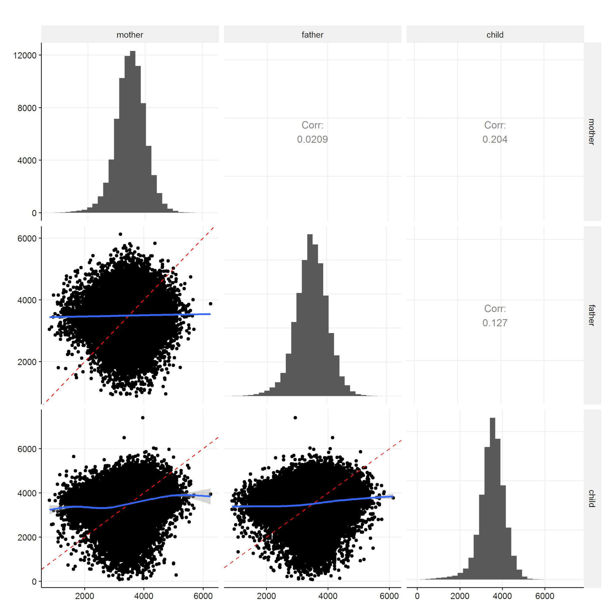
Figure 1: Birth weights (gram) for $81,144$ mother–father–child trios from the Norwegian Birth Registry. Diagonal: histograms of marginal birth weights. Lower triangle: pairwise scatter plots with estimated nonparametric regression line (blue) and identity line (dashed red), where $y=x$. Upper triangle: pairwise empirical correlation.

This simple observation may suggest that the degree of heritability of birth weight can differ in the different ranges of weight; perhaps the lowest BW values are caused by “rouge” environmental factors that act more strongly than genetic effects in the tail, or maybe they are caused by rare, recessive genes that only occasionally excert a strong negative influence on BW.

These observations motivate us to look for differences in heritability across the range of the trait value $Y$. The existing methods for investigating such differences are almost exclusively based on regression methods. In their seminal work (DeFries and Fulker, , 1985), DeFries and Fulker evaluate the degree of regression to the mean for co-twins of probands from strata in the tails of a continuous trait distribution. The idea is that if the trait is heritable, then we should observe DZ co-twins with a higher degree of regression to the mean compared to the MZ co-twins. This approach is known as DeFries-Fulker (DF) extremes analysis for twins. Later, a formal test was developed to examine whether the heritability of the trait for probands in the selected strata was equal or different to the unselected population (DeFries and Fulker, , 1988). This methodology was extended by Cherny et al. (Cherny et al., 1992a, ) by considering interaction effects between the heritability of the trait and the realized value of the trait for the proband. This approach can be used to detect linear and quadratic changes in heritability as the trait value changes. These methods all have the drawback of only providing a rough description of how the heritability varies with the trait value. The DF approach requires the researcher to select a cut-off point (a low or high trait value) for choosing the strata; the result can thus be misleading if the heritability changes smoothly as the trait value vary. Conversely, if there exists a point in the trait distribution where the heritability jumps and then stabilize again, the Cherny approach will only model this change by a linear or quadratic curve.

These drawbacks were addressed in  (Logan et al., 2012a, ) using quantile regression; by using the extended DF extremes analysis  (LaBuda et al., , 1986) as the quantile regression equation, the authors obtain a heritability measure for each quantile of the trait distribution. Consequently, their method results in a heritability measure for each value of the trait $Y=y$, corresponding to a specific quantile of the distribution.

However, in the present paper we introduce an approach based on localizing traditional genetic models. Informally, this means making sense of estimating, for instance, the additive genetic effect as a function of the phenotype; i.e. to define meaningfully $a^{2}(y)$ as the proportion of phenotype variance explained by additive genetic effects, conditional on $Y=y$. Such a definition may seem self-contradictory since one conditions on the variable whose variance is being decomposed. Nevertheless, it is fully possible to make sense of this concept, and we show in this paper how to develop heritability curves, such as $a^{2}(y)$. This definition thus provides a “local” measure of heritability, depending on the phenotype value.

As for the ACE twin model, all standard biometrical models rely on the phenotype correlations between family individuals to estimate the variance components that determine heritability. Our starting point for developing a local measure of heritability is thus a local measure of dependence between family members; more specifically, we need a local measure of correlation. There are several local measures proposed in the literature, such as the local Gaussian correlation  (Tjøstheim and Hufthammer, , 2013), the dependence function  (Holland and Wang, , 1987), and the correlation curve  (Bjerve and Doksum, , 1993). We base our approach on the correlation curve  (Bjerve and Doksum, , 1993) $\rho(y)$, which can be defined as a measure of locally explained variance, and thus fits the framework of heritability as a proportion of explained variance. The correlation curve is similar to the traditional Pearson’s correlation in that it takes values between minus one and one, and the square $\rho^{2}(y)$ is a measure of locally explained variance. In a bivariate Gaussian distribution, the correlation curve is constant (independent of $y$), and equal to the standard Pearson correlation. In contrast to the Pearson correlation the local correlation of a bivariate relationship depends on direction; for a bivariate random variable $(Y_{1},Y_{2})$, the locally explained variance of $Y_{2}$ conditional on $Y_{1}=y$ may differ from the locally explained variance of $Y_{1}$ conditional on $Y_{2}=y$.

With phenotype measurements on, for instance, a mother ($Y_{1}$) and her child ($Y_{2}$), it may seem reasonable, for instance, to study the distribution of a child phenotype conditionally on the maternal phenotype. However, most biometrical models are formulated in terms of genetic and environmental factors shared by the two family members, thus assuming a form of exchangeability between the two. This is particularly clear in twin pairs, where conditioning one twin on the other twin is unnatural. In the model of  (Logan et al., 2012b, ) this assignment was done randomly, while  (Cherny et al., 1992b, ) explored both a random assignment and a double-entry approach. However, the population value of the correlation curve can be derived from the joint distribution of two variables. If the joint distribution is exchangeable, so that $(Y_{1},Y_{2})$ has the same bivariate distribution as $(Y_{2},Y_{1})$, the correlation curve is invariant to which variable we condition on, i.e. whether we measure the locally explained variance of $Y_{1}$ conditional on $Y_{2}$ or vice versa. This means that the role of the mother and child in the above interpretation can be interchanged.

The correlation curve may be estimated parametrically or non-parametrically from observed values of a bivariate distribution $(Y_{1},Y_{2})$ by conditioning on either $Y_{1}=y$ or $Y_{2}=y$. However, our approach is instead to first model the bivariate distribution as a Gaussian mixture distribution, where the mixture distribution is restricted in such a way as to be exchangeable. From the mixture distribution, the correlation curve can be derived explicitly. We estimate the distribution by maximum likelihood, and by allowing a sufficient number of components, a mixture distribution is very flexible and fits a wide range of distributional shapes. Having obtained the parameters of the mixture distribution, the correlation curve can be derived from its explicit expression by plugging in the estimated parameters.

The paper is structured as follows. In Section 2, we define a standard mixed-effect model for continuous traits, and structure it for two specific family models: twin pairs and mother–father–child trios. Following a standard twin approach (Falconer, , 1960), and models for family trios (Magnus et al., , 2001; Lunde et al., , 2007), we derive expressions for the heritability estimates in both family structures. In Subsections 2.2 and 2.3, we explain the concept of correlation curves, and extend the traditional definition of heritability to the heritability curve, which depends on the trait value $y$. In Section 3, we introduce and analyze a Gaussian mixture (McLachlan and Peel, , 2000) for bivariate phenotype distributions, parameterized to be exchangeable. We then study the limiting behaviour of the correlation curve for large and small phenotype values under this model in Subsection 3.1. Lastly, in Subsection 3.2, we discuss the estimation of the correlation curve for the twin-pairs and the mother–father–child trios models. Section 4 provides two applications of this approach. Namely, the first application is the analysis of BMI values for twin pairs collected in the dataset “twinData”, found in the R-package ”OpenMx” (Neale et al., , 2016); the second one is the analysis of birth weight data of mother–father–child trios from the Medical Birth Registry of Norway. For both family structures we compute AIC and BIC values to select the best-fitting mixture models, and explore the resulting distributions and heritability curves. Proofs are provided in an appendix.

2 Development of Heritability curves

2.1 Traditional models for twins and family trios

We first provide a basic description of how traditional biometrical models can be set up in some generality, and in particular for twins and family trios. While there are numerous ways of building, parametrizing, and interpreting such models, our approach is fairly standard, and in a form that supports our development of heritability curves. Let $Y_{ij}$ be the trait value of individual $j$ in a family $i$, and consider the mixed-effect model (see e.g.  (McCulloch and Neuhaus, , 2001))

$$Y_{ij}=\mu+\beta^{t}x_{ij}+A_{ij}+C_{ij}+D_{ij}+E_{ij},$$ (2.1)

where $A_{ij}$, $C_{ij}$, $D_{ij}$ and $E_{ij}$ represent additive genetic, common environmental, dominant genetic, and residual environmental random effects, respectively (see e.g.  (Falconer, , 1960)). We assume the four components $A_{ij}$, $C_{ij}$, $D_{ij}$ and $E_{ij}$ to be mutually independent, with mean $0$ and variances $\sigma_{A}^{2}$, $\sigma_{C}^{2}$, $\sigma_{D}^{2}$ and $\sigma_{E}^{2}$. The inclusion of the term $\beta^{t}x_{ij}$ (fixed effects) allows the average phenotype level to depend on covariates. Note that this model assumes no gene-environment interaction. In traditional biometrical modelling (see e.g.  (Gjessing and Lie, , 2008)) the random effects are assumed to be normally distributed with expectation $0$, i.e. $A_{ij}\sim N(0,\sigma_{A}^{2})$, $C_{ij}\sim N(0,\sigma_{C}^{2})$, $D_{ij}\sim N(0,\sigma_{D}^{2})$ and $E_{ij}\sim N(0,\sigma_{E}^{2})$. The assumption of normality is seen as natural based on the central limit theorem if $Y$ is the result of numerous small, independent genetic and environmental effects that add up to produce the trait value. Under the above assumptions the total variance of the trait is given by

$$\sigma^{2}=Var(Y_{ij})=\sigma_{A}^{2}+\sigma_{C}^{2}+\sigma_{D}^{2}+\sigma_{E}^{2}.$$ (2.2)

We define $a^{2}=\sigma_{A}^{2}/\sigma^{2}$, $c^{2}=\sigma_{C}^{2}/\sigma^{2}$, $d^{2}=\sigma_{D}^{2}/\sigma^{2}$, and $e^{2}=\sigma_{E}^{2}/\sigma^{2}$ as the proportions of the total variance that derive from each of the four genetic and environmental components. Note that

$$a^{2}+c^{2}+d^{2}+e^{2}=1,$$

i.e. the contributions from all components sum to one. Thus, in a model including $A$, $C$, and $E$, excluding dominant effects, one may quantify the genes-versus-environment contribution to trait variability as $a^{2}$. This proportion is often referred to as heritability and can be interpreted as how strongly the genetic effect $A_{ij}$ contributes to the trait value. The heritability based on the additive genetic component is often referred to as narrow sense heritability. Some models may also include dominant genetic effects, and in such cases one may refer to $a^{2}+d^{2}$ as the broad sense heritability (Khoury et al., , 1993).

From independent observations of $Y_{ij}$ alone, it is not possible to identify the individual variance components $\sigma_{A}^{2}$, $\sigma_{C}^{2}$, $\sigma_{D}^{2}$, and $\sigma_{E}^{2}$ in (2.2), only the total variance $\sigma^{2}$. In order to make the individual variances identifiable, one has to consider data on family members, for which the $Y$’s are correlated due to shared genetic material and environment. We focus on two basic family structures — mother–father–child trios and twin pairs — in the following. As is well known, these family structures are quite restricted in the number of effects they allow to be estimated, and assumptions have to be made about what genetic and environmental effects to include in each model. In the following, we will present the specific models that will serve as illustrations when developing heritability curves.

2.1.1 Twins

Perhaps the best known biometrical model is the ACE model for twins, complemented by the alternative ADE model. While the expressions for twin correlations in these models are very well known, we state them here as a starting point for the heritability curves.

Let $Y_{ij}$ be the trait value of twin $j$ ($j=1,2$) in twin-pair $i$. Let $\rho^{(MZ)}$ and $\rho^{(DZ)}$ be the phenotype correlations $\operatorname{cor}(Y_{i1},Y_{i2})$ for MZ and DZ twins, respectively. Both ACE and ADE models include the additive genetic component $A$. For MZ-twins $\operatorname{cor}(A_{i1},A_{i2})=1$, while for DZ-twins $\operatorname{cor}(A_{i1},A_{i2})=1/2$. In the standard ACE model, the correlation for the common environmental effect is assumed to be $\operatorname{cor}(C_{i1},C_{i2})=1$ in all twin pairs; thus, one makes the common assumption of DZ twins sharing their environment to the same degree as the MZ twins. In the alternative ADE one assumes $\operatorname{cor}(D_{i1},D_{i2})=1$ for MZ twins and $\operatorname{cor}(D_{i1},D_{i2})=1/4$ for DZ twins. In both models, residual environmental effects are assumed to be independent.

Since the basic twin models utilize only the $\rho^{(MZ)}$ and $\rho^{(DZ)}$ phenotype correlations, they allow estimating two parameters. In addition, $e{{}^{2}}$ can be estimated from $e^{2}=1-a^{2}-c^{2}-d^{2}$. The ACE model assumes $d^{2}=0$, and thus the parameters $a^{2}$, $c^{2}$, and $e^{2}$ can be identified; the ADE model assumes $c^{2}=0$, and thus the parameters $a^{2}$, $d^{2}$, and $e^{2}$ can be identified.

For the ACE model, it follows from the above that

$$\rho^{(MZ)} = a^{2}+c^{2},$$

$$\rho^{(DZ)} = \frac{1}{2}a^{2}+c^{2}.$$

For the ADE model, the equations are

$$\rho^{(MZ)} =a^{2}+d^{2},$$

$$\rho^{(DZ)} =\frac{1}{2}a^{2}+\frac{1}{4}d^{2}.$$

The simplest approach to estimating $a^{2}$, $c^{2}$, and $d^{2}$ is by moment estimators, i.e. to solve this set of equations, using empirical values for $\rho^{(MZ)}$ and $\rho^{(DZ)}$, and use $e^{2}=1-a^{2}-c^{2}-d^{2}$ to estimate $e^{2}$. The resulting solutions for the ACE model are the celebrated formulas of Falconer: (Falconer, , 1960)

$$a^{2}=2(\rho^{(MZ)}-\rho^{(DZ)}),$$

$$c^{2}=2\rho^{(DZ)}-\rho^{(MZ)},$$ (2.3)

$$e^{2}=1-\rho^{(MZ)}.$$

For the ADE model, the corresponding set of solutions are

$$a^{2} =4\rho^{(DZ)}-\rho^{(MZ)},$$

$$d^{2} =2(\rho^{(MZ)}-2\rho^{(DZ)}),$$ (2.4)

$$e^{2} =1-\rho^{(MZ)}.$$

Without further assumptions, an informal choice between the ACE and ADE models is often made based on whether empirically $\rho^{(MZ)}<2\rho^{(DZ)}$ or not. If this is the case, the ACE model is a natural choice; otherwise, the ADE model can be used.

2.1.2 Mother-father-child trios

Let $Y_{ij}$ be the observed trait value of individual $j$ in nuclear family trio $i$. We let $j=1,2,3$ correspond to the mother, father, and child, respectively. A phenotype correlation between mother and father may signify, for instance, assortative mating, inbreeding, or social homogamy among the parents. However, the correlation is typically low, and we will here assume it is zero (Magnus et al., , 2001). There are thus only two correlations that provide information: the mother-child and father-child correlations. There are numerous ways of parametrizing correlations in nuclear families (Magnus et al., , 2001; Pawitan et al., , 2004; Lunde et al., , 2007; Gjessing and Lie, , 2008; Rabe-Hesketh et al., , 2008), but being restricted to two correlations means that these cannot be separated. In our setting, we assume, for additive autosomal genes, that $\operatorname{cor}(A_{i1},A_{i3})=\operatorname{cor}(A_{i2},A_{i3})=1/2$, and that $\operatorname{cor}(A_{i1}A_{i2})=0$ for the parents. Also, we assume that mother and child share an environmental component, but no such sharing between father and child, leading to $\operatorname{cor}(C_{i1},C_{i3})=1$ and $\operatorname{cor}(C_{i2},C_{i3})=0$. Thus,

$$\Sigma_{A}=\sigma_{A}^{2}\begin{bmatrix}1&0&1/2\\ 0&1&1/2\\ 1/2&1/2&1\end{bmatrix},\quad\Sigma_{C}=\sigma_{C}^{2}\begin{bmatrix}1&0&1\\ 0&1&0\\ 1&0&1\end{bmatrix},\textrm{ and }\Sigma_{E}=\sigma_{E}^{2}\begin{bmatrix}1&0&0\\ 0&1&0\\ 0&0&1\end{bmatrix}$$

are the covariance matrices for the vectors $(A_{i1},A_{i2},A_{i3})$, $(C_{i1},C_{i2},C_{i3})$, and $(E_{i1},E_{i2},E_{i3})$, respectively.

A graphical representation of the above model is displayed in a path diagram in Figure 2.

Under the above assumptions the vectors $(Y_{i1},Y_{i2},Y_{i3})$ are i.i.d. multivariate normal with mean

$$(\mu+\beta^{t}x_{i1},\mu+\beta^{t}x_{i2},\mu+\beta^{t}x_{i3})$$ (2.5)

and covariance matrix

$$\Sigma=\Sigma_{A}+\Sigma_{C}+\Sigma_{E}=(\sigma_{A}^{2}+\sigma_{C}^{2}+\sigma_{E}^{2})\begin{bmatrix}1&0&\frac{1}{2}a^{2}+c^{2}\\ 0&1&\frac{1}{2}a^{2}\\ \frac{1}{2}a^{2}+c^{2}&\frac{1}{2}a^{2}&1\end{bmatrix},$$ (2.6)

where $a^{2}$, $c^{2}$, and $e^{2}$ are defined as above. Again, the unknown values can simply be estimated by the methods of moments by matching the correlation matrix (2.6) to its empirical counterpart, and solve for $a^{2}$, $c^{2}$ and $e^{2}$ under the constraint $a^{2}+c^{2}+e^{2}=1$. The solution is given by the following equations

$$a^{2} = 2\rho^{(FC)}$$

$$c^{2} = \rho^{(MC)}-\rho^{(FC)}$$ (2.7)

$$e^{2} = 1-\rho^{(MC)}-\rho^{(FC)},$$

where $\rho^{(MC)}$ and $\rho^{(FC)}$ are the mother-child and father-child correlations, respectively.

We will, in the following, use these solutions, and those for the ADE twin model, to obtain local versions of $a^{2}$, $c^{2}$, $d^{2}$, and $e^{2}$. Note that in both cases, the underlying assumption is that the covariance (correlation) matrix completely characterizes the dependence structure between traits in a family and can be decomposed as in e.g. (2.6).

Figure 2: Path diagram representing the birth weight of mother $Y_{1}$, father $Y_{2}$, and child $Y_{3}$ (represented as squares). The traits are determined by the unobserved genotype values ($A$) and environmental values ($C$) (shown as circles), as well as the independent residual environmental values ($E$) (not shown).

2.2 Correlation curves for non-linear bivariate relationships

We now explain the concept of local correlation curves, following the approach of Bjerve and Doksum (Bjerve and Doksum, , 1993). To illustrate the principle of localization, we use simulated data from a hypothetical phenotype, as seen in Figure 3(a).

We consider two strata (A and B) consisting of all mother-child pairs for which the mother’s trait $Y_{1}=y_{1}$ falls within two intervals (interval A and B) on the x-axis. The corresponding correlation curve is shown in Figure 3(b); as a function of $y_{1}$ (horizontal axis) it is smaller in stratum A than in stratum B. This indicates that the mother-child association is stronger in stratum B compared to stratum A. In a non-parametric regression setting, this would mean that the child’s trait can be predicted by the mother’s trait with higher precision in stratum B than in stratum A. For both strata, an increase in the mother’s trait is associated with an increase in the child’s trait since the correlation curve is positive. Since the correlation curve is continuous, the location argument $y_{1}$ can be seen as the center of infinitesimal intervals from which strata such as A and B can be constructed, while the value of the correlation curve is a measure of dependence for the corresponding strata. A constant correlation curve indicates that the dependence properties are constant across these strata, while a varying correlation curve indicates strata that differ in their dependence properties.

Figure 3: Illustration of the concept of a correlation curve and the role of exchangeability using simulated data. Strata A and B include all mother-child pairs for which the mother’s trait value falls in the intervals $[1,2]$ and $[9,10]$, respectively. Strata $A^{*}$ and $B^{*}$ include all mother-child pairs for which the child’s trait value falls in the same intervals.

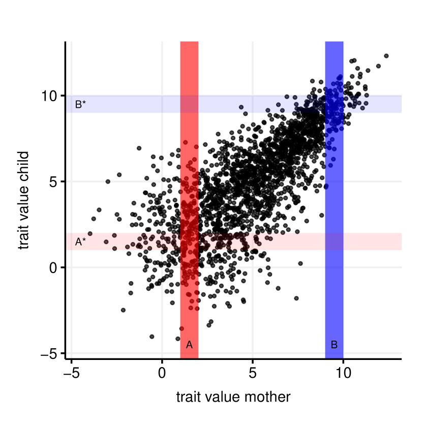
(a) Simulated data from an exchangeable Gaussian mixture, and the definition of strata.

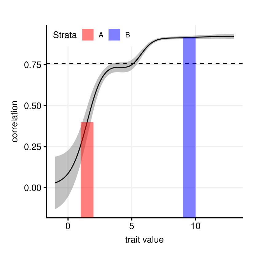
(b) Estimated correlation curve for the data displayed in panel (a), and 95% pointwise confidence intervals are shown in grey. The height of the bars displays the average value of the correlation curve within strata $A$ and $B$.

If the joint distribution is exchangeable, so that $(Y_{1},Y_{2})$ has the same bivariate distribution as $(Y_{2},Y_{1})$, the correlation curve is invariant to which variable we condition on, i.e. whether we measure the locally explained variance of $Y_{1}$ conditional on $Y_{2}$ or vice versa. This means that the role of the mother and child in the above interpretation can be interchanged, and the dependence structure in strata $A^{*}$ and $B^{*}$ in Figure 3(a)) is similar to the dependence structure in strata $A$ and $B$; the correlation curve $\rho(y)$ as a function of $y$ thus represents a measure of the mother-child trait dependence when either the mother or the child has trait value equal to $y$. In the next section, we show more precisely how $\rho(y)$ is defined in terms of locally explained variance.

2.2.1 Standard correlation curves for bivariate relationships

Let $(Y_{1},Y_{2})$ be random variables from a bivariate continuous distribution, and define $\tau_{1}^{2}=\operatorname{Var}(Y_{1})$, $\tau_{2}^{2}=\operatorname{Var}(Y_{2})$, and $\rho=\operatorname{cor}(Y_{1},Y_{2})$. Further, define $\mu(y)=\operatorname{E}(Y_{1}|Y_{2}=y)$ and $\sigma^{2}(y)=\operatorname{Var}(Y_{1}|Y_{2}=y)$ as functions of $y$. Assuming that $\mu(y)$ is differentiable, define $\beta(y)=\mu^{\prime}(y)$, i.e. the slope of the (typically non-linear) regression curve $\mu(y)$ when $Y_{1}$ is regressed on $Y_{2}$. Recall that in a standard linear regression context, $\mu(y)$ is a linear function of $y$, where the slope $\beta_{1|2}:=\beta(y)$ and the conditional variance $\sigma_{1|2}^{2}:=\sigma^{2}(y)$ are both constant.

By the law of total variance,

$$\operatorname{Var}(Y_{1})=\operatorname{Var}(\operatorname{E}(Y_{1}|Y_{2}))+\operatorname{E}(\operatorname{Var}(Y_{1}|Y_{2})),$$

and it thus seems natural to define in general

$$\text{Proportion of }\operatorname{Var}(Y_{1})\text{ explained by }Y_{2}=\frac{\operatorname{Var}(\operatorname{E}(Y_{1}|Y_{2}))}{\operatorname{Var}(\operatorname{E}(Y_{1}|Y_{2}))+\operatorname{E}(\operatorname{Var}(Y_{1}|Y_{2}))}.$$

In the case of linear regression, $\operatorname{Var}(\operatorname{E}(Y_{1}|Y_{2}))=\tau_{2}^{2}\beta_{1|2}^{2}$ and $\operatorname{E}(\operatorname{Var}(Y_{1}|Y_{2}))=\sigma_{1|2}^{2}$, and the proportion of explained variance can thus be written

$$\frac{(\tau_{2}\beta_{1|2})^{2}}{(\tau_{2}\beta_{1|2})^{2}+\sigma_{1|2}^{2}}=\left(\frac{\tau_{2}\beta_{1|2}}{\tau_{1}}\right)^{2}=\rho^{2},$$ (2.8)

which is the usual formula for explained variance in a linear regression.

We want to define a “local” variant of $\rho^{2}$, describing the proportion of explained variance when $Y_{2}=y$, thus to define $\rho^{2}(y)$ as a function of $y$. To this end, (2.8) is a natural starting point, and the extension to a non-linear setting would thus be to allow both $\beta(y)$ and $\sigma^{2}(y)$ to depend on $y$. This leads to the definition

$$\rho(y)=\frac{\tau_{2}\beta(y)}{\left[\left(\tau_{2}\beta(y)\right)^{2}+\sigma^{2}(y)\right]^{1/2}},$$ (2.9)

where we recall that $\tau_{2}^{2}=\operatorname{Var}(Y_{2})$, $\beta(y)=\frac{d}{dy}\,\operatorname{E}(Y_{1}|Y_{2}=y)$, and $\sigma^{2}(y)=\operatorname{Var}(Y_{1}\mid Y_{2}=y)$.

Indeed, this is the formula developed by Bjerve et al. (Bjerve and Doksum, , 1993) and Doksum et al. (Doksum et al., , 1994). As pointed out by Bjerve et al., the correlation curve should not be confused with the conditional correlation obtained by applying the usual correlation formula to the conditional distribution of $(Y_{1},Y_{2})$ given $Y_{2}=y$, which would always be zero. It should also be noted that while $\tau_{2}$ is kept fixed in (2.9), the denominator $\left(\tau_{2}\beta(y)\right)^{2}+\sigma^{2}(y)$ is no longer necessarily equal to $\tau_{1}^{2}=\operatorname{Var}(Y_{1})$ from the original distribution. In fact, for a fixed $y=y_{0}$, it corresponds to $\operatorname{Var}(Z_{1})$ from a hypothetical bivariate distribution $(Z_{1},Z_{2})$ where $\operatorname{Var}(Z_{2})=\tau_{2}^{2}$ and $\operatorname{Var}(Z_{1})$ is determined from having a linear regression of $Z_{1}$ on $Z_{2}$ with constant slope $\beta(y_{0})$ and constant conditional variance $\operatorname{Var}(Z_{1}|Z_{2})=\sigma^{2}(y_{0})$.

2.2.2 Correlation curves for symmetric bivariate relationships

In our setting, we are interested in relationships between pairs of family members, for example, a pair of twins or a child and a parent. We denote the pair’s respective trait values by $Y_{1}$ and $Y_{2}$. At first glance, it may seem natural to ask about the explained variation of a child trait $Y_{1}$, conditional on its parental value $Y_{2}$. However, this is less natural for twins, who are from the same generation. Indeed, most biometrical models assume that the positive correlation between the trait values is generated by shared genes and shared environment; the sharing is symmetrical between family members, and the generational aspect is only used to compute the degree of relatedness. That is, in pairs of family members, the two members should be exchangeable, so that $(Y_{1},Y_{2})$ and $(Y_{2},Y_{1})$ have the same bivariate distribution. Clearly, this means that when applying (2.9) in a heritability setting, it would be reasonable to expect that $Y_{1}$ conditional on $Y_{2}$ should provide the same answers as $Y_{2}$ conditional on $Y_{1}$. While exchangeability is obviously not the case for general bivariate distributions, we achieve pairwise exchangeability by a corresponding restriction of our parametric models for the bivariate distributions, as described later. When including covariates, the assumption of pairwise exchangeability should apply to the residuals, i.e. the mean-adjusted traits $Y_{1}-\beta^{t}x_{1}$ and $Y_{2}-\beta^{t}x_{2}$.

Note that it would suffice to assume that, for all $y$,

$$\tau_{1}^{2}=\operatorname{Var}(Y_{1}) =\operatorname{Var}(Y_{2})=\tau_{2}^{2}=:\sigma,$$

$$\operatorname{E}(Y_{1}\mid Y_{2}=y) =\operatorname{E}(Y_{2}\mid Y_{1}=y)=:\mu(y),$$ (2.10)

$$\operatorname{Var}(Y_{2}\mid Y_{1}=y) =\operatorname{Var}(Y_{1}\mid Y_{2}=y)=:\sigma^{2}(y),$$

since this would imply that (2.9) would be invariant to the direction of conditioning. However, the models presented in this paper all imply full pairwise exchangeability. We do not, however, ask for full exchangeability of the multivariate outcome distribution; for instance, a mother-father-child trio would clearly not have the same trivariate distribution as a child-father-mother trio. Nevertheless, the pairwise exchangeability implies that all family members have the same marginal distributions. The appropriateness of the exchangeability assumptions will be addressed in the Discussion.

2.3 Heritability curves

Assuming $\rho(y)$ to be well defined for the joint distribution of the two family members, we are interested in the degree to which the value of $\rho(y)$ can be attributed to heritability on one side, and to environment on the other. In particular, we are interested in knowing how these contributions vary with $y$.

Definition 1 (Heritability curve for the twin ADE model).

Assume the exchangeability property (2.2.2) holds for both MZ and DZ bivariate distributions. Adopting the moment equations (2.1.1), we define the heritability curve by

$$a^{2}(y)=4\rho^{(DZ)}(y)-\rho^{(MZ)}(y),$$ (2.11)

where $\rho^{(MZ)}(y)$ and $\rho^{(DZ)}(y)$ are the correlation curves of MZ and DZ twins calculated according to (2.9). Similarly, (2.1.1) allows local versions of the dominance effect

$$d^{2}(y)=2\left[(\rho^{(MZ)}(y)-2\rho^{(DZ)}(y)\right]$$ (2.12)

and residual environment

$$e^{2}(y)=1-\rho^{(MZ)}(y)$$ (2.13)

to be defined.

Note that with Equation (2.11), a trait value can in principle display a non-linear association within both MZ and DZ twins, but have constant local heritability $a^{2}(y)$ due to a canceling effect in $4\rho^{(DZ)}(y)-\rho^{(MZ)}(y)$.

We similarly define the heritability curve for family trios by adopting the genetic model described in Section 2.1.2 locally.

Definition 2 (Heritability curve for an ACE model of mother-father-child trios).

Assuming the exchangeability property (2.2.2), let $\rho^{(MC)}(y)$ and $\rho^{(FC)}(y)$ be correlation curves (2.9) for mother-child and father-child relationships, respectively. The heritability curves $a^{2}(y)$, $c^{2}(y)$, and $e^{2}(y)$ are then given by

$$a^{2}(y) =2\rho^{(FC)}(y)$$ (2.14)

$$c^{2}(y) =\rho^{(MC)}(y)-\rho^{(FC)}(y)$$ (2.15)

$$e^{2}(y) =1-\rho^{(MC)}(y)-\rho^{(FC)}(y)$$ (2.16)

We next define a parametric class of multivariate densities for family data that can easily be fit by maximum likelihood, allows for non-linear dependence, and admits an analytical expression for the correlation curve (2.9).

3 Correlation and heritability curves for Gaussian mixtures

Throughout this paper we denote by $\phi_{d}\!\left(\boldsymbol{y};\boldsymbol{\mu},\boldsymbol{\Sigma}\right)$ a $d$ dimensional Gaussian density, evaluated at $\boldsymbol{y}=(y_{1},\ldots,y_{d})$, and with mean vector $\boldsymbol{\mu}$ and covariance matrix $\boldsymbol{\Sigma}$. We will only use $d=1,2,3$.

Consider the observed trait vector $\boldsymbol{y}=(y_{1},y_{2})$ for a pair of family members. We assume that it follows a $m$-component Gaussian mixture with density

$$\sum_{k=1}^{m}p_{k}\phi_{2}\!\left(\boldsymbol{y};\boldsymbol{\mu}_{k},\boldsymbol{\Sigma}_{k}\right),$$ (3.1)

where $\sum_{k=1}^{m}p_{k}=1$. The mean and covariance structure of the the $k$th mixture component is taken to be

$$\boldsymbol{\mu}_{k}=(\mu_{k},\mu_{k}),\quad\boldsymbol{\Sigma}_{k}=\begin{pmatrix}\sigma_{k}^{2}&\sigma_{k}^{2}\rho_{k}\\ \sigma_{k}^{2}\rho_{k}&\sigma_{k}^{2}\end{pmatrix},$$ (3.2)

where $\rho_{k}\in(-1,1)$ is the correlation parameter. The components of the mixture are ordered such that $\sigma_{1}\leq\dots\leq\sigma_{m}$. If $\sigma_{q}=\sigma_{q+1}=\dots=\sigma_{m}$ for some $q<m$, then we order the components in ascending order with respect of the means, i.e. $\mu_{q}<\dots<\mu_{m}$. Note that under the above constraints on $\boldsymbol{\mu}_{k}$ and $\boldsymbol{\Sigma}_{k}$, the exchangeability condition (2.2.2) is satisfied. In addition, $Y_{1}$ and $Y_{2}$ have the same marginal distribution, with marginal density

$$g(y)=\sum_{k=1}^{m}g_{k}(y)$$ (3.3)

as the sum over the individual (weighted) components $g_{k}(y):=p_{k}\phi_{1}\!\left(y;\mu_{k},\sigma_{k}^{2}\right)$. The (total) marginal mean, marginal variance, and correlation are given by

$$\mu=\sum_{k=1}^{m}p_{k}\mu_{k},\quad\sigma^{2}=\sum_{k=1}^{m}p_{k}\left[\sigma_{k}^{2}+(\mu_{k}-\mu)^{2}\right]\quad\text{and}\quad\rho=\sigma^{-2}\sum_{k=1}^{m}p_{k}\left[\rho_{k}\sigma_{k}^{2}+(\mu_{k}-\mu)^{2}\right].$$ (3.4)

We next derive local versions of $\mu$ and $\sigma$. Let $\delta$ be a latent variable with $P(\delta=k)=p_{k}$, $k=1,\dots m$, showing which mixture component is realized. From Bayes’ rule, it follows that the distribution of $\delta\mid Y_{2}=y$ is given as

$$p_{k}^{*}(y):=P(\delta=k\mid Y_{2}=y) =\frac{g_{k}(y)}{g(y)}.$$ (3.5)

Also, by the assumed normality of each mixture component, it follows that

$$\mu_{k}(y):=\operatorname{E}(Y_{1}\mid Y_{2}=y,\delta=k)=\mu_{k}+\rho_{k}\cdot(y-\mu_{k}),$$

i.e. $\mu_{k}(y)$ is a line with slope $\rho_{k}$, going through the point $(\mu_{k},\mu_{k})$. By the law of total expectation,

$$\begin{split}\mu(y)&:=\operatorname{E}(Y_{1}|Y_{2}=y)=\operatorname{E}\left[\operatorname{E}\left(Y_{1}\mid Y_{2}=y,\delta\right)\mid Y_{2}=y\right]\\ &=\sum_{k=1}^{m}p_{k}^{*}(y)\mu_{k}(y).\end{split}$$ (3.6)

Similarly, by the law of total variance:

$$\begin{split}\sigma^{2}(y)&:=\operatorname{Var}(Y_{1}|Y_{2}=y)\\ &=\operatorname{E}\left[\operatorname{Var}\left(Y_{1}\mid Y_{2}=y,\delta=k\right)\mid Y_{2}=y\right]\\ &\phantom{=}+\operatorname{Var}\left[\operatorname{E}\left(Y_{1}\mid Y_{2}=y,\delta=k\right)\mid Y_{2}=y\right]\\ &=\operatorname{E}\left(\sigma_{\delta}^{2}(1-\rho_{\delta}^{2})\mid Y_{2}=y\right)+\operatorname{Var}\left(\mu_{\delta}(y)\mid Y_{2}=y\right)\\ &=\sum_{k=1}^{m}p_{k}^{*}(y)\left[\sigma_{k}^{2}(1-\rho_{k}^{2})+\left[\mu_{k}(y)-\mu(y)\right]^{2}\right].\end{split}$$ (3.7)

We are now ready to give the expression for $\beta(y)=\mu^{\prime}(y)$, to be used in the correlation curve (2.9) for the mixture distribution.

Proposition 1.

Define

$$d_{k}(y):=-(y-\mu_{k})/\sigma_{k}^{2}.$$

Then,

$$\beta(y)= \sum_{k=1}^{m}p_{k}^{*}(y)\left[\rho_{k}+\left(\mu_{k}(y)-\mu(y)\right)d_{k}(y)\right],$$ (3.8)

where $p_{k}^{*}(y)$ is given by (3.5).

Proof.

See Appendix. ∎

Notice that when there is only a single mixture component $(m=1)$, yielding a bivariate Gaussian distribution, the above expressions reduce to $\sigma=\sigma_{1}$, $\mu(y)=\mu_{1}$, $\sigma^{2}(y)=\sigma^{2}_{1}(1-\rho^{2}_{1})$ and $\beta(y)=\rho_{1}$. Inserting these expressions in (2.9) we get a constant correlation curve, $\rho(y)=\rho_{1}$ for every $y$. Hence, if $m=1$ the heritability curve $a^{2}(y)$, given by (2.11) or (2.14), reduces to the ordinary heritability coefficient $a^{2}$.

3.1 Properties of the correlation curve under a Gaussian mixture

It is of interest to investigate the asymptotic behaviour of $\rho(y)$ as $y\rightarrow\pm\infty$ under the mixture (3.1) since this can be used to evaluate the asymptotic behaviour of the heritability curve $a^{2}(y)$, which in general will depend on the family design. We state the result in the following theorem, which also includes the limit behaviour of $\beta(y)$ and $\sigma^{2}(y)$.

Intuitively, a one-dimensional mixture distribution is asymptotically dominated in the tails by the component with the largest variance; if two or more components all share the largest variance, the sizes of the mean values come into play, with the component with the smallest mean value dominating when $y\to-\infty$, and the largest when $y\to+\infty.$ While this in itself is fairly obvious, we here use it to develop the resulting asymptotic behavior of $\beta(y)$, $\sigma^{2}(y)$, and $\rho(y)$.

We consider the following two cases: Recall the ordering $\sigma_{1}^{2}\leq\cdots\leq\sigma_{m}^{2}$, and define $q=\min\left\{l:\sigma_{l}^{2}=\sigma_{m}^{2}\right\}$. We define Case I as $q=m$. For the alternative, Case II, where $q<m$, our conventions is that the mean values are then ordered such that $\mu_{q}<\mu_{m}$. To simplify the notation, define the constant $K$ as follows:

$$\begin{array}[]{ccc}\text{Case I }(q=m),&y\to\pm\infty,&K:=m,\\ \text{Case II }(q<m),&y\to-\infty,&K:=q,\\ \text{Case II }(q<m),&y\to+\infty,&K:=m.\end{array}$$

Theorem 3.1.1.

The asymptotic behavior of $\beta(y)$, $\sigma^{2}(y)$, and $\rho(y)$, given by (3.8), (3.7), and (2.9), are

$$\lim_{y}\beta(y) =\rho_{K},$$

$$\lim_{y}\sigma^{2}(y) =\sigma_{K}^{2}(1-\rho_{K}^{2}),$$

$$\lim_{y}\rho(y) =\tilde{\rho}_{K}:=\frac{\sigma\rho_{K}}{\left[\sigma^{2}\rho_{K}^{2}+\sigma_{K}^{2}(1-\rho_{K}^{2})\right]^{1/2}}.$$ (3.9)

The global variance $\sigma^{2}$ is defined as in (3.4).

Proof.

See Appendix. ∎

Theorem 3.1.1 shows that $\beta(y)$, $\sigma^{2}(y)$, and $\rho(y)$ all stabilize to finite limits as $y\rightarrow\pm\infty$, and their behaviour is determined by the variance and correlation of mixture component $K$, in addition to the global variance $\sigma^{2}$. In Case I we have that the asymptotic correlation is the same in both tails, as exemplified in Figure 4a) where $K=3$ and $\tilde{\rho}_{3}\approx 0.5$.

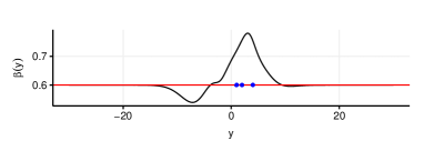
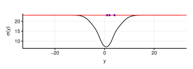
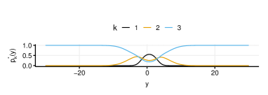
Figure 4: Illustration of the asymptotic tail behaviour (red line) of the correlation curve and its builing blocks under a $m=3$ component mixture model: (a) $\rho(y)$, (b) $\beta(y)$, (c) $\sigma^{2}(y)$, and (d) $p_{k}^{*}(y)$. The mixture model has parameters $\left(\sigma_{1},\sigma_{2},\sigma_{3}\right)=\left(2,4,6\right)$, $\left(\mu_{1},\mu_{2},\mu_{3}\right)=\left(1,2,4\right)$, $\left(\rho_{1},\rho_{2},\rho_{3}\right)=\left(0.7,0.8,0.6\right)$ and $\left(p_{1},p_{2},p_{3}\right)=(0.3,0.3,0.4)$.

Identical correlations in both tails may seem unmotivated for family data. Still, within the data range the correlation curve will be determined by all of the mixture components, in accordance with (2.9), which allows for different behaviour in the tails.

Case II, on the other hand, allows for different asymptotic correlation in the left and right tail, with the differences being the use of $\rho_{n}$ versus $\rho_{m}$ in (3.9).

Theorem 3.1.1 is further illustrated in Figure 4 showing the limiting behaviour of $\beta(y)$, $\sigma^{2}(y)$, and $\rho(y)$ for a three-component mixture under Case I. Note that the limiting correlation satisfies $\tilde{\rho}_{3}<\min(\rho_{1},\rho_{2},\rho_{3})$ for the parameter values used in the figure. This is counter-intuitive because the posterior probability $p_{3}^{*}(y)$ approaches 1 in the tails (upper left panel), but still the limiting correlation is not simply $\rho_{3}$. The peak in correlation around $\mu_{2}=2$ is reasonable as the second component has the highest $\rho$.

3.1.1 The case of equal $\sigma_{k}$’s

It is worth studying the special case that $\sigma_{1}=\sigma_{2}=\cdots=\sigma_{m}$, with their common value denoted by $\sigma_{0}$. This is Case II of Theorem 3.1.1 with $q=1$. From (3.4) we get $\sigma^{2}=\sigma_{0}^{2}+\sigma_{\mu}^{2}$, where

$$\sigma_{\mu}^{2}=\sum_{k=1}^{m}p_{k}(\mu_{k}-\mu)^{2},$$ (3.10)

which is the variance due to differences in locations of mixture components. Recall the convention that the mixture components are ordered such that $\mu_{1}<\mu_{2}<\cdots<\mu_{m}$. We are now ready to state the following corollary to Theorem 3.1.1.

Corollary 3.1.2.

When $\sigma_{1}=\cdots=\sigma_{m}$ the asymptotic behavior of $\rho(y)$, given by (2.9), is

$$\lim_{y\rightarrow-\infty}\rho(y)=\rho_{1}\sqrt{\frac{1+\gamma}{1+\gamma\rho_{1}^{2}}}\quad\hbox{and}\quad\lim_{y\rightarrow\infty}\rho(y)=\rho_{m}\sqrt{\frac{1+\gamma}{1+\gamma\rho_{m}^{2}}},$$ (3.11)

where $\gamma=\sigma_{\mu}^{2}/\sigma_{0}^{2}$ is the ratio of between and within-component variance in the Gaussian mixture.

The limiting correlations always exceed (in absolute value) $\rho_{1}$ and $\rho_{m}$, respectively. When $\gamma\rightarrow\infty$, i.e. the mixture components gets increasingly spread out, both limits approach 1 in absolute value.

3.2 Estimation

In this section we explain how to fit Gaussian mixtures to family data. On one hand, they are fully parametric distributions, which can be exploited in estimation and inference. On the other hand, allowing the number of mixture components $m$ to grow, mixtures become increasingly flexible, which allows us to view them also as nonparametric tools. In particular, Gaussian mixtures seem well suited to model small perturbations from Gaussianity.

First, let $\boldsymbol{y}=(y_{1},y_{2},y_{3})$ denote the trait vector for the mother-father-child trio, which is assumed to have the following mixture density:

$$\sum_{k=1}^{m}p_{k}\phi_{3}\!\left(\boldsymbol{y};\boldsymbol{\mu}_{k},\boldsymbol{\Sigma}_{k}\right).$$

Here $\boldsymbol{\mu_{k}}$, $\boldsymbol{\Sigma_{k}}$ are structured in the following way:

$$\boldsymbol{\mu}_{k}=(\mu_{k},\mu_{k},\mu_{k}),\quad\boldsymbol{\Sigma}_{k}=\begin{pmatrix}\sigma^{2}_{k}&\sigma^{2}_{k}\rho_{k}^{(MF)}&\sigma^{2}_{k}\rho_{k}^{(MC)}\\ \sigma^{2}_{k}\rho_{k}^{(MF)}&\sigma^{2}_{k}&\sigma^{2}\rho_{k}^{(FC)}\\ \sigma^{2}_{k}\rho_{k}^{(MC)}&\sigma^{2}_{k}\rho_{k}^{(FC)}&\sigma^{2}_{k}\end{pmatrix},$$ (3.12)

where we use superscripts on the $\rho$’s to denote relationship. Integrating the above joint density with respect to any one of the three family members ($y_{1}$, $y_{2}$, or $y_{3}$) will result in the bivariate Gaussian mixture (3.1) from which we defined the correlation curve. The reason for performing joint estimation, rather than pairwise, is to optimally utilize the information contained in mother-father-child trios. Note that the three marginals are identical by construction, although the joint distribution is not exchangeable unless $\rho_{k}^{(MF)}=\rho_{k}^{(MC)}=\rho_{k}^{(FC)}$ for $k=1,\ldots,m$.

Given $n$ such trios, the parameters ($\mu_{k}$, $\sigma_{k}$, $\rho_{k}$, $p_{k}$) can be estimated by maximizing the following log-likelihood:

$$\log L=\sum_{i=1}^{n}\log\left[\sum_{k=1}^{m}p_{k}\phi_{3}\!(\boldsymbol{y}_{i};\boldsymbol{\mu}_{k},\Sigma_{k})\right].$$ (3.13)

Once the parameters are estimated, the heritability curve $a^{2}(y)$ can be obtained via the correlation curves as described in Definition 2.

For twins, consider first a dizygotic pair with trait vector $\boldsymbol{y}=(y_{1},y_{2})$. The likelihood contribution from $n^{(MZ)}$ such pairs is:

$$\log L^{(MZ)}=\sum_{i=1}^{n^{(MZ)}}\log\sum_{k=1}^{m}p_{k}\phi_{2}\!(\boldsymbol{y}_{i};\boldsymbol{\mu}_{k},\boldsymbol{\Sigma}_{k}),$$ (3.14)

where $\boldsymbol{\mu}_{k}$ and $\boldsymbol{\Sigma}_{k}$ are structured as in (3.2). The likelihood contribution of $n^{(DZ)}$ dizygotic twin pairs, $\log L^{(DZ)}$, is defined analogously using the same number $m$ of mixture components. The only parameters that differ between the MZ and DZ cases are the correlation parameters $\rho_{k}$ in (3.2). The fact that $p_{k}$, $\mu_{k}$, and $\sigma_{k}$ are shared across the MZ and DZ mixtures, calls for using a combined log-likelihood $\log L=\log L^{(MZ)}+\log L^{(DZ)}$. Once the parameters are estimated, the heritability curve $a^{2}(y)$ can be obtained via the correlation curves as described in Definition 1.

Both of the log-likelihoods (3.13) and (3.14) will be maximized using the R-package TMB (Kristensen et al., , 2016). In TMB the (negative) log-likelihood is implemented as a C++ function, which is compiled and linked into the R session, where the standard function minimizer nlminb is employed. In addition, TMB calculates the gradient and Hessian (1st and 2nd order derivatives) of the log-likelihood by Automatic Differentiation (Kristensen et al., , 2016). Such derivative information can substantially speed up the minimizer and make it more robust. Finally, TMB uses derivatives to calculate the approximate standard deviation of any interest quantity, as a function of the parameters, using the delta method. This feature of TMB will be used to estimate pointwise confidence intervals of correlation and heritability curves.

For the purpose of selecting the number of mixture components, $m$, we calculate both of the criteria $\text{AIC}=-2\log(L)+2Q$ and $\text{BIC}=-2\log(L)+\log(n)Q$ for each candidate model, where $Q$ is the number of parameters and $\log(L)$ is obtained either from (3.13) or  (3.14). Contributing to $Q$ is the total number of $p_{k}$’s, $\mu_{k}$’s, $\sigma_{k}$’s, and $\rho_{k}$’s, but due to the constraint $\sum_{k=1}^{m}p_{k}=1$ there are only $m-1$ free $p_{k}$’s. Hence, for the trio likelihood (3.13) we have $Q=6m-1$, while for the twin likelihood (3.14), with different $\rho_{k}$ for MZ and DZ twins, we have $Q=5m-1$. It is clear that for $\log(n)>2$, BIC will be more conservative than AIC, in the sense of favoring smaller values of $m$. As will be shown below, the correlation curve tends to be more unstable (fluctuating) for larger values of $m$. For this reason we will use BIC as our model selection criterion, but we will still report AIC as a comparison.

4 Applications

4.1 BMI of twins

We use the “twinData” dataset found in the R-package “OpenMx” (Neale et al., , 2016). As our response, we take BMI measurements (around age 18) for $n^{(MZ)}=534$ monozygotic and $n^{(DZ)}=328$ dizygotic female-female twin pairs. Table 1 compares models in the range $1\leq m\leq 5$, and it is seen that the pure bivariate Gaussian model ($m=1$) fits considerably worse than any of the mixture models ($m>1$). The lowest AIC and BIC values occur for $m=5$ and $m=2$, respectively, but it is seen that AIC is almost indecisive between models with $m>1$. Due to its heavier penalization, $\log\left(n^{(MZ)}+n^{(DZ)}\right)=\log(862)=6.8$, of the number of parameters, BIC more clearly favours $m=2$. According to our decision to base model selection on BIC, we choose the model with $m=2$.

$m$	no. of parameters	AIC	BIC
1	4	259.4	227.6
2	9	8.0	0
3	14	2.8	18.5
4	19	6.5	46.0
5	24	0	63.3

Table 1: Model comparison for the twin BMI data, where $m$ is the number of mixture components and $5m-1$ is the number of parameters in the model. AIC and BIC values are relative to the best fitting models (respectively, $m=5$ and $m=2$).

Table 2 shows the parameter estimates. The first mixture component is dominating with $p_{1}=0.81$. For MZ twins there is high correlation ($\rho_{k}$) within in each of the two components, while for DZ twins $\rho_{2}$ is close to zero. The (global) correlations for the mixtures as a whole, matches exactly the empirical Pearson correlations, which are $0.78$ (MZ) and $0.30$ (DZ), respectively.

Parameters	$k=1$	$k=2$	Global
$\mu_{k}$	21.20	22.20	21.39
$\sigma_{k}$	0.63	1.26	0.88
$\rho^{(MZ)}_{k}$	0.75	0.70	0.78
$\rho^{(DZ)}_{k}$	0.28	$-$0.04	0.30
$p_{k}$	0.81	0.19

Table 2: Parameter estimates for the chosen Gaussian mixture ($m=2$) for the twin data. The mixture components are ordered according to the value of $\sigma_{k}$. The global quantities, $\mu$, $\sigma$, $\rho^{(MZ)}$ and $\rho^{(DZ)}$ are calculated from (3.4).

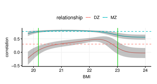
Figure 5: Estimated monozygotic (MZ) and dizygotic (DZ) twins correlation curves for the BMI data, with pointwise 95% confidence intervals (in grey). The dashed lines display the (overall) Pearson correlation within MZ and DZ twin pairs, respectively. The vertical green lines represent the $0.05$ and $0.95$ quantiles of the data.

Figure 5 displays the estimated correlation curve for both MZ and DZ twins, using the parameter values from Table 2. Also shown are 95% confidence intervals calculated using the delta method. Both correlation curves are fairly flat within the center 90% data range (represented by the two vertical green bars), while they both drop for low and high BMI. This yields (Figure 6) an estimated heritability curve $a^{2}(y)$ that does not differ significantly (except maybe around $y=22.3$) from the classical heritability coefficient (2.1.1).

The TMB (R and C++) code used to produce the parameter estimates in Table 2 plots in Figure 6 is available from https://github.com/skaug/Supplementary.

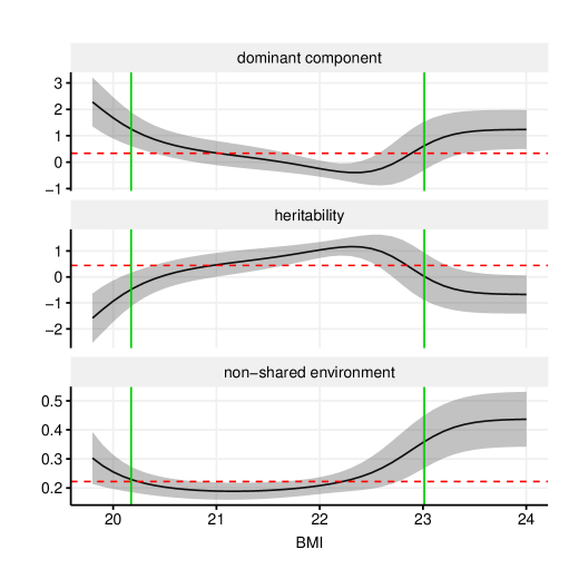
Figure 6: Estimated dominant genetic component $d^{2}(y)$, heritability curve $a^{2}(y)$, and environment curve $c^{2}(y)$ for the BMI data under the ADE model (Definition 1), with pointwise 95% confidence intervals (in grey). The red dashed lines display the classical estimates of dominant component, heritability, and environment, given by (2.1.1). The vertical green lines represent the $0.05$ and $0.95$ quantile in data.

4.2 Birth weight of family trios

To illustrate the family trio analyses, we used birth weights of $n=81,144$ complete mother–father–child trios. The data originally derived from the Medical Birth Registry of Norway, where the birth weight variables were added some random noise and rounded off to guarantee anonymity. The same data with some additional restrictions on parity, plurality, etc. were previously described and analyzed elsewhere (Magnus et al., , 2001). The data were restricted to all births (mother, father, and child) taking place within the years 1967–1998. Due to Norwegian ethical and legal restrictions, Norwegian data used in this study are available upon request to the Medical Birth Registry of Norway, the Norwegian Institute of Public Health. URL: https://www.fhi.no/hn/helseregistre-og-registre/mfr. Requests for data access can be directed to Datatilgang@fhi.no¡mailto:Datatilgang@fhi.no¿.

We did not have information about the gender of the child; hence, we performed a standardization of the data. We assumed a $50\%$ sex ratio in the offspring, and introduced the quantity $D\triangleq\frac{1}{2}\left(\bar{y}_{M}-\bar{y}_{F}\right)$, where $\bar{y}_{M}$ is the mean of the birth weights of mothers, and $\bar{y}_{F}$ is the mean of the birth weights of fathers. We hence added $D$ to the father’s weight and subtracted it to the mother’s weight; in this way, the average among mothers and fathers is the same, and close (25g deviation) to the average in the offspring. This standardization is of little consequence to the end result.

Figure 1 summarizes the marginal and bivariate properties of the data. The marginal distributions are close to a Gaussian shape, but the left tail of the child birth weights is slightly heavier than the right tail. As suggested in the Introduction, this may be indicative of strong but rare factors dominating in producing the lowest birth weigths, which is what we will confirm in our analyses of local heritability below.

The scatter plots are roughly symmetric around the identity line, which is consistent with the exchangeability assumption made in Section 2.2. It should be noted, however, that the left hand tail of the marginal distributions is somewhat heavier in the children than in the parents; this is likely because parents are selected by the fact that they have children; it is known that individuals born with low birth weight have somewhat reduced fertility later in life. We have, however, not taken this into consideration in our model.

From the non-parametric regression (blue curve), it is clear that there is no association between mother and father, which is reflected in the low Pearson correlation of $0.0209$. For the two relationships involving the child, the non-parametric regression curve indicates a non-linear relationship, particularly for mother-child. For birth weights less than 3000g there seems to be a low association, while for larger birth weights the association is increasing.

The Gaussian mixture (3.1) was fit by maximum likelihood for $m=1,\ldots,7$. We computed both AIC and BIC values for this model. According to the BIC criterion, the best fitting mixture has $m=4$ components (see Table 3). Parameters estimates for this model are given in Table 4. Figure 7 shows the underlying mother-child pairs, overlaid by the five mixture components.

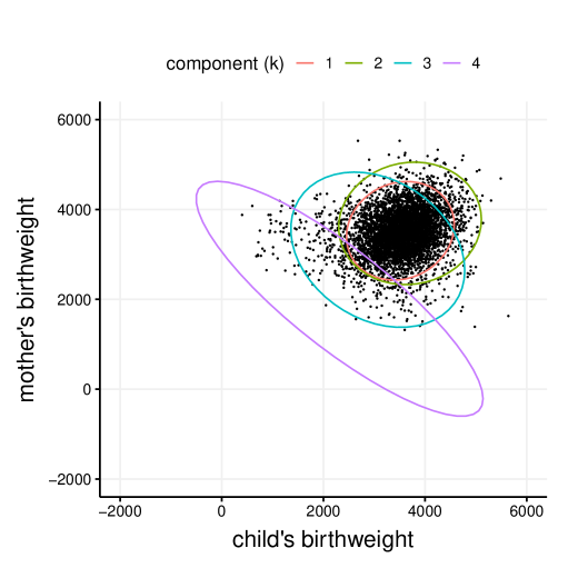
Figure 7: Birth weight (gram) of a random subset of $5000$ mother-child pairs taken from Figure 1. Also shown are 95% level curves (ellipses) for each of the $m=4$ mixture components in Table 4, i.e. each elipse include 95% of the probability mass for that bivariate normal component.

$m$	no. parameters	$\Delta$ AIC	$\Delta$ BIC
$1$	$5$	14848	14749
2	11	1148	904.4
3	17	480.4	292.5
4	23	132.1	0
5	29	109.7	33.5
6	35	36.3	16.0
7	41	0	35.5

Table 3: Model comparison for family trios, where $m$ is the number of mixture components. The total number of (free) parameters is $6m-1$, counting all $p_{k}$, $\mu_{k}$, $\sigma_{k}$, $\rho_{k}^{(MC)}$, $\rho_{k}^{(FC)}$ and $\rho_{k}^{(MF)}$. AIC and BIC values are relative to the lowest one, represented in red.

The mother-child distribution is pear-shaped relative to a bivariate normal distribution, with more spread around the identity line ($y_{1}=y_{2}$) for small birth weights. The mixture model adapts to this shape by assigning negative $\rho_{k}$’s to its two components ($k=3,4$) with the smallest $\mu_{k}$. The remaining two components ($k=1,2$), which together constitute 87% of the probability mass, form a bivariate distribution that is hard to distinguish visually from a Gaussian distribution. The estimates of global correlation for the mixture in Table 3, closely match the corresponding empirical Pearson correlations given in Figure 1 for MC, FC and MF pairs. It is seen to fit the empirical marginals fairly well, and to posses a heavier left hand tail.

Parameters	$k=1$	$k=2$	$k=3$	$k=4$	Global
$\mu_{k}$	3516	3687	3093	2243	3493
$\sigma_{k}$	440.5	572.9	690.5	1116	555.0
$\rho^{(MC)}_{k}$	0.240	0.143	$-$0.189	$-$0.826	0.123
$\rho^{(FC)}_{k}$	0.134	0.053	$-$0.254	$-$0.845	0.201
$\rho^{(MF)}_{k}$	$-$0.011	$-$0.084	$-$0.289	0.750	0.068
$p_{k}$	0.636	0.231	0.126	0.007

Table 4: Parameter estimates and standard deviations for the Gaussian mixture ($m=4$) fit to the mother–father–child trios. The mixture components are ordered according to the value of $\sigma_{k}$. The global quantities, $\mu$, $\sigma$, $\rho^{(MC)}$, $\rho^{(FC)}$ and $\rho^{(MF)}$ are calculated from (3.4).

Figure 8 shows the two estimated correlation curves $\rho^{(FC)}(y)$ and $\rho^{(MC)}(y)$, which are the components going into $a^{2}(y)$, $c^{2}(y)$, and $e^{2}(y)$, given respectively by (2.14)–(2.16). Overall, the Pearson correlation and the correlation curves for MF exceed those for FC. Both curves exceed their respective Pearson correlations in the center of the data, while they decrease for both low and high birth weights. The FC curve has its maximum somewhat to the left of the maximum of the MC curve. As a robustness check, we also computed the local Gaussian correlations  (Tjøstheim and Hufthammer, , 2013) between mother and child as displayed in Figure 9. These exhibit the same behaviour as the correlation curve; large values in the center of the data which are decreasing towards both tails. Figure 10 shows heritability and environment curves. The overall conclusion is that variation in birth weight is mostly attributable to environment, which was also seen in previous publications (Magnus et al., , 2001; Lunde et al., , 2007; Gjessing and Lie, , 2008), and is reflected in the classical measures of heritability $a^{2}=0.246$ and environment $c^{2}=0.754$, and the variation in the corresponding curves.

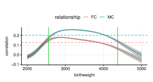
Figure 8: Estimated mother-child (MC) and father-child (FC) correlation curves for the Norwegian Birth Registry data, with pointwise 95% confidence intervals (in grey). The dashed lines display the (overall) Pearson correlation within MC and FC pairs, respectively. The vertical green lines represent the $0.05$ and $0.95$ quantiles of the data.

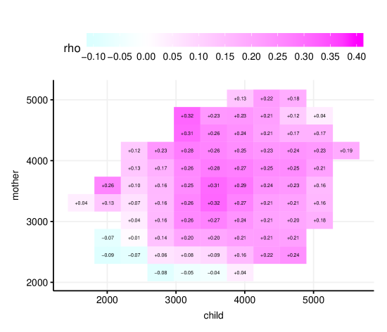
Figure 9: Estimated local Gaussian correlation between mother and child. Note that this correlation measure has two location arguments ($y_{1}$ and $y_{2}$).

Recall that, under the assumed model (2.7) the heritability curve $a^{2}(y)$ is completely determined by the FC correlation curve $\rho^{(FC)}(y)$. Since the FC correlation curve exceeds the Pearson FC correlation in the center of the data, the heritability curve also exceeds the classical heritability measure in the same region.

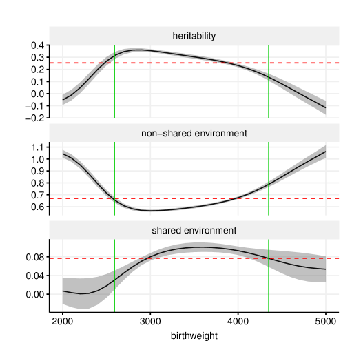
Figure 10: Estimated heritability curve $a^{2}(y)$, environment curve $c^{2}(y)$, and residual environment $e^{2}(y)$ for the Norwegian Birth Registry data under the ACE model (Definition 2), with pointwise 95% confidence intervals (in grey). The red dashed lines display the classical estimates of heritability and environment, i.e. empirical versions of (2.7). The vertical green lines represent the $0.05$ and $0.95$ quantiles of the data.

5 Discussion and conclusion

We have provided closed-form expressions for the correlation curve for exchangeable bivariate Gaussian mixtures. To our knowledge, this result is new and should be useful generally in situations where exchangeability can be assumed. Since differences in mean values may accounted for using a linear predictor like (2.5), it is only exchangeability of the residuals, or the weaker condition (2.2.2), that is required. In the context of our family data, the exchangeability assumption is rather reasonable for twin data. In nuclear families, it is less obvious that parents and children have the exact same marginal distribution even when using covariates to adjust for systematic generational differences. With our generational birth weight data, we observe that the left hand tail in the parental distribution is smaller than among the children. As discussed in Subsection 4.2, this may well be a selection phenomenon; somebody born with a very low birth weight is less likely to become a parent, and are thus possibly under-represented in our data file. For instance, increased mortality among the smallest newborns is thought to lead to a selection pressure on the birth weight distribution over generations (Cavalli-Sforza and Bodmer, , 1999).

A restriction of our model is that we have applied it only in situations with simple family structures where moment estimators of the heritability are explicit. In larger family structures, several pairwise relationships may provide information about the same heritability parameters. For instance, family trios with sibling data add the sibling correlation as a source of information (Lunde et al., , 2007). We will not discuss that issue further, but note that if pairwise correlation curves are estimated from larger data structures, weighted least squares estimation may provide a way of combining them into a common estimate of heritability curves (Gjessing and Lie, , 2008).

In our twin BMI example, we chose the ADE model for the estimation since for the estimated overall correlations, $\rho^{(MZ)}>2\rho^{(DZ)}$. However, as seen in Figure 6, there are values for $y$ (the BMI) where the estimated $d^{2}(y)$ drops below zero. This indicates that in this region, the ACE model might be more appropriate. Note that there is no difficulty in letting the local heritability curves switch from an ADE model to an ACE model locally. In particular, we see that when $\rho^{(MZ)}=2\rho^{(DZ)}$, both (2.1.1) and (2.1.1) provide the same estimates for $a^{2}$ and $e^{2}$, and both $c^{2}$ and $d^{2}$ are estimated as zero. The estimated heritability curves would thus still be continuous if switching from one model to another.

The choice of Gaussian mixtures was made due to their flexibility, in the spirit of non-parametric estimation. Our approach is pragmatic in the sense that we have not attempted to interpret individual mixture components as sub-populations. One reason for this is the negative estimates for some of the $\rho_{k}$ seen in both Table 2 and 4, which would be hard to interpret biologically.

On the other hand, Gaussian mixtures are fully parametric models, which allows us to use the standard parametric toolbox. For instance, covariates can easily enter the mean, as in (2.5), and it would also be straight forward to formulate model in which the $\sigma_{k}$ were affect by family level covariates. A further benefit of having a parametric model is that we can select model complexity ($m$) based on standard AIC or BIC criteria.

The parametric structure is also the basis for the results about the tail behaviour of the correlation curve in Theorem 3.1.1. While the center of the distribution may have sufficient data to allow stable non-parametric estimation of the heritability, the estimates in the tails are more dependent on the model structure. This is both a strength and a weakness of the mixture model. The heritability curves converge to constant values in the tails, which makes the estimates more stable; on the other hand, those estimates depend on the dominant mixture components in the tails, and the number and placement of mixture components may not always be clear cut.

There are also well known problems with Gaussian mixtures. Among these are local maxima on the likelihood surface  (Baudry and Celeux, , 2015), which can be explored by using different initial values for the numerical optimization. We avoided the classical “label switching” problem by constraining the parameters of the mixture ($\sigma$’s and $\mu$’s), but have nevertheless observed some sensitivity of the parameter estimates in Table 4. Although we cannot guarantee that we have found the global optimum of the likelihood surface, the choice of model complexity ($m$) seems to be robust to the choice of initial values. Similarly, the shape of the correlation curves (and consequently heritability and environment curves) are quite stable. A related problem is that of singlularity of the Fisher information matrix which can occur for mixture models (Drton and Plummer, , 2017). This could potentially affect the validity of AIC and BIC criteria, as well as the standard deviations based on the observed Fisher information that have been used throughout this paper. Such standard deviations are produced automatically by TMB, and are very convenient in an exploratory phase, but we recommend that they are validated by simulation (parametric bootstrap).

6 Acknowledgements

This research was supported by Research Council of Norway grant 225912/F50 “Health Registries for Research” and the Centres of Excellence funding scheme (Grant 262700).

Appendix A Proofs

Proof of Proposition 1.

Let $g(y)$, $g_{k}(y)$, $p_{k}^{*}(y)$ etc. be defined as in Section 3. First, note that

$$\frac{g_{k}^{\prime}(y)}{g_{k}(y)}=d_{k}(y).$$

Furthermore, define

$$d(y):=\sum_{i=1}^{m}p_{i}^{*}(y)d_{i}(y),$$

i.e. the weighted average of the $d_{i}(y)$’s. Then

$$\frac{g^{\prime}(y)}{g(y)}=\frac{\sum_{i=1}^{m}d_{i}(y)g_{i}(y)}{g(y)}=d(y).$$

For any fraction $s(y)=a(y)/b(y)$ of differentiable functions, note that the chain rule can be written as $\frac{s^{\prime}(y)}{s(y)}=\frac{a^{\prime}(y)}{a(y)}-\frac{b^{\prime}(y)}{b(y)}$. Thus,

$$\frac{p_{k}^{*^{\prime}}(y)}{p_{k}^{*}(y)}=\frac{g_{k}^{\prime}(y)}{g_{k}(y)}-\frac{g^{\prime}(y)}{g(y)}=d_{k}(y)-d(y).$$

Recall from (3.6) that $\mu(y)=\operatorname{E}\left[Y_{1}\mid Y_{2}=y\right]=\sum_{i=1}^{m}p_{i}^{*}(y)\mu_{i}(y)$ is the conditional expectation,

$$\beta(y)=\mu^{\prime}(y) =\sum_{i=1}^{m}\left(p_{i}^{*}(y)\mu{}_{i}^{\prime}(y)+p_{i}^{*^{\prime}}(y)\mu_{i}(y)\right)$$

$$=\sum_{i=1}^{m}p_{i}^{*}(y)\left(\rho_{i}+\mu_{i}(y)\left(d_{i}(y)-d(y)\right)\right)$$

$$=\sum_{i=1}^{m}p_{i}^{*}(y)\left(\rho_{i}+\left(\mu_{i}(y)-\mu(y)\right)\left(d_{i}(y)-d(y)\right)\right)$$

$$=\sum_{i=1}^{m}p_{i}^{*}(y)\left(\rho_{i}+\left(\mu_{i}(y)-\mu(y)\right)d_{i}(y)\right),$$

where we make use of $\sum_{i=1}^{m}p_{i}^{*}(y)\left(d_{i}(y)-d(y)\right)=0$ and $\sum_{i=1}^{m}p_{i}^{*}(y)\left(\mu_{i}(y)-\mu(y)\right)=0$.

∎

A.0.1 Proof of Theorem 3.1.1 - asymptotic behavior of $\beta(y)$, $\sigma^{2}(y)$, and $\rho(y)$

For two functions $a(y)$ and $b(y)$, as $y\to\infty$ (or $-\infty$), we use the standard notation that $a(y)\sim b(y)$ means $\lim_{y\to\infty}a(y)/b(y)=1$, and $a(y)\ll b(y)$ means $\lim_{y\to\infty}a(y)/b(y)=0$. Our proofs below follow mostly from standard theory on asymptotic behavior of real functionsBender and Orszag, (2013).

Asymptotic behavior of mixture components

For one mixture component $g_{k}(y)$, the asymptotic behavior when $y\to\pm\infty$ is

$$g_{k}(y)\sim C_{k}\exp\left(\frac{\mu_{k}}{\sigma_{k}}y-\frac{1}{2\sigma_{k}^{2}}y^{2}\right),$$

for a constant $C_{k}$. Comparing two components $g_{k}(y)$ and $g_{l}(y)$ with $\sigma_{k}^{2}<\sigma_{l}^{2}$, we clearly have

$$g_{k}(y)\ll g_{l}(y)\quad\text{as}\quad y\to\pm\infty$$ (A.1)

since the $y^{2}$-term dominates the asymptotics. If $\sigma_{k}^{2}=\sigma_{l}^{2}$, assume that $\mu_{k}<\mu_{l}$. Then

$$g_{k}(y)\ll g_{l}(y)\quad\text{as}\quad y\to+\infty,$$ (A.2)

and

$$g_{l}(y)\ll g_{k}(y)\quad\text{as}\quad y\to-\infty.$$ (A.3)

Let $a_{k}(y)$ be non-zero polynomial functions in $y$ for $k=1,\ldots,m$. Since polynomials are asymptotically dominated by exponentials of polynomials, the products $g_{k}(y)a_{k}(y)$ are asymptotically ordered in the same way as in (A.1), (A.2), and (A.3) above.

Asymptotic behavior of mixtures

Recall the definition of $K$ in Theorem 3.1.1. The results above apply directly to the sum $\sum_{k=1}^{m}g_{k}(y)a_{k}(y)$, which will asymptotically follow the dominant term with $k=K$. I.e.,

$$\sum_{k=1}^{m}g_{k}(y)a_{k}(y)\sim g_{K}(y)a_{K}(y).$$

In particular, for the full density we get

$$g(y)=\sum_{i=1}^{m}g_{i}(y)\sim g_{K}(y).$$

Similarly, if $k\neq K$,

$$p_{k}^{*}(y)a_{k}(y)=\frac{g_{k}(y)a_{k}(y)}{g(y)}\to 0,$$ (A.4)

and

$$p_{K}^{*}(y)a_{K}(y)\sim a_{K}(y).$$

Conditional mean $\mu(y)$

Applying the above results to $\mu$, we obtain

$$\mu(y)=\sum_{k=1}^{m}p_{k}^{*}(y)\mu_{k}(y)\sim\mu_{K}(y)\sim\rho_{K}\cdot y.$$

Furthermore, letting $a_{k}(y)=\rho_{k}+\left(\mu_{k}(y)-\mu(y)\right)d_{k}(y)$, we get

$$\beta(y)=\sum_{k=1}^{m}p_{k}^{*}(y)a_{k}(y)\sim a_{K}(y).$$

However, by A.4,

$$\left(\mu_{K}(y)-\mu(y)\right)d_{K}(y)=\sum_{k=1}^{m}p_{k}^{*}(y)(\mu_{K}(y)-\mu_{k}(y))d_{K}(y)\to 0$$

since the $K$’th term vanishes. It follows that

$$\beta(y)\sim a_{K}(y)\to\rho_{K}.$$

Conditional variance $\sigma^{2}(y)$

For the conditional variance,

$$\sigma^{2}(y) =\sum_{k=1}^{m}p_{k}^{*}(y)\left[\sigma_{k}^{2}(1-\rho_{k}^{2})+\left[\mu_{k}(y)-\mu(y)\right]^{2}\right]$$

$$\sim\sigma_{K}^{2}(1-\rho_{K}^{2}).$$

Correlation curve $\rho(y)$

Finally, the result for the correlation curve $\rho(y)$ follows directly from the results for $\sigma^{2}(y)$ and $\beta(y)$.

References

- Baudry and Celeux, (2015) Baudry, J.-P. and Celeux, G. (2015). Em for mixtures. Statistics and computing, 25(4):713–726.
- Bender and Orszag, (2013) Bender, C. M. and Orszag, S. A. (2013). Advanced Mathematical Methods for Scientists and Engineers I: Asymptotic Methods and Perturbation Theory. Springer Science & Business Media. Google-Books-ID: xz0mBQAAQBAJ.
- Bjerve and Doksum, (1993) Bjerve, S. and Doksum, K. (1993). Correlation curves: Measures of association as functions of covariate values. Ann. Statist., 21(2):890–902.
- Bulmer, (1985) Bulmer, M. G. (1985). The Mathematical Theory of Quantitative Genetics. Clarendon Press.
- Cavalli-Sforza and Bodmer, (1999) Cavalli-Sforza, L. L. and Bodmer, W. F. (1999). The Genetics of Human Populations, pages 612–614. Courier Corporation.
- (6) Cherny, S., Cardon, L., Fulker, D. W., and DeFries, J. (1992a). Differential heritability across levels of cognitive ability. Behavior genetics, 22(2):153–162.
- (7) Cherny, S. S., Cardon, L. R., Fulker, D. W., and DeFries, J. C. (1992b). Differential heritability across levels of cognitive ability. Behavior Genetics, 22(2):153–162.
- DeFries and Fulker, (1985) DeFries, J. C. and Fulker, D. W. (1985). Multiple regression analysis of twin data. Behavior genetics, 15(5):467–473.
- DeFries and Fulker, (1988) DeFries, J. C. and Fulker, D. W. (1988). Multiple regression analysis of twin data: Etiology of deviant scores versus individual differences. Acta Geneticae Medicae et Gemellologiae: Twin Research, 37(3-4):205–216.
- Doksum et al., (1994) Doksum, K., Blyth, S., Bradlow, E., Meng, X.-L., and Zhao, H. (1994). Correlation Curves as Local Measures of Variance Explained by Regression. Journal of the American Statistical Association, 89(426):571–582.
- Drton and Plummer, (2017) Drton, M. and Plummer, M. (2017). A bayesian information criterion for singular models. Journal of the Royal Statistical Society: Series B (Statistical Methodology), 79(2):323–380.
- Falconer, (1960) Falconer, D. S. (1960). Introduction to quantitative genetics. Oliver And Boyd; Edinburgh; London.
- Fisher, (1919) Fisher, R. A. (1919). XV.—The Correlation between Relatives on the Supposition of Mendelian Inheritance. Earth and Environmental Science Transactions of The Royal Society of Edinburgh, 52(2):399–433. Publisher: Royal Society of Edinburgh Scotland Foundation.
- Gjessing and Lie, (2008) Gjessing, H. K. and Lie, R. T. (2008). Biometrical modelling in genetics: are complex traits too complex? Statistical Methods in Medical Research, 17(1):75–96. PMID: 17855744.
- Holland and Wang, (1987) Holland, P. W. and Wang, Y. J. (1987). Dependence function for continuous bivariate densities. Communications in Statistics - Theory and Methods, 16(3):863–876.
- Hopper, (2002) Hopper, J. L. (2002). Heritability. In Elston, R., Olson, J., and Palmer, L., editors, Biostatistical Genetics and Genetic Epidemiology, Wiley reference series in biostatistics, pages 371–372. Wiley, West Sussex, UK.
- Hopper and Visscher, (2002) Hopper, J. L. and Visscher, P. M. (2002). Genetic Correlations and Covariances. In Elston, R., Olson, J., and Palmer, L., editors, Biostatistical Genetics and Genetic Epidemiology, Wiley reference series in biostatistics, pages 327–331. Wiley, West Sussex, UK.
- Khoury et al., (1993) Khoury, M. J., Beaty, T. H., and Cohen, B. H. (1993). Fundamentals of Genetic Epidemiology. Oxford University Press.
- Kristensen et al., (2016) Kristensen, K., Nielsen, A., Berg, C. W., Skaug, H., and Bell, B. M. (2016). Tmb: Automatic differentiation and laplace approximation. Journal of Statistical Software, 70(1):1–21.
- LaBuda et al., (1986) LaBuda, M. C., DeFries, J., Fulker, D. W., and Rao, D. (1986). Multiple regression analysis of twin data obtained from selected samples. Genetic epidemiology, 3(6):425–433.
- (21) Logan, J. A., Petrill, S. A., Hart, S. A., Schatschneider, C., Thompson, L. A., Deater-Deckard, K., DeThorne, L. S., and Bartlett, C. (2012a). Heritability across the distribution: An application of quantile regression. Behavior genetics, 42(2):256–267.
- (22) Logan, J. A., Petrill, S. A., Hart, S. A., Schatschneider, C., Thompson, L. A., Deater-Deckard, K., DeThorne, L. S., and Bartlett, C. (2012b). Heritability Across the Distribution: An Application of Quantile Regression. Behavior genetics, 42(2):256–267.
- Lunde et al., (2007) Lunde, A., Melve, K. K., Gjessing, H. K., Skjærven, R., and Irgens, L. M. (2007). Genetic and Environmental Influences on Birth Weight, Birth Length, Head Circumference, and Gestational Age by Use of Population-based Parent-Offspring Data. American Journal of Epidemiology, 165(7):734–741.
- Magnus et al., (2001) Magnus, P., Gjessing, H. K., Skrondal, A., and Skjærven, R. (2001). Paternal contribution to birth weight. Journal of Epidemiology & Community Health, 55(12):873–877.
- McCulloch and Neuhaus, (2001) McCulloch, C. E. and Neuhaus, J. M. (2001). Generalized linear mixed models. Wiley Online Library.
- McLachlan and Peel, (2000) McLachlan, G. and Peel, D. (2000). Finite mixture models. Wiley New York.
- Neale, (2002) Neale, M. C. (2002). Twin Analysis. In Elston, R., Olson, J., and Palmer, L., editors, Biostatistical Genetics and Genetic Epidemiology, Wiley reference series in biostatistics, pages 206–217. Wiley, West Sussex, UK.
- Neale et al., (2016) Neale, M. C., Hunter, M. D., Pritikin, J. N., Zahery, M., Brick, T. R., Kirkpatrick, R. M., Estabrook, R., Bates, T. C., Maes, H. H., and Boker, S. M. (2016). Openmx 2.0: Extended structural equation and statistical modeling. Psychometrika, 81(2):535–549.
- Pawitan et al., (2004) Pawitan, Y., Reilly, M., Nilsson, E., Cnattingius, S., and Lichtenstein, P. (2004). Estimation of genetic and environmental factors for binary traits using family data. Statistics in Medicine, 23:449–465.
- Rabe-Hesketh et al., (2008) Rabe-Hesketh, S., Skrondal, A., and Gjessing, H. (2008). Biometrical modeling of twin and family data using standard mixed model software. Biometrics, 64(1):280–288.
- Tjøstheim and Hufthammer, (2013) Tjøstheim, D. and Hufthammer, K. O. (2013). Local gaussian correlation: A new measure of dependence. Journal of Econometrics, 172(1):33 – 48.
- Wright, (1920) Wright, S. (1920). The relative importance of heredity and environment in determining the piebald pattern of guinea-pigs. Proceedings of the National Academy of Sciences of the United States of America, 6(6):320–332. Publisher: National Academy of Sciences.
- Wright, (1921) Wright, S. (1921). Correlation and causation. Journal of agricultural research, 20(7):557–585.