a)
![[Uncaptioned image]](/html/2004.08475/assets/x1.png) b)
b)
![[Uncaptioned image]](/html/2004.08475/assets/x2.png) c)
c)
![[Uncaptioned image]](/html/2004.08475/assets/teaser2.png)
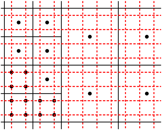
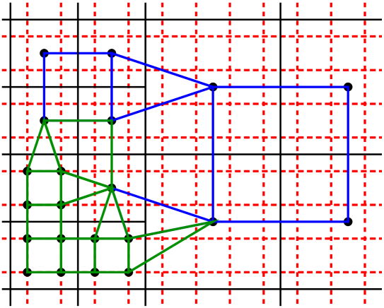
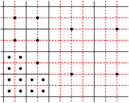
a) Given an arbitrary set of invidiual AMR cells (that could come from either block-structured or octree AMR data) out method provides an easy, programmatically simple, and trivially parallel way of computing all cells of the dual mesh (b), which can then, for example be fed into the Marching Cubes case tables to produce a crack-free polygonal iso-surface. c) A 130 million triangle iso-surface ( field, ) of the NASA Exajet model, which consists of individual AMR cells (with holes, and without any apparent hierarchy). Computing this surface with a CUDA implementation of our method took 8.4 seconds on a NVIDIA RTX 8000 GPU.
A Simple, General, and Parallel Method for
Extracting Crack-free
Iso-Surfaces from
Adaptive Mesh Refinement (AMR) Data
A Simple, General, and GPU Friendly Method for
Computing Dual Mesh and Iso-Surfaces of
Adaptive Mesh Refinement (AMR) Data
Abstract
We propose a novel approach to extracting crack-free iso-surfaces from Structured AMR data that is more general than previous techniques, is trivially simple to implement, requires no information other than the list of AMR cells, and works, in particular, for different AMR formats including octree AMR, block-structured AMR with arbitrary level differences at level boundaries, and AMR data that consist of individual cells without any existing grid structure. We describe both the technique itself and a CUDA-based GPU implementation of this technique, and evaluate it on several non-trivial AMR data sets.
1 Introduction
Adaptive Mesh Refinement (AMR) was first introduced by Berger et al. [BO84, BC89], and has since become one of the most widely used methods for scientific simulation codes. Its base idea is that a initially coarse domain subdivision gets adaptively refined based where the simulation has the most need for finer discretization—which significantly reduces the number of discretization elements (and thus, memory storage) required to reach a certain accuracy.
Visualizing such data often requires the computation of a polygonal iso-surface over this data; this can then be rendered, typically color-mapped with one or more additional attributes. Unfortunately, computing crack-free iso-surfaces can be challenging due to the irregular nature of the AMR cells; in particular, the dual mesh of a structured AMR data set is a unstructured mesh that in the general case can contain unstructured elements ranging from tetrahedra to non-rectangular hexahedra with curved sides.
Today, the best known method for computing crack-free iso-surfaces of AMR data is what we call the “stitching” method by Weber et al. [WKL∗03, WCM12]: this method walks the brick boundaries, and stitches these with unstructured elements that are picked by using pre-computed case tables. This method is widely used, but relies on certain assumptions—in particular, that the input is block-structured AMR with no more than one level differences at block boundaries—that are not always met even for block-structured AMR, and not at all for octree-AMR. Furthermore, the non-trivial case tables make this method challenging to implement.
An alternative—but apparently less well known—solution to this problem was introduced by Moran at al. [ME11], who observe that placing epsilon-sized boxes around all vertices of the input mesh, and “snapping” the corners of those epsilon boxes to the centers of the cells they lie in (for which they use a cell location kernel that walks the brick hierarchy), will produce exactly the unstructured cells of the dual mesh. This method is more general, but apparently little known, arguably because it is mentioned only as an aside in a paper with an otherwise different focus.
Contributions. In this paper, we propose a method that—though originally developed independently—can be viewed as a simpler re-formulation of the Moran method. In particular, using a well-defined integer labeling scheme for both cells and dual cells our method avoid Moran’s epsilon-offsetting, and reduces their cell location kernel to simple binary search of integer indices; it is easy to implement, trivially parallelizable on a per-cell basis, and lends itself naturally to a GPU implementation. Like Moran’s method, our method works on both octree AMR and structured AMR data (including arbitrary level differences and “holes” in the model), and can be used for either dual-mesh and/or iso-surface generation. We also detail a CUDA reference implementation of this method (which will be shared with this paper), and demonstrate that this can extract crack-free iso-surfaces of even complex AMR data sets in a matter of seconds (see Figure A Simple, General, and Parallel Method for Extracting Crack-free Iso-Surfaces from Adaptive Mesh Refinement (AMR) Data ).
2 Related Work
Cell-centered AMR was first introduced by Berger and Oliger [BO84] and Berger and Colella [BC89], and in one or another form today is used in a wide range of scientific simulation codes such as, for example, Chombo [CGL∗00], Flash [FOR∗00], LAVA [KBH∗14], Rage [GWC∗08], and many others. In particular, though originally introduced in the form of block-structured AMR where different-resolution grids are layered on top of each other, today there are different variants ranging from block-structured to octree-style AMR. Though the actual structure of the resulting AMR mesh can vary wildly between those codes, they all follow certain rules in that refinement happens in power-of-two factors, with data values defined only for the center of each cell, and with certain rules regarding how refined cells have to align to coarser ones [BO84, BC89].
One of the first approaches to visualize AMR data was proposed by Weber et al [WKL∗03], who proposed to first construct the dual mesh, and extract an iso-surface from that the Marching Cubes [LC87] case tables. To construct the dual messh Weber proposed to walk along the boundaries of the input bricks, and “stitching” across level boundaries with elements such as tetrahedra, pyramids, using a case table of some 36 different cases to determine which element shape(s) to pick at any given point. Notwithstanding some refinements (e.g., [WCM12]) this method has remained the de facto standard method for nearly two decades; its main downside is that it requires some existing grid hierarchy, and in particular, that models not contain any cases where more than two different levels abut, as this would require significantly more complex case tables.
A significantly less known technique for computing this dual mesh was proposed by Moran et al. [ME11], in the context of computing an interpolant for high-quality AMR volume rendering. In their paper, Moran et al. observe that there is a one-to-one correspondence between vertices in the AMR mesh and unstructured cells in the dual mesh on one hand, and input cell centers and dual mesh vertices on the other—and that the dual mesh can thus be constructed by surrounding each input mesh vertex with a tiny box whose vertices then get snapped to the centers of the cells they lie in. To do this snapping they proposed cell location kernel that walks a hierarchy of AMR bricks. Though more general than Weber’s, this technique seems significantly less known, arguably because it was not primarily proposed for iso-surface extraction. Though developed independently—and with slightly different rationale—our method is similar in spirit, and may actually best be viewed as a simpler re-formulation of this technique.
A way of computing a indexed triangle mesh from a set of “fat” triangles has been previously proposed by Bell [Bel10], with a follow-up improvement by Miller et al. [MMM14]. The concept of dual contouring has also been used, for example, by Nielsen [Nie04], Schaefer et al. [SW04], Kitware [SGLZ11], and Carrard et al [CLP12].
(a)
 (b)
(b)
 (c)
(c)
 (d)
(d)
 (e)
(e)
 (f)
(f)
 (g)
(g)
(a)
 (b)
(b)
(c)
 (d)
(d)
3 Terminology and Prerequisites
Though we use a different way of creating the dual mesh, at the root out method works the same way as proposed by Weber: First construct the dual mesh, then use that to extract the iso-surface. The key contribution of this paper is the formulation of how the dual mesh is constructed. To do this we first introduce a simple terminology for logical AMR cells, dual cells, and levels, with which the final method can be expressed in but a few lines of code.
3.1 Cells, Dual Cells, and Terminology used in this Paper
Throughout this paper we adopt a terminology where differentiate between logical and actual AMR cells, where logical cells refer to any cell that an AMR refinement count potentially produce, and actual cells as those logical cells used by an actual AMR data set. Due to the nature of AMR, all logical cells of any given refinement level form an infinite structured grid, which we call a “level”. In particular, throughout this paper we assume that level 0 is the finest level, with a cell size of 1; level 1 is the next coarser level with cell size of 2, etc. I.e., cells on level have a cell size of , and have coordinates that are multiples of . To identify cells we refer to them through four coordinates , with () being that cell’s lower-left corner, and the level on which it lives. Ie, each logical cell spans the space and is centered at .
All logical level--cells form an infinite grid of -sized cells, which implied a similar logical dual grid of dual cells , which we define as spanning from to .
Using this terminology any given AMR data set can then be descibed by which actual cells it contains, and what data value(s) these cells carry. Note in particular that we do not assume any existing block structure or hierarchy; just that we know which cells a given data set contains.
3.2 Efficient Cell Location
Given such a data set, in the later stages of our algorithm we assume that there will be a fast cell location operator snap(C) that finds, for any given set of cell coordinates , the actual input cell that contains the coordinates , or, if no such actual data set cell exists, a special “does not exist” indicator . Note in particular that the actual cell for the queried coordinates does not have to have these logical cell coordinates, but can absolutely be on either a finer or coarser level.
In our implementation we implement this operator by first sorting the set of input cells by their integer coordinates , and by determining the maximum number of levels . With this sorted array we can then quickly check if the data set contains a given cell with coordinates by simply running a binary search, for which in our implementation we use thrust’s thrust::lower_bounds [BH12].
For any given integer position we can then find the actual cell containing these coordinates—if it exists—by simply iterating over all levels; for each level we first project to valid level- cell coordinates by zeroing the lower bits of , , and , then perform the binary search. If any tested level finds an actual cell with these coordinates this is the cell we have been looking for; otherwise we return a . Of course, if we have a good guess on what level the queried cell might be on we can test this level first, saving some additional searches. Note in particular that we never need any floating-point coordinates, epsilons, or hierarchies, only pre-sorted integer cell coordinates. Furthermore, we make no distinctions between “inner” and “boundary” cells whatsoever; all cells are treated exactly the same, simplifying the algorithms and aiding parallelism.
4 Computing the Dual Mesh using Degenerate Dual Cells
Using this terminology and “cell location” kernel we now make the same argument as already made by Moran et al, namely, that snapping the vertices of logical dual cells to the centers of the actual cells they lie in will produce exactly the unstructured dual cells.
4.1 Conceptual Construction on the Finest Level
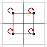
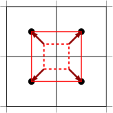
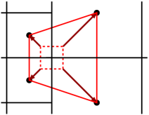
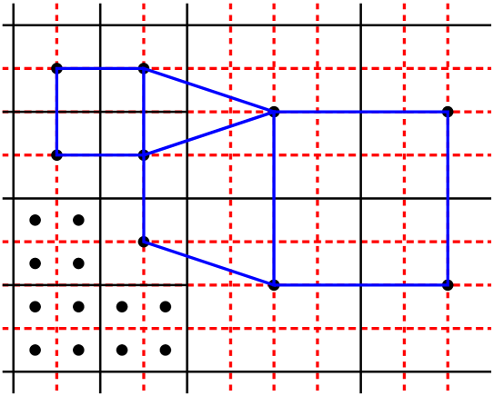
To illustrate the latter, let us first consider the 2D case, and at least for now, let us consider all(!) finest-level dual cells. In Figure 1 we have illustrated several cases on how an originally square-shaped finest-level dual snaps in different regions of a data set: In a finest-level region that square just snaps to itself (a); in coarser regions it either snaps to a larger square (b), to a line (c), or a point (d), depending on whether the dual square covers a coarser cell vertex (b), straddles and edge (c), or lies within a coarser cell (d).
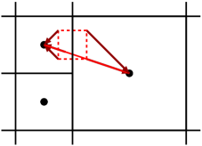
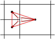
Along level boundaries, the shapes produced by snapping get more diverse, but still follow the same concept: in 2D, snapping a finest-level dual that straddles a level boundary can also produce a triangle (e) or trapezoid (f) along a simple boundary between only two levels; and a general quadrilateral if more than two different levels are involved (g). In 3D exactly the same construction applies, except that the shapes produced get even more diverse by adding another dimension: generally speaking, in the simple case inside a homogeneous regions 2D squares becomes 3D cubes, but along boundaries triangles and trapezoids can become tetrahedra, pyramids, wedges, or general hexahedra. Some of these shapes are non-trivial, as some of the hexahedra, wedges and pyramids can have faces that are non-flat bilinear patches.
In particular, we point out that this snapping does not make any assumptions as to how many different levels are involved, how big the level differences are, etc. Obviously, if any of the vertices does not snap to any actual cell the shape is not part of the dual mesh, and can be ignored.
4.2 Efficient Construction
Though constructing the dual mesh by snapping all finest-level cells does indeed work, for complex models it would be very inefficient to do so: for example, for the NASA Landing Gear Model outlined in Figure 3, the logical finest-level grid contains cells, translating to roughly quadrillion finest-level duals that we would need to snap.
However, as already pointed out by Moran et al. all that is required to find all shapes is that the snapped shapes cover all vertices of the input mesh. We further observe that every vertex of the input mesh is by definition one of the eight vertices of an actual cell , and as such, at the center of one of the eight logical dual cells () that cover this cells. This suggests that all we have to do is to generate, for each actual input cell , the coordinates of its 8 dual cells, and snap those.
4.3 Avoiding Duplicates
This method of snapping every actual cell’s eight duals is simple and correct, but since dual cells are generally shared among many different actual cells would naively generate each output cell several times. One way to avoid this would be to explicitly tag vertices that have already been processed, but this would require additional bookkeeping that would complicate the algorithm and in particular hamper parallelism.
Fortunately, we can easily avoid duplicates using a set of three simple rules that disambiguate which logical dual cell is allowed to produce the shape:
- rule #1
-
if any of the corners of the dual does not snap to any actual cells, then this dual does not produce a valid shape at all
- rule #2
-
if any of the corners of dual cell snaps to a finer level, then that same shape will already be produced on that finer level, and will not be emitted.
- rule #3
-
if any of the eight vertices of snaps to a cell that is on the same level , but has with coordinates lower than , then that same shape will already be produced by dual , and will not be emitted.
These conditions are trivial to test with just a few integer compares, and guarantee that every dual shape will get emitted exactly once.
4.4 Pseudo-Code
Though the previous sections was intentionally verbose, the resulting algorithm is intriguingly simple. For each of a cell’s 8 dual cells we construct the eight vertices, snap them, and reject the generated shape if it violates any of the previous three simple rules:
We observe that the entire construction is completely parallel, without any locks or synchronization whatsoever. In our actual CUDA implementation (see below) we launch one thread per each of the 8 dual cells for any of the inputs, and simply run the above code, using the fast cell location kernel outlined above.
5 Application to Iso-Surface Extraction
The construction discussed so far is general, and generates the dual mesh irrespective of its application to iso-surface extraction. As done by Moran et al, the resulting dual mesh, could, for example, be stored, and used to create an interpolant for direct volume rendering. However, an even easier application is iso-surface extraction. For this, the key observation is that though some of the snapped dual cells may degenerate to wedges, tetrahedra, pyramids, or even just lines or points we can still treat all of those shapes (even the degenerate ones) as if they were hexahedra, and simply feed those into the marching cubes (MC) algorithm.
That some of those hexahedras’ vertices have snapped to the same cell does not matter for the MC case tables at all: MC generates all of its surface vertices along edges of the hexahedra that have one vertex above and one below the desired iso-surface; in the case where edges snap to a single vertex both endpoints of that “edge” will by definition be the same, so triangles will never be generated along collapsed edges. Similarly, even if a face snaps to a non-trivial shape such as a triangle or even a bi-linear patch we know that both duals that share this face will have generated it in exactly the same way, thus the MC tables will place the respective shape’s vertices along that face at exactly the same locations, thus guaranteeing that no cracks can occur.
We observe that once again the entire process in our formulation is intriguingly simple: start one thread per each of the duals of the actual input cells, have that thread compute “its” dual cell, and if found, feed the resulting eight vertices—denegerate or not—into the standard MC case tables, then simply check which of the up to three generated triangles have three different vertices. As evidenced by the accompanying CUDA code the entire algorithm can be formulated in about as many lines of code as taken up by the MC case tables.
5.1 CUDA Implementation
 |
 |
 |
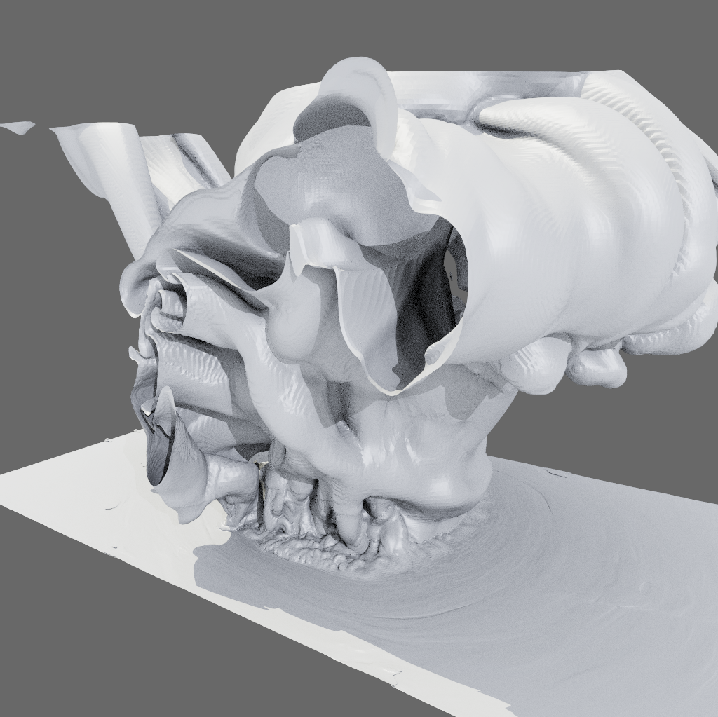 |
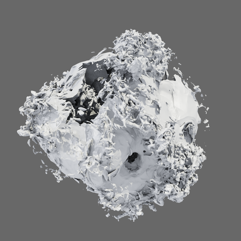
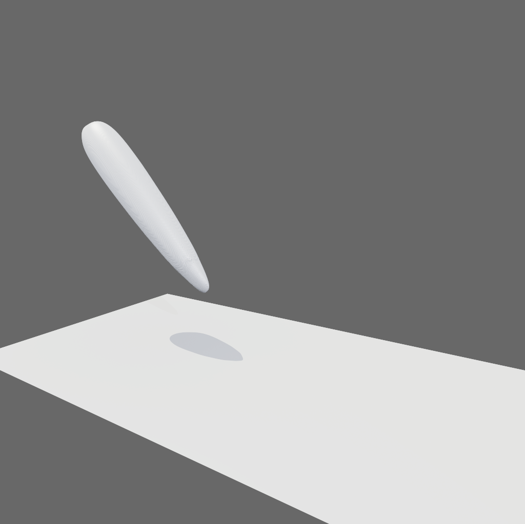
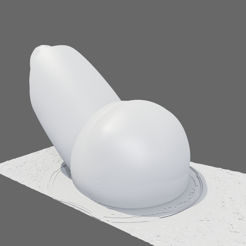
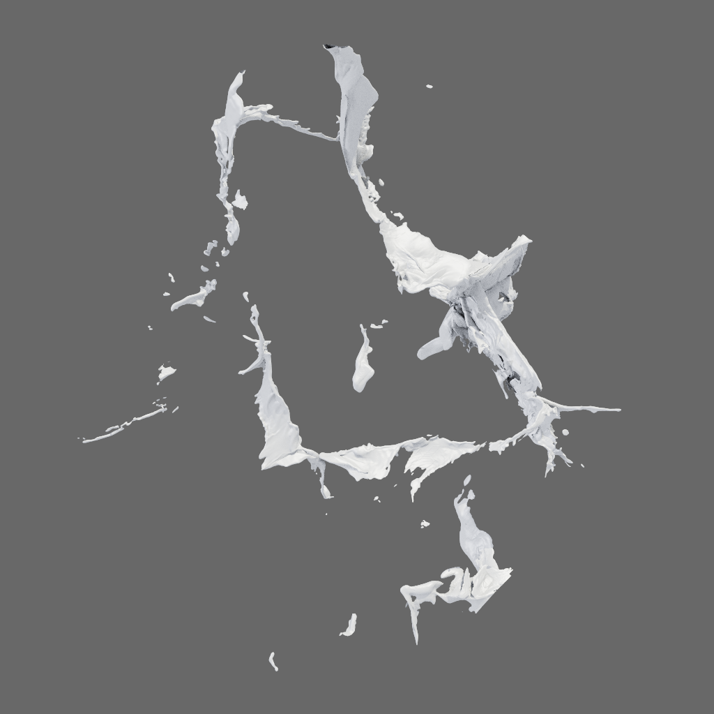
| stellar cluster wind | impact-5700 | impact-20060 | impact-46112 |
| (flash, block-structured) | (xRage, octree-AMR) | (xRage, octree-AMR) | (xRage, octree-AMR) |
| 4 levels, 77M cells | 4 levels, 26M cells | 4 levels, 151M cells | 4 levels, 270M cells |
| field, | field, | field, | field, |
| 24.3M triangles, 5.7/14.1 sec | 308K triangles, 0.38/0.91 sec | 2.3M triangles, 2.3/5.5 sec | 5.1M triangles, 3.8/9.4 sec |
 |
 |
 |
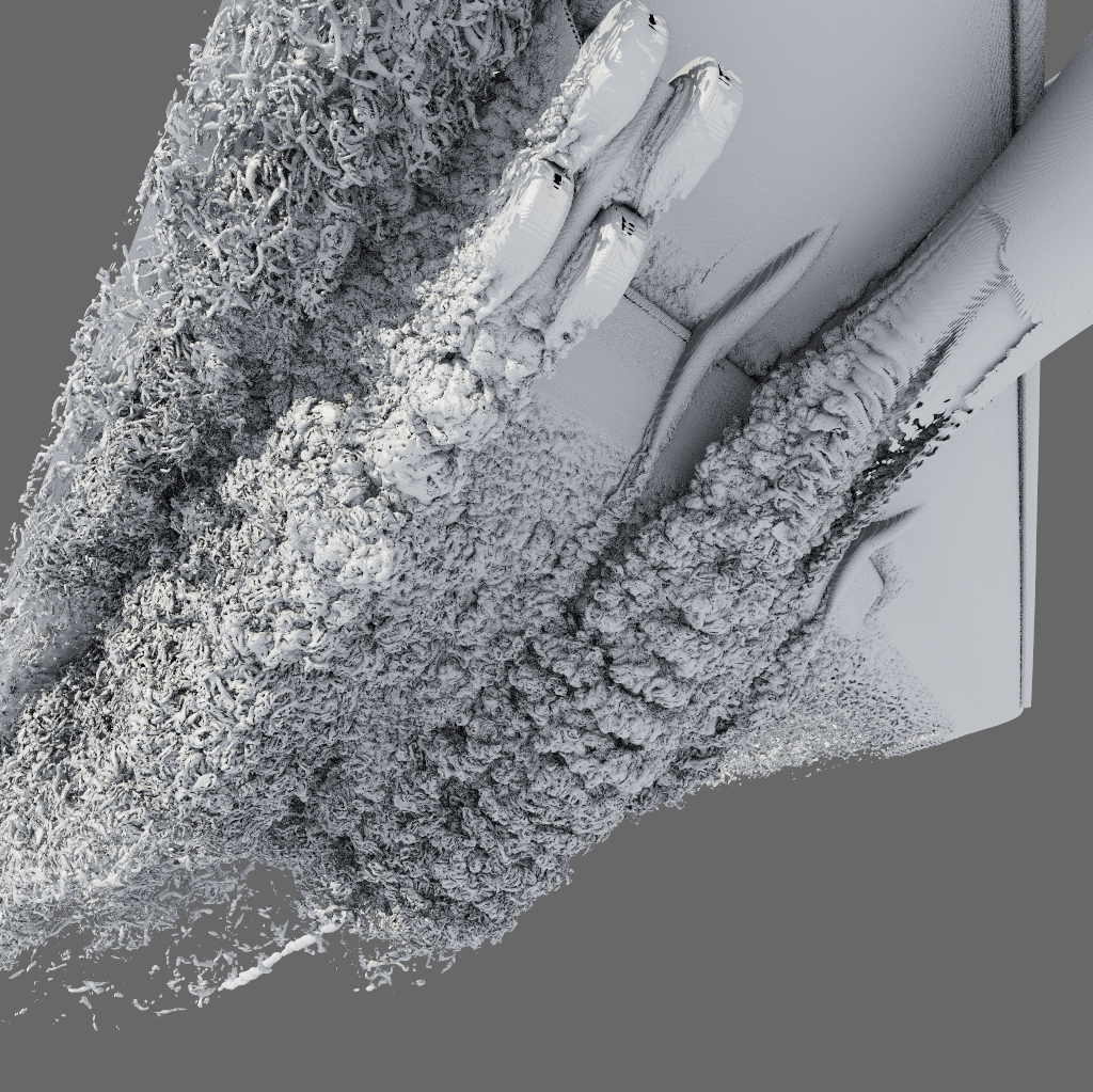 |
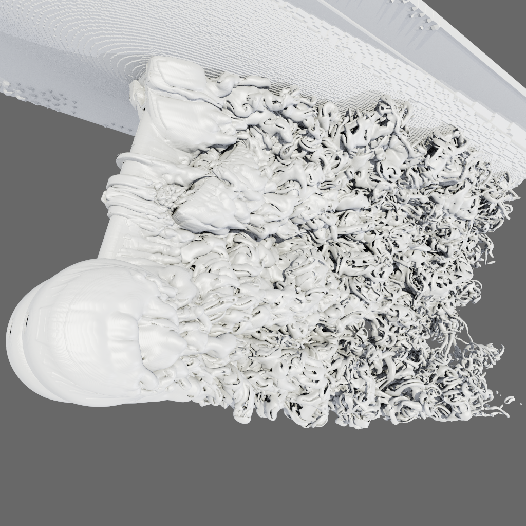
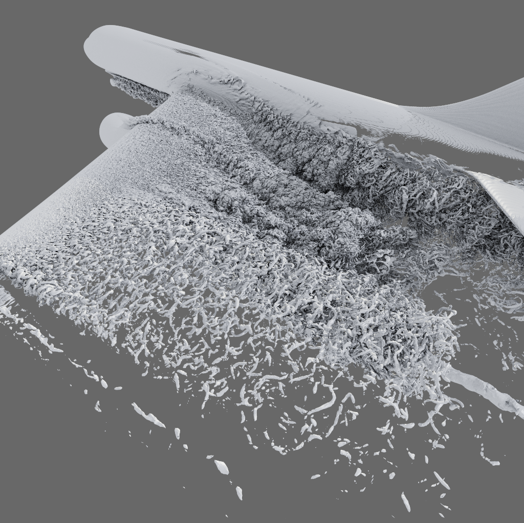
| TAC molecular cloud | NASA landing gear | NASA exajet | |
| (flash, block structured) | (LAVA, block structured) | Exa PowerFlow, Octree-AMR | |
| 5 levels, 392M cells | 13 levels, 249M cells | 4 levels, 626M cells | |
| field, | field, | field, | |
| 4M triangles, 1.1/2.6 sec | 52.7M triangles, 3.4/8.9 sec | 130M triangles, 8.4/22.2 sec | |
To demonstrate this application we implemented both our dual-cell generation and iso-surface extraction in CUDA. We split out code into the cell location kernel outlines above (Section 3.2), a kernel that executes the dual cell generation using this snapping kernel (Section 4), and a kernel that implements the MC case table for those duals that passed all tests. For the MC step, we used the case tables and edge tables from VTK [SAH00], and put those into CUDA _constant_ memory for fast access.
The kernel then takes the 8 vertices it is fed with, computes the 3D position at the center of each cell, and looks up the respective cell’s scalar values. Just like in the regular MC case the resulting 8 scalars are used to construct the case table index, which tells us which triangle vertices to construct on which edges of the hexahedron, and which triangles to emit. Obviously, when MC tags an edge for creating a vertex, we interpolate this vertex from the snapped positions, but otherwise there is no difference whatsoever; in fact, the code is an almost literal copy-and-paste from VTK’s implementation.
5.2 Generation of Output Triangle Mesh
Every time our CUDA kernel runs the MC step, it can produce up to 5 triangles. We use an atomic counter to append each such triangle to a buffer provided to our kernel, each time checking if the buffer is actually large enough. As the algorithm is completely deterministic, this means we can use exactly the same code both for counting how many triangles will eventually be generated, and for actually generating them: In a first pass, we execute the algorithm with a zero-sized outside buffer, which will not write any triangles, but modify the atomic to tell us how many would have been written. We then allocate an output buffer of that given size, reset the atomic, and simply run the same code again.
The result of this pass is a list of a “fat” triangle mesh where each triangle stores three comlete vertices. If desired, we then transform this to an indexed face set layout as follows: First, we tagging each vertex with an int specifying both the triangle it belongs to, and which of the triangle’s three vertices it is. We then sort this array of vertices by vertex position (using thrust::sort), which necessarily means that shared vertices will then be in adjacent locations.
Next, we execute a CUDA kernel that for each vertex in that sorted array, checks if that vertex has a predecessor at the same position, and returns if this is the case; otherwise, it assigns a unique index array position to this vertex by increasing another atomic counter, and writes the vertex to the final vertex array, and the index to the vertex’s relevant posiiton in the final index array, if such arrays have been provided. As above, we use the same trick of using the same kernel for both counting and final writing by simply passing null output arrays in the first pass, then allocating these arrays based on the atomic counter’s value, and re-run a second time with the actually allocated arrays.
Pseudo-code for this algorithm is given in Algorithm 4). Obviously, if one has an upper bound on the number of triangles respectively vertices generated the first of these passes can be omitted; as can be the entire generation of shared vertex array if a fat triangle layout is sufficient.
6 Results
To both validate and evaluate our algorithm we have implemented a variant using both CUDA and thrust (an earlier CPU variant used std::sort for sorting, std::lower_bound for binary search, and tbb for parallelization), and ran it on a workstation with a Intel i7-7820x CPU (8 cores, 3.6GHz), 64 GBs or RAM, SSDs, and a NVIDIA RTX 8000 GPU.
The models we used for testing are given in Figure 3, and span a wide range in both model complexity and formats. In particular, we point out that though Astro, Cloud, and Landing Gear have some sort of input mesh structure, the Exajet and impact data sets come as unsorted lists of individual AMR cells to which previous level-grid based approaches could not immediately be applied. Exajet also comes with “holes” in the sense that parts inside the airplane are not covered by any cells; using our method these will automatically be detected as model boundaries (even though some are inside the model), and handled correctly without any special effort.
As can be seen in the timings in Figure 3 our algorithm is not real-time, but still pretty fast, taking only a few seconds even for complex data sets with hundreds of millions of cells, and hundreds of millions of generated triangles.
7 Summary and Conclusion
In this paper, we have described an intriguingly simple technique for generating the dual mesh of an arbitrary cell-centered AMR data set that, though developed independently, may best be viewed as a simpler and somewhat more general re-formulation of the epsilon-box snapping method by Moran et al. In particular, the technique operates by “snapping” the right set of logical dual cells to actual AMR cells using a fast cell location kernel that itself operates solely on an array of sorted input cell coordinates. The method is intriguingly simple to implement, does not make any assumptions on input type or hierarchy structure, parallelizes trivially, lends itself well to efficient implementation on both CPU and GPU, and performs well even for highly non-trivial inputs.
Using this technique for generating dual cells we then demonstrated its application to the easy, fast, and parallel extraction of crack-free iso-surfaces; resulting in a framework that, using a CUDA implementation, can generate the iso-surface of even complex AMR data sets in seconds. Arguably the most defining trait of our approach is its simplicity that doesn’t requiring complex case tables, and works in all cases including data sets with “holes”, multiple level boundaries, etc. This simplicity not only facilitates simple code when implementing it, it also means that the algorithm is naturally parallel, and thus maps well to both multi-core CPUs and GPUs.
Future work.
In future, we would be very interested in seeing a implementation of this algorithm within VTK, and, in particular, within VTK-m [MSU∗16] (to which the algorithms parallel nature should lend very well), and to have it be used by actual end users of AMR software. Also, it would be interesting to see if our method could be integrated into an AMR volume ray tracing framework to generate an interpolant in the same way as originally done by Moran et al.
Acknowledgements
The Exajet data set is courtesy Pat Moran, NASA; the Landing Gear is courtesy Mike Barad (and others), NASA. TAC Molecular Cloud (“Cloud”) and Princeton Stellar Cluster Wind (“Wind”) are astrophysics simulations from the Theoretical Astrophysics Group in Cologne, and Princeton, respectively. LANL Deep Water Impact (“Impact”) is a simulation of an Asteroid Ocean Impact computed with xRage, and courtesy of Patchett et al.
We would also like to express our gratitude to Will Usher, Nate Morrical, Nate Marshak, Stefan Zellmann, Dave deMarle, Pat Moran, and Gunther Weber, for either help and/or fruitful discussions/feedback while working on this project: It is greatly appreciated!
References
- [BC89] Berger M. J., Colella P.: Local adaptive mesh refinement for shock hydrodynamics. Journal of Computational Physics 82, 1 (1989).
- [Bel10] Bell N.: High-Productivity CUDA Development with the Thrust Template Library, 2010.
- [BH12] Bell N., Hoberock J.: Thrust: A productivity-oriented library for CUDA. In GPU computing gems Jade edition. 2012.
- [BO84] Berger M. J., Oliger J.: Adaptive mesh refinement for hyperbolic partial differential equations. Journal of Computational Physics 53, 3 (1984).
- [CGL∗00] Colella P., Graves D., Ligocki T., Martin D., Modiano D., Serafini D., Van Straalen B.: Chombo software package for AMR applications design document, 2000.
- [CLP12] Carrard T., Law C., Pebay P.: A hyper tree grid implementation for AMR mesh manipulation and visualization in VTK. 21st International Meshing Roundtable, 2012.
- [FOR∗00] Fryxell B., Olson K., Ricker P., Timmes F. X., Zingale M., Lamb D. Q., MacNeice P., Rosner R., Truran J. W., Tufo H.: FLASH: An adaptive mesh hydrodynamics code for modeling astrophysical thermonuclear flashes. The Astrophysical Journal Supplement Series 131, 1 (2000).
- [GWC∗08] Gittings M., Weaver R., Clover M., Betlach T., Byrne N., Coker R., Dendy E., Hueckstaedt R., New K., R.Oakes W., Ranta D., Stefan R.: The RAGE radiation-hydrodynamic code. Computational Science & Discovery 1, 1 (2008).
- [KBH∗14] Kiris C. C., Barad M. F., Housman J. A., Sozer E., Brehm C., Moini-Yekta S.: The LAVA Computational Fluid Dynamics Solver. 52nd Aerospace Sciences Meeting, AIAA SciTech Forum 70 (2014).
- [LC87] Lorensen W. E., Cline H. E.: Marching Cubes: A High Resolution 3D Surface Construction Algorithm. In International Conference on Computer Graphics and Interactive Techniques (1987).
- [ME11] Moran P., Ellsworth D.: Visualization of AMR data with multi-level dual-mesh interpolation. IEEE transactions on visualization and computer graphics 17, 12 (2011), 1862–1871.
- [MMM14] Miller R., Moreland K., Ma K.-L.: Finely-Threaded History-Based Topology Computation. In Eurographics Symposium on Parallel Graphics and Visualization (2014).
- [MSU∗16] Moreland K., Sewell C., Usher W., Lo L.-t., Meredith J., Pugmire D., Kress J., Schroots H., Ma K.-L., Childs H., et al.: Vtk-m: Accelerating the visualization toolkit for massively threaded architectures. IEEE computer graphics and applications 36, 3 (2016).
- [Nie04] Nielson G. M.: Dual marching cubes. In IEEE Visualization 2004 (2004).
- [SAH00] Schroeder W. J., Avila L. S., Hoffman W.: Visualizing with VTK: a tutorial. IEEE Computer graphics and applications 20, 5 (2000).
- [SGLZ11] Sharkey K., Geveci B., Law C., Zagaris G.: Visualization & Analysis of AMR Datasets. published online, 2011.
- [SW04] Schaefer S., Warren J.: Dual marching cubes: Primal contouring of dual grids. In 12th Pacific Conference on Computer Graphics and Applications (2004).
- [WCM12] Weber G. H., Childs H., Meredith J. S.: Efficient parallel extraction of crack-free isosurfaces from adaptive mesh refinement (amr) data. In 2012 IEEE Symposium on Large Data Analysis and Visualization (2012).
- [WKL∗03] Weber G. H., Kreylos O., Ligocki T. J., Shalf J. M., Hagen H., Hamann B., Joy K. I.: Extraction of crack-free isosurfaces from adaptive mesh refinement data. In Hierarchical and Geometrical Methods in Scientific Visualization. 2003.
Appendix
Accompanying Sample Code
Sample CUDA code for the method described in this paper has been made available via github, on https://github.com/ingowald/cudaAmrIsoSurfaceExtraction.