What do you Mean?
The Role of the Mean Function in Bayesian Optimisation

Abstract.

Bayesian optimisation is a popular approach for optimising expensive black-box functions. The next location to be evaluated is selected via maximising an acquisition function that balances exploitation and exploration. Gaussian processes, the surrogate models of choice in Bayesian optimisation, are often used with a constant prior mean function equal to the arithmetic mean of the observed function values. We show that the rate of convergence can depend sensitively on the choice of mean function. We empirically investigate 8 mean functions (constant functions equal to the arithmetic mean, minimum, median and maximum of the observed function evaluations, linear, quadratic polynomials, random forests and RBF networks), using 10 synthetic test problems and two real-world problems, and using the Expected Improvement and Upper Confidence Bound acquisition functions.

We find that for design dimensions $\geq 5$ using a constant mean function equal to the worst observed quality value is consistently the best choice on the synthetic problems considered. We argue that this worst-observed-quality function promotes exploitation leading to more rapid convergence. However, for the real-world tasks the more complex mean functions capable of modelling the fitness landscape may be effective, although there is no clearly optimum choice.

1. Introduction

Bayesian optimisation (BO) is a popular approach for optimising expensive (in terms of time and/or money) black-box functions that have no closed-form expression or derivative information (Snoek et al., 2012; Shahriari et al., 2016). It is a surrogate-based modelling approach that employs a probabilistic model built with previous function evaluations. The Gaussian process (GP) model typically used in BO provides a posterior predictive distribution that models the target function in question and quantifies the amount of predictive uncertainty. A GP is a collection of random variables, any finite number of which have a joint Gaussian distribution (Rasmussen and Williams, 2006). It can be fully specified by its mean function and kernel function (also known as a covariance function) (Rasmussen and Williams, 2006). The kernel and mean functions may be regarded as specifying a Bayesian prior on the functions from which the data are generated. The kernel function describes the structure, such as the smoothness and amplitude, of the functions that can be modelled, while the mean function specifies the prior expected value of the function at any location (Shahriari et al., 2016).

In BO, the location that maximises an acquisition function (or infill criterion) is chosen as the next location to be expensively evaluated. Acquisition functions combine the surrogate model’s predictions and the uncertainty about its prediction to strike a balance between myopically exploiting areas of design space that are predicted to yield good-quality solutions and exploring regions that have high predicted uncertainty.

In the literature, many acquisition functions have been proposed in a number of works (Močkus et al., 1978; Srinivas et al., 2010; Hernández-Lobato et al., 2014; Wang and Jegelka, 2017; De Ath et al., 2019; Kushner, 1964), and, in general, no one strategy has been shown to be all-conquering due to the no free lunch theorem (Wolpert and Macready, 1997). However, recent works have shown that purely exploiting the surrogate model becomes a more effective strategy as the dimensionality of the problem increases (De Ath et al., 2019; Rehbach et al., 2020). Similarly, the role of the kernel function in BO has been investigated (Palar et al., 2020; Lindauer et al., 2019; Mukhopadhyay et al., 2017; Acar, 2013; Palar and Shimoyama, 2019). One of the most popular kernels is the radial basis function (also known as the squared exponential kernel) (Snoek et al., 2012). However, it is generally regarded as being too smooth for real-world functions (Stein, 2012; Rasmussen and Williams, 2006), and the Matérn family of kernels is often preferred.

Contrastingly, little attention has been paid to the role of the mean function in BO, with general practise being to use a constant value of zero (Wang and Jegelka, 2017; Hernández-Lobato et al., 2014; De Ath et al., 2019), although the constant value can also be inferred from the data (Shahriari et al., 2016). In general regression tasks, other mean functions have been considered, such as polynomials (Blight and Ott, 1975; Kennedy and O’Hagan, 2001; Williamson et al., 2015), and, more recently, non-parametric methods such as neural networks (Iwata and Ghahramani, 2017; Fortuin et al., 2019). In light of the lack of previous work into the role of the mean function in BO, we investigate the effect of different mean functions in BO in terms of both the convergence rate of the optimisation and quality of the best found solution. Specifically, we compare the performance of using different constant values, linear and quadratic functions, as well as using random forests and radial basis function networks.

Our main contributions can be summarised as follows:

• We provide the first empirical study of the effect of using different Gaussian process mean functions in Bayesian optimisation.

• We evaluate eight mean functions on ten well-known, synthetic test problems and two real-world applications. This assessment is on a range of design dimensions (2 to 10) and for two popular acquisition functions.

• We show empirically, and explain in terms of the exploration versus exploitation trade-off, that choosing the mean function to be the constant function equal to the worst-seen so far evaluation of the objective function is consistently no worse and often superior to other choices of mean function.

We begin in Section 2 by briefly reviewing Bayesian optimisation. In Section 3 we review Gaussian processes, paying particular attention to the mean function and introduce the various mean functions we evaluate in this work. Extensive empirical experimentation is carried out on well-known test problems and a two real-world applications in Section 4. We finish with concluding remarks in Section 5.

2. Bayesian Optimisation

Algorithm 1 Sequential Bayesian optimisation.

Inputs:

$M$	:	Number of initial samples
$T$	:	Budget on the number of expensive evaluations

1:Steps:

2:$X\leftarrow\operatorname{SpaceFillingSampling}(\mathcal{X},M)$ $\triangleright$ Initial samples

3:for $t=1\rightarrow M$ do

4:    $f_{t}\leftarrow f(\mathbf{x}_{t})$ $\triangleright$ Expensively evaluate all initial samples

5:$\mathcal{D}\leftarrow\{(\mathbf{x}_{t},f_{t})\}_{t=1}^{M}$

6:for $t=M+1\rightarrow T$ do

7:    $\boldsymbol{\theta}\leftarrow\text{Train$\mathcal{GP}$}(\mathcal{D})$ $\triangleright$ Train a GP model

8:    $\mathbf{x}^{\prime}\leftarrow\operatorname*{\arg\!\max}_{\mathbf{x}\in\mathcal{X}}~{}\alpha(\mathbf{x},\boldsymbol{\theta})$ $\triangleright$ Maximise infill criterion

9:    $f^{\prime}\leftarrow f(\mathbf{x}^{\prime})$ $\triangleright$ Expensively evaluate $\mathbf{x}^{\prime}$

10:    $\mathcal{D}\leftarrow\mathcal{D}\cup\{(\mathbf{x}^{\prime},f^{\prime})\}$ $\triangleright$ Augment training data

11:return $\mathcal{D}$

Bayesian optimisation (BO), also known as Efficient Global Optimisation (EGO), is a surrogate-assisted global search strategy that sequentially samples design space at likely locations of the global optimum, taking into account both the surrogate model’s prediction $\mu(\mathbf{x})$ and the associated prediction uncertainty $\sigma(\mathbf{x})$ (Jones et al., 1998). See (Shahriari et al., 2016; Brochu et al., 2010; Frazier, 2018) for comprehensive reviews of BO. Without loss of generality, we can define the problem of finding a global minimum of an unknown objective function $f:\mathbb{R}^{d}\mapsto\mathbb{R}$ as

(1) $$\min_{\mathbf{x}\in\mathcal{X}}f(\mathbf{x}),$$

where $\mathcal{X}\subset\mathbb{R}^{d}$ is the feasible design space of interest. We assume that $f$ is a black-box function, i.e. it has no simple closed form, but that we can have access the results of its evaluations $f(\mathbf{x})$ at any location $\mathbf{x}\in\mathcal{X}$, although evaluating $f(\mathbf{x})$ is expensive so that the number of evaluations required to locate the global optimum should be minimised.

Algorithm 1 outlines the BO procedure. It starts (line 2) with a space filling design, typically Latin hypercube sampling (McKay et al., 2000), of the feasible space. These samples $X=\{\mathbf{x}_{t}\}_{t=1}^{M}$ are then expensively evaluated with the function $f_{t}=f(\mathbf{x}_{t})$, and a training dataset $\mathcal{D}$ is constructed (line 5). Then, at each iteration of the sequential algorithm, a regression model, usually a Gaussian process ($\mathcal{GP}$), is constructed and trained (line 7) using the current training data. The choice of where next to expensively evaluate is determined by maximising an acquisition function (or infill criterion) $\alpha(\mathbf{x})$ which balances the exploitation of regions of design space that are predicted to yield good-quality solutions and exploration of regions of space where the predictive uncertainty is high. The design $\mathbf{x}^{\prime}$ maximising $\alpha(\mathbf{x})$ is expensively evaluated and the training data is subsequently augmented (lines 8 to 10). This process is then repeated until the budget has been expended.

Two of the most popular acquisition functions are Expected Improvement (EI) (Močkus et al., 1978) and Upper Confidence Bound (UCB) (Srinivas et al., 2010). EI measures the positive predicted improvement over the best solution evaluated thus far, $f^{\star}$:

(2) $$\alpha_{EI}(\mathbf{x})=\sigma(\mathbf{x})\left(s\Phi(s)+\phi(s)\right),$$

where $s=(f^{\star}-\mu(\mathbf{x}))/\sigma(\mathbf{x}))$ is the predicted improvement at $\mathbf{x}$ normalised by the uncertainty, and $\Phi(\cdot)$ and $\phi(\cdot)$ are the Gaussian cumulative density and probability density functions respectively. UCB is a weighted sum of the mean prediction and its associated uncertainty:

(3) $$\alpha_{UCB}(\mathbf{x})=-\left(\mu(\mathbf{x})-\sqrt{\beta_{t}}\sigma(\mathbf{x})\right),$$

where $\beta_{t}\geq 0$ is a weight that depends on the number of function evaluations $t$ and explicitly controls the exploitation vs. exploitation trade-off. Note that both EI and UCB are presented here in the form used for minimisation. While other acquisition functions have been proposed, such as probability of improvement (Kushner, 1964) and entropy-based methods such as predictive entropy search (Hernández-Lobato et al., 2014) and max-value entropy search (Wang and Jegelka, 2017), we limit our investigation to the commonly used EI and UCB to allow the focus on the mean functions themselves.

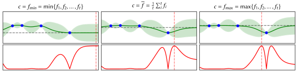
Figure 1. GP models with identical training data (blue) and kernel hyperparameters, along with different constant mean functions. The mean function used in each GP is shown (grey, dashed) and corresponds to the value of the smallest (left), arithmetic mean (centre), and largest (right) seen function values. The lower row shows the corresponding EI and its maximiser (red dashed). Note how the $\min$ and $\max$ models lead EI to prefer exploring and exploiting respectively.

3. Gaussian Processes

Gaussian processes are a common choice of surrogate model due to their strengths in uncertainty quantification and function approximation (Shahriari et al., 2016; Rasmussen and Williams, 2006). A GP is a collection of random variables, and any finite number of these have a joint Gaussian distribution (Rasmussen and Williams, 2006). We can define a Gaussian process prior over $f$ to be $\mathcal{GP}(m(\mathbf{x}),\kappa(\mathbf{x},\mathbf{x}^{\prime}\,|\,\boldsymbol{\theta}))$, where $m(\cdot)$ is the mean function and $\kappa(\cdot,\cdot\,|\,\boldsymbol{\theta})$ is the kernel function (covariance function) with hyperparameters $\boldsymbol{\theta}$. Given data consisting of $f$ evaluated at $t$ sampled locations $\mathcal{D}=\{(\mathbf{x}_{n},f_{n}\triangleq f(\mathbf{x}_{n}))\}_{n=1}^{t}$, the posterior distribution of $f$ at a given location $\mathbf{x}$ is Gaussian:

(4) $$p(f\,|\,\mathbf{x},\mathcal{D},\boldsymbol{\theta})=\mathcal{N}(f\,|\,\mu(\mathbf{x}),\sigma^{2}(\mathbf{x}))$$

with posterior mean and variance

(5) $$\mu(\mathbf{x}\,|\,\mathcal{D},\boldsymbol{\theta}) =m(\mathbf{x})+\boldsymbol{\kappa}(\mathbf{x},X)K^{-1}(\mathbf{f}-\mathbf{m})$$

(6) $$\sigma^{2}(\mathbf{x}\,|\,\mathcal{D},\boldsymbol{\theta}) =\kappa(\mathbf{x},\mathbf{x})-\boldsymbol{\kappa}(\mathbf{x},X)^{\top}K^{-1}\kappa(X,\mathbf{x}).$$

Here $X\in\mathbb{R}^{t\times d}$ is the matrix of design locations, $\mathbf{f}=\{f_{1},f_{2},\dots,f_{t}\}$ is the corresponding vector of true function evaluations and $\mathbf{m}=\{m(\mathbf{x}_{1}),m(\mathbf{x}_{1}),\dots,m(\mathbf{x}_{t})\}$ is the vector comprised of the mean function at the design locations. The kernel matrix $K\in\mathbb{R}^{t\times t}$ is given by $K_{ij}=\kappa(\mathbf{x}_{i},\mathbf{x}_{j}\,|\,\boldsymbol{\theta})$ and $\boldsymbol{\kappa}(\mathbf{x},X)$ is given by $[\boldsymbol{\kappa}(\mathbf{x},X)]_{i}=\kappa(\mathbf{x},\mathbf{x}_{i}\,|\,\boldsymbol{\theta})$. In this work we use an isotropic Matérn $5/2$ kernel:

(7) $$\kappa(\mathbf{x},\mathbf{x}^{\prime}\,|\,\boldsymbol{\theta})=\theta_{0}\left(1+\sqrt{5}r+\frac{5}{3}r^{2}\right)\exp\left(-\sqrt{5}r\right),$$

where $r=\theta_{1}\lVert\mathbf{x}-\mathbf{x}^{\prime}\rVert$ and $\boldsymbol{\theta}=[\theta_{0},\theta_{1}]$, as recommended for modelling realistic functions (Snoek et al., 2012). The kernel’s hyperparameters $\boldsymbol{\theta}$ are learnt via maximising the log marginal likelihood (up to a constant):

(8) $$\log p(\mathbf{f}\,|\,X,\boldsymbol{\theta})=-\frac{1}{2}\log\lvert K\rvert-\frac{1}{2}\left(\mathbf{f}-\mathbf{m}\right)^{\top}K^{-1}\left(\mathbf{f}-\mathbf{m}\right)$$

using a multi-restart strategy (Shahriari et al., 2016) with L-BFGS-B (Byrd et al., 1995). Henceforth, we drop the explicit dependencies on the data $\mathcal{D}$ and the kernel hyperparameters $\boldsymbol{\theta}$ for notational simplicity.

3.1. Mean Functions

It is well-known that the posterior prediction (4) of the GP reverts to the prior as the distance of $\mathbf{x}$ from the observed data increases, i.e. as $\min_{\mathbf{x}_{i}\in\mathcal{D}}\lVert\mathbf{x}-\mathbf{x}_{i}\rVert\rightarrow\infty$. In particular, the posterior mean reverts to the prior mean, i.e. $\mu(\mathbf{x})\approx m(\mathbf{x})$; and the posterior variance approaches the prior variance, $\theta_{0}$ for the Matérn kernel. The upper row of Figure 1 illustrates this effect for three different constant mean values: the best, average (arithmetic mean), and worst function values observed thus far. Note how the predicted values of the GP tend to the mean function (dashed) as the distance from the nearest evaluated location (blue) increases. The figure also shows another important, and often overlooked, aspect of the mean function: its effect on the acquisition function (lower). In this case three different locations maximise EI for the three mean functions, and it is not known a priori which location is preferable.

Practitioners of BO usually standardise the observations $f_{t}$ before fitting the GP at each iteration, i.e. they subtract the mean of the observations and divide by the standard deviation of the relevant feature/variable after which the mean function is taken as the constant function equal to zero; that is, the effective mean function is the constant function equal to the arithmetic mean of the observed function values. In addition, the prior variance of the GP is matched to the observed variance of the function values. Although the standardisation is not usually discussed in the literature, it is commonplace in standard BO libraries, e.g. GPyOpt (authors, 2016), BoTorch (Balandat et al., 2019) and Spearmint. It is, however, unclear whether this is the best choice for BO or whether a different mean function may be preferable. We now introduce the mean functions that will be evaluated in this work.

Here, we consider the mean function to be a set of basis functions $\mathbf{h}(\mathbf{x})$ with corresponding weights $\mathbf{w}$ (Rasmussen and Williams, 2006):

(9) $$m(\mathbf{x})=\mathbf{h}(\mathbf{x})^{\top}\mathbf{w}.$$

A constant mean function with value $c$, for example, can be written as $\mathbf{h}(\mathbf{x})=c\mathbf{1}$ with $\mathbf{w}=\mathbf{1}$. In addition to the standard constant function equal to the arithmetic mean of the data $c=\bar{f}=t^{-1}\sum_{i}^{t}f_{i}$, we consider three other constant values: using the best and worst seen observation’s value at each iteration, i.e. $c=f_{min}=f^{\star}=\min\{f_{1},f_{2},\dots,f_{t}\}$ and $c=f_{max}=\max\{f_{1},f_{2},\dots,f_{t}\}$, and the median observed value $c=f_{med}=\operatorname*{median}\{f_{1},f_{2},\dots,f_{t}\}$. In comparison to using the data mean $c=\bar{f}$, using $c=f_{min}$ leads to acquisition functions becoming more exploratory, as illustrated in Figure 1 (left panel). This is because locations far away from previously evaluated solutions $\mathcal{D}$ will have predicted means $\mu(\mathbf{x})$ equal to the $f^{\star}$ and with large predicted uncertainty, leading to large values of, for example, EI and UCB. Conversely, using $c=f_{max}$ will, as illustrated in Figure 1 (right panel), lead to increased exploitation due to regions far from $\mathcal{D}$ having large uncertainty, but poor predicted values and hence small $\alpha(\mathbf{x})$. Interestingly, the effect of using $c=\bar{f}$ or $c=f_{med}$ will change over the course of the optimisation. When there are relatively few function evaluations $\bar{f}$ and $f_{med}$ will be approximately $(f_{min}+f_{max})/2$. However, as the number of expensive function evaluations increases and the optimisation converges towards the (estimated) optimum, $\bar{f}$ and particularly $f_{med}$ will tend to approach $f_{min}$, thus leading to increased exploration.

We also consider linear and quadratic mean functions. Linear mean functions are defined as $\mathbf{h}(\mathbf{x})=[1,x^{(1)},x^{(2)},\dots,x^{(d)}]$, with corresponding weights $\mathbf{w}\in\mathbb{R}^{d+1}$ and where $x^{(i)}$ refers to the $i$th element of $\mathbf{x}$. Quadratic mean functions are defined similarly, with polynomial terms up to degree $2$ and with weights $\mathbf{w}\in\mathbb{R}^{q}$, where $q=\binom{d+2}{d}$. To avoid overfitting to the data, these regressions are typically trained via a regularised least-squares approximation, i.e. ridge regression (also known as Tikhonov regularization). The optimal regularised weights $\mathbf{w}^{*}$ are estimated by solving

(10) $$\mathbf{w}^{*}=\operatorname*{\arg\!\min}_{\mathbf{w}}\,\lVert\mathbf{f}-H\mathbf{w}\rVert^{2}+\lambda\lVert\mathbf{w}\rVert^{2},$$

where $H=[\mathbf{h}(\mathbf{x}_{1}),\mathbf{h}(\mathbf{x}_{2}),\dots,\mathbf{h}(\mathbf{x}_{t})]$ and $\lambda\geq 0$ controls the amount of regularisation. The ordinary least squares estimator is

(11) $$\mathbf{w}^{*}=\left(H^{\top}H+\lambda\mathbf{I}\right)^{-1}H^{\top}\mathbf{f},$$

In this work, the regularisation parameter $\lambda$ was chosen via five-fold cross-validation for $\lambda\in\{10^{-6},10^{-5},\dots,10^{1},10^{2}\}$.

Another choice of basis functions are radial basis functions (RBFs), which have the property that each basis function only depends on the Euclidean distance from a fixed centre (Bishop, 2006). These are known as RBF networks and can be thought of as either linear neural networks using RBF activation functions (Orr, 1996) or as finite-dimensional Gaussian processes (Bishop, 2006). A commonly used set of basis functions, and the ones used in this work, are the Gaussian RBFs $\phi_{i}(\mathbf{x})=\exp(-\gamma\lVert\mathbf{x}-\mathbf{z}_{i}\rVert)$. While any set of locations can be used as the centres $\mathbf{z}_{i}$, we place a Gaussian RBF at each of the previously-evaluated locations, i.e. $\mathbf{z}_{i}\equiv\mathbf{x}_{i}~{}\forall i=1,\ldots,t$, resulting in $\mathbf{h}(\mathbf{x})=[\phi_{1}(\mathbf{x}),\phi_{2}(\mathbf{x}),\dots,\phi_{t}(\mathbf{x})]$. Similarly to the linear and quadratic mean functions, the regularisation parameter $\lambda$ and length scale $\gamma$ were chosen via five-fold cross validation. Values of $\lambda$ were selected in the same range as for the linear and quadratic mean functions, and the values of $\gamma$ were selected from $\gamma\in\{10^{-3},10^{-2.5},\dots,10^{1.5},10^{2}\}$. A more fine-grained selection of values were chosen following a preliminary investigation which revealed the modelling error to be more sensitive to changes in $\gamma$ than $\lambda$. We note here that the use of regularisation is particularly important when placing an RBF on each evaluated location because the RBF network will otherwise be able to perfectly interpolate the data. This would lead to $\mathbf{f}\equiv\mathbf{m}$ and therefore (8) would reduce to $-\tfrac{1}{2}\log\lvert K\rvert$, which can be maximised by either $\theta_{0}\rightarrow 0$ or $\theta_{1}\rightarrow\infty$ in (7). This results in the posterior variance estimates $\sigma^{2}(\mathbf{x})$ being over-confident and thus having small variance everywhere with predictions determined by the mean function.

Lastly, we include a non-parametric regressor, extremely randomised trees, better known as Extra-Trees (ET, (Geurts et al., 2006)), a variant of Random Forests (RF, (Breiman, 2001)). RFs are ensembles of classification or regression trees that are each trained on a different randomly chosen subsets of the data. Unlike RFs, that attempt to split the data at each cut-point of a tree optimally, the ET method instead selects the cut-point as the best from a small set of randomly chosen cut-points; this additional randomisation results in a smoother regression in comparison to RFs. Given that ETs use randomised cut-points, they typically use all the training data in each tree. However, to counteract the overfitting that this will produce, we allow each item in the training set to be resampled, instead of using all elements of the set for each tree. Note that, while not presented as such here, RFs can also be interpreted as a kernel method (Scornet, 2016; Davies and Ghahramani, 2014).

4. Experimental Evaluation

We now investigate the performance of the mean functions discussed in Section 3.1 using the EI and UCB acquisition functions (Section 2) on ten well-known benchmark functions with a range dimensionality and landscape properties, and two real-world applications. Full results of all experimental evaluations are available in the supplementary material. The mean functions to be evaluated are the constant functions, $c=\bar{f}$, $c=f_{med}$, $c=f_{min}$, and $c=f_{max}$, labelled Arithmetic, Median, Min, and Max respectively, as well as the Linear, Quadratic, Extra-Trees (RandomForest), and RBF network-based (RBF) mean functions.

A Gaussian process surrogate model with an isotropic Matérn $5/2$ kernel (7) was used in all experiments. The Bayesian optimisation runs themselves were carried out as in Algorithm 1, with the additional step of fitting a mean function before training the GP (Algorithm 1, line 7) at each iteration. All test problems evaluated in this work were scaled to $[0,1]^{d}$, and observations were standardised at each BO iteration, prior to mean function fitting. The models were initially trained on $M=2d$ observations generated by maximin Latin hypercube sampling (McKay et al., 2000), and each optimisation run was repeated $51$ times with different initialisation. The same set of $51$ initial observations were used for each of the mean functions to enable statistical comparisons. The hyperparameters $\boldsymbol{\theta}$ of the GP were optimised by maximising the marginal log likelihood (8) with L-BFGS-B (Byrd et al., 1995) using 10 restarts. Following common practise, maximisation of the acquisition functions was carried out via multi-start optimisation; details of the full procedure can be found in (Balandat et al., 2019). The trade-off between exploitation and exploration in UCB, $\beta_{t}$, is set to Theorem 1 in (Srinivas et al., 2010), which increases logarithmically with the number of function evaluations, with $\sqrt{\beta_{t}}$ approximately in the range $[3,6]$. The Bayesian optimisation pipeline and mean functions were implemented with BoTorch (Balandat et al., 2019) and code is available online to recreate all experiments, as well as the LHS initialisations used and full optimisation runs.

Optimisation quality is measured with simple regret $R_{t}$, which is the difference between the true minimum value $f(\mathbf{x}^{*})$ and the best value found so far after $t$ evaluations:

(12) $$R_{t}=|f(\mathbf{x}^{*})-\min\{f_{1},f_{2},\dots,f_{t}\}|.$$

4.1. Synthetic Experiments

Name	$d$		Name	$d$
Branin	2		Ackley	5
Eggholder	2		Hartmann6	6
GoldsteinPrice	2		Michalewicz	10
SixHumpCamel	2		Rosenbrock	10
Shekel	4		StyblinskiTang	10

Table 1. Synthetic functions used and their dimensionality $d$. Formulae for all functions can be found at http://www.sfu.ca/~ssurjano/optimization.html.

The mean functions were evaluated on the ten popular synthetic benchmark functions listed in Table 1 with a budget of $200$ function evaluations that included the initial $2d$ LHS samples. These functions were selected due to their different dimensionality and landscape properties, such the presence of multiple local or global minima (Ackley, Eggholder, Hartmann6, GoldsteinPrice, StyblinskiTang, Shekel) deep, valley-like regions (Branin, Rosenbrock, SixHumpCamel), and steep ridges and drops (Michalewicz).

Table 2. Mean function performance using the EI acquisition function. Median regret (column left) and median absolute deviation from the median (MAD, column right) after 200 function evaluations across the 51 runs. The method with the lowest median performance is shown in dark grey, with those statistically equivalent shown in light grey.

Mean function	Branin (2)		Eggholder (2)		GoldsteinPrice (2)		SixHumpCamel (2)		Shekel (4)
	Median	MAD	Median	MAD	Median	MAD	Median	MAD	Median	MAD
Arithmetic	$1.35\text{\times}{10}^{-05}$	$1.82\text{\times}{10}^{-05}$	$1.58\text{\times}{10}^{00}$	$1.93\text{\times}{10}^{00}$	$4.18\text{\times}{10}^{-02}$	$5.32\text{\times}{10}^{-02}$	$2.51\text{\times}{10}^{-05}$	$2.58\text{\times}{10}^{-05}$	$8.13\text{\times}{10}^{-02}$	$1.19\text{\times}{10}^{-01}$
Median	$9.35\text{\times}{10}^{-06}$	$1.17\text{\times}{10}^{-05}$	$3.02\text{\times}{10}^{00}$	$2.67\text{\times}{10}^{00}$	$5.03\text{\times}{10}^{-02}$	$5.59\text{\times}{10}^{-02}$	$1.40\text{\times}{10}^{-05}$	$1.49\text{\times}{10}^{-05}$	$1.54\text{\times}{10}^{-01}$	$2.24\text{\times}{10}^{-01}$
Min	$1.18\text{\times}{10}^{-05}$	$1.31\text{\times}{10}^{-05}$	$2.82\text{\times}{10}^{00}$	$3.13\text{\times}{10}^{00}$	$6.25\text{\times}{10}^{-02}$	$8.03\text{\times}{10}^{-02}$	$2.25\text{\times}{10}^{-05}$	$2.29\text{\times}{10}^{-05}$	$7.02\text{\times}{10}^{00}$	$9.75\text{\times}{10}^{-01}$
Max	$7.21\text{\times}{10}^{-06}$	$8.81\text{\times}{10}^{-06}$	$2.69\text{\times}{10}^{00}$	$2.48\text{\times}{10}^{00}$	$6.87\text{\times}{10}^{-02}$	$7.40\text{\times}{10}^{-02}$	$1.52\text{\times}{10}^{-05}$	$1.84\text{\times}{10}^{-05}$	$7.16\text{\times}{10}^{-02}$	$1.05\text{\times}{10}^{-01}$
Linear	$5.13\text{\times}{10}^{-06}$	$5.58\text{\times}{10}^{-06}$	$2.82\text{\times}{10}^{00}$	$2.85\text{\times}{10}^{00}$	$1.05\text{\times}{10}^{-01}$	$1.19\text{\times}{10}^{-01}$	$7.98\text{\times}{10}^{-06}$	$8.14\text{\times}{10}^{-06}$	$6.47\text{\times}{10}^{00}$	$1.57\text{\times}{10}^{00}$
Quadratic	$1.05\text{\times}{10}^{-05}$	$1.09\text{\times}{10}^{-05}$	$3.59\text{\times}{10}^{00}$	$4.03\text{\times}{10}^{00}$	$5.55\text{\times}{10}^{-02}$	$6.03\text{\times}{10}^{-02}$	$6.27\text{\times}{10}^{-06}$	$6.52\text{\times}{10}^{-06}$	$6.47\text{\times}{10}^{00}$	$1.30\text{\times}{10}^{00}$
RandomForest	$5.35\text{\times}{10}^{-04}$	$4.86\text{\times}{10}^{-04}$	$3.93\text{\times}{10}^{00}$	$4.22\text{\times}{10}^{00}$	$2.41\text{\times}{10}^{00}$	$2.14\text{\times}{10}^{00}$	$2.96\text{\times}{10}^{-04}$	$3.56\text{\times}{10}^{-04}$	$2.84\text{\times}{10}^{00}$	$2.76\text{\times}{10}^{00}$
RBF	$1.36\text{\times}{10}^{-04}$	$1.07\text{\times}{10}^{-04}$	$3.27\text{\times}{10}^{00}$	$3.45\text{\times}{10}^{00}$	$1.76\text{\times}{10}^{00}$	$2.39\text{\times}{10}^{00}$	$3.76\text{\times}{10}^{-05}$	$4.63\text{\times}{10}^{-05}$	$7.95\text{\times}{10}^{00}$	$1.05\text{\times}{10}^{00}$
Mean function	Ackley (5)		Hartmann6 (6)		Michalewicz (10)		Rosenbrock (10)		StyblinskiTang (10)
	Median	MAD	Median	MAD	Median	MAD	Median	MAD	Median	MAD
Arithmetic	$4.27\text{\times}{10}^{00}$	$6.06\text{\times}{10}^{00}$	$4.00\text{\times}{10}^{-03}$	$5.46\text{\times}{10}^{-03}$	$7.22\text{\times}{10}^{-02}$	$1.03\text{\times}{10}^{-01}$	$8.38\text{\times}{10}^{02}$	$3.27\text{\times}{10}^{02}$	$6.47\text{\times}{10}^{01}$	$2.58\text{\times}{10}^{01}$
Median	$2.10\text{\times}{10}^{00}$	$2.06\text{\times}{10}^{00}$	$8.31\text{\times}{10}^{-04}$	$1.02\text{\times}{10}^{-03}$	$7.88\text{\times}{10}^{-02}$	$1.12\text{\times}{10}^{-01}$	$7.14\text{\times}{10}^{02}$	$2.78\text{\times}{10}^{02}$	$6.72\text{\times}{10}^{01}$	$2.49\text{\times}{10}^{01}$
Min	$4.64\text{\times}{10}^{00}$	$9.59\text{\times}{10}^{-01}$	$3.27\text{\times}{10}^{-03}$	$3.72\text{\times}{10}^{-03}$	$1.39\text{\times}{10}^{00}$	$7.49\text{\times}{10}^{-01}$	$7.00\text{\times}{10}^{02}$	$2.21\text{\times}{10}^{02}$	$8.15\text{\times}{10}^{01}$	$2.78\text{\times}{10}^{01}$
Max	$1.66\text{\times}{10}^{00}$	$1.23\text{\times}{10}^{00}$	$7.47\text{\times}{10}^{-04}$	$9.88\text{\times}{10}^{-04}$	$2.75\text{\times}{10}^{-02}$	$3.72\text{\times}{10}^{-02}$	$6.95\text{\times}{10}^{02}$	$3.64\text{\times}{10}^{02}$	$2.84\text{\times}{10}^{01}$	$2.08\text{\times}{10}^{01}$
Linear	$1.65\text{\times}{10}^{01}$	$2.42\text{\times}{10}^{00}$	$1.21\text{\times}{10}^{-02}$	$1.32\text{\times}{10}^{-02}$	$1.30\text{\times}{10}^{00}$	$8.55\text{\times}{10}^{-01}$	$1.93\text{\times}{10}^{03}$	$1.02\text{\times}{10}^{03}$	$1.10\text{\times}{10}^{02}$	$2.99\text{\times}{10}^{01}$
Quadratic	$9.83\text{\times}{10}^{00}$	$5.81\text{\times}{10}^{00}$	$9.95\text{\times}{10}^{-03}$	$9.63\text{\times}{10}^{-03}$	$1.03\text{\times}{10}^{00}$	$6.84\text{\times}{10}^{-01}$	$1.81\text{\times}{10}^{03}$	$8.90\text{\times}{10}^{02}$	$8.58\text{\times}{10}^{01}$	$4.14\text{\times}{10}^{01}$
RandomForest	$5.16\text{\times}{10}^{00}$	$7.70\text{\times}{10}^{-01}$	$8.12\text{\times}{10}^{-02}$	$5.63\text{\times}{10}^{-02}$	$1.25\text{\times}{10}^{-01}$	$1.43\text{\times}{10}^{-01}$	$4.21\text{\times}{10}^{03}$	$2.29\text{\times}{10}^{03}$	$7.27\text{\times}{10}^{01}$	$1.78\text{\times}{10}^{01}$
RBF	$7.90\text{\times}{10}^{00}$	$1.94\text{\times}{10}^{00}$	$2.75\text{\times}{10}^{-01}$	$1.55\text{\times}{10}^{-01}$	$9.05\text{\times}{10}^{-01}$	$5.57\text{\times}{10}^{-01}$	$2.73\text{\times}{10}^{03}$	$1.32\text{\times}{10}^{03}$	$1.17\text{\times}{10}^{02}$	$2.86\text{\times}{10}^{01}$

Table 2 shows the median regret over the 51 repeated experiments, together with the median absolute deviation from the median (MAD) for the mean functions using the EI acquisition function. Due to space constraints, the corresponding table for UCB is included in the supplementary material. The method with the lowest (best) median regret on each function is highlighted in dark grey, and those highlighted in light grey are statistically equivalent to the best method according to a one-sided paired Wilcoxon signed-rank test (Knowles et al., 2006) with Holm-Bonferroni correction (Holm, 1979) ($p\geq 0.05$).

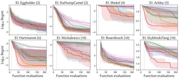
Figure 2. Illustrative convergence plots for eight benchmark problems using the EI acquisition function. Each plot shows the median regret, with shading representing the interquartile range across the 51 runs and the dashed vertical line indicating the end of the initial LHS phase.

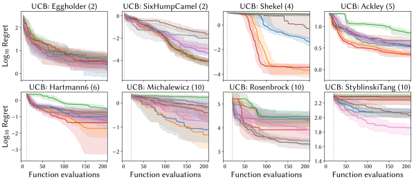
Figure 3. Illustrative convergence plots for eight benchmark problems using the UCB acquisition function. Each plot shows the median regret, with shading representing the interquartile range across the 51 runs and the dashed vertical line indicating the end of the initial LHS phase.

The convergence of the various mean functions on $8$ illustrative test problems are shown using the EI (Figure 2) and UCB (Figure 3) acquisition functions. Convergence plots for the Branin and GoldsteinPrice test problems were visually similar to Eggholder and SixHumpCamel respectively; they are available in the supplementary material. As one might expect, because points are naturally less distant from one another, the choice of mean function has less impact in 2 dimensions. Although, interestingly, optimisation runs with the UCB algorithm in $d=2$ achieve lower regret with the constant mean functions compared to the others evaluated.

Perhaps surprisingly, the non-constant mean functions, Linear, Quadratic, RandomForest and RBF, appear to offer no advantage over the constant mean functions despite their ability to model the large scale optimisation landscape. The Quadratic model, in two dimensions where there are only three parameters to be fitted, appears to be well suited to the SixHumpCamel function which is roughly bowl-shaped (albeit with quartic terms); however, this appears to be an exceptional case.

In higher dimensions with the EI acquisition function, using the worst observation value as the constant mean function (Max) consistently provides the lowest regret on the test functions evaluated. This is consistent with recent work (De Ath et al., 2019; Rehbach et al., 2020) showing that being more exploitative in higher dimensions is preferable to most other strategies. However, for the UCB acquisition function this is not the case and no mean function is consistently best. We suspect that this is because the value of $\beta_{t}$ is so large that the UCB function (3) is always dominated by the exploratory term ($\sqrt{\beta_{t}}\sigma(\mathbf{x})$) so that the mean function has relatively little influence. This is in contrast to EI, which has been shown (De Ath et al., 2019) to be far more exploitative than UCB.

The standard choice of using a constant mean function equal to $\bar{f}$ the arithmetic mean of the observations (Arithmetic) is, in higher dimensions ($d\geq 5$), only statistically equivalent to the best-performing method on one of the five test functions for both EI and UCB. This result calls into question the efficacy of the common practise of using the $\bar{f}$ constant mean function in all Bayesian optimisation tasks. Based on these results we suggest that an increase performance may be obtained by using the Max mean function with EI. Although there does not appear to be such a clear-cut answer as to which mean function should be used in conjunction with the UCB acquisition function, we posit that this is less important because, based on these optimisation results, one would prefer the performance of EI over UCB in general.

4.2. Active Learning for Robot Pushing

Like (Wang and Jegelka, 2017; Jiang et al., 2019; De Ath et al., 2019, 2020) we optimise the control parameters for two active learning robot pushing problems (Wang et al., 2018); see (De Ath et al., 2019) for a diagrammatic outline of the problems. In the $d=4$ push4 problem, a robot should push an object towards an unknown target location and is constrained such that it can only travel in the initial direction of the object. Once the robot has finished pushing, it receives feedback in the form of the object-target distance. The robot is parametrised by its initial location, the orientation of its pushing hand and how long it pushes for. This can therefore be cast as a minimisation problem in which the four parameter values are optimised with respect to the object’s final distance from the target. The object’s initial location is fixed to the centre of the problem domain (Wang and Jegelka, 2017) and the target location is changed for each of the 51 optimisation runs, with these kept the same across mean functions. Thus, the optimisation performance is considered over problem instances rather initialisations of a single instance.

The second problem, push8, two robots push their respective objects towards two unknown targets, with their movements constrained so that they always travel in the direction of their object’s initial location. The $d=8$ parameters controlling the robots can be optimised to minimise the summed final object-target distances. Like push4, initial object locations were fixed for problem instances and the targets’ locations were chosen randomly, with a constraint enforcing that both objects could cover the targets without overlapping. This means, however, that in some problem instances it may not be possible for both robots to push their objects to their respective targets because they will block each other. Thus, for push8 we report the final summed object-distances rather than the regret due to the global optimum not being known.

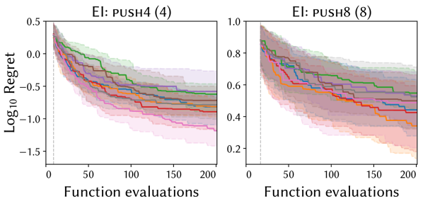
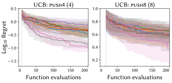
Figure 4. Convergence plots for the robot pushing problem using EI and UCB. Each plot shows the median regret, with shading representing the interquartile range of the 51 runs.

Figure 4 shows the convergence plots using the various mean functions with the EI and UCB acquisition functions. Tabulated results are available in the supplementary material. In the four-dimensional push4 problem, one of the worst-performing mean functions on the synthetic functions, RandomForest, had substantially lower regret than the other mean functions using UCB on both problems and for EI on push4. However, in the eight-dimensional push8, all mean functions were statistically equivalent when using EI, apart from Min, Linear and RBF, which were worse. However, when using UCB, the RandomForest mean function was statistically better than all other mean functions, and it achieved results comparable to using EI.

It might be suspected that the superior ability of the Random Forest (and RBF on some problems) to represent the inherently difficult landscape features of these problems would account for the better performance of RandomForest. The landscape for these problems has sharp changes (high gradients) in the function, e.g. when a change of the robot’s starting location results in the object no longer being pushed towards the target, as well as plateaux where changes in certain parameter values have little effect, e.g. if the amount of pushing time results in the robot not reaching the object. However, we investigated the mean prediction error of each of the combined mean plus Gaussian process models trained on the first 100 expensively evaluated locations by calculating the normalised root mean squared prediction error at 1000 locations (chosen by Latin Hypercube Sampling). As shown in the supplementary material, this indicates that, in fact, the RF model has a comparatively poor prediction error. By contrast, the RBF mean function yields the most accurate model of the overall landscape, but it only shows better performance for push4 using UCB. These prediction errors were evaluated over the entire domain and, therefore, it is possible that the RF mean function is sufficiently superior in the vicinity of the optimum to allow the more rapid convergence seen here.

Interestingly, the performance of the Max mean function with EI on the synthetic test problems is not reflected on these two more real-world problems. However, both the Arithmetic and Max mean functions are statistically equivalent on both push4 and push8, with Max having lower median regret and MAD than Arithmetic. Nonetheless, it remains unclear why the RF mean function gives best performance in three of these four cases.

4.3. Pipe Shape Optimisation

Lastly, we evaluate the mean functions on a real-world computational fluid dynamics (CFD) optimisation problem. The goal of the PitzDaily CFD problem (Daniels et al., 2018) is to minimise the pressure loss between a pipe’s entrance (inflow) and exit (outflow) by optimising the shape of the pipe’s lower wall. The loss is evaluated by generating a CFD mesh and simulating the two-dimensional flow using OpenFOAM (Jasak et al., 2007), with each function evaluation taking between $60$ and $90$ seconds. The decision variables in the problem are the control points of a Catmull-Clark subdivision curve that represents the lower wall’s shape; see (Daniels et al., 2018) for a pictorial representation of these. In this work we use $5$ control points, resulting in a 10-dimensional decision vector. The control points are constrained to lie in a polygon, rather than a hypercube for all previous problems, and, therefore, we draw initial samples uniformly from within the constrained region rather than using LHS. Similarly, we use CMA-ES (Hansen, 2009) to optimise the acquisition functions and penalise locations that violate the constraints.

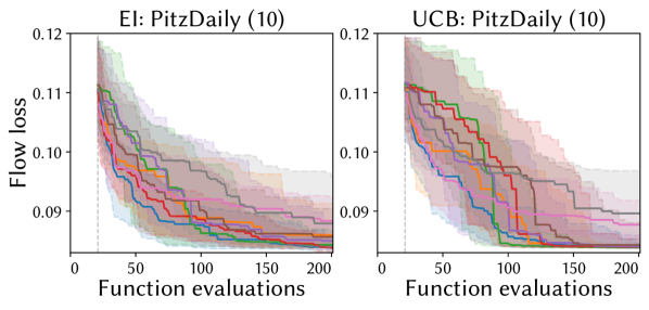
Figure 5. Convergence plots for the PitzDaily test problem using EI and UCB. Each plot shows the median regret, with shading representing the interquartile range of the 51 runs.

Convergence plots of the flow loss for the mean functions with EI and UCB are shown in Figure 5. The Arithmetic, Min and Max constant mean functions, when using EI, are all statistically equivalent and the best-performing. It is interesting to note the contrasting performance between the RandomForest mean function on this and the robot pushing tasks.

As shown in Figure 5, using the UCB acquisition function leads to the constant mean and Linear mean functions all having a median flow loss within $10^{-4}$ of one another, with their inter-quartile ranges rapidly decreasing. This effect can also be seen towards the end of the optimisation runs with EI. Inspection of solutions (control points) with a flow loss $\approx 0.084$ revealed that they all had distinct values but that they led to very similar sub-division curves. This implies that they all represented essentially the same inner wall shape and thus indicate the presence of either one large, valley-like global optimum or many, global optima. We suggest that this may be the actual minimum flow loss achievable for this problem. All mean functions, in combination with both EI and UCB, were able to successfully discover solutions that led to a flow loss of less than $0.0903$ found by a local, gradient-based method in (Nilsson et al., 2014) that used approximately 500 function evaluations. This highlights the strength of Bayesian optimisation in general because the convergence rates shown in Figure 5 are far more rapid for the majority of mean functions and realise better solutions than the local, adjoint method.

5. Conclusion

We have investigated the effect of using different prior mean functions in the Gaussian process model during Bayesian optimisation when using the expected improvement and upper confidence bound acquisition functions. This was assessed by performing BO on ten synthetic functions and two real-world problems. The constant mean function Max, which uses a constant value of the worst-seen expensive function evaluation thus far, was found to consistently out-perform the other mean functions across the synthetic functions in higher dimensions, and was statistically equivalent to the best performing mean function on nine out of ten functions. We suggest that this is because this mean function tends to promote exploitation which can lead to rapid convergence in higher dimensions (De Ath et al., 2019; Rehbach et al., 2020) because exploration is implicitly provided through the necessarily inaccurate surrogate modelling. However, on the two, real-world problems this trend did not continue, but its performance was still statistically equivalent to the commonly-used mean equal to the arithmetic mean of the observations. For this reason we recommend using the Max mean function in conjunction with expected improvement for, at worst, the same performance as a zero mean and generally improved performance in higher dimensions.

Interestingly, the lack of consistency between mean function performance on the synthetic and real-world problems may indicate a larger issue in BO, namely that synthetic benchmarks do not always contain the same types of functional landscapes as real-world problems. In future work we would like to characterise a function’s landscape during the optimisation procedure and adaptively select the best-performing components of the BO pipeline, e.g. mean function, kernel, and acquisition function, to suit the problem structure.

This work focused on learning a mean function independent of the training of the GP. In further work we would like to jointly learn the parameters of the mean function, i.e. the weights in (9), alongside the hyperparameters of the GP itself. The efficacy of the BO approach clearly depends crucially on the ability of the surrogate model to accurately predict the function’s value in unvisited locations. We therefore look forward to evaluating a fully-Bayesian approach that marginalises over the mean function parameters and kernel hyperparameters. Although the Monte Carlo sampling required to evaluate the resulting acquisition functions may be substantial, an important area of investigation is whether fully-Bayesian models can significantly improve the convergence of Bayesian Optimisation.

- (1)
- Acar (2013) Erdem Acar. 2013. Effects of the correlation model, the trend model, and the number of training points on the accuracy of Kriging metamodels. Expert Systems 30, 5 (2013), 418–428.
- authors (2016) The GPyOpt authors. 2016. GPyOpt: A Bayesian Optimization framework in python. http://github.com/SheffieldML/GPyOpt.
- Balandat et al. (2019) Maximilian Balandat, Brian Karrer, Daniel R. Jiang, Samuel Daulton, Benjamin Letham, Andrew Gordon Wilson, and Eytan Bakshy. 2019. BoTorch: Programmable Bayesian Optimization in PyTorch. arXiv:1910.06403
- Bishop (2006) Christopher M. Bishop. 2006. Pattern Recognition and Machine Learning. Springer, Berlin, Heidelberg.
- Blight and Ott (1975) B. J. N. Blight and L. Ott. 1975. A Bayesian approach to model inadequacy for polynomial regression. Biometrika 62, 1 (1975), 79–88.
- Breiman (2001) Leo Breiman. 2001. Random Forests. Machine Learning 45, 1 (2001), 5––32.
- Brochu et al. (2010) Eric Brochu, Vlad M Cora, and Nando De Freitas. 2010. A tutorial on Bayesian optimization of expensive cost functions, with application to active user modeling and hierarchical reinforcement learning. arXiv:1012.2599
- Byrd et al. (1995) Richard H Byrd, Peihuang Lu, Jorge Nocedal, and Ciyou Zhu. 1995. A limited memory algorithm for bound constrained optimization. SIAM Journal on Scientific Computing 16, 5 (1995), 1190–1208.
- Daniels et al. (2018) Steven J. Daniels, Alma A. M. Rahat, Richard M. Everson, Gavin R. Tabor, and Jonathan E. Fieldsend. 2018. A Suite of Computationally Expensive Shape Optimisation Problems Using Computational Fluid Dynamics. In Parallel Problem Solving from Nature – PPSN XV. Springer, 296–307.
- Davies and Ghahramani (2014) Alex Davies and Zoubin Ghahramani. 2014. The Random Forest Kernel and other kernels for big data from random partitions. arXiv:1402.4293
- De Ath et al. (2020) George De Ath, Richard M. Everson, Jonathan E. Fieldsend, and Alma A. M. Rahat. 2020. -shotgun: -greedy Batch Bayesian Optimisation. In Proceedings of the Genetic and Evolutionary Computation Conference. Association for Computing Machinery.
- De Ath et al. (2019) George De Ath, Richard M. Everson, Alma A. M. Rahat, and Jonathan E. Fieldsend. 2019. Greed is Good: Exploration and Exploitation Trade-offs in Bayesian Optimisation. arXiv:1911.12809
- Fortuin et al. (2019) Vincent Fortuin, Heiko Strathmann, and Gunnar Rätsch. 2019. Meta-Learning Mean Functions for Gaussian Processes. arXiv:1901.08098
- Frazier (2018) Peter I Frazier. 2018. A tutorial on Bayesian optimization. arXiv:1807.02811
- Geurts et al. (2006) Pierre Geurts, Damien Ernst, and Louis Wehenkel. 2006. Extremely randomized trees. Machine Learning 63, 1 (2006), 3–42.
- Hansen (2009) Nikolaus Hansen. 2009. Benchmarking a BI-population CMA-ES on the BBOB-2009 function testbed. In Proceedings of the 11th Annual Conference Companion on Genetic and Evolutionary Computation Conference: Late Breaking Papers. ACM, 2389–2396.
- Hernández-Lobato et al. (2014) José Miguel Hernández-Lobato, Matthew W Hoffman, and Zoubin Ghahramani. 2014. Predictive Entropy Search for Efficient Global Optimization of Black-box Functions. In Advances in Neural Information Processing Systems. Curran Associates, Inc., 918–926.
- Holm (1979) Sture Holm. 1979. A simple sequentially rejective multiple test procedure. Scandinavian Journal of Statistics 6, 2 (1979), 65–70.
- Iwata and Ghahramani (2017) Tomoharu Iwata and Zoubin Ghahramani. 2017. Improving Output Uncertainty Estimation and Generalization in Deep Learning via Neural Network Gaussian Processes. arXiv:1707.05922
- Jasak et al. (2007) Hrvoje Jasak, Aleksandar Jemcov, and Z̆eljko Tuković. 2007. OpenFOAM: A C++ Library for Complex Physics Simulations. In International Workshop on Coupled Methods in Numerical Dynamics. 1–20.
- Jiang et al. (2019) Shali Jiang, Henry Chai, Javier González, and Roman Garnett. 2019. Efficient nonmyopic Bayesian optimization and quadrature. arXiv:arXiv:1909.04568
- Jones et al. (1998) Donald R. Jones, Matthias Schonlau, and William J. Welch. 1998. Efficient Global Optimization of Expensive Black-Box Functions. Journal of Global Optimization 13, 4 (1998), 455–492.
- Kennedy and O’Hagan (2001) Marc C. Kennedy and Anthony O’Hagan. 2001. Bayesian calibration of computer models. Journal of the Royal Statistical Society: Series B (Statistical Methodology) 63, 3 (2001), 425–464.
- Knowles et al. (2006) Joshua D. Knowles, Lothar Thiele, and Eckart Zitzler. 2006. A Tutorial on the Performance Assessment of Stochastic Multiobjective Optimizers. Technical Report TIK214. Computer Engineering and Networks Laboratory, ETH Zurich, Zurich, Switzerland.
- Kushner (1964) Harold J. Kushner. 1964. A new method of locating the maximum point of an arbitrary multipeak curve in the presence of noise. Journal Basic Engineering 86, 1 (1964), 97–106.
- Lindauer et al. (2019) Marius Lindauer, Matthias Feurer, Katharina Eggensperger, André Biedenkapp, and Frank Hutter. 2019. Towards Assessing the Impact of Bayesian Optimization’s Own Hyperparameters. In IJCAI 2019 DSO Workshop.
- McKay et al. (2000) Micheal D. McKay, Richard J. Beckman, and William J. Conover. 2000. A comparison of three methods for selecting values of input variables in the analysis of output from a computer code. Technometrics 42, 1 (2000), 55–61.
- Močkus et al. (1978) Jonas Močkus, Vytautas Tiešis, and Antanas Žilinskas. 1978. The application of Bayesian methods for seeking the extremum. Towards Global Optimization 2, 1 (1978), 117–129.
- Mukhopadhyay et al. (2017) Tanmoy Mukhopadhyay, S Chakraborty, S Dey, S Adhikari, and R Chowdhury. 2017. A critical assessment of Kriging model variants for high-fidelity uncertainty quantification in dynamics of composite shells. Archives of Computational Methods in Engineering 24, 3 (2017), 495–518.
- Nilsson et al. (2014) Ulf Nilsson, Daniel Lindblad, and Olivier Petit. 2014. Description of adjointShapeOptimizationFoam and how to implement new objective functions. Technical Report. Chalmers University of Technology, Gothenburg, Sweden.
- Orr (1996) Mark J. L. Orr. 1996. Introduction to radial basis function networks. Technical Report. University of Edinburgh.
- Palar and Shimoyama (2019) Pramudita Satria Palar and Koji Shimoyama. 2019. Efficient global optimization with ensemble and selection of kernel functions for engineering design. Structural and Multidisciplinary Optimization 59, 1 (2019), 93–116.
- Palar et al. (2020) Pramudita S. Palar, Lavi R. Zuhal, Tinkle Chugh, and Alma Rahat. 2020. On the Impact of Covariance Functions in Multi-Objective Bayesian Optimization for Engineering Design. In AIAA Scitech 2020 Forum. American Institute of Aeronautics and Astronautics.
- Rasmussen and Williams (2006) Carl Edward Rasmussen and Christopher K. I. Williams. 2006. Gaussian processes for machine learning. The MIT Press, Boston, MA.
- Rehbach et al. (2020) Frederik Rehbach, Martin Zaefferer, Boris Naujoks, and Thomas Bartz-Beielstein. 2020. Expected Improvement versus Predicted Value in Surrogate-Based Optimization. arXiv:2001.02957
- Scornet (2016) Erwan Scornet. 2016. Random Forests and Kernel Methods. IEEE Transactions on Information Theory 62, 3 (2016), 1485–1500.
- Shahriari et al. (2016) Bobak Shahriari, Kevin Swersky, Ziyu Wang, Ryan P. Adams, and Nando de Freitas. 2016. Taking the human out of the loop: A review of Bayesian optimization. Proc. IEEE 104, 1 (2016), 148–175.
- Snoek et al. (2012) Jasper Snoek, Hugo Larochelle, and Ryan P Adams. 2012. Practical Bayesian optimization of machine learning algorithms. In Advances in Neural Information Processing Systems. Curran Associates, Inc., 2951–2959.
- Srinivas et al. (2010) Niranjan Srinivas, Andreas Krause, Sham Kakade, and Matthias Seeger. 2010. Gaussian process optimization in the bandit setting: no regret and experimental design. In Proceedings of the 27th International Conference on Machine Learning. Omnipress, 1015–1022.
- Stein (2012) Michael L Stein. 2012. Interpolation of spatial data: some theory for kriging. Springer Science & Business Media.
- Wang et al. (2018) Zi Wang, Caelan Reed Garrett, Leslie Pack Kaelbling, and Tomás Lozano-Pérez. 2018. Active Model Learning and Diverse Action Sampling for Task and Motion Planning. In Proceedings of the International Conference on Intelligent Robots and Systems. IEEE, 4107–4114.
- Wang and Jegelka (2017) Zi Wang and Stefanie Jegelka. 2017. Max-value entropy search for efficient Bayesian optimization. In Proceedings of the 34th International Conference on Machine Learning. PMLR, 3627–3635.
- Williamson et al. (2015) Daniel Williamson, Adam T Blaker, Charlotte Hampton, and James Salter. 2015. Identifying and removing structural biases in climate models with history matching. Climate dynamics 45, 5 (2015), 1299–1324.
- Wolpert and Macready (1997) David H. Wolpert and William G. Macready. 1997. No free lunch theorems for optimization. IEEE Transactions on Evolutionary Computation 1, 1 (1997), 67–82.