A Low Mach Number Fluctuating Hydrodynamics Model For Ionic Liquids
Abstract
We present a new mesoscale model for ionic liquids based on a low Mach number fluctuating hydrodynamics formulation for multicomponent charged species. The low Mach number approach eliminates sound waves from the fully compressible equations leading to a computationally efficient incompressible formulation. The model uses a Gibbs free energy functional that includes enthalpy of mixing, interfacial energy, and electrostatic contributions. These lead to a new fourth-order term in the mass equations and a reversible stress in the momentum equations. We calibrate our model using parameters for [DMPI+][F6P-], an extensively-studied room temperature ionic liquid (RTIL), and numerically demonstrate the formation of mesoscopic structuring at equilibrium in two and three dimensions. In simulations with electrode boundaries the measured double layer capacitance decreases with voltage, in agreement with theoretical predictions and experimental measurements for RTILs. Finally, we present a shear electroosmosis example to demonstrate that the methodology can be used to model electrokinetic flows.
I Introduction
An ionic liquid (IL) is a liquid salt with dissociated cations and anions such as molten NaCl. Unlike conventional electrolyte solutions (e.g., seawater), an ionic liquid does not require a polar solvent. Of particular interest are ionic liquids composed of complex hydrocarbons that are high-viscosity liquids at room temperature. These room temperature ionic liquids (RTILs) exhibit intriguing physical properties such as high charge density [1, 2] and extremely low vapor pressures [3]. Such properties make them attractive for energy technology applications such as super-capacitors [4], batteries [5], and dye-sensitized photoelectrochemical cells [6]. RTILs also have technological applications as designer solvents in areas such as lubrication of micro-electromechanical machines [7, 8].
Room temperature ionic liquids exhibit a number of interesting physical features. Capacitance measurements with RTILs show different behavior as a function of applied voltage than conventional electrolytes, which reflects overcrowding at the electrode surfaces resulting from the large size of the ions [9]. At low voltages, short-range Coulomb interactions also lead to overscreening in which the layer next to an electrode has excess charge relative to the electrode, resulting in the formation of a subsequent, weaker layer of opposite charge [10]. Molecular dynamics simulations [11, 12, 13] and experimental evidence [14, 15, 16] show that RTILs are heterogeneous at nanoscale levels, forming phase separation of anions and cations on scales of a few nanometers.
Strong inter-ionic correlations and structure render classical models such as Nersnt-Planck used to describe dilute electrolytes inapplicable. Kornyshev and co-workers [9, 17] address the impact of ion size and enthalpy of mixing on the structure of the electrical double layer (EDL) in an ionic liquid. Their model gives a diffuse double-layer capacitance that extends the classical Guoy-Chapman theory and is in agreement with experimental measurements [18]. Bazant, Story, and Kornyshev [19] develop a Landau-Ginzburg-like model that includes effects of ion size and overscreening that is able to predict the structure of the EDL, and improves the prediction of the capacitance. Limmer [20] introduces a mean-field model that incorporates short range repulsion between cations and anions. The interplay of this short-range repulsion with electrostatic forces then determines the morphology of the ionic liquid. Gavish and Yochelis [21] construct a model by adding a Flory-Huggins-like term and an electrostatic term to the free energy of an ideal fluid. The resulting system is similar to the Ohta-Kawasaki model [22, 23] for diblock co-polymers coupled to an electric field. They solve the resulting diffusion equation coupled to the electrostatic equation to study structure in the bulk and how the structure couples to the electric double layer.
Simulation models for ionic liquids generally fall into two categories: coarse-grained lattice models [20, 9, 24] and detailed microscopic models such as molecular dynamics [11, 12] and density functional theory [25, 26]. The former have the advantage of capturing qualitative features of an ionic liquid while being computationally efficient. They have the disadvantage of omitting many physical details required for quantitative predictions. On the other hand, microscopic models capture molecular detail but they are computationally demanding and additionally require delicate tuning of the potentials for the complex molecules in an ionic liquid.
This paper introduces a new mesoscopic simulation model for ionic liquids. Specifically, we develop a low Mach number fluctuating hydrodynamics model that is similar to the work of Lazaridis et al. [27]. Their model is based on a compressible isothermal formulation that has a more comprehensive description of the fluid than in Gavish and Yochelis [21], albeit with a somewhat idealized thermodynamic representation. The deterministic component of the model here is similar to the quasi-incompressible Cahn-Hilliard fluid model of Lowengrub and Truskinovsky [28] coupled to an electric field. The incorporation of stochastic terms allows our mesoscopic model to capture the effects of thermal fluctuations which cannot be neglected at the nanometer scale, the length scale at which typical structures form in ionic liquids. The low Mach number formulation analytically removes sound waves from the model equations based on the assumption that they do not significantly affect the system dynamics. This eliminates the acoustic time step restriction allowing for time steps that are two or more orders of magnitude larger than the comparable compressible formulation, and significantly more computationally efficient than MD simulations of a similar size.
The outline of the paper is as follows: first, the Gibbs free energy functional is defined and the fluctuating hydrodynamic equations of motion are outlined in Section II. In particular the free energy contains “excess” and nonlocal contributions that model repulsive forces between cation and anion and interfacial tension, respectively. These contributions are calibrated to roughly match the feature size of a typical RTIL as determined from a stability analysis of the concentration equation. After a description of the numerical methods used to discretize the equations of motion in Section III, numerical results are presented in Section IV. First we show the bulk morphology in both two and three dimensions. Then we discuss the dependence of capacitance on voltage, comparing with the theoretical predictions of Goodwin et al.[17]. We show that the structure of the electric double layer at the electrodes changes significantly if thermal fluctuations are omitted, as previously observed by Lazaridis et al.[27]. Finally, we demonstrate the capability of modeling electrokinetic flows with a simulation of electroosmotic shear. Section V concludes with a discussion of the results and their implications for future work.
II Formulation
Our goal here is to develop a low Mach number model for room temperature ionic liquids. We introduce a free energy functional similar to Gavish and Yochelis [21] that includes enthalpy of mixing, interfacial energy, and electrostatic contributions. Based on that free energy functional we then develop a low Mach number fluctuating hydrodynamics model for ionic liquids by extending the methodology developed in a series of papers [29, 30, 31, 32, 33] for multispecies mixtures of charged ionic fluids. For simplicity, we adopt an isothermal two-species approximation and assume that the two species, the cation and the anion, have the same molecular mass and equal but opposite charge. We assume each species is incompressible and has the same density; hence, the velocity field satisfies an incompressibility constraint.
We write the Gibbs free energy as
| (1) |
where denotes the cation concentration, is the electric potential, is the (constant) static permittivity, is the density and is the charge per mass of cation. The non-electrical contribution to the specific free energy is given by
| (2) |
where is temperature, is Boltzmann’s constant, and is an interfacial parameter, which is assumed to be constant. The entropy of mixing contribution is
| (3) |
and is an excess free energy due to the enthalpy of mixing. Note that Lazaridis et al. [27] include a contribution to the free energy that depends on ; however, the resulting term will vanish in the low Mach number flow limit
For systems in which the characteristic fluid velocity is asymptotically small relative to the sound speed, we can obtain the low Mach number equations from the fully compressible equations by asymptotic analysis [34, 35]. Taking density, , as constant the equations of motion are
| (4) |
where is the fluid velocity, is a perturbational pressure, and is the charge density. Here, , , and are the species flux, viscous stress tensor, Maxwell stress tensor, and the interfacial reversible stress, respectively.
In the fluctuating hydrodynamics model, the dissipative fluxes, and , contain both deterministic and stochastic terms, e.g., . The deterministic species flux can be represented in Onsager form as [36]
| (5) |
where is the difference in electro-chemical potential between cations and anions, refers to the gradient with held fixed, and is an Onsager coefficient. Differentiation of the specific free energy with respect to yields
| (6) |
Inserting (6) into (5) then gives
| (7) |
For a two component mixture, the Onsager coefficient is given by [37]
| (8) |
where is the Fickian binary diffusion coefficient. The species flux expressed in terms of then is
| (9) |
The amplitude of the noise satisfies a fluctuation dissipation relation [38, 39]
| (10) |
where is standard, uncorrelated Gaussian white noise.
The viscous stress tensor is given by where the deterministic component
| (11) |
and is viscosity. Here, bulk viscosity is neglected because it does not appear in the low Mach number equations. The stochastic contribution to the viscous stress tensor is modeled as,
| (12) |
where is a standard Gaussian white noise tensor with uncorrelated components,
| (13) |
and, again, the amplitude of the noise satisfies a fluctuation dissipation relation [38, 39].
To complete the specification of the model we need to define and . In the absence of a magnetic field [40], the Maxwell stress is
| (14) |
where . Assuming a constant static permittivity, , so the resulting force density on the fluid is,
| (15) |
which is simply the Lorentz force. The interfacial reversible stress
| (16) |
is derived from a variational principle as detailed in Appendix A; see also 28, 41, 27. Note that since both and are non-dissipative fluxes, they have no corresponding stochastic fluxes.
For boundary conditions, in this paper we consider two types: periodic boundaries and no-slip impermeable electrode walls. In the latter case, the velocity at the wall is zero and the electric potential satisfies a Dirichlet condition. For concentration, we specify that both the normal derivative and the total flux vanish at walls. Spatial discretization details for these boundary conditions are described in Section III.1.
III Numerical method
The equations of motion (4) consist of species transport and momentum evolution with an incompressibility constraint on the velocity field coupled to a Poisson equation for the electric potential. The system is discretized in a structured-grid finite-volume approach with cell-averaged concentrations and face-averaged (staggered) velocities. Integration in time is performed with a predictor-corrector scheme. Below we summarize our spatial and temporal discretization, noting that we are building off the explicit electrodiffusion approach used in Donev et al.[33], except here we do not consider reactions. Here, the two primary additions are the inclusion of the excess free energy and interfacial terms in the deterministic mass flux (9) and the reversible stress tensor in the momentum equation (16).
III.1 Spatial Discretization
As detailed in 29, 42, the spatial discretizations of the equations for mass and momentum transport are based on standard second-order stencils for derivatives and spatial averaging to ensure a discrete fluctuation-dissipation balance. The electrodiffusion term in the species fluxes and the Lorentz force in the momentum equation are computed from the electric potential. This potential is obtained by solving Poisson’s equation with a cell-centered multigrid solver [32]. The multigrid solver uses standard second-order stencils, and supports user-specified Dirichlet conditions on the potential for electrode wall boundary conditions. For velocity we set the velocity field to zero on walls and use one-sided approximations to evaluate the viscous stress. The random numbers for the stochastic contribution to the viscous stress tensor are generated on shifted control volumes about each cell face. We note that for tangential velocities adjacent to no-slip walls, there is a stochastic flux on the wall itself; this noise term has twice the variance of the noise in the bulk [43].
Since the interfacial tension term in (2) introduces a new, third-order term in the species flux and a reversible stress tensor in the momentum equation, their discretization is described in detail here. The center of the cells in two dimensions are indexed by and the faces along as , where . The species diffusion fluxes are computed on the faces of the grid based on (9) and (10), and the divergence of the flux is approximated with
| (17) |
The new third order term in the species flux equation (9) (i.e., the term proportional to ) is computed by first approximating at cell centers. Here, nine and twenty-one point stencils in two and three dimensions, respectively, are used so that the discrete Laplacian is more isotropic numerically and hence reflective of the isotropic contribution to the free energy density. Specifically, if the undivided difference operator in two dimensions is defined as
(with defined analogously), then the Laplacian is approximated by
| (18) |
The generalization to three dimensions is then:
Discrete gradients of the Laplacian are then computed at cell faces and added to the other terms in the deterministic species diffusion flux. For cells adjacent to the boundary, the evaluation of the Laplacian reflects the vanishing of the normal derivative of concentration. At impermeable walls we also set the total species concentration fluxes to zero; i.e., the sum of deterministic flux and the stochastic mass fluxes on walls is set to zero.
The other new term in the low Mach model is the reversible stress tensor (16) in the momentum equation. The discretization here is somewhat more complex because of the use of staggered velocities; terms appearing in the velocity need to be evaluated a faces, etc. The first step is to compute the gradients of at grid nodes–in two dimension these are
| (20) | ||||
| (21) |
The nodal gradients are then averaged to cell centers
| (22) | ||||
| (23) |
From this one can define a second order approximation to by using conservative differences of the nodal and cell averaged gradients as:
| (24) | |||||
| (25) | |||||
The reversible stress tensor in three dimensions is treated analogously.
III.2 Temporal Discretization
The basic temporal discretization is a predictor-corrector scheme for both concentration and velocity.
Given the values and at the beginning of time step , the method consists of a preliminary step to obtain the concentration and velocity at . Using these values, the concentration at is then computed with a midpoint corrector, and the velocity is determined from midpoint and trapezoidal source terms.
More details can be found in 33, but the main steps are summarized here; note the discretizations for the spatial gradients are not included for ease of presentation.
Step 1:
Compute the predictor species fluxes as
| (26) | |||||
where are the i.i.d. normal random variables and the electric potential is computed by solving the Poisson equation
| (27) |
with a cell-centered multigrid solver. Compute the predictor reversible stress tensor as
| (28) |
Step 2: Compute the predictor velocity and pressure, and , by solving the linear, saddle-point Stokes system [44]:
| (30) |
where is the volume of a grid cell.
Step 3: Compute the predictor concentration from
| (31) |
Step 4: Compute the corrector species fluxes as
where comes from the multigrid solution to
| (33) |
and compute the corrector reversible stress tensor as
| (34) |
Step 5: Compute the corrector concentration
| (35) |
Step 6: Finally, compute the corrector velocity and pressure, and , by solving the Stokes system
| (37) |
IV Simulation Results
IV.1 Parameter Calibration
To calibrate the model parameters, we select a specific RTIL that has been studied extensively both experimentally and with molecular dynamics, namely, 1-butyl-3-methylimidazolium hexafluorophosphate or [DMPI+][F6P-]. Properties of [DMPI+][F6P-] (also known as [][]) are summarized in Table 1. From the data in this table we can define the parameters needed by the code as summarized in Table 2.
| PubChem CID | CAS ID | Mass (g/mol) | Density (g/) |
| 2734174 | 174501-64-5 | 284.19 | 1.38 |
| Viscosity (cP) | Conductivity () | Relative Permittivity (-) | Sound speed (cm/s) |
| 272 | 10.2 0.4 | 144000 | |
| Cation () | Anion () | Melting (K) | Entropy (J/(mol K)) |
| 282 | 493 |
| Density (g/cm3) | |
|---|---|
| Molecular mass (anion and cation) (g) | |
| Temperature (K) | 300 |
| Charge per mass (C/g) | |
| Relative Permittivity (-) | |
| Binary diffusion coefficient (cm/s2) | |
| Viscosity (cP) |
To complete the specification of the model it remains to specify the excess Gibbs free energy, and the interfacial tension parameter, . Experimental measurements and molecular dynamics simulations show that the repulsive forces between cations and anions are strong enough to overcome the electrostatic forces and induce phase separation, where the morphological details depend on the specific ionic liquid under consideration. In the model, this repulsive force is represented by the excess free energy. From a mathematical perspective, phase separation corresponds to an instability of the system. To assess this instability, we consider the linearized form of the concentration equation.
For the case considered here, where the cations and anions are of equal mass, the concentration equation linearized around must be unstable for the phases to separate. The equation for a perturbation about one half is
| (38) |
Observing that
| (39) |
we then obtain
| (40) |
Taking the Fourier transform of (40) gives
| (41) |
where is the magnitude of the wave vector. From this equation, one sees that both the electric field and the fourth-order term inhibit the growth of perturbations and hence act to inhibit phase separation. For the system to be unstable, the coefficient of on the right hand side must be positive. In general, this requires that the second derivative of be sufficiently negative and be sufficiently small for there to be a range of unstable . The term will then set the larger scale of the features, while the term will regularize finer scale features.
The excess Gibbs free energy can be expressed in polynomial form [47]; here we use,
| (42) |
Experimental data indicates that the characteristic feature size of [DMPI+][F6P-] is approximately 2-3 nm [48, 49]. Accordingly, and are chosen so that wavelengths in the 4-6 nm range (twice the feature size) are in the unstable range. From the parameters describing [DMPI+][F6P-], we can estimate the electric force term in (41) to be approximately . We choose and in (42) so the coefficient of in (41) is approximately , so that, ignoring interfacial tension, wavelengths shorter than approximately 10 nm are unstable. Finally, for wavelengths between 3.3 and 9.4 nm are stable so we take this value as our baseline. It should be noted that we experimented with different forms for (different values of and ) while maintaining the value of the second derivative at and found that the specific form did not change the qualitative structure significantly.
IV.2 Bulk Morphology
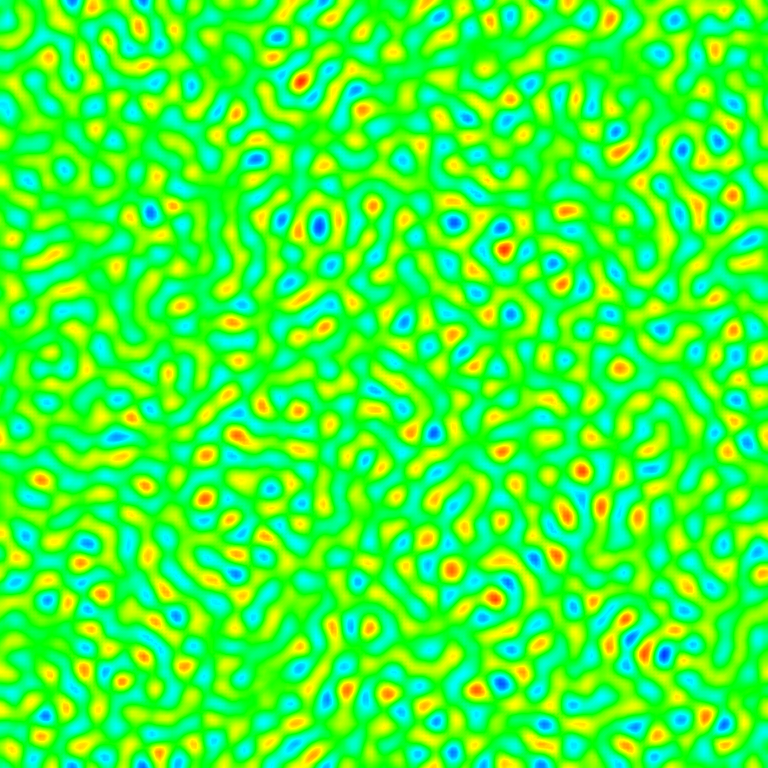
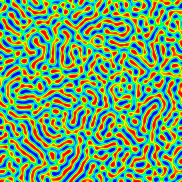
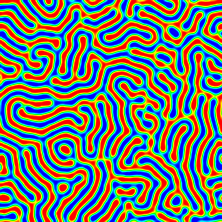
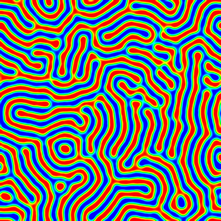
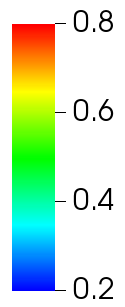
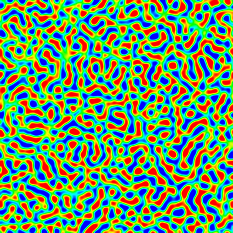
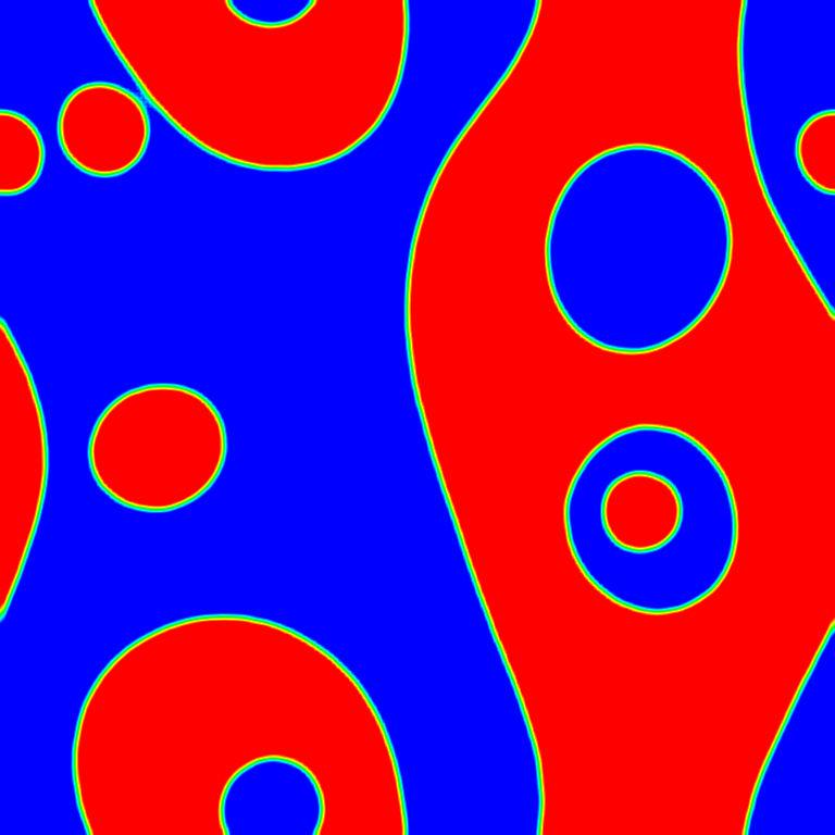
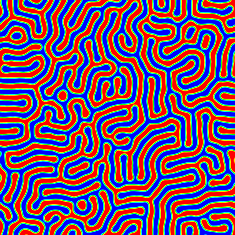
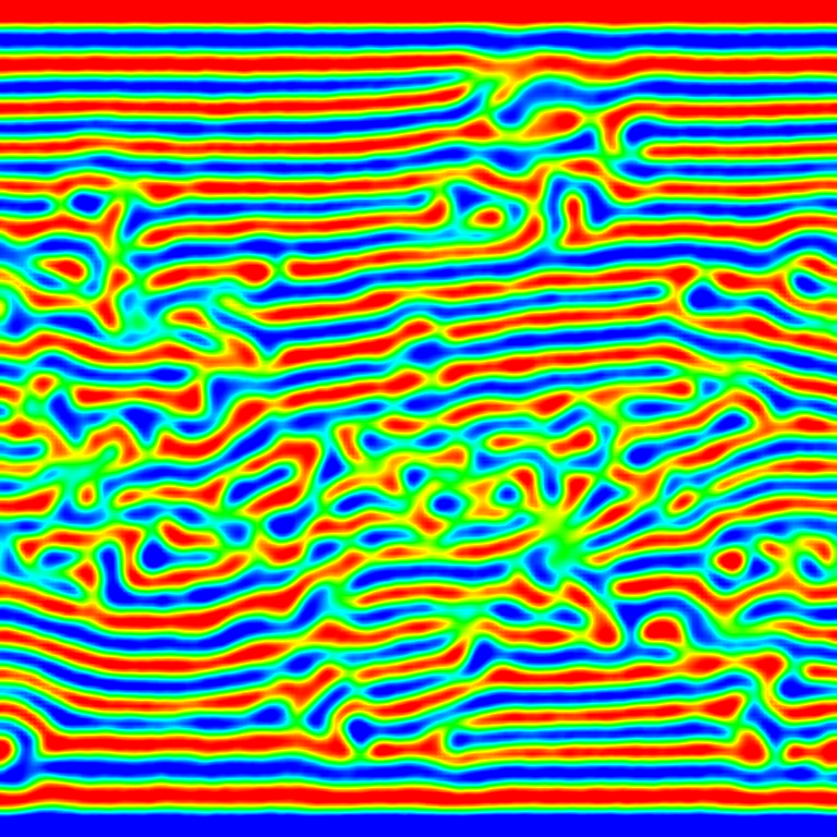
First we consider quasi-two-dimensional systems with periodic boundary conditions. All quasi-two-dimensional simulations in this paper use cells with grid spacings nm and time step . As discussed in Section IV.1, we take for our baseline case; see Table 2 for other parameters. Figure 1 shows the development of patterns that form in a simulation of the RTIL starting from a homogeneous initial condition of . By ns, the morphology nearly reaches the final configuration we show at ns. In fact, at a later time of ns (not pictured), the morphology is nearly identical to the ns frame. This stable feature size reflects the competition between the phase separation and electrostatic forces as discussed in Section IV.1. Also, note that all figures in this paper use the same colobar for cation concentration used in Figure 1 unless otherwise noted.
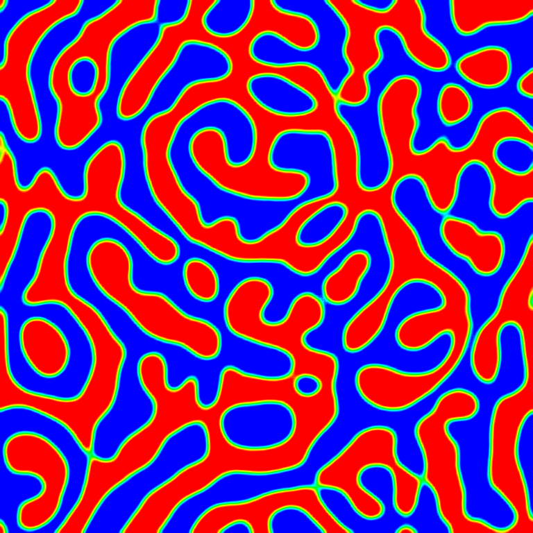
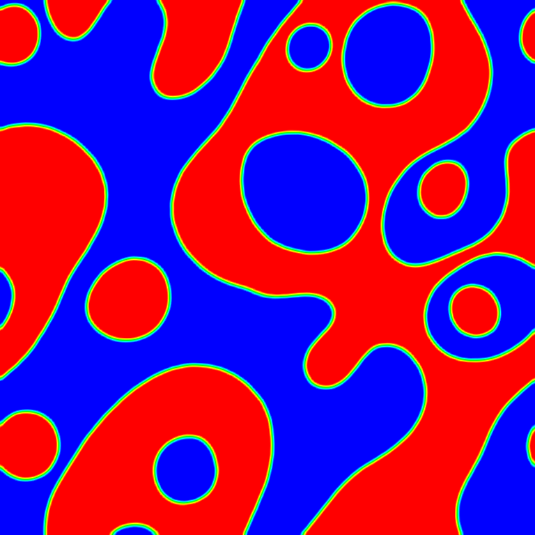
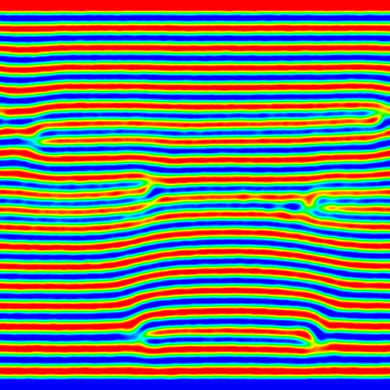
In Figure 2 we show the analogous spinodal decomposition as in Figure 1 but for the case of uncharged species (); here the patterns coarsen quickly and increasingly with time.
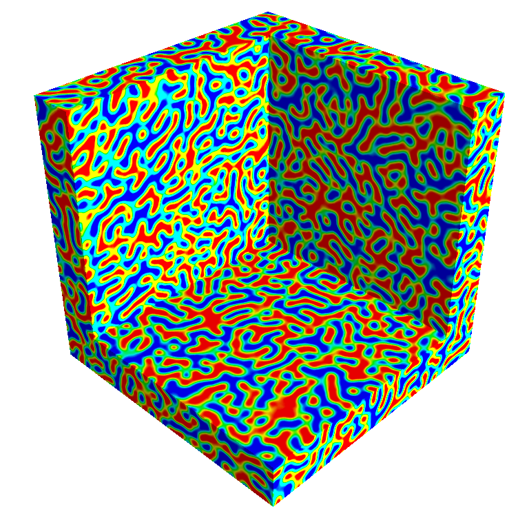
We repeat the simulations, but in three dimensions (see Figure 3) using a cubical domain of cells with the same mesh spacing and time step as before. As in two dimensions, the case with charges evolves to a pattern with fixed feature sizes and then stabilizes whereas the uncharged case coarsens quickly and continues to coarsen over time.


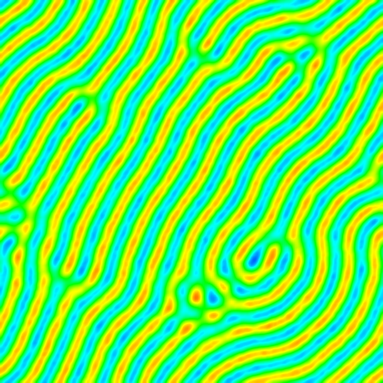
Next we examine how the morphology depends on the interfacial tension parameter, . Figure 4 shows the patterns formed at four additional values of . As increases, the dynamic range of phase separation concentrations decreases. For the largest value shown () the phase separation is almost completely suppressed.


In addition, as increases, the feature size in these patterns becomes larger. To quantify this observation we measured the static structure factor, which is the Fourier transform of the equal time covariance of the concentration,
| (43) |
where the brackets denote an equilibrium average over time and
| (44) |
In each case, we capture statistics for the structure factor by sampling at every time step for 1 ns beginning at ns. Figure 5 shows the structure factor for the and cases. For each value of , the structure factor has a maximum at a radius of . We note that for , we see only a partial ring that reflects the fact that most of the stripes in Figure 4 are oriented in the same direction. The corresponding patterns feature a length scale (i.e., the width of the red or blue structures) that can be found using . We compute by considering to be a probability density function and computing its expected value,
| (45) |
where we only include points in the sum where is above 1% of the peak value, which effectively acts as a white noise filter.
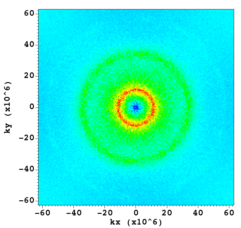
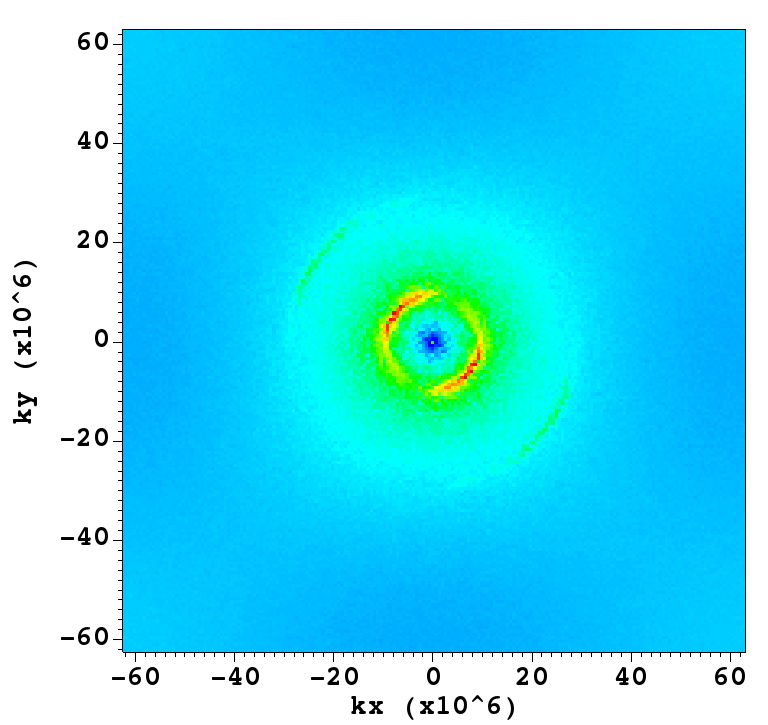
Table 3 lists the values of and for all five values of that we consider (the cases not pictured in Fig. 4 have rings similar to the case). We note that the results for the baseline case with nm are consistent with experimental measurements [50, 51, 48] and molecular dynamics simulations [52, 53] for the RTIL discussed in Section IV.1; for a review see 49. As increases, the associated increases as well, which is consistent with the patterns in Figures 1 and 4. Finally, our three-dimensional simulations using show a spherical structure factor (not pictured) with cm, which matches the two-dimensional case.
| cm | [] | [nm] |
|---|---|---|
| 0.5 | 1.35 | 2.33 |
| 1.0 | 1.14 | 2.76 |
| 1.5 | 1.03 | 3.05 |
| 2.0 | 0.96 | 3.27 |
| 2.5 | 0.92 | 3.41 |
IV.3 Double Layer Capacitance
Consider a charged fluid, either an electrolyte solution or an ionic liquid, confined in a parallel plate capacitor with electrodes at and . The specific differential capacitance of the double layer is defined as where is the surface-charge density and is the overall potential drop between the bulk of electrolyte and the electrode surface. By Gauss’ law, for the electrode wall at ,
| (46) |
With this,
| (47) |
From Gouy-Chapman theory, for a 1:1 electrolyte solution,
| (48) |
and
| (49) |
is the Debye length.
To account for steric effects in ionic liquids Kornyshev [9] formulated a lattice model with a lattice saturation parameter defined as the ratio of the total number of ions to the number of available sites (. This formulation was improved [17] by accounting for the enthalpy of mixing contribution to the free energy, which adds another parameter, , to the model (). For this model the capacitance of the double layer for an ionic liquid with equal size ions is
| (50) |
This reduces to the Gouy-Chapman result for in the limit . Qualitatively the capacitance has the so-called “bell” curve shape for large while for small the capacitance shows a dip near (“camel” shape). The former case is typical of ionic liquids for which the double layer thickness increases with voltage. The latter case corresponds to dilute electrolyte solutions, where for small voltages and the thickness decreases with voltage until steric effects become significant.
We measure the differential capacitance using a series of quasi-two-dimensional simulations. Our simulations use a parallel plate capacitor geometry with no-slip, impermeable, fixed voltage walls in the direction, and periodic in the direction. For each simulation, the voltage at the top and bottom walls are equal in magnitude but opposite in sign; otherwise the parameters used were identical to those used in the periodic simulations in Section IV.2. We performed simulations using 1, 2, 4, 8, 16, 32, 64, and 128 V at the walls for the baseline case of .

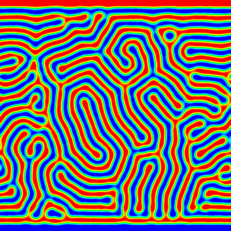
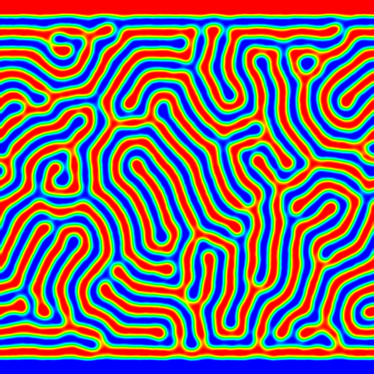
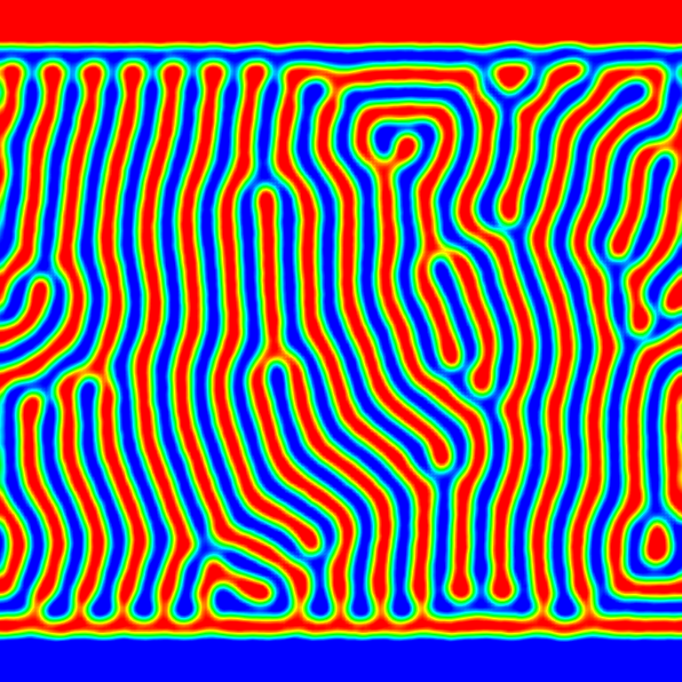
Figure 6 shows the cation concentration after equilibration for several of the cases with varying electrode voltages. The equilibration time depends on the voltage at the walls, with smaller electrode voltages taking longer to fully form the double layer structure, which is why for most of the simulations the voltage was above the electrochemical window of the RTIL [54]. The simulations ran until equilibration, where the patterns had reached a steady configuration (80 ns for runs with V, up to 400 ns for the case). Note that for the largest voltage presented (128V), the morphology features a vertical striped pattern parallel to the strong electric field.
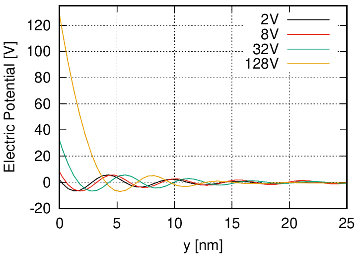
To calculate the capacitance from the simulation data we computed the surface charge density by horizontally averaging and then approximating the normal derivative at the wall using a second-order finite difference approximation using the boundary potential and two interior values. In Figure 7 we show plots of the horizontally-averaged electric potential for the cases depicted in Figure 6. First, we see that the normal derivative of steepens with increasing voltage. The double layer thickness also clearly increases with voltage. We also observe that the amplitude of the patterns a few nanometers away from the wall is similar for all voltages.
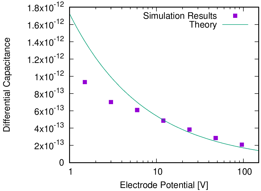
From these simulations we compute the differential capacitance using (47) by estimating the derivative of the surface charge density with respect to voltage using a second-order finite difference approximation. The measured differential capacitance as a function of electrode voltage is shown in Figure 8. The simulation data was curve fit to (50) and the parameter values for the optimal fit were and ; the corresponding curve is also shown in Figure 8. For larger voltages we are able to recover the predicted differential capacitance. For smaller potentials our simulations under-predict the differential capacitance.
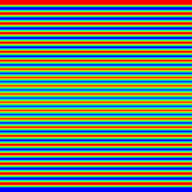
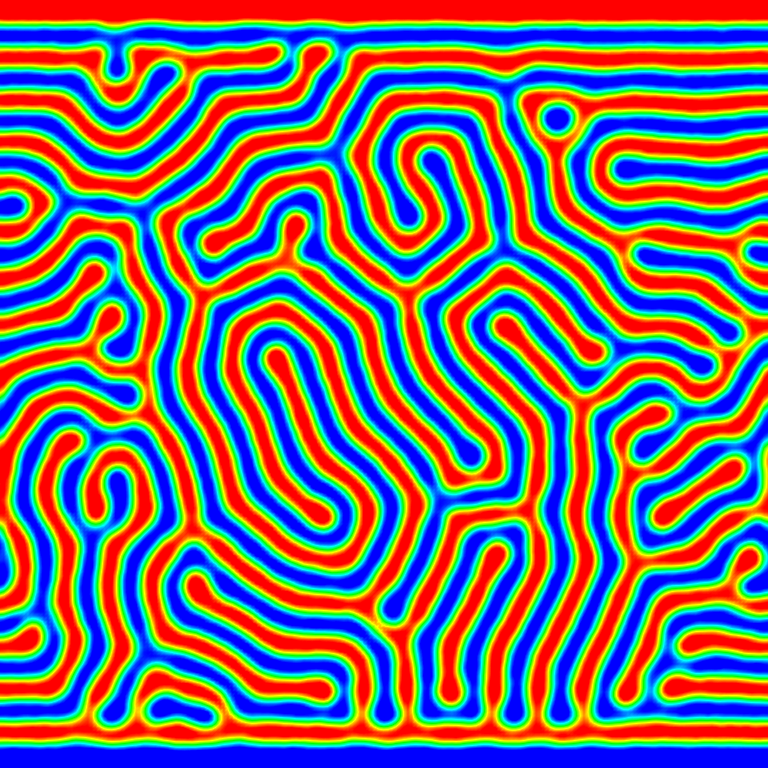
Next we illustrate the effect of the thermal fluctuations in the fluctuating hydrodynamic model of the RTIL. We consider two cases in which the simulations were performed with the stochastic fluxes turned off: a deterministic simulation with a random initial perturbation (first running one time step of the full stochastic algorithm and then turning off the noise terms); and a fully deterministic simulation with a homogeneous initial condition. For the periodic systems considered in Section IV.2 we found little difference between the fully stochastic and the randomly perturbed deterministic simulations. However, if we consider the steady state cation concentration in capacitance simulations with 8 V electrode potentials as shown in Fig. 9, we see that the results for the two deterministic cases are very different from the results for the fully stochastic simulation. The initially perturbed deterministic simulation has a similar morphology, except that horizontal stripes are preferred in the vicinity of the walls. In the fully deterministic simulation, horizontal stripes quickly form across the domain. These stripes do not have a consistent structure size; they are thinner at the center of the domain and thickest near the walls.
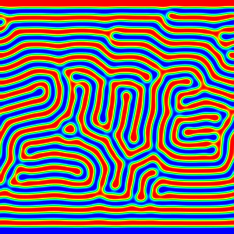
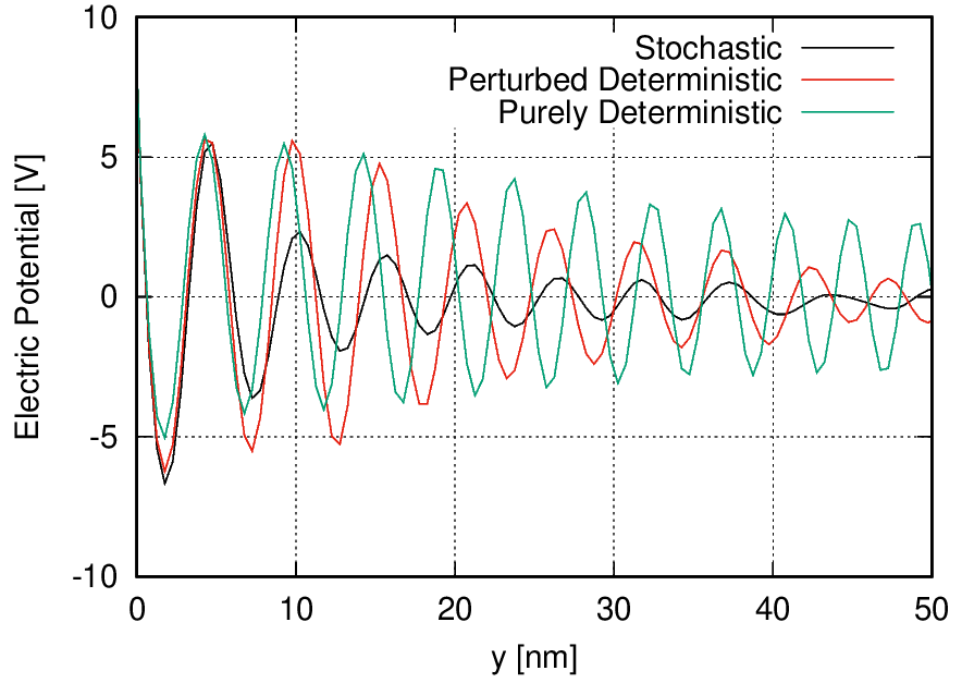
In Figure 10 we show horizontally-averaged profiles of the electric potential for these same three cases which further confirm these observations. The perturbed deterministic simulation shows a slower decrease in the potential away from the wall due to the horizontal striping (constructive interference in the horizontal averaging), and in the purely deterministic case the wavelength of the oscillations is clearly smaller.
IV.4 Electroosmotic shear flow
Electroosmotic flow occurs when an external electric field is applied parallel to the electric double layer near an electrode wall. Since the double layer is not electroneutral the ions near the wall experience a Lorentz force, which results in a body force on the fluid. For channel walls of equal potential (or surface charge density) electroosmosis results in a plug flow for wide channels () and Poiseuille-type flow in narrow channels. Here we consider electrode walls of opposite potential, as in the parallel plate capacitor geometry described in the previous section, which results in electroosmotic shear flow. Specifically we consider electrodes with potentials of V and impose an external electric field in the direction corresponding to a 500V potential drop across the domain. The resulting shear rate from the electroosmotic flow is about .

The temporal evolution of the resulting sheared system is shown in Figure 11. For the strong imposed electric field considered in this example, the shearing first destroys the serpentine patterns and then structure is restored, developing a striated pattern parallel to the imposed electric field with a few long-lived defects. Molecular dynamics studies also indicate that nanostructures in RTILs persist in the presence of a strong shear.[55, 56]
V Conclusions
The computational model presented here is the first step towards a mesoscale simulation capability for room temperature ionic liquids that includes both hydrodynamics and thermal fluctuations. The fluctuating hydrodynamics formulation for RTILs is a useful intermediary, mesoscale theory bridging microscopic models, such as molecular dynamics, and macroscopic models.The low Mach number formulation avoids the severe time step restriction associated with previous compressible formulations. We have demonstrated in both two and three dimensions that resulting methodology reproduces the microscopic structuring observed in RTILs. We also used the methodology to show that the differential capacitance decreases with applied voltage which is a characteristic of ionic liquids. The morphology patterns observed in this capacitance geometry were significantly different depending on whether the simulations included or excluded thermal fluctuations. Finally, the shear electroosmosis example shows that the methodology can be used to model electrokinetic flows.
The present model can be enhanced and extended in several important directions in the future. In this paper we considered a two-component ionic fluid with symmetric ions; however, the RTIL model can be generalized to arbitrary multi-component mixtures. (See 32 for a more general FHD model of multicomponent electrolyte solutions.) This will allow us to consider RTILs composed of dissimilar ions as well as investigate the effect of a polar solvent on the structural, thermodynamic, and electrical properties.
As is commonly assumed in RTIL modeling we assumed the permittivity to be a constant. A more realistic version of the model makes the permittivity a function of concentration, which is important for the study of RTIL mixtures. The implementation requires modifying the calculation of the Poisson equation and the Maxwell stress tensor; a greater challenge is determining an accurate functional form of . A related extension is to include dielectric relaxation [57] by treating the local permittivity (or equivalently, the local polarization density) as a stochastic quantity whose dynamics are given by a Langevin equation.
The increased time step associated with the low Mach number fluctuating hydrodynamics model makes it possible to investigate long time dynamics and three dimensional effects. Many ionic liquids tend to have glassy behaviors [58, 59] that make the equilibration of molecular dynamics simulations particularly challenging. Our fluctuating hydrodynamics model permits numerical explorations of RTIL regimes with slow dynamics. The capability to perform three dimensional simulations is particularly important for future investigations of the structure and dynamics of the double layer. The transitions between lateral arrangements of counter and co-ions at electrified interfaces greatly affects the capacitance and dynamics of the double layers, and this is related to the three-dimensional nature of the double layer in ionic liquids [60]. As part of this type of investigation, more physically realistic boundary conditions that can capture wetting effects at electrode-RTIL interfaces will need to be introduced.
Generalization of the methodology to more complex boundary conditions and geometries would allow us to explore capacitance enhancement in nanopores [61], which are important in the development of supercapacitors based on nanostructured electrodes. The treatment of electrochemical effects at electrode boundaries would be a topic for future work.
Finally, the FHD methodology presented here lays the foundation for hybrid, or “heterogeneous" methods [62, 63, 64] that couple a continuum hydrodynamic description to a more detailed microscopic model, e.g., molecular dynamics. For these types of “Adaptive Algorithm” hybrids, the continuum model needs to include thermal fluctuations in order to correctly capture the behavior in the region being modeled with the microscopic model [65]. This type of hybrid model would enable simulations to use a microscopic representation locally where molecular-level accuracy is desired, such as near electrode surfaces, while using a less expensive continuum-based model in the remainder of the domain.
Acknowledgements
This work was supported by the U.S. Department of Energy, Office of Science, Office of Advanced Scientific Computing Research, Applied Mathematics Program under contract No. DE-AC02-05CH11231. This research used resources of the National Energy Research Scientific Computing Center, a DOE Office of Science User Facility supported by the Office of Science of the U.S. Department of Energy under Contract No. DE-AC02-05CH11231.
Appendix A Derivation of Inviscid Hydrodynamic Equation
Here we derive the inviscid form of the momentum equation (4) using the calculus of variations. It will be useful below to introduce the notation
| (51) |
for the advective derivative of scalar with respect to the velocity field . For the case when is a vector of functions, equation (51) is understood component-wise, so that in Einstein notation
| (52) |
Starting from the action
| (53) |
which is simply the space-time integral of the kinetic energy of the fluid minus the time integral of the free energy functional (see eqn. (1)), we add the constraints that the flow is divergence free and that the concentration is advected by the flow. The action then becomes
| (54) |
where and are the Lagrange multipliers. These extra constraints are necessary for nontrivial dynamics for the velocity field; enforcing that the action is stationary with respect to variations in results in
| (55) |
after integrating by parts and assuming the space of trial functions is such that the boundary terms vanish. This is the well-known Clebsch representation [66, 67]. Variations with respect to and result in the Poisson equation of electrostatics and the divergence-free constraint
| (56) | ||||
| (57) |
Variations with respect to and using (57) result in the constraint
| (58) |
Consider now the advective derivative of the Clebsch representation (55), and note that is a linear operator that obeys the standard product rule of differential calculus , as well as the commutation relation
| (59) |
where the second term is a matrix-vector product and is defined as . Hence
| (60) | |||||
| (61) | |||||
| (62) | |||||
| (63) | |||||
The term will be the source of the Lorentz force density (15) and the divergence of the interfacial reversible stress (16).
It remains to consider variations of the action with respect to the concentration . Grouping together the contributions to the specific free energy modeling the enthalpy and entropy of mixing into a single term
| (64) |
eqn. (2) becomes
| (65) |
Variations with respect to then result in
| (66) | ||||
| (67) |
After manipulating the three terms on the right hand side of (67), we will insert them into (63). The third term can be written as
| (68) | ||||
| (69) | ||||
| (70) |
using the definition of the Maxwell stress tensor (15). The second term can be written by combining the two product rule identities:
| (71) |
and
| (72) | ||||
| (73) |
so that
| (74) | ||||
| (75) | ||||
| (76) |
by definition of the interfacial reversible stress tensor (16). Lastly, the first term on the right hand side of equation (67) can be re-written using the Gibbs-Duhem relation of thermodynamics [36], which says for our isothermal, two-component mixture
| (77) |
where is the thermodynamic pressure and . Since , , and ,
| (78) |
and hence the Gibbs-Duhem relation reduces to
| (79) | ||||
| (80) |
Inserting the relations (80), (76), and (70) into the term in (63) then results in
| (81) | ||||
| (82) |
and after identifying
| (83) |
as a perturbational pressure, we arrive at the inviscid form of the momentum equation in (1)
| (84) |
as desired.
References
- [1] D. Silvester and R. Compton. Electrochemistry in room temperature ionic liquids: A review and some possible applications. Zeitschrift für Physikalische Chemie, 220:1247–1274, 2009.
- [2] James Wishart. Energy applications of ionic liquids. Royal Society of Chemistry, 2:956–961, 2009.
- [3] Hiroyuki Tokuda, Seiji Tsuzuki, Md. Abu Bin Hasan Susan, Kikuko Hayamizu, and Masayoshi Watanabe. How ionic are room-temperature ionic liquids? an indicator of the physicochemical properties. The Journal of Physical Chemistry B, 110(39):19593–19600, 2006.
- [4] A. Brandt, S. Pohlmann, A. Varzi, A. Balducci, and S. Passerini. Ionic liquids in supercapacitors. MRS Bulletin, 38(7):554––559, 2013.
- [5] Andrzej Lewandowski and Agnieszka Świderska Mocek. Ionic liquids as electrolytes for li-ion batteries—an overview of electrochemical studies. Journal of Power Sources, 194(2):601 – 609, 2009.
- [6] Qinghua Li, Qunwei Tang, Benlin He, and Peizhi Yang. Full-ionic liquid gel electrolytes: Enhanced photovoltaic performances in dye-sensitized solar cells. Journal of Power Sources, 264:83 – 91, 2014.
- [7] Feng Zhou, Yongmin Liang, and Weimin Liu. Ionic liquid lubricants: designed chemistry for engineering applications. Royal Society of Chemistry, 38:2590–2599, 2009.
- [8] Anthony E. Somers, Patrick C. Howlett, Douglas R. MacFarlane, and Maria Forsyth. A review of ionic liquid lubricants. Lubricants, 1(1):3–21, 2013.
- [9] Alexei A. Kornyshev. Double-layer in ionic liquids: paradigm change? The Journal of Physical Chemistry B, 111(20):5545–5557, 2007. PMID: 17469864.
- [10] Martin Z Bazant, Brian D Storey, and Alexei A Kornyshev. Double layer in ionic liquids: Overscreening versus crowding. Physical Review Letters, 106(4):046102, 2011.
- [11] Céline Merlet, David T. Limmer, Mathieu Salanne, René van Roij, Paul A. Madden, David Chandler, and Benjamin Rotenberg. The electric double layer has a life of its own. The Journal of Physical Chemistry C, 118(32):18291–18298, 2014.
- [12] Edward J Maginn. Atomistic simulation of the thermodynamic and transport properties of ionic liquids. Accounts of chemical research, 40(11):1200–1207, 2007.
- [13] Nav Nidhi Rajput, Joshua Monk, and Francisco R Hung. Structure and dynamics of an ionic liquid confined inside a charged slit graphitic nanopore. The Journal of Physical Chemistry C, 116(27):14504–14513, 2012.
- [14] Ge-Bo Pan and Werner Freyland. 2d phase transition of pf6 adlayers at the electrified ionic liquid/au(111) interface. Chemical Physics Letters, 427(1):96 – 100, 2006.
- [15] Yu-Zhuan Su, Yong-Chun Fu, Jia-Wei Yan, Zhao-Bin Chen, and Bing-Wei Mao. Double layer of au(100)/ionic liquid interface and its stability in imidazolium-based ionic liquids. Angewandte Chemie International Edition, 48(28):5148–5151, 2009.
- [16] Rui Wen, Björn Rahn, and Olaf M. Magnussen. Potential-dependent adlayer structure and dynamics at the ionic liquid/au(111) interface: A molecular-scale in situ video-stm study. Angewandte Chemie International Edition, 54(20):6062–6066, 2015.
- [17] Zachary A.H. Goodwin, Guang Feng, and Alexei A. Kornyshev. Mean-field theory of electrical double layer in ionic liquids with account of short-range correlations. Electrochimica Acta, 225:190 – 197, 2017.
- [18] Monchai Jitvisate and James RT Seddon. Direct measurement of the differential capacitance of solvent-free and dilute ionic liquids. The journal of physical chemistry letters, 9(1):126–131, 2018.
- [19] Martin Z. Bazant, Brian D. Storey, and Alexei A. Kornyshev. Double layer in ionic liquids: Overscreening versus crowding. Phys. Rev. Lett., 106:046102, Jan 2011.
- [20] David T. Limmer. Interfacial ordering and accompanying divergent capacitance at ionic liquid-metal interfaces. Phys. Rev. Lett., 115:256102, Dec 2015.
- [21] Nir Gavish and Arik Yochelis. Theory of phase separation and polarization for pure ionic liquids. The Journal of Physical Chemistry Letters, 7(7):1121–1126, 2016. PMID: 26954098.
- [22] Takao Ohta and Kyozi Kawasaki. Equilibrium morphology of block copolymer melts. Macromolecules, 19(10):2621–2632, 1986.
- [23] Kyozi Kawasaki, Takao Ohta, and Mitsuharu Kohrogui. Equilibrium morphology of block copolymer melts. 2. Macromolecules, 21:2972–2980, 1988.
- [24] David J Bozym, Betül Uralcan, David T Limmer, Michael A Pope, Nicholas J Szamreta, Pablo G Debenedetti, and Ilhan A Aksay. Anomalous capacitance maximum of the glassy carbon–ionic liquid interface through dilution with organic solvents. The journal of physical chemistry letters, 6(13):2644–2648, 2015.
- [25] De-en Jiang, Dong Meng, and Jianzhong Wu. Density functional theory for differential capacitance of planar electric double layers in ionic liquids. Chemical Physics Letters, 504(4-6):153–158, 2011.
- [26] Sergey A Katsyuba, Elena E Zvereva, Ana Vidiš, and Paul J Dyson. Application of density functional theory and vibrational spectroscopy toward the rational design of ionic liquids. The Journal of Physical Chemistry A, 111(2):352–370, 2007.
- [27] Konstantinos Lazaridis, Logan Wickham, and Nikolaos Voulgarakis. Fluctuating hydrodynamics for ionic liquids. Physics Letters A, 381(16):1431 – 1438, 2017.
- [28] J. Lowengrub and L. Truskinovsky. Quasi–incompressible Cahn–Hilliard fluids and topological transitions. Proceedings of the Royal Society, A, 454:2617–2654, 1998.
- [29] Aleksandar Donev, Andy Nonaka, Yifei Sun, Thomas Fai, Alejandro Garcia, and John Bell. Low mach number fluctuating hydrodynamics of diffusively mixing fluids. Communications in Applied Mathematics and Computational Science, 9(1):47–105, 2014.
- [30] Andrew Nonaka, Yifei Sun, John Bell, and Aleksandar Donev. Low mach number fluctuating hydrodynamics of binary liquid mixtures. Communications in Applied Mathematics and Computational Science, 10(2):163–204, 2015.
- [31] Aleksandar Donev, Andy Nonaka, Amit Kumar Bhattacharjee, Alejandro L Garcia, and John B Bell. Low mach number fluctuating hydrodynamics of multispecies liquid mixtures. Physics of Fluids, 27(3):037103, 2015.
- [32] Jean-Philippe Péraud, Andy Nonaka, Anuj Chaudhri, John B. Bell, Aleksandar Donev, and Alejandro L. Garcia. Low mach number fluctuating hydrodynamics for electrolytes. Phys. Rev. Fluids, 1:074103, Nov 2016.
- [33] Aleksandar Donev, Andrew J Nonaka, Changho Kim, Alejandro L Garcia, and John B Bell. Fluctuating hydrodynamics of electrolytes at electroneutral scales. Physical Review Fluids, 4(4):043701, 2019.
- [34] Sergiu Klainerman and Andrew Majda. Compressible and incompressible fluids. Communications on Pure and Applied Mathematics, 35(5):629–651, 1982.
- [35] Andrew Majda and James Sethian. The derivation and numerical solution of the equations for zero mach number combustion. Combustion Science and Technology, 42(3-4):185–205, 1985.
- [36] S. R. DeGroot and P. Mazur. Non-Equilibrium Thermodynamics. North-Holland Publishing Company, Amsterdam, 1963.
- [37] L. D. Landau and E. M. Lifshitz. Fluid Mechanics, Course of Theoretical Physics, Vol. 6. Pergamon Press, 1959.
- [38] J. M. Ortiz de Zarate and J. V. Sengers. Hydrodynamic Fluctuations in Fluids and Fluid Mixtures. Elsevier Science, 2007.
- [39] R Kubo. The fluctuation-dissipation theorem. Reports on Progress in Physics, 29(1):255–284, 1966.
- [40] LD Landau, EM Lifshitz, and LP Pitaevskii. Electrodynamics of continuous media, 1984. Moscow Science, 1992.
- [41] Barry Z Shang, Nikolaos K Voulgarakis, and Jhih-Wei Chu. Fluctuating hydrodynamics for multiscale simulation of inhomogeneous fluids: Mapping all-atom molecular dynamics to capillary waves. The Journal of chemical physics, 135(4):044111, 2011.
- [42] A. Donev, E. Vanden-Eijnden, A. L. Garcia, and J. B. Bell. On the accuracy of finite-volume schemes for fluctuating hydrodynamics. Comm. Appl. Math and Comp. Sci., 5(2):149, 2010.
- [43] F. Balboa Usabiaga, J.B. Bell, R. Delgado-Buscalioni, A. Donev, T.G. Fai, B.E. Griffith, and C. Peskin. Staggered schemes for fluctuating hydrodynamics. Multiscale Modeling & Simulation, 10(4):1369–1408, 2012.
- [44] Mingchao Cai, Andy Nonaka, John B. Bell, Boyce E. Griffith, and Aleksandar Donev. Efficient variable-coefficient finite-volume stokes solvers. Communications in Computational Physics, 16(5):1263–1297, 2014.
- [45] Martin Gouverneur, Jakob Kopp, Leo van Wüllen, and Monika Schönhoff. Direct determination of ionic transference numbers in ionic liquids by electrophoretic nmr. Phys. Chem. Chem. Phys., 17:30680–30686, 2015.
- [46] Hiroyuki Tokuda, Seiji Tsuzuki, Md. Abu Bin Hasan Susan, Kikuko Hayamizu, and Masayoshi Watanabe. How ionic are room-temperature ionic liquids? an indicator of the physicochemical properties. The Journal of Physical Chemistry B, 110(39):19593–19600, 2006.
- [47] Hongbo Zhao, Brian D. Storey, Richard D. Braatz, and Martin Z. Bazant. Learning the physics of pattern formation from images. Phys. Rev. Lett., 124:060201, Feb 2020.
- [48] Christopher Hardacre, John D. Holbrey, Claire L. Mullan, Tristan G. A. Youngs, and Daniel T. Bowron. Small angle neutron scattering from 1-alkyl-3-methylimidazolium hexafluorophosphate ionic liquids ([cnmim][pf6], n=4, 6, and 8). The Journal of Chemical Physics, 133(7):074510, 2010.
- [49] Robert Hayes, Gregory G. Warr, and Rob Atkin. Structure and nanostructure in ionic liquids. Chemical Reviews, 115:6357–6426, 2015.
- [50] Alessandro Triolo, Andrea Mandanici, Olga Russina, Virginia Rodriguez-Mora, Maria Cutroni, Christopher Hardacre, Mark Nieuwenhuyzen, Hans-Jurgen Bleif, Lukas Keller, and Miguel Angel Ramos. Thermodynamics, structure, and dynamics in room temperature ionic liquids: the case of 1-butyl-3-methyl imidazolium hexafluorophosphate ([bmim][pf6]). The Journal of Physical Chemistry B, 110(42):21357–21364, 2006.
- [51] Alessandro Triolo, Olga Russina, Hans-Jurgen Bleif, and Emanuela Di Cola. Nanoscale segregation in room temperature ionic liquids. The Journal of Physical Chemistry B, 111(18):4641–4644, 2007.
- [52] Timothy I. Morrow and Edward J. Maginn. Molecular dynamics study of the ionic liquid 1-n-butyl-3-methylimidazolium hexafluorophosphate. The Journal of Physical Chemistry B, 106(49):12807–12813, 2002.
- [53] Zhiping Liu, Shiping Huang, and Wenchuan Wang. A refined force field for molecular simulation of imidazolium-based ionic liquids. The Journal of Physical Chemistry B, 108(34):12978–12989, 2004.
- [54] Marisa C. Buzzeo, Russell G. Evans, and Richard G. Compton. Non-haloaluminate room-temperature ionic liquids in electrochemistry—a review. ChemPhysChem, 5(8):1106–1120, 2004.
- [55] S G Raju and S Balasubramanian. Intermolecular correlations in an ionic liquid under shear. Journal of Physics: Condensed Matter, 21(3):035105, dec 2008.
- [56] Simon N. Butler and Florian Müller-Plathe. Nanostructures of ionic liquids do not break up under shear: A molecular dynamics study. Journal of Molecular Liquids, 192:114 – 117, 2014. Fundamental Aspects of Ionic Liquid Science.
- [57] Alexander Stoppa, Richard Buchner, and Glenn Hefter. How ideal are binary mixtures of room-temperature ionic liquids? Journal of Molecular Liquids, 153(1):46 – 51, 2010.
- [58] Joshua R Sangoro and Friedrich Kremer. Charge transport and glassy dynamics in ionic liquids. Accounts of chemical research, 45(4):525–532, 2012.
- [59] Falk Frenzel, Pia Borchert, Arthur Markus Anton, Veronika Strehmel, and Friedrich Kremer. Charge transport and glassy dynamics in polymeric ionic liquids as reflected by their inter-and intramolecular interactions. Soft matter, 15(7):1605–1618, 2019.
- [60] Alexei A. Kornyshev and Rui Qiao. Three-dimensional double layers. The Journal of Physical Chemistry C, 118(32):18285–18290, 2014.
- [61] Clarisse Péan, Céline Merlet, Benjamin Rotenberg, Paul Anthony Madden, Pierre-Louis Taberna, Barbara Daffos, Mathieu Salanne, and Patrice Simon. On the dynamics of charging in nanoporous carbon-based supercapacitors. ACS nano, 8(2):1576–1583, 2014.
- [62] Alejandro L Garcia, John B Bell, William Y Crutchfield, and Berni J Alder. Adaptive mesh and algorithm refinement using direct simulation monte carlo. Journal of Computational Physics, 154(1):134 – 155, 1999.
- [63] Assyr Abdulle, E Weinan, Björn Engquist, and Eric Vanden-Eijnden. The heterogeneous multiscale method. Acta Numerica, 21:1–87, 2012.
- [64] Luigi Delle Site, Matej Praprotnik, John B. Bell, and Rupert Klein. Particle–continuum coupling and its scaling regimes: Theory and applications. Advanced Theory and Simulations, n/a(n/a):1900232, 2020.
- [65] A. Donev, J. B. Bell, A. L. Garcia, and B. J. Alder. A hybrid particle-continuum method for hydrodynamics of complex fluids. SIAM J. Multiscale Modeling and Simulation, 8:871–911, 2010.
- [66] A. Clebsch. Ueber die integration der hydrodynamischen gleichungen. Journal für die reine und angewandte Mathematik, 1859(56):1 – 10, 1859.
- [67] Rick Salmon. Hamiltonian fluid mechanics. Annual review of fluid mechanics, 20(1):225–256, 1988.