Causal inference under outcome-based sampling with monotonicity assumptions

Abstract

We study causal inference under case-control and case-population sampling. Specifically, we focus on the binary-outcome and binary-treatment case, where the parameters of interest are causal relative and attributable risks defined via the potential outcome framework. It is shown that strong ignorability is not always as powerful as it is under random sampling and that certain monotonicity assumptions yield comparable results in terms of sharp identified intervals. Specifically, the usual odds ratio is shown to be a sharp identified upper bound on causal relative risk under the monotone treatment response and monotone treatment selection assumptions. We offer algorithms for inference on the causal parameters that are aggregated over the true population distribution of the covariates. We show the usefulness of our approach by studying three empirical examples: the benefit of attending private school for entering a prestigious university in Pakistan; the relationship between staying in school and getting involved with drug-trafficking gangs in Brazil; and the link between physicians’ hours and size of the group practice in the United States.

Abstract

In appendices A, B and C, we discuss aggregation of $\theta_{\mathrm{RR}}(\cdot)$ without taking the logarithm, efficient estimation of $\beta(y)$ for $y=0,1$, and the results of a small Monte Carlo experiment, respectively. Appendix D gives details on inference issues omitted in section 5, and appendix E presents proofs.

Keywords: Relative risk; attributable risk; odds ratio; partial identification

1 Introduction

Random sampling is convenient for causal inference, but it may be too costly in practice for various reasons. For instance, rare events are likely to be severely under-represented in a random sample of a finite size: e.g., cancer (Breslow & Day 1980), infant death (Currie & Neidell 2005), consumer bankruptcy (Domowitz & Sartain 1999), entering a highly prestigious university (Delavande & Zafar 2019), and drug trafficking (Carvalho & Soares 2016). The objective of this paper is to study causal inference in outcome-based sampling scenarios such as case-control or case-population studies.

We focus on observational data, as opposed to experimental ones, with a binary outcome and a binary treatment. Holland & Rubin (1988) adopt the potential outcome framework to show that the assumption of strong ignorability can be used to identify the counterfactual odds ratio in case-control studies. They then argue that the counterfactual odds ratio approximates the ratio of two potential-outcome probabilities (i.e., causal relative risk) under the rare-disease assumption, which says that the probability of outcome occurrence (e.g., having “a certain disease”) is close to zero. Their work is our starting point, and we make additional contributions in several ways.

First, we focus on two direct causal parameters (i.e., a ratio or a difference of two potential-outcome probabilities) that are more straightforward to interpret than counterfactual odds ratios: our parameters of interest are the causal relative and attributable risks given a specific value of covariates. Second, we do not appeal to the rare-disease assumption, and we take the perspective of partial identification (see, e.g., Manski 1995, 2003, 2007, Tamer 2010, Molinari 2020, among others). Third, we consider a set of monotonicity assumptions, and we compare their identification power with that of strong ignorability. Strong ignorability is a popular setup for causal inference, but its identification power in outcome-based sampling turns out to be somewhat limited. Specifically, in case-control or case-population studies, strong ignorability is generally not sufficient to point identify the causal relative and attributable risks. We can obtain bounds on them, but they are not much better than those we can obtain in a less restrictive setup using monotonicity. Specifically, we will consider monotone treatment response (Manski 1997, MTR hereafter) and monotone treatment selection (Manski & Pepper 2000, MTS hereafter).

Our work builds upon Manski (2007, Ch 6), who conducts a partial identification analysis for both relative and attributable risks under outcome-based sampling without focusing on causal parameters. The MTR and MTS assumptions as well as other related notions of monotonicity have been extensively used in the literature. For example, see Vytlacil & Yildiz (2007), Bhattacharya et al. (2008, 2012), Pearl (2009), VanderWeele & Robins (2009), Kreider et al. (2012), Jiang et al. (2014), Okumura & Usui (2014), Choi (2017), Kim et al. (2018), and Machado et al. (2019) among others.

We now discuss the relation of our work with the existing literature on causal inference under outcome-based sampling. Månsson et al. (2007) point out that the propensity score method has only limited ability to control for confounding factors in case-control studies. Our method does not rely on the propensity score. Rose (2011) and Van der Laan & Rose (2011) use an assumption that the true case probability is known by a prior study. We focus on the instance of unknown case probability. Didelez & Evans (2018) provide an extensive survey on causal inference in case-control studies, but no discussion on partial identification approaches can be found there. Therefore, possibilities based on partial identification appear to be rather underexplored. Kuroki et al. (2010) and Gabriel et al. (2022) are notable exceptions. Gabriel et al. (2022) obtain bounds on the causal attributable risk in a variety of scenarios including outcome-dependent sampling with an instrumental variable. But they do not leverage any monotonicity assumption, while we do not consider instrumental variables but we use monotonicity restrictions. Kuroki et al. (2010) is more similar to our work in that they obtain bounds on both the causal relative and attributable risks by using the MTR assumption. Our contributions relative to Kuroki et al. (2010) can be highlighted as follows: (1) we exploit not only the MTR but also the MTS assumption, and therefore the bounds are different; (2) we consider case-control sampling as well as case-population sampling; (3) we compare the identification power of the popular assumption of strong ignorability with that of the MTR and MTS assumptions; (4) we consider how to aggregate the causal parameters over the distribution of the covariates; and (5) we provide algorithms for causal inference.

The remaining part of the paper is organized as follows. In section 2 we formally present the setup including the causal parameters of interest and the sampling schemes. Sections 3 and 4 focus on the causal relative risk and attributable risk to address identification and aggregation. Section 5 covers how to carry out causal inference. Section 6 presents three empirical applications. Specifically, by using datasets collected in previous studies, we address new research questions that are not examined in the original papers. All the proofs, discussions on semiparametric efficiency and computational algorithms are in Online Appendix. An accompanying R package is available on the Comprehensive R Archive Network (CRAN) at https://CRAN.R-project.org/package=ciccr, and the replication files are available at https://github.com/sokbae/replication-JunLee-JBES.

2 Preliminaries

2.1 Causal parameters

Let $(Y^{*},T^{*},X^{*})$ be a random vector of a binary outcome, a binary treatment, and covariates of a representative individual. Since we are interested in outcome-based sampling, we assume that a random sample of $(Y^{*},T^{*},X^{*})$ is not available. Instead, we have a sample of $(Y,T,X)$, where the distribution of $(T,X)$ given $Y$ is related with that of $(T^{*},X^{*})$ given $Y^{*}$. The exact sampling schemes and related assumptions will be discussed in detail later, and in this subsection, we only focus on the parameters of interest.

For the sake of causal inference, we use the usual potential outcome notation. So, $Y^{*}(t)$ will be the potential outcome for $T^{*}=t$, and $Y^{*}$ can be written as $Y^{*}=Y^{*}(1)T^{*}+Y^{*}(0)(1-T^{*})$. Therefore, our notation extends Chen (2001) and Xie et al. (2020) by adding an extra layer of potential outcomes. The causal effect of the treatment can be measured by either (conditional) relative risk or attributable risk: each of them is defined as follows:

$$\theta_{\mathrm{RR}}(x) :=\frac{\mathbb{P}\{Y^{*}(1)=1\mid X^{*}=x\}}{\mathbb{P}\{Y^{*}(0)=1\mid X^{*}=x\}},$$ (1)

$$\theta_{\mathrm{AR}}(x) :=\mathbb{P}\{Y^{*}(1)=1\mid X^{*}=x\}-\mathbb{P}\{Y^{*}(0)=1\mid X^{*}=x\},$$ (2)

provided that the denominator of $\theta_{\mathrm{RR}}(x)$ is strictly positive. Therefore, $\theta_{\mathrm{AR}}(x)$ is the usual conditional average treatment effect, whereas $\theta_{\mathrm{RR}}(x)$ is a causal version of the relative risk parameter.

Relative risk defined by a ratio of “success” probabilities has been popular in epidemiology and biostatistics, particularly when the “success” is a rare event: if the treatment changes the success probability from $0.01$ to $0.02$, then it is a 100% increase, though the difference of $0.01$ may suggest an impression that the change was unimportant. Further, it turns out that $\theta_{\mathrm{RR}}(x)$ is closely related with the odds ratio (in terms of the observed variables), which has been widely used as a measure of association in case-control studies.

2.2 Bernoulli sampling

As we mentioned earlier, we assume that a random sample of $(Y^{*},T^{*},X^{*})$ is unavailable. Instead the researcher has access to a random sample of $(Y,T,X)$, where the distribution of $(Y,T,X)$ is related with that of $(Y^{*},T^{*},X^{*})$ by Bernoulli sampling (e.g. Breslow et al. 2000) that we describe below.

In Bernoulli sampling, the researcher first draws a Beroulli variable $Y$ from a pre-specified marginal distribution, after which she randomly draws $(T,X)$ from some $\mathcal{P}_{y}$ if and only if $Y=y$; so, $Y$ is an artificial device to decide which subpopulation we will draw $(T,X)$ from. If $\mathcal{P}_{y}$ is the distribution of $(T^{*},X^{*})$ conditional on $Y^{*}=y$, then this is nothing but case-control sampling. Since $h_{0}=\mathbb{P}(Y=1)\in(0,1)$ is part of the sampling scheme, we will assume that it is known; if not, it can be easily estimated without compromising inferential validity. See online appendices B.1 and B.2 for more details. Before we proceed, we make a common support assumption for simplification.

Assumption A (Common Support).

The support of $X^{*}$ and that of $X$ given $Y=y$ for $y=0,1$ coincide; the common support will be denoted by $\mathcal{X}$.

Below we discuss two leading cases of Bernoulli sampling that we focus on throughout the paper.

Design 1 (Case-Control Sampling).

For $y\in\{0,1\}$, $\mathcal{P}_{y}$ is the distribution of $(T^{*},X^{*})$ given $Y^{*}=y$.

Design 2 (Case-Population Sampling).

$\mathcal{P}_{1}$ is the conditional distribution of $(T^{*},X^{*})$ given $Y^{*}=1$, whereas $\mathcal{P}_{0}$ represents the distribution of $(T^{*},X^{*})$ of the entire population.

Design 1 is arguably the most popular form of case-control studies (e.g., Breslow 1996) and design 2 was referred to as “contaminated case-control studies” by Lancaster & Imbens (1996): we call the latter design case-population sampling, which is more descriptive. The case-population sampling design has been used to study drug trafficking (Carvalho & Soares 2016) and mass demonstrations (Rosenfeld 2017) among others.

Note that the distribution of $(T,X)$ is identified from the data, but that of $(T^{*},X^{*})$ may not. For instance, in design 1, we have $f_{X}(x)=f_{X^{*}|Y^{*}}(x\mid 1)h_{0}+f_{X^{*}|Y^{*}}(x\mid 0)(1-h_{0})\neq f_{X^{*}}(x)$, unless $h_{0}$ is the same as $p_{0}:=\mathbb{P}(Y^{*}=1)$, i.e., the true probability of the case in the population. Further, $f_{YX}(1,x)=f_{X^{*}|Y^{*}}(x\mid 1)h_{0}=f_{X^{*}}(x)\mathbb{P}(Y^{*}=1\mid X^{*}=x)h_{0}/p_{0}$, which yields the likelihood function studied in e.g. Manski & Lerman (1977). We emphasize that $\mathbb{P}(Y=1\mid X=x)$ does not have economic interpretation like $\mathbb{P}(Y^{*}=1\mid X^{*}=x)$, where the latter is often specified via domain knowledge in a specific field such as a utility function with an additively separable normal or Gumbel error term.

3 Identification

In this section, we study identification of the causal parameters, i.e., $\theta_{\mathrm{RR}}(x)$ and $\theta_{\mathrm{AR}}(x)$. Aggregation over $x\in\mathcal{X}$ will be considered later. For the purpose of the identification analysis, we consider two sets of assumptions: one is the standard case of strong ignorability, and the other is an alternative possibility based on monotonicity assumptions. We will see that even strong ignorability is not sufficient to point-identify $\theta_{\mathrm{RR}}(x)$ or $\theta_{\mathrm{AR}}(x)$ under case-control sampling, i.e., design 1.

We consider the following assumptions.

Assumption B (Overlap).

For all $(y,t,s,x)\in\{0,1\}^{3}\times\mathcal{X}$,

$$0<\mathbb{P}\{Y^{*}(t)=y,T^{*}=s\mid X^{*}=x\}<1.$$

Assumption C (Unconfoundedness).

For all $(t,x)\in\{0,1\}\times\mathcal{X}$,

$$\mathbb{P}\{Y^{*}(t)=1\mid T^{*}=1,X^{*}=x\}=\mathbb{P}\{Y^{*}(t)=1\mid T^{*}=0,X^{*}=x\}.$$

Assumptions B and C together constitute strong ignorability, which is a standard setup for causal inference. Assumption B is stated in terms of the joint probability mass function of $Y^{*}(t)$ and $T^{*}$ given $X^{*}=x$. We do this for a few reasons. First, assumption B ensures that all the conditional probabilities we consider and their ratios are well-defined: e.g., $\theta_{\mathrm{RR}}(x)$ is well-defined under assumption B. Also, it ensures that the distribution of $(Y,T,X)$ has enough overlap to identify $\mathbb{P}(T=t\mid Y=y,X=x)$ under each of the two Bernoulli sampling schemes.

The key component of the strong ignorability setup is assumption C. In the following subsections we will start from clarifying how far assumption C can take us to identify the causal parameters under case-control and case-population sampling. Although it is standard, strong ignorability does not allow the treatment assignment to be endogenous. Therefore, we consider a set of alternative assumptions under which we study how much we can say about the causal parameters under the two sampling scenarios.

Assumption D (Monotone Treatment Response).

$Y^{*}(1)\geq Y^{*}(0)$ almost surely.

Assumption E (Monotone Treatment Selection).

For all $t\in\{0,1\}$ and $x\in\mathcal{X}$,

$$\mathbb{P}\{Y^{*}(t)=1\mid T^{*}=1,X^{*}=x\}\geq\mathbb{P}\{Y^{*}(t)=1\mid T^{*}=0,X^{*}=x\}.$$

Assumption D was first proposed by Manski (1997), while assumption E was used by Manski & Pepper (2000). Assumption D says that treatment is potentially beneficial but it never hurts. For instance, if an individual does not earn high income with a college degree, then the person will not be highly paid without a college degree, either. Assumption E states that, all else being equal, individuals with a higher degree are at least as likely to earn high incomes if their educational attainment were randomly assigned, as compared to those without a higher degree. In essence, the treatment decision made by an individual reveals their ‘type’: continuing with the same example, those opting for a higher degree are more motivated, and they would be at least as likely to earn high incomes as those who choose not to pursue a higher degree if they were randomly assigned to different educational attainment. Assumption E is trivially weaker than assumption C, and it allows individuals with ‘higher ability’ to self-select a higher degree.

Before we move on, we define the following functions:

$$r_{\mathrm{CC}}(x,p) :=\frac{p(1-h_{0})\mathbb{P}(Y=1\mid X=x)}{p(1-h_{0})\mathbb{P}(Y=1\mid X=x)+h_{0}(1-p)\mathbb{P}(Y=0\mid X=x)},$$ (3)

$$r_{\mathrm{CP}}(x,p) :=\frac{p(1-h_{0})}{h_{0}}\frac{\mathbb{P}(Y=1\mid X=x)}{\mathbb{P}(Y=0\mid X=x)},$$ (4)

where $\mathbb{P}(Y=1\mid X=x)$ is the prospective regression function identified from the data. Here, both $r_{\mathrm{CC}}(x,p)$ and $r_{\mathrm{CP}}(x,p)$ can be alternatively expressed by using the conditional densities of $X$ given $Y=y$ by the Bayes rule, which is related with the distribution of $X^{*}$ given $Y^{*}=y$ or simply the distribution of $X^{*}$, depending on the sampling design. Indeed, it can be shown that $r_{\mathrm{CC}}(x,p_{0})=\mathbb{P}(Y^{*}=1\mid X^{*}=x)$ under case-control sampling and $r_{\mathrm{CP}}(x,p_{0})=\mathbb{P}(Y^{*}=1\mid X^{*}=x)$ under case-population sampling, where $p_{0}=\mathbb{P}(Y^{*}=1)$: see lemma A.3 in the online appendix. Therefore, one can view the functions $r_{\mathrm{CC}}$ and $r_{\mathrm{CP}}$ as devices to exploit the fact that the only unidentified object in our context will be $p_{0}$.

3.1 Causal relative risk

In this section, we study identification of $\theta_{\mathrm{RR}}(x)$, for which we first introduce some notation. Let $\Pi(t\mid y,x)=\mathbb{P}(T=t\mid Y=y,X=x)$ be the retrospective regression function. For $(x,p)\in\mathcal{X}\times[0,1]$ and for $d\in\{\mathrm{CC},\mathrm{CP}\}$, define

$$\Gamma_{d,\mathrm{RR}}(x,p):=\frac{\Pi(1\mid 1,x)}{\Pi(0\mid 1,x)}\times\frac{\Pi(0\mid 0,x)+r_{d}(x,p)\{\Pi(0\mid 1,x)-\Pi(0\mid 0,x)\}}{\Pi(1\mid 0,x)+r_{d}(x,p)\{\Pi(1\mid 1,x)-\Pi(1\mid 0,x)\}},$$

where assumption B ensures that $\Pi(t\mid y,x)\neq 0$ for all $(t,y,x)\in\{0,1\}\times\{0,1\}\times\mathcal{X}$ in each of the two Bernoulli sampling schemes. It is worth noting that $\Gamma_{d,\mathrm{RR}}(x,0)$ for both $d\in\{\mathrm{CC},\mathrm{CP}\}$ is just the covariate-adjusted odds ratio, i.e.,

$$\mathrm{OR}(x):=\frac{\Pi(1\mid 1,x)}{\Pi(0\mid 1,x)}\frac{\Pi(0\mid 0,x)}{\Pi(1\mid 0,x)},$$

which is a popular measure of covariate-adjusted association in case-control studies. Since $\mathrm{OR}(x)$ is more descriptive than $\Gamma_{d,\mathrm{RR}}(x,0)$, we will use the former notation whenever it is relevant.

The following lemma shows what we could achieve if we had a random sample, i.e., if $(Y^{*},T^{*},X^{*})$ were observed.

Lemma 1 (RR-Benchmark).

If assumptions A, B and C are satisfied, then for all $x\in\mathcal{X}$,

$$\theta_{\mathrm{RR}}(x)=\frac{\mathbb{P}(Y^{*}=1\mid T^{*}=1,X^{*}=x)}{\mathbb{P}(Y^{*}=1\mid T^{*}=0,X^{*}=x)}.$$

Alternatively, if assumptions A, B, D and E are satisfied, then for all $x\in\mathcal{X}$,

$$1\leq\theta_{\mathrm{RR}}(x)\leq\frac{\mathbb{P}(Y^{*}=1\mid T^{*}=1,X^{*}=x)}{\mathbb{P}(Y^{*}=1\mid T^{*}=0,X^{*}=x)},$$

where the bounds are sharp.

Lemma 1 serves two purposes. First, it is useful as a middle step to establish the sharp identifiable bounds under Bernoulli sampling, i.e., under designs 1 (Case-Control) and 2 (Case-Population). Second, it shows benchmark results for the identification of $\theta_{\mathrm{RR}}(x)$ in that it shows the best we can achieve under random sampling through unconfoundedness or monotonicity. Therefore, lemma 1 should be compared with theorems 1, 2 and 3 that are discussed below.

Point identification under random sampling and strong ignorability is not surprising. Partial identification under random sampling and the monotonicity assumptions is reminiscent of e.g. Manski & Pepper (2000). However, in our setup, the researcher does not have access to a random sample of $(Y^{*},T^{*},X^{*})$, and therefore, lemma 1 is not an identification result. It will serve as a benchmark to show the cost of case-control or case-population studies in terms of identification.

Recall that $p_{0}=\mathbb{P}(Y^{*}=1)$ is the true probability of the case, which is an unidentified object under Bernoulli sampling.

Theorem 1.

Suppose that assumptions A, B and C are satisfied. Then, for all $x\in\mathcal{X}$, we have the following.

1. Under case-control sampling, i.e., design 1, we have $\theta_{\mathrm{RR}}(x)=\Gamma_{\mathrm{CC},\mathrm{RR}}(x,p_{0})$.

2. Under case-population sampling, i.e., design 2, we have $\theta_{\mathrm{RR}}(x)=\mathrm{OR}(x)$.

Theorem 1 is not identification results in the case of case-control sampling: $p_{0}$ is unidentified in design 1. In contrast, it shows that $\theta_{\mathrm{RR}}(x)$ is point identified under case-population sampling. Therefore, design 2 provides an easier environment for causal inference, at least under unconfoundedness. It seems ironic that design 2 was referred to as case-control sampling with contamination by Lancaster & Imbens (1996) but that the ‘contamination’ is in fact helpful for identification.

In the case of design 1 we do not have point identification, but there is only one simple parameter that is unidentified. Therefore, it is not too difficult to proceed with a partial identification approach. We will further elaborate about this possibility. Before we proceed though, it is worth comparing the case-control case of theorem 1 with Holland & Rubin (1988). Specifically, Holland & Rubin (1988) show that under design 1, $\mathrm{OR}(x)$ is equal to the odds ratio in terms of the potential outcomes if strong ignorability is imposed: i.e.,

$$\mathrm{OR}(x)=\frac{\mathbb{P}\{Y^{*}(1)=1\mid X^{*}=x\}}{\mathbb{P}\{Y^{*}(0)=1\mid X^{*}=x\}}\frac{\mathbb{P}\{Y^{*}(0)=0\mid X^{*}=x\}}{\mathbb{P}\{Y^{*}(1)=0\mid X^{*}=x\}}.$$ (5)

Equation 5 is an identification result, but its right-hand side expression is not straightforward to interpret. It appears that the reason Holland & Rubin (1988) emphasized the right-hand side expression of equation 5 instead of the more easily interpretable causal relative risk $\theta_{\mathrm{RR}}(x)$ is that the former is identified by $\mathrm{OR}(x)$, whereas the latter necessitates addressing the issue that $p_{0}$ remains unidentified.

Generally, $\Gamma_{\mathrm{CC},\mathrm{RR}}(x,p_{0})$ is different from $\mathrm{OR}(x)=\Gamma_{\mathrm{CC},\mathrm{RR}}(x,0)$. However, this issue has been traditionally ignored, because if $Y^{*}$ represents a rare event in that $p_{0}\approx 0$, then $\Gamma_{\mathrm{CC},\mathrm{RR}}(x,p_{0})\approx\Gamma_{\mathrm{CC},\mathrm{RR}}(x,0)$ by continuity: the assumption of small $p_{0}$ is known as the rare disease assumption in epidemiology. However, the quality of the approximation via continuity can quickly decrease as $p_{0}$ deviates from zero, i.e., the occurrence of $Y^{*}=1$ becomes less uncommon in the population. Therefore, when $p_{0}$ is away from zero, a natural alternative approach is to take a partial identification approach, where we target the function $\Gamma_{\mathrm{CC},\mathrm{RR}}(x,\cdot)$ itself, at least within a certain neighborhood of $0$.

Below we will write $f_{A,B}(a,b)$ for the Radon-Nikodym density of $A,B$ (with respect to some dominating measure). For instance, when $A$ is discrete and $B$ is continuous, we will have $f_{A,B}(a,b)=\mathbb{P}(A=a)f_{B|A}(b\mid a)$ by using a product of count and Lebesgue measures. Similarly, $f_{A,B|C}(a,b\mid c)$ will be used to denote a conditional density of $(A,B)$ at $(a,b)$ given $C=c$.

Assumption F.

There is a known value $\bar{p}$ such that $p_{0}\leq\bar{p}$, where $\bar{p}\leq 1$ under design 1, and $\bar{p}\leq\bar{p}^{*}$ with

$$\bar{p}^{*}:=\inf\ \Biggl{\{}\frac{f_{T,X|Y}(t,x\mid 0)}{f_{T,X|Y}(t,x\mid 1)}:\ \text{$t,x$ are such that $f_{T,X|Y}(t,x\mid 1)>0$}\Biggr{\}}$$ (6)

under design 2.

We remark that $\bar{p}^{*}\leq 1$: see online appendix F. Under case-control or case-population sampling, $p_{0}=\mathbb{P}(Y^{*}=1)$ is generally unidentified, because $Y^{*}$ is not randomly observed. Since case-control or case-population sampling is popular when $Y^{*}=1$ is a rare event and therefore a random sample of a modest size tends to contain too few observations of the case of interest, we do not want to rule out the possibility that $p_{0}$ is close to zero: it is straightforward though to replace assumption F with the one that $p_{0}\in[\underaccent{\bar}{p},\bar{p}]$ for some known values of $\underaccent{\bar}{p}$ and $\bar{p}$.

If we have an auxiliary sample, from which we learn about $p_{0}$, then plugging that piece of information into the case-control sample will resolve the identification problem since $p_{0}$ is the only unidentified object here. Even if it is difficult to pin down $p_{0}$ exactly, we may have external sources or qualitative information about how prevalent a certain ‘disease’ is, and such information can be used to place an upper bound on $p_{0}$. Relying on the researcher’s prior knowledge on an unidentified object has been used in the context of robust estimation as well (e.g., Horowitz & Manski 1995, 1997).

Choosing $\bar{p}=1$ in design 1 corresponds to the case where the researcher has no prior information for $p_{0}$ at all: we do not rule out this possibility. In design 2, it may be possible to find $\bar{p}<1$ even without having any external source of information at all. To see this point, we note that under design 2, we must have

$$f_{T,X|Y}(t,x\mid 0)=f_{T^{*},X^{*}}(t,x) =f_{T^{*},X^{*}|Y^{*}}(t,x\mid 1)p_{0}+f_{T^{*},X^{*}|Y^{*}}(t,x\mid 0)(1-p_{0})$$

$$=f_{T,X|Y}(t,x\mid 1)p_{0}+f_{T^{*},X^{*}|Y^{*}}(t,x\mid 0)(1-p_{0}),$$

where $f_{T^{*},X^{*}|Y^{*}}(t,x\mid 0)(1-p_{0})=f_{T,X|Y}(t,x\mid 0)-f_{T,X|Y}(t,x\mid 1)p_{0}\geq 0$ for all $t,x$. This motivates the definition of $\bar{p}^{*}$ in equation 6.

Theorem 2.

Suppose that assumptions A, B, C and F are satisfied. Under case-control sampling, i.e., design 1, we have

$$\min\{\mathrm{OR}(x),\ \Gamma_{\mathrm{CC},\mathrm{RR}}(x,\bar{p})\}\leq\theta_{\mathrm{RR}}(x)\leq\max\{\mathrm{OR}(x),\ \Gamma_{\mathrm{CC},\mathrm{RR}}(x,\bar{p})\},$$

and the bounds are sharp.

Theorem 2 is a simple corollary from theorem 1, where it is addressed that $p_{0}$ is unidentified under case-control sampling. Since $\Gamma_{\mathrm{CC},\mathrm{RR}}(x,p)$ is monotonic in $p\in[0,\bar{p}]$, it suffices to consider the two end points to obtain sharp bounds, where one of the end points is the odds ratio $\mathrm{OR}(x)=\Gamma_{\mathrm{CC},\mathrm{RR}}(x,0)$. We also remark that it can be verified that $\Gamma_{\mathrm{CC},\mathrm{RR}}(x,\bar{p})\geq 0$ because $0\leq r_{\mathrm{CC}}(x,\bar{p})\leq 1$ by definition: this should not be surprising because $\theta_{\mathrm{RR}}(x)\geq 0$ by definition.

If assumption D is satisfied in addition, then we can show that $\Gamma_{\mathrm{CC},\mathrm{RR}}(x,\cdot)$ is a decreasing function and therefore it follows that $\Gamma_{\mathrm{CC},\mathrm{RR}}(x,\bar{p})\leq\theta_{\mathrm{RR}}(x)\leq\Gamma_{\mathrm{CC},\mathrm{RR}}(x,0)=\mathrm{OR}(x)$ under design 1. Therefore, the odds ratio represents the maximum causal relative risk that is consistent with what is observed in a case-control study. If there is no information for $p_{0}$ at all, then the lower bound is simply one. Below we will see that the sharp identifiable bounds $[1,\ \mathrm{OR}(x)]$ on $\theta_{\mathrm{RR}}(x)$ can still be obtained without relying on the ignorability assumptions in case-control studies.

Unconfoundedness is a popular assumption for causal inference, but it is not always satisfied in observational studies. Further, unlike the standard case of random sampling, it does not deliver point-identification under case-control studies. Assumptions D and E provide an alternative possibility, where we do not lose much in terms of partial identification.

Theorem 3.

Suppose that assumptions A, B, D and E are satisfied. Then, under both designs 1 and 2, we have $1\leq\theta_{\mathrm{RR}}(x)\leq\mathrm{OR}(x)$, where the bounds are sharp.

Unlike theorems 1 and 2, theorem 3 considers the case where we do not have unconfoundedness but we only impose monotonicity. Now, $\mathrm{OR}(x)$ is a sharp upper bound on $\theta_{\mathrm{RR}}(x)$ under both case-control and case-population sampling designs.

It is not explicit in theorem 3, but its proof shows that the knowledge of $p_{0}$ is potentially useful in design 1 but not in design 2. In fact, if $p_{0}$ were known, then the sharp bounds on $\theta_{\mathrm{RR}}(x)$ under design 1 would be given by $[1,\ \Gamma_{\mathrm{CC},\mathrm{RR}}(x,p_{0})]$, whereas those under design 2 would still be $[1,\ \mathrm{OR}(x)]$. This difference arises because a few applications of the Bayes rule show that the sharp upper bound under random sampling, i.e., the prospective regression ratio $\mathbb{P}(Y^{*}=1\mid T^{*}=1,X^{*}=x)/\mathbb{P}(Y^{*}=1\mid T^{*}=0,X^{*}=x)$ in lemma 1, is equal to $\Gamma_{\mathrm{CC},\mathrm{RR}}(x,p_{0})$ under design 1, whereas it is equal to $\Gamma_{\mathrm{CP},\mathrm{RR}}(x,0)=\mathrm{OR}(x)$ under design 2. Therefore, if we do not have a random sample, but we have access only to a case-control sample, then there is an information loss in terms of sharp identifiable bounds on $\theta_{\mathrm{RR}}(x)$. In contrast, a case-population sample is equally informative for $\theta_{\mathrm{RR}}(x)$ as a random sample. Thus, design 2 provides a better environment for causal inference than design 1 under monotonicity, similarly to the case of unconfoundedness: see our comments below theorem 1. The extra challenge in case-control studies can be addressed by the fact that $\Gamma_{\mathrm{CC},\mathrm{RR}}(x,p)$ is decreasing in $p$. Therefore, the sharp upper bound on $\theta_{\mathrm{RR}}(x)$ under design 1 is given by the maximum (over $p$) of $\Gamma_{\mathrm{CC},\mathrm{RR}}(x,p)$, which is equal to $\Gamma_{\mathrm{CC},\mathrm{RR}}(x,0)$ even without using assumption F.

We now compare Theorem 3 with Theorems 1 and 2. The identification power of strong ignorability depends on the specific sampling design, whereas that of the monotonicity assumptions is independent of which of the two sampling scenarios applies. Specifically, in case-population studies, i.e., design 2, unconfoundedness is informative in that it ensures that $\theta_{\mathrm{RR}}(x)$ is point identified by the odds ratio. However, in case-control studies, i.e., design 1, unconfoundedness only yields interval identification, where the sharp identifiable bounds are the same as what the monotonicity assumptions can deliver if we have no information for $p_{0}$.

3.2 Causal attributable risk

We now turn to the alternative causal parameter $\theta_{\mathrm{AR}}(x)$. We need some extra notation. For $(x,p)\in\mathcal{X}\times[0,1]$ and for $d\in\{\mathrm{CC},\mathrm{CP}\}$, define

$$\Gamma_{d,\mathrm{AR}}(x,p):=\sum_{j=0}^{1}\frac{(-1)^{j+1}\Pi(j\mid 1,x)}{\Pi(j\mid 0,x)+r_{d}(x,p)\{\Pi(j\mid 1,x)-\Pi(j\mid 0,x)\}},$$

where $\Pi(t\mid y,x)$ and $r_{d}(x,p)$ are defined in the beginning of section 3.1. Note that $\Gamma_{d,\mathrm{AR}}(x,0)$ is not exactly the odds difference, though it is similar: it is a difference between two ratios of retrospective regressions.

We start with the benchmark case of what if we could observe $(Y^{*},T^{*},X^{*})$.

Lemma 2 (AR-Benchmark).

If assumptions A and C are satisfied, then for all $x\in\mathcal{X}$,

$$\theta_{\mathrm{AR}}(x)=\mathbb{P}(Y^{*}=1\mid T^{*}=1,X^{*}=x)-\mathbb{P}(Y^{*}=1\mid T^{*}=0,X^{*}=x).$$

Alternatively, if assumptions A, B, D and E are satisfied, then for all $x\in\mathcal{X}$,

$$0\leq\theta_{\mathrm{AR}}(x)\leq\mathbb{P}(Y^{*}=1\mid T^{*}=1,X^{*}=x)-\mathbb{P}(Y^{*}=1\mid T^{*}=0,X^{*}=x),$$

where the bounds are sharp.

Similarly to lemma 1, lemma 2 has two purposes. First, it is a middle-step result to establish the sharp identifiable bounds on $\theta_{\mathrm{AR}}(x)$ when we do not have a random sample but only a sample from either design 1 or design 2 is available. Second, it shows benchmark results for the identification of $\theta_{\mathrm{AR}}(x)$ via unconfoundedness or monotonicity under random sampling. Point identification of $\theta_{\mathrm{AR}}(x)$ via strong ignorability under random sampling is now a standard result. If strong ignorability is replaced with the monotonicity assumptions, then the regression difference should be interpreted as a sharp upper bound on the causal attributable risk. Below we extend these results to the cases of case-control and case-population sampling.

Theorem 4.

Suppose that assumptions A, B and C are satisfied. Then, for all $x\in\mathcal{X}$, we have the following.

1. Under case-control sampling, i.e., design 1, we have $\theta_{\mathrm{AR}}(x)=r_{\mathrm{CC}}(x,p_{0})\Gamma_{\mathrm{CC},\mathrm{AR}}(x,p_{0})$.

2. Under case-population sampling, i.e., design 2, we have $\theta_{\mathrm{AR}}(x)=r_{\mathrm{CP}}(x,p_{0})\Gamma_{\mathrm{CP},\mathrm{AR}}(x,0)$.

Unlike the case of $\theta_{\mathrm{RR}}(x)$, $\theta_{\mathrm{AR}}(x)$ remains unidentified even in design 2. This happens because $\Gamma_{\mathrm{CP},RR}(x,0)$ is a ratio of two terms, where $r_{\mathrm{CP}}(x,p_{0})$ cancels out, but $\Gamma_{\mathrm{CP},\mathrm{AR}}(x,0)$ is a difference and the common factor $r_{\mathrm{CP}}(x,p_{0})$ does not disappear. Also, unlike $\theta_{\mathrm{RR}}(x)$, the rare disease approximation does not provide anything useful in either of the two sampling schemes: if $p_{0}\approx 0$, then $r_{\mathrm{CC}}(x,p_{0})\approx 0$ and $r_{\mathrm{CP}}(x,p_{0})\approx 0$ by continuity. However, the partial identification approach still remains useful.

Theorem 5.

Suppose that assumptions A, B, C and F are satisfied. For all $x\in\mathcal{X}$, we have the following.

1. Under case-control sampling, i.e., design 1,

   $$\min_{p\in[0,\bar{p}]}r_{\mathrm{CC}}(x,p)\Gamma_{\mathrm{CC},\mathrm{AR}}(x,p)\leq\theta_{\mathrm{AR}}(x)\leq\max_{p\in[0,\bar{p}]}r_{\mathrm{CC}}(x,p)\Gamma_{\mathrm{CC},\mathrm{AR}}(x,p),$$

   where the bounds are sharp.

2. Under case-population sampling, i.e., design 2,

   $$\min\bigl{\{}0,\ r_{\mathrm{CP}}(x,\bar{p})\Gamma_{\mathrm{CP},\mathrm{AR}}(x,0)\bigr{\}}\leq\theta_{\mathrm{AR}}(x)\leq\max\bigl{\{}0,\ r_{\mathrm{CP}}(x,\bar{p})\Gamma_{\mathrm{CP},\mathrm{AR}}(x,0)\bigr{\}},$$

   where the bounds are sharp.

Since $\theta_{\mathrm{AR}}(x)$ is a difference of probabilities, it is always between $-1$ and $1$. Indeed, we show in the proof that all the bounds in theorem 5 lie within the interval between $-1$ and $1$. Theorem 5 is a simple corollary of theorem 4: sharpness follows from the fact that $p_{0}$ is unidentified and that $r_{\mathrm{CC}}(x,p)\Gamma_{\mathrm{CC},\mathrm{AR}}(x,p)$ and $r_{\mathrm{CP}}(x,p)\Gamma_{\mathrm{CP},\mathrm{AR}}(x,p)$ are all continuous in $p$. Unlike the case of random sampling, the conditional average treatment effect is only partially identified even under strong ignorability. Also, it is noteworthy that in design 2, the sign of $\theta_{\mathrm{AR}}(x)$ is determined by that of $\Gamma_{\mathrm{CP},\mathrm{AR}}(x,0)$: if we know that $\theta_{\mathrm{AR}}(x)\geq 0$, then we know that the conditional average treatment effect is at most $r_{\mathrm{CP}}(x,\bar{p})\Gamma_{\mathrm{CP},\mathrm{AR}}(x,0)$.

We now consider replacing unconfoundedness with the monotonicity assumptions.

Theorem 6.

Suppose that assumptions A, B, D, E and F are satisfied. Then, for all $x\in\mathcal{X}$, we have the following.

1. Under case-control sampling, i.e., design 1,

   $$0\leq\theta_{\mathrm{AR}}(x)\leq\max_{p\in[0,\bar{p}]}r_{\mathrm{CC}}(x,p)\Gamma_{\mathrm{CC},\mathrm{AR}}(x,p),$$

   where the bounds are sharp.

2. Under case-population sampling, i.e., design 2,

   $$0\leq\theta_{\mathrm{AR}}(x)\leq r_{\mathrm{CP}}(x,\bar{p})\Gamma_{\mathrm{CP},\mathrm{AR}}(x,0),$$

   the bounds are sharp.

Similarly to our comments below theorem 3, knowledge of $p_{0}$ is potentially useful to improve the bounds given in theorem 6: this point will be relevant when we discuss aggregation in the following section. This is so because, by the Bayes rule, the difference between the two prospective regression functions that appear in lemma 2 can be shown to be equal to $r_{\mathrm{CC}}(x,p_{0})\Gamma_{\mathrm{CC},\mathrm{AR}}(x,p_{0})$ under design 1 and to $r_{\mathrm{CP}}(x,p_{0})\Gamma_{\mathrm{CP},\mathrm{AR}}(x,0)$ under design 2, respectively. However, $p_{0}$ is unrestricted in general, and hence maximizing over $p_{0}\in[0,\bar{p}]$ under assumption F delivers the sharp upper bounds.

The bounds in theorem 6 are comparable with those in theorem 5. In case-control or case-population sampling, strong ignorability is not as powerful as in random sampling. First, strong ignorability does not deliver point identification of the conditional average treatment effect. Second, the monotonicity assumptions do restrict the sign of $\theta_{\mathrm{AR}}(x)$, but, otherwise, they have the same amount of information as the strong ignorability assumptions in terms of the maximum admissible value of $\theta_{\mathrm{AR}}(x)$.

4 Aggregation

Conditioning on a specific value of the covariate vector and aiming at $\theta_{\mathrm{RR}}(x)$ or $\theta_{\mathrm{AR}}(x)$ as in theorems 2, 5, 3 and 6 is one natural approach to deal with potential heterogeneity in the causal treatment effect. However, the corresponding bounds as functions of $x$ (e.g., $\mathrm{OR}(x)$) are complicated objects, and they are difficult to estimate with high precision when $X^{*}$ is multi-dimensional.

To avoid the curse of dimensionality, it is popular in case-control studies to adopt logistic regression. Some authors have alternatively parametrized the odds ratio function itself in case-control studies, focusing on establishing a doubly robust estimator of the odds ratio: see e.g. Chen (2007) and Tchetgen Tchetgen (2013). Direct parametrization of $\Gamma_{d,\mathrm{AR}}(x,p)$ appears to be uncommon though.

Parametric assumptions are convenient, but they are restrictive: e.g. $\mathrm{OR}(x)$ is generally an unknown function of $x$ that can be highly nonlinear. Instead of introducing any parametrization, aggregation over the population distribution of the covariates can be a useful approach to obtain a robust summary measure.

If one wants to report an aggregated parameter such as $\int_{\mathcal{X}}\theta_{\mathrm{AR}}(x)\omega(x)dx$ for some weight function $\omega$, sharp bounds can be obtained by taking max/min over $p_{0}$ after aggregation. The most natual choice of the weight function $\omega$ is probably the true population density of $X^{*}$. The distribution of $X^{*}$ is unidentified in case-control studies, but the situation is not too bad because the only unidentified object is, again, $p_{0}$.

Consider the following aggregated parameters:

$$\bar{\vartheta}_{\mathrm{RR}}:=\int_{\mathcal{X}}\log\bigl{\{}\theta_{\mathrm{RR}}(x)\bigr{\}}f_{X^{*}}(x)\ dx\quad\text{and}\quad\bar{\vartheta}_{\mathrm{AR}}=\int_{\mathcal{X}}\theta_{\mathrm{AR}}(x)f_{X^{*}}(x)\ dx.$$ (7)

$\bar{\vartheta}_{\mathrm{AR}}$ is the standard average treatment effect. For $\bar{\vartheta}_{\mathrm{RR}}$, we use the logarithm of $\theta_{\mathrm{RR}}(X^{*})$ to take an average. Since $\mathbb{E}\{\log\mathrm{OR}(X^{*})\}\leq\log\mathbb{E}\{\mathrm{OR}(X^{*})\}$ by Jensen’s inequality, the average of the logarithm is less likely to be affected unduly by outliers. We also note that it is more conventional to work with the logarithm of the odds ratio than the odds ratio itself. If one still prefers aggregating $\theta_{\mathrm{RR}}(x)$ itself, it is straightforward to modify our methodology by using the same principle outlined in this section.

Our approach is to use the fact that the only missing piece in case-control or case-population samples is $p_{0}$. We first derive sharp identifiable bounds on $\theta_{\mathrm{RR}}(x)$ and $\theta_{\mathrm{AR}}(x)$ with $p_{0}$ given. We then aggregate over the distribution of $X^{*}$, which depends on $p_{0}$ in case-control studies. Specifically, we use the fact that for all $x\in\mathcal{X}$,

$$f_{X^{*}}(x)=\left\{\begin{aligned} &f_{X|Y}(x\mid 1)p_{0}+f_{X|Y}(x\mid 0)(1-p_{0})\quad&&\text{in case-control studies,}\\ &f_{X|Y}(x\mid 0)\quad&&\text{in case-population studies.}\end{aligned}\right.$$

We can then rely on assumption F to address the fact that $p_{0}$ is unidentified. For this purpose, we can maximize or minimize over $p_{0}\in[0,\bar{p}]$ to obtain bounds, or, more informatively, we can plot the whole bound functions on $[0,\bar{p}]$: choosing the maximal value that is allowed for $\bar{p}$ (e.g., $\bar{p}=1$ in case-control studies) corresponds to the case where we have no information for $p_{0}$. This line of reasoning leads to the main results in this section.

We will use the following objects: for $d\in\{\mathrm{CC},\mathrm{CP}\}$,

$$\Psi_{d,\mathrm{RR}}(p,y):=\mathbb{E}\{\log\Gamma_{d,\mathrm{RR}}(X,p)\mid Y=y\}.$$

The logarithm in the definition of $\Psi_{d,\mathrm{RR}}(p,y)$ is because $\bar{\vartheta}_{\mathrm{RR}}$ is the aggregation of $\log\theta_{\mathrm{RR}}(x)$. If one wants to bound $\int_{\mathcal{X}}\theta_{\mathrm{RR}}(x)f_{X^{*}}(x)dx$, then changing the definition of $\Psi_{d,\mathrm{RR}}(p,y)$ to $\mathbb{E}\{\Gamma_{d,\mathrm{RR}}(X,p)\mid Y=y\}$ will do. Also, we note that $\int_{\mathcal{X}}\theta_{\mathrm{RR}}(x)f_{X^{*}}(x)dx$ differs from the ratio of unconditional counterfactual probabilities. Let

$$\Psi_{\mathrm{CC},\mathrm{AR}}(p,y) :=\mathbb{E}\{r_{\mathrm{CC}}(X,p)\Gamma_{\mathrm{CC},\mathrm{AR}}(X,p)\mid Y=y\},$$

$$\Psi_{\mathrm{CP},\mathrm{AR}}(p) :=\mathbb{E}\{r_{\mathrm{CP}}(X,p)\Gamma_{\mathrm{CP},\mathrm{AR}}(X,0)\mid Y=0\bigr{\}},$$

where we note that $\Psi_{\mathrm{CP},\mathrm{AR}}(p)$ is a simple linear function of $p$ by definition. Finally, for $k\in\{\mathrm{RR},\mathrm{AR}\}$, define $\mathcal{C}_{\mathrm{CC},k}(p)$ by a convex combination of $\Psi_{\mathrm{CC},k}(p,1)$ and $\Psi_{\mathrm{CC},k}(p,0)$: i.e., $\mathcal{C}_{\mathrm{CC},k}(p):=\Psi_{\mathrm{CC},k}(p,1)p+\Psi_{\mathrm{CC},k}(p,0)(1-p)$.

Theorem 1.

Suppose that assumptions A, B, C and F are satisfied. We then have the following.

1. Under case-control sampling, i.e., design 1, the sharp identified bounds on $\bar{\vartheta}_{\mathrm{RR}}$ and $\bar{\vartheta}_{\mathrm{AR}}$ are given by

   $$\min_{p\in[0,\bar{p}]}\mathcal{C}_{\mathrm{CC},\mathrm{RR}}(p) \leq\bar{\vartheta}_{\mathrm{RR}}\leq\max_{p\in[0,\bar{p}]}\mathcal{C}_{\mathrm{CC},\mathrm{RR}}(p),$$

   $$\min_{p\in[0,\bar{p}]}\mathcal{C}_{\mathrm{CC},\mathrm{AR}}(p) \leq\bar{\vartheta}_{\mathrm{AR}}\leq\max_{p\in[0,\bar{p}]}\mathcal{C}_{\mathrm{CC},\mathrm{AR}}(p).$$

2. Under case-population sampling, i.e., design 2, we have $\bar{\vartheta}_{\mathrm{RR}}=\Psi_{\mathrm{CP},\mathrm{RR}}(0,0)$, where we remark that this point identification result does not require assumption F. Further, the sharp identified bounds on $\bar{\vartheta}_{\mathrm{AR}}$ are given by

   $$\min\left\{0,\ \Psi_{\mathrm{CP},\mathrm{AR}}(\bar{p})\right\}\leq\bar{\vartheta}_{\mathrm{AR}}\leq\max\left\{0,\ \Psi_{\mathrm{CP},\mathrm{AR}}(\bar{p})\right\}.$$

Theorem 2.

Suppose that assumptions A, B, D, E and F are satisfied. Then, we have the following.

1. Under the case-control sampling, i.e., design 1, the sharp identified bounds on $\bar{\vartheta}_{\mathrm{RR}}$ and $\bar{\vartheta}_{\mathrm{AR}}$ are given by

   $$0\leq\bar{\vartheta}_{\mathrm{RR}}\leq\max_{p\in[0,\bar{p}]}\mathcal{C}_{\mathrm{CC},\mathrm{RR}}(p)\quad\text{and}\quad 0\leq\bar{\vartheta}_{\mathrm{AR}}\leq\max_{p\in[0,\bar{p}]}\mathcal{C}_{\mathrm{CC},\mathrm{AR}}(p).$$

2. Under the case-population sampling, i.e., design 2, the sharp identified bounds on $\bar{\vartheta}_{\mathrm{RR}}$ and $\bar{\vartheta}_{\mathrm{AR}}$ are given by

   $$0\leq\bar{\vartheta}_{\mathrm{RR}}\leq\Psi_{\mathrm{CP},\mathrm{RR}}(0,0)\quad\text{and}\quad 0\leq\bar{\vartheta}_{\mathrm{AR}}\leq\Psi_{\mathrm{CP},\mathrm{AR}}(\bar{p}),$$

   where we remark that the bounds on $\bar{\vartheta}_{\mathrm{RR}}$ do not rely on assumption F.

Generally, in both cases of strong ignorability and monotonicity, case-population sampling provides an easier environment for causal inference than case-control studies: $\Psi_{\mathrm{CP},\mathrm{RR}}(0,0)$ does not depend on $p$ and $\Psi_{\mathrm{CP},\mathrm{AR}}(p)$ is linear in $p$. Also, the bounds under strong ignorability are all comparable with those under monotonicity: the upper bounds have the same form under strong ignorability as under monotonicity except that the monotonicity assumptions impose restrictions on the direction of the causal effect.

Theorems 1 and 2 show that $\bar{\vartheta}_{\mathrm{RR}}$ suites better case-control or case-population studies than $\bar{\vartheta}_{\mathrm{AR}}$, especially when the case is potentially rare, despite the popularity of the latter in random sampling. Specifically, $r_{\mathrm{CC}}(x,p)$ and $r_{\mathrm{CP}}(x,p)$ should be taken into account for $\bar{\vartheta}_{\mathrm{AR}}$, but they are irrelevant for $\bar{\vartheta}_{\mathrm{RR}}$. This is an important difference because $r_{\mathrm{CC}}(X,0)=r_{\mathrm{CP}}(X,0)=0$, which implies that the bounds on $\bar{\vartheta}_{\mathrm{AR}}$ cannot be tighter under strong ignorability than under monotonicity. In order to see the point more clearly, consider the case of case-control studies, i.e., design 1, and suppose that $\max_{p\in[0,\bar{p}]}\bigl{\{}\Psi_{\mathrm{CC},\mathrm{AR}}(p,1)p+\Psi_{\mathrm{CC},\mathrm{AR}}(p,0)(1-p)\bigr{\}}>0$ so that the upper bound on $\bar{\vartheta}_{\mathrm{AR}}$ is positive both under strong ignorability and under monotonicity. In this case, the lower bound on $\bar{\vartheta}_{\mathrm{AR}}$ under strong ignorability can never be strictly positive because $\Psi_{\mathrm{CC},\mathrm{AR}}(0,y)$ is trivially equal to zero. In other words, strong ignorability does provide a more informative environment than monotonicity but only in the sense that the former does not restrict the sign of $\bar{\vartheta}_{\mathrm{AR}}$. Once the sign of $\bar{\vartheta}_{\mathrm{AR}}$ is given, then there is nothing extra the strong ignorability assumptions offer relative to the monotonicity setup in understanding the average treatment effect. The same is true for the case-population case, i.e., design 2.

If we focus on $\bar{\vartheta}_{\mathrm{RR}}$, then the average of the log odds ratios, i.e., $\beta(y):=\Psi_{\mathrm{CC},\mathrm{RR}}(0,y)=\Psi_{\mathrm{CP},\mathrm{RR}}(0,y)=\mathbb{E}\{\log\mathrm{OR}(X)\mid Y=y\}$ becomes the central object for estimation and inference. For instance, in design 2, all we need is $\beta(0)$, which can be interpreted as $\bar{\vartheta}_{\mathrm{RR}}$ itself or its sharp upper bound, depending on whether we assume strong ignorability or monotonicity, respectively. In design 1, if assumption D is imposed, then $\Psi_{\mathrm{CC},\mathrm{RR}}(p,y)$ can be shown to be decreasing in $p$, and therefore we have $\mathcal{C}_{\mathrm{CC},\mathrm{RR}}(p)\leq\beta(1)p+\beta(0)(1-p)$. Since the right-hand side is linear in $p$, we can easily conduct inference on $\bar{\vartheta}_{\mathrm{RR}}$ uniformly in $p\in[0,\bar{p}]$ by using $\beta(y)$, though this can be conservative.

The log odds ratio $\log\mathrm{OR}(x)$ has been a popular measure of association in case-control studies, and $\beta(y)$ is an aggregation of it by using the identified distribution of $X$ given $Y=y$. Jun & Lee (2023) establish the semiparametric efficiency bound for $\mathbb{E}\{\log\mathrm{OR}(X)\}$ and suggest efficient estimators that accommodate high-dimensional machine learning estimators in the first stage. For low-dimensional $X$, a straightforward algorithm for efficient estimation of $\beta(y)$ is available, and it can be easily implemented using standard software. The algorithm is described in online appendix B2.

5 Causal inference under monotonicity

In this section, we discuss how to carry out causal inference on the aggregated parameters $\bar{\vartheta}_{\mathrm{RR}}$ and $\bar{\vartheta}_{\mathrm{AR}}$ under the MTR and MTS assumptions: inference under strong ignorability can be done by the same principles. In our discussion below, $z(1-\alpha)$ will be the $1-\alpha$ quantile of the standard normal distribution.

We first consider relative risk, for which we use $\exp(\bar{\vartheta}_{\mathrm{RR}})$ as the parameter of interest: see our discussion right below equation 7. Our basis for inference is theorem 2. Let $\beta(y):=\Psi_{\mathrm{CP},\mathrm{RR}}(0,y)=\mathbb{E}\{\log\mathrm{OR}(X)\mid Y=y\}$ for $y=0,1$.

Inference is easier when we have a case-population sample: all we need is $\beta(0)$. Since we have $1\leq\exp(\bar{\vartheta}_{\mathrm{RR}})\leq\exp\{\beta(0)\}$ by theorem 2, a $1-\alpha$ confidence interval for $\exp(\bar{\vartheta}_{\mathrm{RR}})$ can be constructecd by $\bigl{[}1,\ \exp\{\hat{\beta}(0)+z(1-\alpha)\hat{s}(0)\}\bigr{]}$, where $\hat{\beta}(0)$ is an asymptotically normal estimator of $\beta(0)$, and $\hat{s}(0)$ is its standard error.

In the case of case-control sampling, i.e., design 1, we should base our inference on $\mathcal{C}_{\mathrm{CC},\mathrm{RR}}(\cdot)$. However, $\mathcal{C}_{\mathrm{CC},\mathrm{RR}}(p)$ is nonlinear in $p$, and hence it is difficult to obtain a confidence band uniformly in $p\in[0,\bar{p}]$. We propose two solutions. One is just to use one-sided pointwise confidence bands using bootstrap, akin to algorithm 2 in online appendix D, where we focus on pointwise inference for $\bar{\vartheta}_{\mathrm{AR}}$. The other is to take a conservative approach by using the fact that $\mathcal{C}_{\mathrm{CC},\mathrm{RR}}(p)\leq\tilde{\beta}(p):=\beta(1)p+\beta(0)(1-p)$. Specifically, in online appendix D, we show that

$$\mathbb{P}\bigl{[}\forall p\in[0,1],\ \exp\{\tilde{\beta}(p)\}\leq\exp\{p\hat{\beta}(1)+(1-p)\hat{\beta}(0)+u(1-\alpha)\}\bigr{]}\geq 1-\alpha,$$ (8)

where $u(1-\alpha):=z(1-\alpha/2)\max\{\hat{s}(0),\ \hat{s}(1)\}$ with $\hat{s}(y)$ is the standard error of $\hat{\beta}(y)$, the asymptotically normal estimator of $\beta(y)$.

We now turn to inference on $\bar{\vartheta}_{\mathrm{AR}}$. The case-population sample provides an easier environment again: we can exploit the fact that $\Psi_{\mathrm{CP},\mathrm{AR}}(p)$ is a simple linear function with the form of $\Psi_{\mathrm{CP},\mathrm{AR}}(p):=p\xi_{\mathrm{CP}}$, where $\xi_{\mathrm{CP}}$ is implicitly defined here and does not depend on $p$. For more details, see online appendix D.

Inference on $\bar{\vartheta}_{\mathrm{AR}}$ with a case-control sample relies on the function $\mathcal{C}_{\mathrm{CC},\mathrm{AR}}(\cdot)$, and its nonlinearity in $p$ makes it difficult to construct a uniform confidence band. Since $\Psi_{\mathrm{CC},\mathrm{AR}}(\cdot,y)$ is not monotonic, the conservative approach we discussed for $\bar{\vartheta}_{\mathrm{RR}}$ does not apply here. Therefore, we propose using one-side pointwise confidence intervals, for which we use Efron’s bias-corrected percentile intervals. Computational details for implementation are given in online appendix D.

6 Empirical Examples

6.1 Case-control sampling: entering a very selective university

We consider quantifying the causal effect of attending private school on entering a very selective university by using the Pakistan data collected by Delavande & Zafar (2019). This is survey data from male students who were already enrolled in different types of universities in Pakistan, all located in Islamabad/Rawalpindi and Lahore. Delavande & Zafar (2019) include two Western-style universities, one Islamic university, and four madrassas, but we focus on the two Western-style ones in our analysis: between the two universities, Delavande & Zafar (2019) call the more expensive, selective, and reputable university ”Very Selective University” (VSU) and the other simply ”Selective University” (SU). Therefore, we restrict the population of interest to those who entered either VSU or SU, and we define the binary outcome to be whether a student entered VSU. The binary treatment we consider is whether a student attended private school before university. Since the students in the sample were already enrolled in either VSU or SU at the time of the survey, we have a case-control sample, i.e. our design 1.

Table 1: University entrance and private school attendance

Private School Total University $T=0$ $T=1$ $Y=0$ (SU) 151 332 483 $Y=1$ (VSU) 51 155 206 Total 202 487 689

Table 1 shows the likelihood of entering VSU by private school attendance before university. The empirical odds ratio is 1.38.

In this example, the unconfoundedness assumption is unlikely to hold, because those who attended private school before university are likely to have more resourceful parents. This concern may not completely disappear even if we control for parental income and wealth because of the presence of unobserved parental abilities and resources that could affect their children’s university choice. However, the MTR and MTS assumptions are still plausible: private school is probably no inferior input to university preparations (hence, MTR), and those who actually chose to attend private school probably care about their future college choice no less than those who did not (hence, MTS). Then, the odds ratio of 1.38 can be interpreted as a sharp upper bound on causal relative risk; therefore, the effect of attending private school seems, at best, modest.

Now, we consider controlling for family background variables. Specifically, we include an indicator for at least one college-educated parent and parents’ monthly income as covariates. Table 2 reports estimation results for the aggregated log odds ratio within each of the case and the control: both $\beta(y)$ and $\exp\{\beta(y)\}$ convey the same information, but $\exp\{\beta(y)\}$ is easier to interpret because it is comparable to the usual odds ratio in terms of its scale. The fact that $\widehat{\beta}(1)$ and $\widehat{\beta}(0)$ are notably different suggests that the amount of heterogeneity among individuals may be substantial. The confidence intervals are computed based on the MTR and MTS: hence, they are one-sided.

Table 2: Estimation results of attending private school on entering VSU

	(1)	(2)
	Case $(y=1)$	Control $(y=0)$
	VSU	SU
$\beta(y)$	0.09	0.23
95% confidence interval	[0, 0.45]	[0, 0.60]
$\exp[\beta(y)]$	1.10	1.26
95% confidence interval	[1, 1.57]	[1, 1.82]

Note: Parental background is linearly controlled for when fitting retrospective binary logistic regression models.

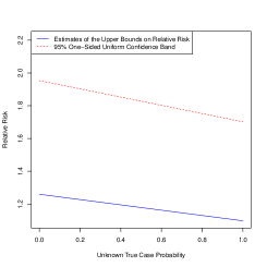
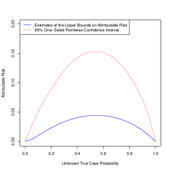
Figure 1: Causal inference on RR and AR: bounding the effects of attending private school on entering VSU

Note: The left panel shows the estimates and the 95% one-sided uniform confidence band for the upper bounds on relative risk and the right panel the estimates and the 95% one-sided pointwise confidence intervals for the upper bounds on attributable risk, as functions of the unknown true case probability, i.e., $\mathbb{P}(Y^{*}=1)$.

We now consider the methods described in section 5, i.e., causal inference on the aggregated relative and attributable risk (RR and AR, respectively) in terms of the population distribution of the covariates. We rely on the MTR and MTS assumptions to interpret our results as upper bounds. For AR, we use the same covariates as in RR. The number of the bootstrap replications was 10,000.

Figure 1 summarizes the results: the left (right) panel shows RR (AR). The case probability $p_{0}$ of entering VSU in the population is not identified in this dataset. But we can trace out the upper bounds as the value of $p_{0}$ varies between $0$ and $1$.

Consider the left panel of figure 1, i.e., RR, where we take the conservative approach and plot $\tilde{\beta}(p)=\beta(1)p+\beta(0)(1-p)$. If we take the point estimate at face value, attending private school increases the chance of entering VSU by a factor of at most 1.26. Even in terms of the confidence intervals, it seems highly unlikely that the impact is more than a factor of 2. The right panel of figure 1 shows AR. The graph shows an inverted U-shape, because $r_{\mathrm{CC}}(x,p)\Gamma_{\mathrm{CC},\mathrm{AR}}(x,p)=0$ whenever $p$ is either $0$ or $1$. The maximum point estimate of the upper bound is 0.044, while the maximum value of the confidence intervals is 0.153. Therefore, it seems highly unlikely that attending private school increases the chance of entering VSU by more than 16 percent.

None of our results require strong ignorability or the rare-disease assumption. Our conclusion of a relatively small positive effect of attending private school on entering VSU, if it exists at all, is reminiscent of existing results in labor economics that find access to private schools have only modest effects on children’s performance (see, e.g., Epple et al. 2017, MacLeod & Urquiola 2019).

6.2 Case-population sampling: joining a criminal gang

We revisit Carvalho & Soares (2016), who combine the 2000 Brazilian Census with a unique survey of drug-trafficking gangs in favelas (slums) of Rio de Janeiro; therefore, their dataset is an example of case-population sampling, i.e., our design 2. In their study, they use the method of Lancaster & Imbens (1996) to estimate a model of selection into the gang by using race, age, illiteracy, house ownership, and religiosity. They note that the five characteristics are likely to be predetermined while years of schooling may be endogenous to entry, i.e., joining the gang may lead members to drop out of school. Indeed, 90 percent of gang members are not in school, whereas 46 percent of men aged 10–25 are not in school. They find that “younger individuals, from lower socioeconomic background (black, illiterate, and from poorer families) and with no religious affiliation are more likely to join drug-trafficking gangs.”

Table 3 provides summary statistics of the sample. We regard currently not attending school as the treatment variable of interest. Unconfoundedness is not plausible because of the endogeneity of schooling that we mentioned earlier. Furthermore, it is plausible that unmeasured factors such as family support could affect both treatment and outcome. However, not being in school may increase the chance of exposure to gang-related activities, and those who chose to be in school may be the ones who care for consequences no less than those who chose not to be; therefore, the MTR and MTS follow, respectively.

Table 3: Summary Statistics of the Case-Population Sample

	(1)	(2)
	Case	Population
	Gang members	Men aged 10-25
Not in school	0.901	0.458
Black	0.269	0.142
Age	16.722	17.526
Illiterate	0.094	0.041
Owns house	0.735	0.832
No religion	0.426	0.237
Sample size	223	17175

Notes: Each entry shows the sample mean. Age is in years and all other variables are binary indicator variables. The population consists of men aged 10-25 living in Rio’s Favelas.

Table 4 presents estimation results for $\beta(y)$ and $\exp\{\beta(y)\}$, for which we control for the same covariates as Carvalho & Soares (2016). Unlike table 2, $y=0$ now corresponds to the entire population. Therefore, $\beta(0)$ itself is the log odds ratio aggregated over the population, which is the sharp upper bound on the aggregation of the log causal relative risk, i.e., $\bar{\vartheta}_{\mathrm{RR}}$. The point estimate of $\beta(0)$ is 2.71, and that of $\exp\{\beta(0)\}$ is 15.01, which suggests that the chance of those who are not in school joining a gang may be (up to) 15 times as large as that of those who are.

Table 4: Estimation results of currently not attending school on relative risk of joining a gang

	(1)	(2)
	Case	Population
	Gang members	Men aged 10-25
$\beta(y)$	2.90	2.71
95% confidence interval	[0, 3.36]	[0, 3.19]
$\exp[\beta(y)]$	18.10	15.01
95% confidence interval	[1, 28.90]	[1, 24.39]

Note: Race, age, illiteracy, house ownership, and religiosity are linearly controlled for when fitting retrospective binary logistic regression models.

Our discussion above can be supplemented by checking the causal AR. At the three points of $p_{0}\in\{0.05,0.10,0.15\}$ that Carvalho & Soares (2016) considered, the point estimates and the end-points of the uniform confidence interval (in parentheses) for the upper bound on the causal AR are 0.33 (0.43), 0.66 (0.86), and 0.99 (1), respectively. The uniform confidence band is based on 1,000 bootstrap replications. Note that the confidence band is truncated at one, because AR cannot be larger than one.

Overall, our results are suggestive of potentially large impacts of keeping young men in school in order to discourage them to participate in criminal activities. Further research based on careful study designs would be necessary to reach a more definitive answer.

6.3 Random sampling: physician’s hours

Fang & Gong (2017) construct estimates for physicians’ hours spent on Medicare beneficiaries and find that about 3 percent of physicians billed for more than 100 hours per week. They refer to these physicians as flagged physicians. Fang & Gong (2017, p. 573) state that “flagged physicians are slightly more likely to be male, non-MD, more experienced, and provide fewer E/M services. Importantly, they work in substantially smaller group practices (if at all), and have fewer hospital affiliations.” We use their study to illustrate the findings in this paper. Specifically, the outcome variable is whether a physician billed for more than 100 hours per week in either 2012 or 2013, the treatment variable is a binary indicator showing whether or not the number of group practice numbers is less than 6, which is the median size in the data, and the covariates include an indicator for male, an indicator for doctor of medicine (MD), and experience in years (cubic polynomial).

Table 5: Physician’s potential overbilling and size of the group practice

Small Group Practice Total Physician $T=0$ $T=1$ $Y=0$ (Never flagged) 38556 37348 75904 $Y=1$ (Flagged in either year) 583 1678 2261 Total 39139 39026 78165

The original dataset in Fang & Gong (2017) is updated in Fang & Gong (2020) after Matsumoto (2020) pointed out data and coding errors in the original work. In our analysis, we use the updated dataset. Table 5 summarizes the sample, which consists of 78,165 physicians who billed at least 20 hours per week.

Treating this dataset as a random sample, we extract a case-control dataset: the case sample is composed of 2,261 flagged physicians; the control sample of equal size is randomly drawn without replacement from the pool of physicians who were never flagged. Analogously, a case-population dataset is obtained by combining the case sample with a population sample of equal size that is randomly drawn without replacement from all observations and its flagged status is coded missing.

It is highly unlikely that the group practice size is exogenous conditional on a small number of covariates; hence, we rely on the monotonicity assumptions (i.e., MTR and MTS) and focus on the upper bounds on the relative and attributable risks.

Table 6: Odds Ratios

	(1)	(2)	(3)	(4)	(5)
	Random	Case-Control		Case-Population
	Sample	Sample		Sample
	All obs.	Case	Control	Case	Population
$\exp[\beta(y)]$	2.68	2.92	2.65	2.66	2.57
95% confidence interval	[1, 2.93]	[1, 3.30]	[1, 2.96]	[1, 3.01]	[1, 2.87]

Note: An indicator for male, an indicator for doctor of medicine (MD), and experience in years (cubic polynomial) are controlled for when fitting logistic regression models.

Table 6 reports the estimates of $\exp[\beta(y)]$ and their one-sided confidence intervals of $\exp[\beta(y)]$ for each sampling scheme. The lower bound is 1 because of the MTR assumption and averaging is done for a relevant population in each column. Because the proportion of the flagged physicians is less than 0.03, we invoke the rare disease assumption and regard $\exp[\beta(y)]$ as an approximation to the upper bound on RR. Although there are some noticeable differences across different columns, the estimates are similar. This is consistent with the identification result that the price to pay is less for identification of RR when we move from random sampling to outcome-dependent sampling. The story is different if we focus on AR. Table 7 shows that the upper bounds on AR under outcome-dependent sampling are much larger than those under random sampling, especially when $\bar{p}=0.1$.

Table 7: Bounds on Attributable Risk

	(1)	(2)	(3)	(4)	(5)
	Random	Case-Control		Case-Population
	Sample	Sample		Sample
		$\bar{p}=0.05$	$\bar{p}=0.10$	$\bar{p}=0.05$	$\bar{p}=0.10$
Bound estimate	0.024	0.044	0.083	0.044	0.088
95% confidence interval	[0, 0.027]	[0, 0.051]	[0, 0.095]	[0, 0.052]	[1, 0.104]

Note. The same covariates as in table 6 are controlled for. Each confidence interval is based on 1000 bootstrap replications.

Online Appendices to “Causal inference under outcome-based sampling with monotonicity assumptions”

Sung Jae Jun

Department of Economics, Pennsylvania State University

and

Sokbae Lee

Department of Economics, Columbia University and IFS

October 19, 2023

Appendix A Averaging without taking the logarithm

In the main text we followed the convention of using the logarithm of the odds ratio, and we focused on aggregated versions of the logarithm of the odds ratio, i.e., $\beta(y)=\mathbb{E}\bigl{[}\log\{\mathrm{OR}(X)\}\mid Y=y\bigr{]}$ for $y=0,1$. As a result, the aggregated version of the central causal parameter in the main text was the aggregated logarithm of relative risk, i.e., $\bar{\vartheta}_{\mathrm{RR}}:=\int_{\mathcal{X}}\log\bigl{\{}\theta_{\mathrm{RR}}(x)\bigr{\}}f_{X^{*}}(x)\ dx$.

Alternatively, one may want to proceed without taking the logarithm, which does not change the substance of our results, though the aggregate parameter of interest is now $\overline{\zeta}_{\mathrm{RR}}:=\mathbb{E}\bigl{[}\theta_{\mathrm{RR}}(X^{*})\bigr{]}$, for which we rely on

$$\zeta_{\mathrm{RR}}(y):=\int_{\mathcal{X}}\theta_{\mathrm{RR}}(x)dF_{X|Y}(x|y),\ \;\kappa_{\mathrm{RR}}(y):=\int_{\mathcal{X}}\mathrm{OR}(x)dF_{X|Y}(x|y)$$

for $y=0,1$. Again, if the MTR and MTS conditions are satisfied, then we have

$$1\leq\zeta_{\mathrm{RR}}(y)\leq\kappa_{\mathrm{RR}}(y)$$ (A.1)

under both designs 1 and 2, where the inequalities are sharp. We can construct efficient estimators of $\kappa_{\mathrm{RR}}(y)$ and carry out causal inference on $\overline{\zeta}_{\mathrm{RR}}$ by using the same idea as we described in section B.2. We do not repeat all the details for brevity.

In general, we have $\mathbb{E}\{\log\mathrm{OR}(X^{*})\}\leq\log\mathbb{E}\{\mathrm{OR}(X^{*})\}$ by Jensen’s inequality. Therefore, an average of the log odds ratio is less likely to be affected unduly by outliers than that of the odds ratio itself. This seems to be another merit in using the logarithm of the odds ratio in addition to the usual advantage that it corresponds to the coefficients of the treatment variable when a parametric logistic model is used.

Appendix B Efficient Estimation of $\beta(y)$

In this section, we discuss efficient estimation of $\beta(y):=\mathbb{E}\bigl{[}\log\{\mathrm{OR}(X)\}\mid Y=y\bigr{]}$ for $y=0,1$. For this purpose, we point out that the sample consists of independent and identically distributed copies of $(Y,T,X)$: the sampling designs affect the distribution of $(Y,T,X)$ and its relationship with that of $(Y^{*},T^{*},X^{*})$. Therefore, all regularity conditions and results in this section will be presented in terms of the observed variables $(Y,T,X)$, and hence the regularity conditions are testable in principle.

B.1 The efficient influence function

We first derive the semiparametric efficiency bound. We start with the following assumptions for regularity.

Assumption A.1 (Bounded Probabilities).

There is a constant $\varepsilon>0$ such that for each $y=0,1$, $\varepsilon\leq\mathbb{P}(T=1\mid X,Y=y)\leq 1-\varepsilon$ and $\varepsilon\leq\mathbb{P}(Y=1\mid X)\leq 1-\varepsilon$ almost surely.

Assumption A.2 (Regular Distribution).

The distribution function $F_{X|Y}$ has a probability density $f_{X|Y}$ that satisfies $0<f_{X|Y}(x\mid y)<\infty$ for all $x\in\mathcal{X}$ and $y=0,1$.

Assumption A.1 is slightly stronger than what we need to derive the efficient influence function, but it is useful to ensure that all the population quantities given below are well-defined without spelling out all the conditions. Assumption A.2 focuses on the case where $X$ is continuous, but this is only for the sake of notational simplicity.

Under Bernoulli sampling, the likelihood of a single observation $(Y,T,X)$ can be expressed as a mixture of two binary likelihoods, from which we first have the following lemma.

Lemma A.1.

Consider the Bernoulli sampling scheme of design 1 or design 2. The tangent space can be represented by the set of functions of the following form:

$$s(Y,T,X)=(1-Y)\Bigl{[}a_{0}(X)+\bigl{\{}T-\mathbb{P}(T=1\mid X,Y=0)\bigr{\}}b_{0}(X)\Bigr{]}\\ +Y\Bigl{[}a_{1}(X)+\bigl{\{}T-\mathbb{P}(T=1\mid X,Y=1)\bigr{\}}b_{1}(X)\Bigr{]},$$

where the functions $a_{y}$ and $b_{y}$ are such that $\mathbb{E}\{a_{y}(X)\mid Y=y\}=0$ and $\mathbb{E}\{s^{2}(Y,T,X)\}<\infty$ for each $y=0,1$.

By direct calculation, as in Hahn (1998), we can show that $\beta(y)$ is pathwise differentiable along regular parametric submodels in the sense of Newey (1990, 1994). Further, it turns out that the pathwise derivative is an element of the tangent space presented in lemma A.1, from which we can obtain the semiparametric efficiency bound for $\beta(y)$. The following theorem presents this result. Let

$$w(X):=\frac{f_{X|Y}(X\mid 0)}{f_{X|Y}(X\mid 1)}=\frac{h_{0}}{1-h_{0}}\frac{\mathbb{P}(Y=0\mid X)}{\mathbb{P}(Y=1\mid X)},$$ (A.2)

where the second equality is by the Bayes rule. Further, for $y=0,1$, define

$$\Delta_{y}(Y,T,X):=\frac{Y^{y}(1-Y)^{1-y}\{T-\mathbb{P}(T=1\mid X,Y=y)\}}{\mathbb{P}(T=1\mid X,Y=y)\{1-\mathbb{P}(T=1\mid X,Y=y)\}}.$$

Theorem A.1.

Suppose that assumptions A, A.1 and A.2 hold and that we have a sample by Bernoulli sampling. Then, for $y=0,1$, $\beta(y)$ is pathwise differentiable and its pathwise derivative is given by

$$F_{y}(Y,T,X)=\frac{Y^{y}(1-Y)^{1-y}}{h_{0}^{y}(1-h_{0})^{1-y}}\Bigl{\{}\log\mathrm{OR}(X)-\beta(y)\Bigr{\}}\\ -\frac{\Delta_{0}(Y,T,X)}{(1-h_{0})w(X)^{y}}+\frac{w(X)^{1-y}\Delta_{1}(Y,T,X)}{h_{0}}.$$

Further, $F_{y}$ is an element of the tangent space, and therefore, the semiparametric efficiency bound for $\beta(y)$ is given by $\mathbb{E}\bigl{\{}F_{y}^{2}(Y,T,X)\bigr{\}}$.

Theorem A.1 implies that the asymptotic variance of a $\sqrt{n}$–consistent and asymptotically linear estimator of $\beta(y)$ should be at least $\mathbb{E}\{F_{y}^{2}(Y,T,X)\}$ by Theorem 2.1 of Newey (1994). The first term that appears in $F_{y}(Y,T,X)$ has mean zero, because

$$\mathbb{E}\Biggl{[}\frac{Y^{y}(1-Y)^{1-y}}{h_{0}^{y}(1-h_{0})^{1-y}}\Bigl{\{}\log\mathrm{OR}(X)-\beta(y)\Bigr{\}}\Biggr{]}=\mathbb{E}\bigl{\{}\log\mathrm{OR}(X)-\beta(y)\ \big{|}\ Y=y\bigr{\}}=0.$$ (A.3)

The other terms in $F_{y}(Y,T,X)$ are for adjustment to address the effect of first step nonparametric estimation of $\log\mathrm{OR}(X)$ via $\mathbb{P}(T=1\mid X=x,Y=y)$.

We remark that the efficiency bound does not change even if $h_{0}$ is unknown, as long as the distribution of $(T,X)$ given $Y=y$ does not depend on $h_{0}$. This point can be seen as follows. Suppose that $h_{0}$ is unknown and that the distribution of $(T,X)$ given $Y=y$ does not depend on $h_{0}$. Then, the log-likelihood of a regular parametric submodel as we perturb the conditional distributions of $T,X$ given $Y=y$ can be written as

$$\ell(h,\gamma;Y,T,X)=Y\{\log h+\ell_{1}(\gamma;T,X)\}+(1-Y)\{\log(1-h)+\ell_{0}(\gamma;T,X)\},$$

where $\ell_{y}(\gamma;T,X)=\log\mathbb{P}(T,X|Y=y;\gamma)$ is the log-likelihood of the conditional distribution of $T,X$ given $Y=y$ along a parametric perturbation represented by $\gamma$ (with the true vale at $\gamma_{0}$). Here, $\ell_{y}(\gamma;T,X)$ does not depend on $h$ by assumption. Therefore, the information matrix is block diagonal, and the score along the $\gamma$–dimension in this setup is the same as the score under the assumption that $h_{0}$ is known. Since the new tangent space is obtained by a linear span of the scores along the $h$ and $\gamma$ dimensions, it is always a larger space than the tangent space we obtained under the assumption that $h_{0}$ is known.

Now, note that the parameter $\beta(y)$ depends only on $\mathbb{P}(T,X\mid Y=1),\mathbb{P}(T,X\mid Y=0)$, and $f(X\mid Y=y)$, none of which depend on $h_{0}$ by assumption. Therefore, only the perturbation along the $\gamma$–dimension will affect $\beta(y)$, which means that the perturbed parameter $\beta(y;h,\gamma)$ along $(h,\gamma)$ will be just the same as $\beta(y;\gamma)$. Therefore, the pathwise derivative of $\beta(y)$ stays the same whether $h_{0}$ is known or not.

Since we already showed that the pathwise derivative of $\beta(y)$ is contained in the tangent space we obtained under the assumption that $h_{0}$ is known, it must be included in the new tangent space as well. Therefore, the pathwise derivative itself is again the efficient influence function, which is the same whether $h_{0}$ is known or not. This point can be seen from a slightly different angle based on the moment condition and block diagonality of the information. See section B.2 for more details.

B.2 An efficient estimation algorithm

Efficient estimators of $\beta(y)$ for $y=0,1$ can be constructed in multiple ways. The most straightforward approach is using the moment condition

$$\mathbb{E}\left\{\frac{Y^{y}(1-Y)^{1-y}\{\log\mathrm{OR}(X)-\beta(y)\}}{h_{0}^{y}(1-h_{0})^{1-y}}\right\}=0,$$ (A.4)

where we plug in a nonparametric estimator of $\mathrm{OR}(x)$. A resulting estimator will be $\sqrt{n}$-consistent, asymptotically linear, and semiparametrically efficient under suitable conditions. Below we propose a simple algorithm that implements this idea, for which we use sieve logistic estimators for the first step nonparametric estimation.

Suppose that we have an i.i.d. sample, $\bigl{\{}(Y_{i},T_{i},X_{i}):i=1,\dots,n\bigr{\}}$: this is not an i.i.d. sample of $(Y_{i}^{*},T_{i}^{*},X_{i}^{*})$. Throughout the discussion, we assume that $h_{0}$ is known; otherwise, we can use $\hat{h}:=\sum_{i=1}^{n}Y_{i}/n$ instead, which does not affect the asymptotic variance (or equivalently the efficiency bound), provided that the distribution of $(T,X)$ given $Y=y$ does not depend on $h_{0}$. Indeed, if $\mathrm{OR}(x)$ does not depend on $h_{0}$, then we can index the moment condition in equation A.4 along parametric submodels as $\mathbb{E}\{m_{y}(h_{0},\gamma_{0},\beta(y);Y,X)\}=0$, where

$$m_{y}(h,\gamma,\beta;Y,X):=\frac{Y^{y}(1-Y)^{1-y}\{\log\mathrm{OR}(X;\gamma)-\beta\}}{h^{y}(1-h)^{1-y}}.$$

Then, some simple algebra shows that $\mathbb{E}[\partial m_{y}\{h,\gamma_{0},\beta(1);Y,X\}/\partial h|_{h=h_{0}}]=0$. Therefore, it is only the estimation of $\gamma_{0}$, not the estimation of $h_{0}$, that matters for the variance of the estimator of $\beta(y)$. But we already argued at the end of section B.1 that the information along $h$ and $\gamma$ is block diagonal.

In order to estimate $\mathrm{OR}(x)$ nonparametrically in the first step, we consider infinite dimensional (retrospective) logistic regression: i.e., for $y=0,1$,

$$\mathbb{P}(T=1\mid X=x,Y=y)=\frac{\exp\left\{\sum_{j=1}^{\infty}\phi_{j}(x)\mu_{j,y}\right\}}{1+\exp\left\{\sum_{j=1}^{\infty}\phi_{j}(x)\mu_{j,y}\right\}},$$ (A.5)

where $\{\phi_{j}:j=1,2,\ldots\}$ is a series of basis functions and $\{\mu_{j,y}:j=1,2,\ldots\}$ is a series of unknown coefficients for each $y=0,1$. It then follows that $\log\mathrm{OR}(x)=\sum_{j=1}^{\infty}\phi_{j}(x)(\mu_{j,1}-\mu_{j,0})$, from which we obtain

$$\beta(y)\approx\sum_{j=1}^{J_{n}}\int_{\mathcal{X}}\phi_{j}(x)dF_{X|Y}(x|y)\left(\mu_{j,1}-\mu_{j,0}\right),$$ (A.6)

provided that $J_{n}$ diverges as $n$ increases. Equation A.6 suggests the following two-step sieve estimation strategy:

1. In the first step, for each $y=0,1$, estimate $\{\mu_{j,y}:y=0,1\;j=1,\ldots,J_{n}\}$ by logistic regression of $T_{i}$ on $\{\phi_{j}(X_{i}):j=1,\ldots,J_{n}\}$ with the $Y_{i}=y$ sample.

2. In the second step, construct a sample analog of equation A.6: i.e.,

   $$\widehat{\beta}(y):=\sum_{j=1}^{J_{n}}\int_{\mathcal{X}}\phi_{j}(x)d\widehat{F}_{X|Y}(x|y)\left(\widehat{\mu}_{j,1}-\widehat{\mu}_{j,0}\right),$$ (A.7)

   where $\widehat{\mu}_{j,y}$’s are sieve logit estimates from the first step, and

   $$\int_{\mathcal{X}}\phi_{j}(x)d\widehat{F}_{X|Y}(x|y)=\frac{\sum_{i=1}^{n}Y_{i}^{y}(1-Y_{i})^{y}\phi_{j}(X_{i})}{\sum_{i=1}^{n}Y_{i}^{y}(1-Y_{i})^{y}}.$$

Since we use retrospective regression as shown in equation A.5, we call the estimator defined in (A.7) the retrospective sieve logistic estimator of $\beta(y)$ for $y=0,1$. It can be computed using standard software for logistic regression, as described in algorithm 1.

Input: $\{(Y_{i},T_{i},X_{i}):i=1,\ldots,n\}$, tuning parameter $J_{n}$ and basis functions $\{\phi_{j}(\cdot):j=1,\ldots,J_{n}\}$

Output: estimate of $\beta(1)$ and its standard error

1

2Construct $\{\phi_{1}(X_{i}),\ldots,\phi_{J_{n}}(X_{i}):i=1,\ldots,n\}$, where an intercept term is excluded in $\phi_{j}$’s;

3

4For each $j=1,\ldots,J_{n}$, compute the empirical mean of $\phi_{j}(X_{i})$ using only the case sample ($Y_{i}=1$) and construct the demeaned version, say $\varphi_{j}(X_{i})$, of $\phi_{j}(X_{i})$;

5

6Run a logistic regression of $T_{i}$ on the following regressors: an intercept term, $Y_{i}$, $\varphi_{j}(X_{i}),j=1,\ldots,J_{n},$ and interactions between $Y_{i}$ and $\varphi_{j}(X_{i}),j=1,\ldots,J_{n},$ using standard software;

7Read off the estimated coefficient for $Y_{i}$ and its standard error

Algorithm 1 Retrospective Sieve Logistic Estimator of $\beta(1)$

The procedure described in algorithm 1 achieves the first step by running a combined logistic regression of $T_{i}$ on $Y_{i}$, the sieve basis terms and the interactions between $Y_{i}$ and the sieve basis terms. This is first-order equivalent since $Y_{i}$ is binary and full interaction terms are included. For the second step, instead of evaluating the right-hand side of equation A.7 after logistic regression, $\phi_{j}(X_{i})$’s are demeaned first using only the case sample so that the resulting coefficient for $Y_{i}$ is first-order equivalent to the estimator defined in equation A.7. The advantage of the formulation in algorithm 1 is that the standard error of $\widehat{\beta}(1)$ can be read off directly from standard software without any further programming. It is straightforward to modify algorithm 1 for estimating $\beta(0)$. One has to compute the empirical mean of $\phi_{j}(X_{i})$ using only the control sample ($Y_{i}=0$) for the demeaning step.

It is not difficult to work out formal asymptotic properties of our proposed sieve estimator in view of the well-established literature on two-step sieve estimation (see, e.g., Ai & Chen 2003, 2012, Ackerberg et al. 2014, among many others). Since this is now well understood in the literature, we omit details for brevity of the paper. Appendix C reports the results of a small Monte Carlo experiment that illustrates the finite-sample performance of the proposed estimators of $\beta(1)$ and $\beta(0)$.

Appendix C Monte Carlo Experiments

In this section, we report the results of a small Monte Carlo experiment. A case-control sample is generated from

$$X\mid Y=y\sim\mathbb{N}(\mu^{(y)},\Sigma^{(y)})\quad\text{and}\quad\mathbb{P}(T=1\mid X=x,Y=y)=G(\alpha_{0}^{(y)}+X^{\mathchoice{\raisebox{0.75346pt}{$\displaystyle\intercal$}}{\raisebox{0.75346pt}{$\textstyle\intercal$}}{\raisebox{0.75346pt}{$\scriptstyle\intercal$}}{\raisebox{0.75346pt}{$\scriptscriptstyle\intercal$}}}\alpha_{1}^{(y)}),$$

where $G(u)=\exp(u)/\{1+\exp(u)\}$, $\alpha_{0}^{(y)}$, $\alpha_{1}^{(y)}$, $\mu^{(y)}$ and $\Sigma^{(y)}$ are parameters that may depend on $y=0,1$. In simulations we focus on estimating $\beta(y)$ that can now be expressed as $\beta(y)=(\alpha_{0}^{(1)}-\alpha_{0}^{(0)})+\mathbb{E}(X|Y=y)^{\mathchoice{\raisebox{0.75346pt}{$\displaystyle\intercal$}}{\raisebox{0.75346pt}{$\textstyle\intercal$}}{\raisebox{0.75346pt}{$\scriptstyle\intercal$}}{\raisebox{0.75346pt}{$\scriptscriptstyle\intercal$}}}(\alpha_{1}^{(1)}-\alpha_{1}^{(0)})$.

With the dimension of $X$ equal to $d_{x}=5$, the parameter values are specified as follows: $\mu^{(1)}=(1,\ldots,1)^{\mathchoice{\raisebox{0.75346pt}{$\displaystyle\intercal$}}{\raisebox{0.75346pt}{$\textstyle\intercal$}}{\raisebox{0.75346pt}{$\scriptstyle\intercal$}}{\raisebox{0.75346pt}{$\scriptscriptstyle\intercal$}}}$, $\mu^{(0)}=(0,\ldots,0)^{\mathchoice{\raisebox{0.75346pt}{$\displaystyle\intercal$}}{\raisebox{0.75346pt}{$\textstyle\intercal$}}{\raisebox{0.75346pt}{$\scriptstyle\intercal$}}{\raisebox{0.75346pt}{$\scriptscriptstyle\intercal$}}}$, and $\Sigma^{(y)}=\Sigma$ for $y=0,1$, where the $(j,k)$ element of $\Sigma$ is $\Sigma_{j,k}=\rho^{|j-k|}$ and $\rho=0.5$; $\alpha_{0}^{(1)}=0.5$, $\alpha_{1}^{(1)}=(1,1,0,0,0)^{\mathchoice{\raisebox{0.75346pt}{$\displaystyle\intercal$}}{\raisebox{0.75346pt}{$\textstyle\intercal$}}{\raisebox{0.75346pt}{$\scriptstyle\intercal$}}{\raisebox{0.75346pt}{$\scriptscriptstyle\intercal$}}}$, $\alpha_{0}^{(0)}=0$, $\alpha_{1}^{(0)}=(0,0,1,1,0)^{\mathchoice{\raisebox{0.75346pt}{$\displaystyle\intercal$}}{\raisebox{0.75346pt}{$\textstyle\intercal$}}{\raisebox{0.75346pt}{$\scriptstyle\intercal$}}{\raisebox{0.75346pt}{$\scriptscriptstyle\intercal$}}}$. In this design we have $\beta(1)=\beta(0)=0.5$.

In each Monte Carlo replication, we simulate 1,000 observations separately for both $Y=0$ and $Y=1$ samples (that is, the total sample size is 2,000 and $\hat{h}=0.5$). There are 1,000 Monte Carlo replications.

Table A.1: Results of Monte Carlo Experiments

	$\beta(1)$		$\beta(0)$
	parametric	sieve	parametric	sieve
Mean Bias	0.011	0.070	0.005	0.046
Median Bias	0.012	0.086	-0.001	0.042
RMSE	0.057	0.167	0.033	0.067
Mean AD	0.191	0.330	0.145	0.206
Median AD	0.160	0.283	0.119	0.173
Cov. Prob.	0.944	0.962	0.952	0.962

Note: RMSE stands for the root mean squared error and AD refers to absolute deviation. Cov. Prob. is the coverage probability of the one-sided 95% confidence interval. The results are based on 1,000 Monte Carlo repetitions.

We consider two estimators: (i) a retrospective parametric logistic estimator that uses $X$ as covariates and (ii) a retrospective sieve logistic estimator that uses the linear, quadratic and interaction terms of $X$ as covariates (that is, $2d_{x}+d_{x}(d_{x}-1)/2=20$ covariates all together). Table A.1 summarizes the results of the Monte Carlo experiments. Not surprisingly, the parametric estimator performs better for both $\beta(1)$ and $\beta(0)$. It shows almost no bias and small root mean squared errors and absolute deviations. Its coverage probability is close to the nominal 95%. The sieve estimator exhibits some positive biases but its performance is overall satisfactory.

Appendix D Inferential Details

In this section, we provide details that are omitted in section 5. We first show equation 8. Let $\bar{\beta}(y):=\hat{\beta}(y)-\beta(y)$ for $y=0,1$, where $\hat{\beta}(y)$ is an asymptotically normal estimator of $\beta(y)$ with the standard error equal to $\hat{s}(y)$. Note that

$$\mathbb{B}:=\inf_{p\in[0,1]}\bigl{\{}p\bar{\beta}(1)+(1-p)\bar{\beta}(0)\bigr{\}}=\min\{\bar{\beta}(1),\bar{\beta}(0)\}.$$

Therefore,

$$\mathbb{P}\{\mathbb{B}\leq-u(1-\alpha)\}\leq\sum_{y=0}^{1}\mathbb{P}\{\bar{\beta}(y)\leq-u(1-\alpha)\}\leq\alpha/2+\alpha/2.$$

This procedure can be easily modified when assumption F with $\bar{p}<1$ is adopted.

We remark that the asymptotic coverage rate in equation 8 is conservative. Achieving the asymptotically exact coverage rate requires that we use the limiting distribution of $\min\{\bar{\beta}(1),\bar{\beta}(0)\}$, which is not normal and is not readily available from the estimation algorithm given in Section B.2. Also, if one wants to directly use the nonlinear function $\mathcal{C}_{\mathrm{CC},\mathrm{RR}}(p)$, then the bootstrap-based algorithm described in algorithm 2 can be used: algorithm 2 focuses on $\mathcal{C}_{\mathrm{CC},\mathrm{AR}}$, but its modification for $\mathcal{C}_{\mathrm{CC},\mathrm{RR}}$ is straightforward.

Input: $\{(Y_{i},T_{i},X_{i}):i=1,\ldots,n\}$, the number ($B$) of bootstrap replications, the coverage probability ($1-\alpha$) of the confidence interval, the upper bound ($\bar{p}$) on the unknown true case probability

1

Output: point estimates $\widehat{\mathcal{C}}_{\mathrm{CC},\mathrm{AR}}(p)$ of the upper bounds on causal attributable risk and the upper end points of the one-sided pointwise bootstrap confidence intervals $q_{(1-\alpha)}^{*}(p)$ for $p\in[0,\bar{p}]$

2

3

4Construct a grid $\mathcal{P}:=\{p_{0},p_{1},\ldots,p_{J}\}$ of $[0,\bar{p}]$, where $0=p_{0}<p_{1}<\dots<p_{J}=\bar{p}$;

5For each $p\in\mathcal{P}$, evaluate sample analogs $\widehat{\mathcal{C}}_{\mathrm{CC},\mathrm{AR}}(p)$ of $\mathcal{C}_{\mathrm{CC},\mathrm{AR}}(p):=p\Psi_{\mathrm{CC},\mathrm{AR}}(p,1)+(1-p)\Psi_{\mathrm{CC},\mathrm{AR}}(p,0)$; in this step, we need to compute retrospective estimates of $\Pi(t\mid y,X_{i})$ for $t=0,1,\ y=0,1$ as well as prospective estimates of $\mathbb{P}(Y=1\mid X_{i})$, because $\Psi_{\mathrm{CC},\mathrm{AR}}(p,y)$ depends on $r_{\mathrm{CC}}(x,p)$ as its definition in equation 3 shows;

6For each bootstrap replication $b=1,\ldots,B$, generate a bootstrap sample $\{(Y_{i}^{*,b},T_{i}^{*,b},X_{i}^{*,b}):i=1,\ldots,n\}$, and obtain a bootstrap estimate $\widehat{\mathcal{C}}^{*,b}_{\mathrm{CC},\mathrm{AR}}(p)$ for each $p\in\mathcal{P}$;

7For each $p\in\mathcal{P}$, compute

$$\mu^{*}(p):=\frac{1}{B}\sum_{b=1}^{B}\mathbb{1}\left\{\widehat{\mathcal{C}}^{*,b}_{\mathrm{CC},\mathrm{AR}}(p)\leq\widehat{\mathcal{C}}_{\mathrm{CC},\mathrm{AR}}(p)\right\},$$

where $\mathbb{1}\{\cdot\}$ is the usual indicator function;

8For each $p\in\mathcal{P}$, obtain $\nu^{*}(p):=\Phi\left[\Phi^{-1}(1-\alpha)+2\Phi^{-1}\{\mu^{*}(p)\}\right]$, where $\Phi(\cdot)$ is the cumulative distribution function of the standard normal random variable;

9For each $p\in\mathcal{P}$, compute the $\nu^{*}(p)$ empirical quantile of $\widehat{\mathcal{C}}^{*,b}_{\mathrm{CC},\mathrm{AR}}(p)$, say $q_{(1-\alpha)}^{*}(p)$, as the $(1-\alpha)$ one-sided pointwise bootstrap confidence interval

Algorithm 2 Causal Inference on $\bar{\vartheta}_{\mathrm{AR}}$ Using Case-Control Samples

We now turn to $\bar{\vartheta}_{\mathrm{AR}}$. In the case-population case, we use the fact that $\Psi_{\mathrm{CP},\mathrm{AR}}(p)$ has a simple linear form such as $\Psi_{\mathrm{CP},\mathrm{AR}}(p):=p\xi_{\mathrm{CP}}$, where

$$\xi_{\mathrm{CP}} :=\mathbb{E}\biggl{\{}\frac{(1-h_{0})}{h_{0}}\frac{\mathbb{P}(Y=1\mid X=x)}{\mathbb{P}(Y=0\mid X=x)}\Gamma_{\mathrm{CP},\mathrm{AR}}(X,0)\ \Big{|}\ Y=0\biggr{\}},$$

$$\Gamma_{\mathrm{CP},\mathrm{AR}}(x,0) =\sum_{j=0}^{1}\frac{(-1)^{j+1}\Pi(j\mid 1,x)}{\Pi(j\mid 0,x)}.$$

Therefore, a one-side confidence band that is uniform in $p$ can be constructed as

$$p\in[0,1]\mapsto\bigl{[}0,\ p\{\hat{\xi}_{\mathrm{CP}}+u_{\mathrm{AR},\mathrm{CP}}(1-\alpha)\}\bigr{]},$$

where $\hat{\xi}_{\mathrm{CP}}$ is an estimator of $\xi_{\mathrm{CP}}$, and $-u_{\mathrm{AR},\mathrm{CP}}(1-\alpha)$ is, for instance, the bootstrap $\alpha$-quantile of $\hat{\xi}_{\mathrm{CP}}-\xi_{\mathrm{CP}}$. We note here that the asymptotic validity of the nonparametric bootstrap in two-step semiparametric models is a well-studied topic (e.g., Chen et al. 2003). However, in practice, the naïve bootstrap may suffer from a finite sample bias, because ratios of probabilities need to be estimated in the first step. To mitigate this issue, we recommend using Efron (1982)’s bias-corrected one-sided percentile interval to obtain $u_{\mathrm{AR},\mathrm{CP}}(1-\alpha)$: see the bootstrap procedure we describe in algorithm 2. Finally, it is straightforward to adopt assumption F by restricting attention to $p\in[0,\bar{p}]$.

Computational details for the case of case-control sampling are given in algorithm 2.

Appendix E Proofs

It is worth noting that our big picture arguments consist of two parts. In Part 1, we suppose that the distribution of $(Y^{*},T^{*},X^{*})$ were known, and we obtain the sharp identified intervals on the parameters of interest in terms of the distribution of $(Y^{*},T^{*},X^{*})$. In Part 2, we show that the bounds obtained in Part 1 can be equivalently expressed in terms of the distribution of $(Y,T,X)$ and $p_{0}=\mathbb{P}(Y^{*})$. Therefore, finding the final sharp identified bounds in terms of the distribution of $(Y,T,X)$ becomes just a matter of dealing with the unknown value of $p_{0}$, which can be taken care of by a simple continuity argument.

In this section, we present all proofs.

E.1 Auxiliary Results

We first summarize all the restrictions imposed by assumptions D and E. The conditional probability mass function of $\bigl{(}Y^{*}(0),Y^{*}(1),T^{*}\bigr{)}$ given $X^{*}=x$ can be tabulated as in table A.2 under assumption D.

Table A.2: The distribution of $\bigl{(}Y^{*}(0),Y^{*}(1),T^{*}\bigr{)}$ given $X^{*}=x$ under the MTR

$\bigl{(}Y^{*}(0),Y^{*}(1)\bigr{)}=$	$(0,0)$	$(0,1)$	$(1,1)$	$(1,0)$
$T^{*}=0$	$q_{0}(x)$	$q_{2}(x)$	$q_{4}(x)$	$0$
$T^{*}=1$	$q_{1}(x)$	$q_{3}(x)$	$q_{5}(x)$	$0$
Prob Restrictions	$\sum_{j=0}^{5}q_{j}(x)=1$
	$0\leq q_{j}(x)\leq 1$ for $j=0,\dots,5$

Further, assumption E imposes additional restrictions on the $q_{j}$ functions such that

$$\frac{q_{5}(x)}{q_{1}(x)+q_{3}(x)+q_{5}(x)} \geq\frac{q_{4}(x)}{q_{0}(x)+q_{2}(x)+q_{4}(x)},$$ (A.8)

$$\frac{q_{3}(x)+q_{5}(x)}{q_{1}(x)+q_{3}(x)+q_{5}(x)} \geq\frac{q_{2}(x)+q_{4}(x)}{q_{0}(x)+q_{2}(x)+q_{4}(x)}.$$

Now, $q_{j}(x)$’s are all otherwise unrestricted under assumptions D and E.

Lemma A.2.

Suppose that assumptions A, B, D and E hold. Suppose that the distribution of $(Y^{*},T^{*},X^{*})$ is known. For all $(t,x)\in\{0,1\}\times\mathcal{X}$,

$$(-1)^{t}\bigl{[}\mathbb{P}\{Y^{*}(t)=1\mid X^{*}=x\}-\mathbb{P}(Y^{*}=1\mid X^{*}=x)\bigr{]}\leq 0,$$

$$(-1)^{t}\bigl{[}\mathbb{P}\{Y^{*}(t)=1\mid X^{*}=x\}-\mathbb{P}(Y^{*}=1\mid T^{*}=t,X^{*}=x)\bigr{]}\geq 0,$$

and the bounds are sharp.

Proof.

Assumption B ensures that $0<\mathbb{P}(T^{*}=t\mid X^{*}=x)<1$, and hence $\mathbb{P}(Y^{*}=1\mid T^{*}=t,X^{*}=x)$ is well-defined. Below we will write $q_{j}(x)$ for $j=0,1,2,\cdots,5$ for the probabilities that describe the distribution of $\bigl{(}Y^{*}(0),Y^{*}(1),T^{*})$ given $X^{*}=x$: see our discussion in the beginning of the current section.

For $(y,t)\in\{0,1\}^{2}$, let $\Delta_{yt}(x):=\mathbb{P}(Y^{*}=y,T^{*}=t\mid X^{*}=x)$. When the distribution of $(Y^{*},T^{*})$ given $X^{*}=x$ is given, we know that under assumption D,

$$q_{0}(x)+q_{2}(x) =\Delta_{00}(x),$$

$$q_{4}(x) =\Delta_{10}(x),$$

$$q_{1}(x) =\Delta_{01}(x),$$

$$q_{3}(x)+q_{5}(x) =1-\Delta_{00}(x)-\Delta_{10}(x)-\Delta_{01}(x),$$

where $\sum_{j=0}^{5}q_{j}(x)=1$. Therefore, two of the $q_{j}(x)$’s are undetermined under assumption D. Specifically, since $q_{5}(x)=1-\sum_{j=0}^{4}q_{j}(x)$, dropping the last equation for its redundancy yields

$$q_{1}(x)=\Delta_{01}(x),\quad q_{2}(x)=\Delta_{00}(x)-q_{0}(x),\quad q_{4}(x)=\Delta_{10}(x),$$ (A.9)

and $q_{5}(x)=\Delta_{11}(x)-q_{3}(x)$: i.e., we have used $q_{0}(x)$ and $q_{3}(x)$ as the undetermined ones here. Since all the $q_{j}(x)$’s are between $0$ and $1$, $q_{0}(x)$ and $q_{3}(x)$ must satisfy $0\leq q_{0}(x)\leq\Delta_{00}(x)$ and $0\leq q_{3}(x)\leq\Delta_{11}(x)$: they are otherwise unrestricted under assumption D.

Now, assumption E imposes additional restrictions on $q_{0}(x),q_{3}(x)$: i.e., the inequalities in equation A.8 can now be written as

$$\frac{\Delta_{11}(x)-q_{3}(x)}{\Delta_{01}(x)+\Delta_{11}(x)} \geq\frac{\Delta_{10}(x)}{\Delta_{00}(x)+\Delta_{10}(x)},$$ (A.10)

$$\frac{\Delta_{11}(x)}{\Delta_{01}(x)+\Delta_{11}(x)} \geq\frac{\Delta_{00}(x)+\Delta_{10}(x)-q_{0}(x)}{\Delta_{00}(x)+\Delta_{10}(x)}.$$

Therefore, under assumptions D and E, we have

$$0\leq q_{3}(x)\leq\Delta_{11}(x)-\frac{\Delta_{10}(x)\{\Delta_{01}(x)+\Delta_{11}(x)\}}{\Delta_{00}(x)+\Delta_{10}(x)},$$ (A.11)

$$\Delta_{00}(x)+\Delta_{10}(x)-\frac{\Delta_{11}(x)\{\Delta_{00}(x)+\Delta_{10}(x)\}}{\Delta_{01}(x)+\Delta_{11}(x)}\leq q_{0}(x)\leq\Delta_{00}(x).$$ (A.12)

These are the only restrictions that assumptions D and E impose on $q_{0}(x)$ and $q_{3}(0)$ when we know the distribution of $(Y^{*},T^{*})$ given $X^{*}=x$. Note that the upper bound in equation A.11 is equal to

$$\mathbb{P}(Y^{*}=1,T^{*}=1\mid X^{*}=x)-\mathbb{P}(T^{*}=1\mid X^{*}=x)\mathbb{P}(Y^{*}=1\mid T^{*}=0,X^{*}=x)$$

$$=\mathbb{P}(T^{*}=1\mid X^{*}=x)\bigl{\{}\mathbb{P}(Y^{*}=1\mid T^{*}=1,X^{*}=x)-\mathbb{P}(Y^{*}=1\mid T^{*}=0,X^{*}=x)\bigr{\}},$$

which is trivially no greater than $1$ and is no smaller than $0$ by assumptions D and E, because

$$\mathbb{P}(Y^{*}=1\mid T^{*}=1,X^{*}=x)-\mathbb{P}(Y^{*}=1\mid T^{*}=0,X^{*}=x)$$ (A.13)

$$=\mathbb{P}\{Y^{*}(1)=1\mid T^{*}=1,X^{*}=x\}-\mathbb{P}\{Y^{*}(0)=1\mid T^{*}=0,X^{*}=x\}$$

$$\geq\mathbb{P}\{Y^{*}(1)=1\mid T^{*}=1,X^{*}=x\}-\mathbb{P}\{Y^{*}(1)=1\mid T^{*}=0,X^{*}=x\}\geq 0.$$

The lower bound in equation A.12 is equal to

$$\mathbb{P}(T^{*}=0\mid X^{*}=x)-\mathbb{P}(T^{*}=0\mid X^{*}=x)\mathbb{P}(Y^{*}=1\mid T^{*}=1,X^{*}=x),$$

which is trivially no smaller than $0$ and is no greater than $\Delta_{00}(x)$ by assumptions D and E, because

$$1-\mathbb{P}(Y^{*}=1\mid T^{*}=1,X^{*}=x)\leq 1-\mathbb{P}(Y^{*}=1\mid T^{*}=0,X^{*}=x)$$

as we have shown in equation A.13.

Below we calculate the sharp bounds on $\mathbb{P}\{Y^{*}(t)=1\mid X^{*}=x\}$ for $t=0,1$ by expressing them as a function of $q_{0}(x),q_{3}(x)$ and finding their maxima and minima subject to the constraints in equations A.11 and A.12. First, consider the case of $t=1$:

$$\mathbb{P}\{Y^{*}(1)=1\mid X^{*}=x\} =\mathbb{P}\{Y^{*}(1)=1,T^{*}=0\mid X^{*}=x\}+\Delta_{11}(x)$$

$$=q_{2}(x)+q_{4}(x)+\Delta_{11}(x)$$

$$=\Delta_{00}(x)+\Delta_{10}(x)+\Delta_{11}(x)-q_{0}(x).$$

Therefore, by using equation A.12, we can find the sharp bounds on $\mathbb{P}\{Y^{*}(1)=1\mid X^{*}=x\}$. Specifically, when $q_{0}(x)=\Delta_{00}(x)$, we have the sharp lower bound on $\mathbb{P}\{Y^{*}(1)=1\mid X^{*}=x\}$, which is equal to

$$\Delta_{00}(x)+\Delta_{10}(x)+\Delta_{11}(x)-\Delta_{00}(x)=\mathbb{P}(Y^{*}=1\mid X^{*}=x).$$

For the sharp upper bound on $\mathbb{P}\{Y^{*}(1)=1\mid X^{*}=x\}$, we set $q_{0}(x)$ to its lower bound in equation A.12, which yields

$$\Delta_{00}(x)+\Delta_{10}(x)+\Delta_{11}(x)-\Delta_{00}(x)-\Delta_{10}(x)+\frac{\Delta_{11}(x)\{\Delta_{00}(x)+\Delta_{10}(x)\}}{\Delta_{01}(x)+\Delta_{11}(x)}$$

$$=\Delta_{11}(x)\Bigl{\{}1+\frac{\Delta_{00}(x)+\Delta_{10}(x)}{\Delta_{01}(x)+\Delta_{11}(x)}\Bigr{\}}$$

$$=\mathbb{P}(Y^{*}=1,T^{*}=1\mid X^{*}=x)\Bigl{\{}1+\frac{\mathbb{P}(T^{*}=0\mid X^{*}=x)}{\mathbb{P}(T^{*}=1\mid X^{*}=x)}\Bigr{\}}$$

$$=\frac{\mathbb{P}(Y^{*}=1,T^{*}=1\mid X^{*}=x)}{\mathbb{P}(T^{*}=1\mid X^{*}=x)}.$$

These upper and lower bounds are sharp: indeed, $\mathbb{P}\{Y^{*}(1)=1\mid X^{*}=x\}$ can attain any value $\delta_{1}(x)$ in the described interval by setting $q_{0}(x)=\Delta_{00}(x)+\Delta_{10}(x)+\Delta_{11}(x)-\delta_{1}(x)$.

The case of $t=0$ is similar: i.e., note that

$$\mathbb{P}\{Y^{*}(0)=1\mid X^{*}=x\}=\Delta_{10}(x)+\Delta_{11}(x)-q_{3}(x),$$

and use the bounds on $q_{3}(x)$ in equation A.11: $\mathbb{P}\{Y^{*}(0)=1\mid X^{*}=x)$ can attain any value $\delta_{0}(x)$ in the described interval by setting $q_{3}(x)=\Delta_{10}(x)+\Delta_{11}(x)-\delta_{0}(x)$.

Once we choose the values of $q_{0}(x)$ and $q_{3}(x)$ such that $\mathbb{P}\{Y^{*}(t)=1\mid X^{*}=x)=\delta_{t}(x)$ for $t=0,1$, where $\delta_{t}(x)$’s are arbitrary points in the stated intervals on $\mathbb{P}\{Y^{*}(t)=1\mid X^{*}=x\}$, we can now determine all the other $q_{j}(x)$’s by equation A.9. ∎

Remark: The proof of lemma A.2 shows that assumption E is not needed for the sharp lower bound on $\mathbb{P}\{Y^{*}(1)=1\mid X^{*}=x)$ and the sharp upper bound on $\mathbb{P}\{Y^{*}(0)=1\mid X^{*}=x\}$. In other words, the first displayed line in the conclusion of lemma A.2 does not hinge on assumption E.

Lemma A.3.

Suppose that assumption A holds. For $d\in\{\mathrm{CC},\mathrm{CP}\}$ and for all $x\in\mathcal{X}$, we have $r_{d}(x,p_{0})=\mathbb{P}(Y^{*}=1\mid X^{*}=x)$.

Proof.

We focus on design 1, i.e., the case of $d=\mathrm{CC}$; design 2 is similar but simpler. By the Bayes rule and the sampling design,

$$\mathbb{P}(Y^{*}=1\mid X^{*}=x)=\frac{p_{0}f_{X^{*}|Y^{*}}(x\mid 1)}{p_{0}f_{X^{*}|Y^{*}}(x\mid 1)+(1-p_{0})f_{X^{*}|Y^{*}}(x\mid 0)}\\ =\frac{p_{0}f_{X|Y}(x\mid 1)}{p_{0}f_{X|Y}(x\mid 1)+(1-p_{0})f_{X|Y}(x\mid 0)}.$$ (A.14)

Here, by the Bayes rule again, for $y=0,1$,

$$f_{X|Y}(x|y)=\frac{f_{X}(x)\mathbb{P}(Y=y\mid X=x)}{\mathbb{P}(Y=y)}.$$ (A.15)

Combining equations A.14 and A.15 yields the result. ∎

Lemma A.4.

Suppose that assumptions A and B are satisfied. Then, for all $(t,x)\in\{0,1\}\times\mathcal{X}$,

$$\mathbb{P}(Y^{*}=1\mid T^{*}=t,X^{*}=x)\\ =\left\{\begin{aligned} &\frac{r_{\mathrm{CC}}(x,p_{0})\Pi(t\mid 1,x)}{\Pi(t\mid 0,x)+r_{\mathrm{CC}}\{x,p_{0}\}\{\Pi(t\mid 1,x)-\Pi(t\mid 0,x)\}},&&\text{under \lx@cref{creftype~refnum}{design1},}\\ &\frac{r_{\mathrm{CP}}(x,p_{0})\Pi(t\mid 1,x)}{\Pi(t\mid 0,x)},&&\text{under \lx@cref{creftype~refnum}{design2}.}\end{aligned}\right.$$

Proof.

Under design 1, $\Pi(t\mid y,x)$ is equal to $\mathbb{P}(T^{*}=t\mid Y^{*}=y,X^{*}=x)$, which is contained in the interval $(0,1)$ by assumption B. Therefore, the asserted formula is well-defined, and the result follows from lemma A.3 and the Bayes rule. Similarly, under design 2, $\Pi(t\mid 1,x)$ is equal to $\mathbb{P}(T^{*}=t\mid Y^{*}=1,X^{*}x=x)$ while $\Pi(t\mid 0,x)$ is equal to $\mathbb{P}(T^{*}=t\mid X^{*}=x)$, where they are all in $(0,1)$ by assumption B. Therefore, the stated formula is well-defined, and the conclusion follows from lemma A.3 and the Bayes rule. ∎

Lemma A.5.

Suppose that assumptions A and B are satisfied. Then, for all $x\in\mathcal{X}$,

$$\frac{\mathbb{P}(Y^{*}=1\mid T^{*}=1,X^{*}=x)}{\mathbb{P}(Y^{*}=1\mid T^{*}=0,X^{*}=x)}=\left\{\begin{aligned} &\Gamma_{\mathrm{CC},\mathrm{RR}}(x,p_{0})&&\text{under \lx@cref{creftype~refnum}{design1},}\\ &\mathrm{OR}(x)&&\text{under \lx@cref{creftype~refnum}{design2}.}\end{aligned}\right.$$

Proof.

It directly follows from lemma A.4. ∎

Lemma A.6.

Suppose that assumptions A, B, D and E hold. Then, under design 1, for all $x\in\mathcal{X}$, we have $\Gamma_{\mathrm{CC},\mathrm{RR}}(x,p_{0})\leq\Gamma_{\mathrm{CC},\mathrm{RR}}(x,0)$.

Proof.

Since $\Gamma_{\mathrm{CC},\mathrm{RR}}(x,0)=\mathrm{OR}(x)$, it follows from the invariance property of the odds ratio and lemma A.5 that

$$\Gamma_{\mathrm{CC},\mathrm{RR}}(x,0)=\Gamma_{\mathrm{CC},\mathrm{RR}}(x,p_{0})\frac{\mathbb{P}(Y^{*}=0\mid T^{*}=0,X^{*}=x)}{\mathbb{P}(Y^{*}=0\mid T^{*}=1,X^{*}=x)}.$$

So, it suffices to show $\mathbb{P}(Y^{*}=1\mid T^{*}=1,X^{*}=x)\geq\mathbb{P}(Y^{*}=1\mid T^{*}=0,X^{*}=x)$, which directly follows from assumptions D and E. ∎

E.2 Proofs of the results in section B.1

In this subsection, we use the following notation: for a function $g(\cdot\ ;\gamma)$ that depends on $\gamma$, we will write $\partial_{\gamma}g(x;\gamma_{0})$ for $\partial g(x;\gamma)/\partial\gamma\big{|}_{\gamma=\gamma_{0}}$.

Proof of Lemma A.1: First, the likelihood of a single observation $(Y,T,X)$ is given by

$$L(Y,T,X)=\bigl{\{}(1-h_{0})\mathcal{P}_{0}(T,X)\bigr{\}}^{1-Y}\bigl{\{}h_{0}\mathcal{P}_{1}(T,X)\bigr{\}}^{Y},$$ (A.16)

where $\mathcal{P}_{y}(T,X)=f_{X|Y}(X\mid y)\mathbb{P}(T=1\mid X,Y=y)^{T}\bigl{\{}1-\mathbb{P}(T=1\mid X,Y=y)\bigr{\}}^{1-T}$ for $y=0,1$. Let $\gamma$ be the parameter denoting regular parametric submodels, where the true value will be denoted by $\gamma_{0}$. Then, the score evaluated at $\gamma_{0}$ is equal to

$$(1-Y)\Bigl{[}S_{X|Y}(X\mid 0)+\frac{\bigl{\{}T-\mathbb{P}(T=1\mid X,Y=0)\bigr{\}}\partial_{\gamma}\mathbb{P}(T=1\mid X,Y=0;\gamma_{0})}{\mathbb{P}(T=1\mid X,Y=0)\{1-\mathbb{P}(T=1\mid X,Y=0)\}}\Bigr{]}\\ +Y\Bigl{[}S_{X|Y}(X\mid 1)+\frac{\bigl{\{}T-\mathbb{P}(T=1\mid X,Y=1)\bigr{\}}\partial_{\gamma}\mathbb{P}(T=1\mid X,Y=1;\gamma_{0})}{\mathbb{P}(T=1\mid X,Y=1)\{1-\mathbb{P}(T=1\mid X,Y=1)\}}\Bigr{]},$$ (A.17)

where $S_{X|Y}(x\mid y)=\partial_{\gamma}\log f_{X|Y}(x\mid y;\gamma_{0})$ is restricted only by $\mathbb{E}\{S_{X|Y}(X\mid y)\mid Y=y\}=0$, while the derivatives $\partial_{\gamma}\mathbb{P}(T=1\mid X,Y=y,\gamma_{0})$ are unrestricted. ∎

Proof of theorem A.1: For brevity, we focus on $\beta:=\beta(0)$: a proof for $\beta(1)$ is analogous. Let $p_{0}(x):=\mathbb{P}(T=1\mid X=x,Y=0)$ and $p_{1}(x):=\mathbb{P}(T=1\mid X=x,Y=1)$, and we have

$$\beta(\gamma):=\int_{\mathcal{X}}\log\Biggl{[}\,\underbrace{\frac{p_{1}(x;\gamma)}{1-p_{1}(x;\gamma)}\cdot\frac{1-p_{0}(x;\gamma)}{p_{0}(x;\gamma)}}_{:=\mathrm{OR}(x;\gamma)}\,\Biggr{]}f_{X|Y}(x\mid 0;\gamma)dx,$$

where $\gamma$ represents regular parametric submodels such that $\gamma_{0}$ is the truth. Since

$$\partial_{\gamma}\mathrm{OR}(x;\gamma_{0})=\underbrace{\frac{\partial_{\gamma}p_{1}(x;\gamma_{0})}{p_{1}(x)\{1-p_{1}(x)\}}}_{=:A_{1}(x)}\mathrm{OR}(x)-\underbrace{\frac{\partial_{\gamma}p_{0}(x;\gamma_{0})}{p_{0}(x)\{1-p_{0}(x)\}}}_{=:A_{0}(x)}\mathrm{OR}(x),$$ (A.18)

we obtain

$$\partial_{\gamma}\beta(\gamma_{0})=\int\bigl{[}A_{1}(x)-A_{0}(x)+\log\{\mathrm{OR}(x)\}S_{X|Y}(x\mid 0)\bigr{]}f_{X|Y}(x\mid 0)dx.$$ (A.19)

Now, we only need to verify the equality between $\mathbb{E}\{F_{0}(Y,T,X)S(Y,T,X)\}$ and the right-hand side of equation A.19, where $F_{0}(Y,T,X)$ and $S(Y,T,X)$ are given in the theorem statement and (A.17), respectively. Note that $F_{0}(Y,T,X)S(Y,T,X)$ is equal to

$$\frac{1-Y}{1-h_{0}}\Biggl{[}\log\mathrm{OR}(X)-\beta-\frac{\bigl{\{}T-p_{0}(X)\bigr{\}}}{p_{0}(X)\{1-p_{0}(X)\}}\Biggr{]}\Bigl{[}S_{X|Y}(X\mid 0)+\bigl{\{}T-p_{0}(X)\bigr{\}}A_{0}(X)\Bigr{]}\\ +\frac{Y}{h_{0}}\frac{f_{X|Y}(X\mid 0)}{f_{X|Y}(X\mid 1)}\Biggl{[}\frac{\bigl{\{}T-p_{1}(X)\bigr{\}}}{p_{1}(X)\{1-p_{1}(X)\}}\Biggr{]}\Bigl{[}S_{X|Y}(X\mid 1)+\bigl{\{}T-p_{1}(X)\bigr{\}}A_{1}(X)\Bigr{]}.$$

Here, taking expectations directly shows that $\mathbb{E}\bigl{\{}F_{0}(Y,T,X)S(Y,T,X)\bigr{\}}$ is equal to

$$\mathbb{E}\bigl{[}\log\{\mathrm{OR}(X)\}S_{X|Y}(X|0)-A_{0}(X)\ \big{|}\ Y=0\bigr{]}+\mathbb{E}\biggl{\{}\frac{f_{X|Y}(X|0)}{f_{X|Y}(X|1)}A_{1}(X)\ \bigg{|}\ Y=1\biggr{\}},$$

which is equal to the right-hand side of (A.19) because

$$\mathbb{E}\biggl{\{}\frac{f_{X|Y}(X|0)}{f_{X|Y}(X|1)}A_{1}(X)\ \bigg{|}\ Y=1\biggr{\}}=\mathbb{E}\bigl{\{}A_{1}(X)\ \big{|}\ Y=0\bigr{\}}.$$

Finally, it follows from lemma A.1 that $F_{0}$ is an element of the tangent space. ∎

E.3 Proofs of the results in the main text

E.3.1 Proofs of the results for causal relative risk

Proof of lemma 1: If assumptions A, B and C are satisfied, the independence of $T^{*}$ and $Y^{*}(t)$ given $X^{*}=x$ yields

$$\frac{\mathbb{P}(Y^{*}=1\mid T^{*}=1,X^{*}=x)}{\mathbb{P}(Y^{*}=1\mid T^{*}=0,X^{*}=x)}=\frac{\mathbb{P}\{Y^{*}(1)=1\mid X^{*}=x\}}{\mathbb{P}\{Y^{*}(0)=1\mid X^{*}=x\}}=\theta_{\mathrm{RR}}(x),$$

where $\mathbb{P}(Y^{*}=1\mid T^{*}=0,X^{*}=x)=\mathbb{P}\{Y^{*}(0)=1\mid X^{*}=x\}>0$ by assumptions B and C.

Alternatively, suppose that assumptions A, B, D and E are satisfied. Then, assumption B ensures that $\mathbb{P}\{Y^{*}(0)=1\mid X^{*}=x\}>0$. Therefore, the sharp lower bound on $\theta_{\mathrm{RR}}(x)$ under assumptions A, B and D follows from lemma A.2: i.e., $\mathbb{P}(Y^{*}(1)=1\mid X^{*}=x)\geq\mathbb{P}(Y^{*}=1\mid X^{*}=x)$ and $\mathbb{P}(Y^{*}(0)=1\mid X^{*}=x)\leq\mathbb{P}(Y^{*}=1\mid X^{*}=x)$. Further, from lemma A.2, we have a sharp upper bound on $\theta_{\mathrm{RR}}(x)$ under assumption E such that

$$\theta_{\mathrm{RR}}(x)\leq\frac{\mathbb{P}(Y^{*}=1\mid T^{*}=1,X^{*}=x)}{\mathbb{P}(Y^{*}=1\mid T^{*}=0,X^{*}=x)}.\qed$$ (A.20)

Proof of theorem 1: First, consider the case of design 1. For $(y,t,x)\in\{0,1\}^{2}\times\mathcal{X}$, we have

$$\Pi(t\mid y,x)=\mathbb{P}(T=t\mid Y=y,X=x)=\mathbb{P}(T^{*}=t\mid Y^{*}=y,X^{*}=x).$$

Therefore, using the fact that $r_{\mathrm{CC}}(x,p_{0})=\mathbb{P}(Y^{*}=1\mid X^{*}=x)$ by lemma A.4, we obtain

$$\Gamma_{\mathrm{CC},\mathrm{RR}}(x,p_{0})=\frac{\mathbb{P}(T^{*}=1\mid Y^{*}=1,X^{*}=x)}{\mathbb{P}(T^{*}=0\mid Y^{*}=1,X^{*}=x)}\frac{\mathbb{P}(T^{*}=0\mid X^{*}=x)}{\mathbb{P}(T^{*}=1\mid X^{*}=x)}$$

Multiplying $\mathbb{P}(Y^{*}=1\mid X^{*}=x)$ to the numerator and the denominator of the right-hand side yields

$$\Gamma_{\mathrm{CC},\mathrm{RR}}(x,p_{0})=\frac{\mathbb{P}(Y^{*}=1,T^{*}=1\mid X^{*}=x)\mathbb{P}(T^{*}=0\mid X^{*}=x)}{\mathbb{P}(Y^{*}=1,T^{*}=0\mid X^{*}=x)\mathbb{P}(T^{*}=1\mid X^{*}=x)}.$$

Therefore, the conclusion follows from assumption C. Now, consider the case of design 2. Then, for $(t,x)\in\{0,1\}\times\mathcal{X}$, we have

$$\Pi(t\mid 1,x)=\mathbb{P}(T^{*}=t\mid Y^{*}=1,X^{*}=x)\quad\text{and}\quad\Pi(t\mid 0,x)=\mathbb{P}(T^{*}=t\mid X^{*}=x).$$

Therefore, using the definition of $\Gamma_{\mathrm{CP},\mathrm{RR}}(x,p)$ and the fact that $r_{\mathrm{CP}}(x,0)=0$, we obtain

$$\Gamma_{\mathrm{CP},\mathrm{RR}}(x,0)=\frac{\mathbb{P}(T^{*}=1\mid Y^{*}=1,X^{*}=x)}{\mathbb{P}(T^{*}=0\mid Y^{*}=1,X^{*}=x)}\frac{\mathbb{P}(T^{*}=0\mid X^{*}=x)}{\mathbb{P}(T^{*}=1\mid X^{*}=x)}.$$

Now, multiplying $\mathbb{P}(Y^{*}=1\mid X^{*}=x)$ to the numerator and the denominator of the right-hand side and using assumption C proves the claim. ∎

Proof of theorem 2: We show that $\Gamma_{\mathrm{CC},\mathrm{RR}}(x,p)$ is monotonic in $p$. Since $\partial r_{\mathrm{CC}}(x,p)/\partial p>0$ under assumption B, it suffices to consider the derivative of $\tilde{\Gamma}_{x}(r)$, where

$$\tilde{\Gamma}_{x}(r):=\frac{a_{x}+r(b_{x}-a_{x})}{1-a_{x}+r(a_{x}-b_{x})},$$

where $a_{x}:=\Pi(0\mid 0,x)$ and $b_{x}:=\Pi(0\mid 1,x)$. But, direct calculation shows that

$$\frac{\partial\tilde{\Gamma}_{x}(r)}{\partial r}=\frac{b_{x}-a_{x}}{\bigl{\{}1-a_{x}+r(a_{x}-b_{x})\bigr{\}}^{2}},$$

which does not change the sign as $r$ varies. Therefore, $\Gamma_{\mathrm{CC},\mathrm{RR}}(x,p)$ is either increasing or decreasing in $p$: i.e.,

$$\min\{\Gamma_{\mathrm{CC},\mathrm{RR}}(x,0),\Gamma_{\mathrm{CC},\mathrm{RR}}(x,\bar{p})\}\leq\Gamma_{\mathrm{CC},\mathrm{RR}}(x,p_{0})\leq\max\{\Gamma_{\mathrm{CC},\mathrm{RR}}(x,0),\Gamma_{\mathrm{CC},\mathrm{RR}}(x,\bar{p})\}$$

Now, note that $\Gamma_{\mathrm{CC},\mathrm{RR}}(x,0)=\mathrm{OR}(x)$, and use theorem 1. ∎

Remark: Continue to consider design 1 and assume that assumptions A, B and C are satisfied. Using the notation used in the proof of theorem 2, we have

$$b_{x}-a_{x} =\mathbb{P}(T^{*}=0\mid X^{*}=x)\left\{\frac{\mathbb{P}\{Y^{*}(0)=1\mid X^{*}=x\}}{\mathbb{P}(Y^{*}=1\mid X^{*}=x)}-\frac{\mathbb{P}\{Y^{*}(0)=0\mid X^{*}=x\}}{\mathbb{P}(Y^{*}=0\mid X^{*}=x)}\right\}$$

$$=\frac{\mathbb{P}(T^{*}=0\mid X^{*}=x)\Bigl{[}\mathbb{P}\{Y^{*}(0)=1\mid X^{*}=x\}-\mathbb{P}(Y^{*}=1\mid X^{*}=x)\Bigr{]}}{\mathbb{P}(Y^{*}=1\mid X^{*}=x)\mathbb{P}(Y^{*}=0\mid X^{*}=x)},$$

where

$$\mathbb{P}\{Y^{*}(0)=1\mid X^{*}=x\}-\mathbb{P}(Y^{*}=1\mid X^{*}=x)\\ =\mathbb{P}\{Y^{*}(0)=1,T^{*}=1\mid X^{*}=x\}-\mathbb{P}\{Y^{*}(1)=1,T^{*}=1\mid X^{*}=x\}.$$

Therefore, if $Y^{*}(1)\geq Y^{*}(0)$ almost surely (i.e., assumption D), then we must have $b_{x}-a_{x}\leq 0$, which means that $\Gamma_{\mathrm{CC},\mathrm{RR}}(x,p)$ is decreasing in $p$.

Proof of theorem 3: From lemma 1, we obtain under assumptions A, B, D and E that

$$1\leq\theta_{\mathrm{RR}}(x)\leq\frac{\mathbb{P}(Y^{*}=1\mid T^{*}=1,X^{*}=x)}{\mathbb{P}(Y^{*}=1\mid T^{*}=0,X^{*}=x)},$$

where the bounds are sharp. Therefore, by lemma A.5, the upper bound becomes

$$\theta_{\mathrm{RR}}(x)\leq\left\{\begin{aligned} &\Gamma_{\mathrm{CC},\mathrm{RR}}(x,p_{0})&&\text{under \lx@cref{creftype~refnum}{design1},}\\ &\mathrm{OR}(x)&&\text{under \lx@cref{creftype~refnum}{design2},}\end{aligned}\right.$$

which would be sharp if $p_{0}$ were given. We are done for the case of design 2 because the bound does not depend on $p_{0}$. In the case of design 1, we use lemma A.6 and sharpness follows from the continuity of $\Gamma_{\mathrm{CC},\mathrm{RR}}(x,\cdot)$. ∎

E.3.2 Proofs of the results for causal attributable risk

Proof of lemma 2: If assumptions A, B and C are satisfied, then the independence of $T^{*}$ and $Y^{*}(t)$ given $X^{*}=x$ yields

$$\mathbb{P}(Y^{*}=1\mid T^{*}=1,X^{*}=x)-\mathbb{P}(Y^{*}=1\mid T^{*}=0,X^{*}=x)\\ =\mathbb{P}\{Y^{*}(1)=1\mid X^{*}=x\}-\mathbb{P}\{Y^{*}(0)=1\mid X^{*}=x\}=\theta_{\mathrm{AR}}(x).$$

Alternatively, suppose that assumptions A, B, D and E are satisfied. Then, assumption D leads to the sharp lower bound of $0$ on $\theta_{\mathrm{AR}}(x)$ by lemma A.2. Similarly, the sharp upper bound on $\theta_{\mathrm{AR}}(x)$ under assumption E follows from lemma A.2. ∎

Proof of theorem 4: First, consider the case of design 1. For $(y,t,x)\in\{0,1\}^{2}\times\mathcal{X}$, we have

$$\Pi(t\mid y,x)=\mathbb{P}(T=t\mid Y=y,X=x)=\mathbb{P}(T^{*}=t\mid Y^{*}=y,X^{*}=x),$$

from which $\Gamma_{\mathrm{CC},\mathrm{AR}}(x,p)$ can be written as

$$\frac{\mathbb{P}(T^{*}=1\mid Y^{*}=1,X^{*}=x)}{r_{\mathrm{CC}}(x,p)\mathbb{P}(T^{*}=1\mid Y^{*}=1,X^{*}=x)+\{1-r_{\mathrm{CC}}(x,p)\}\mathbb{P}(T^{*}=1\mid Y^{*}=0,X^{*}=x)\}}$$

$$-\frac{\mathbb{P}(T^{*}=0\mid Y^{*}=1,X^{*}=x)}{r_{\mathrm{CC}}(x,p)\mathbb{P}(T^{*}=0\mid Y^{*}=1,X^{*}=x)+\{1-r_{\mathrm{CC}}(x,p)\}\mathbb{P}(T^{*}=0\mid Y^{*}=0,X^{*}=x)\}}.$$

Therefore, by lemma A.4,

$$r_{\mathrm{CC}}(x,p_{0})\Gamma_{\mathrm{CC},\mathrm{AR}}(x,p_{0})=\frac{\mathbb{P}(Y^{*}=1,T^{*}=1\mid X^{*}=x)}{\mathbb{P}(T^{*}=1\mid X^{*}=x)}-\frac{\mathbb{P}(Y^{*}=1,T^{*}=0\mid X^{*}=x)}{\mathbb{P}(T^{*}=0\mid X^{*}=x)}.$$ (A.21)

Therefore, the conclusion follows from assumption C.

Now, consider the case of design 2. Then, for $(t,x)\in\{0,1\}\times\mathcal{X}$, we have

$$\Pi(t\mid 1,x)=\mathbb{P}(T^{*}=t\mid Y^{*}=1,X^{*}=x)\quad\text{and}\quad\Pi(t\mid 0,x)=\mathbb{P}(T^{*}=t\mid X^{*}=x).$$

Hence, $\Gamma_{\mathrm{CP},\mathrm{AR}}(x,0)$ is given by

$$\frac{\mathbb{P}(T^{*}=1\mid Y^{*}=1,X^{*}=x)}{\mathbb{P}(T^{*}=1\mid X^{*}=x)}-\frac{\mathbb{P}(T^{*}=0\mid Y^{*}=1,X^{*}=x)}{\mathbb{P}(T^{*}=0\mid X^{*}=x)},$$

because $r_{\mathrm{CP}}(x,0)=0$. Therefore, by lemma A.4,

$$r_{\mathrm{CP}}(x,p_{0})\Gamma_{\mathrm{CP},\mathrm{AR}}(x,0)=\frac{\mathbb{P}(Y^{*}=1,T^{*}=1\mid X^{*}=x)}{\mathbb{P}(T^{*}=1\mid X^{*}=x)}-\frac{\mathbb{P}(Y^{*}=1,T^{*}=0\mid X^{*}=x)}{\mathbb{P}(T^{*}=0\mid X^{*}=x)}.$$ (A.22)

So, the conclusion follows from assumption C. ∎

Proof of theorem 5: In the case of design 1, we first recall from theorem 4 that $\theta_{\mathrm{AR}}(x)=r_{\mathrm{CC}}(x,p_{0})\Gamma_{\mathrm{CC},\mathrm{AR}}(x,p_{0})$, where $p_{0}$ is unidentified. Since $r_{\mathrm{CC}}(x,p)\Gamma_{\mathrm{CC},\mathrm{AR}}(x,p)$ is continuous in $p$, the sharp bounds on $\theta_{\mathrm{AR}}(x)$ can be obtained by taking maximum and minimum over $p\in[0,\bar{p}]$ under assumption F. Here, we note that $\theta_{\mathrm{AR}}(x)\in[-1,1]$ by definition, but this information does not provide anything extra, because $r_{\mathrm{CC}}(x,p)\Gamma_{\mathrm{CC}}(x,p)\in[-1,1]$ for all $x,p$ by definition. To see this point, just note that $r_{\mathrm{CC}}(x,p)\Gamma_{\mathrm{CC}}(x,p)$ has the form of

$$\frac{ra_{x}}{ra_{x}+(1-r)b_{x}}-\frac{r(1-a_{x})}{r(1-a_{x})+(1-r)(1-b_{x})},$$

where $r,a_{x},b_{x}$ are all between $0$ and $1$. For the case of design 2, we recall from theorem 4 that $\theta_{\mathrm{AR}}(x)=r_{\mathrm{CP}}(x,p_{0})\Gamma_{\mathrm{CP},\mathrm{AR}}(x,0)$, where $p_{0}$ is unidentified. Since $r_{\mathrm{CP}}(x,p)\Gamma_{\mathrm{CP},\mathrm{AR}}(x,0)$ is continuous and monotonic in $p$ with $r_{\mathrm{CP}}(x,0)=0$, the sharp bounds on $\theta_{\mathrm{AR}}(x)$ in this case will be either $[0,\ r_{\mathrm{CP}}(x,\bar{p})\Gamma_{\mathrm{CP},\mathrm{AR}}(x,0)]$ or $[r_{\mathrm{CP}}(x,\bar{p})\Gamma_{\mathrm{CP},\mathrm{AR}}(x,0),\ 0]$, depending on the sign of $\Gamma_{\mathrm{CP},\mathrm{AR}}(x,0)$. Similarly to the case of design 1, the fact that $\theta_{\mathrm{AR}}(x)\in[-1,1]$ does not provide anything extra, because $r_{\mathrm{CP}}(x,p)\Gamma_{\mathrm{CP},\mathrm{AR}}(x,0)$ is always between $1$ and $-1$ for all $x$ and $p\leq\bar{p}^{*}$, where $\bar{p}^{*}$ is defined in equation 6. To see this point, note that $r_{\mathrm{CP}}(x,p)\Gamma_{\mathrm{CP},\mathrm{AR}}(x,0)$ is equal to

$$\frac{p(1-h_{0})}{h_{0}}\frac{\mathbb{P}(Y=1\mid X=x)}{\mathbb{P}(Y=0\mid X=x)}\Biggl{\{}\frac{\mathbb{P}(T=1\mid Y=1,X=x)}{\mathbb{P}(T=1\mid Y=0,X=x)}-\frac{\mathbb{P}(T=0\mid Y=1,X=x)}{\mathbb{P}(T=0\mid Y=0,X=x)}\Biggr{\}}$$

$$= p\Biggl{\{}\frac{f_{T,X|Y}(1,x\mid 1)}{f_{T,X|Y}(1,x\mid 0)}-\frac{f_{T,X|Y}(0,x\mid 1)}{f_{T,X|Y}(0,x\mid 0)}\Biggr{\}},$$ (A.23)

where the equality follows from the Bayes rule. Here, by the definition of $\bar{p}^{*}$ in equation 6, we must have

$$0\leq p\frac{f_{T,X|Y}(t,x\mid 1)}{f_{T,X|Y}(t,x\mid 0)}\leq 1,$$ (A.24)

for all $x,t$, and $p\leq\bar{p}^{*}$. Therefore, combining equation A.23 with equation A.24 shows that $r_{\mathrm{CP}}(x,p)\Gamma_{\mathrm{CP},\mathrm{AR}}(x,0)$ is between $-1$ and $1$ for all $x$ and $p\leq\bar{p}^{*}$. ∎

Proof of theorem 6: Fix $x\in\mathcal{X}$, and recall from lemma 2 that

$$0\leq\theta_{\mathrm{AR}}(x)\leq\mathbb{P}(Y^{*}=1\mid T^{*}=1,X^{*}=x)-\mathbb{P}(Y^{*}=1\mid T^{*}=0,X^{*}=x),$$ (A.25)

where the bounds are sharp. Now, consider the case of design 1. Since equation A.21 is valid under assumptions A and B, we know that the expression on the utmost right-hand side of equation A.25 is equal to $r_{\mathrm{CC}}(x,p_{0})\Gamma_{\mathrm{CC},\mathrm{AR}}(x,p_{0})$ in this sampling scenario. Here, $p_{0}$ is the only unknown component, hence we obtain

$$0\leq\theta_{\mathrm{AR}}(x)\leq\max_{p\in[0,\bar{p}]}r_{\mathrm{CC}}(x,p)\Gamma_{\mathrm{CC},\mathrm{AR}}(x,p)$$

under assumption F, where sharpness follows from the continuity of $r_{\mathrm{CC}}(x,\cdot)\Gamma_{\mathrm{CC},\mathrm{AR}}(x,\cdot)$. Alternatively, in the case of design 2, we note that equation A.22 is valid under assumptions A and B, and therefore the expression on the utmost right-hand side of equation A.25 becomes $r_{\mathrm{CP}}(x,p_{0})\Gamma_{\mathrm{CP},\mathrm{AR}}(x,0)$. Here, $p_{0}$ is the only unknown component, and $r_{\mathrm{CP}}(x,p)$ is increasing in $p$. Therefore, we obtain

$$0\leq\theta_{\mathrm{AR}}(x)\leq r_{\mathrm{CP}}(x,\bar{p})\Gamma_{\mathrm{CP},\mathrm{AR}}(x,0)$$

under assumption F, where sharpness follows from the continuity of $r_{\mathrm{CP}}(x,\cdot)\Gamma_{\mathrm{CP},\mathrm{AR}}(x,0)$. ∎

E.3.3 Proofs of the results for aggregated causal parameters

Proof of theorem 1: First, consider the case of design 1. In this sampling scenario, we have $f_{X^{*}}(\cdot)=f_{X\mid Y}(\cdot\mid 1)p_{0}+f_{X\mid Y}(\cdot\mid 0)(1-p_{0})$. Therefore, it follows from theorem 1 that

$$\bar{\vartheta}_{\mathrm{RR}}=p_{0}\underbrace{\int_{\mathcal{X}}\log\{\Gamma_{\mathrm{CC},\mathrm{RR}}(x,p_{0})\}f_{X\mid Y}(x\mid 1)dx}_{=\Psi_{\mathrm{CC},\mathrm{RR}}(p_{0},1)}\\ +(1-p_{0})\underbrace{\int_{\mathcal{X}}\log\{\Gamma_{\mathrm{CC},\mathrm{RR}}(x,p_{0})\}f_{X\mid Y}(x\mid 0)dx}_{=\Psi_{\mathrm{CC},\mathrm{RR}}(p_{0},0)}=\mathcal{C}_{\mathrm{CC},\mathrm{RR}}(p_{0}),$$

where $p_{0}$ is the only unidentified object on the right-hand side. Therefore, assumption F yields the identified bounds on $\bar{\vartheta}_{\mathrm{RR}}$ such that

$$\min_{p\in[0,\bar{p}]}\mathcal{C}_{\mathrm{CC},\mathrm{RR}}(p)\leq\bar{\vartheta}_{\mathrm{RR}}\leq\max_{p\in[0,\bar{p}]}\mathcal{C}_{\mathrm{CC},\mathrm{RR}}(p),$$

where sharpness follows from the continuity of $\mathcal{C}_{\mathrm{CC},\mathrm{RR}}$. The case of $\bar{\vartheta}_{\mathrm{AR}}$ is similar, and it will be omitted. Now, consider the case of design 2. Then, we have $f_{X^{*}}(\cdot)=f_{X\mid Y}(\cdot\mid 0)$. Therefore, it follows from theorem 1 that

$$\bar{\vartheta}_{\mathrm{RR}}=\int_{\mathcal{X}}\log\{\mathrm{OR}(x)\}f_{X\mid Y}(x\mid 0)dy=\Psi_{\mathrm{CP},\mathrm{RR}}(0,0).$$

For $\bar{\vartheta}_{\mathrm{AR}}$, we note from theorem 1 that

$$\bar{\vartheta}_{\mathrm{AR}}=\int_{\mathcal{X}}r_{\mathrm{CP}}(x,p_{0})\Gamma_{\mathrm{CP},\mathrm{AR}}(x,0)f_{X\mid Y}(x\mid 0)dx=\Psi_{\mathrm{CP},\mathrm{AR}}(p_{0}),$$

where $p_{0}$ is the only unidentified object on the utmost right-hand side. Finally, note that $\Psi_{\mathrm{CP},\mathrm{AR}}(p)$ is a linear function in $p$ by the definition of $r_{\mathrm{CP}}(x,p)$: i.e., $\Psi_{\mathrm{CP},\mathrm{AR}}(p)=Cp$ for some constant $C$. Therefore, assumption F yields

$$\min\{0,C\bar{p}\}\leq\bar{\vartheta}_{\mathrm{AR}}\leq\max\{0,C\bar{p}\},$$

where sharpness follows from the continuity of $\Psi_{\mathrm{CP},\mathrm{AR}}(p)=Cp$. ∎

Proof of theorem 2: Consider the case of design 1. From the proof of LABEL:{thm:bounds}, we know that for all $x\in\mathcal{X}$,

$$0\leq\log\{\theta_{\mathrm{RR}}(x)\}\leq\log\{\Gamma_{\mathrm{CC},\mathrm{RR}}(x,p_{0})\},$$

where the bounds are sharp if $p_{0}$ is given. Since $f_{X^{*}}(\cdot)=p_{0}f_{X\mid Y}(\cdot\mid 1)+(1-p_{0})f_{X\mid Y}(\cdot\mid 0)$ in this sampling scenario, we know that

$$0\leq\bar{\vartheta}_{\mathrm{RR}}\leq p_{0}\underbrace{\int_{\mathcal{X}}\log\{\Gamma_{\mathrm{CC},\mathrm{RR}}(x,p_{0})\}f_{X\mid Y}(x\mid 1)dx}_{=\Psi_{\mathrm{CC},\mathrm{RR}}(p_{0})}\\ +(1-p_{0})\underbrace{\int_{\mathcal{X}}\log\{\Gamma_{\mathrm{CC},\mathrm{RR}}(x,p_{0})\}f_{X\mid Y}(x\mid 0)dx}_{=\Psi_{\mathrm{CC},\mathrm{RR}}(p_{0})}=\mathcal{C}_{\mathrm{CC},\mathrm{RR}}(p_{0}),$$

where $p_{0}$ is the only unidentified object on the utmost right-side expression. Therefore, the conclusion follows from assumption F, where sharpness follows from the continuity of $\mathcal{C}_{\mathrm{CC},\mathrm{RR}}$. The case of $\bar{\vartheta}_{\mathrm{AR}}$ is similar, and it will be omitted. Now, consider the case of design 2. Again, from the proof of theorem 3, we know that for all $x\in\mathcal{X}$,

$$0\leq\log\{\theta_{\mathrm{RR}}(x)\}\leq\log\{\mathrm{OR}(x)\},$$

where the bounds do not depend on $p_{0}$, but they are still sharp even if $p_{0}$ is given. Since $f_{X^{*}}(\cdot)=f_{X\mid Y}(\cdot\mid 0)$ in this sampling scenario, the sharp bounds on $\bar{\vartheta}_{\mathrm{RR}}$ will be given by

$$0\leq\bar{\vartheta}_{\mathrm{RR}}\leq\int_{\mathcal{X}}\log\{\mathrm{OR}(x)\}f_{X\mid Y}(x\mid 0)dx=\Psi_{\mathrm{CP},\mathrm{RR}}(0,0).$$

For $\bar{\vartheta}_{\mathrm{AR}}$, note from the proof of theorem 6 that

$$0\leq\theta_{\mathrm{AR}}(x)\leq r_{\mathrm{CP}}(x,p_{0})\Gamma_{\mathrm{CP},\mathrm{AR}}(x,0),$$

where the bounds are sharp if $p_{0}$ is given. Therefore, the sharp bounds on $\bar{\vartheta}_{\mathrm{AR}}$ with $p_{0}$ being given will be

$$0\leq\bar{\vartheta}_{\mathrm{AR}}\leq\int_{\mathcal{X}}r_{\mathrm{CP}}(x,p_{0})\Gamma_{\mathrm{CP},\mathrm{AR}}(x,0)f_{X\mid Y}(x\mid 0)dx=\Psi_{\mathrm{CP},\mathrm{AR}}(p_{0}).$$

Since $p_{0}$ is the only unidentified object, the conclusion follows from assumption F, where $\Psi_{\mathrm{CP},\mathrm{AR}}(p)=Cp$ for some $C\geq 0$, and sharpness follows from the continuity of $\Psi_{\mathrm{CP},\mathrm{AR}}$. ∎

Appendix F Remark on assumption F

The $\bar{p}^{*}$ defined in assumption F satisfies that $0\leq\bar{p}^{*}\leq 1$. This can be seen from

$$1 =\sum_{t=0}^{1}\int_{\mathbb{R}}f_{T,X|Y}(t,x\mid 0)\ dx\geq\sum_{t=0}^{1}\int_{\{(t,x):\ f_{T,X|Y}(t,x\mid 1)>0\}}f_{T,X|Y}(t,x\mid 0)\ dx$$

$$\geq\sum_{t=0}^{1}\int_{\{(t,x):\ f_{T,X|Y}(t,x\mid 1)>0\}}\bar{p}^{*}f_{T,X|Y}(t,x\mid 1)\ dx=\bar{p}^{*}\geq 0,$$

where the second inequality is because $\bar{p}^{*}\leq f_{T,X|Y}(t,x\mid 0)/f_{T,X|Y}(t,x\mid 1)$ for all $(t,x)$ with $f_{T,X|Y}(t,x\mid 1)>0$ by definition. We thank an anonymous referee for pointing this out to us.

References

• (1)
• Ackerberg et al. (2014) Ackerberg, D., Chen, X., Hahn, J. & Liao, Z. (2014), ‘Asymptotic efficiency of semiparametric two-step GMM’, Review of Economic Studies 81(3), 919–943.
• Ai & Chen (2003) Ai, C. & Chen, X. (2003), ‘Efficient estimation of models with conditional moment restrictions containing unknown functions’, Econometrica 71(6), 1795–1843.
• Ai & Chen (2012) Ai, C. & Chen, X. (2012), ‘The semiparametric efficiency bound for models of sequential moment restrictions containing unknown functions’, Journal of Econometrics 170(2), 442–457.
• Bhattacharya et al. (2008) Bhattacharya, J., Shaikh, A. M. & Vytlacil, E. (2008), ‘Treatment effect bounds under monotonicity assumptions: an application to Swan-Ganz catheterization’, American Economic Review: Papers and Proceedings 98(2), 351–56.
• Bhattacharya et al. (2012) Bhattacharya, J., Shaikh, A. M. & Vytlacil, E. (2012), ‘Treatment effect bounds: An application to Swan-Ganz catheterization’, Journal of Econometrics 168(2), 223–243.
• Breslow (1996) Breslow, N. E. (1996), ‘Statistics in epidemiology: the case-control study’, Journal of the American Statistical Association 91(433), 14–28.
• Breslow & Day (1980) Breslow, N. E. & Day, N. E. (1980), Statistical Methods in Cancer Research I. The Analysis of Case-Control Studies, Vol. 1, International Agency for Research on Cancer, Lyon, France.
• Breslow et al. (2000) Breslow, N. E., Robins, J. M. & Wellner, J. A. (2000), ‘On the semi-parametric efficiency of logistic regression under case-control sampling’, Bernoulli 6(3), 447–455.
• Carvalho & Soares (2016) Carvalho, L. S. & Soares, R. R. (2016), ‘Living on the edge: Youth entry, career and exit in drug-selling gangs’, Journal of Economic Behavior & Organization 121, 77–98.
• Chen (2007) Chen, H. (2007), ‘A semiparametric odds ratio model for measuring association’, Biometrics 63(2), 413–421.
• Chen (2001) Chen, K. (2001), ‘Parametric models for response-biased sampling’, Journal of the Royal Statistical Society: Series B (Statistical Methodology) 63(4), 775–789.
• Chen et al. (2003) Chen, X., Linton, O. & Van Keilegom, I. (2003), ‘Estimation of semiparametric models when the criterion function is not smooth’, Econometrica 71(5), 1591–1608.
• Choi (2017) Choi, D. (2017), ‘Estimation of monotone treatment effects in network experiments’, Journal of the American Statistical Association 112(519), 1147–1155.
• Currie & Neidell (2005) Currie, J. & Neidell, M. (2005), ‘Air pollution and infant health: what can we learn from California’s recent experience?’, Quarterly Journal of Economics 120(3), 1003–1030.
• Delavande & Zafar (2019) Delavande, A. & Zafar, B. (2019), ‘University choice: The role of expected earnings, nonpecuniary outcomes, and financial constraints’, Journal of Political Economy 127(5), 2343–2393.
• Didelez & Evans (2018) Didelez, V. & Evans, R. J. (2018), Chapter 6 causal inference from case-control studies, in Ø. Borgan, N. Breslow, N. Chatterjee, M. H. Gail, A. Scott & C. J. Wild, eds, ‘Handbook of statistical methods for case-control studies’, CRC Press, Boca Raton, FL, pp. 87–115.
• Domowitz & Sartain (1999) Domowitz, I. & Sartain, R. L. (1999), ‘Determinants of the consumer bankruptcy decision’, Journal of Finance 54(1), 403–420.
• Efron (1982) Efron, B. (1982), The jackknife, the bootstrap and other resampling plans, Society for Industrial and Applied Mathematics (SIAM).
• Epple et al. (2017) Epple, D., Romano, R. E. & Urquiola, M. (2017), ‘School vouchers: A survey of the economics literature’, Journal of Economic Literature 55(2), 441–92.
• Fang & Gong (2017) Fang, H. & Gong, Q. (2017), ‘Detecting potential overbilling in medicare reimbursement via hours worked’, American Economic Review 107(2), 562–91.
• Fang & Gong (2020) Fang, H. & Gong, Q. (2020), ‘Detecting potential overbilling in medicare reimbursement via hours worked: Reply’, American Economic Review 110(12), 4004–10.
• Gabriel et al. (2022) Gabriel, E. E., Sachs, M. C. & Sjölander, A. (2022), ‘Causal bounds for outcome-dependent sampling in observational studies’, Journal of the American Statistical Association 117(538), 939–950.
• Hahn (1998) Hahn, J. (1998), ‘On the role of the propensity score in efficient semiparametric estimation of average treatment effects’, Econometrica 66(2), 315–331.
• Holland & Rubin (1988) Holland, P. W. & Rubin, D. B. (1988), ‘Causal inference in retrospective studies’, Evaluation Review 12(3), 203–231.
• Horowitz & Manski (1995) Horowitz, J. L. & Manski, C. F. (1995), ‘Identification and robustness with contaminated and corrupted data’, Econometrica 63(2), 281–302.
• Horowitz & Manski (1997) Horowitz, J. L. & Manski, C. F. (1997), ‘What can be learned about population parameters when the date are contaminated’, Handbook of Statistics 15, 439–466.
• Jiang et al. (2014) Jiang, Z., Chiba, Y. & VanderWeele, T. J. (2014), ‘Monotone confounding, monotone treatment selection and monotone treatment response’, Journal of Causal Inference 2(1), 1–12.
• Jun & Lee (2023) Jun, S. J. & Lee, S. (2023), Average adjusted association: Efficient estimation with high dimensional confounders, in F. Ruiz, J. Dy & J.-W. van de Meent, eds, ‘Proceedings of The 26th International Conference on Artificial Intelligence and Statistics’, Vol. 206 of Proceedings of Machine Learning Research, PMLR, pp. 5980–5996.
• Kim et al. (2018) Kim, W., Kwon, K., Kwon, S. & Lee, S. (2018), ‘The identification power of smoothness assumptions in models with counterfactual outcomes’, Quantitative Economics 9(2), 617–642.
• Kreider et al. (2012) Kreider, B., Pepper, J. V., Gundersen, C. & Jolliffe, D. (2012), ‘Identifying the effects of SNAP (Food Stamps) on child health outcomes when participation is endogenous and misreported’, Journal of the American Statistical Association 107(499), 958–975.
• Kuroki et al. (2010) Kuroki, M., Cai, Z. & Geng, Z. (2010), ‘Sharp bounds on causal effects in case-control and cohort studies’, Biometrika 97(1), 123–132.
• Lancaster & Imbens (1996) Lancaster, T. & Imbens, G. (1996), ‘Case-control studies with contaminated controls’, Journal of Econometrics 71(1-2), 145–160.
• Machado et al. (2019) Machado, C., Shaikh, A. M. & Vytlacil, E. J. (2019), ‘Instrumental variables and the sign of the average treatment effect’, Journal of Econometrics 212(2), 522–555.
• MacLeod & Urquiola (2019) MacLeod, W. B. & Urquiola, M. (2019), ‘Is education consumption or investment? implications for school competition’, Annual Review of Economics 11(1), 563–589.
• Manski (1995) Manski, C. F. (1995), Identification problems in the social sciences, Harvard University Press.
• Manski (1997) Manski, C. F. (1997), ‘Monotone treatment response’, Econometrica 65(6), 1311–1334.
• Manski (2003) Manski, C. F. (2003), Partial identification of probability distributions, Springer-Verlag.
• Manski (2007) Manski, C. F. (2007), Identification for prediction and decision, Harvard University Press.
• Manski & Lerman (1977) Manski, C. F. & Lerman, S. R. (1977), ‘The estimation of choice probabilities from choice based samples’, Econometrica 45(8), 1977–1988.
• Manski & Pepper (2000) Manski, C. F. & Pepper, J. V. (2000), ‘Monotone instrumental variables: With an application to the returns to schooling’, Econometrica 68(4), 997–1010.
• Månsson et al. (2007) Månsson, R., Joffe, M. M., Sun, W. & Hennessy, S. (2007), ‘On the estimation and use of propensity scores in case-control and case-cohort studies’, American journal of epidemiology 166(3), 332–339.
• Matsumoto (2020) Matsumoto, B. (2020), ‘Detecting potential overbilling in medicare reimbursement via hours worked: Comment’, American Economic Review 110(12), 3991–4003.
• Molinari (2020) Molinari, F. (2020), Microeconometrics with partial identification, in S. N. Durlauf, L. P. Hansen, J. J. Heckman & R. L. Matzkin, eds, ‘Handbook of Econometrics, Volume 7A’, Vol. 7 of Handbook of Econometrics, Elsevier, pp. 355–486.
• Newey (1990) Newey, W. K. (1990), ‘Semiparametric efficiency bounds’, Journal of Applied Econometrics 5(2), 99–135.
• Newey (1994) Newey, W. K. (1994), ‘The asymptotic variance of semiparametric estimators’, Econometrica 62(6), 1349–1382.
• Okumura & Usui (2014) Okumura, T. & Usui, E. (2014), ‘Concave-monotone treatment response and monotone treatment selection: With an application to the returns to schooling’, Quantitative Economics 5(1), 175–194.
• Pearl (2009) Pearl, J. (2009), Causality, Cambridge university press.
• Rose (2011) Rose, S. (2011), Causal inference for case-control studies, PhD thesis, Biostatistics of the UC-Berkeley.
• Rosenfeld (2017) Rosenfeld, B. (2017), ‘Reevaluating the middle-class protest paradigm: A case-control study of democratic protest coalitions in russia’, American Political Science Review 111(4), 637–652.
• Tamer (2010) Tamer, E. (2010), ‘Partial identification in econometrics’, Annual Review of Economics 2(1), 167–195.
• Tchetgen Tchetgen (2013) Tchetgen Tchetgen, E. J. (2013), ‘On a closed-form doubly robust estimator of the adjusted odds ratio for a binary exposure’, American journal of epidemiology 177(11), 1314–1316.
• Van der Laan & Rose (2011) Van der Laan, M. J. & Rose, S. (2011), Targeted learning: causal inference for observational and experimental data, Springer Science & Business Media.
• VanderWeele & Robins (2009) VanderWeele, T. J. & Robins, J. M. (2009), ‘Properties of monotonic effects on directed acyclic graphs’, Journal of Machine Learning Research 10(24), 699–718.
• Vytlacil & Yildiz (2007) Vytlacil, E. & Yildiz, N. (2007), ‘Dummy endogenous variables in weakly separable models’, Econometrica 75(3), 757–779.
• Xie et al. (2020) Xie, J., Lin, Y., Yan, X. & Tang, N. (2020), ‘Category-adaptive variable screening for ultra-high dimensional heterogeneous categorical data’, Journal of the American Statistical Association 115(530), 747–760.