Learning Based Hybrid Beamforming Design for Full-Duplex Millimeter Wave Systems

Abstract

Millimeter Wave (mmWave) communications with full-duplex (FD) have the potential of increasing the spectral efficiency, relative to those with half-duplex. However, the residual self-interference (SI) from FD and high pathloss inherent to mmWave signals may degrade the system performance. Meanwhile, hybrid beamforming (HBF) is an efficient technology to enhance the channel gain and mitigate interference with reasonable complexity. However, conventional HBF approaches for FD mmWave systems are based on optimization processes, which are either too complex or strongly rely on the quality of channel state information (CSI). We propose two learning schemes to design HBF for FD mmWave systems, i.e., extreme learning machine based HBF (ELM-HBF) and convolutional neural networks based HBF (CNN-HBF). Specifically, we first propose an alternating direction method of multipliers (ADMM) based algorithm to achieve SI cancellation beamforming, and then use a majorization-minimization (MM) based algorithm for joint transmitting and receiving HBF optimization. To train the learning networks, we simulate noisy channels as input, and select the hybrid beamformers calculated by proposed algorithms as targets. Results show that both learning based schemes can provide more robust HBF performance and achieve at least $22.1\%$ higher spectral efficiency compared to orthogonal matching pursuit (OMP) algorithms. Besides, the online prediction time of proposed learning based schemes is almost 20 times faster than the OMP scheme. Furthermore, the training time of ELM-HBF is about 600 times faster than that of CNN-HBF with $64$ transmitting and receiving antennas.

I Introduction

With the development of various emerging applications (e.g., virtual reality, augmented reality, autonomous driving and big data analysis), data traffic has explosively increased and caused growing demands for very high communication rates in future wireless communications, e.g., the fifth generation (5G) and beyond[1]. A common approach to meet the requirements of high rates is to explore the potential for improvements in bandwidth and spectral efficiency. Millimeter wave (mmWave) communications have recently received increasing research attention because of the large available bandwidth at the mmWave carrier frequencies (e.g., more than $150$ GHz available bandwidth)[2]. Thus, mmWave communications can potentially provide high data rates. For instance, IEEE 802.11ad working on the carrier frequency of $60$ GHz, can support a maximum data rate of $7$ Gbps[3]. Thanks to the short wavelength of mmWave radio, large antenna arrays can be packed into mmWave transceivers with limited sizes, thereby resulting highly directional signals and high array gains[4]. Despite of high data rates, mmWave communications suffer from severe pathloss and penetration loss, which limit the coverage of mmWave signals. For example, the pathloss is about $110$ dB when transmitter-receiver separation distance is $100$ meters [5].

Full-duplex (FD) communications, which can support simultaneous transmission and reception on the same channels, have the potential to double the throughput and reduce latency compared to half-duplex (HD) communications. To provide high data rates and improve the coverage of wireless networks, FD relays have been recently applied in mmWave communications as wireless backhauls[6, 7, 8]. Since FD systems suffer from severe self-interference (SI), SI cancellation (SIC) is one of the main challenges for FD mmWave systems. For example, a FD transceiver at $60$ GHz with a typical transmit power of $14$ dBm, receiver noise figure of $5$ dB and channel bandwidth of $2.16$ GHz will require $96$ dB of SIC [9]. Generally, SI can be suppressed by making use of the physical methods, which enhances the propagation loss for the SI signals and maintains a high gain for the desired signals [7, 10, 11, 9]. For instance, narrow-beam antennas or beamforming techniques [7, 10] can be used to separate the communication channel and SI channel in directions, and polarization isolation and antenna spacing[11, 9] can also be applied. Recent measurement in [9] shows that almost $80$ dB of SI suppression can be achieved with polarization based antennas in $60$ GHz bands. In addition, conventional microwave FD systems only consider normal cancellation of the line-of-sight (LOS) SI and ignore the non-line-of-sight (NLOS) SI. However, in mmWave FD systems, the NLOS SI will be enhanced due to the high-gain beamforming [2]. Besides, since circuit and hardware complexity scales up with frequency, conventional full digital processing, which controls both the phases and amplitudes of original signals, becomes very expensive in mmWave systems. Thus, hybrid beamforming (HBF) that consists of digital and analog processing is promising to achieve an optimal trade-off between performance and complexity.

There have been few results on the HBF design and SIC for FD mmWave systems [12, 13, 7, 2]. Based on the sparsity of mmWave channels, orthogonal matching pursuit (OMP) based HBF algorithm is proposed for FD mmWave systems [12]. However, SI is not considered in [12], which might significantly affect system performance. In [13], a near-field propagation model is adopted for line-of-sight (LOS) SI. It is shown that the SIC performance can be improved by increasing the number of transmitter (TX) or receiver (RX) radio frequency (RF) chains. In [7], a combined LOS and non-line-of-sight (NLOS) SI channel is proposed, and a decoupled analog-digital (DAD) HBF algorithm is provided to suppress both LOS and NLOS SI. By jointly optimizing the analog and digital precoders, an OMP based SIC beamforming algorithm for FD mmWave relays is proposed in [2]. It is shown that the OMP based HBF algorithm can achieve higher spectral efficiency than DAD HBF algorithm in [7]. Although the approaches in [2, 7] can perfectly eliminate SI, the SIC of FD mmWave systems is based on the null space of the effective SI channel after designing optimal hybrid beamformers, which will cause a significant degradation in system spectral efficiency. Furthermore, these approaches can perform SIC only when the number of TX-RF chains is greater or equal to the sum of the number of RX-RF chains and the number of transmitting streams. Moreover, in realistic communication systems, since we cannot always obtain perfect channel state information (CSI) through channel estimation, the existing optimization-based FD mmWave HBF approaches cannot provide robust performance in the presence of imperfect CSI.

Recent development in machine learning (ML) provides a new way for addressing problems in physical layer communications (e.g., direction-of-arrival estimation[14], analog beam selection [15] and signal detection[16]). ML based techniques have several advantages such as low complexity when solving non-convex problems and the ability to extrapolate new features from noisy and limited training data [17]. In [18, 19], precoders are designed based on ML techniques, in which a learning network with multiple fully connected layers is used. However, dense multiple fully connected layers may increase the computational complexity, and these works only optimize the precoder with fixed combiners. In [17], a convolutional neural network (CNN) framework is first proposed to jointly optimize the precoder and combiner, in which the network takes the channel matrix as the input and produces the analog and digital beamformers as outputs. To reduce the complexity in training stage in [17], an equivalent channel HBF algorithm is proposed to provide accurate labels for training samples [20]. To further reduce the computational complexity, joint antenna selection and HBF design is studied in [21] based on quantized CNN with the cost of prediction accuracy degradation. Though above results can achieve good performance of ML based HBF, all of them consider single-hop scenarios. To the best of our knowledge, the joint SIC and HBF design for FD mmWave relay systems, being of practical importance, has not been investigated in the context of ML.

Motivated by above observations, we investigate the joint HBF and SIC optimization for FD mmWave relay systems based on ML techniques. The main contributions of this paper are summarized as follows:

• We decouple the joint SIC and HBF optimization problem into two sub-problems. We first propose an alternating direction method of mul-tipliers (ADMM) based algorithm to jointly eliminate residual SI and optimize unconstrained beamformers. With perfect SIC and unconstrained beamformers, many existing algorithms (e.g., PE-AltMin [22], GEVD [23] and methods in [24]) cannot be directly used for HBF design since the unconstrained beamformers may not be mutually orthogonal. Thus, we propose a majorization-minimization (MM) based algorithm that jointly optimizes the transmitting and receiving HBF. To the best of our knowledge, the ADMM based SIC beamforming and MM based joint transmitting and receiving HBF optimization for FD mmWave systems have not been previously studied. Unlike the works in [2, 7], our proposed approaches can perform perfect SIC even if the number of TX RF chains is smaller than the sum of the number of RX RF chains and the number of transmitting streams. Finally, the convergence and computational complexity of proposed algorithms are analyzed.

• Two learning frameworks for HBF design are proposed (i.e., extreme learning machine based HBF (ELM-HBF) and CNN based HBF (CNN-HBF)). We utilize ELM and CNN to estimate the precoders and combiners of FD mmWave systems. To support robust HBF performance, noisy channel input data is generated and fed into the learning machine for training. Different from existing optimization based HBF methods, of which the performance strongly relies on the quality of CSI, our learning based approaches can achieve more robust performance since ELM and CNN are effective at handling the imperfections and corruptions in the input channel information.

• To the best of our knowledge, HBF design with ELM has not been studied before. Also, the performance of ELM-HBF with different activation functions is tested. Since the optimal weight matrix of hidden layer is derived in a closed-form, the complexity of ELM-HBF is much lower than that of CNN-HBF and easier for implementation. Results show that ELM-HBF can achieve near-optimal performance, which outperforms CNN-HBF and other conventional HBF methods. The training time of ELM is about 600 times faster than that of CNN with $64$ transmitting and receiving antennas. While the conventional methods require an optimization process, our learning based approaches can estimate the beamformers by simply feeding the learning machines with channel matrices. Results also show that, the online prediction time of proposed learning based approaches is almost 20 times faster than the OMP approach.

The remainder of this paper is organized as follows. We first present the system model of the FD mmWave relay in Section II. For SIC and HBF design, we present an ADMM based SIC beamforming algorithm and an MM based HBF algorithm in Section III. The ELM-HBF and CNN-HBF learning schemes are presented in Section IV. To validate the efficiency of proposed methods, we provide numerical simulations in Section V. Finally, Section VI concludes the paper.

Notations: Bold lowercase and uppercase letters denote vectors and matrices, respectively. $\text{Tr}({\bf A})$, $\left|{\bf A}\right|$, $\left\|{\bf A}\right\|_{\text{F}}$, ${\bf A}^{*}$, ${\bf A}^{T}$ and ${\bf A}^{H}$ denote trace, determinant, Frobenius norm, conjugate, transpose and conjugate transpose of matrix ${\bf A}$, respectively. $\otimes$ presents the Kronecker product. $\arg({\bf a})$ denotes the argument/phase of vector ${\bf a}$.

II system model and problem formulation

II-A System model

We consider a one-way FD mmWave relay system shown in Fig. 1, in which the source node and the destination node are different base stations connected with the FD mmWave relay. We assume that there is no direct link between the source and destination, which is typical for a mmWave system due to the high pathloss[2, 7]. All the nodes in this system adopt hybrid analog and digital precoding architecture. The source node is equipped with $N_{\text{t}}$ antennas with $N_{\text{RFS}}$ RF chains, and transmits $N_{\text{s}}$ data streams simultaneously. To enable multi-stream transmission, we assume $N_{\text{s}}\leq N_{\text{RFS}}\leq N_{\text{t}}$. For the relay and destination nodes, the numbers of antennas and RF chains and the data streams at the relay are defined in the same way, depicted in Fig. 1.

At the source node, the $N_{\text{s}}\times 1$ symbol vector, denoted by ${\bf{s}}_{\text{S}}$ with $\mathbb{E}[{\bf{s}}_{\text{S}}{\bf{s}}_{\text{S}}^{H}]=N_{\text{s}}^{-1}{\bf I}_{N_{\text{s}}}$, is firstly precoded through an $N_{\text{RFS}}\times N_{\text{s}}$ digital precoding matrix ${\bf V}_{\text{BB}}$, and then processed by an $N_{\text{t}}\times N_{\text{RFS}}$ analog precoding matrix ${\bf V}_{\text{RF}}$, which is implemented in the analog circuitry using phase shifters. Thus, the $N_{\text{t}}\times 1$ transmitted signal of the source node is given as

$${\bf x}_{\text{S}}=\sqrt{P_{\text{S}}}{\bf V}_{\text{RF}}{\bf V}_{\text{BB}}{\bf{s}}_{\text{S}},$$ (1)

where ${P_{\text{S}}}$ is the transmit power of the source node. The power constraint of the precoding matrices is denoted by $\left\|{\bf V}_{\text{RF}}{\bf V}_{\text{BB}}\right\|_{\text{F}}^{2}=N_{\text{s}}$. Then, the signal received at the relay can be express as

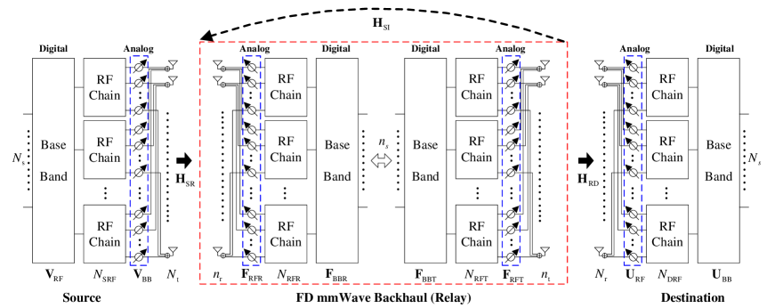
Figure 1: FD mmWave relay systems with hybrid analog and digital structure

$${\bf y}_{\text{R}}={\bf H}_{\text{SR}}{\bf x}_{\text{S}}+{\bf H}_{\text{SI}}{\bf x}_{\text{R}}+{\bf n}_{\text{R}},$$ (2)

where ${\bf H}_{\text{SR}}\in\mathbb{C}^{n_{\text{r}}\times N_{\text{t}}}$ denotes the source-to-relay channel matrix, ${\bf H}_{\text{SI}}\in\mathbb{C}^{n_{\text{r}}\times n_{\text{t}}}$ denotes the SI channel of relay, ${\bf x}_{\text{R}}\in\mathbb{C}^{n_{\text{t}}\times 1}$ denotes the transmitted signal at the relay, and ${\bf n}_{\text{R}}\sim\mathcal{CN}(0,\sigma_{\text{n}}^{2}{\bf I}_{n_{\text{R}}})$ denotes the noise vector at the relay. At the relay, the received signal ${\bf y}_{\text{R}}$ is firstly combined with the analog precoding matrix ${\bf F}_{\text{RFR}}\in\mathbb{C}^{n_{\text{r}}\times N_{\text{RFR}}}$ and digital precoding matrix ${\bf F}_{\text{BBR}}\in\mathbb{C}^{N_{\text{RFR}}\times n_{\text{s}}}$. Then, it is precoded by digital precoding matrix ${\bf F}_{\text{BBT}}\in\mathbb{C}^{N_{\text{RFT}}\times n_{\text{s}}}$ and analog precoding matrix ${\bf F}_{\text{RFT}}\in\mathbb{C}^{n_{\text{t}}\times N_{\text{RFT}}}$. Thus, the transmitted signal at the relay is expressed as

$${\bf x}_{\text{R}}=\sqrt{P_{\text{R}}}{\bf F}_{\text{RFT}}{\bf F}_{\text{BBT}}{\bf F}_{\text{BBR}}^{H}{\bf F}_{\text{RFR}}^{H}{\bf y}_{\text{R}},$$ (3)

where ${P_{\text{R}}}$ is the transmit power of the relay. Plugging (1) and (2) into (3), we obtain

$${\bf x}_{\text{R}}）= {\bf F}_{\text{RFT}}{\bf F}_{\text{BBT}}\left({\bf I}_{n_{\text{s}}}-\sqrt{P_{\text{R}}}{\bf F}_{\text{BBR}}^{H}{\bf F}_{\text{RFR}}^{H}{\bf H}_{\text{SI}}{\bf F}_{\text{RFT}}{\bf F}_{\text{BBT}}\right)^{-1}$$ (4)

$$\times\sqrt{P_{\text{R}}}{\bf F}_{\text{BBR}}^{H}{\bf F}_{\text{RFR}}^{H}\left(\sqrt{P_{\text{S}}}{\bf H}_{\text{SR}}{\bf V}_{\text{RF}}{\bf V}_{\text{BB}}{\bf{s}}_{\text{S}}+{\bf n}_{\text{R}}\right).$$

At the destination, the received signal is multiplied by the analog combining matrix ${\bf U}_{\text{RF}}\in\mathbb{C}^{N_{\text{r}}\times N_{\text{RFD}}}$ and digital combining matrix ${\bf U}_{\text{BB}}\in\mathbb{C}^{N_{\text{RFD}}\times N_{\text{s}}}$, which is expressed as

$$\begin{split}{\bf y}_{\text{D}}）=&\sqrt{P_{\text{S}}P_{\text{R}}}{\bf U}^{H}{\bf H}_{\text{RD}}{\bf F}_{\text{T}}{\bf\Xi}_{\text{R}}^{-1}{\bf F}_{\text{R}}^{H}{\bf H}_{\text{SR}}{\bf V}{\bf{s}}_{\text{S}}\\ &+\sqrt{P_{\text{R}}}{\bf U}^{H}{\bf H}_{\text{RD}}{\bf F}_{\text{T}}{\bf\Xi}_{\text{R}}^{-1}{\bf F}_{\text{R}}^{H}{\bf n}_{\text{R}}+{\bf U}^{H}{\bf n}_{\text{D}},\end{split}$$ (5)

where ${\bf V}={\bf V}_{\text{RF}}{\bf V}_{\text{BB}}$, ${\bf U}={\bf U}_{\text{RF}}{\bf U}_{\text{BB}}$, ${\bf F}_{\text{T}}={\bf F}_{\text{RFT}}{\bf F}_{\text{BBT}}$, ${\bf F}_{\text{R}}={\bf F}_{\text{RFR}}{\bf F}_{\text{BBR}}$, and ${\bf\Xi}_{\text{R}}={\bf I}_{n_{\text{s}}}-\sqrt{P_{\text{R}}}{\bf F}_{\text{R}}^{H}{\bf H}_{\text{SI}}{\bf F}_{\text{T}}$. ${\bf H}_{\text{RD}}\in\mathbb{C}^{N_{\text{r}}\times n_{\text{t}}}$ denotes the relay-to-destination channel matrix and ${\bf n}_{\text{D}}\sim\mathcal{CN}(0,\sigma_{\text{n}}^{2}{\bf I}_{N_{\text{r}}})$ denotes the noise vector at destination.

From the above, the spectral efficiency of the system is given by

$$\begin{split}R=&\log_{2}\left|{\bf I}_{N_{\text{s}}}+\frac{P_{\text{S}}P_{\text{R}}}{N_{\text{s}}}{\bf\Sigma}^{-1}\left({\bf U}^{H}{\bf H}_{\text{RD}}{\bf F}_{\text{T}}{\bf\Xi}_{\text{R}}^{-1}{\bf F}_{\text{R}}^{H}{\bf H}_{\text{SR}}{\bf V}\right)\right.\\ &\left.\times\left({\bf U}^{H}{\bf H}_{\text{RD}}{\bf F}_{\text{T}}{\bf\Xi}_{\text{R}}^{-1}{\bf F}_{\text{R}}^{H}{\bf H}_{\text{SR}}{\bf V}\right)^{H}\right|,\end{split}$$ (6)

where ${\bf\Sigma}=\sigma_{\text{n}}^{2}\big{[}{P_{\text{R}}}\left({\bf U}^{H}{\bf H}_{\text{RD}}{\bf F}_{\text{T}}{\bf\Xi}_{\text{R}}^{-1}{\bf F}_{\text{R}}^{H}\right)\left({\bf U}^{H}{\bf H}_{\text{RD}}{\bf F}_{\text{T}}{\bf\Xi}_{\text{R}}^{-1}{\bf F}_{\text{R}}^{H}\right)^{H}+{\bf U}^{H}{\bf U}\big{]}$ is the covariance matrix of the noise term in (5).

II-B Channel model

For the desired link channels (i.e., ${\bf H}_{\text{SR}}$ and ${\bf H}_{\text{RD}}$), we assume that sufficient far-field conditions have been met, and employ the extended Saleh-Valenzuela mmWave channel model [1, 2] to characterize the limited scattering features of mmWave channels. This model is described as the sum of the contributions from $N_{\text{c}}$ scattering clusters, each of which contributes $N_{\text{p}}$ propagation paths. This model expresses the mmWave channel as

$${\bf H}=\sqrt{\frac{N_{\text{R}}N_{\text{T}}}{N_{\text{c}}N_{\text{p}}}}\sum_{k=1}^{N_{\text{c}}}\sum_{l=1}^{N_{\text{p}}}\alpha_{k,l}{\bf{a}}(\theta_{k,l}^{\text{r}}){\bf{a}}(\theta_{k,l}^{\text{t}})^{H},$$ (7)

where $N_{\text{T}}$ denotes the number of transmit antennas, $N_{\text{R}}$ denotes the number of receive antennas, $\alpha_{k,l}$ denotes the complex gain of the $l$-th ray in the $k$-th propagation cluster. The functions ${\bf{a}}(\theta_{k,l}^{\text{r}})$ and ${\bf{a}}(\theta_{k,l}^{\text{t}})^{H}$ respectively represent the normalized receive and transmit array response vectors, where $\theta_{k,l}^{\text{r}}$ and $\theta_{k,l}^{\text{t}}$ are the azimuth angles of arrival and departure, respectively. The array response can be expressed as

$${\bf{a}}(\theta)=\frac{1}{{\sqrt{{N}}}}{\left[1,{e^{-j\frac{{2\pi d}}{\lambda}\sin(\theta)}},...,{e^{-j({N}-1)\frac{{2\pi d}}{\lambda}\sin(\theta)}}\right]^{T}},$$ (8)

where $d$ is the antenna spacing and $\lambda$ is the carrier wave-length.

$$d_{m,n}=\sqrt{(a_{0}+(m-1)d)^{2}+(b_{0}+(n-1)d)^{2}-2(a_{0}+(m-1)d)(b_{0}+(n-1)d)\cos(\phi)},$$ (10)

$$\begin{split}\mathop{\max}\limits_{\scriptstyle{\bf V}_{\text{RF}},{\bf U}_{\text{RF}},{\bf F}_{\text{RFT}},{\bf F}_{\text{RFR}}\hfill\atop\scriptstyle{\bf V}_{\text{BB}},{\bf U}_{\text{BB}},{\bf F}_{\text{BBT}},{\bf F}_{\text{BBR}}\hfill}&R=\log_{2}\left|{\bf I}_{N_{\text{s}}}+\frac{P_{\text{S}}P_{\text{R}}}{N_{\text{s}}}\Sigma^{-1}\left[{\bf U}^{H}{\bf H}_{\text{RD}}{\bf F}_{\text{T}}{\bf F}_{\text{R}}^{H}{\bf H}_{\text{SR}}{\bf V}\right]\left[{\bf U}^{H}{\bf H}_{\text{RD}}{\bf F}_{\text{T}}{\bf F}_{\text{R}}^{H}{\bf H}_{\text{SR}}{\bf V}\right]^{H}\right|\\ \text{s.t.}\qquad~{}~{}&{\bf V}_{\text{RF}}\in\mathcal{W}_{\text{RF}},{\bf U}_{\text{RF}}\in\mathcal{G}_{\text{RF}},{\bf F}_{\text{RFR}}\in\mathcal{F}_{\text{RFR}},{\bf F}_{\text{RFT}}\in\mathcal{F}_{\text{RFT}},\\ &\left\|{\bf F}_{\text{RFT}}{\bf F}_{\text{BBT}}\right\|_{\text{F}}^{2}=N_{\text{s}},\\ &\left\|{\bf V}_{\text{RF}}{\bf V}_{\text{BB}}\right\|_{\text{F}}^{2}=N_{\text{s}},\\ &{\bf F}_{\text{R}}^{H}{\bf H}_{\text{SI}}{\bf F}_{\text{T}}=0,\end{split}$$ (12)

Based on the widely used mmWave SI channel in [2, 7, 10], the residual SI consists of two parts: LOS SI and NLOS SI. With the high beam gain of mmWave signals, the NLOS SI results from refection from nearby obstacles. We can utilize the far-filed clustered mmWave channel in (7) to model the NLOS SI channel. By contrast, in the FD scenario, since the transmitter and the local receiver are closely placed, LOS SI channels are near-field channels and clustered mmWave channels cannot be used. Therefore, a more realistic SI channel model, which is the spherical wave propagation model, is considered for the near-field LOS channel matrix. According to [2, 10], the LOS SI channel coefficient of the $m$-th row and $n$-th column entry is given by

$$\left[{\bf H}_{\text{LOS}}\right]_{m,n}=\frac{\rho}{d_{m,n}}\exp\left(-j\frac{2\pi}{\lambda}d_{m,n}\right),$$ (9)

where $\rho$ is a normalization constant such that $\mathbb{E}[\left\|{\bf H}_{\text{LOS}}\right\|_{\text{F}}^{2}]=n_{\text{t}}n_{\text{r}}$ and $d_{m,n}$ is the distance from the $m$-th element of the transmit array to the $n$-th element of the receive array, expressed in (10), with $\phi$ corresponding to the angle between the two antenna arrays, and $a_{0}$ and $b_{0}$ denoting the initial distances of the antennas to a common reference point. Finally, the FD mmWave SI channel is constructed as

$${\bf H}_{\text{SI}}=\kappa_{\text{LOS}}{\bf H}_{\text{LOS}}+\kappa_{\text{NLOS}}{\bf H}_{\text{NLOS}},$$ (11)

where $\kappa_{\text{LOS}}$ and $\kappa_{\text{NLOS}}$ denote the intensity coefficients of LOS and NLOS components, respectively.

II-C Problem formulation

The main objective of this work is to maximize the system spectral efficiency by jointly designing beamforming matrices (i.e., ${\bf V}_{\text{RF}}$, ${\bf V}_{\text{BB}}$, ${\bf F}_{\text{RFT}}$, ${\bf F}_{\text{BBT}}$, ${\bf F}_{\text{RFR}}$, ${\bf F}_{\text{BBR}}$, ${\bf U}_{\text{RF}}$ and ${\bf U}_{\text{BB}}$) and SIC in the presence of noisy CSI. The HBF design problem of maximizing the system spectral efficiency is given by (12), where $\mathcal{V}_{\text{RF}}$, $\mathcal{U}_{\text{RF}}$, $\mathcal{F}_{\text{RFR}}$ and $\mathcal{F}_{\text{RFT}}$ are the feasible sets of the analog precoders included by unit modulus constraints. Due to the non-convex constraints of the analog precoders and ${\bf F}_{\text{R}}^{H}{\bf H}_{\text{SI}}{\bf F}_{\text{T}}=0$, it is in general intractable to solve the optimization problem. Meanwhile, the HBF design with conventional optimization-based approaches are not robust in the presence of noisy CSI. To solve these problems, we first develop algorithms that maximize the spectral efficiency with joint HBF and SIC design. Then, learning machines (e.g., ELM and CNN) are adopted such that the hybrid beamformers are predicted by feeding the machines with noisy CSI.

III FD mmWave beamforming design

In order to train the ELM and CNN learning machines, we first need to solve the optimization problem in (12) to provide accurate labels of the training data samples. Generally, to make the problem tractable and reduce the communication overhead, the beamformers can be designed individually at different nodes [2, 7]. The main challenge is at the relay node since the beamformers of the transmitting part and receiving part should be jointly designed, and SIC needs to be guaranteed. Consequently, we first propose efficient algorithms to design the hybrid beamformers at the relay, and then HBF design at the source and destination can be obtained following similar approaches at relay.

III-A SIC and HBF algorithm design

According to the method studied in [4, 25, 26], the HBF design problem at the relay can be transferred into minimizing the Frobenius norm of the difference between the optimal fully digital beamformer and hybrid beamformers as

$$\begin{split}(\text{P}1):~{}\mathop{\min}\limits_{{\bf F}_{\text{RFT}},{\bf F}_{\text{BBT}},{\bf F}_{\text{RFR}},{\bf F}_{\text{BBR}}}&\left\|{\bf F}_{\text{opt}}-{\bf F}_{\text{RFT}}{\bf F}_{\text{BBT}}{\bf F}_{\text{BBR}}^{H}{\bf F}_{\text{RFR}}^{H}\right\|_{\text{F}}^{2}\\ \text{s.t.}~{}~{}\qquad&{\bf F}_{\text{RFR}}\in\mathcal{F}_{\text{RFR}},{\bf F}_{\text{RFT}}\in\mathcal{F}_{\text{RFT}},\\ &\left\|{\bf F}_{\text{RFT}}{\bf F}_{\text{BBT}}\right\|_{\text{F}}^{2}=n_{\text{s}},\\ &{\bf F}_{\text{BBR}}^{H}{\bf F}_{\text{RFR}}^{H}{\bf H}_{\text{SI}}{\bf F}_{\text{RFT}}{\bf F}_{\text{BBT}}=0,\end{split}$$ (13)

where ${\bf F}_{\text{opt}}={\bf F}_{\text{TSVD}}{\bf F}_{\text{RSVD}}^{H}$, ${\bf F}_{\text{TSVD}}$ and ${\bf F}_{\text{RSVD}}$ are formed by the right-singular vectors of ${\bf H}_{\text{RD}}$ and left-singular vectors of ${\bf H}_{\text{SR}}$, respectively.

Due to the non-convex constraints, it is still hard to find a solution of problem (P1) that guarantees both SIC and optimal hybrid beamformers. Moreover, according to the results in [2, 7], the spectral efficiency of FD mmWave systems degrades significantly if residual SI cannot be efficiently suppressed. Thus, we will solve this problem following two steps. In the first step, we mainly focus on perfectly eliminating SI (i.e., ${\bf F}_{\text{BBR}}^{H}{\bf F}_{\text{RFR}}^{H}{\bf H}_{\text{SI}}{\bf F}_{\text{RFT}}{\bf F}_{\text{BBT}}=0$) by designing unconstrained beamformers for both transmitting and receiving parts. Then, the problem (P1) can be rewritten as

$$\begin{split}(\text{P}2):~{}\mathop{\min}\limits_{{\bf F}_{\text{T}},{\bf F}_{\text{R}}}~{}&\left\|{\bf F}_{\text{opt}}-{\bf F}_{\text{T}}{\bf F}_{\text{R}}^{H}\right\|_{\text{F}}^{2}\\ \quad\text{s.t.}~{}~{}&{\bf F}_{\text{R}}^{H}{\bf H}_{\text{SI}}{\bf F}_{\text{T}}=0.\\ \end{split}$$ (14)

After solving (P2), we obtain the unconstrained beamformers that can ensure perfect SIC. In the second step, hybrid beamformers of the transmitting part and receiving part are jointly designed by minimizing the Frobenius norm of the difference between the unconstrained beamformers and hybrid beamformers. The problem is formulated as

$$\begin{split}(\text{P}3):~{}\mathop{\min}\limits_{{\bf F}_{\text{RFT}},{\bf F}_{\text{BBT}},{\bf F}_{\text{RFR}},{\bf F}_{\text{BBR}}}~{}&\left\|\hat{\bf F}_{\text{opt}}-{\bf F}_{\text{RFT}}{\bf F}_{\text{BBT}}{\bf F}_{\text{BBR}}^{H}{\bf F}_{\text{RFR}}^{H}\right\|_{\text{F}}^{2}\\ \qquad\text{s.t.}~{}~{}~{}~{}\quad\quad&{\bf F}_{\text{RFR}}\in\mathcal{F}_{\text{RFR}},{\bf F}_{\text{RFT}}\in\mathcal{F}_{\text{RFT}},\\ \qquad\quad\qquad&\left\|{\bf F}_{\text{RFT}}{\bf F}_{\text{BBT}}\right\|_{\text{F}}^{2}=n_{\text{s}},\\ \end{split}$$ (15)

where $\hat{\bf F}_{\text{opt}}=\hat{\bf F}_{\text{T}}\hat{\bf F}_{\text{R}}^{H}$ with $\hat{\bf F}_{\text{T}}$ and $\hat{\bf F}_{\text{R}}$ corresponding to the solutions of problem (P2). Though problems (P2) and (P3) are simpler than the original problem (P1), both problems are still non-convex problems and efficient approaches should be proposed to solve them.

Let us start with problem (P2). It is obvious that this problem is convex when one of the variables is fixed. This property enables ADMM utilization, and consequently, the augmented Lagrangian function of (P2) is given by

$$\mathcal{L}({\bf F}_{\text{T}},{\bf F}_{\text{R}},{\bf Z})=\left\|{\bf F}_{\text{opt}}-{\bf F}_{\text{T}}{\bf F}_{\text{R}}^{H}\right\|_{\text{F}}^{2}+\varrho\left\|{\bf F}_{\text{R}}^{H}{\bf H}_{\text{SI}}{\bf F}_{\text{T}}+\frac{1}{\varrho}{\bf Z}\right\|_{\text{F}}^{2},$$ (16)

where ${\bf Z}\in\mathbb{C}^{n_{\text{s}}\times n_{\text{s}}}$ is the Lagrange multiplier matrix and $\varrho$ is the ADMM step-size. According to ADMM approaches[27], the solution to (P2) can be obtained iteratively, where in iteration $i+1$, the variables and multiplier are updated as follows

$${\bf F}_{\text{T}}^{(i+1)}:= \arg\mathop{\min}\limits_{{\bf F}_{\text{T}}}\mathcal{L}\left({\bf F}_{\text{T}},{\bf F}_{\text{R}}^{(i)},{\bf Z}^{(i)}\right);$$ (17a)

$${\bf F}_{\text{R}}^{(i+1)}:= \arg\mathop{\min}\limits_{{\bf F}_{\text{R}}}\mathcal{L}\left({\bf F}_{\text{T}}^{(i+1)},{\bf F}_{\text{R}},{\bf Z}^{(i)}\right);$$ (17b)

$${\bf Z}^{(i+1)}:= {\bf Z}^{(i)}+\varrho{\bf F}_{\text{R}}^{H{(i+1)}}{\bf H}_{\text{SI}}{\bf F}_{\text{T}}^{(i+1)}.$$ (17c)

By solving the problems in (17a) and (17b), we have the following theorem.

Theorem 1.

The closed-form expressions for ${\bf F}_{\rm{T}}^{(i+1)}$ and ${\bf F}_{\rm{R}}^{(i+1)}$ are receptively given by

$$\begin{split}\text{vec}\left({\bf F}_{\rm{T}}^{(i+1)}\right)=&\left[{\bf I}_{n_{\rm{s}}}\otimes\left(\varrho{\bf H}_{\rm{SI}}^{H}{\bf F}_{\rm{R}}^{(i)}{\bf F}_{\rm{R}}^{H(i)}{\bf H}_{\rm{SI}}\right)+\left({\bf F}_{\rm{R}}^{H(i)}{\bf F}_{\rm{R}}^{(i)}\right)\otimes{\bf I}_{n_{\rm{t}}}\right]^{-1}\\ &\times\text{vec}\left({\bf F}_{\rm{opt}}{\bf F}_{\rm{R}}^{(i)}-{\bf H}_{\rm{SI}}^{H}{\bf F}_{\rm{R}}^{(i)}{\bf Z}^{(i)}\right),\\ \end{split}$$ (18)

and

$$\begin{split}&\text{vec}\left({\bf F}_{\rm{R}}^{(i+1)}\right)\\ &=\left[\left(\varrho{\bf H}_{\rm{SI}}{\bf F}_{\rm{T}}^{(i+1)}{\bf F}_{\rm{T}}^{H(i+1)}{\bf H}_{\rm{SI}}^{H}\right)\otimes{\bf I}_{n_{\rm{s}}}+{\bf I}_{n_{\rm{r}}}\otimes\left({\bf F}_{\rm{T}}^{H(i+1)}{\bf F}_{\rm{T}}^{(i+1)}\right)\right]^{-1}\\ &~{}~{}~{}\times\text{vec}\left({\bf F}_{\rm{T}}^{H(i+1)}{\bf F}_{\rm{opt}}-{\bf Z}^{(i)}{\bf F}_{\rm{T}}^{H(i+1)}{\bf H}_{\rm{SI}}^{H}\right).\\ \end{split}$$ (19)

Proof.

We first solve problem (17a). By taking the derivative of $\mathcal{L}\big{(}{\bf F}_{\text{T}},{\bf F}_{\text{R}}^{(i)},{\bf Z}^{(i)}\big{)}$ over ${\bf F}_{\text{T}}$ and letting it to be zero, we have ${\bf F}_{\text{T}}{\bf F}_{\text{R}}^{H(i)}{\bf F}_{\text{R}}^{(i)}+\varrho{\bf H}_{\text{SI}}^{H}{\bf F}_{\text{R}}^{(i)}{\bf F}_{\text{R}}^{H(i)}{\bf H}_{\text{SI}}{\bf F}_{\text{T}}={\bf F}_{\text{opt}}{\bf F}_{\text{R}}^{(i)}-{\bf H}_{\text{SI}}^{H}{\bf F}_{\text{R}}^{(i)}{\bf Z}^{(i)}$. Then, utilizing the vectorization property, the result in (18) can be obtained. For the problem (17b), we can use a similar approach of the problem (17a) and obtain ${\bf F}_{\text{R}}^{(i+1)}$ in (19). ∎

The above alternating procedure is initialized by setting the entries of matrices ${\bf F}_{\text{R}}^{(0)}$ to random values, and multiplier ${\bf Z}^{(0)}$ to zeros. After obtaining the updated variables in each steps, we summarize the ADMM-based beamforming design and SIC approach in Algorithm 1.

1:  Input: ${\bf F}_{\text{opt}}$, ${\bf H}_{\text{SI}}$, $\varrho$;

2:  Output: ${\bf F}_{\text{T}}$, ${\bf F}_{\text{R}}$;

3:  Initialize: ${\bf F}_{\text{R}}^{(0)}$, ${\bf Z}^{(0)}$ and $i=0$;

4:  repeat

5:     Update ${\bf F}_{\text{T}}^{(i+1)}$ using (18);

6:     Update ${\bf F}_{\text{R}}^{(i+1)}$ using (19);

7:     Update ${\bf Z}^{(i+1)}$ using (17c);

8:     $i\leftarrow i+1$;

9:  until the stopping criteria is met.

Algorithm 1 ADMM-based beamforming and SI cancellation algorithm

After obtaining the solutions of problem (P2), we then turn to solve problem (P3). The main challenges for this problem are the constant modulus non-convex constraints and the joint optimization of transmitting and receiving hybrid beamformers. Furthermore, since the beamformers derived by Algorithm 1 for SIC may not be mutually orthogonal, many existing approaches (e.g., PE-AltMin [22], GEVD [23] and methods in [24]) cannot be directly used for this case. To make this problem tractable and deal with the non-convex constraints, we utilize majorization-minimization (MM) methods [28, 29, 30]. In stead of minimizing the original objective function directly, the MM procedure consists of two steps. In the first majorization step, we find an easy implemented surrogate function that should be a tight upper bound of the original objective function and exist closed-from minimizers. Then in the minimization step, we minimize the surrogate function with closed-from minimizers. To achieve a fast convergence rate, a surrogate function that tries to follow the shape of the objective function is preferable[28].

To jointly design the hybrid beamformers at transmitting and receiving parts with MM methods, we will solve problem (P3) based on the alternating minimization framework. We first solve problem (P3) for the transmitting precoder ${\bf F}_{\text{RFT}}$ by fixing ${\bf F}_{\text{RFR}}$, ${\bf F}_{\text{BBR}}$ and ${\bf F}_{\text{BBT}}$. Problem (P3) can be rewritten as

$$\begin{split}(\text{P}4):~{}&\mathop{\min}\limits_{{\bf F}_{\text{RFT}}}~{}\left\|\hat{\bf F}_{\text{opt}}-{\bf F}_{\text{RFT}}{\bf Y}_{\text{T}}\right\|_{\text{F}}^{2}\\ &~{}\text{s.t.}~{}~{}~{}~{}{\bf F}_{\text{RFT}}\in\mathcal{F}_{\text{RFT}},\\ \end{split}$$ (20)

where ${\bf Y}_{\text{T}}={\bf F}_{\text{BBT}}{\bf F}_{\text{BBR}}^{H}{\bf F}_{\text{RFR}}^{H}$. Then, we rewrite the objective function of problem (P4) as

$$\begin{split}J({\bf F}_{\text{RFT}};{\bf Y}_{\text{T}})&=\text{Tr}\left(\hat{\bf F}_{\text{opt}}\hat{\bf F}_{\text{opt}}^{H}\right)+\text{Tr}\left({\bf F}_{\text{RFT}}^{H}{\bf F}_{\text{RFT}}{\bf Y}_{\text{T}}{\bf Y}_{\text{T}}^{H}\right)\\ &\quad-\text{Tr}\left(\hat{\bf F}_{\text{opt}}{\bf Y}_{\text{T}}^{H}{\bf F}_{\text{RFT}}^{H}\right)-\text{Tr}\left({\bf F}_{\text{RFT}}\left(\hat{\bf F}_{\text{opt}}{\bf Y}_{\text{T}}^{H}\right)^{H}\right)\\ &\mathop{=}\limits^{(a)}\text{Tr}\left(\hat{\bf F}_{\text{opt}}\hat{\bf F}_{\text{opt}}^{H}\right)+{\bf f}_{\text{RFT}}^{H}{\bf Q}_{\text{T}}{\bf f}_{\text{RFT}}-2\text{Re}\left({\bf f}_{\text{RFT}}^{H}{\bf e}_{\text{T}}\right),\end{split}$$ (21)

where ${\bf f}_{\text{RFT}}=\text{vec}({\bf F}_{\text{RFT}})$, ${\bf E}_{\text{T}}=\hat{\bf F}_{\text{opt}}{\bf Y}_{\text{T}}^{H}$, ${\bf e}_{\text{T}}=\text{vec}({\bf E}_{\text{T}})$, ${\bf Q}_{\text{T}}=({\bf Y}_{\text{T}}{\bf Y}_{\text{T}}^{H})^{T}\otimes{\bf I}_{n_{\text{t}}}$, and (a) follows from the identity $\text{Tr}({\bf A}{\bf B}{\bf C}{\bf D})=\text{vec}({\bf A}^{T})^{T}({\bf D}^{T}\otimes{\bf B})\text{vec}({\bf C})$.

To solve problem (P4) with MM methods, we should find a majorizer of $J({\bf F}_{\text{RFT}};{\bf Y}_{\text{T}})$ according to the following lemma.

Lemma 1.

Let ${\bf Q}\in\mathbb{C}^{N\times N}$ and ${\bf S}\in\mathbb{C}^{N\times N}$ be two Hermitian matrices satisfying ${\bf S}\geq{\bf Q}$. Then the quadratic function ${\bf a}^{H}{\bf Q}{\bf a}$, is majorized by ${\bf a}^{H}{\bf S}{\bf a}+2\text{Re}({\bf a}^{H}({\bf Q}-{\bf S}){\bf a}_{i})+{\bf a}_{i}^{H}({\bf S}-{\bf Q}){\bf a}_{i}$ at point ${\bf a}_{i}\in\mathbb{C}^{N}$.

Proof.

The proof can be found in [29]. ∎

According to Lemma 1, we can obtain a valid majorizer of $J({\bf F}_{\text{RFT}};{\bf Y}_{\text{T}})$ at point ${\bf F}_{\text{RFT}}^{(i)}\in\mathcal{F}_{\text{RFT}}$ given by

$$\begin{split}&\bar{J}\left({\bf F}_{\text{RFT}};{\bf Y}_{\text{T}},{\bf F}_{\text{RFT}}^{(i)}\right)\\ =&\text{Tr}\left(\hat{\bf F}_{\text{opt}}\hat{\bf F}_{\text{opt}}^{H}\right)+\lambda_{\text{T}}{\bf f}_{\text{RFT}}^{H}{\bf f}_{\text{RFT}}+2\text{Re}\left({\bf f}_{\text{RFT}}^{H}\left({\bf Q}_{\text{T}}-\lambda_{\text{T}}{\bf I}\right){\bf f}_{\text{RFT}}^{(i)}\right)\\ &+{\bf f}_{\text{RFT}}^{H(i)}\left(\lambda_{\text{T}}{\bf I}-{\bf Q}_{\text{T}}\right){\bf f}_{\text{RFT}}^{(i)}-2\text{Re}\left({\bf f}_{\text{RFT}}^{H}{\bf e}_{\text{T}}\right)\\ =&2\text{Re}\left({\bf f}_{\text{RFT}}^{H}\left(\left({\bf Q}_{\text{T}}-\lambda_{\text{T}}{\bf I}\right){\bf f}_{\text{RFT}}^{(i)}-{\bf e}_{\text{T}}\right)\right)+C_{\text{T}},\end{split}$$ (22)

where ${\bf F}_{\text{RFT}}^{(i)}$ is the iterate available at $i$-th iteration, $\lambda_{\text{T}}$ denotes the maximum eigenvalue of ${\bf Q}_{\text{T}}$, and the constant term $C_{\text{T}}=\text{Tr}(\hat{\bf F}_{\text{opt}}\hat{\bf F}_{\text{opt}}^{H})+\lambda_{\text{T}}{\bf f}_{\text{RFT}}^{H}{\bf f}_{\text{RFT}}+{\bf f}_{\text{RFT}}^{H(i)}(\lambda_{\text{T}}{\bf I}-{\bf Q}_{\text{T}}){\bf f}_{\text{RFT}}^{(i)}$. Thus, we can guarantee $\lambda_{\text{T}}{\bf I}\geq{\bf Q}_{\text{T}}$. Then, utilizing the majorizer in (22), the solution of problem (P4) can be obtained by iteratively solving the following problem

$$\begin{split}(\text{P}5):~{}&{\bf F}_{\text{RFT}}^{(i+1)}=\arg\mathop{\min}\limits_{{\bf F}_{\text{RFT}}}~{}\bar{J}\left({\bf F}_{\text{RFT}};{\bf Y}_{\text{T}},{\bf F}_{\text{RFT}}^{(i)}\right)\\ &~{}~{}\text{s.t.}~{}~{}~{}{\bf F}_{\text{RFT}}\in\mathcal{F}_{\text{RFT}}.\\ \end{split}$$ (23)

The close-form solution of problem (P5) is given by

$${\bf f}_{\text{RFT}}^{(i+1)}=-\exp\left(j\arg\left(\left({\bf Q}_{\text{T}}-\lambda_{\text{T}}{\bf I}\right){\bf f}_{\text{RFT}}^{(i)}-{\bf e}_{\text{T}}\right)\right).$$ (24)

Similarly, we can solve problem (P3) for the receiving combiner ${\bf F}_{\text{RFR}}$ by fixing ${\bf F}_{\text{RFT}}$, ${\bf F}_{\text{BBR}}$ and ${\bf F}_{\text{BBT}}$. Then, problem (P3) can be rewritten as

$$\begin{split}(\text{P}6):~{}&\mathop{\min}\limits_{{\bf F}_{\text{RFR}}}~{}\text{Tr}\left(\hat{\bf F}_{\text{opt}}\hat{\bf F}_{\text{opt}}^{H}\right)+{\bf f}_{\text{RFR}}^{H}{\bf Q}_{\text{R}}{\bf f}_{\text{RFR}}-2\text{Re}\left({\bf f}_{\text{RFR}}^{H}{\bf e}_{\text{R}}\right)\\ &~{}~{}\text{s.t.}~{}~{}~{}{\bf F}_{\text{RFR}}\in\mathcal{F}_{\text{RFR}},\\ \end{split}$$ (25)

where ${\bf Q}_{\text{R}}=({\bf Y}_{\text{R}}^{H}{\bf Y}_{\text{R}})^{T}\otimes{\bf I}_{n_{\text{r}}}$, ${\bf Y}_{\text{R}}={\bf F}_{\text{RFT}}{\bf F}_{\text{BBT}}{\bf F}_{\text{BBR}}^{H}$, ${\bf f}_{\text{RFR}}=\text{vec}({\bf F}_{\text{RFR}})$, ${\bf E}_{\text{R}}=\hat{\bf F}_{\text{opt}}^{H}{\bf Y}_{\text{R}}$, and ${\bf e}_{\text{R}}=\text{vec}({\bf E}_{\text{R}})$. According to Lemma 1, we can obtain a valid majorizer of the objective function in (25) at point ${\bf F}_{\text{RFR}}^{(i)}\in\mathcal{F}_{\text{RFR}}$, which is given by

$$\begin{split}\tilde{J}\left({\bf F}_{\text{RFR}};{\bf Y}_{\text{R}},{\bf F}_{\text{RFR}}^{(i)}\right)=2\text{Re}\left({\bf f}_{\text{RFR}}^{H}\left(\left({\bf Q}_{\text{R}}-\lambda_{\text{R}}{\bf I}\right){\bf f}_{\text{RFR}}^{(i)}-{\bf e}_{\text{R}}\right)\right)+C_{\text{R}},\end{split}$$ (26)

where $\lambda_{\text{R}}$ denotes the maximum eigenvalue of ${\bf Q}_{\text{R}}$ and the constant term $C_{\text{R}}=\text{Tr}(\hat{\bf F}_{\text{opt}}\hat{\bf F}_{\text{opt}}^{H})+\lambda_{\text{R}}{\bf f}_{\text{RFR}}^{H}{\bf f}_{\text{RFR}}+{\bf f}_{\text{RFR}}^{H(i)}(\lambda_{\text{R}}{\bf I}-{\bf Q}_{\text{R}}){\bf f}_{\text{RFR}}^{(i)}$. Following a similar procedure of solving problem (P4), the solution of problem (P6) can be obtained by iteratively updating ${\bf F}_{\text{RFR}}$ according to the following close-form expression

$${\bf f}_{\text{RFR}}^{(i+1)}=-\exp\left(j\arg\left(\left({\bf Q}_{\text{R}}-\lambda_{\text{R}}{\bf I}\right){\bf f}_{\text{RFT}}^{(i)}-{\bf e}_{\text{R}}\right)\right).$$ (27)

Then, we turn to design digital beamformers (i.e., ${\bf F}_{\text{BBR}}$ and ${\bf F}_{\text{BBT}}$) with fixed analog beamformers (i.e., ${\bf F}_{\text{RFR}}$ and ${\bf F}_{\text{RFT}}$). By fixing ${\bf F}_{\text{BBT}}$, ${\bf F}_{\text{RFR}}$ and ${\bf F}_{\text{RFT}}$, a globally optimal solution of problem (P3) is given by

$${\bf F}_{\text{BBR}}={\bf F}_{\text{RFR}}^{-1}\hat{\bf F}_{\text{opt}}^{H}\left({\bf F}_{\text{BBT}}^{H}{\bf F}_{\text{RFT}}^{H}\right)^{-1}.$$ (28)

Similarly, by fixing ${\bf F}_{\text{BBR}}$, ${\bf F}_{\text{RFR}}$ and ${\bf F}_{\text{RFT}}$, a solution of problem (P3) without considering the power constraint in (15) is given by

$${\bf F}_{\text{BBT}}={\bf F}_{\text{RFT}}^{-1}\hat{\bf F}_{\text{opt}}\left({\bf F}_{\text{BBR}}^{H}{\bf F}_{\text{RFR}}^{H}\right)^{-1}.$$ (29)

Then, to satisfy the power constraint in problem (P3), we can normalize ${\bf F}_{\text{BBT}}$ by a factor of $\frac{\sqrt{n_{\text{s}}}}{\left\|{\bf F}_{\text{RFT}}{\bf F}_{\text{BBT}}\right\|_{\text{F}}}$[22, 2]. Letting $J({\bf F}_{\text{RFT}},{\bf F}_{\text{BBT}},{\bf F}_{\text{BBR}},{\bf F}_{\text{RFR}})$ denote the objective function of problem (P3), the effectiveness of the normalization step is shown in the following remark.

Remark 1.

If $J({\bf F}_{\rm{RFT}},{\bf F}_{\rm{BBT}},{\bf F}_{\rm{BBR}},{\bf F}_{\rm{RFR}})\leq\delta$ when ignoring the power constraint in (15), $J({\bf F}_{\rm{RFT}},\hat{\bf F}_{\rm{BBT}},{\bf F}_{\rm{BBR}},{\bf F}_{\rm{RFR}})\leq 4\delta$, where $\hat{\bf F}_{\rm{BBT}}=\frac{\sqrt{n_{\text{s}}}}{\left\|{\bf F}_{\text{RFT}}{\bf F}_{\text{BBT}}\right\|_{\text{F}}}{\bf F}_{\rm{BBT}}$.

Proof.

The proof of Remark 1 is omitted here since it is similar to that in [22]. ∎

In Remark 1, it demonstrates that after minimizing the objective function of (P3) to a sufficiently small value $\delta$ when ignoring the power constraint in (15), the normalization step will also guarantee a small value $4\delta$ for minimizing the objective function.

With above close-form solutions in (24), (27), (28) and (29), the MM based HBF design for both transmuting and receiving parts at relay is summarized in Algorithm 2.

1:  Input: $\hat{\bf F}_{\text{opt}}$;

2:  Output: ${\bf F}_{\text{RFT}}$, ${\bf F}_{\text{BBT}}$, ${\bf F}_{\text{RFR}}$, ${\bf F}_{\text{BBR}}$;

3:  Initialize: ${\bf F}_{\text{RFT}}^{(0)}$, ${\bf F}_{\text{RFR}}^{(0)}$, ${\bf F}_{\text{BBR}}^{(0)}$ and outer iteration $k_{\text{o}}=0$;

4:  repeat

5:     Fix ${\bf F}_{\text{RFT}}^{(k_{\text{o}})}$, ${\bf F}_{\text{RFR}}^{(k_{\text{o}})}$ and ${\bf F}_{\text{BBR}}^{(k_{\text{o}})}$, compute ${\bf F}_{\text{BBT}}^{(k_{\text{o}}+1)}$

according to (29);

6:     Use MM method to compute ${\bf F}_{\text{RFT}}^{(k_{\text{o}}+1)}$:

7:     Initialize: ${\bf F}_{\text{RFT}}^{(0)}={\bf F}_{\text{RFT}}^{(k_{\text{o}})}$, and inner iteration $k_{\text{i}}=0$;

8:     repeat

9:        Compute ${\bf F}_{\text{RFT}}^{(k_{\text{i}}+1)}$ according to (24);

10:        $k_{\text{i}}\leftarrow k_{\text{i}}+1$;

11:     until the stopping criteria is met.

12:     Update: ${\bf F}_{\text{RFT}}^{(k_{\text{o}}+1)}={\bf F}_{\text{RFT}}^{(k_{\text{i}})}$;

13:     Fix ${\bf F}_{\text{RFT}}^{(k_{\text{o}}+1)}$, ${\bf F}_{\text{BBT}}^{(k_{\text{o}}+1)}$ and ${\bf F}_{\text{RFR}}^{(k_{\text{o}})}$, compute ${\bf F}_{\text{BBR}}^{(k_{\text{o}}+1)}$ according to (28);

14:     Use MM method to compute ${\bf F}_{\text{RFR}}^{(k_{\text{o}}+1)}$:

15:     Initialize: ${\bf F}_{\text{RFR}}^{(0)}={\bf F}_{\text{RFR}}^{(k_{\text{o}})}$, and inner iteration $k_{\text{i}}=0$;

16:     repeat

17:        Compute ${\bf F}_{\text{RFR}}^{(k_{\text{i}}+1)}$ according to (27);

18:        $k_{\text{i}}\leftarrow k_{\text{i}}+1$;

19:     until the stopping criteria is met.

20:     Update: ${\bf F}_{\text{RFR}}^{(k_{\text{o}}+1)}={\bf F}_{\text{RFR}}^{(k_{\text{i}})}$;

21:     $k_{\text{o}}\leftarrow k_{\text{o}}+1$;

22:  until the stopping criteria is met.

23:  Compute ${\bf F}_{\text{BBT}}=\frac{\sqrt{n_{\text{s}}}}{\left\|{\bf F}_{\text{RFT}}{\bf F}_{\text{BBT}}\right\|_{\text{F}}}{\bf F}_{\text{BBT}}$.

Algorithm 2 MM-based HBF algorithm

III-B Convergence analysis and computational complexity

The general formulation for problem (P2) can be given as

$$\min_{\bm{x},\bm{y}}~{}F(\bm{x},\bm{y}),~{}~{}\text{s.t.}~{}G(\bm{x},\bm{y})=0,$$ (30)

where $F(\cdot,\cdot)$ is bi-convex and $G(\cdot,\cdot)$ is bi-affine. According to [27], ADMM can be applied to solve problem (30). The convergence of Algorithm 1 is under research and would not be analyzed in this paper. Instead, we will show the convergence of Algorithm 1 by simulation result in Section V-A. We then summarize the main complexity of Algorithm 1 in the following theorem.

Theorem 2.

If $N_{\text{t}}=N_{\text{r}}=n_{\text{t}}=n_{\text{r}}$, the main complexity of Algorithm 1 is $\mathcal{O}(2K_{\text{A}}(n_{\text{s}}^{3}+1)N_{\text{t}}^{3})$, where $K_{\text{A}}$ is the number of iterations.

Proof.

For Algorithm 1, the main complexity in each iteration includes two parts:

1) Derive ${\bf F}_{\text{opt}}$ based on the singular value decomposition of two channel matrices (i.e., ${\bf H}_{\text{SR}}$ and ${\bf H}_{\text{RD}}$). According to [31], the main complexity in this part is $\mathcal{O}(\max(N_{\text{t}},n_{\text{r}})\min(N_{\text{t}},n_{\text{r}})^{2}+\max(N_{\text{r}},n_{\text{t}})\min(N_{\text{r}},n_{\text{t}})^{2})$.

2) Compute ${\bf F}_{\text{T}}$ and ${\bf F}_{\text{R}}$ according to (18) and (19), respectively. The main complexity in this part comes from the inversion operations in (18) and (19), which is $\mathcal{O}(n_{\text{s}}^{3}(n_{\text{t}}^{3}+n_{\text{r}}^{3}))$.

Thus, the main complexity of Algorithm 1 is given by $\mathcal{O}(K_{\text{A}}(\max(N_{\text{t}},n_{\text{r}})\min(N_{\text{t}},n_{\text{r}})^{2}+\max(N_{\text{r}},n_{\text{t}})\min(N_{\text{r}},n_{\text{t}})^{2}+n_{\text{s}}^{3}(n_{\text{t}}^{3}+n_{\text{r}}^{3})))$. ∎

The convergence and main complexity of Algorithm 2 are summarized in the following theorem.

Theorem 3.

The convergence of Algorithm 2 is guaranteed. If $n_{\text{t}}=n_{\text{r}}$ and $n_{\text{s}}=N_{\text{RFT}}=N_{\text{RFR}}$, the main complexity of Algorithm 2 is $\mathcal{O}(2K_{\text{out}}(K_{\text{in}}n_{\text{t}}^{3}N_{\text{RFT}}^{3}+n_{\text{t}}N_{\text{RFT}}^{2}+n_{\text{t}}n_{\text{s}}^{2}))$, where $K_{\text{out}}$ and $K_{\text{in}}$ are the numbers of outer and inner iterations, respectively

Proof.

See Appendix A ∎

For the hybrid beamformers design at source and destination, we can also utilize MM methods and follow similar procedures in Algorithm 2, and details are omitted for space limitation. Above proposed HBF algorithms are iterative algorithms and suffer from high computational complexity as the number of antennas increases. Further, the proposed HBF algorithms and existing optimization based algorithms are linear mapping from the channel matrix and the hybrid beamformers which require a real-time computation and are not robust to noisy channel input data. Driven by following advantages of ML[17]: (1) low complexity when solving optimization-based problem and (2) capable to extrapolate new features form noisy and limited training data, we will propose two learning based approaches to address these problems in the following section.

IV learning based FD mmwave beamforming design

In this section, we will present our learning frameworks for HBF design. Firstly, we present the framework of ELM to design hybrid beamformers and the training data generation approach for robust HBF design. Then, we briefly introduce the HBF design based on CNN.

IV-A FD mmwave beamforming design with ELM

Feedforward Neural Network (FNN) is a powerful tool for regression and classification [32, 33, 34]. As a special FNN, the single layer feedforward network (SLFN) has also been investigated for low complexity [35]. In the SLFN, the weights of input nodes are optimized through the training procedure. Moreover, ELM is developed in [36, 37, 38], which consists of only one hidden layer. The weights of input nodes and bias for the hidden nodes are generated randomly. It is shown that ELM can achieve fast running speed with acceptable generalization performance. Since the processing time is one of the bottleneck for low latency communication, using ELM for HBF design can significantly reduce the overall delay. Moreover, due to the hardware constraint (e.g., limited computational capability and memory resources) of mobile terminals, it is easy to implement ELM based component because of its simple architecture.

Thus, in what follows, we will utilize ELM to extract the features of FD mmWave channels and predict the hybrid beamformers for all nodes. As mentioned in Sec. III, we will design different ELM networks for different nodes. We mainly focus on the ELM network design for HBF of relay, since the ELM network designs for source and destination are straightforward following a similar approach to that of relay node.

We assume that the training dataset is $\mathcal{D}=\left\{(\bm{x}_{j},\bm{t}_{j})|j=1,\ldots,N\right\}$, where $\bm{x}_{j}$ and $\bm{t}_{j}$ are sample and target for the $j$-th training data. Specifically, considering the $j$-th training data, we have the input as $\bm{x}_{j}=[\text{Re}(\text{vec}(\overline{\bf{H}}^{(j)}_{\text{RD}})),\text{Im}(\text{vec}(\overline{\bf{H}}^{(j)}_{\text{RD}})),\text{Re}(\text{vec}(\overline{\bf{H}}^{(j)}_{\text{SR}})),$ $\text{Im}(\text{vec}(\overline{\bf{H}}^{(j)}_{\text{SR}})),\text{Re}(\text{vec}(\overline{\bf{H}}^{(j)}_{\text{SI}})),\text{Im}(\text{vec}(\overline{\bf{H}}^{(j)}_{\text{SI}}))]^{T}\in\mathbb{R}^{N_{\text{I}}}$ with dimension ${N_{\text{I}}}=2(n_{\text{r}}(N_{\text{t}}+N_{\text{t}})+N_{\text{r}}n_{\text{t}})$, where $\overline{\bf{H}}^{(j)}_{\Omega}\in\mathcal{CN}({\bf{H}}_{\Omega},\Gamma_{\Omega})$, $\Omega\in\{\text{SR},\text{RD},\text{SI}\}$ is the index set for different links. And $\Gamma_{\Omega}$ denotes the variance of additive white Gaussian noise (AWGN), with its $(m,n)$-th entry as $[\Gamma_{\Omega}]_{m,n}=|[\overline{\bf{H}}^{(j)}_{\Omega}]_{m,n}|^{2}-\text{SNR}_{\text{Train}}$ (dB), where $\text{SNR}_{\text{Train}}$ is the SNR for the training data[17]. The target of $j$-th data is $\bm{t}_{j}=[\text{Re}(\text{vec}({\bf{F}}^{(j)}_{\text{BBT}})),\text{Im}(\text{vec}({\bf{F}}^{(j)}_{\text{BBT}})),\text{Re}(\text{vec}({\bf{F}}^{(j)}_{\text{BBR}})),$ $\text{Im}(\text{vec}({\bf{F}}^{(j)}_{\text{BBR}})),\arg(\text{vec}({\bf{F}}^{(j)}_{\text{RFT}})),\arg(\text{vec}({\bf{F}}^{(j)}_{\text{RFR}}))]\in\mathbb{R}^{N_{\text{o}}}$ with dimension $N_{\text{o}}=n_{\text{t}}N_{\text{RFT}}+n_{\text{r}}N_{\text{RFR}}+2N_{\text{s}}(N_{\text{RFR}}+N_{\text{RFT}})$, which is from the corresponding beamformers obtained by Algorithms 1 and 2 with input $\overline{\bf{H}}^{(j)}_{\Omega}$. The ELM with $L$ hidden nodes and activation function $g(x)$ is shown in Fig. 2. The blocks in input layer and output layer consist of neurons which have the number of the dimensions of corresponding input and output, respectively. According to [38], the output of ELM related to sample $\bm{x}_{j}$ can be mathematically modeled as

$$\sum_{i=1}^{L}\beta_{i}g_{i}(\bm{x}_{j})=\sum_{i=1}^{L}\beta_{i}g(\bm{w}_{i}^{T}\bm{x}_{j}+b_{i})={\bf g}(\bm{x}_{j})\bm{\beta},$$ (31)

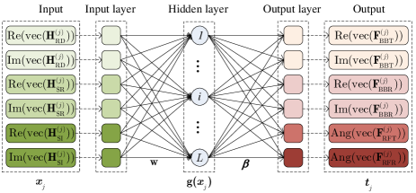
Figure 2: ELM network for HBF design at relay.

where $\bm{w}_{i}=[w_{i,1},\ldots,w_{i,N_{\text{I}}}]^{T}$ is the weight vector connecting the $i$-th hidden node and the input nodes, $\bm{\beta}=\left[\beta_{1},\ldots,\beta_{L}\right]^{T}\in\mathbb{R}^{L\times N_{\text{o}}}$, and $\beta_{i}=[\beta_{i,1},\ldots,\beta_{i,N_{\text{o}}}]^{T}$ is the weight vector connecting the $i$-th hidden node and the output nodes, and $b_{i}$ is the bias of the $i$-th hidden node. Considering all the samples in $\mathcal{D}$, we stack (31) to obtain the hidden-layer output as

$${\bf G}=\left[\begin{matrix}{\bf g}(\bm{x}_{1})\\ \vdots\\ {\bf g}(\bm{x}_{N})\end{matrix}\right]=\left[\begin{matrix}g_{1}(\bm{x}_{1})&\cdots&g_{L}(\bm{x}_{1})\\ \vdots&\cdots&\vdots\\ g_{1}(\bm{x}_{N})&\cdots&g_{L}(\bm{x}_{N})\end{matrix}\right]_{L\times N}.$$ (32)

Actually, we can regard ${\bf G}$ as the feature mapping from the training data, which maps the data from the $N_{\text{I}}$-dimensional space into the $L$-dimensional hidden-layer feature space.

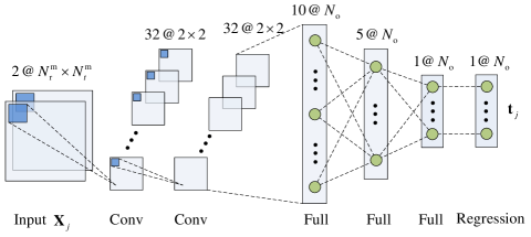
Figure 3: CNN network for HBF design at relay.

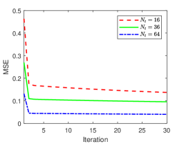
(a)

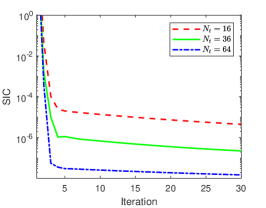
(b)

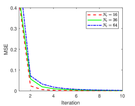
(c)

Figure 4: MSE and SIC performance for the proposed beamforming algorithms vs the number of iterations and different numbers of antennas, $N_{t}=N_{r}$, $N_{s}=2$ and $N_{\text{RFR}}=N_{\text{RFT}}=4$: (a) MSE for ADMM-based algorithms; (b) SIC performance for ADMM-based algorithms; (c) MSE for MM-based algorithms.

Since there is only one hidden layer in ELM, with randomized weights $\{\bm{w}_{i}\}$ and biases $\{b_{i}\}$, the goal is to tune the output weight $\bm{\beta}$ with training data $\mathcal{D}$ through minimizing the ridge regression problem

$$(\text{P}7):~{}\bm{\beta}^{*}=\arg\min_{\bm{\beta}}~{}\frac{\lambda}{2}\left\|{\bf G}\bm{\beta}-{\bf T}\right\|^{2}+\frac{1}{2}\left\|\bm{\beta}\right\|^{2},$$ (33)

where ${\bf T}=\left[\bm{t}_{1},\ldots,\bm{t}_{N}\right]^{T}_{N\times N_{\text{o}}}$ is the concatenated target, $\lambda$ is the trade-off parameter between the training error and the regularization. According to [37], the closed-form solution for (P7) is

$$\bm{\beta}^{*}={\bf G}^{T}\left(\frac{\bf{I}}{\lambda}+{\bf G}{\bf G}^{T}\right)^{-1}{\bf T},~{}~{}N\leq L,$$ (34)

or

$$\bm{\beta}^{*}=\left(\frac{\bf{I}}{\lambda}+{\bf G}^{T}{\bf G}\right)^{-1}{\bf G}^{T}{\bf T},~{}~{}N>L,$$ (35)

where $\bm{\beta}^{*}$ in (34) is derived for the case where the number of training samples is small, while $\bm{\beta}^{*}$ in (35) is derived for the case where the number of training samples is huge. From above, we can see that ELM is with very low complexity since there is only one layer’s parameters to be trained and the weight of output layer (i.e., $\bm{\beta}$ ) is given in closed-form.

IV-B FD mmwave beamforming design with CNN

Due to the advantages of data compression, CNN is another promising learning network to solve communication problems at the physical layer. Some latest CNN based HBF designs are presented in [17, 20], but these works are only for single-hop wireless communications. Based on the CNN-based hybrid beamforming model in [17, 20], we extend it to FD mmWave systems. The CNN-based architecture is shown in Fig. 3, which has a total eleven layers, including an input layer, two convolution layers, three fully connected layers, a regression output layer and four activation layers after each convolutional layer and fully connected layer. Detailed parameters in each layer are shown in Fig. 3. Different from ELM, the $j$-th input data ${\bf{X}}_{j}$ of CNN is a three-dimensional (3D) real matrix with size $N_{\text{r}}^{\text{m}}\times N_{\text{t}}^{\text{m}}\times 2$ where $N_{\text{t}}^{\text{m}}=\max(N_{t},n_{t})$ and $N_{\text{r}}^{\text{m}}=\max(N_{r},n_{r})$. We define the first channel of the input as the element-wise real value of the input channel matrix given by $[{\bf{X}}_{j}]_{:,:,1}=[\text{Re}(\overline{\bf{H}}^{(j)}_{\text{SR}}),\text{Re}(\overline{\bf{H}}^{(j)}_{\text{RD}}),\text{Re}(\overline{\bf{H}}^{(j)}_{\text{SI}})]$, and the second channel of the input as the element-wise imaginary value of the input channel matrix given by $[{\bf{X}}_{j}]_{:,:,2}=[\text{Im}(\overline{\bf{H}}^{(j)}_{\text{SR}}),\text{Im}(\overline{\bf{H}}^{(j)}_{\text{RD}}),\text{Im}(\overline{\bf{H}}^{(j)}_{\text{SI}})]$. The output of the CNN is the same as that of ELM, which can be obtained from Algorithm 2. More details of CNN can be found in [17].

V Numerical simulations

In this section, we will numerically evaluate the performance of the proposed MO and ADMM based HBF algorithm (MM-ADMM-HBF), ELM-based HBF method (ELM-HBF) and CNN-based HBF method (CNN-HBF). We compared our results with four benchmark algorithms: SI-free fully digital beamforming (Full-D), fully digital beamforming with SI (Full-D with SI), HD fully digital beamforming (HD Full-D) and OMP-based HBF method (OMP-HBF) [2]. The channel parameters are set to $N_{\text{c}}=5$, $N_{\text{p}}=10$, $d=\frac{\lambda}{2}$ and $\alpha_{k,l}\sim\mathcal{CN}(0,1)$[2]. The bandwidth of this system is $2$ GHz with central carrier frequency $f_{c}=28$ GHz. According to [2], the pathloss is $P_{\text{loss}}=61.5+20\log(r)+\varepsilon$ (dB) where $\varepsilon\sim N(0,5.8)$ and $r$ denotes the distance between transmitter and receiver. We assume that the distance between source and relay, and the distance between relay and destination are $r_{\text{sr}}=100$ m and $r_{\text{rd}}=100$ m, respectively. We assume that all nodes in FD mmWave systems have the same hardware constraints, and $N_{\text{t}}=n_{\text{t}}$, $N_{\text{r}}=n_{\text{r}}$, $N_{\text{RFR}}=N_{\text{RFD}}$, $N_{\text{s}}=n_{\text{s}}$ and $N_{\text{RFT}}=N_{\text{RFS}}$. In both training and testing stages, each channel realization is added by AWGN with different powers of $\text{SNR}_{\text{Train}}=\text{SNR}_{\text{Test}}\in\{15,20,25\}$ dB.

V-A Performance of ADMM and MM based beamforming

Fig. 4 summarizes the performance of proposed beamforming algorithms versus the number of iterations and different numbers of antennas. Fig. LABEL:sub@fig:4a shows the MSE performance (i.e., $\left\|{\bf F}_{\text{opt}}-{\bf F}_{\text{T}}{\bf F}_{\text{R}}^{H}\right\|_{\text{F}}^{2}$) of the ADMM based beamforming algorithm (Algorithm 1). We can observe a fast convergence of the proposed algorithm and the convergence rate decreases as the number of antennas increases. Results also show that the MSE of Algorithm 1 at convergence decreases as the number of antennas increases. Fig. LABEL:sub@fig:4b shows the SIC performance (i.e., ${\|{\bf F}_{\rm R}^{H}{\bf H}_{\rm SI}{\bf F}_{\rm T}\|}_{\rm{F}}^{2}$) of Algorithm 1. It is shown that the power of the SI decreases with increasing numbers of algorithmic iteration. We can also see that using a large number of antennas can eliminate SI faster. Fig. LABEL:sub@fig:4c shows the MSE performance (i.e., $\left\|\hat{\bf F}_{\text{opt}}-{\bf F}_{\text{RFT}}{\bf F}_{\text{BBT}}{\bf F}_{\text{BBR}}^{H}{\bf F}_{\text{RFR}}^{H}\right\|_{\text{F}}^{2}$) of the MM-based HBF algorithm (Algorithm 2). It is shown that a very fast convergence rate of Algorithm 2, even for the case with a large number of antennas (e.g., $N_{t}=64$).

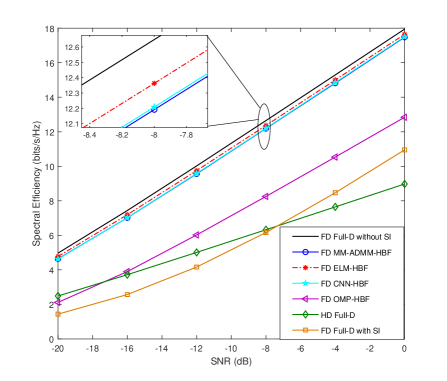
Figure 5: Spectral efficiency of various HBF algorithms vs SNR with $N_{t}=N_{r}=36$, $N_{\text{RFR}}=6$, $N_{\text{RFT}}=8$ and $N_{\text{s}}=2$.

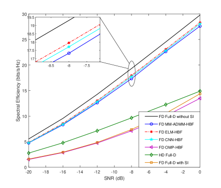
Figure 6: Spectral efficiency of various HBF algorithms vs SNR with $N_{t}=N_{r}=36$, $N_{\text{RFR}}=6$, $N_{\text{RFT}}=8$ and $N_{\text{s}}=4$.

V-B Hybrid beamforming performance

Fig. 5 and Fig. 6 show the spectral efficiency of the proposed HBF methods and existing methods versus SNR and different numbers of transmitting streams. From Fig. 5, we can see that the proposed MM-ADMM based HBF algorithm can approximately achieve the performance of fully digital beamforming without SI, which means that the proposed algorithm can achieve near-optimal HBF and guarantee efficient SIC. We can also see that the proposed algorithm significantly outperforms OMP based algorithm. The reason is that the OMP-based algorithm in [2] eliminates SI by adjusting the derived optimal beamformers, which will significantly degrade the spectral efficiency. Furthermore, the proposed CNN-based and ELM-based HBF methods outperform other methods. The performance of learning based methods is attributed to extracting the features of noisy input data (i.e., imperfect channels for different links) and be robust to the imperfect channels. We can see that all proposed methods can approximately achieve twice the spectral efficiency to the HD system. Fig. 6 shows that our proposed methods can also achieve high spectral efficiency with increasing number of transmitting streams. However, the spectral efficiency of OMP-based algorithm becomes even lower than the FD fully-digital beamforming with SI. The reason is that OMP-based algorithm can eliminate SI only when $N_{\text{RFT}}\geq N_{\text{RFR}}+N_{\text{s}}$. Comparing the result in Fig. 5 to that in Fig. 6, we can find that the spectral efficiency is significantly increased as the number of transmitting streams increases.

Fig. 7 shows two groups of spectral efficiency with different numbers of antennas. In each group, simulation results of three proposed methods together with OMP-HBF and Full-D beamforming methods are presented. It is shown that the spectral efficiency increases as the number of antennas increases, and the gap of the results within a group decreases simultaneously. Moreover, the proposed methods can achieve higher spectral efficiency than the OMP-HBF method. We can also see that the proposed methods can approximately achieve the performance of Full-D beamforming without SI when $N_{\textbf{t}}=N_{\textbf{r}}=64$. Finally, the proposed learning based HBF methods (i.e., ELM-HBF and CNN-HBF) outperform the optimization-based HBF methods (i.e., OMP-HBF and MM-ADMM-HBF).

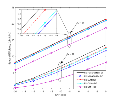
Figure 7: Spectral efficiency of various HBF algorithms vs SNR and different numbers of antennas with $N_{t}=N_{r}$, $N_{\text{RFR}}=4$, $N_{\text{RFT}}=6$.

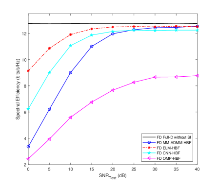
Figure 8: Spectral efficiency of various HBF algorithms vs $\text{SNR}_{\text{Test}}$ with $N_{t}=N_{r}=36$, $N_{\text{RFR}}=4$, $N_{\text{RFT}}=6$ and $\text{SNR}=-8$ dB.

TABLE I: Spectral Efficiency (bits/s/Hz), Training and Prediction Time Comparison

Nt	MM-ADMM		OMP		CNN			ELM
								Sigmoid Node			Multiquadrics RBF Node			PReLU Node
	Prediction Time (s)	SE	Prediction Time (s)	SE	Prediction Time (s)	Training Time (s)	SE	Prediction Time (s)	Training Time (s)	SE	Prediction Time (s)	Training Time (s)	SE	Prediction Time (s)	Training Time (s)	SE
16	0.1920	6.6393	0.0291	4.1733	0.0063	315.51	6.8146	0.0626	66.98	7.1410	0.0249	59.59	7.1491	0.0056	1.5791	7.1291
36	0.6112	11.8715	0.3103	8.1470	0.0134	963.58	11.8818	0.1859	275.23	12.2395	0.1338	213.99	12.3890	0.0126	2.9624	12.3569
64	1.7422	15.5430	1.2210	11.5962	0.0349	3714.3	15.7585	0.6681	1225.6	15.8468	0.5830	1146.1	15.9355	0.0530	6.1633	15.8555

In order to evaluate the performance of algorithms on the robustness, we present the spectral efficiency of various HBF algorithms versus different noise levels (i.e., $\text{SNR}_{\text{Test}}$) in Fig. 8. Note that SI-free fully digital beamforming (Full-D) is fed with perfect CSI which can achieve the best performance. From Fig. 8, we can see that the performance of all methods increase with increasing $\text{SNR}_{\text{Test}}$. We can also see that both ELM-HBF and CNN-HBF are more robust against the corruption in the channel data compared to other methods. The reason is that proposed learning based methods estimate the beamformers by extracting the features of noisy input data, while MM-ADMM and OMP methods require optimal digital beamformers which are derived from noisy channels. Furthermore, it is shown that ELM-HBF outperforms CNN-HBF. The reason is that the optimal weight matrix of ELM network can be derived in a close-form, while the multi-layer parameters of CNN are hard to be optimized. Finally, we can see that the ELM-HBF can approximately achieve optimal as $\text{SNR}_{\text{Test}}$ increases.

V-C Computational Complexity

In this part, we measure the computation time of our proposed HBF approaches and compared them with OMP-HBF. The computation time of a learning machine includes offline training time and online prediction time. Since the learning network performance and training time are relative to the activation function in the hidden node, we make a performance comparison among following three common activation functions for ELM:

(1) Sigmoid function

$$g(\bm{w},\bm{x},b)=\frac{1}{1+\exp(-\bm{w}^{T}\bm{x}-b)};$$ (36)

(2) Multi-quadratic radial basis function (RBF)

$$g(\bm{w},\bm{x},b)=\sqrt{\left\|\bm{x}-\bm{w}\right\|^{2}+b^{2}};$$ (37)

(3) Parametric rectified linear unit (PReLU) function

$$g(\bm{w},\bm{x},a)=\max(0,\bm{w}^{T}\bm{x})+a\min(0,\bm{w}^{T}\bm{x}).$$ (38)

For CNN, the multi-layer structure will lead to high computational complexity and a simple rectified linear unit (ReLU) activation function (i,e, $g(\bm{w},\bm{x})=\max(0,\bm{w}^{T}\bm{x})$) is commonly used to reduce the training complexity. Results in [20, 21, 17] show that CNN with ReLU can achieve good classification performance. Thus, we consider ReLU activation function for CNN. We select $N_{\text{s}}=2$, $N_{\text{RFR}}=4$, $N_{\text{RFT}}=6$ and $\text{SNR}=-8$ dB. $1000$ channel samples for $10$ channel realizations are fed into the learning machines, and $100$ channel samples are used for testing. For different approaches, we summarize the spectral efficiency (SE), training time and prediction time in Table I.

We can see that the proposed ELM-HBF and CNN-HBF methods can achieve higher spectral efficiency and less prediction time than the optimization-based methods (i.e., MM-ADMM and OMP). In addition, we can observe that the prediction time increases with the number of antennas. It is shown that CNN and ELM with PReLU can achieve very low prediction time (e.g., less than $0.06$ s for the case with $N_{\text{t}}=64$). Although ELM with multi-quadric RBF can achieve a slightly higher spectral efficiency than that with PReLU, it requires almost ten times the prediction time and a hundred times the training time compared to that with PReLU. For instance, the training time of multi-quadric RBF is about $1146.1$ s while it is about $6.1633$ s of PReLU for the case with $N_{\textbf{t}}=64$. Results show that CNN always spends longer training time and achieves lower spectral efficiency than ELM. For instance, CNN takes about 600 times the training time compared to ELM with PReLU for the case with $N_{\textbf{t}}=64$.

VI Conclusions

We proposed two learning schemes for HBF design of FD mmWave systems, i.e., ELM-HBF and CNN-HBF. The learning machines use noisy channels of different nodes as inputs and output the hybrid beamformers. To provide accurate labels of input channel data, we first proposed an ADMM based algorithm to achieve SIC beamforming, and then proposed an MM based algorithm for joint transmitting and receiving HBF optimization. The convergence and complexity for both algorithms were analyzed. The effectiveness of the proposed methods was evaluated through several experiments. Results illustrate that both ADMM and MM based algorithms can converge and the SI can be effectively suppressed. Results also show that both proposed ELM-HBF and CNN-HBF methods can achieve higher spectral efficiency and much lower prediction time than the convectional optimization-based methods. Furthermore, the proposed learning based methods can achieve more robust HBF performance than conventional methods. In addition, ELM-HBF with PReLU activation function can achieve much lower training time than that with Sigmoid or RBF activation function. Since ELM-HBF can achieve much lower computation time and more robust HBF performance than CNN-HBF, it might be more efficient to use ELM-HBF for practical implementation.

Appendix A Proof of Theorem 3

To prove the convergence of Algorithm 2, we first analyze the convergence of the MM algorithm when calculating ${\bf F}_{\text{RFT}}^{(k_{\text{o}}+1)}$ in step 6. According to the majorizer of $J({\bf F}_{\text{RFT}};{\bf Y}_{\text{T}})$ in (22), we have the following four properties,

$$J\left({\bf F}_{\text{RFT}}^{\left(k_{\text{i}}\right)};{\bf Y}_{\text{T}}^{(k_{\text{o}})}\right) =\bar{J}\left({\bf F}_{\text{RFT}}^{(k_{\text{i}})};{\bf Y}_{\text{T}}^{(k_{\text{o}})},{\bf F}_{\text{RFT}}^{(k_{\text{i}})}\right),$$ (39a)

$$\nabla_{{\bf F}_{\text{RFT}}}J\left({\bf F}_{\text{RFT}};{\bf Y}_{\text{T}}^{(k_{\text{o}})}\right) =\nabla_{{\bf F}_{\text{RFT}}}\bar{J}\left({\bf F}_{\text{RFT}};{\bf Y}_{\text{T}}^{(k_{\text{o}})},{\bf F}_{\text{RFT}}^{(k_{\text{i}})}\right),$$ (39b)

$$J\left({\bf F}_{\text{RFT}}^{(k_{\text{i}}+1)};{\bf Y}_{\text{T}}^{(k_{\text{o}})}\right) \mathop{\leq}\limits^{(a)}\bar{J}\left({\bf F}_{\text{RFT}}^{(k_{\text{i}}+1)};{\bf Y}_{\text{T}}^{(k_{\text{o}})},{\bf F}_{\text{RFT}}^{(k_{\text{i}})}\right),$$ (39c)

$$\bar{J}\left({\bf F}_{\text{RFT}}^{(k_{\text{i}}+1)};{\bf Y}_{\text{T}}^{(k_{\text{o}})},{\bf F}_{\text{RFT}}^{(k_{\text{i}})}\right) \mathop{\leq}\limits^{(b)}\bar{J}\left({\bf F}_{\text{RFT}}^{(k_{\text{i}})};{\bf Y}_{\text{T}}^{(k_{\text{o}})},{\bf F}_{\text{RFT}}^{(k_{\text{i}})}\right),$$ (39d)

where (a) follows from $\lambda_{\text{T}}{\bf I}\geq{\bf Q}_{\text{T}}$, (b) follows from $\bar{J}({\bf F}_{\text{RFT}}^{(k_{\text{i}}+1)};{\bf Y}_{\text{T}}^{(k_{\text{o}})},{\bf F}_{\text{RFT}}^{(k_{\text{i}})})=\mathop{\min}\limits_{{\bf F}_{\text{RFT}}}\bar{J}({\bf F}_{\text{RFT}};{\bf Y}_{\text{T}}^{(k_{\text{o}})},{\bf F}_{\text{RFT}}^{(k_{\text{i}})})$, and ${\bf Y}_{\text{T}}^{(k_{\text{o}})}={\bf F}_{\text{BBT}}^{(k_{\text{o}}+1)}{\bf F}_{\text{BBR}}^{H(k_{\text{o}})}{\bf F}_{\text{RFR}}^{H(k_{\text{o}})}$. Based on properties (39a), (39c) and (39d), we obtain

$$\begin{split}J\left({\bf F}_{\text{RFT}}^{(k_{\text{i}}+1)};{\bf Y}_{\text{T}}^{(k_{\text{o}})}\right)&\leq\bar{J}\left({\bf F}_{\text{RFT}}^{(k_{\text{i}}+1)};{\bf Y}_{\text{T}}^{(k_{\text{o}})},{\bf F}_{\text{RFT}}^{(k_{\text{i}})}\right)\\ &\leq\bar{J}\left({\bf F}_{\text{RFT}}^{(k_{\text{i}})};{\bf Y}_{\text{T}}^{(k_{\text{o}})},{\bf F}_{\text{RFT}}^{(k_{\text{i}})}\right)\\ &=J\left({\bf F}_{\text{RFT}}^{(k_{\text{i}})};{\bf Y}_{\text{T}}^{(k_{\text{o}})}\right).\end{split}$$ (40)

Thus, $\{J({\bf F}_{\text{RFT}}^{(k_{\text{i}})};{\bf Y}_{\text{T}}^{(k_{\text{o}})})\}$ is a non-increasing sequence and thus it converges since $J({\bf F}_{\text{RFT}};{\bf Y}_{\text{T}})$ is lower bounded. Further, since $J({\bf F}_{\text{RFT}};{\bf Y}_{\text{T}}^{(k_{\text{o}})})$ and $\bar{J}({\bf F}_{\text{RFT}};{\bf Y}_{\text{T}}^{(k_{\text{o}})},{\bf F}_{\text{RFT}}^{(k_{\text{i}})})$ have the same gradient at point ${\bf F}_{\text{RFT}}^{(k_{\text{i}})}\in\mathcal{F}_{\text{RFT}}$ according to (39b), ${\bf F}_{\text{RFT}}^{(k_{\text{i}})}$ can converge to a stationary point solution of original problem (P4). After the converge of step 6, we have $J({\bf F}_{\text{RFT}}^{(k_{\text{o}}+1)};{\bf Y}_{\text{T}}^{(k_{\text{o}})})\leq J({\bf F}_{\text{RFT}}^{(k_{\text{o}})};{\bf Y}_{\text{T}}^{(k_{\text{o}})})$. Similarly, the convergence of the MM algorithm when calculating ${\bf F}_{\text{RFR}}^{(k_{\text{o}})}$ in step 14 can be proved with the following inequalities

$$\begin{split}J\left({\bf F}_{\text{RFR}}^{(k_{\text{i}}+1)};{\bf Y}_{\text{R}}^{(k_{\text{o}}+1)}\right)&\leq\tilde{J}\left({\bf F}_{\text{RFR}}^{(k_{\text{i}}+1)};{\bf Y}_{\text{R}}^{(k_{\text{o}}+1)},{\bf F}_{\text{RFR}}^{(k_{\text{i}})}\right)\\ &\leq\tilde{J}\left({\bf F}_{\text{RFR}}^{(k_{\text{i}})};{\bf Y}_{\text{R}}^{(k_{\text{o}}+1)},{\bf F}_{\text{RFR}}^{(k_{\text{i}})}\right)\\ &=J\left({\bf F}_{\text{RFR}}^{(k_{\text{i}})};{\bf Y}_{\text{T}}^{(k_{\text{o}}+1)}\right),\end{split}$$ (41)

where ${\bf Y}_{\text{R}}^{(k_{\text{o}}+1)}={\bf F}_{\text{RFT}}^{(k_{\text{o}}+1)}{\bf F}_{\text{BBT}}^{H(k_{\text{o}}+1)}{\bf F}_{\text{BBR}}^{H(k_{\text{o}}+1)}$. After the converge of step 14, we obtain $J({\bf F}_{\text{RFR}}^{(k_{\text{o}}+1)};{\bf Y}_{\text{R}}^{(k_{\text{o}}+1)})\leq J({\bf F}_{\text{RFR}}^{(k_{\text{o}})};{\bf Y}_{\text{R}}^{(k_{\text{o}}+1)})$. Then, based on above observations, we have

$$\begin{split}&J\left({\bf F}_{\text{RFT}}^{(k_{\text{o}})},{\bf F}_{\text{BBT}}^{(k_{\text{o}})},{\bf F}_{\text{BBR}}^{(k_{\text{o}})},{\bf F}_{\text{RFR}}^{(k_{\text{o}})}\right)=J\left({\bf F}_{\text{RFR}}^{(k_{\text{o}})};{\bf F}_{\text{BBT}}^{(k_{\text{o}})}{\bf F}_{\text{BBR}}^{H(k_{\text{o}})}{\bf F}_{\text{RFR}}^{H(k_{\text{o}})}\right)\\ &\qquad\qquad\qquad\qquad\quad\mathop{\geq}\limits^{(a)}J\left({\bf F}_{\text{RFT}}^{(k_{\text{o}})};{\bf F}_{\text{BBT}}^{(k_{\text{o}}+1)}{\bf F}_{\text{BBR}}^{H(k_{\text{o}})}{\bf F}_{\text{RFR}}^{H(k_{\text{o}})}\right)\\ &\qquad\qquad\qquad\quad\qquad\mathop{\geq}\limits^{(b)}J\left({\bf F}_{\text{RFT}}^{(k_{\text{o}}+1)};{\bf F}_{\text{BBT}}^{(k_{\text{o}}+1)}{\bf F}_{\text{BBR}}^{H(k_{\text{o}})}{\bf F}_{\text{RFR}}^{H(k_{\text{o}})}\right)\\ &\qquad\qquad\qquad\quad\qquad=J\left({\bf F}_{\text{RFR}}^{(k_{\text{o}})};{\bf F}_{\text{RFT}}^{(k_{\text{o}}+1)}{\bf F}_{\text{BBT}}^{H(k_{\text{o}}+1)}{\bf F}_{\text{BBR}}^{H(k_{\text{o}})}\right)\\ &\qquad\qquad\qquad\quad\qquad\mathop{\geq}\limits^{(c)}J\left({\bf F}_{\text{RFR}}^{(k_{\text{o}})};{\bf F}_{\text{RFT}}^{(k_{\text{o}}+1)}{\bf F}_{\text{BBT}}^{H(k_{\text{o}}+1)}{\bf F}_{\text{BBR}}^{H(k_{\text{o}}+1)}\right)\\ &\qquad\qquad\qquad\quad\qquad\mathop{\geq}\limits^{(d)}J\left({\bf F}_{\text{RFR}}^{(k_{\text{o}}+1)};{\bf F}_{\text{RFT}}^{(k_{\text{o}}+1)}{\bf F}_{\text{BBT}}^{H(k_{\text{o}}+1)}{\bf F}_{\text{BBR}}^{H(k_{\text{o}}+1)}\right)\\ &\qquad\qquad\qquad\quad\qquad=J\left({\bf F}_{\text{RFT}}^{(k_{\text{o}}+1)},{\bf F}_{\text{BBT}}^{(k_{\text{o}}+1)},{\bf F}_{\text{BBR}}^{(k_{\text{o}}+1)},{\bf F}_{\text{RFR}}^{(k_{\text{o}}+1)}\right),\\ \end{split}$$ (42)

where (a) and (c) respectively follow from

$$\begin{split}J\left({\bf F}_{\text{RFT}}^{(k_{\text{o}})};{\bf F}_{\text{BBT}}^{(k_{\text{o}}+1)}\right.&\left.{\bf F}_{\text{BBR}}^{H(k_{\text{o}})}{\bf F}_{\text{RFR}}^{H(k_{\text{o}})}\right)\\ &=\mathop{\min}\limits_{{\bf F}_{\text{BBT}}}J\left({\bf F}_{\text{RFT}}^{(k_{\text{o}})};{\bf F}_{\text{BBT}}{\bf F}_{\text{BBR}}^{H(k_{\text{o}})}{\bf F}_{\text{RFR}}^{H(k_{\text{o}})}\right),\end{split}$$ (43)

and

$$\begin{split}J\left({\bf F}_{\text{RFR}}^{(k_{\text{o}})};{\bf F}_{\text{RFT}}^{(k_{\text{o}}+1)}\right.&\left.{\bf F}_{\text{BBT}}^{H(k_{\text{o}}+1)}{\bf F}_{\text{BBR}}^{H(k_{\text{o}}+1)}\right)\\ &=\mathop{\min}\limits_{{\bf F}_{\text{BBR}}}J\left({\bf F}_{\text{RFR}}^{(k_{\text{o}})};{\bf F}_{\text{RFT}}^{(k_{\text{o}}+1)}{\bf F}_{\text{BBT}}^{H(k_{\text{o}}+1)}{\bf F}_{\text{BBR}}^{H}\right),\end{split}$$ (44)

(b) and (d) follow from (40) and (41), respectively.

Thus, $\{J({\bf F}_{\text{RFT}}^{(k_{\text{o}})},{\bf F}_{\text{BBT}}^{(k_{\text{o}})},{\bf F}_{\text{BBR}}^{(k_{\text{o}})},{\bf F}_{\text{RFR}}^{(k_{\text{o}})})\}$ is a non-increasing sequence and thus it converges since $J({\bf F}_{\text{RFT}},{\bf F}_{\text{BBT}},{\bf F}_{\text{BBR}},{\bf F}_{\text{RFR}})$ is lower bounded. The proof of convergence of Algorithm 2 is completed.

For Algorithm 2, the main complexity in each iteration includes the following three parts:

1) Compute ${\bf F}_{\text{BBT}}$ and ${\bf F}_{\text{BBR}}$. The complexity of pseudo inversion can be measured by the complexity of singular value decomposition. Thus, the main complexity for this part is $\mathcal{O}(n_{\text{t}}N_{\text{RFT}}^{2}+n_{\text{r}}N_{\text{RFR}}^{2}+n_{\text{s}}^{2}(n_{\text{r}}+n_{\text{t}}))$.

2) Compute ${\bf F}_{\text{RFT}}$ and ${\bf F}_{\text{RFR}}$ with MM methods. The main complexity comes from finding the maximum eigenvalue of ${\bf Q}_{\text{T}}$ and the maximum eigenvalue of ${\bf Q}_{\text{R}}$. The main complexity of this part is $\mathcal{O}((n_{\text{r}}N_{\text{RFR}})^{3}+(n_{\text{t}}N_{\text{RFT}})^{3})$.

Thus, the main complexity for Algorithm 2 is given by $\mathcal{O}(K_{\text{out}}(K_{\text{in}}((n_{\text{r}}N_{\text{RFR}})^{3}+(n_{\text{t}}N_{\text{RFT}})^{3})+n_{\text{t}}N_{\text{RFT}}^{2}+n_{\text{r}}N_{\text{RFR}}^{2}+n_{\text{s}}^{2}(n_{\text{r}}+n_{\text{t}})))$.

References

- [1] M. Xiao, S. Mumtaz, Y. Huang, L. Dai, Y. Li, M. Matthaiou, G. K. Karagiannidis, E. Björnson, K. Yang, C. I, and A. Ghosh, “Millimeter wave communications for future mobile networks,” IEEE Journal on Selected Areas in Communications, vol. 35, pp. 1909–1935, Sep. 2017.
- [2] Y. Zhang, M. Xiao, S. Han, M. Skoglund, and W. Meng, “On precoding and energy efficiency of full-duplex millimeter-wave relays,” IEEE Transactions on Wireless Communications, vol. 18, no. 3, pp. 1943–1956, 2019.
- [3] X. Wang, L. Kong, F. Kong, F. Qiu, M. Xia, S. Arnon, and G. Chen, “Millimeter wave communication: A comprehensive survey,” IEEE Communications Surveys Tutorials, vol. 20, pp. 1616–1653, thirdquarter 2018.
- [4] O. El Ayach, S. Rajagopal, S. Abu-Surra, Z. Pi, and R. W. Heath, “Spatially sparse precoding in millimeter wave MIMO systems,” IEEE transactions on wireless communications, vol. 13, no. 3, pp. 1499–1513, 2014.
- [5] T. S. Rappaport, Y. Xing, G. R. MacCartney, A. F. Molisch, E. Mellios, and J. Zhang, “Overview of millimeter wave communications for fifth-generation (5G) wireless networks—With a focus on propagation models,” IEEE Transactions on Antennas and Propagation, vol. 65, no. 12, pp. 6213–6230, 2017.
- [6] I. Atzeni and M. Kountouris, “Full-duplex MIMO small-cell networks with interference cancellation,” IEEE Transactions on Wireless Communications, vol. 16, no. 12, pp. 8362–8376, 2017.
- [7] S. Han, Y. Zhang, W. Meng, and Z. Zhang, “Precoding design for full-duplex transmission in millimeter wave relay backhaul,” Mobile Networks and Applications, vol. 23, no. 5, pp. 1416–1426, 2018.
- [8] S. K. Sharma, T. E. Bogale, L. B. Le, S. Chatzinotas, X. Wang, and B. Ottersten, “Dynamic spectrum sharing in 5G wireless networks with full-duplex technology: Recent advances and research challenges,” IEEE Communications Surveys & Tutorials, vol. 20, no. 1, pp. 674–707, 2017.
- [9] T. Dinc and H. Krishnaswamy, “Millimeter-wave full-duplex wireless: Applications, antenna interfaces and systems,” in 2017 IEEE Custom Integrated Circuits Conference (CICC), pp. 1–8, IEEE, 2017.
- [10] K. Satyanarayana, M. El-Hajjar, P.-H. Kuo, A. Mourad, and L. Hanzo, “Hybrid beamforming design for full-duplex millimeter wave communication,” IEEE Transactions on Vehicular Technology, vol. 68, no. 2, pp. 1394–1404, 2018.
- [11] Y. He, X. Yin, and H. Chen, “Spatiotemporal characterization of self-interference channels for 60-GHz full-duplex communication,” IEEE Antennas and Wireless Propagation Letters, vol. 16, pp. 2220–2223, 2017.
- [12] H. Abbas and K. Hamdi, “Full duplex relay in millimeter wave backhaul links,” in 2016 IEEE Wireless Communications and Networking Conference, pp. 1–6, IEEE, 2016.
- [13] Z. Xiao, P. Xia, and X.-G. Xia, “Full-duplex millimeter-wave communication,” IEEE Wireless Communications, vol. 24, no. 6, pp. 136–143, 2017.
- [14] H. Huang, J. Yang, H. Huang, Y. Song, and G. Gui, “Deep learning for super-resolution channel estimation and DOA estimation based massive MIMO system,” IEEE Transactions on Vehicular Technology, vol. 67, no. 9, pp. 8549–8560, 2018.
- [15] Y. Long, Z. Chen, J. Fang, and C. Tellambura, “Data-driven-based analog beam selection for hybrid beamforming under mm-wave channels,” IEEE Journal of Selected Topics in Signal Processing, vol. 12, no. 2, pp. 340–352, 2018.
- [16] N. Samuel, T. Diskin, and A. Wiesel, “Deep MIMO detection,” in 2017 IEEE 18th International Workshop on Signal Processing Advances in Wireless Communications (SPAWC), pp. 1–5, IEEE, 2017.
- [17] A. M. Elbir, “CNN-based precoder and combiner design in mmWave MIMO systems,” IEEE Communications Letters, vol. 23, no. 7, pp. 1240–1243, 2019.
- [18] H. Huang, Y. Song, J. Yang, G. Gui, and F. Adachi, “Deep-learning-based millimeter-wave massive MIMO for hybrid precoding,” IEEE Transactions on Vehicular Technology, vol. 68, no. 3, pp. 3027–3032, 2019.
- [19] T. Lin and Y. Zhu, “Beamforming design for large-scale antenna arrays using deep learning,” IEEE Wireless Communications Letters, 2019.
- [20] X. Bao, W. Feng, J. Zheng, and J. Li, “Deep CNN and Equivalent Channel Based Hybrid Precoding for mmWave Massive MIMO Systems,” IEEE Access, vol. 8, pp. 19327–19335, 2020.
- [21] A. M. Elbir and K. V. Mishra, “Joint Antenna Selection and Hybrid Beamformer Design using Unquantized and Quantized Deep Learning Networks,” IEEE Transactions on Wireless Communications, 2019.
- [22] X. Yu, J.-C. Shen, J. Zhang, and K. B. Letaief, “Alternating minimization algorithms for hybrid precoding in millimeter wave MIMO systems,” IEEE Journal of Selected Topics in Signal Processing, vol. 10, no. 3, pp. 485–500, 2016.
- [23] T. Lin, J. Cong, Y. Zhu, J. Zhang, and K. B. Letaief, “Hybrid beamforming for millimeter wave systems using the MMSE criterion,” IEEE Transactions on Communications, vol. 67, no. 5, pp. 3693–3708, 2019.
- [24] F. Sohrabi and W. Yu, “Hybrid digital and analog beamforming design for large-scale antenna arrays,” IEEE Journal of Selected Topics in Signal Processing, vol. 10, no. 3, pp. 501–513, 2016.
- [25] J. Lee and Y. H. Lee, “AF relaying for millimeter wave communication systems with hybrid RF/baseband MIMO processing,” in 2014 IEEE International Conference on Communications (ICC), pp. 5838–5842, IEEE, 2014.
- [26] C. G. Tsinos, S. Chatzinotas, and B. Ottersten, “Hybrid analog-digital transceiver designs for mmwave amplify-and-forward relaying systems,” in 2018 41st International Conference on Telecommunications and Signal Processing (TSP), pp. 1–6, IEEE, 2018.
- [27] S. Boyd, N. Parikh, E. Chu, B. Peleato, J. Eckstein, et al., “Distributed optimization and statistical learning via the alternating direction method of multipliers,” Foundations and Trends in Machine learning, vol. 3, no. 1, pp. 1–122, 2011.
- [28] Y. Sun, P. Babu, and D. P. Palomar, “Majorization-minimization algorithms in signal processing, communications, and machine learning,” IEEE Transactions on Signal Processing, vol. 65, no. 3, pp. 794–816, 2016.
- [29] L. Wu, P. Babu, and D. P. Palomar, “Transmit waveform/receive filter design for MIMO radar with multiple waveform constraints,” IEEE Transactions on Signal Processing, vol. 66, no. 6, pp. 1526–1540, 2017.
- [30] A. Arora, C. G. Tsinos, S. Chatzinotas, B. Ottersten, et al., “Hybrid Transceivers Design for Large-Scale Antenna Arrays Using Majorization-Minimization Algorithms,” IEEE Transactions on Signal Processing, 2019.
- [31] P. Comon and G. H. Golub, “Tracking a few extreme singular values and vectors in signal processing,” Proceedings of the IEEE, vol. 78, no. 8, pp. 1327–1343, 1990.
- [32] P. L. Bartlett, “The sample complexity of pattern classification with neural networks: the size of the weights is more important than the size of the network,” IEEE Transactions on Information Theory, vol. 44, pp. 525–536, March 1998.
- [33] K. Hornik, M. Stinchcombe, H. White, et al., “Multilayer feedforward networks are universal approximators.,” Neural networks, vol. 2, no. 5, pp. 359–366, 1989.
- [34] Y. Ye, M. Xiao, and M. Skoglund, “Decentralized multi-task learning based on extreme learning machines,” arXiv preprint arXiv:1904.11366, 2019.
- [35] T. D. Sanger, “Optimal unsupervised learning in a single-layer linear feedforward neural network,” Neural networks, vol. 2, no. 6, pp. 459–473, 1989.
- [36] G.-B. Huang, Q.-Y. Zhu, and C.-K. Siew, “Extreme learning machine: theory and applications,” Neurocomputing, vol. 70, no. 1-3, pp. 489–501, 2006.
- [37] G.-B. Huang, H. Zhou, X. Ding, and R. Zhang, “Extreme learning machine for regression and multiclass classification,” IEEE Transactions on Systems, Man, and Cybernetics, Part B (Cybernetics), vol. 42, no. 2, pp. 513–529, 2011.
- [38] G.-B. Huang, D. H. Wang, and Y. Lan, “Extreme learning machines: a survey,” International journal of machine learning and cybernetics, vol. 2, no. 2, pp. 107–122, 2011.