Beat Detection and Automatic Annotation of the Music of Bharatanatyam Dance using Speech Recognition Techniques

Abstract

Bharatanatyam, an Indian Classical Dance form, represents the rich cultural heritage of India. Analysis and recognition of such dance forms are critical for preservation of cultural heritage. Like in most dance forms, a Bharatanatyam dancer performs in synchronization with structured rhythmic music, called Sollukattu, that comprises instrumental beats and vocalized utterances (bols) to create a rhythmic music structure. Computer analysis of Bharatanatyam, therefore, requires structural analysis of Sollukattus. In this paper, we use speech processing techniques to recognize bols. Exploiting the predefined structures of Sollukattus and the detected bols, we recognize the Sollukattu. We estimate the tempo period by two methods. Finally we generate a complete annotation of the audio signal by beat marking. For this we also use information of beats detected from the onset envelope of a Sollukattu signal [13]. For training and test, we create a data set for Sollukattus and annotate them. We achieve 85% accuracy in bol recognition, 95% in Sollukattu recognition, 96% in tempo period estimation, and over 90% in beat marking. This is the maiden attempt to fully structurally analyze the music of an Indian Classical Dance form and the use of speech processing techniques for beat marking.

Keywords Bharatanatyam Dance, Ontological model, Heritage preservation, Indian Classical Dance, Beat Marking, Audio annotation, Gaussian Mixture Model, Tempo estimation, Comb filter, MFCC feature

1 Introduction

Bharatanatyam, an Indian Classical Dance (ICD) form, represents the rich cultural heritage of India. Modeling, analysis, recognition and interpretation of such dance forms are important to preserve intangible cultural heritage by dance transcription and automatic annotation of dance videos, to create dance tutoring systems, to create animation with avatars, and so on. Bharatanatyam has a complex language in which the dancers communicate to their audience by telling a story through craftily synchronized visual (postures, gestures, and movements), auditory (beats and bols or utterances), and textual (narration and lyrics) information.

Like in most dance forms, a Bharatanatyam dancer performs in sync with structured rhythmic music, called Sollukattu. Specific rhythms are created in a Sollukattu with instrumental beats using Tatta Kazhi, Mridangam etc. Monosyllabic vocal utterances, called bols, often accentuate the beats and serve as cues for actions of the dancer. Vocal music may also be used for embellishment. Analysis of a Bharatanatyam performance, therefore, is critically dependent on understanding the structures of Sollukattus.

In this paper, we attempt to automatically annotate the audio signal of a Sollukattu by detecting its beats, recognizing the accompanying bols, recognizing the Sollukattu, estimating its tempo period, and marking the time-stamps of the beats on the signal. The annotation may be used to denote interesting events like key postures and elemental motion elements, on the Bharatanatyam dance video and segmented for further visual analysis.

To keep the complexity of the problem manageable, we work only with Adavus of Bharatanatyam. An Adavu is a basic unit of Bharatanatyam performance comprising well-defined sets of postures, gestures, movements and their transitions, and is typically used to train the dancers. There are 58 Adavus commonly used in Bharatanatyam and each Adavu is synchronized with one of the 23 Sollukattus. Analysis of a Sollukattu is a challenging task because it may contain various sources of noise and there are several events (like full-beat, half-beat, and bol) in the signal to detect. The generation of the music itself may be imperfect due to the lack of skill of the beater or simple human error and fatigue. So we engage a combination of signal processing and speech recognition techniques for the tasks.

We start with a brief look into various approaches to similar problems in Sec. 2. We classify the events for a Sollukattu in Sec. 3 and present an ontological model. The problem is formally stated in Sec. 4 and the approach to solution is outlined. Sec. 5 presents the data set and annotation. A recognizer for bols is discussed in Sec. 6 along with the signature of audio signals. Sec. 7 introduces the signature of a Sollukattu and then presents a recognizer for Sollukattus. Tempo period is estimated in Sec. 8. Based on the analysis and outputs from the earlier sections, we present an algorithm to mark the beats (annotate) on a Sollukattu signal in Sec. 9. Finally, we conclude in Sec. 10.

2 Related Work & Approach of Analysis

Music is usually created by various instruments like idiophones (percussion instruments), membranophones (vibrating membranes), aerophones (wind instruments), or chordophones (stringed instruments). Often it is accompanied by human voice which may either function as an instrument, or render speech in melody and harmony to the underlying music, or both. Music usually has rhythm that defines its pattern in time and comprises pitch of high and low tones. Rhythm defines the way the musical sounds and silences are put together in a sequence and often has regular beats. When accompanied by speech-like vocal line (or song), music usually carries a lyrics composed of verses. While there exist several variations to these notions of music and multitude of more parameters (like dynamics, timbre) to define it; the above is a typical characterization of music used in research on acoustic musical signals. Consequently, research has been focused mainly in two areas: (1) Structural Analysis of Music (beat detection, tempo estimation, beat tracking etc.) and (2) Semantic Analysis of Lyrics (song retrieval, segmentation, labeling, and recognition, genre classification, transcription of lyrics, etc.). We take a brief look into these before putting our work into context.

For structural analysis of music, various algorithms for beat detection, tempo estimation, and beat tracking have been reported. Many of these, like [3], [5], and [6], work on a common framework where first the onset locations are extracted from a time-frequency or sub-band analysis of the signal by using a filter bank or Fast Fourier Transform (FFT), and then a periodicity estimation algorithm is employed to determine the rate at which these events occur. There are variants of this approach. For example, Peeters et al. [16] propose a probabilistic framework for estimation of beat and downbeat locations in an audio by considering the tempo period and meter as input. The variations notwithstanding, we observe that researchers mostly do not consider the vocal sound, if present in the music, for structural analysis.

Semantic analysis, on the other hand, is primarily undertaken for songs that may consist of musically relevant sounds by the human voice along with the instrumental sound. For example, Mesaros et al. [15] recognize phonemes and words in the audio to align textual lyrics and to retrieve songs, Cheng et al. [2] process lyrics for extracting semantically meaningful segments, Berenzweig et al. [1] locate singing voice segments in music using a speech recognition system, Goto et al. [8] design for speech completion and spotter interface in a background-music playback system, and Scheirer et al. [19] present large selection of signal-level features to discriminate regular speech from music. Most of these use different speech processing techniques for analysis.

We intend to perform detailed structural analysis of the Sollukattu signals to cater to the requirements of the dance. Interestingly, a Sollukattu uses human vocalizations in terms of bols, which are speech-like signals, to accentuate the rhythm. Hence it calls for speech processing techniques for structural analysis. Unlike most other work that use beat analysis for estimating music structure and speech recognition for music classification, we also use speech recognition for structural analysis (beat marking and Sollukattu recognition).

Since Sollukattus belong to Carnatic Music, we briefly refer to the related work in Indian Hindustani & Carnatic Music Structural analyses have been used by [11], [10], [23], and [9], to address the problem of estimating the meter of a musical piece. The two stage comb filter-based approach (originally proposed for double / triple meter estimation) is extended to septuple meter (such as 7/8 time-signature) in [9]. Its performance is evaluated on a sizable Indian music database. In [22], Sridhar and Geetha propose an algorithm to segment the instrumental and the vocal signals. The frequency components of the signal are determined on the voice signal and mapped onto the swara sequence. Srinivasamurthy et al. present an algorithm [23] using a beat similarity matrix and inter-onset interval histogram to automatically extract the sub-beat structure and the long-term periodicity of a musical piece. They achieve 79.3% accuracy on an annotated Carnatic music data set. There has, however, been no attempt to structurally analyze the music of ICD.

3 Sollukattu – The Audio of Adavus

Sollukattus follow rhythmic musical patterns, called Taalam, created by combination of instrumental and vocal sounds to accompany Bharatanatyam Adavu performances. A repeated cycle of Taalam consists of $\lambda$ number of equally spaced beats grouped into combinations of patterns. Time interval between any two beats is always equal and is called the Tempo Period. The specific way the beats are marked is determined by the Taalam. While different Taalams are used in Bharatanatyam, Adi ($\lambda$ = 8 beats’ pattern) and Roopakam Taalam ($\lambda$ = 6) are most common. Finally, a Taalam is devoid of a physical unit of time and is acceptable as long as it is rhythmic in some unit. With a base time unit, however, Bharatanatyam deals with three speeds called Kaalam or Tempo.

In a Sollukattu, instrument and voice both follow in sync to create a pattern of beats consisting of: (1) Instrumental Sub-stream from instrumental strikes, and (2) Vocal Sub-stream from vocalizations or bols. In Instrumental and Vocal Sub-streams of a Sollukattu, beating and bols are created in sync by the beater. To analyze this musical structure we first identify events in it and then formulate a model for it.

3.1 Audio Events of Sollukattus

An Event denotes the occurrence of a Causal Activity in the audio stream as listed in Tab. 1. An event has:

Table 1: List of Events of Sollukattus

Event	Description	Label
$\alpha^{fb}$	Full-beat1 or $1$-beat or B with bol	bol2, downbeat3, upbeat4
$\alpha^{hb}$	Half-beat5 or $\frac{1}{2}$-beat or HB with bol	bol
$\alpha^{qb}$	Quarter-beat6 or $\frac{1}{4}$-beat or QB with bol	bol
$\alpha^{fn}$	$1$-beat having no bol	upbeat, stick-beat7 ($\bot$)
$\beta$	bol is vocalized	bol

1:	A beat, often referred to as full-beat or $1$-beat, is the basic unit of time – an instance on the timescale
2:	bols accompany some beats ($1$-, $\frac{1}{2}$- or $\frac{1}{4}$-)
3:	The first $1$-beat of a bar
4:	The last $1$-beat in the previous bar which immediately precedes, and hence anticipates, the downbeat
5:	A $\frac{1}{2}$-beat is a soft strike at the middle of a $1$-beat to $1$-beat gap or tempo period
6:	A $\frac{1}{4}$-beat is a soft strike at the middle of a $1$-beat to $\frac{1}{2}$-beat or a $\frac{1}{2}$-beat to $1$-beat gap
7:	A stick-beat ($\bot$) has only beating and no bol

1. Type: Type relates to the causal activity of an event.

2. Time-stamp / range: The time of occurrence of the causal activity of the event. This is elapsed time from the beginning of the stream and is marked by a function $\tau(.)$. Often a causal activity may spread over an interval $[\tau_{s},\tau_{e}]$ which will be associated with the event.

3. Label: One or more optional labels may be attached to an event annotating details for the causal activity.

4. ID: Every instance of an event in a stream is distinguishable. These are sequentially numbered in the temporal order of their occurrence.

3.2 Ontological Model of Sollukattus

We present the ontology of a Sollukattu in Fig. 1 highlighting the taxonomy, the partonomy, and the major relationships in the musical structure. The concept classes are shown in ellipses and the instances are marked with rectangles (related by $isInstanceOf$).

Fig. 1(a) represents the relationships between various types of beats, strikes, and bols as discussed above. Using $T$ as tempo period ($1$-beat to $1$-beat gap), we then show the possible transitions ($nextBeatTransition$ relation) between two consecutive $1$-beat instances – $Beat_{i}$ and $Beat_{i+1}$. The transition can be of any one of three kinds that either has no intervening $\frac{1}{2}$-beat, or has one $\frac{1}{2}$-beat (vertical bars), or has one $\frac{1}{2}$-beat and one or two $\frac{1}{4}$-beats (horizontal bars). It also marks the events and the time-stamps.

Fig. 1(b) shows that a Sollukattu is formed of a ($has\_a$) sequence of $p\times\lambda$ number of beat-to-beat transitions by some specialization of $nextBeatTransition$ where $p=1,2,4,6,8,\cdots$. This defines the basic rhythmic structure in terms of its Taalam. We show the Adi ($\lambda=8$) and Roopakam ($\lambda=6$) Taalams as specializations. A Sollukattu based on Adi (Roopakam) Taalam, is called a 8-(6-) Recurrent Sollukattu. There are 23 Sollukattus in total. 6 of these – Kartati-Utsanga-Mandi-Sarikkal (KUMS), Tatta B & G, Tirmana A, B & C – are 6-Recurrent while the rest – Joining A, B & C, Kuditta Mettu, Kuditta Nattal A & B, Kuditta Tattal, Natta, Paikkal, Pakka, Sarika, Tatta A, C, D, E & F, Tei Tei Dhatta (TTD) – are 8-Recurrent. Tirmana A, B & C use $p=2$ while others use $p=1$.

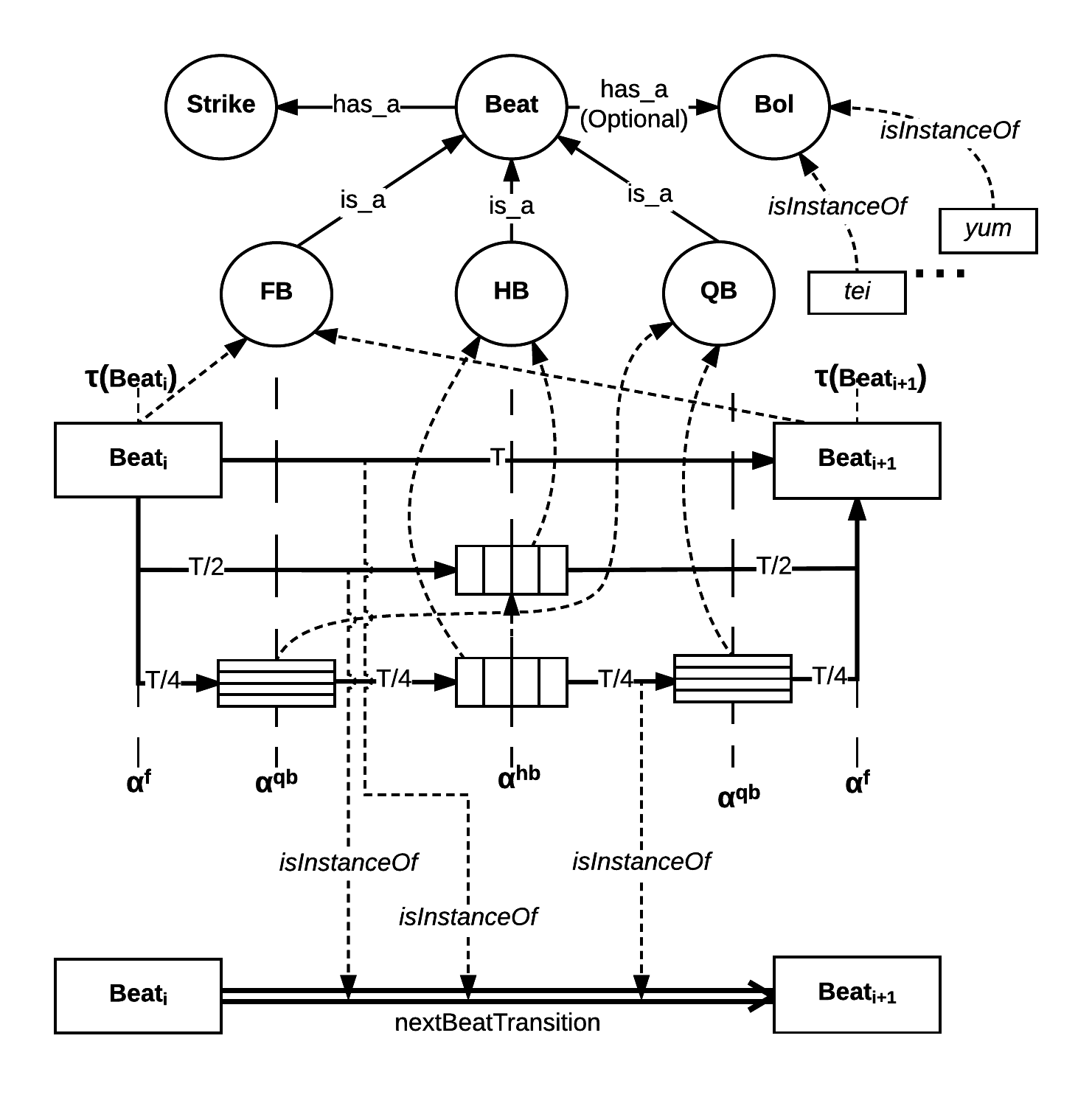
(a) Model of Beats, Bols and Transitions

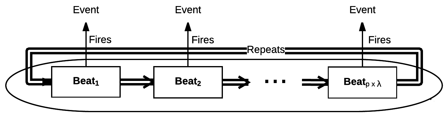
(b) Model of Sollukattu

Figure 1: Event-Driven Ontological Model of Audio

4 Problem Statement & Solution Approach

Let $S$ be the set of Sollukattus. The recording of a Sollukattu $s\in S$ is a discrete-time audio signal $f^{s}(t)$ defined as:

$$f^{s}\equiv f^{s}(t)\equiv\{f^{s}_{0},f^{s}_{1},\cdots,f^{s}_{n-1}\}$$ (1)

where $0\leq t\leq\mathcal{T}$, $\mathcal{T}$ is the duration of the signal, $f^{s}(t)$ is a sequence $\{f^{s}_{i}\}$ of sampled and quantized values, $n=\mathcal{T}\times r$ is the number of samples, and $r$ is the sampling rate.

The sampling and quantization of audio is performed by the recorder at a rate of $r=44100$ sample /sec. $\approx$ 22.7 $\mu s$ = $\delta_{s}$. Hence there is a time-stamp every $\delta_{s}$ sec. available on the audio packets of $f^{s}$. Thus we can mark $f^{s}$ in time with $\delta_{s}$ sec. resolution. However, we deal with coarse-grained events like beats and bols that usually span over 100 ms.

Given an audio signal $f^{s}$, we want to solve for following:

1. Recognize the Sollukattu $s$ of $f^{s}$

2. Mark $f^{s}$ with time-stamps of beats, beat information ($1$, $\frac{1}{2}$ or $\frac{1}{4}$) and associated bols

This, in turn, needs the solution of the following:

1. Recognize and build the sequence of bols in $f^{s}$ (Sec. 6)

   • To detect bols ($\beta$ events), we first segment $f^{s}$ using silence intervals. The MFCC (Mel Frequency Cepstral Coefficients) features of segmented non-silent slices are used with Gaussian Mixture Model (GMM) to classify the bols. The signal $f^{s}$ is then represented in terms of a string signature (called, Signal Signature) comprising the recognized bols.

2. Recognize the Sollukattu $s$ of $f^{s}$ (Sec. 7)

   • To recognize the Sollukattus, we build a dictionary of string signatures of bols (called, Sollukattu Signature) for every Sollukattu. We match the Signal Signature of $f^{s}$ with the Sollukattu Signatures in the dictionary using an edit distance.

3. Estimate the tempo period $T^{s}$ of $s$ from $f^{s}$ (Sec. 8)

   • We estimate the tempo period using two methods:

     1. Working directly with the signal $f^{s}$, we estimate the tempo period by Comb (resonating) filter

     2. We estimate the tempo period from the Longest Common Sub-string (LCS) between Signal Signature and Sollukattu Signature

4. Mark time-stamps and bols of beats in $f^{s}$ (Sec. 9)

   • Beat Positions are a sequence of time-stamps $\tau_{i},i\geq 0$ on $f^{s}$. For tempo period $T^{s}$ of $s$, if there is a $1$-beat ($\alpha^{f}$ event) at $\tau_{i}$, we have $\tau_{i+1}-\tau_{i}\approx T^{s},\forall i$. For a $\frac{1}{2}$-beat ($\alpha^{h}$ event), $\tau_{i+1}-\tau_{i}\approx T^{s}/2$. In [13] we detect beats using detection of onsets in $f^{s}$ and subsequent refinement of the set of detected onsets. This, however, works only for $1$-beats.

   • We use the information of detected beats, detected bols and estimated tempo period to design an algorithm that traverses on $f^{s}$ and marks various events, time-stamps and bols on the signal by exploiting the structural properties of a Sollukattu.

5 Data Set & Annotation

No data set for Sollukattus are available for training and testing purposes of the research. Hence, we had to create a data set by recording performances and then annotating them with the help of expert Bharatanatyam dancers. A part of the data set (SR1) has been published in Audio Data (Sollukattu) [12] for reference and use by researchers.

5.1 Data Set

We record 6 sets (Tab. 2) of 23 Sollukattus using a Zoom H2N Portable Handy Recorder. The first of the sets (SR1) was recorded for only a single bar (cycle) while others are done for 4 bars. Also, in SR1 and SR2, few Sollukattus are recorded multiple times. 162 Sollukattu files corresponding to recording sets SR1–SR6 (Tab. 2) have been recorded and subsequently annotated as follows.

Table 2: Sollukattu Data Set as recorded

Recording	Beater	# of	# of	# of
Set #	#	Sollukattus	Cycles	Recordings
SR1	Beater 1	23	1	30
SR2	Beater 1	23	4	40
SR3	Beater 1	23	4	23
SR4	Beater 1	23	4	23
SR5	Beater 2	23	4	23
SR6	Beater 3	23	4	23
Total				162
$\bullet$ In SR1 and SR2, a few Sollukattus are recorded multiple times

5.2 Annotation

Annotation of a Sollukattu involves the following:

1. Identification the beats and marking them on the signal. Every beat should be marked with its time-stamp as a $1$-, $\frac{1}{2}$-, $\frac{1}{4}$-, or stick beat.

2. Identification the bols and their associations with beats.

3. Marking parts of the signal that are silent.

4. Estimation of the tempo period.

5. Marking of the bars and determination of the number of beats in a bar.

6. Documentation of the annotations in Excel.

Typical annotations are illustrated in Tab. 3 and Fig. 2. We often write the bols of a Sollukattu as a sequence, grouping the bols of the same tempo period with [] brackets. Hence, for the Tatta C Sollukattu (Tab. 3), the bol sequence is:

$[tei\ ya][tei\ ya][tei\ ya][tei][tei\ ya][tei\ ya][tei\ ya][tei]$.

Table 3: Annotations of Tatta C Sollukattu (Fig. 2)

Event	Time	B	HB	Event	Time	B	HB
$\alpha^{fb}_{1}$(tei)	6.57			$\alpha^{fb}_{5}$(tei)	13.03	1.66
$\alpha^{hb}_{1}$(ya)	7.40		0.83	$\alpha^{hb}_{5}$(ya)	13.82		0.79
$\alpha^{fb}_{2}$(tei)	8.19	1.62		$\alpha^{fb}_{6}$(tei)	14.63	1.60
$\alpha^{hb}_{2}$(ya)	8.96		0.77	$\alpha^{hb}_{6}$(ya)	15.44		0.81
$\alpha^{fb}_{3}$(tei)	9.75	1.56		$\alpha^{fb}_{7}$(tei)	16.18	1.55
$\alpha^{hb}_{3}$(ya)	10.57		0.82	$\alpha^{hb}_{7}$(ya)	17.03		0.85
$\alpha^{fb}_{4}$(tei)	11.37	1.62		$\alpha^{fb}_{8}$(tei)	17.81	1.63

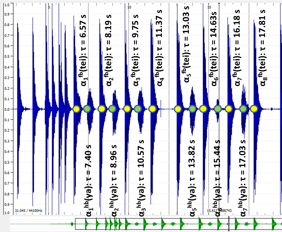
$\bullet$ No. of bars = 2, $\lambda$ = 8 and $T=1.56$ sec. $1$-beats ($\alpha^{fb}$, yellow) and $\frac{1}{2}$-beats ($\alpha^{hb}$, green) are highlighted with bols and time-stamps (Tab. 3).

Figure 2: Annotations of beats and bols for Tatta C Sollukattu

6 Bol Recognition

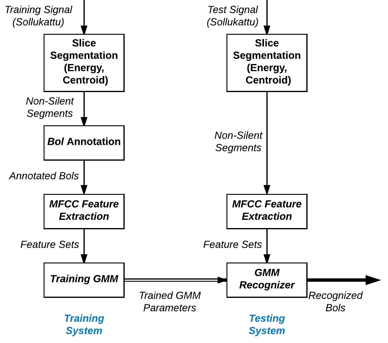
Figure 3: Overview of the Bol Recognition System

The bol recognition system is shown in Fig. 3. In order to train the system, we manually segment the audio signal of every Sollukattu by removing the silence parts (during annotation). This step generates a number of segmented signals of bols and stick-beats. We collect the segments from all Sollukattu signals in the training set and annotate every segment with the bol class. MFCC features are extracted for the bol classes and a GMM classifier is trained.

For testing, we segment the test Sollukattu audio signal (Sec. 6.1), extract MFCC features for every segment, and then recognize every bol using a GMM. Finally, we build a sequence of recognized bols into a signature (Sec. 6.2).

6.1 Segmentation of Audio Signal into Bol Segments

To segment $f^{s}\equiv f^{s}(t)$ into individual bol signals, we detect the silence periods in $f^{s}$ (having value very close to zero) and segment it into a sequence of non-silent slices. A bol (or stick-beat) can only be a non-silent slice of signal. A non-silent slice $\hat{f}^{s}_{i}(t)$ is non-zero in the interval $\tau(\hat{f}^{s}_{i}(t))=[\tau_{s_{i}},\tau_{e_{i}}]$ and is (almost) zero elsewhere. It is defined as:

$\hat{f}^{s}_{i}(t)$	=	$0$,	$0\leq t<\tau_{s_{i}}$
	=	$f^{s}(t)$,	$\tau_{s_{i}}\leq t\leq\tau_{e_{i}}$
	=	$0$,	$\tau_{e_{i}}<t\leq\mathcal{T}$

The signal $f^{s}$, approximated in terms of non-silent slices, is:

$$f^{s}(t)\approx\sum_{i=0}^{k^{s}-1}\hat{f}^{s}_{i}(t)$$ (2)

where $\tau(\hat{f}^{s}_{i}(t))=[\tau_{s_{i}},\tau_{e_{i}}]$, $\forall i,0\leq i<k^{s}-1$, $k^{s}$ is the number of non-silent slices in $f^{s}(t)$, and $0\leq\tau_{s_{i}}<\tau_{e_{i}}<\tau_{s_{i+1}}<\tau_{e_{i+1}}\leq\mathcal{T}$. That is, the non-zero parts of the non-silent slices are non-overlapping. Typically, $k^{s}\gg\lambda^{s}$, number of $1$-beats in a bar of Sollukattu $s$. Hence, the signal has lot more beats or events than a bar of a Sollukattu $s$. Ignoring the silence periods, $f^{s}(t)$ can be expressed by a sequence of slices as:

$$f^{s}(t)\approx\ <\hat{f}^{s}_{i}(t)\ |\ 0\leq i<k^{s}-1>$$ (3)

Every $\hat{f}^{s}_{i}(t)$ represents a bol or stick-beat, that is, $\alpha^{fb}$, $\alpha^{hb}$, or $\alpha^{fn}$ events. To convert $f^{s}(t)$ into the sequence of non-silent slices as above, we use the signal energy and the spectral centroid ([7]) of the audio signal for silence removal and segmentation because the energy of the mixed sound (voice and instrumental) is expected to be larger than the energy of the silent segments.

6.1.1 Segmentation by Silence Detection

We divide the signal $f^{s}(t)$ into overlapping short-term frames, each having a time window $win=0.090$ sec., to compute the silence / non-silence periods. The overlap is taken as $step=0.010$ sec. Thus the $i^{th}$ frame has $N=win*\delta_{s}$ samples given by $x_{i}(n),n=1,...,N$ where $\delta_{s}=44100$ sec^-1 is the sampling rate. Signal energy ($E_{i}$) and spectral centroid ($C_{i}$) features are then calculated for every frame as (1) Signal Energy, $E_{i}=\sum_{n=1}^{N}x^{2}_{i}(n)/N$, and (2) Spectral Centroid, $C_{i}=(\sum_{n=1}^{N}(n+1)X_{i}(n))/(\sum_{n=1}^{N}X_{i}(n))$, where $X_{i}(n)$, $n=1,...,N$ are the DFT coefficients of samples of the $i^{th}$ frame.

The sequence of frames are now converted to sequence of feature values. We threshold based on feature values to remove the silence parts in the audio signal. The thresholds are computed in 3 steps: (1) Compute the histogram of the values in the feature sequence, (2) Detect the local maxima of the histograms, and (3) Let $M_{1}$ and $M_{2}$ be the positions of the first and second local maxima respectively. The threshold value is computed as $T=(W*M_{1}+M_{2})/(W+1)$ where $W$ is a weight to control the cut-off. This process is performed for both feature sequences, leading to two thresholds: $T_{E}$ (energy) and $T_{C}$ (spectral centroid). For the $i^{th}$ frame, if either $E_{i}<T_{E}$ or $C_{i}<T_{C}$ holds, it is considered a part of the silent segment and marked accordingly. The sequence of the remaining frames form the non-silent segments $\hat{f}^{s}_{i}(t),0\leq i<k^{s}$, each representing a bol or a stick-beat. For every segment $\hat{f}^{s}_{i}(t)$ we also mark the start and the end times $\tau(\hat{f}^{s}_{i}(t))$ from the frames involved in it. In Fig. 4, we illustrate the silence detection for an audio signal.

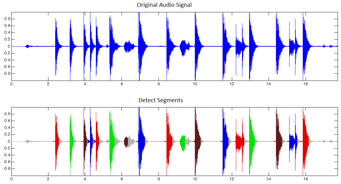
$\bullet$ Silence parts are shown in grey

$\bullet$ Different bol segments are shown in different colors

Figure 4: Silence Removal and Segmentation

We use $W=0$. As a number of Sollukattus have $1$- as well as $\frac{1}{2}$-beats, and as the beating is relatively weak for a $\frac{1}{2}$-beat (though the vocalization is done with the same loudness), the two maxima $M_{1}$ and $M_{2}$ in the histograms correspond to the energy from $1$- and $\frac{1}{2}$-beats respectively. Hence the use of $W>0$ removes part of the $\frac{1}{2}$-beat and weakens the corresponding bol signal.

6.2 Signature of Audio Signal

Let $G$ be a bol recognizer that takes a non-silent signal slice and recognizes the bol:

$$G\ :\ \mathcal{F}\rightarrow\mathcal{B}\cup\{\top\}$$ (4)

where $\mathcal{F}$ is a set of slices $\hat{f}^{s}_{i}(t)$, $0\leq i<k$, $k=|\mathcal{F}|$ is the number of slices in $\mathcal{F}$, $\mathcal{B}$ is the set of bols, $\top$ denotes Undefined / Unrecognized bol arising from stick-beat (or from some failed recognition). So a bol event $\hat{\beta_{i}}$ is recognized as:

$$G(\hat{f}^{s}_{i}(t))=\hat{\beta_{i}}\in\mathcal{B}\cup\{\top\}$$

with bol event time interval $\tau(\hat{\beta_{i}})=\tau(\hat{f}^{s}_{i}(t))=[\tau_{s_{i}},\tau_{e_{i}}]$. We use $\tau(\hat{\beta_{i}})=\tau_{s_{i}}$ or $\tau(\hat{\beta_{i}})=(\tau_{s_{i}}+\tau_{e_{i}})/2$ when we need one instant in place of an interval. Repeatedly using $G$ (Eqn. 4) on every slice of an audio signal $f^{s}(t)$ (Eqn. 3), we get a sequence $\Gamma(f^{s})$ of recognized bols for $f^{s}(t)$ as:

$$\Gamma(f^{s})=<\hat{\beta_{i}}\ |\ 0\leq i<k,\hat{\beta_{i}}\in\mathcal{B}>$$ (5)

$\Gamma(f^{s})$ is called the Signal Signature of $f^{s}(t)$. While building the sequence $\Gamma(f^{s})$ we drop the unrecognized symbol, $\top$. We use $\Gamma(f^{s})$ later for recognizing Sollukattus.

6.3 Bol Recognizer

To build $G$, we first construct a Bol vocabulary comprising all bols in $\mathcal{B}$, use MFCC features to represent every bol and engage Gaussian Mixture Model (GMM) as a recognizer.

6.3.1 Bol Vocabulary

The bol vocabulary, as identified by the experts, is given in Tab. 4. We also denote a class for stick-beats or $\bot$ (no bol) to eliminate $\alpha^{fn}$ segments from the rest. We encode every class with a unique number (Bol Code) in Tab. 4.

Table 4: Bol data from SR1–SR6 data sets for Bol classes

Bol	Bol	Trg.	Test	Bol	Bol	Trg.	Test
Class	Code	Data	Data	Class	Code	Data	Data
a	1	139	34	ka	17	155	38
da	2	93	19	ki	18	193	50
dha	3	100	26	ku	19	48	13
dhat	4	142	35	na	20	383	95
dhi	5	55	16	ri	21	44	9
dhin	6	324	81	ta	22	1212	306
dhit	7	1052	264	tak	23	138	35
ding	8	80	21	tam	24	484	121
e	9	142	35	tan	25	353	89
gadu	10	181	46	tat	26	1825	457
gin	11	93	23	tei	27	4060	1019
ha	12	447	112	tom	28	194	50
hat	13	171	42	tta	29	160	40
hi	14	154	37	ya	30	158	39
jag	15	22	8	yum	31	284	71
jham	16	32	11	Stick/$\bot$	32
				(no bol)	or 99

6.3.2 Features of Bols

Since most segmented audio signals (with the exception of stick-beats) contain utterances, we use MFCC [17] features, common for speech recognition tasks, to represent them. For each of segmented bol signal $\hat{f}^{s}_{i}(t)$ we calculate 13 dimensional MFCC features using the algorithm in [4]. We also concatenate the dynamics features – 13 delta and 13 delta-delta ($1^{st}$- and $2^{nd}$-order frame-to-frame difference) coefficients to get 39 features. Our choice is guided by the experimental results of [21] showing robustness of the extended features to background noise.

6.3.3 GMM Training

For recogniton of bols from MFCC features we use GMM [18]. GMM parameters are estimated from training data using the iterative Expectation-Maximization (EM) algorithm.

As noted in Tab. 4, we have $n_{b}=32$ Bol classes $C=$ $\{C_{1},\cdots,C_{n_{b}}\}$. The GMM is trained using MFCC feature vectors of these classes. The parameters of the GMM for $C_{j}$ are estimated from the training data set. We train the GMM with 80% of the bols from the total sample of each class and save the mean, variance (diagonal covariance) and weight for each vocab class $C_{j}$ as the model for this class. We use $M=15$ Gaussian components based on trials with a subset of data.

6.3.4 Recognition Test

We use remaining 20% data of each class to test the model. Given the Gaussian mixture parameters for each bol class, a test vector $\mathbf{x}$ is assigned to the class $C_{j}$ that maximizes $p(C_{j}|\mathbf{x})$. That is, $p(C_{j}|\mathbf{x})>p(C_{i}|\mathbf{x}),\forall i,1\leq i\leq{n_{b}}$. We assume that each class has equal a priori probability $p(C_{j})=1/{n_{b}}$. Hence, maximizing $p(C_{j}|\mathbf{x})$ is equivalent to maximizing $p(\mathbf{x}|C_{j})$ because: $p(C_{j}|\mathbf{x})=p(\mathbf{x}|C_{j})p(C_{j})=p(\mathbf{x}|C_{j})/{n_{b}}$.

As the occurrences of different bols in the Sollukattus are known, $p(C_{j})$s may be estimated from these distributions provided the distribution of the Sollukattus is known. We do not assume uniform distribution and choose to use $p(C_{j})=1/{n_{b}}$ for simplicity.

6.4 Results & Analysis

The distribution of bols in various classes and their partitions in training and test sets are shown in Tab. 4. We have performed the bol recognition for each of SR1 through SR6 data sets and also by taking all the data sets together. In each data set we use 80% of the data in each class for training and 20% for testing. The results are summarized in Tab. 5. Overall, it was possible to achieve 85.13% accuracy in bol recognition.

The confusion matrix for SR1-SR6 data set is shown in Tab. 6. From the confusion matrix we find that a group of bols ‘ta’, ‘tak’, ‘tam’, ‘tan’ are often mis-classified among themselves. This is due to the strong similarity of their sound.

	ta	tak	tam	tan	tat	tei	tom	tta	Total
ta	32.4	15.4	13.1	0.3	6.9	0.0	0.3	14.1	306
tak	11.4	68.6	2.9	0.0	0.0	0.0	0.0	17.1	35
tam	9.1	0.0	86.0	0.0	0.0	0.8	0.0	0.0	121
tan	15.7	0.0	46.1	37.1	0.0	0.0	0.0	0.0	89
tat	0.4	2.2	0.0	0.0	88.4	0.0	0.7	1.8	457
tei	0.0	0.0	0.0	0.0	0.3	90.9	0.3	0.0	1019
tom	0.0	0.0	0.0	0.0	0.0	4.0	94.0	0.0	50
tta	0.0	5.0	0.0	0.0	0.0	0.0	0.0	95.0	40

Table 5: Results of Bol recognition

Data Set	Recognition	Data Set	Recognition
	Rate (%)		Rate (%)
SR1	85.79	SR4	91.05
SR2	87.27	SR5	84.03
SR3	94.53	SR6	88.06
SR1–SR6	85.13

Table 6: Confusion matrix for Bol recognition

Actual Bol	Predicted Bol
	Bol	Self	Error	Total	Bol	Self	Error	Total
	a	58.8	(17.6, ta)	34	ka	92.1		38
	da	84.2		19	ki	72.0		50
	dha	84.6		26	ku	92.3		13
	dhat	82.9		35	na	61.1	(11.6, tam)	95
	dhi	56.3	(12.5, dhit), (12.5, gin)	16	ri	77.8	(11.1, dha), (11.1, ding)	9
	dhin	87.7		81	ta	32.4	(11.4, ka), (15.4, tak), (13.1, tam), (14.1, tta)	306
	dhit	87.9		264	tak	68.6	(11.4, ta), (17.1, tta)	35
	ding	90.5		21	tam	86.0		121
	e	91.4		35	tan	37.1	(15.7, ta), (46.1, tam)	89
	gadu	100.0		46	tat	88.4		457
	gin	82.6		23	tei	90.9		1019
	ha	88.4		112	tom	94.0		50
	hat	90.5		42	tta	95.0		40
	hi	78.4	(16.2, e)	37	ya	87.2		39
	jag	87.5	(12.5, tat)	8	yum	100.0		71
	jham	54.5	(36.4, jag)	11
	Results for SR1–SR6 data sets (Tab. 2). For test data (Tab. 4), the diagonal entries (in %) of the confusion matrix are shown as ‘Self’. Entries with 10%+ error are shown under ‘Error’. For example, for Bol = a, the diagonal entry is 58.8% and it is mis-classified as ta in 17.6% cases. ‘Total’ shows the number of symbols in the class

Similar cases may also be found of ‘ta’ and ‘tak’ mis-classified as ‘tta’, ‘ta’ as ‘ka’, ‘jham’ as ‘jag’, and so on. To reduce mis-classifications and improve accuracy, we certainly need to improve training. For example, ‘jham’ has only 32 training samples and ends up with 54.5% accuracy. Interestingly, lack of training does not necessarily result in poor accuracy – ‘jag’ attains 87.5% accuracy with only 22 training samples and ‘ta’ ends up with 32.4% in spite of having 1212 training samples. In some cases, however, completely differently sounding bols are also mis-classified like ‘ri’ as ‘dha’. This is due to error in segmentation by silence removal because they occur side-by-side in Tirmana C Sollukattu. It was observed that the following factors influence the accuracy of bol recognition:

• More similar sounding bols degrade performance. Distinctiveness of the sound of a bol helps better recognition.

• More training samples should improve performance.

• The context of a bol may have significant impact on the accuracy (due to the segmentation) – particularly the time gap with the previous and next bols.

Using the Bol recognizer $G$ as above, we construct the Signal Signature $\Gamma(f^{s})$ of the Sollukattu signal $f^{s}$ of $s$ and recognize $s$.

7 Sollukattu Recognition

To recognize Sollukattus we associate a Signature with a Sollukattu. Let us define a Sollukattu Sequence $\Omega(s)$ of $s\in S$ as:

$$\Omega(s) = <\omega_{i}\ |\ \omega_{i}=(\alpha_{i},\beta_{i}),\alpha_{i}\in A,$$

$$\beta_{i}\in\mathcal{B}\cup\{\bot\},0\leq i<n_{e}^{s}>$$

where $A$ is the set of beat events, $i$ denotes serial position of $1$- or $\frac{1}{2}$- or $\frac{1}{4}$-beat in $s$, and $n_{e}^{s}$ is the number of beat ($\alpha$) events in $s$. If a beat does not have a bol (stick-beat), $\bot$ is marked for the $\beta$ event as a placeholder.

By now we know part of the $\alpha$ events ($1$-beats, $\alpha^{f}$ from beat detection in [13]), all the $\beta$ events, and Signal Signature $\Gamma(f^{\hat{s}})$ (Sec. 6.2) of $f^{\hat{s}}$, where $\hat{s}$ is the placeholder for the unknown Sollukattu. We also know the time-stamps of the events, that is, $\tau(\alpha)$ and $\tau(\beta)$. So we next define Signatures of Sollukattus.

7.1 Signature of Sollukattu

The Signature $\zeta(s)$ of a Sollukattu $s\in S$ is defined as:

$$\zeta(s)=<\beta_{i}\ |\ \beta_{i}\in\mathcal{B},0\leq i<\mathcal{K}^{s}>$$ (6)

by first dropping the $\alpha$ part of every $\omega$ in a Sollukattu Sequence $\Omega(s)$ and then dropping the stick-beats ($\bot$). The signature, therefore, is a pure syntactic representation (string over set of bols $\mathcal{B}$) of a Sollukattu that preserves the sequencing but ignores the temporal arrangement. The length of the signature $|\zeta(s)|=\mathcal{K}^{s}$ denotes the number of bols ($\beta$ events) in a bar of Sollukattu $s$. For example, for Natta Sollukattu, the bols are as (in the notation of Sec. 5.2):

$[tei\ yum][tat\ tat][tei\ yum][ta][tei\ yum][tat\ tat][tei\ yum][ta]$

Ignoring the $\alpha$ part ($1$- or $\frac{1}{2}$-beat information), we get:

$\zeta(Natta)=tei-yum-tat-tat-tei-yum-ta-tei-yum-tat-tat-tei-yum-ta$.

Similarly, for Tirmana A, the bols are as:

$[ta][hat\ ta][jham][ta\ ri][ta][B][jham][tari][jag][ta\ ri][tei][B]$, where $[B]$ is a beat without bol. After dropping the $\alpha$, we get:

$ta\ hat\ ta\ jham\ ta\ ri\ ta\ \bot\ jham\ tari\ jag\ ta\ ri\ tei\ \bot$

Hence, after skipping the stick-beats, we get:

$\zeta(Tirmana\ A)=ta-hat-ta-jham-ta-ri-ta-jham-tari-jag-ta-ri-tei$

All Sollukattus, with the exception of Tatta B and Tatta E, have distinct signatures. Hence we build a dictionary $\mathcal{D}$ of Sollukattu Signatures. Once we recognize the bols in an audio stream $f^{s}$ and form its Signal Signature $\Gamma(f^{s})$ as the sequence of recognized bols, we attempt to recognize the corresponding Sollukattu by matching it against the signatures in $\mathcal{D}$.

7.2 Sollukattu Recognizer

Signature of the signal $\Gamma(f^{\hat{s}})$ and signatures of Sollukattus $\zeta(s)$s are both strings defined over the same alphabet $\mathcal{B}$. However, they have different lengths. $|\Gamma(f^{\hat{s}})|=k^{\hat{s}}$ and $|\zeta(s)|=\mathcal{K}^{s}$, $s\in S$. Typically, the signal contains multiple cycles (bars) of the Sollukattu $\hat{s}$. Hence, often $k^{\hat{s}}\gg\mathcal{K}^{s}$. So every $\zeta(s)$ is repeated $\lceil k^{\hat{s}}/\mathcal{K}^{s}\rceil$ number of times and then $(\mathcal{K}^{s}-(k^{\hat{s}}\mod\mathcal{K}^{s}))$ symbols are truncated from the end to bring both signatures to the same length $k^{\hat{s}}$. $\zeta(s)$, so extended, is represented as $\zeta^{*}(s)$.

To recognize the Sollukattu, we use approximate string matching. For this we encode the bols in the strings using the encoding scheme given in Tab. 4. We then compute the Best Match between $\Gamma(f^{\hat{s}})$ and $\zeta^{*}(s)$, $s\in S$ using Levenshtein (Edit) Distance, $d_{Lev}$.

7.2.1 Matching by Levenshtein (Edit) Distance

For two strings $a$ and $b$, $d_{Lev}(a,b)$ is defined as $d_{Lev}(a,b:|a|,|b|)$ where, $d_{Lev}(a,b:i,j)$ is the distance between the first $i$ characters of $a$ and the first $j$ characters of $b$ given by:

$d_{Lev}(a,b:i,j)$
	= $max(i,j)$, if $min(i,j)=0$
	= $min\{d_{Lev}(a,b:i-1,j)+1$, otherwise
	$\quad\quad\quad\;d_{Lev}(a,b:i,j-1)+1$,
	$\quad\quad\quad\;d_{Lev}(a,b:i-1,j-1)+cost(a_{i},b_{j})\}$

where $cost(a_{i},b_{j})=0$ if $a_{i}=b_{j}$, and $=1$, otherwise. $d_{Lev}$ is computed assuming unit cost of insert, delete, and replace operations. We compute $d_{Lev}(\Gamma,\zeta^{*}(s))$, $\forall s\in S$ and find the minima. The Sollukattu of $\Gamma(f)$ is recognized as $s$ if

$$d_{Lev}(\Gamma,\zeta(s))=\min_{s^{\prime}\in S}d_{Lev}(\Gamma,\zeta^{*}(s^{\prime}))$$

7.3 Results & Analysis

The distance matrix for SR2 data set (Tab. 2) having 40 Sollukattu audio files is shown in Tab. 7.

Table 7: Distance matrix of edit distance for SR2

Test	Self	Next min. distance or
Sollukattu file	Dist.	all min. distances below the correct match
Joining A	5	Tattal, 17
Joining B	0	Joining C, 11
Joining C	1	Tatta G, 14
Kartari	50	Tirmana B, 160
Utsanga	25	Nattal A, 21; Tatta F, 21; Nattal B, 22; Natta, 24; Tatta B / E, 25; Joining A, 25
Mandi 1	70	Natta, 292
Sarikkal 1	64	Natta, 316; Tatta F, 316
Sarikkal 2	29	Tirmana B, 72
Kuditta Mettu 1	0	Sarika, 32
Kuditta Mettu 2	2	Sarika, 18
Kuditta Mettu 3	0	Sarika, 64
Kuditta Nattal A1	7	Nattal B, 21
Kuditta Nattal A2	29	Nattal B, 35
Kuditta Nattal B1	5	Nattal A, 21
Kuditta Nattal B2	2	Nattal A, 18
Kuditta Tattal 1	3	Paikkal, 120; TTD, 120
Kuditta Tattal 2	4	TTD, 221
Kuditta Tattal 3	0	Paikkal, 80; Pakka, 80; TTD, 80
Kuditta Tattal 4	2	Paikkal, 41; TTD, 41
Natta 1	2	Tatta F, 23
Natta 2	33	Tatta F, 29
Natta 3	11	Tatta F, 99
Paikkal 1	27	Tatta F, 103
Pakka 1	4	Tatta F, 61
Pakka 2	4	Tatta F, 120
Pakka 43	4	Tatta F, 32; Tatta G, 32; TTD, 32
Sarika 1	5	Nattal A, 63
Sarika 2	7	Nattal A, 13
Tatta A	26	Tatta C, 27
Tatta B	0	Tatta F, 9
Tatta C	2	Tatta A, 12
Tatta D	0	Tatta B / E, 11
Tatta E	5	Tatta A, 20; Tatta F, 20
Tatta F	1	Tatta B / E, 22
Tatta G	1	KUMS, 19
Tei Tei Dhatta 1	33	Pakka, 58
Tei Tei Dhatta 2	20	Pakka, 36
Tirmana A	25	Tattal, 44; TTD, 44
Tirmana B	24	Tirmana C, 135
Tirmana C	111	Tirmana B, 201
$\bullet$ KUMS is Kartati Utsanga Mandi Sarikkal, Mettu is Kuditta Mettu, Nattal is Kuditta Nattal, Tattal is Kuditta Tattal and Tei Tei Dhatta is TTD
$\bullet$ Self Distance is the distance with the correct entry for the input Sollukattu in the dictionary. If it is the minimum (correct match), we show the next minimum for an estimate of discrimination of edit distance. If it is not the minimum (wrong match), we show all distances that are smaller than it.
$\bullet$ Some Sollukattus have multiple recorded files as shown with serial numbers. 40 files for 23 Sollukattus in SR2
$\bullet$ Two Sollukattus (shown in red, bold) are wrongly classified. Hence the accuracy is $(40-2)/40=95\%$ (Tab. 9)
$\bullet$ Tatta B and Tatta E have the same signature (differ only in stick-beats)

We see that recognition fails for two Sollukattus:

• Utsanga_HB2.wav (KUMS) is mis-classified as Kuditta Nattal A. It may noted (Tab. 8(a)) that the key bol ‘tan’ of KUMS is repeatedly mis-classified, often as ‘tam’. The other key bol ‘gadu’ is often missed. In contrast, ‘tei’ is getting recognized which does not exist in this Sollukattu. This results in a stronger similarity with and classification to Kuditta Nattal A.

• Natta_35678_HB2.wav (Natta) is mis-classified as Tatta F. The bol ‘yum’ of Natta is totally missing making it very close to the signature of Tatta F (Tab. 8(b)).

Table 8: Error cases in Sollukattu recognition

$\Gamma($Utsanga_HB2.wav$)$
hi	tam	gadu	tat	tat	na	tam	tat	tat	tei	ta	tam	tat	tei	$\cdots$
14	24	10	26	26	20	24	26	26	27	22	24	26	27	$\cdots$
$\zeta($KUMS$)$: [tan gadu] [tat tat] [dhin na] [tan gadu] [tat tat] [dhin na]
tan	gadu	tat	tat	dhin	na	tan	gadu	tat	tat	dhin	na	tan	gadu	$\cdots$
25	10	26	26	06	20	25	10	26	26	06	20	25	10	$\cdots$
$\zeta($Kuditta Nattal A$)$: [tat] [tei] [tam] [B] [dhit] [tei] [tam] [B]
tat	tei	tam	dhit	tei	tam	tat	tei	tam	dhit	tei	tam	tat	tei	$\cdots$
26	27	24	07	27	24	26	27	24	07	27	24	26	27	$\cdots$
(a)
$\Gamma($Natta_35678_HB2.wav$)$
tei	tat	tat	tei	ta	tei	tat	tei	ta	tei	tat	tat	tei	ta	$\cdots$
27	26	26	27	22	27	26	27	22	27	26	26	27	22	$\cdots$
$\zeta($Natta$)$: [tei yum] [tat tat] [tei yum] [ta] [tei yum] [tat tat] [tei yum] [ta]
tei	yum	tat	tat	tei	yum	ta	tei	yum	tat	tat	tei	yum	ta	$\cdots$
27	31	26	26	27	31	22	27	31	26	26	27	31	22	$\cdots$
$\zeta($Tatta F$)$: [tei] [tei] [tat] [tat] [tei] [tei] [tam] [B]
tei	tei	tat	tat	tei	tei	tam	tei	tei	tat	tat	tei	tei	tam	$\cdots$
27	27	26	26	27	27	24	27	27	26	26	27	27	24	$\cdots$
(b)

Of the total 162 Sollukattu recordings, 8 were partially corrupted and could not be used. Of the remaining 154 files, 7 were mis-classified. So we achieve 95.45% accuracy in Sollukattu recognition (Tab. 9). Next we estimate the tempo period.

Table 9: Results of Sollukattu recognition

Data	No. of	No. Correctly	% Rate of	Mis-classification	Remarks
Set	Audio Files	Recognized	Recognition	File: Actual Sollukattu $\rightarrow$ Predicted Sollukattu
SR1	30	29	96.67	Tirmana_1_HB1.wav: Tirmana A $\rightarrow$ Joining A
SR2	40	38	95.00	Natta_35678_HB2.wav: Natta $\rightarrow$ Tatta F	Edit distance matrix shown in Tab. 7
				Utsanga_HB2.wav: KUMS $\rightarrow$ Kuditta Nattal A
SR3	20	19	95.00	Tatta_4_HB4.wav: Tatta C $\rightarrow$ Tatta D	3 files were partially corrupted & skipped:
					Joining A, Kuditta Nattal A, KUMS
SR4	22	21	95.45	Tatta_4_HB4.wav: Tatta C $\rightarrow$ Tatta D	1 file was partially corrupted & skipped:
					Tatta B
SR5	22	20	90.91	Tatta_12_MD1.wav: Tatta A $\rightarrow$ Tatta D	1 file was partially corrupted & skipped:
				Tatta_4_MD1.wav: Tatta C $\rightarrow$ Tatta A	Joining C
SR6	20	20	100.00		3 files were partially corrupted & skipped:
					Kuditta Tattal, KUMS, Tatta A
Total	154	147	95.45
$\bullet$ Data Sets from Tab. 2. KUMS is Kartati Utsanga Mandi Sarikkal

8 Tempo Period Estimation

In an earlier paper [13] we reported the detection of $1$-beats with their time-stamps. This approach can be used to compute the tempo period from the difference of time-stamps of two consecutive $1$-beats. This difference should be identical for two consecutive $1$-beats and be the same as $T^{s}$. An estimator may also be designed based on the time-stamps of detected bols. However, these strategies do not work well due to human errors in creating the signal and due to limitations of the detection algorithms. We outline the issues below:

1. The difference of time-stamp of two consecutive $1$-beats vary (substantially at times) due to the human error in beating the stick or uttering the bols or both. Situation worsens when the Sollukattu has $\frac{1}{2}$- and $\frac{1}{4}$-beats.

2. The segmentation of $f^{s}(t)$ by silence (Sec. 6.1) may have some errors. This propagates to the estimated time-stamp of the detected bol.

3. Many Sollukattus have $\frac{1}{2}$-beats, some even have $\frac{1}{4}$-beats. Due to the error in bol recognition, at times it may not be possible to correctly identify if a slice (and its time-stamp) corresponds to a $1$-beat or a $\frac{1}{2}$-beat. This may cause errors in time gaps.

We explore two approaches for estimation of tempo period:

• Estimation from the audio signal $f^{s}$ using Resonating / Comb Filter

  • This operates at the low level, working directly with the signal

• Estimation using Longest Common Sub-string (LCS) between Signal signature and Sollukattu Signature

  • This operates at the high level, exploiting the structural information extracted so far

8.1 Estimation using Comb Filter

A comb filter is often used for tempo estimation and beat tracking in music signal processing ([20]). If a piece of music can be characterized as consisting of musical events which are often on the beat, then we may expect that signal processing methods such as comb filtering and auto-correlation to succeed in locating the beats.

To estimate the tempo period, we use the method in [20].

1. Frequency Filter-bank: First the audio signal $f^{s}$ is passed through a bank of 3 filters corresponding to 3 typical bands; namely, vocal (0-900Hz), instrumental beating (900-2600Hz) and harmonics (2600-22100Hz). Output of each filter, in time domain, is processed through the following steps.

2. Envelop Extractor: The signal $f^{s}$ has a range of frequencies in every band. However, we are interested only in the overall trend (the slow periodicity of the signal devoid of the fine changes at every frequency). And we expect this trend to be similar in every band. So we need to compute the envelop of the signal where only sudden changes in the signal can strongly manifest. Naturally, we need to filter the frequency-banded signals using low-pass filters. Hence, we first full-wave rectify the signals to reduce high-frequency content and restrict to the positive half of the envelope. We then convolve each signal by the right half of a Hanning Window for low-pass filtering. Much of this computation is performed in the frequency domain for ease of implementation and computational efficiency.

3. Differentiator: The envelop signal is next differentiated in time domain to manifest sudden changes in its amplitude.

4. Half-wave Rectifier: The differentiated signal is half-wave rectified to enhance the changes. Now the signal resembles a sequence of (imperfect) impulses. The temporal periodicity in these impulses indicate the tempo period. We intend to estimate that by combing.

5. Resonant Filter-bank: We construct a set of equi-spaced impulse trains having adjustable periodicity (spacing) for impulses. We expect that the periodicity of one of these impulse trains will match the periodicity of our sequence of impulses. So if we convolve the impulse train with our sequence, the resulting energy will maximize (resonate) when their periods match. We perform this in frequency domain with periodicity varying from 33 bpm (bpm_min = 33 $\approx$ 1.8 sec.) to 75 bpm (bpm_max = 75 $\approx$ 0.8 sec.) in unit steps. We convolve to compute the energy in each band. The bpm $p$ corresponding to maximum sum of energy is taken to be the fundamental bpm of the audio signal. The tempo period is then computed as 60/$p$ sec.

The results of tempo period estimation by this methods are shown in Tab. 10. We analyze in Sec. 8.3.

8.2 Estimation using LCS between Signatures

After recognizing the Sollukattu $s$ for test signal $f^{s}$, we know the following:

• The Signal Signature $\Gamma(f^{s})$ has detected sequence of bols with time-stamps. Some bols in this sequence may be wrong, time-stamps may be erroneous, and bols may be at $1$-beat or $\frac{1}{2}$-beat positions (and we do not know which is at $1$-beat and which is at $\frac{1}{2}$-beat). So we cannot compute the tempo period ($1$-beat to $1$-beat gap) directly from such a signature.

• The Sollukattu Signature $\zeta(s)$ having correct sequence of bols. We also know if these bols are at $1$- or $\frac{1}{2}$-beats positions. However, we do not know their time-stamps.

If the recognition of bols in $\Gamma(f^{s})$ were all correct, we could just match it up with $\zeta^{*}(s)$ (Sec. 7.2) symbol by symbol to know the bols at $1$-beat and then use their time-stamps to get the tempo period. This is not possible because there will be wrong bols in $\Gamma(f^{s})$. However, if we assume that most bols are correctly recognized in $\Gamma(f^{s})$ (which is often the case), then we can expect long sub-strings of bols that are correct and match them against $\zeta(s)$. The longer the sub-string, better will be the quality of the match. Hence we look for longest common sub-string $\mathcal{L}(\Gamma,\zeta)$ between $\Gamma(f^{s})$ and $\zeta(s)$. It is expected that such a sequence will be long enough to contain multiple $1$-beats ($\alpha^{f}_{i}$, $0\leq i<|\mathcal{L}(\Gamma,\zeta)|$) that can now be correctly known for their time-stamps. Thus one can have a number of estimates ($T_{est}^{i}=\tau(\alpha^{f}_{i+1})-\tau(\alpha^{f}_{i})$, $0<i\leq|\mathcal{L}(\Gamma,\zeta)|$) for the tempo period and choose their median as a robust estimator. Formally:

8.2.1 Longest Common Sub-strings (LCS)

Let $a$ be a string of length $|a|=n$. $a_{i..j}$, $i\leq j$ is a sub-string of $a$ containing $i^{th}$ to $j^{th}$ symbols. For two strings $a$ ($|a|=n$) and $b$ ($|b|=m$) over the same alphabet, the length of the longest common suffix for all pairs of prefixes of the strings are defined by the following recursion:

$LCS_{Suff}(a_{1..n},b_{1..m})$
	= $LCS_{Suff}(a_{1..n-1},b_{1..m-1})+1$, if $a_{n}=b_{m}$
	= 0, otherwise

$LCS_{Suff}$ can be computed efficiently using dynamic programming. The longest suffix strings may be constructed by tracing back on the updates of the DP tableau. The length of the longest common sub-strings (LCS) of $a$ and $b$ is the maximum of the lengths of the longest common suffixes:

$$LCS(a_{1..n},b_{1..m})=\max_{\begin{subarray}{c}1\leq i\leq n,1\leq j\leq m\end{subarray}}LCS_{Suff}(a_{1\cdots i},b_{1\cdots j})$$

There may be multiple suffixes having this maximum value. All of them are longest common sub-strings of $a$ and $b$.

Consider Joining B. Given $\zeta(Joining\ B)$:

dhit	dhit	tei	dhit	dhit	tei	dhit	dhit	tei	dhit	dhit	tei
7	7	27	7	7	27	7	7	27	7	7	27
B	HB	B	B	HB	B	B	HB	B	B	HB	B

and $\Gamma(f^{Joining\ B})$ for a sample audio:

[7–7–27–7–7–27–7–7–27–7–7–27–7–7–27–7–7–27–7–7–27–7–7–27]

the LCS and time-stamps are obtained as:

LCS, $\mathcal{L}(\Gamma,\zeta)$	07	07	27	07	07	27
$\alpha$	B	HB	B	B	HB	B
$\tau(\alpha)$ in sec.	1.04	1.97	2.90	4.58	5.38	6.19
$T_{est}$ in sec.	1.86		1.68	1.61		1.53
LCS, $\mathcal{L}(\Gamma,\zeta)$	07	07	27	07	07	27
$\alpha$	B	HB	B	B	HB	B
$\tau(\alpha)$ in sec.	7.72	8.46	9.23	10.62	11.37	12.11
$T_{est}$ in sec.	1.51		1.39	1.49

Hence, the estimated tempo period is the median of row $T_{est}$, that is, 1.53 sec. The annotated time for this is 1.52 sec.

8.3 Results & Analysis

8.3.1 By Comb filter

The estimation of tempo period by Comb filter has been tested with SR1 data set (Tab. 2). The result is given in Tab. 10. All tempo periods have been accurately estimated with the sole exception of Joining B Sollukattu. So we could achieve 96.67% accuracy in estimation of tempo period by Comb filter.

Table 10: Results of tempo estimation from Bols

		Estimation Methods
		Comb Filter		LCS
Sollukattu	Actual	Est.	Abs.	Est.	Abs.
Name	Tempo	Tempo	Error	Tempo	Error
Joining A	1.18	1.15	0.03	1.22	0.04
Joining B	1.52	0.80	0.72	1.53	0.01
Joining C	1.17	1.15	0.02	1.17	0.00
Kartari Utsanga	1.07	1.02	0.05	1.11	0.04
Mandi Sarikkal	1.00	1.09	0.09	1.05	0.05
Kuditta Mettu 1	1.16	1.15	0.01	1.16	0.00
Kuditta Mettu 2	1.16	1.07	0.09	1.08	0.08
Kuditta Nattal A	0.99	0.98	0.01	1.05	0.06
Kuditta Nattal B	1.30	1.30	0.00	1.31	0.01
Kuditta Tattal 1	1.21	1.20	0.01	1.22	0.01
Kuditta Tattal 2	1.21	1.15	0.06	1.13	0.08
Kuditta Tattal 3	1.21	1.09	0.12	1.10	0.11
Kuditta Tattal 4	1.21	1.18	0.03	1.15	0.06
Natta 1	1.39	1.40	0.01	1.38	0.01
Natta 2	1.39	1.36	0.03	1.36	0.03
Paikkal	1.58	1.58	0.00	1.55	0.03
Pakka 1	1.21	1.20	0.01	1.21	0.00
Pakka 2	1.21	1.15	0.06	1.14	0.07
Sarika	0.93	0.92	0.01	0.90	0.03
Tatta A	1.51	1.50	0.01	1.52	0.01
Tatta B	1.36	1.33	0.03	1.35	0.01
Tatta C	1.56	1.58	0.02	1.55	0.01
Tatta D	1.35	1.36	0.01	1.34	0.01
Tatta E	1.17	1.18	0.01	1.20	0.03
Tatta F	1.21	1.20	0.01	1.25	0.04
Tatta G	1.41	1.30	0.11	1.32	0.09
Tei Tei Dhatta	1.41	1.40	0.01	1.41	0.00
Tirmana A	1.23	1.22	0.01	fail	fail
Tirmana B	1.22	1.18	0.04	1.21	0.01
Tirmana C	1.46	1.36	0.10	1.35	0.11
$\bullet$ Results for SR1 data set (Tab. 2). Multiple samples from a Sollukattu are serially numbered
$\bullet$ Tempo period for 29 out of 30 sample signals are correctly estimated by each method. Errors in estimation are highlighted

The tempo period of Joining B has been estimated as 0.72 sec. while it actually is 1.52 sec., that is, almost the double. Checking the signal (Fig. 5) we find that in this case the $\frac{1}{2}$-beats have same energy as the $1$-beat. Hence, there are equal peaks at $\frac{1}{2}$-beats as well and the fundamental bpm has been computed based on the number of $\frac{1}{2}$- and $1$-beats instead of just the $1$-beats. Such errors, however, may be easily corrected once the Sollukattu has been recognized and $\frac{1}{2}$-beats are known.

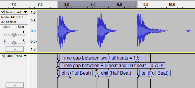
Figure 5: Signal of Joining B Sollukattu

8.3.2 By LCS

The estimation of tempo period by LCS has also been tested with SR1 data set (Tab. 2). The result is given in Tab. 10. We find that this method is as accurate as the Comb filter based method and we achieve 96.67% accuracy in estimation of tempo period by LCS.

This algorithm, however, fails for Tirmana A. Due to error in bol recognition, the LCS in this case contains only one $1$-beat. Hence the tempo period cannot be computed.

We use the tempo period detected by LCS method for beat marking. Comb filter based tempo period is used when the LCS based method fails.

9 Beat Marking

Now we are ready to mark the beats ($\alpha$ events) on the audio signal $f^{s}(t)$. This would involve the following:

1. Mark time-stamps on $f^{s}(t)$ that are beats.

2. Annotate every such marking as a $1$-beat ($\alpha^{fb}$), $\frac{1}{2}$-beat ($\alpha^{hb}$), or stick-beat ($\alpha^{fn}$). Note that $\frac{1}{4}$-beats ($\alpha^{qb}$) are not considered.

3. For a $1$- ($\alpha^{fb}$) or a $\frac{1}{2}$-beat ($\alpha^{hb}$), annotate the bol symbol.

With this it would be possible to automatically generate audio annotations as shown in Fig. 2.

For this task we use the following information as extracted:

1. Detected Beats: Array ($DB$) of $1$-beats extracted using onset (as in [13]). Each beat has a time-stamp.

2. Signal Signature: Array ($SS$) of bols extracted through bol recognition (Sec. 6.2, 6.3). Each bol has an associated time-interval (from the non-silent slice).

3. Estimated tempo period $T$ (Sec. 8).

In addition, we classify non-silent slices $\hat{f}^{s}_{i}(t)$, $0\leq i<k^{s}-1$ (Eqn. 3) of the bols as having $high$ or $low$ energy. We calculate energy of every slice as in Sec. 6.1.1 and cluster the values by $k$-means clustering with $k=2$. The energy class $\epsilon$ ($high$ or $low$) is then marked on Signal Signature array $SS$.

To mark and annotate $f^{s}(t)$, we note the following structural properties of a Sollukattu:

1. The time gap between consecutive $1$-beats should approximately match the tempo period $T$.

   • We use a wider period $wide(T)=[T-0.25,T+0.4]$ for a beat-to-beat gap.

2. A bol always occurs with a beat. Hence its offset from the previous $1$-beat should

   • approximately match the tempo period ($wide(T)$) if it occurs with a $1$-beat, or

   • be less than the tempo period if it occurs with a $\frac{1}{2}$-beat

3. A $1$-beat with bol has higher energy than a stick-beat.

   • This may help filter wrongly detected bols (from stick-beats) from being marked as a $1$-beat.

4. There should be a $1$-beat at the approximate periodicity of the tempo period.

   • If there is a long gap between $1$-beats, say, more than $long\_gap(T)=2*T-0.25$; a beat must have been missed and should be assumed.

Using $DB$, $SS$, and $T$ as input, we compute the beat marking information as an array $MB$ in Algorithm 1. $MB$ carries the information of every beat type ($1$-, $\frac{1}{2}$- or stick), the associated time interval and the bol, if any. The algorithm follows the structural properties stated above to compute $MB$.

Algorithm 1 : Beat Marking

1:Inputs:

2:$DB$ = Array of time-stamps of $1$-beats detected by onset

3:$SS$ = Signal Signature (Sec. 6.2) as an array. Each element is a quadruple comprising [Bol $\beta$, Energy $\epsilon(\beta)$, Start time $\tau_{s}(\beta)$, End time $\tau_{e}(\beta)$]. Energy has values $high$ or $low$.

4:$T$ = Tempo Period as estimated in Sec. 8

5:Output:

6:$MB$ = Sequence of marked beats as an array. Each element is a quadruple comprising [Bol $\beta$, Start time $\tau_{s}(\beta)$, End time $\tau_{e}(\beta)$, Beat Info]. Beat Info is an audio event – one of $\alpha^{fb}$, $\alpha^{hb}$, $\alpha^{fn}$.

7:Steps:

8:/* Computation of $OB$ = Binary array of overlapped beats. $OB(i)$ is set to $true$ if there exists a beat $b$ with time $\tau(b)\in DB$ such that $\tau(b)$ lies within $[SS(i).\tau_{s}(\beta),SS(i).\tau_{e}(\beta)]$. That is, the $i^{th}$ bol $SS(i).\beta$ overlaps with a beat from onset. Otherwise, it is set to $false$. */

9:$p\leftarrow 1$;

10:while $p<length(SS)$ do /* Initialize $OB$ to $false$ */

11:     $OB\leftarrow false$;

12:end while

13:$p\leftarrow 1$; $q\leftarrow 1$;

14:while $((p<length(SS))$ & $(q<length(DB)))$ do

15:     if $(DB(p)<SS(q).\tau_{s})$ then

16:         $p\leftarrow p+1$;

17:     else if $(DB(p)<SS(q).\tau_{e})$ then

18:         $OB\leftarrow true$; $q\leftarrow q+1$; /* Beat overlapped with bol */

19:     else 

20:         $OB\leftarrow false$; $q\leftarrow q+1$; /* No beat overlaps with bol */

21:     end if

22:end while

23:/* Mark the beats */

24:$i\leftarrow 1$; $j\leftarrow 1$; /* $i$ indexes input $SS$ and $j$ indexes output $MB$ */

25:$MB(1)\leftarrow[SS(1).\beta,SS(1).\tau_{s},SS(1).\tau_{e},\alpha^{fb}]$; /* Downbeat */

26:/* Time-stamp of the last $1$-beat as marked */

27:$last\_beat\leftarrow SS(1).\tau_{s}$;

28:while  $i<length(SS)$ do

29:     /* $wide(T)=[T-0.25,T+0.4]$ */

30:     if  $(SS(i+1).\tau_{s}-last\_beat)$ is within $wide(T)$ then

31:         if  $(SS(i+1).\epsilon=high)$ then /* $1$-beat */

32:              $MB(j+1)\leftarrow$

33:              $\quad\quad[SS(i+1).\beta,SS(i+1).\tau_{s},SS(i+1).\tau_{e},\alpha^{fb}]$;

34:         else if $((SS(i+1).\epsilon=low)$ & $(OB(i+1)=true))$ then

35:              $MB(j+1)\leftarrow\quad\quad$ /* Stick-beat, $\bot$ */

36:              $\quad\quad[\bot,SS(i+1).\tau_{s},SS(i+1).\tau_{e},\alpha^{fn}]$;

37:         else /* Error – undefined beat, $\top$ */

38:              $MB(j+1)\leftarrow[SS(i+1).\beta,SS(i+1).\tau_{s},SS(i+1).\tau_{e},\top]$;

39:         end if

40:         $last\_beat\leftarrow SS(i+1).\tau_{s}$; $i\leftarrow i+1$; $j\leftarrow j+1$;

41:         /* $\frac{1}{2}$-beat; No update to $last\_beat$ */

42:     else if $(SS(i+1).\tau_{s}-last\_beat)<T$ then

43:         $MB(j+1)\leftarrow[SS(i+1).\beta,SS(i+1).\tau_{s},SS(i+1).\tau_{e},\alpha^{hb}]$;

44:         $i\leftarrow i+1$; $j\leftarrow j+1$;

45:         /* $long\_gap(T)=2*T-0.25$ */

46:     else if $(SS(i+1).\tau_{s}-last\_beat)>long\_gap(T)$ then

47:         /* No beat in a long gap between $SS(i).\tau_{s}$ & $SS(i+1).\tau_{s}$ */

48:         /* Stick-beat, $\bot$ forced */

49:         $MB(j+1)\leftarrow[\bot,last\_beat+T,last\_beat+T+0.5,\alpha^{fn}]$;

50:         $last\_beat\leftarrow last\_beat+T$; $j\leftarrow j+1$;

51:     end if

52:end while

9.1 Results and Analysis

We show examples of beat marking for samples of Joining A and Joining B Sollukattus in Tab. 11. For Joining A, the beats are correctly marked in the presence of stick-beat. For Joining B, $1$- and $\frac{1}{2}$-beats are correctly marked. We also illustrate a case of Sarika Sollukattu in Tab. 12. Here the annotation has 32 beats and the beat marking algorithm could mark only 26 beats. However, the correct match occurred only for 23 beats as in 3 cases a bol was falsely detected from a stick-beat in the input. This is partly due to segmentation error (hence the beat gets positioned as a $\frac{1}{2}$-beat) and partly due to GMM error. Interestingly, there are 9 cases where the bol ‘tei’ is correctly recognized, but the beat still could not be marked as the energy of the slices of ‘tei’ are very low. But they have correct positions due to correct recognition of bol. Hence these get marked as stick-beats and cause lower accuracy.

Table 11: Beat marking on Joining A & B Sollukattus

Joining A Sollukattu				Joining B Sollukattu
Start	End	bol	Beat	Start	End	bol	Beat
Time	Time		Info	Time	Time		Info
(sec.)	(sec.)			(sec.)	(sec.)
4.36	4.72	tat	B	1.04	1.39	dhit	B
5.63	6.00	dhit	B	1.97	2.32	dhit	HB
6.85	7.41	ta	B	2.90	3.26	tei	B
9.17	9.52	tat	B	4.58	4.91	dhit	B
10.34	10.70	dhit	B	5.38	5.73	dhit	HB
11.50	12.01	ta	B	6.19	6.53	tei	B
				7.72	8.04	dhit	B
				8.46	8.79	dhit	HB
				9.23	9.56	tei	B
				10.62	10.95	dhit	B
				11.37	11.7	dhit	HB
				12.11	12.46	tei	B

Table 12: Beat marking on Sarika Sollukattu

Annotation of Beats				Marking of Beats
Start	End	bol	Beat	Start	End	bol	Beat	Remarks
Time	Time		Info	Time	Time		Info
(sec.)	(sec.)			(sec.)	(sec.)
1.94	2.45	tei	B	1.81	2.17	tei	B	Match
2.90	3.37	a	B	2.80	3.22	a	B	Match
3.93	4.39	tei	B					Noa ‘tei’
4.91	5.33	e	B	4.79	5.17	e	B	Match
5.86	6.35	tei	B	5.75	6.15	tei	B	Match
6.82	7.31	a	B	6.74	7.14	a	B	Match
7.80	8.26	tei	B					Noa ‘tei’
				7.23	7.43	tat	HB	HBb ‘tat’
8.74	9.17	e	B	8.63	9.00	e	B	Match
9.68	10.20	tei	B	9.59	9.96	tei	B	Match
10.64	11.07	a	B	10.54	10.93	a	B	Match
11.48	11.91	tei	B					Noa ‘tei’
				10.97	11.26	tat	HB	HBb ‘tat’
12.37	12.79	e	B	12.25	12.61	e	B	Match
13.30	13.75	tei	B					Noa ‘tei’
14.19	14.62	a	B	14.07	14.46	a	B	Match
15.14	15.59	tei	B					Noa ‘tei’
16.00	16.49	e	B	15.90	16.25	e	B	Match
16.95	17.37	tei	B	16.84	17.24	tei	B	Match
17.93	18.33	a	B	17.78	18.16	a	B	Match
18.86	19.24	tei	B					Noa ‘tei’
19.77	20.18	e	B	19.65	20.01	e	B	Match
20.64	21.11	tei	B	20.54	20.92	tei	B	Match
21.52	21.96	a	B	21.44	21.85	a	B	Match
22.43	22.84	tei	B					Noa ‘tei’
23.26	23.68	e	B	23.17	23.51	e	B	Match
24.17	24.61	tei	B	24.05	24.44	tei	B	Match
25.02	25.46	a	B	24.92	25.32	a	B	Match
25.90	26.32	tei	B					Noa ‘tei’
				25.34	25.60	na	HB	HBc ‘na’
26.74	27.16	e	B	26.63	27.00	e	B	Match
27.65	28.17	tei	B	27.53	27.93	tei	B	Match
28.60	29.22	a	B	28.48	28.86	a	B	Match
29.52	29.97	tei	B					Noa ‘tei’
30.41	30.83	e	B	30.30	30.64	e	B	Match
$\bullet$ Every correct match of time, bol & event is marked ‘Match’
$\bullet$ a: ‘tei’ is correctly detected but marked as stick-beat due to very low energy of the ‘tei’ slice and hence skipped
$\bullet$ b: ‘tat’ is wrongly detected (from $\bot$) and marked as HB
$\bullet$ c: ‘na’ is wrongly detected (from $\bot$) and marked as HB
$\bullet$ # of beats in annotation = 32. # correctly matched = 23. Accuracy = 71.88%

To check for the overall accuracy of beat marking, we compare it against the annotations of beat information, time-stamp, and bol for SR1 data set (Tab. 2). Consider an audio signal $f^{s}(t)$. Let $b\in MB$ be a marked beat where $b=[\tau_{s},\tau_{e},\beta(bol),\alpha]$, $\alpha\in\{\alpha^{fb},\alpha^{hb},\alpha^{fn}\}$, and $MB$ is computed from $f^{s}(t)$ by Algorithm 1. Also, let $a\in AB$ be a beat in the annotation $AB$ of $f^{s}(t)$ and is represented in the same way. Now we compute the match between $MB$ and $AB$ based on three parameters:

1. Time Match: $b\in MB$ matches $a\in AB$ if they overlap in time. That is, $[b.\tau_{s},b.\tau_{e}]\cap[a.\tau_{s},a.\tau_{e}]\neq\phi$. If $u$ out of $|AB|$ beats match, we have $u/|AB|*100$% time match.

2. bol Match: If $b\in MB$ matches $a\in AB$ in time, we check if their bols agree. That is, $b.\beta(bol)=a.\beta(bol)$. If $v$ out of $|AB|$ bols match, we have $v/|AB|*100$% bol match.

3. Event / Beat Info Match: If $b\in MB$ matches $a\in AB$ in time, we check if their events match. That is, $b.\alpha=a.\alpha$. If $w$ out of $|AB|$ events match, we have $w/|AB|*100$% event match.

In Tab. 13, we have computed the matches in two sets – first using only $1$-beats and then using $1$- as well as $\frac{1}{2}$-beats. These have been done for SR1 data set. Using $1$-beats we achieve 94.46%, 91.83%, and 90.72% accuracy for time, bol, and event matches respectively. Using $1$- as well as $\frac{1}{2}$-beats, however, the accuracy drops by 5%–10% to 88.17%, 81.88%, and 84.75% respectively. This drop is due to less robust estimation of the time-stamps of $\frac{1}{2}$-beats.

Table 13: Results of beat marking

	Percentage of Match in Beat Marking
	For $1$-beats			For $1$- & $\frac{1}{2}$-beats
Sollakattu	Time	Bol	Event	Time	Bol	Event
Joining A	100.00	100.00	100.00	100.00	100.00	100.00
Joining B	100.00	100.00	100.00	100.00	100.00	100.00
Joining C	100.00	100.00	100.00	100.00	100.00	100.00
Kartari Utsanga	66.67	66.67	66.67	60.42	37.50	45.83
Mandi Sarikkal	89.58	77.08	35.42	60.42	44.79	37.50
Kuditta Mettu 1	100.00	100.00	100.00	100.00	100.00	100.00
Kuditta Mettu 2	100.00	100.00	100.00	100.00	100.00	100.00
Kuditta Nattal A	54.17	54.17	54.17	54.17	54.17	54.17
Kuditta Nattal B	81.25	81.25	81.25	87.50	87.50	87.50
Kuditta Tattal 1	100.00	100.00	100.00	100.00	100.00	100.00
Kuditta Tattal 2	100.00	97.50	100.00	100.00	97.50	100.00
Kuditta Tattal 3	100.00	100.00	100.00	100.00	100.00	100.00
Kuditta Tattal 4	100.00	87.50	100.00	100.00	87.50	100.00
Natta 1	100.00	100.00	100.00	96.43	96.43	96.43
Natta 2	100.00	100.00	100.00	100.00	100.00	100.00
Paikkal	100.00	100.00	100.00	75.00	75.00	75.00
Pakka 1	100.00	100.00	100.00	100.00	100.00	100.00
Pakka 2	98.44	98.44	98.44	98.44	98.44	98.44
Sarika	71.88	71.88	71.88	71.88	71.88	71.88
Tatta A	100.00	100.00	100.00	100.00	75.00	100.00
Tatta B	100.00	100.00	100.00	100.00	100.00	100.00
Tatta C	100.00	100.00	100.00	100.00	100.00	100.00
Tatta D	100.00	100.00	100.00	100.00	100.00	100.00
Tatta E	100.00	91.67	100.00	100.00	91.67	100.00
Tatta F	100.00	92.86	100.00	100.00	92.86	100.00
Tatta G	100.00	100.00	100.00	100.00	100.00	100.00
Tei Tei Dhatta	100.00	100.00	100.00	56.25	53.13	53.13
Tirmana A	100.00	60.00	100.00	78.57	42.86	78.57
Tirmana B	95.83	95.83	95.83	97.62	92.86	97.62
Tirmana C	91.67	79.17	87.50	92.50	52.50	87.50
Cumulative	94.46	91.83	90.72	88.17	81.88	84.75
$\bullet$ Results for SR1 data set (Tab. 2)
$\bullet$ Multiple samples from the same Sollukattu are serially numbered

10 Conclusions

In this paper, we first detect the $1$-beats from the onset envelope of the signal by using algorithms from [13]. We then apply speech processing techniques for Sollukattu recognition as it is a mixture of vocal and instrumental music. We also estimate the tempo period from the signal and generate a complete annotation of the audio signal by beat marking. We achieve 85% accuracy in bol recognition, 95% in Sollukattu recognition, 96% in tempo period estimation, and over 90% in beat marking. The proposed scheme offers a simple but effective approach to fully structurally analyze the music of an Indian Classical Dance form.

The algorithms developed in this paper can be used in many applications including:

• Automatic Audio Annotation: Our algorithm generates automatic annotation of Bharatanatyam Adavu from the accompanying audio. The audio events are detected and specified at multiple levels of granularity (Tab. 11).

• Dance Video Segmentation: Dance video segmentation is a challenging task. The researchers often do not attempt the problem and develop their video solutions on the pre-segmented data. The algorithms developed here can help to segments the video based on the inherent structure of the Adavus, as they are driven by the music. We use these annotations for video segmentation in [13] and Adavu recognition in [14].

• New Sollukattu Annotation: The algorithms work on dictionary based speech recognition. Hence, new Sollukattus can be recognized by just adding bols in the dictionary and training appropriately.

References

- [1] Adam L Berenzweig and Daniel PW Ellis. Locating singing voice segments within music signals. In Applications of Signal Processing to Audio and Acoustics, 2001 IEEE Workshop on the, pages 119–122. IEEE, 2001.
- [2] Heng-Tze Cheng, Yi-Hsuan Yang, Yu-Ching Lin, and Homer H Chen. Multimodal structure segmentation and analysis of music using audio and textual information. In Circuits and Systems, 2009. ISCAS 2009. IEEE International Symposium on, pages 1677–1680. IEEE, 2009.
- [3] Matthew EP Davies and Mark D Plumbley. Context-dependent beat tracking of musical audio. IEEE Transactions on Audio, Speech, and Language Processing, 15(3):1009–1020, 2007.
- [4] Steven Davis and Paul Mermelstein. Comparison of parametric representations for monosyllabic word recognition in continuously spoken sentences. IEEE transactions on acoustics, speech, and signal processing, 28(4):357–366, 1980.
- [5] Simon Dixon. Evaluation of the audio beat tracking system beatroot. Journal of New Music Research, 36(1):39–50, 2007.
- [6] Daniel PW Ellis. Beat Tracking by Dynamic Programming. Journal of New Music Research, 36(1):51–60, 2007.
- [7] Theodoros Giannakopoulos. Study and application of acoustic information for the detection of harmful content, and fusion with visual information. Department of Informatics and Telecommunications, vol. PhD. University of Athens, Greece, 2009.
- [8] Masataka Goto, Katunobu Itou, Koji Kitayama, and Tetsunori Kobayashi. Speech-recognition interfaces for music information retrieval: ‘speech completion’ and ‘speech spotter’. In ISMIR, 2004.
- [9] Sankalp Gulati, Vishweshwara Rao, and Preeti Rao. Meter detection from audio for indian music. In Speech, Sound and Music Processing: Embracing Research in India, pages 34–43. Springer, 2012.
- [10] Anssi Klapuri et al. Musical meter estimation and music transcription. In Cambridge Music Processing Colloquium, pages 40–45. Citeseer, 2003.
- [11] Anssi P Klapuri, Antti J Eronen, and Jaakko T Astola. Analysis of the meter of acoustic musical signals. IEEE Transactions on Audio, Speech, and Language Processing, 14(1):342–355, 2006.
- [12] Tanwi Mallick, Himadri Bhuyan, Partha Pratim Das, and Arun Kumar Majumdar. Annotated Bharatanatyam Audio Data Set: http://hci.cse.iitkgp.ac.in/Audio\%20Data.html, 2017.
- [13] Tanwi Mallick, Partha Pratim Das, and Arun Kumar Majumdar. Characterization, Detection, and Synchronization of Audio-Video Events in Bharatanatyam Adavus. In Digital Heritage. Springer, 2017.
- [14] Tanwi Mallick, Partha Pratim Das, and Arun Kumar Majumdar. Posture and Sequence Recognition for Bharatanatyam Dance Performances. IEEE Transactions on Multimedia, Under Review.
- [15] Annamaria Mesaros and Tuomas Virtanen. Automatic recognition of lyrics in singing. EURASIP Journal on Audio, Speech, and Music Processing, 2010(1):546047, 2010.
- [16] Geoffroy Peeters and Helene Papadopoulos. Simultaneous beat and downbeat-tracking using a probabilistic framework: Theory and large-scale evaluation. IEEE Transactions on Audio, Speech, and Language Processing, 19(6):1754–1769, 2011.
- [17] Lawrence R. Rabiner and Ronald W. Schafer. Introduction to Digital Speech Processing (Foundations and Trends in Signal Processing). now – the essence of knowledge, 2007.
- [18] Douglas Reynolds. Gaussian mixture models. Encyclopedia of biometrics, pages 827–832, 2015.
- [19] Eric Scheirer and Malcolm Slaney. Construction and evaluation of a robust multifeature speech/music discriminator. In Acoustics, Speech, and Signal Processing, 1997. ICASSP-97., 1997 IEEE International Conference on, volume 2, pages 1331–1334. IEEE, 1997.
- [20] Eric D Scheirer. Tempo and beat analysis of acoustic musical signals. The Journal of the Acoustical Society of America, 103(1):588–601, 1998.
- [21] Benjamin J Shannon and Kuldip K Paliwal. Feature extraction from higher-lag autocorrelation coefficients for robust speech recognition. Speech Communication, 48(11):1458–1485, 2006.
- [22] Rajeswari Sridhar and TV Geetha. Raga identification of carnatic music for music information retrieval. International Journal of recent trends in Engineering, 1(1), 2009.
- [23] Ajay Srinivasamurthy, Sidharth Subramanian, Gregoire Tronel, and Parag Chordia. A beat tracking approach to complete description of rhythm in indian classical music. In Proc. of the 2nd CompMusic Workshop, pages 72–78. Citeseer, 2012.