Identification of heavy, energetic, hadronically decaying particles using machine-learning techniques

Abstract

Machine-learning (ML) techniques are explored to identify and classify hadronic decays of highly Lorentz-boosted //Higgs bosons and top quarks. Techniques without ML have also been evaluated and are included for comparison. The identification performances of a variety of algorithms are characterized in simulated events and directly compared with data. The algorithms are validated using proton-proton collision data at $\sqrt{s}=13\TeV$, corresponding to an integrated luminosity of 35.9. Systematic uncertainties are assessed by comparing the results obtained using simulation and collision data. The new techniques studied in this paper provide significant performance improvements over non-ML techniques, reducing the background rate by up to an order of magnitude at the same signal efficiency.

0.1 Introduction

At the CERN LHC [1], an efficient classification of hadronic decays of heavy standard-model (SM) particles (objects) that are reconstructed within a single jet would provide a significant improvement in the sensitivity of searches for physics beyond the SM (BSM) and in measurements of SM parameters. The understanding of jet substructure in highly Lorentz-boosted //bosons (where is the Higgs boson) and top () quark jets has advanced dramatically in recent years, both experimentally [2] and theoretically [3]. For a particle with a Lorentz boost of $\gamma$, the angular separation between its decay products scales as $\theta\sim 2/\gamma$ in radians. A knowledge of the radiation patterns of these jets and their substructure is an important topic in theoretical and experimental research.

In this paper, we present studies using the CMS detector [4] at the LHC to evaluate and compare the performances of a variety of algorithms (“taggers”) designed to distinguish hadronically decaying massive SM particles with large Lorentz boosts, namely //bosons and  quarks, from other jets originating from lighter quarks (////) or gluons (). We refer to such jets as “boosted /// jets,” or “///-tagged jets”. The machine-learning (ML) algorithms include the energy correlation functions tagger (ECF), the boosted event shape tagger (BEST), the ImageTop tagger, and the DeepAK8 tagger. Algorithms without ML techniques have also been evaluated and are included for comparison. An alternative approach for jet clustering and identification, named the “heavy object with variable R (HOTVR)”, where the heavy object is a //boson or quark, is also studied.

The theoretical and experimental understanding of jet substructure has gained significant precision in recent years. The CMS Collaboration has made many relevant measurements of jet substructure, including measurements of the cross section of highly Lorentz-boosted quarks [5], jet mass in  [6], dijet [7, 8], samples enriched in light-flavors [7], and substructure observables in jets of different light-quark flavors [9] in resolved events. Similar measurements by the ATLAS Collaboration are found in Refs. [10, 11, 12, 13, 14]. Overall, the systematic effects of jet substructure are well understood and, after correcting for detector effects, the results are generally consistent with theoretical expectations as expressed in simulations. Residual differences between data and simulation can be adjusted using scale factors.

ML-based approaches can be tailored to suit the needs of individual analyses. Some analyses require as pure a sample as possible, with optimized signal efficiency for a fixed background rejection. Others require well-behaved background estimates as a function of kinematic variables. A characteristic example is the use of jet mass sidebands for the background estimation. In this case, removing dependencies on the jet mass is collectively referred to as “mass decorrelation”, as described in Ref. [15]. This paper provides tools derived from a strong program of previous study [16, 17, 18, 19, 20] for both the jet-mass-decorrelated and nominal scenarios.

The paper is organized as follows. A brief description of the CMS detector is presented in Section 0.2. The Monte Carlo (MC) simulated events used for the results are discussed in Section 0.3, and details of the CMS event reconstruction and the event selections used for the studies are summarized in Sections 0.4 and 0.5, respectively. Section 0.6 presents an overview of the methods currently used in CMS for heavy-resonance (i.e., //bosons and quarks) identification, and describes a set of novel algorithms that utilize ML methods and observables for this task. Our discussion of the CMS methods builds on the work documented in Refs. [16, 17, 18, 19, 20]. Section 0.7 details the analyses performed to understand the complementarity between the algorithms using simulated events. The performance of the algorithms is validated in data samples collected in proton-proton ($\Pp\Pp$) collisions at $\sqrt{s}=13\TeV$ by the CMS experiment at the LHC in 2016, and corresponding to an integrated luminosity of 35.9. The results, along with the effect of systematic uncertainties in their measurement, are presented in Section 0.8, followed by a discussion of the results and a summary in Section 0.9.

0.2 The CMS detector

The central feature of the CMS apparatus is a superconducting solenoid of 6m internal diameter, providing a magnetic field of 3.8T. Within the solenoid volume are a silicon pixel and strip tracker, a lead tungstate crystal electromagnetic calorimeter (ECAL), and a brass and scintillator hadron calorimeter (HCAL), each composed of a barrel and two endcap sections. Forward calorimeters extend the pseudorapidity ($\eta$) coverage provided by the barrel and endcap detectors [4]. Muons are measured in gas-ionization chambers embedded in the steel flux-return yoke outside the solenoid.

In the barrel section of the ECAL, an energy resolution of about 1% is achieved for unconverted or late-converting photons in the tens of GeV energy range. The remaining barrel photons have a resolution of about 1.3% up to $\abs{\eta}=1$, rising to about 2.5% at $\abs{\eta}=1.4$. In the endcaps, the resolution of unconverted or late-converting photons is about 2.5%, while the remaining endcap photons have a resolution between 3 and 4% [21].

In the region $\abs{\eta}<1.74$, the HCAL cells have widths of 0.087 in $\eta$ and 0.087 radians in azimuth ($\phi$). In the $\eta$-$\phi$ plane, and for $\abs{\eta}<1.48$, the HCAL cells map onto $5{\times}5$ ECAL crystals arrays to form calorimeter towers projecting radially outwards from close to the nominal interaction point. At larger values of $\abs{\eta}$, the size of the towers increases and the matching ECAL arrays contain fewer crystals.

Muons are measured in the $\eta$ range $\abs{\eta}<2.4$, with detection planes made using three technologies: drift tubes, cathode strip chambers, and resistive-plate chambers. Matching muons to tracks measured in the silicon tracker results in a relative transverse momentum ($\pt$) resolution for muons with $20<\pt<100\GeV$ of 1.3–2.0% in the barrel and better than 6% in the endcaps. The resolution in the barrel is better than 10% for muons with up to 1 [22].

The silicon tracker measures charged particles within the pseudorapidity range $\abs{\eta}<2.5$. It consists of 1440 silicon pixel and 15 148 silicon strip detector modules. Isolated particles of $\pt=100\GeV$ emitted at $\abs{\eta}<1.4$ have track resolutions of 2.8% in and 10 (30)in the transverse (longitudinal) impact parameter [23].

Events of interest are selected using a two-tiered trigger system [24]. The first level (L1), composed of custom hardware processors, uses information from the calorimeters and muon detectors to select events at a rate of around 100kHz. The second level, known as the high-level trigger (HLT), consists of a farm of processors running a version of the full event reconstruction software optimized for fast processing, and reduces the event rate to around 1kHz before data storage.

A more detailed description of the CMS detector, together with the definition of the coordinate system used and the relevant kinematic variables, is given in Ref. [4].

0.3 Simulated event samples

Simulated pp collision events are generated at $\sqrt{s}=13\TeV$ using various generators described below. They are used for the design and the performance studies of the heavy-resonance identification algorithms to compare with data and to estimate systematic uncertainties. The signal samples, enriched in one or more ///-tagged jets, are obtained from the simulation of BSM processes. The and jet signal samples are obtained from heavy spin-1 resonances decaying to either a pair of quarks () or a pair of bosons, respectively. These resonances are narrow, having intrinsic widths equal to 1% of the resonance mass. The - and -tagged jet samples are obtained from decays of spin-2 Kaluza–Klein graviton resonances in the Randall–Sundrum model [25, 26] to a pair of or bosons, following the narrow-width assumption. The and graviton samples are simulated at leading order (LO) with 2.2.2 [27] interfaced with 8.212 [28, 29] with the CUETP8M1 underlying event tune [30] for the fragmentation and hadronization description. Signal events are generated over a wide range of for different and graviton mass values. The background sample is represented by jets produced via the strong interaction of quantum chromodynamics (QCD), referred to as “QCD multijet” processes. The QCD multijet events are generated using  in exclusive $\hat{\pt}$ bins using the NNPDF2.3 LO [31] parton distribution function (PDF) set.

A variety of MC simulations are needed for the study of the performance of the tagging algorithms in data. The process is generated with the next-to-leading-order (NLO) generator v2.0 [32, 33, 34] interfaced with for the fragmentation and hadronization description. Simulated events originating from +jets, +jets, and $\Pgg\text{+jets}$, are generated using at LO accuracy using the NNPDF3.0 LO [31] PDF set. The , , , and $\Pgg\text{+jets}$ processes are generated using at NLO accuracy, the single quark process in the channel and the process are generated at NLO accuracy with , all using the NNPDF3.0 NLO PDF set. In all of these cases, parton showering and hadronization are simulated in . Double counting of partons generated using and is eliminated using the MLM [35] and FxFx [36] matching schemes for the LO and NLO samples, respectively.

The systematic uncertainties associated with the performance of the taggers are evaluated using simulated events produced with alternative generation settings. For the  process, an additional sample is generated using interfaced with v2.7.1 [37, 38] with the UE-EE-5C underlying event tune [39] to assess systematic uncertainties related to the modeling of the parton showering and hadronization. Additional QCD multijet samples are generated at LO accuracy using , interfaced with to test the modeling of the hard scattering in background events, or generated solely with with the CUETHppS1 underlying event tune [30] to provide an alternative model of the background jets.

The most precise cross section calculations available are used to normalize the SM simulated samples. In most cases, this is next-to-NLO accuracy in the inclusive cross section. Finally, the  spectrum of top quarks in  events is reweighted (referred to as “top quark  reweighting”) to account for effects due to missing higher-order corrections in MC simulation, according to the results presented in Ref. [40]. The simulation of the QCD multijet and $\gamma+$jets processes is based on LO calculations. To account for missing higher-order corrections, the simulated QCD multijet events and the $\gamma+$jets events are reweighted such that the distribution of the leading jet in simulation matches that in data. Before extracting the weights, contributions from other processes are subtracted from data using the predicted cross sections in both cases.

A full -based model [41] is used to simulate the response of the CMS detector to SM background samples. Event reconstruction is performed in the same manner for MC simulation as for collision data. A nominal distribution of multiple pp collisions in the same or neighboring bunch crossings (referred to as “pileup”) is used to overlay the simulated events. The events are then weighted to match the pileup profile observed in the data. For the data used in this paper, there were an average of 23 interactions per bunch crossing.

0.4 Event reconstruction and physics objects

Events are reconstructed using the CMS particle-flow (PF) algorithm [42], which aims to reconstruct and identify each individual particle in the event with an optimized combination of information from the various elements of the detector. Particles are identified as charged or neutral hadrons, photons, electrons, or muons, and cannot be classified into multiple categories. The PF candidates are then used to build higher-level objects, such as jets. Events are required to have at least one reconstructed vertex. The physics objects are those returned by a jet-finding algorithm [43, 44] applied to the tracks associated with the vertex, and the associated missing transverse momentum , taken as the negative vector sum of the of those jets. In the case of multiple overlapping events with multiple reconstructed vertices, the vertex with the largest value of summed physics object $\pt^{2}$ is defined to be the primary $\Pp\Pp$  interaction vertex (PV).

Photons are reconstructed from energy depositions in the ECAL using identification algorithms that use a collection of variables related to the spatial distribution of shower energy in the supercluster (a group of $5{\times}5$ ECAL crystals), the photon isolation, and the fraction of the energy deposited in the HCAL behind the supercluster relative to the energy observed in the supercluster [21, 45]. The requirements imposed on these variables ensure an efficiency of 80% in selecting prompt photons. Photon candidates are required to be reconstructed with $\pt>200\GeV$ and $\abs{\eta}<2.5$. Simulation-to-data correction factors are used to correct photon identification performance in MC.

Electrons are reconstructed by combining information from the inner tracker with energy depositions in the ECAL [45]. Muons are reconstructed by combining tracks in the inner tracker and in the muon system [22]. Tracks associated with electrons or muons are required to originate from the PV, and a set of quality criteria is imposed to assure efficient identification [45, 22]. To suppress misidentification of charged hadrons as leptons, we require electrons and muons to be isolated from jet activity within a -dependent cone in the $\eta$-$\phi$ plane, $\Delta R=\sqrt{\smash[b]{(\Delta\eta)^{2}+(\Delta\phi)^{2}}}$, where $\phi$ is the azimuthal angle in radians. The relative isolation, $I_{\text{rel}}$, is defined as the $\pt$ sum of the PF candidates within the cone divided by the lepton . Neither charged PF candidates not originating from the PV, nor those identified as electrons or muons, are included in the sum.

The isolation sum $I_{\text{rel}}$ is corrected for contributions of neutral particles originating from pileup interactions using an area-based estimate [46] of pileup energy deposition in the cone. The requirements imposed on the electron and muon candidates lead to an average identification efficiency of 70 and 95%, respectively. In addition, the electron and muon candidates are required to have $\pt>40\GeV$ and be within the tracker acceptance of $\abs{\eta}<2.5$. The electron and muon identification performance in simulation is corrected to match the performance in data.

The primary jet collection in this paper, referred to as “AK8 jets”, is produced by clustering PF candidates using the anti-algorithm [43] with a distance parameter of $R=0.8$ with the 3.1 software package [43, 44].

A collection of jets produced using the Cambridge–Aachen (CA) [47, 48] clustering algorithm with $R=1.5$, referred to as “CA15 jets”, is also used in this paper. In both jet collections, the “PileUp Per Particle Identification (PUPPI)” [49] method is used to mitigate the effect of pileup on jet observables. This method makes use of local shape information around each particle in the event, the event pileup properties, and tracking information. This PUPPI algorithm operates at the PF candidate level, before any jet clustering is performed. A local variable $\alpha$ is computed for each PF candidate, which contrasts the collinear structure of QCD with the low-$\pt$ diffuse radiation arising from pileup interactions. This $\alpha$ variable is used to calculate a weight correlated with the probability that an individual PF candidate originates from a pileup collision. These per PF candidate weights are used to rescale the four-momenta of each PF candidate to correct for pileup. The resulting PF candidate list is used as an input to the clustering algorithm. A detailed description of the PUPPI implementation in CMS can be found in Ref. [50]. No additional pileup corrections are applied to jets clustered from these weighted inputs. Corrections are applied to the jet energy scale to compensate for nonuniform detector response [51]. Jets are required to have $\pt>200\GeV$ and $\abs{\eta}<2.4$.

A collection of jets, reconstructed with the anti-algorithm and a smaller distance parameter $R=0.4$, referred to as “AK4 jets”, are used to define the event samples for the validation of the algorithms. To reduce the effect of pileup collisions, charged PF candidates identified as originating from pileup vertices are removed before the jet clustering, based on the method known as “charged-hadron subtraction” [51]. An event-by-event correction based on jet area [51] is applied to the jet four-momenta to remove the remaining neutral energy from pileup vertices. As with the AK8 and CA15 jets described above, additional corrections to the jet energy scale are applied to compensate for nonuniform detector response. The AK4 jets are required to have $\pt>30\GeV$ and be contained within the tracker volume of $\abs{\eta}<2.4$.

Jets originating from the hadronization of bottom () quarks are identified, or “tagged”, using the combined secondary vertex (CSVv2) tagging algorithm [20]. The working point, i.e., a selection on the algorithm’s discriminant providing a well defined signal (e.g., quarks) and background (e.g., light quarks) efficiency, used provides an efficiency for the tagging of jets originating from  quarks that varies from 60 to 75%, depending on , whereas the misidentification rate for light quarks or gluons is $\sim$1%, and $\sim$15% for charm quarks.

For the studies presented in this paper, the simulated signal jets (AK8 or CA15 jets) are identified as ///-tagged jets when the $\Delta R$ between the reconstructed jet and the closest generated particle (//boson or quark) before the decay, denoted as $\Delta R(\text{jet},\text{generated particle})$, is less than 0.6. This definition allows for a consistent comparison of the performance of the algorithms using collections of jets clustered with different $R$. The choice of the 0.6 value approximately corresponds to the minima of the $\Delta R$ distribution between jets and the closest generated particle based on studies reported in Ref. [17]. The fraction of AK8 jets with $\Delta R(\text{AK8},\text{generated particle})<0.6$ as a function of the of the generated particle for jets initiated from the decay of a boson (left) or quark (right) is shown in Fig. 1. This “matching” efficiency of bosons (quarks) reaches a plateau of nearly 100% for $\pt\gtrsim 200$ (400). The corresponding efficiency curve for CA15 jets is superimposed on the plots, and shows consistent efficiency with AK8 jets. A similar efficiency is obtained when a relaxed selection of $\Delta R(\text{CA15},\text{generated particle})<1.2$ is applied. This justifies the use of the same $\Delta R(\text{jet},\text{generated particle})$ reconstruction criteria for both jet collections.

Additional criteria are applied to simulated jets for the evaluation of the performance in data and for the calibration of the algorithms. The partonic decay products (b, $\Pq_{1}$, $\Pq_{2}$ for quarks, or $\Pq_{1}$, $\Pq_{2}$ for , or bosons) are required to be fully contained in the AK8 (CA15) jet, satisfying $\Delta R(\text{AK8},\Pq_{i})<0.6$ ($\Delta R(\text{CA15},\Pq_{i})<1.2$). These requirements were derived from the studies in Ref. [17]. The “merging” probability as a function of the of the generated particle (i.e., the efficiency for the decay products of the quark or boson to be fully contained in a single jet based on the above requirements) is also shown in Fig. 1. For bosons (quarks) with $\pt\gtrsim 200$ (650), at least 50% of the AK8 jets fully contain the () decay products. In the case of CA15 jets, similar efficiency is achieved for bosons ( quarks) with $\pt\gtrsim 150$ (350).

In the case of background jets, partons (, , , , , and gluon) from the hard scattering are required to be contained in the jet cone for the jet to be classified as such.

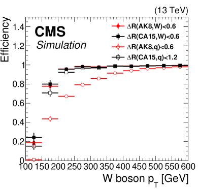
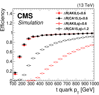
Figure 1: Matching efficiency as a function of the  of the generated particle, for hadronically decaying bosons (left) and quarks (right). This efficiency is defined as the fraction of the generated particles ( quarks or bosons) that are within $\Delta R<0.6$ with an AK8 or CA15 jet with $\pt>200\GeV$ and $\abs{\eta}<2.4$. Superimposed is the merging efficiency as a function of the generated particle when all decay products are within $\Delta R(\text{AK8},\Pq_{i})<0.6$ ($\Delta R(\text{CA15},\Pq_{i})<1.2$) with an AK8 (CA15) jet.

Finally, the is defined as the negative of the vectorial sum of the $\ptvec$ of all PF candidates in the event [52]. Its magnitude is denoted as . The jet energy scale corrections applied to the jets are propagated to .

0.5 Event selection

Several samples are used to validate the performance of the tagging algorithms in data. A single-$\mu$ signal sample is used to calibrate the quark and boson identification performance in a sample enriched in hadronically decaying quarks, as explained below. A dijet sample, dominated by light-flavor quarks and gluons, enables the study of the identification probability of background jets (misidentification rate) in a wide range of . The misidentification rate depends on the flavor of the parton that initiated the jet. Thus, in addition to the dijet sample, the single-$\gamma$ background sample is further used. The dijet and single-$\gamma$ samples differ in the light-flavor quark and gluon fractions. The former has a larger fraction of gluon jets than the latter.

Systematic effects are quantified using these samples to determine uncertainties in measurements corrected for the detector effects.

0.5.1 The single-$\mu$ signal sample

The single-$\mu$ signal sample was recorded using a single-muon trigger that selects events online based on the muon $\pt$. Candidate events are required to have exactly one muon with $\pt>55\GeV$, satisfying the identification criteria defined in Section 0.4, except for the requirement related to the isolation of leptons $I_{\text{rel}}$. In high-leptonic decays of the quarks, the lepton from the boson decay often overlaps with the jet from the quark decay, leading to large values of $I_{\text{rel}}$, causing the event to be rejected. Therefore, a custom isolation criterion is applied by requiring a minimal distance between the muon and the nearest AK4 jet, $\Delta R(\mu,\text{AK4})>0.4$, or the perpendicular component of the muon $\pt$ with respect to the nearest AK4 jet, $p_{\text{T,rel}}>25\GeV$. This has been extensively used in measurements [5] and searches [53, 54, 55, 56] involving high momentum quarks in the single-$\mu$ sample.

The AK4 jets used in this selection are clustered from PF candidates after removing muons with $\pt>55\GeV$. The custom isolation requirement results in an up to 40% increase in the statistical power of the sample. To suppress the contribution from QCD multijet processes we require $\ptmiss>50\GeV$. To enhance the sample purity in $\ttbar$ events, we require the presence of two or more AK4 jets, at least one of which is reconstructed as a jet. In addition, to probe high momentum topologies, we require the  of the leptonically decaying bosons, defined as $\ptvec(\PW)=\ptvec(\mu)+\ptvecmiss$, and the scalar  sum of the AK4 jets, denoted as $\HT$, to be greater than 250. The /candidate is the highest  AK8 or CA15 jet in the event with $\pt>200\GeV$, satisfying the criteria discussed in Section 0.4. To further improve the purity, we require the azimuthal angle $\Delta\phi$ between the AK8 or CA15 jet and the muon to be greater than 2 radians. The purity of the sample in semileptonic events is $\sim$70%; other contributions arise from QCD multijet ($\sim$15%) and +jets ($\sim$10%) processes.

0.5.2 The dijet background sample

The dijet background sample was recorded with a trigger that uses $\HT$. Events with $\HT>1000\GeV$ are selected to ensure 100% trigger efficiency. Events are required to have at least one AK8 or CA15 jet meeting the requirements presented in Section 0.4, and the absence of electrons or muons, leading to a sample dominated by jets from the QCD multijet process, which are backgrounds to the algorithms presented here.

0.5.3 The single-$\gamma$ background sample

The single-$\gamma$ background sample was collected using an isolated-single-photon trigger. Events with a photon with $\pt>200\GeV$ are selected to ensure 100% trigger efficiency. The photon is further required to satisfy the criteria presented in Section 0.4. In addition to the photon, the single-$\gamma$ sample is required to have at least one AK8 or CA15 jet and no electrons or muons. The sample consists of $\sim$80% $\Pgg\text{+jets}$ events, but only $\sim$15% QCD multijet events.

0.6 Overview of the algorithms

This section presents recently developed ML-based CMS heavy-object tagging methods. However, to understand the historical developments and their limitations, we first present tagging algorithms that do not rely on selections involving ML-based methods, but instead rely on selections based on a set of jet substructure observables (“cutoff-based” approaches). To better explore the complementarity between the jet substructure variables, alternative tagging algorithms were developed using multivariate methods. Lastly, to exploit the full potential of the CMS detector and event reconstruction, methods based on Deep Neural Networks (DNNs) are explored using either high level inputs (e.g., jet substructure observables), or lower level inputs, such as PF candidates and secondary vertices. Finally, dedicated versions of the algorithms are developed that are only loosely correlated with the jet mass. A detailed discussion of each algorithm is presented in this Section and a summary of all quark, , or boson identification algorithms is given in Table 0.6.

Summary of the CMS algorithms for the identification of hadronically decaying  quarks and , and bosons. See text for explanation of the algorithm names. The column “Subsection” indicates the subsection where the algorithm is described, and the column “jet []” indicates the jet threshold to be used in each algorithm. The ^∗ in DeepAK8 and DeepAK8-MD algorithms indicates the ability of these algorithm to also identify the decay modes of each particle.

Algorithm	Subsection	jet []	quark	boson	boson	boson
$m_{\mathrm{SD}}+{\tau_{32}}$	6.1	400	✓
$m_{\mathrm{SD}}+{\tau_{32}+\PQb}$	6.1	400	✓
$m_{\text{SD}}+{\tau_{21}}$	6.1	200	✓	✓
HOTVR	6.2	200	✓
$N_{3}\text{-}\mathrm{BDT}\,(\mathrm{CA}15)$	6.3	200	✓
$m_{\mathrm{SD}}+N_{2}$	6.3	200		✓	✓	✓
BEST	6.5	500	✓	✓	✓	✓
ImageTop	6.6	600	✓
DeepAK8(∗)	6.7	200	✓	✓	✓	✓
Jet mass decorrelated algorithms
$m_{\mathrm{SD}}+N_{2}^{\mathrm{DDT}}$	6.3	200		✓	✓	✓
double-	6.4	300			✓	✓
ImageTop-MD	6.6	600	✓
DeepAK8-MD(∗)	6.7	200	✓	✓	✓	✓

0.6.1 Substructure variable based algorithms

Historically, the high momentum quark and //boson tagging methods used by the CMS Collaboration are based on a combination of selection criteria on the jet mass and the energy distribution inside the jet [16, 17, 18, 19, 20].

The jet mass is one of the most powerful observables to discriminate quark and //boson jets from background jets (i.e., jets stemming from the hadronization of light-flavor quarks or gluons). The QCD radiation will cause a radiative shower of quarks and gluons, which will be collimated within a jet. The probability for a gluon to be radiated from a propagating quark or gluon is inversely proportional to the angle and energy of the radiated gluon. Hence, the radiated gluon will tend to appear close to the direction of the original quark or gluon. These radiated gluons tend to be soft, resulting in a characteristic “Sudakov peak” structure. This is explained in detail in Ref. [8]. Contributions from initial-state radiation, the underlying event, and pileup also contribute strongly to the jet mass, especially at larger values of $R$. As such, jet mass from QCD radiation scales as the product of the jet and $R$.

Several methods have been developed to remove soft or uncorrelated radiation from jets, a procedure generally called “grooming”. These methods strongly reduce the Sudakov peak structure in the jet mass distribution. The removal of the soft and uncorrelated radiation results in a much weaker dependence of the jet mass on its $\pt$.

The quark and //bosons have an intrinsic mass, and the jet substructure tends to be dominated by electroweak splittings [57] at larger angles than QCD. This can be exploited to separate such jets from jets arising from heavy SM particles.

The grooming method used most often in CMS is the “modified mass drop tagger” algorithm (mMDT) [58], which is a special case of the “soft drop” (SD) method [59]. This algorithm systematically removes the soft and collinear radiation from the jet in a manner that can be theoretically calculated [60, 61] (comparisons to data are found in Ref. [8]).

The first step in the SD algorithm is the reclustering of the jet constituents with the CA algorithm, and then the identification of two “subjets” within the main jet by reversing the CA clustering history. The jet is considered as the final jet if the two subjets meet the SD condition:

$$\frac{\min(p_{\text{T}1},p_{\text{T}2})}{p_{\text{T}1}+p_{\text{T}2}}>z_{\text{cut}}\left(\frac{\Delta R_{12}}{R_{0}}\right)^{\beta},$$ (1)

where $R_{0}$ is the distance parameter used in jet clustering algorithm, $p_{\text{T}1}$ ($p_{\text{T}2}$) is the of the leading (subleading) subjet and $\Delta R_{12}$ is their angular separation. The parameters $z_{\text{cut}}$ and $\beta$ define what the algorithm considers “soft” and “collinear,” respectively. The values used in CMS are $z_{\text{cut}}=0.1$ and $\beta=0$ (making this identical to the mMDT algorithm, although for notation we still denote this as SD). If the SD condition is not met, the subleading subjet is removed and the same procedure is followed until Eq. (1) is satisfied or no further declustering can be performed.

The two subjets returned by the SD algorithm are used to calculate the jet mass. Figure 2 shows the distribution of the AK8 jet mass after applying the SD algorithm ($m_{\mathrm{SD}}$) in simulated signal and background jets. The jet mass has been measured in data in previous papers by CMS for -tagged [6] and QCD jets [7, 8].

The $m_{\mathrm{SD}}$ in background jets peaks close to zero because of the suppression of the Sudakov peak [58], whereas the $m_{\mathrm{SD}}$  for signal jets peaks around the mass of the heavy SM particle (quark, or //bosons). In Fig. 2 (right), the peak around 80is from jets that contain just the two quarks from the decay and not all three quarks from the decay. Similar conclusions also hold for CA15 jets. Based on these observations, we define three regions in $m_{\mathrm{SD}}$. The “/mass region” with $65<m_{\mathrm{SD}}<105\GeV$, the “mass region” with $90<m_{\mathrm{SD}}<140\GeV$, and the “mass region” with $105<m_{\mathrm{SD}}<210\GeV$. These definitions will be used throughout this paper unless stated otherwise.

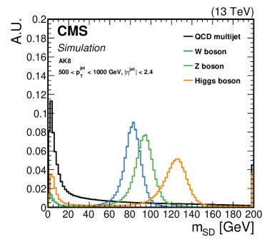
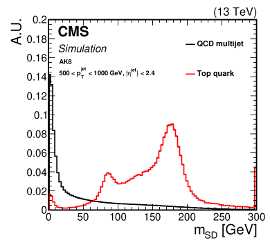
Figure 2: Comparison of the $m_{\mathrm{SD}}$ shape in signal and background AK8 jets in simulation. The fiducial selection on the jets is displayed on the plots. Signal jets are defined as jets arising from hadronic decays of //bosons (left) or quarks (right), whereas background jets are obtained from the QCD multijet sample.

An additional handle to separate signal from background events is to exploit the energy distribution inside the jet. Jets resulting from the hadronic decays of a heavy particle to $N$ separate quarks or gluons are expected to have $N$ subjets. For two-body decays like //, there are two subjets, while for quarks, there are three. In contrast, jets arising from the hadronization of light quarks or gluons are expected to only have one or two (in the case of gluon splitting) subjets. The $N$-subjettiness variables [62, 63],

$$\tau_{N}=\frac{1}{d_{0}}\displaystyle\sum_{i}p_{\mathrm{T},i}\min\left[\Delta R_{1,i},\Delta R_{2,i},\dots,\Delta R_{N,i}\right],$$ (2)

provide a measure of the number of subjets that can be found inside the jet. The index $i$ refers to the jet constituents, while the $\Delta R$ terms represent the spatial distance between a given jet constituent and the subjets. The quantity $d_{0}$ is a normalization constant. The centers of hard radiation are found by applying the exclusive algorithm [64, 65] on the jet constituents before the use of any grooming techniques. The values of the $\tau_{N}$ variables are typically small if the jet is compatible with having $N$ or more subjets. However, a more discriminating observable is the ratio of different $\tau_{N}$ variables. For this purpose, the ratio $\tau_{3}/\tau_{2}\equiv$$\tau_{32}$ is used for  quark identification, whereas the ratio $\tau_{21}$ is used for //boson identification. The distribution $\tau_{21}$ and $\tau_{32}$  for signal and background AK8 jets is shown in Fig. 3. Measured values of these distributions at CMS can also be found for light-flavor jets in Ref. [9]. Typical operating regions for $\tau_{21}$ ($\tau_{32}$) are 0.35–0.65 (0.44–0.89), which correspond to a misidentification rate after the $m_{\mathrm{SD}}$ selection of 0.1–10% for both.

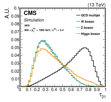
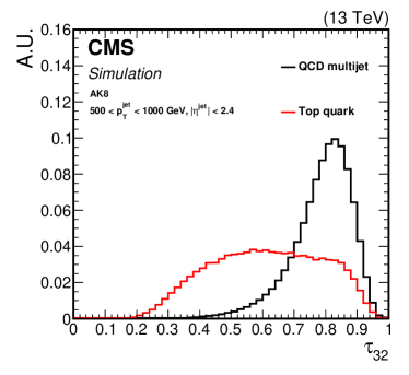
Figure 3: Comparison of the $\tau_{21}$ (left) and $\tau_{32}$ (right) shape in signal and background AK8 jets. The fiducial selection on the jets is displayed in the plots. As signal jets we consider jets stemming from hadronic decays of , , or bosons (left), or quarks (right), whereas background jets are obtained from the QCD multijet sample.

The baseline and boson (collectively referred to as boson) tagging algorithm, based on selections on $m_{\mathrm{SD}}$ and $\tau_{21}$, will be labelled as “$m_{\text{SD}}+{\tau_{21}}$” in this paper. The tagging with this method is used frequently in current analyses (e.g., in Refs. [66, 67, 68, 69]) starting at approximately 200in .

For quark tagging we studied a tagger based on $m_{\mathrm{SD}}$ and $\tau_{32}$, which will be referred to as “$m_{\mathrm{SD}}+{\tau_{32}}$”. An additional improvement in the performance of the quark identification is achieved by applying the CSVv2 tagging algorithm discussed in Section 0.4 on the subjets returned by the SD algorithm. In the studies presented in this paper we require at least one of the two subjets to pass the loose working point of the CSVv2 algorithm, corresponding to the quark jet identification efficiency $\sim$85%, with a misidentification rate for light-flavor quarks and gluon jets of $\sim$10%, and $\sim$60% for the quark jets. This version of the baseline quark tagging algorithm is referred to as “$m_{\mathrm{SD}}+{\tau_{32}+\PQb}$”. Top-quark tagging with this method is used extensively in physics analyses (e.g., in Refs. [56, 70, 71, 72]) tagging high-quarks, which start to merge into the AK8 cone at $\pt\sim 350\GeV$ and are 50% efficient at around 600. For applications below this mass range, analyses can profit from the larger (or variable) $R$ clustering algorithms discussed in the following sections.

0.6.2 Heavy object tagger with variable $R$

The heavy object tagger with variable $R$ (HOTVR) [73] is a new cutoff-based algorithm for the identification of jets originating from hadronic decays of boosted heavy objects. It introduces a new jet clustering technique with a variable $R$ and removal of soft contributions during the clustering. The clustering is similar to other standard sequential clustering algorithms such as the CA algorithm, where particles are sequentially added. However, instead of a fixed $R$, HOTVR uses a -dependent $R$ ($R_{\text{HOTVR}}$), defined as:

$$R_{\text{HOTVR}}=\begin{cases}R_{\text{min}},\text{ for }\rho/\pt<R_{\text{min}}\\ R_{\text{max}},\text{ for }\rho/\pt>R_{\text{max}}\\ \rho/\pt,\text{ elsewhere}\\ \end{cases}.$$ (3)

The value of $\rho$ is chosen to correspond to a typical energy scale of the event ($\mathcal{O}(100)\GeV$). In the case of $\rho\to 0$, the algorithm is identical to the CA algorithm for $R=R_{\mathrm{min}}$, whereas for $\rho\to\infty$ it is identical to the CA algorithm for $R=R_{\text{max}}$. Higher values of $\rho$ result in larger jet sizes. The parameters $R_{\text{min}}$ and $R_{\text{max}}$ are introduced for robustness of the algorithm with respect to detector effects.

Inspired by Ref. [73], at each clustering step, the invariant mass $m_{ij}$ between two subjets $i$ and $j$ is calculated. If $m_{ij}$ is greater than a threshold, $\mu$, the following condition is verified:

$$\theta m_{ij}>\max(m_{i},m_{j}),$$ (4)

where $m_{i}$ and $m_{j}$ are the masses of the two subjets, and $\theta$ is a parameter that determines the strength of the condition and ranges from 0 to 1. If the condition in Eq. (4) is not fulfilled, the subjet with the lower mass is discarded; otherwise depending on the relative  difference of the subjets they are either combined into a single subjet or the softer one is discarded. The algorithm continues until no other subjet is found. The detailed description of the HOTVR algorithm is presented in Ref. [73]. Table 0.6.2 lists the values of HOTVR parameters used in CMS. In the CMS implementation, HOTVR jets are clustered using PUPPI corrected PF candidates.

Summary of the HOTVR parameters used in CMS. The $\pt{}_{\text{sub}}$ is the minimum threshold of each subjet. $R_{\text{min}}$ $R_{\text{max}}$ $\rho$ [] $\mu$ [] $\pt{}_{\text{sub}}$ [] $\theta$ 0.1 1.5 600 30 30 0.7

The HOTVR clustering algorithm is currently being explored in CMS for quark identification. The jets returned by HOTVR (i.e., “HOTVR jets”) are required to have mass consistent with $m_{\PQt}$, namely $140<m_{\text{HOTVR}}<220\GeV$, and at least three subjets, $N_{\text{sub,~{}HOTVR}}\geq 3$, the minimum pairwise mass of which should be $m_{\text{disub,~{}min}}>50\GeV$. In addition, the of the hardest subjet must be less than 80% of the HOTVR jet . Lastly, to further improve the discrimination, $\tau_{32}<0.56$ is required. The shape comparison of the main variables of the HOTVR algorithm for signal and background, for different parton ranges, is shown in Fig. 4.

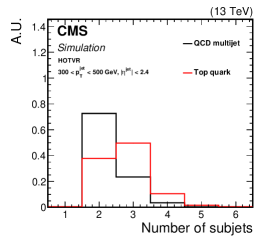
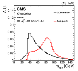
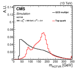
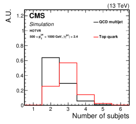
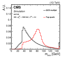
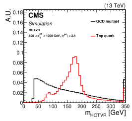
Figure 4: Shape comparison of the main variables of the HOTVR algorithm for signal and background jets, in two different regions of the jet as displayed in the plots.

0.6.3 Energy correlation functions

A new set of $N$-prong identification algorithms, the generalized energy correlation functions (ECFs) [74], are now used by the CMS Collaboration. The ECFs explore the energy distribution inside a jet by aiming to quantify the number of centers of hard radiation using an axis-free approach, differing from the axis-dependent definition used by $N$-subjettiness, which reduces the dependence of the observable on the jet . This allows the exploration of complementary information between the two techniques.

For a jet containing $N_{\text{C}}$ particles, an ECF is defined as:

$${}_{q}e_{N}^{\beta}=\sum_{1\leq i_{1}<i_{2}<\cdots<i_{N}\leq N_{\text{C}}}\left[\prod_{1\leq k\leq N}\frac{\pt^{i_{k}}}{\pt^{J}}\right]\prod_{m=1}^{q}\min_{i_{j}<i_{k}\in\{i_{1},i_{2},\cdots,i_{N}\}}^{(m)}\left\{\Delta R_{i_{j},i_{k}}^{\beta}\right\},$$ (5)

where $1\leq i_{1}<i_{2}<\cdots<i_{N}\leq N_{\text{C}}$ range over the jet constituents. The symbols $\pt^{i_{k}}$ and $\pt^{J}$ are the of the constituent $i_{k}$ and the of the jet, respectively. The notation $\text{min}^{(m)}$ refers to the $m$th smallest element, and $\Delta R_{i_{j},i_{k}}$ is the angular distance between constituents $i_{j}$ and $i_{k}$. The parameters $N$ and $q$ must be positive integers, and the exponent $\beta$ must be positive as well. For a concrete example, we calculate the ECF corresponding to $q=2,N=3,\beta=1$. This ECF tests the compatibility of a jet with three centers of hard radiation, but only considering the two smallest angles ($q=2$):

$${}_{2}e_{3}^{1}=\sum_{1\leq a<b<c\leq M}\frac{\pt^{a}\pt^{b}\pt^{c}}{(\pt^{J})^{3}}\min\{\Delta R_{ab}\Delta R_{ac},\Delta R_{ab}\Delta R_{bc},\Delta R_{bc}\Delta R_{ac}\}.$$ (6)

Moreover, there is the possibility to select subsets of the jet that contain large energy fractions and pairwise opening angles only if the size of the subset is less than or equal to the number of the centers of radiation in the jet. In general, a jet with $N$ centers of radiation has $e_{N}\gg e_{M}$, for $M>N$.

The ECFs for 3-prong decay identification

The ratios of type $(N=4)/(N=3)$ can identify the hadronic 3-body decays, such as those of quarks. Reference [74] proposes to use the specific ratio $N_{3}$ for this purpose:

$$N_{3}^{(\beta)}=\frac{{}_{2}e_{4}^{\beta}}{(_{1}e_{3}^{\beta})^{2}}.$$ (7)

Since a jet contains $N_{C}\sim\mathcal{O}(\pt/\mathrm{GeV})$ constituents, and the sum has $\binom{N_{C}}{N}$ terms, it is prohibitively expensive to compute $e(N=4)$ on high- jets. For example, about 10–15% of CA15 jets with $\pt\sim 500\GeV$ have more than 100 particles. However, we find that these functions are dominated by the hardest particles, and therefore limiting to the 100 hardest particles makes the calculation tractable without significant performance degradation.

In our reconstruction, the ECF ratios are calculated for jets after the SD grooming is applied, which improves the stability of ECF as a function of jet mass and . An example of the ECF ratios is shown in the left plot of Fig. 5 for simulated quark and QCD jets. The ECF ratios are measured in data in Ref. [9] showing reasonable agreement with the expectation from simulation. While $N_{3}$ is designed to have comparable performance with $\tau_{32}$, its dependence on is reduced.

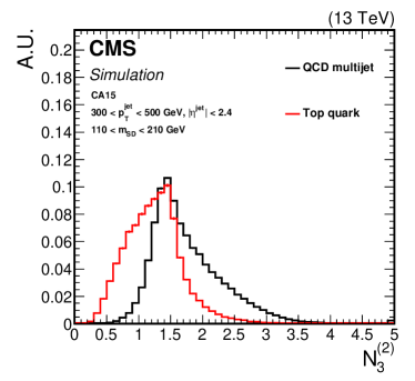
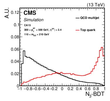
Figure 5: Comparison of the distribution of $N_{3}^{(2)}$ (left) and the $N_{3}\text{-}\mathrm{BDT}\,(\mathrm{CA}15)$ discriminant (right) in quarks jets (signal) and jets from QCD multijet processes (background).

Therefore, a set of ECFs is chosen based on the improvement in the performance of the tagging algorithm, while in parallel maintaining small dependence on jet . Despite the fact that the terms of the ECFs are dimensionless, the angular component of ECF function is modified according to the boost of the parent particle. Hence, scale invariant ECF ratios are constructed by only considering those ratios that satisfy:

$$\frac{{}_{a}e_{N}^{\alpha}}{(_{b}e_{M}^{\beta})^{x}}\text{, where }M\leq N\text{ and }x=\frac{a\alpha}{b\beta}.$$ (8)

Only ratios that are not highly correlated among themselves are considered for the quark tagging algorithm, and ECF ratios that are not well described by simulation are discarded. The following 11 ECF ratios are finally selected:

$$\frac{{}_{1}e_{2}^{(2)}}{\Bigl{(}{}_{1}e_{2}^{(1)}\Bigr{)}^{2}},\frac{{}_{1}e_{3}^{(4)}}{{}_{2}e_{3}^{(2)}},\frac{{}_{3}e_{3}^{(1)}}{\Bigl{(}{}_{1}e_{3}^{(4)}\Bigr{)}^{3/4}}, \frac{{}_{3}e_{3}^{(1)}}{\Bigl{(}{}_{2}e_{3}^{(2)}\Bigr{)}^{3/4}},\frac{{}_{3}e_{3}^{(2)}}{\Bigl{(}{}_{3}e_{3}^{(4)}\Bigr{)}^{1/2}},$$ (9)

$$\frac{{}_{1}e_{4}^{(4)}}{\Bigl{(}{}_{1}e_{3}^{(2)}\Bigr{)}^{2}},\frac{{}_{1}e_{4}^{(2)}}{\Bigl{(}{}_{1}e_{3}^{(1)}\Bigr{)}^{2}},\frac{{}_{2}e_{4}^{(1/2)}}{\Bigl{(}{}_{1}e_{3}^{(1/2)}\Bigr{)}^{2}}, \frac{{}_{2}e_{4}^{(1)}}{\Bigl{(}{}_{1}e_{3}^{(1)}\Bigr{)}^{2}},\frac{{}_{2}e_{4}^{(1)}}{\Bigl{(}{}_{2}e_{3}^{(1/2)}\Bigr{)}^{2}},\frac{{}_{2}e_{4}^{(2)}}{\Bigl{(}{}_{1}e_{3}^{(2)}\Bigr{)}^{2}}.$$

In addition to the ECFs, two jet substructure observables are employed to further distinguish quark jets from light quarks or gluons. The first observable is $\tau_{32}$ calculated for CA15 jets, after applying the SD grooming, defined as $\tau_{32}^{\mathrm{SD}}$   and the second is the $f_{\text{rec}}$ variable of the HEPTopTagger algorithm [75, 76, 77], which quantifies the difference between the reconstructed boson and quark masses and their expected values, and is defined as:

$$f_{\text{rec}}=\min_{i,j}\left|\frac{m_{ij}/m_{123}}{m_{\text{W}}/m_{\text{t}}}-1\right|,$$ (10)

where $i,j$ range over the three chosen subjets, $m_{ij}$ is the mass of subjets $i$ and $j$, and $m_{123}$ is the mass of all three subjets.

The ECF-based quark tagger, referred to as “$N_{3}\text{-}\mathrm{BDT}\,(\mathrm{CA}15)$”, is based on a boosted decision tree (BDT) [78] with the 11 ECF ratios, the $\tau_{32}^{\mathrm{SD}}$, and the $f_{\text{rec}}$ as inputs. The $N_{3}\text{-}\mathrm{BDT}\,(\mathrm{CA}15)$ algorithm was trained using jets with $110<m_{\mathrm{SD}}<210\GeV$. To avoid possible bias in the identification performance due to differences in the spectrum of the signal (quarks) and background (light quarks or gluons) jets, their contributions are reweighted such that they have a flat distribution in jet .

Figure 5 (right) shows a comparison of the $N_{3}\text{-}\mathrm{BDT}\,(\mathrm{CA}15)$ discriminant distribution between signal and background jets. The final $N_{3}\text{-}\mathrm{BDT}\,(\mathrm{CA}15)$ algorithm also requires at least one of the two subjets returned by the SD method to be identified as a jet by the CSVv2 algorithm using the loose working point. The ECF BDT tagger is used for quark jet identification in the context of dark matter production in association with a single quark in the $\pt>250\GeV$ range [79].

The ECFs for 2-prong decay identification

The use of ECFs is also explored for the identification of 2-prong decays, such as hadronic decays of //bosons. In this case, the signal jets have a stronger 2-point correlation than a 3-point correlation and the discriminant variable $N_{2}^{1}$ can be used to separate jets originating from //bosons. The $N_{2}$ variable is constructed via the ratio

$$N^{1}_{2}\equiv N_{2}^{1}=\frac{{}_{2}e_{3}^{1}}{(_{1}e_{2}^{1})^{2}},$$ (11)

and shows similar performance to $N$-subjettiness ratio $\tau_{21}$, with the advantage that it is more stable as a function of the jet mass and . This method is referred to as “$m_{\mathrm{SD}}+N_{2}$”.

A decorrelation procedure is further applied to avoid distorting the jet mass distribution when a selection based on $N_{2}$ is made. We design a transformation from $N_{2}$ to $N_{2}^{\text{DDT}}$, where DDT stands for “designed decorrelated tagger” described in Ref. [15]. The transformation is defined as a function of the dimensionless scaling variable $\rho=\ln(m_{\mathrm{SD}}^{2}/\pt^{2})$ and the jet :

$$N_{2}^{\text{DDT}}(\rho,\pt)=N_{2}(\rho,\pt)-N_{2}^{(X\%)}(\rho,\pt),$$ (12)

where $N_{2}^{(X\%)}$ is the $X$ percentile of the $N_{2}$ distribution in simulated QCD events. This ensures that the selection $N_{2}^{\text{DDT}}<0$ yields a constant QCD background efficiency of $X\%$ across the mass and range considered with no loss in performance. The value $X=5$ is used throughout this paper, following the choice in [80]. The distributions of $N_{2}$ and $N_{2}^{\text{DDT}}$ in signal and background jets are shown in Fig. 6. Signal jets have smaller values and background jets have larger values. The $N_{2}^{\text{DDT}}$ is used for tagging with in excess of 500in the search for light dijet resonances [80].

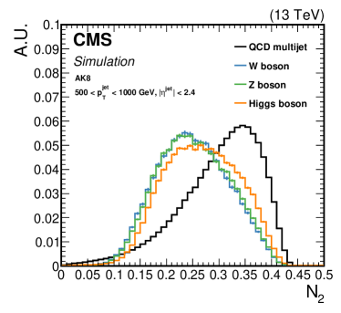
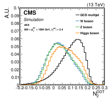
Figure 6: Distributions of the $m_{\mathrm{SD}}+N_{2}$ (left) and $m_{\mathrm{SD}}+N_{2}^{\mathrm{DDT}}$ (right) in signal and background jets.

The $m_{\mathrm{SD}}+N_{2}^{\mathrm{DDT}}$ observable was used and validated in several analyses, including the ones described in Refs.[80, 81].

0.6.4 The double-$\PQb$ tagger

The standard tagging tools, such as the CSVv2 discussed in Section 0.4, can be applied to the subjets returned by the SD algorithm applied to AK8 jets. Characteristic examples are the $m_{\mathrm{SD}}+{\tau_{32}+\PQb}$ and $N_{3}\text{-}\mathrm{BDT}\,(\mathrm{CA}15)$ algorithms. However, these tools have limitations in certain topologies, for example when the two subjets become very collimated. The “double-” tagger was developed to specifically target Higgs decays to pairs of quarks in the boosted regime [20]. While it utilizes many of the variables used in the standard CSVv2 tagging algorithm, it also employs variables related to the track properties, such as the track impact parameter and its significance, the positions of secondary vertices, and information from the two-secondary-vertex system, among others listed in Ref. [20]. An important feature of the double-algorithm is that it uses the $N$-subjettiness axes, defined in Eq. (2), for $N=2$, to group the tracks to the direction of the partons giving rise to the two subjets. The double-variables are then used as inputs to a BDT. A key feature of the double-algorithm is that it is designed to minimize the dependence of the BDT discriminant on the jet mass and , thus making it suitable for other topologies such as decays of boosted bosons to bottom quarks [81].

The performance of the double-tagger in simulation is detailed in Ref. [20] using boson jets as signal, and single-, double-jets from gluon splitting to a pair of quarks, and light-flavor quark or gluon jets. The $\PH\to\bbbar$ identification efficiency is $\sim$25% ($\sim$70%) for $\sim$1% ($\sim$10%) misidentification rate [20].

The double-tagger performance in data is studied in [20] using data in a recent inclusive search for the Higgs boson in the $\bbbar$ decay mode [81]. In that analysis, the boson was observed for the first time in the single-jet topology and $\bbbar$ decay mode, with a rate consistent within uncertainties with the SM expectation, validating the double-tagging algorithm for the Higgs boson measurements and future searches.

The double-tagger will serve as a reference for the performance of the new methods explored in CMS.

0.6.5 Boosted event shape tagger

The boosted event shape tagger (BEST) [82] is a multi-classification algorithm designed to discriminate hadronic decays of high-quarks and //bosons from jets arising from quarks, light flavor quarks, and gluons. The original algorithm was demonstrated using generator-level particles and efficiently separated jets originating from //bosons, quarks, and jets. The algorithm has been extended and deployed for use in the CMS experiment, adding an additional category to discriminate jets from light-flavor quarks and gluons.

The BEST algorithm obtains discrimination on a jet-by-jet basis by transforming the entire set of jet constituents four times, each with a different boost vector. The boost vectors are obtained by assuming the jet originating from one of the heavy objects under consideration (///). The jet momentum is held constant while the mass of the jet is adjusted to the theoretical value of the corresponding particle. This results in four distributions of constituents that can be used to discriminate between particle origins. If a jet did originate from one of the hypothesized heavy objects, its jet constituents will, in general, be more isotropic in the rest frame of that particle. By examining the differences between heavy object hypotheses, discrimination is obtained between the categories of interest (/////other).

In total, 59 quantities are used to train a neural network (NN) and classify the AK8 jets. The variables are listed in Table 1. For each boost transformation, we calculate the following observables: Fox–Wolfram moments [83]; aplanarity, sphericity, and isotropy quantities based on the eigenvalues of sphericity tensor, as defined in Ref. [84]; and jet thrust [85]. Additionally, in each boost hypothesis, AK4 subjets are clustered from the constituents and used to compute pairwise subjet masses for the leading three subjets, as well as the combined mass of the leading four subjets $m_{1234}$. These AK4 subjets are also used to compute the longitudinal asymmetry $A_{L}$, defined as the ratio of the sum of longitudinal components of the AK4 subjet momenta to the sum of the total AK4 subjet momenta. In addition to these quantities evaluated for each set of jet constituents, the $m_{\mathrm{SD}}$, rapidity, charge, $\tau_{32}$, $\tau_{21}$, and the CSVv2 discriminant for each subjet provide additional inputs for each set of boosted jet constituents.

The NN is trained with the scikit-learn package [86] using the MLPClassifier module. The network architecture is fully connected and consists of 3 hidden layers with 40 nodes in each layer using a rectified linear unit (ReLU) [87] activation function. The six output nodes correspond to the 6 particle species of interest. We use 500 000 jets to train the network, split evenly between the 6 training samples. The training is performed using the Adam [88] optimizer to minimize the cross entropy loss with a constant learning rate of 0.001. Cross entropy is a measure of the difference (entropy) between two probability distributions and it is used for optimizing a classification model. The BEST /////other multi classification is currently used for tagging high-jets in the search for vector-like quark pair production [69].

Table 1: List of input quantities used for the training and evaluation of the BEST algorithm on AK8 jets.

BEST training quantities
Jet charge	Fox–Wolfram moment $H_{1}/H_{0}$ (,,,)	$m_{12}$ (,,,)
Jet $\eta$	Fox–Wolfram moment $H_{2}/H_{0}$ (,,,)	$m_{23}$ (,,,)
Jet $\tau_{21}$	Fox–Wolfram moment $H_{3}/H_{0}$ (,,,)	$m_{13}$ (,,,)
Jet $\tau_{32}$	Fox–Wolfram moment $H_{4}/H_{0}$ (,,,)	$m_{1234}$ (,,,)
Jet soft-drop mass	Sphericity (,,,)	$A_{L}$ (,,,)
Subjet 1 CSV value	Aplanarity (,,,)
Subjet 2 CSV value	Isotropy (,,,)
Maximum subjet CSV value	Thrust (,,,)

0.6.6 Identification using particle-flow candidates: ImageTop

Recent studies, e.g., in Ref. [89], have shown that jet identification algorithms deploying ML methods directly on the jet constituents yield significantly improved performance compared to traditional algorithms.

To this end, the “ImageTop” quark identification algorithm was developed. The ImageTop algorithm closely follows the network framework described in Ref. [89], which is an optimization based on the DeepTop framework described in Ref. [90]. This tagging approach uses standard image recognition techniques based on two-dimensional convolutional neural networks (CNNs) to discriminate quark jets from QCD jets. This is performed by pixelizing the jet energy deposits and define different channels based on relevant detector information. Before pixelization, the centroid of the jet is shifted to the origin and then a rotation is performed to make the major principal axis vertical. The image is then flipped along both the horizontal and vertical axes as appropriate such that the maximum intensity is in the lower-left quadrant. After this, the image intensity is normalized and the image is pixelized using $37{\times}37$ pixels with a total $\Delta\eta=\Delta\phi=3.2$, with channels split into neutral , track , number of muons, and of tracks as an analogue to colors used in image recognition. The network architecture uses a layer of 128 feature maps with a $4{\times}4$ kernel followed by a second convolutional layer of 64 feature maps each. Then a max-pooling layer with a $2{\times}2$ reduction factor is used, followed by two more consecutive convolutional layers with 64 features maps followed by another max-pooling layer. A zero-padding in each convolutional layer is used to correct for image-border effects. In the last pooling layer, the 64 maps are flattened into a single one that is passed into a set of three fully connected dense layers, one of 64 neurons, and two more with 256 neurons. The training is performed using the Tensorflow [91] software package using the AdaDelta optimizer [92] with a learning rate of 0.3, a minibatch size of 128, and the binary cross entropy loss function.

The tagger is modified to use the PF candidates contained in the AK8 jets as inputs, with the colors being the of the PF candidates for the full greyscale image, and a separate color for each PF candidate flavor, namely charged and neutral hadrons, photons, electrons, and muons. The pixelized greyscale images used in the ImageTop network for QCD and quark jets are shown in Fig. 7. The characteristic flavor of the quark decay is included by applying the DeepFlavor [93] tagging algorithm to the SD subjets of the AK8 jet. The subjet tagging outputs include the probability of the jet to originate from the following six sources: quark, $\bbbar$ pair, leptonic decays, quark, light-flavor quark, or gluon. These output probabilities calculated for both subjets along with $m_{\mathrm{SD}}$, are used as inputs (13 in total) into a 64-neuron dense layer and merged with the previous flattened CNN layer and finally input into three fully connected layers of 256 neurons each. The factorization of the flavor discrimination is important for the versatility of the network, allowing for the flavor identification to be easily removed or validated in parallel, which can be necessary for the validation of objects with no SM analog. The diagram of the CMS application of this NN can be seen in Fig. 8.

The training is performed for jets in the $\pt>600\GeV$ region. To sustain the ImageTop performance over a wide range of $\pt(\text{jet})$, the image is adaptively zoomed based on $\pt(\text{jet})$ to account for the increased collimation of the quark decay products at high Lorentz boosts and maintain a static pixel size. The functional form of the zoom is extracted from the average $\Delta R$ of the three generator-level hadronic quark decay products, and the jet energy deposits are corrected to make this constant on average, as evaluated from a fit using the inverse jet functional form $f(\pt)=0.066+264/\pt$.

A jet bias is further reduced by ensuring that the input distributions for signal and background jets are similarly shaped by probabilistically removing QCD events based on the ratio of quark and QCD jet distributions when training the nominal ImageTop tagger. The mass correlation of the tagger is reduced by additionally constraining $m_{\mathrm{SD}}$ in a similar manner to define a new discriminator, which will be referred to as “ImageTop-MD”. Since the inputs are relatively simple and do not exhibit secondary mass correlation, this passive approach for decorrelating the ImageTop network is sufficient to remove the mass bias in the fiducial training region ($\pt>600\GeV$ and $\abs{\eta}<2.4$). This method of mass decorrelation also leads to a factorized sensitivity where the sensitivity of the full ImageTop network in the quark mass region is closely approximated by the sensitivity of the mass-decorrelated version after including a mass selection.

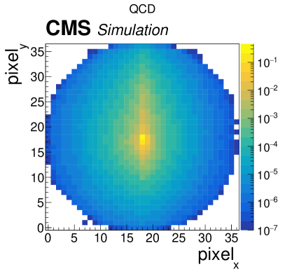
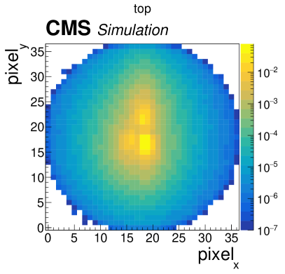
Figure 7: The pixelized images used in the ImageTop network with PF candidate colors summed together (“greyscale”) for QCD (left) and quark (right) jets. The $x$ and $y$ axes are the pixel number, and roughly scale with $\Delta R$. The $\PZ$ axis is the intensity of the greyscale image in the given pixel, related to the PF candidate $\pt$, and has been normalized to unity. This figure shows an ensemble of overlaid images after the image post processing; we can see clear differences between the QCD jet energy and quark deposition patterns.

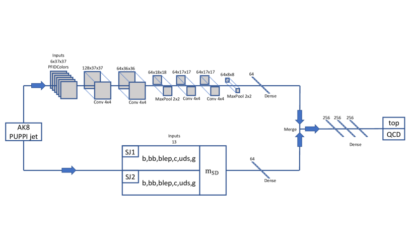
Figure 8: The ImageTop network architecture. The neural network inputs are the 37x37 pixelized PF candidate map, which is split into colors based on the PF candidate flavor, and the DeepFlavor subjet tags applied to both subjets. The pixelized images are sent through a two-dimensional CNN, and the subjet tags are inputs to a dense layer. After flattening the CNN, the two networks are taken as input to three dense layers and finally to the two-node output, which is used as the top tagging discriminator.

0.6.7 Identification using particle-flow candidates: DeepAK8

An alternative approach to exploit particle-level information directly with customized ML methods is the “DeepAK8” algorithm, a multiclass classifier for the identification of hadronically decaying particles with five main categories, ////other. To increase the versatility of the algorithm, the main classes are further subdivided into the minor categories corresponding to the decay modes of each particle (e.g., $\PZ\to\bbbar$, $\PZ\to\ccbar$ and $\PZ\to\qqbar$).

In the DeepAK8 algorithm, two lists of inputs are defined for each jet. The first list (the “particle” list) consists of up to 100 jet constituent particles, sorted by decreasing . Typically less than 5% of the jets have more than 100 reconstructed particles, therefore restricting to the 100 hardest particles results in a negligible loss of performance. Measured properties of each particle, such as the , the energy deposit, the charge, the angular separation between the particle and the jet axis or the subjet axes, etc., are included to help the algorithm extract features related to the substructure of the jet. For charged particles, additional information measured by the tracking detector is also included, such as the displacement and quality of the tracks, etc. These inputs are particularly useful to enable the algorithm to extract features related to the presence of heavy-flavor (or ) quarks. In total, 42 variables are included for each particle in the “particle” list. A secondary vertex (SV) list consists of up to 7 SVs, each with 15 features, such as the SV kinematics, the displacement, and quality criteria. The SV list helps the network to extract features related to the heavy-flavor content of the jet. The elements of the SV list as sorted based on the two-dimensional impact parameter significance (S${}_{\text{IP2D}}$).

A significant challenge posed by the direct use of particle-level information is a substantial increase in the number of inputs. Additionally, the correlations between these inputs are of vital importance. Therefore, an algorithm that can both process the inputs efficiently and exploit the correlations effectively is required. A customized DNN architecture is thus developed in DeepAK8 to fulfill this requirement. As illustrated in Fig. 9, the architecture consists of two steps. In the first step, two one-dimensional CNNs are applied to the particle list and the SV list in parallel to transform the inputs and extract useful features. In the second step, the outputs of these CNNs are combined and processed by a simple fully connected network to perform the jet classification. The CNN structure in the first step is based on the ResNet model [94], but adapted from two-dimensional images to one-dimensional particle lists. The CNN for the particle list has 14 layers, and the one for the SV list has 10 layers. A convolution window of length 3 is used, and the number of output channels in each convolutional layer ranges between 32 to 128. The ResNet architecture allows for an efficient training of deep CNNs, thus leading to a better exploitation of the correlations between the large inputs and improving the performance. The CNNs in the first step already contain strong discriminatory ability, so the fully connected network in the second step consists of only one layer with 512 units, followed by a ReLU activation function and a Dropout [95] layer of 20% drop rate. The NN is implemented using the MXNet package [96] and trained with the Adam optimizer to minimize the cross-entropy loss. A minibatch size of 1024 is used, and the initial learning rate is set to 0.001 and then reduced by a factor of 10 at the 10th and 20th epochs to improve convergence. The training completes after 35 epochs. A sample of 50 million jets is used, of which 80% are used for training and 20% for validation. Jets from different signal and background samples are reweighted to yield flat distributions in to avoid any potential bias in the training process. The DeepAK8 algorithm is designed for jets with $\pt>200\GeV$ and typical operating regions for which the misidentification rate is greater than 0.1%.

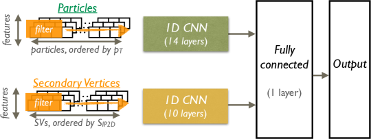
Figure 9: The network architecture of DeepAK8.

A mass-decorrelated version of DeepAK8

As will be discussed in Section 0.7, background jets selected by the DeepAK8 algorithm exhibit a modified mass distribution similar to that of the signal. The mass of a jet is one of the most discriminating variables and, although it is not directly used as an input to the algorithm, the CNNs are able to extract features that are correlated to the mass to improve the discrimination power. However, such modification of the mass distribution may be undesirable (as described in Ref. [15]) if the mass variable itself is used for separating signal and background processes. Thus, an alternative DeepAK8 algorithm, “DeepAK8-MD”, is developed to be largely decorrelated with the mass of a jet, while preserving the discrimination power as much as possible using an adversarial training approach [97]. Jets from different signal and background samples are also weighted to yield flat distributions in both and $m_{\mathrm{SD}}$ to aid the training.

The architecture of DeepAK8-MD is shown in Fig. 10. Compared to the nominal version of DeepAK8, a mass prediction network is added with the goal of predicting the mass of a background jet from the features extracted by the CNNs. The mass prediction network consists of 3 fully-connected layers, each with 256 units and a SELU activation function [98]. It is trained to predict the $m_{\mathrm{SD}}$ of background jets to the closest 10value between 30 and 250by minimizing the cross-entropy loss. When properly trained, the mass prediction network becomes a good indicator of how strongly the features extracted by the CNNs are correlated with the mass of a jet, because the stronger the correlation is, the more accurate the mass prediction will be. With the introduction of the mass prediction network, the training target of the algorithm can be modified to include the accuracy of the mass prediction for the background jets as a penalty, therefore preventing the CNNs from extracting features that are correlated with the mass. In this way, the final prediction of the algorithm also becomes largely independent of the mass. As the features extracted by the CNNs evolve during the training process, the mass prediction network itself needs to be updated regularly to adapt to the changes of its inputs and remain as an effective indicator of mass correlation. Therefore, for each training step of the DeepAK8 network (the Particle and SV CNNs and the 1-layer fully-connected network), the mass prediction network is trained for 10 steps. Each training step corresponds to a minibatch of 6000 jets. A large minibatch size is used to reduce statistical fluctuation on the mass correlation penalty evaluated by the mass prediction network, since only background jets are used in the evaluation. Both the DeepAK8 network and the mass prediction network are trained with the Adam optimizer. A constant learning rate of 0.001 (0.0001) is used for the training of the DeepAK8 (mass prediction) network.

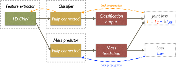
Figure 10: The network architecture of DeepAK8-MD.

Forcing the algorithm to be decorrelated with the jet mass, inevitably leads to a loss of discrimination power, and the resulting algorithm is a balance between performance and mass independence. Because the training of DeepAK8-MD is carried out only on jets with $30<m_{\mathrm{SD}}<250\GeV$, jets with $m_{\mathrm{SD}}$ outside this range should be removed when using DeepAK8-MD.

0.7 Performance in simulation

As presented in Section 0.6, a variety of algorithms have been developed by the CMS Collaboration to identify the hadronic decays of /// bosons and quarks. To gain an initial understanding of the tagging performance and the complementarity between the different approaches, the algorithms were studied in simulated events. The performance of the algorithms is evaluated using the signal and background efficiencies, $\epsilon_{\text{S}}$ and $\epsilon_{\text{B}}$, respectively, as a figure of merit. The efficiencies $\epsilon_{\mathrm{S}}$ and $\epsilon_{\mathrm{B}}$ are defined as:

$$\epsilon_{\mathrm{S}}=\frac{N^{\text{tagged}}_{\text{S}}}{N^{\text{total}}_{\text{S}}}~{}~{}~{}\text{and}~{}~{}~{}\epsilon_{\mathrm{B}}=\frac{N^{\text{tagged}}_{\text{B}}}{N^{\text{total}}_{\text{B}}},$$ (13)

where $N^{\text{tagged}}_{S}$ ($N^{\text{tagged}}_{B}$) is the number of signal (background) jets satisfying the identification criteria of each algorithm, and $N^{\text{total}}_{S}$ ($N^{\text{total}}_{B}$) is the total number of generated particles considered to be signal (background). Hadronically decaying //bosons or quarks are signal, whereas quarks (excluding  quarks) and gluons from the QCD multijet process are background.

First, for each algorithm, the $\epsilon_{\mathrm{B}}$ as a function of $\epsilon_{\mathrm{S}}$ is evaluated in terms of a receiver operating characteristic (ROC) curve. Figures 11–14 summarize the ROC curves of all algorithms for the identification of  quarks, and , , and bosons, respectively. The comparisons are performed at low and high values of the generated particle . The fiducial selection criteria applied to the generator-level particles are displayed in the plots. For the cutoff-based algorithms, namely $m_{\mathrm{SD}}+{\tau_{32}}$, $m_{\mathrm{SD}}+{\tau_{32}+\PQb}$, $m_{\text{SD}}+{\tau_{21}}$, $m_{\mathrm{SD}}+N_{2}$, and $m_{\mathrm{SD}}+N_{2}^{\mathrm{DDT}}$, all selections except the selection on $\tau_{32}$, $\tau_{21}$, or $N_{2}$, are applied, as described in Sections 0.6.1 and 0.6.3.

In tagging, the addition of the subjet $\PQb$ tagging in the $m_{\mathrm{SD}}+{\tau_{32}}$ algorithm reduces the misidentification probability for  quarks by up to $\sim$50% depending on the . The performance of the HOTVR algorithm lies between $m_{\mathrm{SD}}+{\tau_{32}}$ and $m_{\mathrm{SD}}+{\tau_{32}+\PQb}$, and the $N_{3}\text{-}\mathrm{BDT}\,(\mathrm{CA}15)$ algorithm shows improved performance compared to these algorithms, particularly in the low-range. The improved performance stems from the usage of the ECFs, which provide complementary information to $\tau_{32}$. Particularly in the low-region, the gain is mainly due to the use of larger-cone jets (i.e., jets clustered with $R=1.5$). The BEST algorithm targets the high-regime and shows similar performance to the ECF algorithm in this regime. The best discrimination is achieved with algorithms based on lower-level information, namely the ImageTop and DeepAK8 algorithms. ImageTop and DeepAK8-MD yield comparable performance in the low and high regions. The best performance in terms of ROC curves is achieved with the nominal version of DeepAK8 over the entire region.

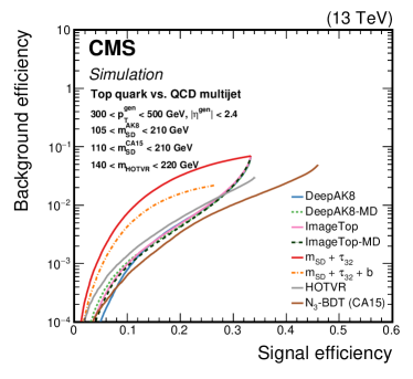
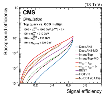
Figure 11: Comparison of the identification algorithms for hadronically decaying  quark in terms of ROC curves in two regions based on the  of the generated particle; Left: $300<\pt<500\GeV$, and Right: $1000<\pt<1500\GeV$. Additional fiducial selection criteria applied to the jets are listed on the plots.

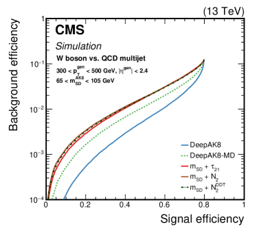
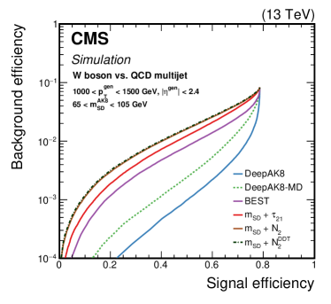
Figure 12: Comparison of the identification algorithms for hadronically decaying  boson in terms of ROC curves in two regions based on the  of the generated particle; Left: $300<\pt<500\GeV$, and Right: $1000<\pt<1500\GeV$. Additional fiducial selection criteria applied to the jets are listed on the plots.

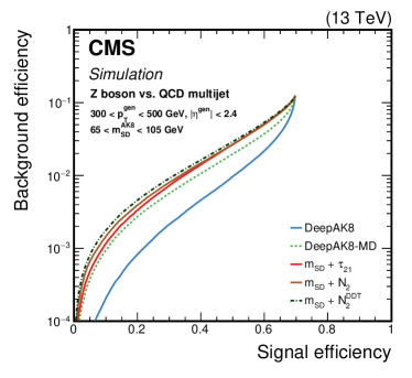
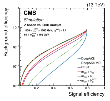
Figure 13: Comparison of the identification algorithms for hadronically decaying  boson in terms of ROC curves in two regions based on the  of the generated particle; Left: $300<\pt<500\GeV$, and Right: $1000<\pt<1500\GeV$. Additional fiducial selection criteria applied to the jets are listed on the plots.

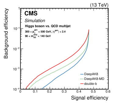
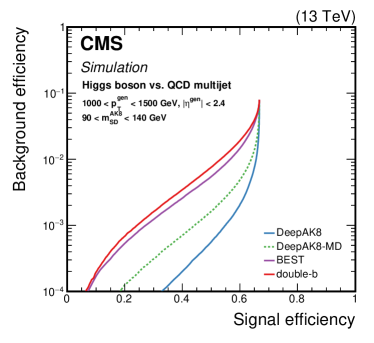
Figure 14: Comparison of the identification algorithms for hadronically decaying boson in terms of ROC curves in two regions based on the  of the generated particle; Left: $300<\pt<500\GeV$, and Right: $1000<\pt<1500\GeV$. The boson decays to a pair of  quarks. Additional fiducial selection criteria applied to the jets are listed on the plots.

Various arguments contribute to the significantly improved performance of ImageTop and DeepAK8 with respect to the other algorithms. First, the usage of lower-level variables as inputs to the network exploits the high granularity of the CMS detector. Second, the architectures of these algorithms provide quark-gluon discrimination information. Moreover, information about the jet flavor content is extracted, which is particularly important for  quark and /boson identification. The flavor identification in jets from boosted object decay is very challenging because the decay products overlap and traditional  tagging algorithms perform significantly less well. The usage of the type of the PF candidates, and the secondary vertices in the case of DeepAK8, provides a more precise description of the flavor content inside the jet.

Similar conclusions hold for the identification of hadronically decaying and  bosons. The BEST, DeepAK8, and DeepAK8-MD algorithms show enhanced performance compared with the simpler $m_{\text{SD}}+{\tau_{21}}$ algorithm. The gain in terms of misidentification rate can be as large as an order of magnitude in the case of DeepAK8. The smaller relative gain of DeepAK8 over BEST for discriminating between or  bosons, and  quarks occurs because flavor information for the and bosons is not as critical as for  quarks. The $m_{\mathrm{SD}}+N_{2}$ and $m_{\mathrm{SD}}+N_{2}^{\mathrm{DDT}}$ show weaker performance compared with the $m_{\text{SD}}+{\tau_{21}}$ algorithm.

The double-, BEST, DeepAK8, and DeepAK8-MD algorithms are used to identify hadronic decays of the boson. In Fig. 14, the boson decays to a pair of  quarks. The performance of the BEST algorithm lies between the double-algorithm and DeepAK8. The gain with DeepAK8 is expected just as in  quark identification for similar arguments.

To gain a deeper understanding of the DeepAK8 performance, two alternative versions of DeepAK8 were trained using a subset of the input features. Three sets of input features were studied and compared. The “Particle (kinematics)” set consists of only the kinematic information on the PF candidates, e.g., the four-momenta and the distances to the jet and subjet axes. This set serves as a baseline to evaluate the performance using only substructure of the jets. The “Particle (w/o Flavor)” set includes additional experimental information for each PF candidate, such as the electric charge, particle identification, and track quality information. Compared with the nominal DeepAK8 algorithm, input features that contribute to the identification of heavy-flavor quarks, such as the displacement of the tracks, the association of tracks to the reconstructed vertices, and the SV features, are not included in the “Particle (w/o Flavor)” set. The performances of the three versions of DeepAK8 are compared in Fig. 15 for  quark and boson identification. In both cases, the addition of experimental information brings sizable improvement in performance. Although the additional features contributing to heavy-flavor identification lead to no improvement for the identification of bosons decaying to a pair of light-flavor quarks, a significant improvement is observed for bosons decaying to a pair of quarks, as well as quark decays, showing the strong complementarity between heavy-flavor identification and jet substructure for heavy-resonance identification where heavy-flavor quarks are involved in the decay.

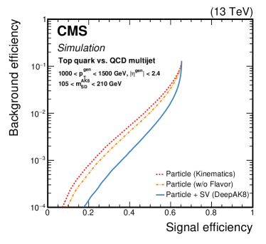
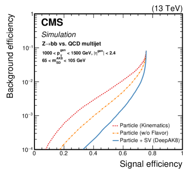
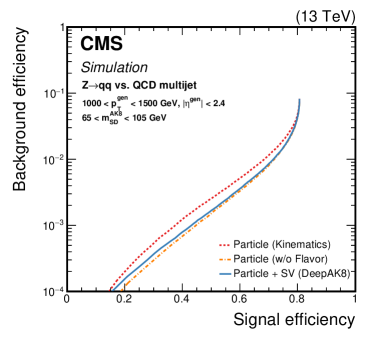
Figure 15: Alternative versions of DeepAK8 trained using a subset of the input features. The details about each version are discussed in the text. The performances of the three versions of DeepAK8 are compared for quark (upper) and boson (lower) identification. For the latter, the left plot corresponds to bosons decaying to a pair of quarks, and the right plot to a pair of light-flavor quarks.

0.7.1 Robustness of tagging algorithms

In addition to the performance of the algorithms in pure discrimination, an important ingredient is their robustness to changes in jet kinematics and data-taking conditions. To quantify this, we study the $\epsilon_{\mathrm{S}}$ and $\epsilon_{\mathrm{B}}$ of the algorithms as a function of the  of the generated particle and the number of reconstructed vertices ($N_{\mathrm{PV}}$) in the event. For these studies, a common working point is defined, corresponding to $\epsilon_{\mathrm{S}}=30$ (50)% for quark (//boson) with $500<\pt(\text{generated particle})<600\GeV$. Working points used in CMS analyses vary from analysis to analysis, since they are optimized to achieve the best sensitivity for the targeted signal processes. For example, CMS employs a quark tagging working point at approximately 40% signal efficiency in the search for BSM production [56], a tagging working point at approximately 20% signal efficiency in the search for BSM diboson production [66], and an tagging working point at approximately 30% signal efficiency in the search for boson pair production [99].

The distributions of the $\epsilon_{\mathrm{S}}$ and $\epsilon_{\mathrm{B}}$ as a function of  of the generated particle for the different particle identification scenarios are displayed in Figs. 16 and 17, respectively. In the low-range for the tagging case, the $\epsilon_{\mathrm{S}}$ for the algorithms using AK8 jets increases rapidly until $\pt\gtrsim 600\GeV$, where a large fraction of jets contain all the decay products. As expected, the $N_{3}\text{-}\mathrm{BDT}\,(\mathrm{CA}15)$ and HOTVR algorithms have a stable $\epsilon_{\mathrm{S}}$ as a function of the generator-level particle . Similar behavior is observed for the quark misidentification rate.

In the case of the and boson tagging, the $\epsilon_{\mathrm{S}}$ for the $m_{\text{SD}}+{\tau_{21}}$ algorithm decreases as a function of $\pt(\text{generated particle})$, whereas the BEST, DeepAK8, and DeepAK8-MD algorithms exhibit improvements in $\epsilon_{\mathrm{S}}$ as a function of $\pt(\text{generated particle})$. The drop in $\epsilon_{\mathrm{S}}$ for $m_{\text{SD}}+{\tau_{21}}$ is a result of the correlation between $m_{\text{SD}}+{\tau_{21}}$ and the jet , leading to a shift in the jet mass distribution to higher values. The $m_{\mathrm{SD}}+N_{2}$ algorithm shows similar behavior to BEST and DeepAK8 algorithms, whereas the $\epsilon_{\mathrm{S}}$ in the case of $m_{\mathrm{SD}}+N_{2}^{\mathrm{DDT}}$ is stable as a function of $\pt(\text{generated particle})$. In contrast to $N$-subjettiness, the ECF observable uses an axis-free approach, which is more efficient in the case of highly collimated decay products.

The misidentification rate has a nontrivial behavior for most algorithms. In the case of DeepAK8 and DeepAK8-MD the $\epsilon_{\mathrm{B}}$ value decreases with $\pt(\text{generated particle})$, which is mainly a result of the use of low-level features as inputs to the algorithm. For $m_{\mathrm{SD}}+N_{2}$, the $\epsilon_{\mathrm{B}}$ increases with $\pt(\text{generated particle})$, whereas for $m_{\mathrm{SD}}+N_{2}^{\mathrm{DDT}}$, it is, by design, significantly more stable. In the case of $m_{\text{SD}}+{\tau_{21}}$, the decrease of $\epsilon_{\mathrm{B}}$ as a function of $\pt(\text{generated particle})$ is mainly caused by the strong shift of the $m_{\mathrm{SD}}$ shape of the background jets to larger values as a result of the selection on $\tau_{21}$. This will be discussed in more detail in Section 0.7.2. Finally, for the BEST, the $\epsilon_{\mathrm{B}}$ decreases up to $\pt(\text{generated particle})\sim 1000\GeV$, and then increases again. This is a feature of the training of the BEST algorithm, stemming from an imbalance in the relative fraction of jets between the low- and high-regimes.

In the case of tagging, the BEST and DeepAK8 algorithms have stable $\epsilon_{\mathrm{S}}$ for $\pt(\text{generated particle})\gtrsim 600\GeV$, whereas for the double-algorithm the $\epsilon_{\mathrm{S}}$ starts to decrease around this regime. There are two main reasons for this behavior. First, the double-algorithm exploits axis-dependent observables, similar to $\tau_{21}$, which are less efficient at high where the decay products become highly collimated. Second, the selection on the tracks used to construct the variables used for the training of the double-algorithm, discussed in Section 0.6.4, is suboptimal in the very high-regime. The efficiency $\epsilon_{\mathrm{B}}$ for both double-and DeepAK8 decreases as a function of $\pt(\text{generated particle})$, whereas for BEST it shows a modest increase for $\pt(\text{generated particle})\gtrsim 1000\GeV$, for the same reasons as in the and boson tagging case.

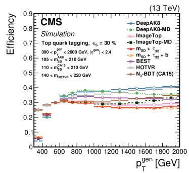
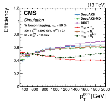
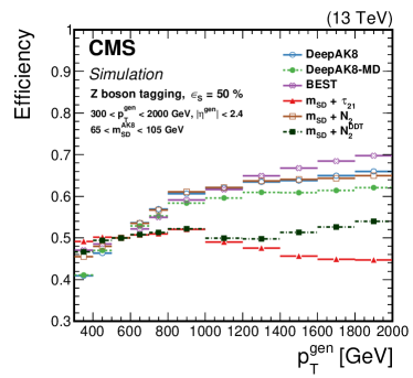
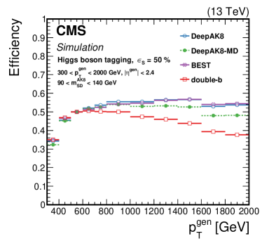
Figure 16: The efficiency $\epsilon_{\mathrm{S}}$ as a function of the generated particle for a working point corresponding to $\epsilon_{\mathrm{S}}=30\,(50)$% for  quark (//boson) identification. Upper left:  quark, upper right:  boson, lower left:  boson, lower right: boson. The error bars represent the statistical uncertainty in each specific bin, due to the limited number of simulated events. Additional fiducial selection criteria applied to the jets are listed in the plots.

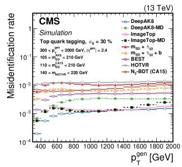
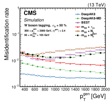
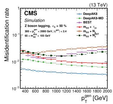
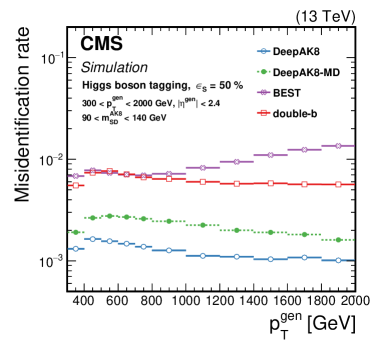
Figure 17: The distribution of $\epsilon_{\mathrm{B}}$ as a function of the generated particle for a working point corresponding to $\epsilon_{\mathrm{S}}=30\,(50)$% for  quark (//boson) identification. Upper left:  quark, upper right:  boson, lower left:  boson, lower right: boson. The error bars represent the statistical uncertainty in each specific bin, due to the limited number of simulated events. Additional fiducial selection criteria applied to the jets are listed in the plots.

The dependence of the algorithms on $N_{\mathrm{PV}}$ is also examined using simulated events. Figure 18 shows the distribution of $\epsilon_{\mathrm{S}}$, and Fig. 19 that of $\epsilon_{\mathrm{B}}$, as a function of $N_{\mathrm{PV}}$ for generated particles with $500<\pt<1000\GeV$, operating at a working point with $\epsilon_{\mathrm{S}}=30$ ($50$)% for quark (//boson) identification as defined above. The algorithms make use of jets that employ PUPPI for pileup mitigation, which results in a roughly constant $\epsilon_{\mathrm{S}}$ and $\epsilon_{\mathrm{B}}$ for all different pileup scenarios.

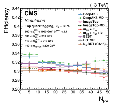
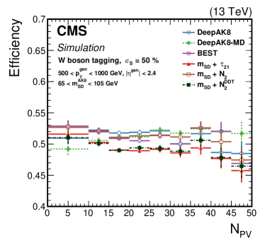
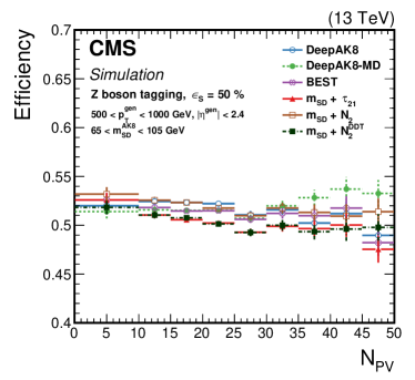
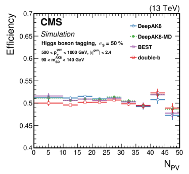
Figure 18: The efficiency $\epsilon_{\mathrm{S}}$ as a function of the number of primary vertices ($N_{\mathrm{PV}}$) for generated particles with $500<\pt<1000\GeV$ at a working point corresponding to $\epsilon_{\mathrm{S}}=30\,(50)$% for  quark (//boson) identification. Upper left:  quark, upper right:  boson, lower left:  boson, lower right: boson. The error bars represent the statistical uncertainty in each specific bin, due to a limited number of simulated events. Additional fiducial selection criteria applied to the jets are listed in the plots.

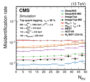
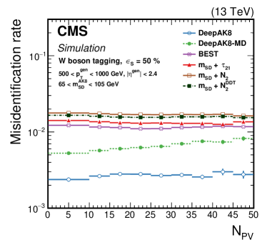
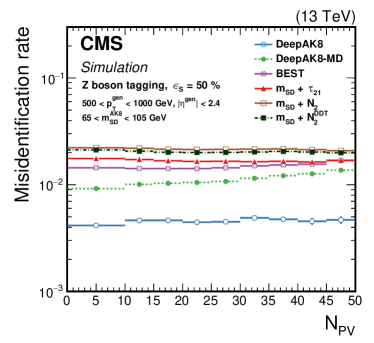
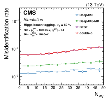
Figure 19: The efficiency $\epsilon_{\mathrm{B}}$ as a function of the number of primary vertices ($N_{\mathrm{PV}}$) for generated particles with $500<\pt<1000\GeV$ at a working point corresponding to $\epsilon_{\mathrm{S}}=30\,(50)$% for  quark (//boson) identification. Upper left:  quark, upper right:  boson, lower left:  boson, lower right: boson. The error bars represent the statistical uncertainty in each specific bin, due to the limited number of simulated events. Additional fiducial selection criteria applied to the jets are listed in the plots.

0.7.2 Correlation with jet mass

A set of studies was performed to understand the correlation of the algorithms with the jet mass. This understanding benefits from the theoretical progress made in jet substructure studies [3], which can result in reduced systematic uncertainties [15]. The jet mass is one of the most discriminating variables, and many analyses require a smoothly falling background jet mass spectrum under a signal peak (e.g., in Ref. [100]). Figure 20 displays the normalized $m_{\mathrm{SD}}$  distribution for jets obtained from the QCD multijet sample, inclusively and after applying a selection with each algorithm. The working point chosen corresponds to $\epsilon_{\mathrm{S}}=30$ ($50$)% for  quark (//boson). The results are shown for one region of the generated particle distribution, but similar behavior is seen for other  regions as well. By design, the BEST and the nominal version of the DeepAK8 algorithms lead to significant sculpting of the background jet mass shape, but this does not affect analyses unless the jet mass distribution is explicitly used in signal extraction, e.g., Ref. [101]. An alternative way of presenting the sculpting of the background jet mass introduced by each tagging algorithm is displayed in Fig. 21. The figure shows the normalized ratio of the background jet mass distributions for the passing and failing jets for each algorithm, after selecting a working point corresponding to $\epsilon_{\mathrm{S}}=30$ (50)% for  quark (//boson). For the mass decorrelated versions of the algorithms, the ratio typically shows very little dependence on $m_{\mathrm{SD}}$.

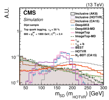
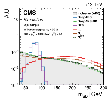
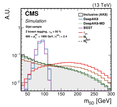
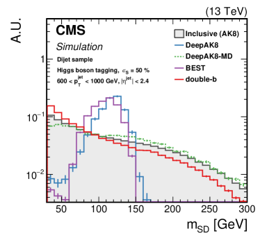
Figure 20: The normalized $m_{\mathrm{SD}}$  distribution for background QCD jets with $600<\pt<1000\GeV$, inclusively and after selection by each algorithm. The working point chosen corresponds to $\epsilon_{\mathrm{S}}=30$ ($\epsilon_{\mathrm{S}}=50$)% for  quark (//boson) identification. Upper left:  quark, upper right:  boson, lower left:  boson, lower right: boson. The error bars represent the statistical uncertainty in each specific bin, which is related to the limited number of simulated events. Additional fiducial selection criteria applied to the jets are listed on the plots.

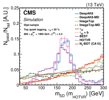
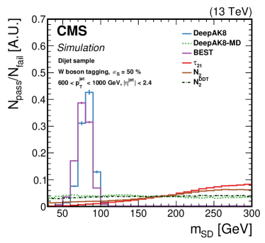
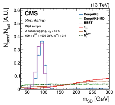
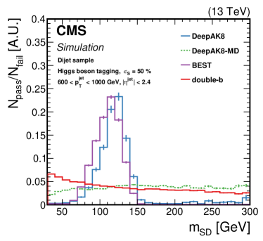
Figure 21: Normalized ratio of the QCD background jet mass distribution for the passing and failing jets with $600<\pt<1000\GeV$, by each algorithm. The working point chosen corresponds to $\epsilon_{\mathrm{S}}=30$ ($\epsilon_{\mathrm{S}}=50$)% for  quark (//boson) identification. Upper left:  quark, upper right:  boson, lower left:  boson, lower right: boson. The error bars represent the statistical uncertainty in each specific bin, which is related to the limited number of simulated events. Additional fiducial selection criteria applied to the jets are listed on the plots.

To quantify the level of mass sculpting we use the Jensen–Shannon divergence (JSD) [102], which is a symmetrized version of the Kullback–Leibler divergence (KLD) [103], and provides a metric for the similarity of the shape between distributions. The KLD is defined as:

$$\text{KLD}(P||Q)=\sum_{i}P(i)\text{log}_{10}\frac{P(i)}{Q(i)},$$ (14)

where $P(i)$ and $Q(i)$ are the normalized mass distributions of the background jets that fail and pass a selection with a given algorithm, respectively, and the symbol $||$ represents the divergence of $P$ from $Q$. The index $i$ runs over the bins of the distributions.

The JSD metric is defined as:

$$\text{JSD}(P||Q)=\frac{1}{2}(\text{KLD}(P||M))+\text{KLD}(Q||M)),~{}~{}\text{where}~{}~{}M=\frac{P+Q}{2}.$$ (15)

Lower values of JSD indicate larger similarity between the mass distributions of jets passing and failing a selection on a given algorithm.

In our studies, the jet mass distributions lay between 30 and 300with a bin size of 10. The JSD values for successively tighter selections (expressed in terms of decreasing $\epsilon_{\mathrm{B}}$) for the various quark and boson tagging algorithms are shown in Fig. 22. The best decorrelation for the tagging cases is achieved with the DeepAK8-MD algorithm, which exploits an adversarial network to reduce the correlation of the tagging score with the jet mass. For tagging, $m_{\mathrm{SD}}+N_{2}^{\mathrm{DDT}}$ and DeepAK8-MD achieve similar levels of mass decorrelation. As expected, tighter selection on the tagging score results in an increase of the mass sculpting. A similar behavior is observed for all algorithms.

The robustness of the mass decorrelation techniques is further studied as a function of jet and $N_{\mathrm{PV}}$. These studies are performed for a working point corresponding to $\epsilon_{\mathrm{S}}=30$ (50)% for () tagging. Figure 23 shows the JSD values as a function of the jet for jets from QCD multijet events. Most algorithms show modest dependence on jet , except for ImageTop-MD, where the mass dependence increases rapidly when $\pt\lesssim 600\GeV$ as the training was only performed for jets with $\pt>600\GeV$. The DeepAK8-MD and $m_{\mathrm{SD}}+N_{2}^{\mathrm{DDT}}$ algorithms for tagging also show modestly increased mass dependence in the range of 1200 and $1600\GeV$, respectively. The dependence of the mass mitigation techniques on $N_{\mathrm{PV}}$ was also studied and was small.

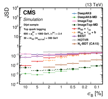
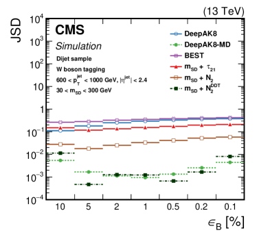
Figure 22: The JSD as a function of successively tighter selections (expressed in terms of $\epsilon_{\mathrm{B}}$) for the various (left) and (right) tagging algorithms. Lower values of JSD indicate larger similarity of the m_SD in QCD multijet events passing and failing the selection on the tagging algorithm. Additional fiducial selection criteria applied to the jets are listed in the plots.

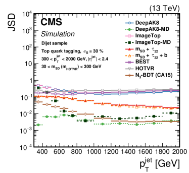
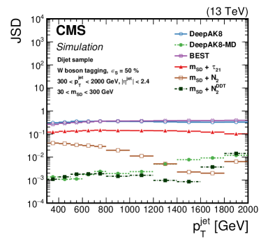
Figure 23: The JSD, as a function of the jet for the various (left) and (right) tagging algorithms. Lower values of JSD indicate larger similarity of the m_SD in QCD multijet events passing and failing the selection on the tagging algorithm. Additional fiducial selection criteria applied to the jets are listed in the plots.

0.8 Performance in data and systematic uncertainties

In this section, the validation of the algorithms using data is presented. The validation is performed in two steps. In the first step, we focus on studying the overall modeling of key variables in simulation and their agreement with data, as well as the dependence on the simulation details. The second step is to use these results to extract corrections to the simulation so that the algorithms perform similarly in simulation and data. Differences in the performance between data and simulation are corrected by scale factors (SF) extracted by comparing the efficiencies in data and simulation. To account for effects not captured in the SF, multiple sources of systematic uncertainties are considered. The data and simulated samples used for these studies are described in Section 0.5.

In this paper, we focus on the calibration of the quark and /boson tagging algorithms. The calibration of tagging algorithms where and bosons decay to a pair of bottom or charm quarks requires alternative methods that go beyond the scope of this paper. Since it is challenging to obtain a pure or boson sample, the calibration of such taggers relies on the use of a proxy jet, i.e., a jet obtained in the dijet sample with characteristics similar to signal jets. Data-to-simulation correction factors are extracted based on these proxy jets, which are then applied to signal jets. Therefore, the proxy jets should be selected to have similar characteristics to the signal jets. To this end, jets arising from gluon splitting to $\bbbar$ or $\ccbar$ are used as proxy jets from a sample dominated by QCD multijet events. Such approaches have been followed in Refs. [81, 20, 104].

0.8.1 Systematic uncertainties

A number of sources of systematic effects can affect the modeling of the performance of the algorithms in data by the simulation. These include systematic uncertainties in the parton showering model, renormalization and factorization scales, PDFs, jet energy scale and resolution, unclustered energy, trigger and lepton identification, pileup modeling, and integrated luminosity, as well as statistical uncertainties of simulated samples.

Parton shower uncertainties for signal jets are evaluated using samples with the same event generators but a different choice for the modeling of the parton showering. For background jets, a sample produced using an alternative generator for both the hard scattering and the parton shower is used. The details of the samples are discussed in Section 0.3. Changes in renormalization ($\mu_{R}$) and factorization ($\mu_{F}$) scales are estimated by varying the scales separately by a factor of two up and down, relative to the choices of the scale values used in the sample generation. The uncertainty related to the choice of the PDFs is obtained from the standard deviation in 100 replicas of the NNPDF3.0 PDF set [31]. The jet energy scale and resolution are changed within their $\pt$- and $\eta$-dependent uncertainties, based on the studies presented in Ref. [51]. Their effects are also propagated to . The effect of the uncertainty in the measurement of the unclustered energy (i.e., contribution of PF candidates not associated to any of the physics objects) is evaluated based on the momentum resolution of each PF candidate, which depends on the type of the candidate [52]. Uncertainties in the measurement of the trigger efficiency and in the energy/momentum scale and resolution of the leptons are propagated in the SF extraction. The uncertainty in the pileup weighting procedure is determined by varying the minimum bias cross section used to produce the pileup profile by $\pm$5% from the measured central value of 69.2 mb [105, 106]. The limited size of the simulated samples and the size of the data control samples are also considered.

The uncertainties described above contribute in different ways to the modeling of jet kinematics and the extraction of SF. Because many of the algorithms detailed in this paper use jet substructure and jet constituent information, either directly or as input to multivariate techniques, the uncertainties in the choice of parton shower are significant. Different parton showers directly affect the number, momentum, and distribution of jet constituents, influencing the observables used as inputs to the multivariate techniques, and eventually propagating to the outputs of those algorithms. The magnitude of this source of systematic uncertainty is from 10–30%. The uncertainty in the value of $\mu_{R}$ and $\mu_{F}$ chosen for event generation also has a sizable impact (5–15%), because this changes the amount of radiation that can enter into a reconstructed jet. These dominant components contribute a total combined uncertainty of 10–50%, depending on the specific jet kinematics of interest.

Additional sources of systematic uncertainties, with smaller impact, are also considered. For example, the trigger and lepton identification uncertainties are a few percent, and do not include uncertainties in the kinematic distributions. The identification of leptons, especially muons, is nearly fully efficient, and the trigger is selected to ensure full efficiency in the regime of interest. The jet energy scale and resolution uncertainties are similar, including shape components, and are between 1 and 5% for the high-jets studied here. Uncertainties related to pileup modeling and the integrated luminosity measurement have an effect smaller than $3\%$.

These uncertainties partially cancel in the SF measurement, as will be discussed in Section 0.8.4.

0.8.2 The quark and boson identification performance in data

The single-$\mu$ event selection discussed in Section 0.5.1 provides a sample dominated by semileptonic events. One of the  quarks decays to a b̃oson that decays leptonically (to pass the selection), and the other provides a hadronic decay to be used in validating the algorithms.

To study possible dependence of the tagging efficiency on the parton showering scheme, we consider two alternative simulated  samples. As discussed in Section 0.3, both samples are generated with the same generator (i.e., ), but one uses for the modeling of the parton showering, whereas the other uses . The total SM expectation from simulation using the latter sample will be referred to as “SM (Herwig)”. As we will see, the choice of the parton showering generator has only a small impact on the overall agreement between data and simulation in signal jets.

To account for the differences in the design of the algorithms, the large-$R$ jets discussed in Section 0.5.1 are either AK8, CA15, or HOTVR jets. For brevity we focus mainly on results using AK8 jets, unless otherwise stated, but similar conclusions can be drawn from all three jet collections.

The data-to-simulation comparisons of basic jet kinematic and substructure variables: $\pt(\text{jet})$, $m_{\mathrm{SD}}$, the $N$-subjettiness ratios $\tau_{32}$ and $\tau_{21}$, and the $N_{2}$ and $N_{2}^{\mathrm{DDT}}$, are shown in Fig. 24. Figure 25 displays the main observables of the HOTVR algorithm, $m_{\text{HOTVR}}$, $m_{\text{min,HOTVR}}$ and $N_{\text{sub,HOTVR}}$, in data and simulation. The next set of comparisons includes tagging algorithms that are based on high-level jet substructure observables and explore ML techniques to improve performance, namely the BEST and the $N_{3}\text{-}\mathrm{BDT}\,(\mathrm{CA}15)$ algorithms. Figure 26 shows the  quark and boson identification probabilities of BEST and the tagging discriminant for the $N_{3}\text{-}\mathrm{BDT}\,(\mathrm{CA}15)$, in data and simulation. The last set of comparisons is related to the ImageTop and the DeepAK8 algorithms, which both explore lower-level observables. Figure 27 displays the distributions of the  quark identification probability for the two versions of ImageTop, and the  quark and boson identification probabilities for DeepAK8 algorithms.

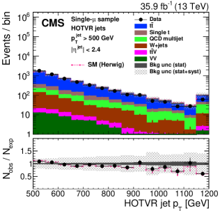
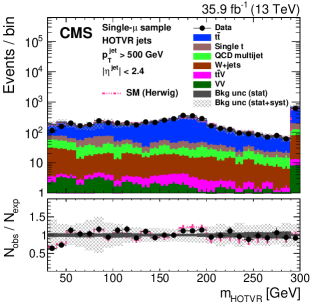
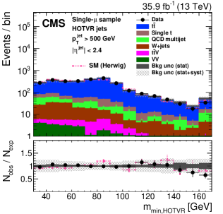
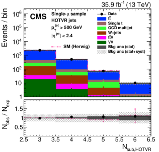
Figure 29: Distribution of the main observables of the HOTVR algorithm, HOTVR jet (upper left), $m_{\text{HOTVR}}$ (upper right), $m_{\text{min,HOTVR}}$ (lower left) and $N_{\text{sub,HOTVR}}$ (lower right) in data and simulation in the single-$\mu$ signal sample, after applying a jet momentum cut $\pt>500\GeV$. The pink line corresponds to the simulation distribution obtained using the alternative sample. The background event yield is normalized to the total observed data yield. The lower panel shows the data to simulation ratio. The solid dark-gray (shaded light-gray) band corresponds to the total uncertainty (statistical uncertainty of the simulated samples), the pink line to the data to simulation ratio using the alternative sample, and the vertical black lines correspond to the statistical uncertainty of the data. The vertical pink lines correspond to the statistical uncertainty of the alternative sample. The distributions are weighted according to the top quark weighting procedure described in the text.

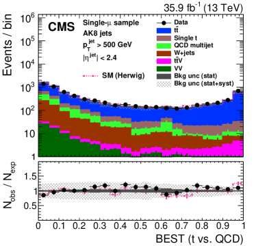
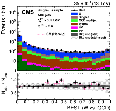
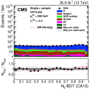
Figure 30: Distribution of the  quark (upper left) and  boson (upper right) identification probabilities for the BEST algorithm, and the $N_{3}\text{-}\mathrm{BDT}\,(\mathrm{CA}15)$ discriminant in data and simulation in the single-$\mu$ signal sample, after applying a jet momentum cut $\pt>500\GeV$. The pink line corresponds to the simulation distribution obtained using the alternative sample. The background event yield is normalized to the total observed data yield. The lower panel shows the data to simulation ratio. The solid dark-gray (shaded light-gray) band corresponds to the total uncertainty (statistical uncertainty of the simulated samples), the pink line to the data to simulation ratio using the alternative sample, and the vertical black lines correspond to the statistical uncertainty of the data. The vertical pink lines correspond to the statistical uncertainty of the alternative sample. The distributions are weighted according to the top quark weighting procedure described in the text.

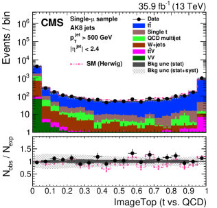
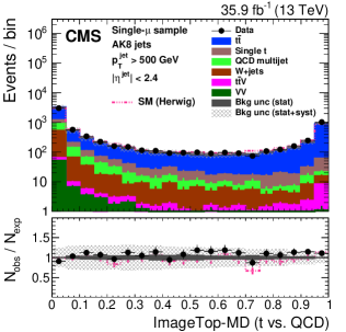
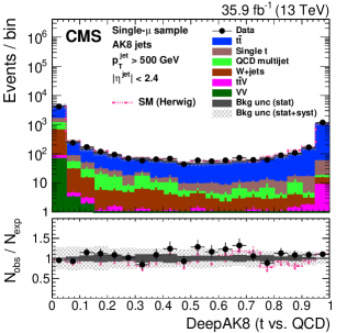
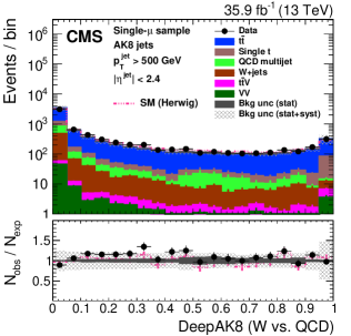
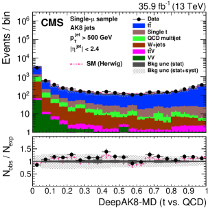
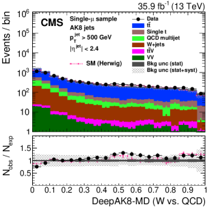
Figure 31: Distribution of the ImageTop (upper left) and ImageTop-MD (upper right) discriminant in data and simulation in the single-$\mu$ sample. The plots in the middle row show the  quark (left) and  boson (right) identification probabilities in data and simulation for the DeepAK8 algorithm after applying a jet momentum cut $\pt>500\GeV$. The corresponding plots for DeepAK8-MD are displayed in the lower row. The pink line corresponds to the simulation distribution obtained using the alternative sample. The background event yield is normalized to the total observed data yield. The lower panel shows the data to simulation ratio. The solid dark-gray (shaded light-gray) band corresponds to the total uncertainty (statistical uncertainty of the simulated samples), the pink line to the data to simulation ratio using the alternative sample, and the vertical black lines correspond to the statistical uncertainty of the data. The vertical pink lines correspond to the statistical uncertainty of the alternative sample. The distributions are weighted according to the top quark weighting procedure described in the text.

Because the selection applied to events shown in Figs. 24–27 results in a sample with low purity of fully merged quark decay products, we also study the same distributions after applying a tighter requirement on the jet momenta: $\pt>500\GeV$. This selection results in a sample consisting of a higher fraction of fully merged quark jets, relative to the jet component from the decay of a boosted boson jet. Figures 28-31 show the same distributions for this high-selection.

The total background yield is normalized to the observed number of data events. The systematic uncertainties discussed in Section 0.8.1 are also considered and are shown via the shaded dark-grey band in the figures. Overall, the shapes in data are compatible with the expectation from simulation within uncertainties for all the algorithms.

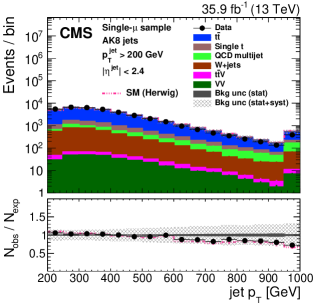
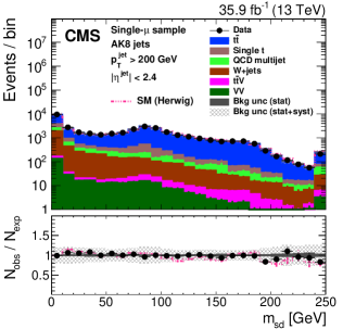
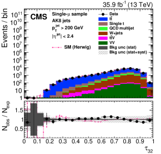
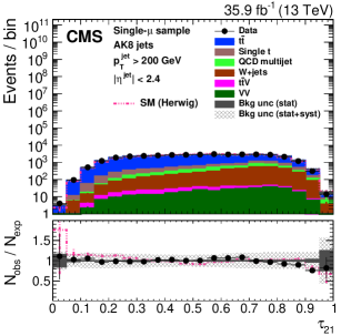
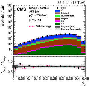
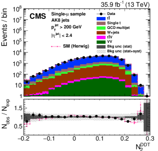
Figure 24: Distribution of the jet (upper left), jet mass, $m_{\mathrm{SD}}$  (upper right), the $N$-subjettiness ratios $\tau_{32}$ (middle left) and $\tau_{21}$ (middle right), and the $N_{2}$ (lower left) and $N_{2}^{\text{DDT}}$ (lower right) in data and simulation in the single-$\mu$ signal sample. The pink line corresponds to the simulation distribution obtained using the alternative sample. The background event yield is normalized to the total observed data yield. The lower panel shows the data to simulation ratio. The solid dark-gray (shaded light-gray) band corresponds to the total uncertainty (statistical uncertainty of the simulated samples), the pink line to the data to simulation ratio using the alternative sample, and the vertical black lines correspond to the statistical uncertainty of the data. The vertical pink lines correspond to the statistical uncertainty of the alternative sample. The distributions are weighted according to the top quark weighting procedure described in the text.

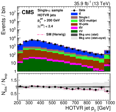
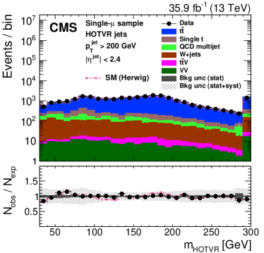
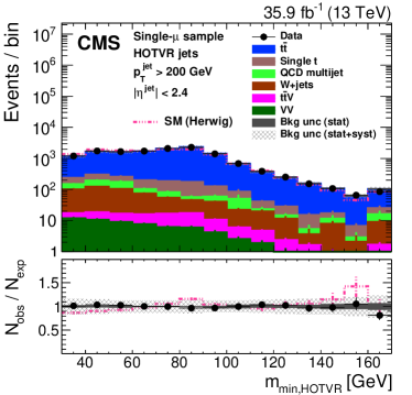
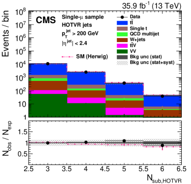
Figure 25: Distribution of the main observables of the HOTVR algorithm, HOTVR jet (upper left), $m_{\text{HOTVR}}$ (upper right), $m_{\text{min,HOTVR}}$ (lower left), and $N_{\text{sub,HOTVR}}$ (lower right) in data and simulation in the single-$\mu$ signal sample. The pink line corresponds to the simulation distribution obtained using the alternative sample. The background event yield is normalized to the total observed data yield. The lower panel shows the data to simulation ratio. The solid dark-gray (shaded light-gray) band corresponds to the total uncertainty (statistical uncertainty of the simulated samples), the pink line to the data to simulation ratio using the alternative sample, and the vertical black lines correspond to the statistical uncertainty of the data. The vertical pink lines correspond to the statistical uncertainty of the alternative sample. The distributions are weighted according to the top quark weighting procedure described in the text.

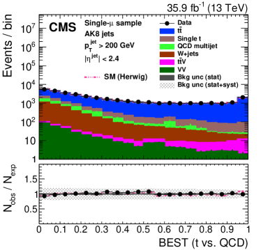
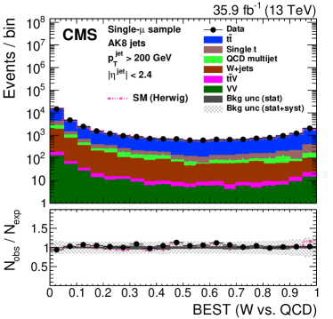
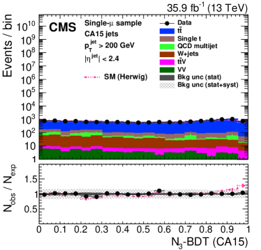
Figure 26: Distribution of the  quark (upper left) and  boson (upper right) identification probabilities for the BEST algorithm, and the $N_{3}\text{-}\mathrm{BDT}\,(\mathrm{CA}15)$ discriminant in data and simulation in the single-$\mu$ signal sample. The pink line corresponds to the simulation distribution obtained using the alternative sample. The background event yield is normalized to the total observed data yield. The lower panel shows the data to simulation ratio. The solid dark-gray (shaded light-gray) band corresponds to the total uncertainty (statistical uncertainty of the simulated samples), the pink line to the data to simulation ratio using the alternative sample, and the vertical black lines correspond to the statistical uncertainty of the data. The vertical pink lines correspond to the statistical uncertainty of the alternative sample. The distributions are weighted according to the top quark weighting procedure described in the text.

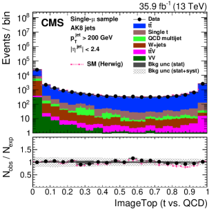
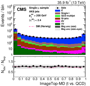
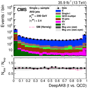
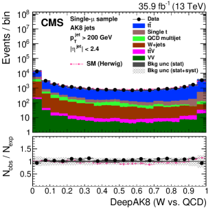
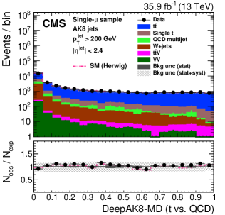
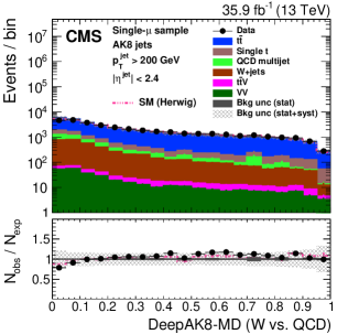
Figure 27: Distribution of the ImageTop (upper left) and ImageTop-MD (upper right) discriminant in data and simulation in the single-$\mu$ sample. The plots in the middle row show the  quark (left) and  boson (right) identification probabilities in data and simulation for the DeepAK8 algorithm. The corresponding plots for DeepAK8-MD are displayed in the lower row. The pink line corresponds to the simulation distribution obtained using the alternative sample. The background event yield is normalized to the total observed data yield. The lower panel shows the data to simulation ratio. The solid dark-gray (shaded light-gray) band corresponds to the total uncertainty (statistical uncertainty of the simulated samples), the pink line to the data to simulation ratio using the alternative sample, and the vertical black lines correspond to the statistical uncertainty of the data. The vertical pink lines correspond to the statistical uncertainty of the alternative sample. The distributions are weighted according to the top quark weighting procedure described in the text.

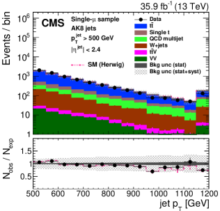
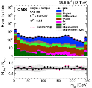
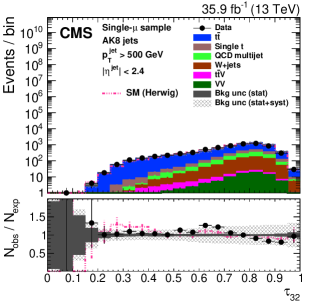
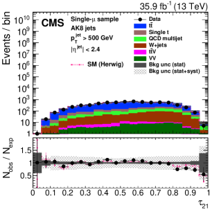
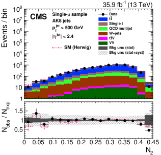
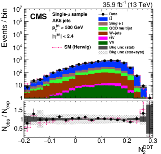
Figure 28: Distribution of the jet (upper left), the jet mass, $m_{\mathrm{SD}}$ (upper right), the $N$-subjettiness ratios $\tau_{32}$ (middle left) and $\tau_{21}$ (middle right), and the $N_{2}$ (lower left) and $N_{2}^{\text{DDT}}$ (lower right) in data and simulation in the single-$\mu$ signal sample after applying a jet momentum cut $\pt>500\GeV$. The pink line corresponds to the simulation distribution obtained using the alternative sample. The background event yield is normalized to the total observed data yield. The lower panel shows the data to simulation ratio. The solid dark-gray (shaded light-gray) band corresponds to the total uncertainty (statistical uncertainty of the simulated samples), the pink line to the data to simulation ratio using the alternative sample, and the vertical black lines correspond to the statistical uncertainty of the data. The vertical pink lines correspond to the statistical uncertainty of the alternative sample. The distributions are weighted according to the top quark weighting procedure described in the text.

0.8.3 Misidentification probability in data

The misidentification probability of the algorithms is studied in the dijet and single-$\gamma$ data samples. The two samples differ in the relative fraction of light-flavor quarks and gluons in the final state. To study the dependence of the misidentification probability on the choice of the event generator and the parton showering scheme, we consider two different simulated samples to model the QCD multijet background. The nominal sample uses for the event generation and (P8) for the parton showering and hadronization, whereas the alternative sample uses for event generation and the modeling of the parton showering. More information on the generation of these samples is discussed in Section 0.3. The total SM contribution estimated using the QCD multijet sample is referred to as “SM (Herwig)”. As in Section 0.8.2, we will focus on results using jets with $R=0.8$, unless otherwise stated. To account for possible differences in the distribution of the QCD multijet and $\gamma+$jet simulated events, the total background yield is weighted to match the distribution in data, following the procedure discussed in Section 0.3.

The distributions of $m_{\mathrm{SD}}$, jet , the $N$-subjettiness ratios $\tau_{32}$ and $\tau_{21}$, and the $N_{2}$ and $N_{2}^{\text{DDT}}$, in the dijet sample are displayed in Fig. 32. For this event selection, the shapes of the $m_{\mathrm{SD}}$ and the $N$-subjettiness ratios are described well by simulation, whereas there is disagreement between data and simulation for high values of $N_{2}$ and $N_{2}^{\text{DDT}}$. A better description of the data, particularly for $N_{2}^{\text{DDT}}$, is achieved with the QCD multijet sample, which hints that the disagreement is related to the description of the parton shower. For the other observables we observe similar level of agreement between the two generators.

The same set of variables is presented in Fig. 33 for the single-$\gamma$ sample. From previous measurements [8], the $m_{\mathrm{SD}}$ agrees very well with simulation except at low masses. The modeling of the $N$-subjettiness and $N_{2}$ ratios is poorer in the single-$\gamma$ sample.

Figures 34 and 35 show the distribution of the main observables of the HOTVR algorithm, namely $m_{\text{HOTVR}}$, $m_{\text{min,HOTVR}}$, and $N_{\text{sub,HOTVR}}$, in data and simulation, in the dijet and single-$\gamma$ samples, respectively. In both samples, $m_{\text{HOTVR}}$ and $m_{\text{min,HOTVR}}$ show good agreement between data and simulation. The $N_{\text{sub,HOTVR}}$ distribution in data is softer than in simulation. Similar conclusions hold using to simulate the QCD multijet events. The difference is more pronounced in the single-$\gamma$ sample. The $N_{\text{sub,HOTVR}}$ is particularly sensitive to the precise modeling of the parton showering.

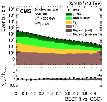
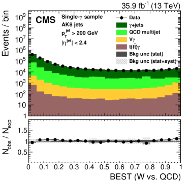
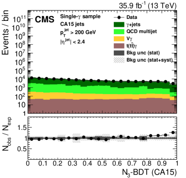
Figure 37: Distribution of the  quark (upper left) and  boson (upper right) identification probabilities for the BEST algorithm, and the $N_{3}\text{-}\mathrm{BDT}\,(\mathrm{CA}15)$ discriminant in data and simulation in the single-$\gamma$ sample. The background event yield is normalized to the total observed data yield. The background event yield is normalized to the total observed data yield. The lower panel shows the data to simulation ratio. The solid dark-gray (shaded light-gray) band corresponds to the total uncertainty (statistical uncertainty of the simulated samples), and the vertical lines correspond to the statistical uncertainty of the data. The distributions are weighted so that the jet distribution of the simulation matches the data.

The distribution of the quark and boson identification probabilities for BEST and the quark tagging discriminant for the $N_{3}\text{-}\mathrm{BDT}\,(\mathrm{CA}15)$ algorithm in the dijet sample are presented in Fig. 36, and the equivalent plots for the single-$\gamma$ selection are shown in Fig. 37. In both samples the agreement between data and simulation is reasonable. Some disagreement is observed in the very high values ($\gtrsim$0.95) for the quark identification probability of the BEST algorithm in the single-$\gamma$ sample. The disagreement is observed in the region of the quark probability greater than 0.95, which is significantly higher than the recommended operating points. Some disagreement is observed between the nominal QCD multijet simulated sample and the alternative sample for large values of the boson probability of the BEST algorithm, with the nominal sample showing better agreement with the data.

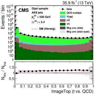
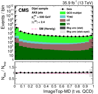
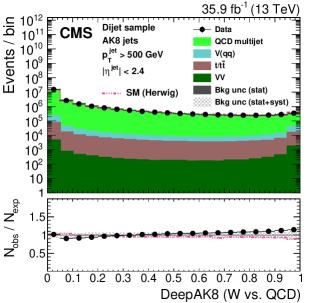
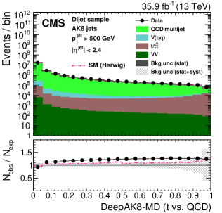
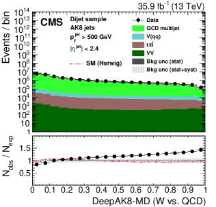
Figure 38: Distribution of the ImageTop (upper left) and ImageTop-MD (upper right) discriminant in data and simulation in the dijet sample. The plots in the middle row show the  quark (left) and  boson (right) identification probabilities in data and simulation for the DeepAK8 algorithm. The corresponding plots for DeepAK8-MD are displayed in the lower row. The pink line corresponds to the simulation distribution obtained using the alternative QCD multijet sample. The background event yield is normalized to the total observed data yield. The lower panel shows the data to simulation ratio. The solid dark-gray (shaded light-gray) band corresponds to the total uncertainty (statistical uncertainty of the simulated samples), the pink line to the data to simulation ratio using the alternative QCD multijet sample, and the vertical black lines correspond to the statistical uncertainty of the data. The vertical pink lines correspond to the statistical uncertainty of the alternative QCD multijet sample. The distributions are weighted so that the jet distribution of the simulation matches the data.

The distributions of the ImageTop and DeepAK8 discriminants are shown in Figs. 38 and 39 for jets in the dijet and single-$\gamma$ samples, respectively. The overall agreement between data and simulation in the single-$\gamma$ is better than in the dijet sample. Moreover, the discrepancy in the shape is mainly observed at the very low values of the discriminant and is more enhanced in the tagging case. The dijet sample is dominated by jets initiated by gluons, especially at low values of the discriminant. In addition, ImageTop and DeepAK8 are very sensitive to mismodeling of quarks or gluons in the simulation, and so exhibit more sample dependence. QCD multijet events simulated using generally show better agreement with the data.

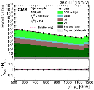
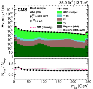
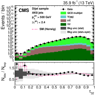
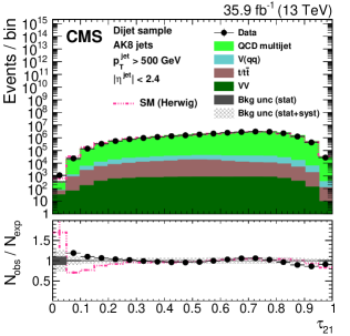
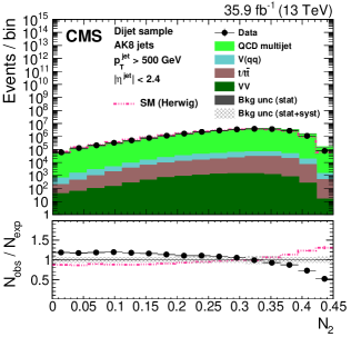
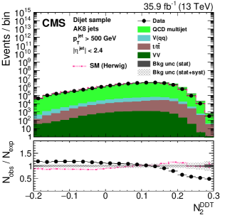
Figure 32: Distribution of the jet (upper left), the jet mass, $m_{\mathrm{SD}}$ (upper right), the $N$-subjettiness ratios $\tau_{32}$ (middle left) and $\tau_{21}$ (middle right), and the $N_{2}$ (lower left) and $N_{2}^{\text{DDT}}$ (lower right) in data and simulation in the dijet sample. The pink line corresponds to the simulation distribution obtained using the alternative QCD multijet sample. The background event yield is normalized to the total observed data yield. The lower panel shows the data to simulation ratio. The solid dark-gray (shaded light-gray) band corresponds to the total uncertainty (statistical uncertainty of the simulated samples), the pink line to the data to simulation ratio using the alternative QCD multijet sample, and the vertical black lines correspond to the statistical uncertainty of the data. The vertical pink lines correspond to the statistical uncertainty of the alternative QCD multijet sample. The distributions are weighted so that the jet distribution of the simulation matches the data.

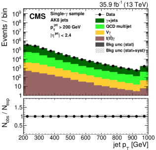
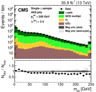
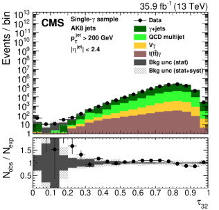
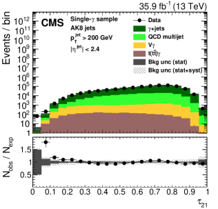
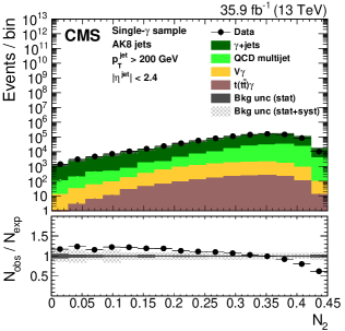
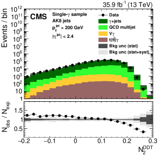
Figure 33: Distribution of the jet  (upper left), the jet mass, $m_{\mathrm{SD}}$ (upper right), the $N$-subjettiness ratios $\tau_{32}$ (middle left) and $\tau_{21}$ (middle right), and the $N_{2}$ (lower left) and $N_{2}^{\text{DDT}}$ (lower right) in data and simulation in the single-$\gamma$ sample. The background event yield is normalized to the total observed data yield. The lower panel shows the data to simulation ratio. The solid dark-gray (shaded light-gray) band corresponds to the total uncertainty (statistical uncertainty of the simulated samples), and the vertical lines correspond to the statistical uncertainty of the data. The distributions are weighted so that the jet distribution of the simulation matches the data.

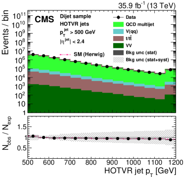
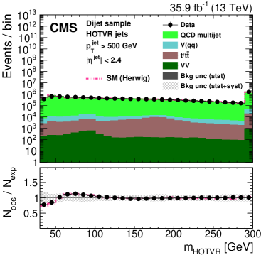
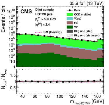
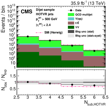
Figure 34: Distribution of the main observables of the HOTVR algorithm, HOTVR jet (upper left), $m_{\text{HOTVR}}$ (upper right), $m_{\text{min,HOTVR}}$ (lower left) and $N_{\text{sub,HOTVR}}$ (lower right) in data and simulation in the dijet sample. The pink line corresponds to the simulation distribution obtained using the alternative QCD multijet sample. The background event yield is normalized to the total observed data yield. The lower panel shows the data to simulation ratio. The solid dark-gray (shaded light-gray) band corresponds to the total uncertainty (statistical uncertainty of the simulated samples), the pink line to the data to simulation ratio using the alternative QCD multijet sample, and the vertical black lines correspond to the statistical uncertainty of the data. The vertical pink lines correspond to the statistical uncertainty of the alternative QCD multijet sample. The distributions are weighted so that the jet distribution of the simulation matches the data.

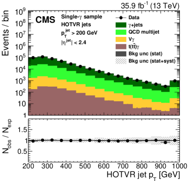
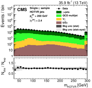
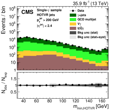
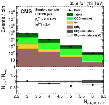
Figure 35: Distribution of the main observables of the HOTVR algorithm, HOTVR jet (upper left), $m_{\text{HOTVR}}$ (upper right), $m_{\text{min,HOTVR}}$ (lower left) and $N_{\text{sub,HOTVR}}$ (lower right) in data and simulation in the single-$\gamma$ sample. The background event yield is normalized to the total observed data yield. The lower panel shows the data to simulation ratio. The solid dark-gray (shaded light-gray) band corresponds to the total uncertainty (statistical uncertainty of the simulated samples), and the vertical lines correspond to the statistical uncertainty of the data. The distributions are weighted so that the jet distribution of the simulation matches the data.

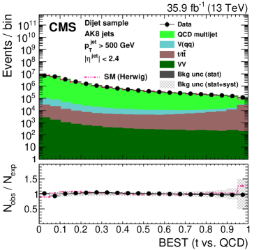
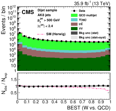
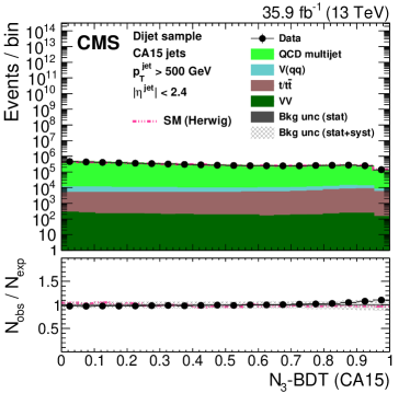
Figure 36: Distribution of the  quark (upper left) and  boson (upper right) identification probabilities for the BEST algorithm, and the $N_{3}\text{-}\mathrm{BDT}\,(\mathrm{CA}15)$ discriminant in data and simulation in the dijet sample. The background event yield is normalized to the total observed data yield. The pink line corresponds to the simulation distribution obtained using the alternative QCD multijet sample. The background event yield is normalized to the total observed data yield. The lower panel shows the data to simulation ratio. The solid dark-gray (shaded light-gray) band corresponds to the total uncertainty (statistical uncertainty of the simulated samples), the pink line to the data to simulation ratio using the alternative QCD multijet sample, and the vertical black lines correspond to the statistical uncertainty of the data. The vertical pink lines correspond to the statistical uncertainty of the alternative QCD multijet sample. The distributions are weighted so that the jet distribution of the simulation matches the data.

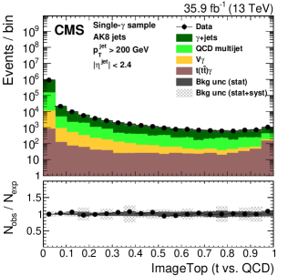
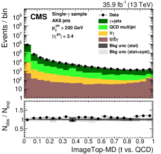
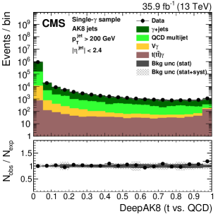
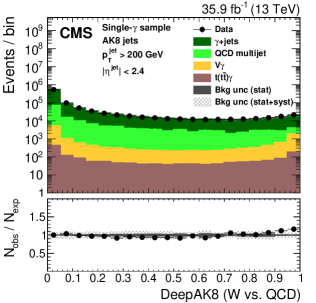
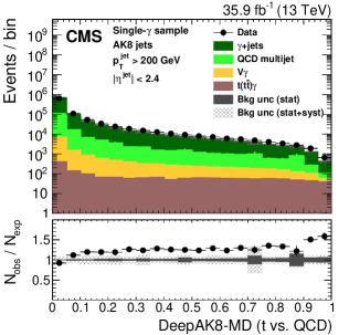
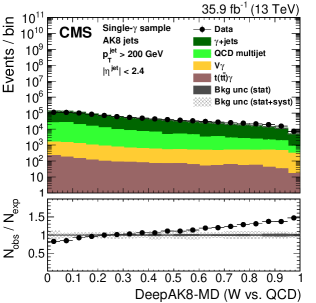
Figure 39: Distribution of the ImageTop (upper left) and ImageTop-MD (upper right) discriminant in data and simulation in the single-$\gamma$ sample. The plots in the middle row show the  quark (left) and  boson (right) identification probabilities in data and simulation for the DeepAK8 algorithm. The corresponding plots for DeepAK8-MD are displayed in the lower row. The background event yield is normalized to the total observed data yield. The lower panel shows the data to simulation ratio. The solid dark-gray (shaded light-gray) band corresponds to the total uncertainty (statistical uncertainty of the simulated samples), and the vertical lines correspond to the statistical uncertainty of the data. The distributions are weighted so that the jet distribution of the simulation matches the data.

0.8.4 Corrections to simulation

The measurement of the  quark and  boson tagging efficiencies in data are performed in the single-$\mu$ sample using a “tag-and-probe” method [107]. The muon, in combination with the -tagged jet, is used as the “tag”. In the opposite hemisphere of the event, the jet is considered as the “probe jet”.

The total SM sample is decomposed into three categories based on the spatial separation of the partons from the  quark decay with respect to the AK8 jet, following the discussion in Section 0.4. The “Merged  quark” category includes cases where the three partons and the jet have $\Delta R<0.6$. The “Merged  boson” category includes cases where only the two partons from the  boson decay are within $\Delta R<0.6$ of the jet and the quark from the top quark decay is outside the jet cone. Any other topology falls in the “Nonmerged” category. In the cases of the HOTVR and $N_{3}\text{-}\mathrm{BDT}\,(\mathrm{CA}15)$ algorithms, the matching requirement is adjusted from 0.6 to 1.2.

The jet mass distributions in simulation of each one of the three categories are used to derive templates to fit the jet mass distribution in data. For a given working point, the fit is done for all three categories simultaneously for both the “passing” and “failing” events. The fit is performed in the range from 50 to 250with a bin width of 10. The sources of systematic uncertainties discussed in Section 0.8.1 are considered and are treated as nuisance parameters in the fit. After calculating the efficiencies in data ($\epsilon_{\text{Data}}$) and simulation ($\epsilon_{\text{Simulation}}$), the SF is determined as the ratio of $\epsilon_{\text{Data}}$ over $\epsilon_{\text{Simulation}}$.

The SFs are extracted differentially in jet for the quark and boson tagging working points discussed in Section 0.7.1. For the case of  quark identification the following exclusive jet regions are considered: 300–400, 400–480, 480–600, and 600–1200. To increase the purity of “Merged  boson” candidates, we consider regions with lower jet : 200–300, 300–400, 400–550, and 550–800. The effects of the systematic sources discussed in Section 0.8.1 are propagated to uncertainties in the SF. The $m_{\mathrm{SD}}$ distributions after performing the maximum likelihood fit for data and simulation in the passing and failing categories for DeepAK8-MD for $400<\pt<480\GeV$ are displayed in Fig. 40.

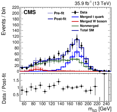
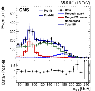
Figure 40: The $m_{\mathrm{SD}}$ distribution in data and simulation in the passing (left) and failing (right) categories for DeepAK8-MD for the jet in the 400–800range. The solid lines correspond to the contribution of each category after performing the maximum likelihood fit as described in the text. The dashed lines are the expectation from simulation before the fit. The lower panel shows the data to simulation ratio. The vertical black lines correspond to the total uncertainty, including the statistical uncertainty of the data, after the fit.

The SFs measured for each of the  quark and  boson identification algorithms are summarized in Fig. 41. The SFs are typically consistent with unity, within the uncertainties. The largest SF is measured for the identification of  quarks using DeepAK8-MD. The statistical and parton shower uncertainties dominate the SF measurement. The algorithms designed to avoid strong dependence on the mass, such as the DeepAK8-MD, have typically smaller uncertainties than the other algorithms. The effect of systematic uncertainties is more pronounced in algorithms that utilize a larger set of observables to increase discrimination power. These algorithms (i.e., BEST, ImageTop, and DeepAK8) are more sensitive to the simulation details. The features are more evident in the boson case, due to the larger sample size of the “Merged  boson” category compared to the “Merged  quark” category, which allows for more precise comparisons due to increased number of events.

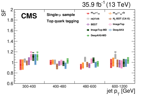
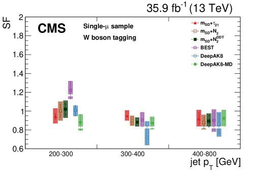
Figure 41: Summary of the scale factors (SF) measured for each of the  quark (upper) and  boson (lower) identification algorithms. The markers correspond to the SF value, the error bars to the statistical uncertainty on the SF measurement, and the band is the total uncertainty, including the systematic component.

The misidentification rate as a function of the jet , is displayed in Figs. 42 and 43 for the and tagging algorithms. To study the dependence of the misidentification probability on the matrix element generator, and on the parton showering, we use an additional simulation sample for the QCD multijet background, which uses for both the hard scattering generation and parton showering. In some cases, the misidentification probabilities show a significant dependence (up to $\sim$25%) on the simulation details, particularly for the ImageTop and DeepAK8 algorithms. The main source of this dependence is the description of gluon content; these are the only algorithms that have access to quark-gluon separation to improve the performance. Differences in the quark/gluon content can have large effects on the uncertainties.

The misidentification probability is also studied in the single-$\gamma$ sample. Overall the performance in data and simulation agrees better in this sample than in the dijet sample. This can be attributed to the fact that the single-$\gamma$ sample has a larger fraction of light-flavor quarks, which are better modeled in simulation [18].

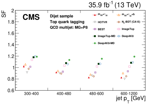
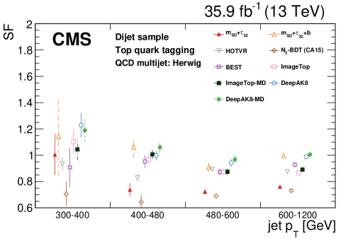
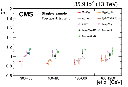
Figure 42: The ratio of the misidentification rate of  quarks in data and simulation in the dijet (upper and middle rows) and the single-$\gamma$ (lower row) samples. The QCD multijet process is simulated using for the hard process and for parton showering (upper) and for both (middle). The vertical lines correspond to the statistical uncertainty of the data and the simulated samples.

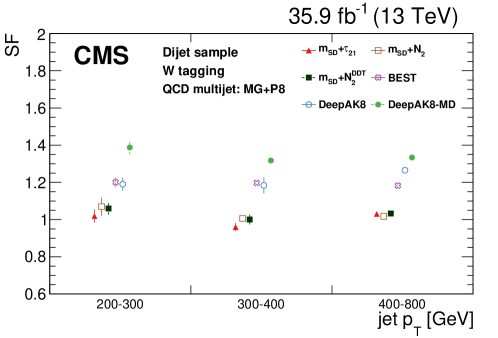
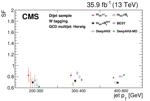
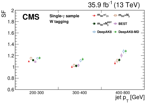
Figure 43: The ratio of the misidentification rate of  bosons in data and simulation in the dijet (upper and middle rows) and the single-$\gamma$ (lower row) samples. The QCD multijet process is simulated using for the hard process and for parton showering (upper) and for both (middle). The vertical lines correspond to the statistical uncertainty of the data and the simulated samples.

0.9 Summary

A review of the heavy-object tagging methods recently developed in CMS has been presented. The variety of tagging strategies is diverse, including algorithms based on more traditional theory-inspired high-level per-jet observables with and without multivariate techniques, as well as methods based on lower-level information from individual particles. New tagging approaches, such as the Energy Correlation Functions (ECF) tagger and the Boosted Event Shape Tagger (BEST), utilize multivariate methods (i.e., boosted decision trees and deep neural networks) on physically motivated high-level observables and attain enhanced performance. Two novel tagging algorithms, ImageTop and DeepAK8, are developed based on candidate-level information, allowing the exploitation of more information, where lower-level information is processed using advanced machine-learning methods. Moreover, the BEST and DeepAK8 algorithms are developed to provide multi-class tagging capabilities. Finally, dedicated versions of the algorithms that are only weakly correlated with the jet mass are developed. Such tools are particularly important for analyses that rely on the jet mass sidebands to estimate the background contribution under the heavy resonance mass. The mass-decorrelated algorithms ($m_{\mathrm{SD}}+N_{2}^{\mathrm{DDT}}$, ImageTop-MD, and DeepAK8-MD) typically show weaker discriminating power than their counterparts. However, they can yield better sensitivity in some physics analyses because of smaller uncertainties in background estimations.

The performances of the various tagging algorithms are directly compared using simulation in a jet range from 200 to 2000. Overall, the application of machine-learning techniques for jet tagging shows strong improvement compared to cutoff-based methods. The approaches based on low-level information yield the best performance, with as much as an order of magnitude gain in background rejection for the same signal efficiency. Another important aspect essential for the application of the new techniques in physics analysis is the systematic uncertainties associated to each algorithm. Those based on low-level features and advanced machine-learning techniques are typically prone to larger systematic uncertainties. However, these uncertainties are usually small enough to preserve the significant improvements observed. The techniques have also been validated in collision data, with scale factors extracted, including systematic uncertainties. The performances of these tagging algorithms are in good agreement between data and simulation.

.10 The CMS Collaboration

Yerevan Physics Institute, Yerevan, Armenia
A.M. Sirunyan${}^{\textrm{\textdagger}}$, A. Tumasyan Institut für Hochenergiephysik, Wien, Austria
W. Adam, F. Ambrogi, T. Bergauer, M. Dragicevic, J. Erö, A. Escalante Del Valle, M. Flechl, R. Frühwirth1, M. Jeitler1, N. Krammer, I. Krätschmer, D. Liko, T. Madlener, I. Mikulec, N. Rad, J. Schieck1, R. Schöfbeck, M. Spanring, W. Waltenberger, C.-E. Wulz1, M. Zarucki Institute for Nuclear Problems, Minsk, Belarus
V. Drugakov, V. Mossolov, J. Suarez Gonzalez Universiteit Antwerpen, Antwerpen, Belgium
M.R. Darwish, E.A. De Wolf, D. Di Croce, X. Janssen, A. Lelek, M. Pieters, H. Rejeb Sfar, H. Van Haevermaet, P. Van Mechelen, S. Van Putte, N. Van Remortel Vrije Universiteit Brussel, Brussel, Belgium
F. Blekman, E.S. Bols, S.S. Chhibra, J. D’Hondt, J. De Clercq, D. Lontkovskyi, S. Lowette, I. Marchesini, S. Moortgat, Q. Python, K. Skovpen, S. Tavernier, W. Van Doninck, P. Van Mulders Université Libre de Bruxelles, Bruxelles, Belgium
D. Beghin, B. Bilin, B. Clerbaux, G. De Lentdecker, H. Delannoy, B. Dorney, L. Favart, A. Grebenyuk, A.K. Kalsi, L. Moureaux, A. Popov, N. Postiau, E. Starling, L. Thomas, C. Vander Velde, P. Vanlaer, D. Vannerom Ghent University, Ghent, Belgium
T. Cornelis, D. Dobur, I. Khvastunov2, M. Niedziela, C. Roskas, M. Tytgat, W. Verbeke, B. Vermassen, M. Vit Université Catholique de Louvain, Louvain-la-Neuve, Belgium
O. Bondu, G. Bruno, C. Caputo, P. David, C. Delaere, M. Delcourt, A. Giammanco, V. Lemaitre, J. Prisciandaro, A. Saggio, M. Vidal Marono, P. Vischia, J. Zobec Centro Brasileiro de Pesquisas Fisicas, Rio de Janeiro, Brazil
F.L. Alves, G.A. Alves, G. Correia Silva, C. Hensel, A. Moraes, P. Rebello Teles Universidade do Estado do Rio de Janeiro, Rio de Janeiro, Brazil
E. Belchior Batista Das Chagas, W. Carvalho, J. Chinellato3, E. Coelho, E.M. Da Costa, G.G. Da Silveira4, D. De Jesus Damiao, C. De Oliveira Martins, S. Fonseca De Souza, L.M. Huertas Guativa, H. Malbouisson, J. Martins5, D. Matos Figueiredo, M. Medina Jaime6, M. Melo De Almeida, C. Mora Herrera, L. Mundim, H. Nogima, W.L. Prado Da Silva, L.J. Sanchez Rosas, A. Santoro, A. Sznajder, M. Thiel, E.J. Tonelli Manganote3, F. Torres Da Silva De Araujo, A. Vilela Pereira Universidade Estadual Paulista ^a, Universidade Federal do ABC ^b, São Paulo, Brazil
C.A. Bernardes^a, L. Calligaris^a, T.R. Fernandez Perez Tomei^a, E.M. Gregores^b, D.S. Lemos, P.G. Mercadante^b, S.F. Novaes^a, SandraS. Padula^a Institute for Nuclear Research and Nuclear Energy, Bulgarian Academy of Sciences, Sofia, Bulgaria
A. Aleksandrov, G. Antchev, R. Hadjiiska, P. Iaydjiev, M. Misheva, M. Rodozov, M. Shopova, G. Sultanov University of Sofia, Sofia, Bulgaria
M. Bonchev, A. Dimitrov, T. Ivanov, L. Litov, B. Pavlov, P. Petkov, A. Petrov Beihang University, Beijing, China
W. Fang7, X. Gao7, L. Yuan Department of Physics, Tsinghua University, Beijing, China
M. Ahmad, Z. Hu, Y. Wang Institute of High Energy Physics, Beijing, China
G.M. Chen, H.S. Chen, M. Chen, C.H. Jiang, D. Leggat, H. Liao, Z. Liu, A. Spiezia, J. Tao, E. Yazgan, H. Zhang, S. Zhang8, J. Zhao State Key Laboratory of Nuclear Physics and Technology, Peking University, Beijing, China
A. Agapitos, Y. Ban, G. Chen, A. Levin, J. Li, L. Li, Q. Li, Y. Mao, S.J. Qian, D. Wang, Q. Wang Zhejiang University, Hangzhou, China
M. Xiao Universidad de Los Andes, Bogota, Colombia
C. Avila, A. Cabrera, C. Florez, C.F. González Hernández, M.A. Segura Delgado Universidad de Antioquia, Medellin, Colombia
J. Mejia Guisao, J.D. Ruiz Alvarez, C.A. Salazar González, N. Vanegas Arbelaez University of Split, Faculty of Electrical Engineering, Mechanical Engineering and Naval Architecture, Split, Croatia
D. Giljanović, N. Godinovic, D. Lelas, I. Puljak, T. Sculac University of Split, Faculty of Science, Split, Croatia
Z. Antunovic, M. Kovac Institute Rudjer Boskovic, Zagreb, Croatia
V. Brigljevic, D. Ferencek, K. Kadija, B. Mesic, M. Roguljic, A. Starodumov9, T. Susa University of Cyprus, Nicosia, Cyprus
M.W. Ather, A. Attikis, E. Erodotou, A. Ioannou, M. Kolosova, S. Konstantinou, G. Mavromanolakis, J. Mousa, C. Nicolaou, F. Ptochos, P.A. Razis, H. Rykaczewski, D. Tsiakkouri Charles University, Prague, Czech Republic
M. Finger10, M. Finger Jr.10, A. Kveton, J. Tomsa Escuela Politecnica Nacional, Quito, Ecuador
E. Ayala Universidad San Francisco de Quito, Quito, Ecuador
E. Carrera Jarrin Academy of Scientific Research and Technology of the Arab Republic of Egypt, Egyptian Network of High Energy Physics, Cairo, Egypt
H. Abdalla11, S. Khalil12 National Institute of Chemical Physics and Biophysics, Tallinn, Estonia
S. Bhowmik, A. Carvalho Antunes De Oliveira, R.K. Dewanjee, K. Ehataht, M. Kadastik, M. Raidal, C. Veelken Department of Physics, University of Helsinki, Helsinki, Finland
P. Eerola, L. Forthomme, H. Kirschenmann, K. Osterberg, M. Voutilainen Helsinki Institute of Physics, Helsinki, Finland
F. Garcia, J. Havukainen, J.K. Heikkilä, V. Karimäki, M.S. Kim, R. Kinnunen, T. Lampén, K. Lassila-Perini, S. Laurila, S. Lehti, T. Lindén, P. Luukka, T. Mäenpää, H. Siikonen, E. Tuominen, J. Tuominiemi Lappeenranta University of Technology, Lappeenranta, Finland
T. Tuuva IRFU, CEA, Université Paris-Saclay, Gif-sur-Yvette, France
M. Besancon, F. Couderc, M. Dejardin, D. Denegri, B. Fabbro, J.L. Faure, F. Ferri, S. Ganjour, A. Givernaud, P. Gras, G. Hamel de Monchenault, P. Jarry, C. Leloup, B. Lenzi, E. Locci, J. Malcles, J. Rander, A. Rosowsky, M.Ö. Sahin, A. Savoy-Navarro13, M. Titov, G.B. Yu Laboratoire Leprince-Ringuet, CNRS/IN2P3, Ecole Polytechnique, Institut Polytechnique de Paris
S. Ahuja, C. Amendola, F. Beaudette, P. Busson, C. Charlot, B. Diab, G. Falmagne, R. Granier de Cassagnac, I. Kucher, A. Lobanov, C. Martin Perez, M. Nguyen, C. Ochando, P. Paganini, J. Rembser, R. Salerno, J.B. Sauvan, Y. Sirois, A. Zabi, A. Zghiche Université de Strasbourg, CNRS, IPHC UMR 7178, Strasbourg, France
J.-L. Agram14, J. Andrea, D. Bloch, G. Bourgatte, J.-M. Brom, E.C. Chabert, C. Collard, E. Conte14, J.-C. Fontaine14, D. Gelé, U. Goerlach, M. Jansová, A.-C. Le Bihan, N. Tonon, P. Van Hove Centre de Calcul de l’Institut National de Physique Nucleaire et de Physique des Particules, CNRS/IN2P3, Villeurbanne, France
S. Gadrat Université de Lyon, Université Claude Bernard Lyon 1, CNRS-IN2P3, Institut de Physique Nucléaire de Lyon, Villeurbanne, France
S. Beauceron, C. Bernet, G. Boudoul, C. Camen, A. Carle, N. Chanon, R. Chierici, D. Contardo, P. Depasse, H. El Mamouni, J. Fay, S. Gascon, M. Gouzevitch, B. Ille, Sa. Jain, F. Lagarde, I.B. Laktineh, H. Lattaud, A. Lesauvage, M. Lethuillier, L. Mirabito, S. Perries, V. Sordini, L. Torterotot, G. Touquet, M. Vander Donckt, S. Viret Georgian Technical University, Tbilisi, Georgia
T. Toriashvili15 Tbilisi State University, Tbilisi, Georgia
I. Bagaturia16 RWTH Aachen University, I. Physikalisches Institut, Aachen, Germany
C. Autermann, L. Feld, K. Klein, M. Lipinski, D. Meuser, A. Pauls, M. Preuten, M.P. Rauch, J. Schulz, M. Teroerde, B. Wittmer RWTH Aachen University, III. Physikalisches Institut A, Aachen, Germany
M. Erdmann, B. Fischer, S. Ghosh, T. Hebbeker, K. Hoepfner, H. Keller, L. Mastrolorenzo, M. Merschmeyer, A. Meyer, P. Millet, G. Mocellin, S. Mondal, S. Mukherjee, D. Noll, A. Novak, T. Pook, A. Pozdnyakov, T. Quast, M. Radziej, Y. Rath, H. Reithler, J. Roemer, A. Schmidt, S.C. Schuler, A. Sharma, S. Wiedenbeck, S. Zaleski RWTH Aachen University, III. Physikalisches Institut B, Aachen, Germany
G. Flügge, W. Haj Ahmad17, O. Hlushchenko, T. Kress, T. Müller, A. Nowack, C. Pistone, O. Pooth, D. Roy, H. Sert, A. Stahl18 Deutsches Elektronen-Synchrotron, Hamburg, Germany
M. Aldaya Martin, P. Asmuss, I. Babounikau, H. Bakhshiansohi, K. Beernaert, O. Behnke, A. Bermúdez Martínez, D. Bertsche, A.A. Bin Anuar, K. Borras19, V. Botta, A. Campbell, A. Cardini, P. Connor, S. Consuegra Rodríguez, C. Contreras-Campana, V. Danilov, A. De Wit, M.M. Defranchis, C. Diez Pardos, D. Domínguez Damiani, G. Eckerlin, D. Eckstein, T. Eichhorn, A. Elwood, E. Eren, E. Gallo20, A. Geiser, A. Grohsjean, M. Guthoff, M. Haranko, A. Harb, A. Jafari, N.Z. Jomhari, H. Jung, A. Kasem19, M. Kasemann, H. Kaveh, J. Keaveney, C. Kleinwort, J. Knolle, D. Krücker, W. Lange, T. Lenz, J. Lidrych, K. Lipka, W. Lohmann21, R. Mankel, I.-A. Melzer-Pellmann, A.B. Meyer, M. Meyer, M. Missiroli, J. Mnich, A. Mussgiller, V. Myronenko, D. Pérez Adán, S.K. Pflitsch, D. Pitzl, A. Raspereza, A. Saibel, M. Savitskyi, V. Scheurer, P. Schütze, C. Schwanenberger, R. Shevchenko, A. Singh, H. Tholen, O. Turkot, A. Vagnerini, M. Van De Klundert, R. Walsh, Y. Wen, K. Wichmann, C. Wissing, O. Zenaiev, R. Zlebcik University of Hamburg, Hamburg, Germany
R. Aggleton, S. Bein, L. Benato, A. Benecke, V. Blobel, T. Dreyer, A. Ebrahimi, F. Feindt, A. Fröhlich, C. Garbers, E. Garutti, D. Gonzalez, P. Gunnellini, J. Haller, A. Hinzmann, A. Karavdina, G. Kasieczka, R. Klanner, R. Kogler, N. Kovalchuk, S. Kurz, V. Kutzner, J. Lange, T. Lange, A. Malara, J. Multhaup, C.E.N. Niemeyer, A. Perieanu, A. Reimers, O. Rieger, C. Scharf, P. Schleper, S. Schumann, J. Schwandt, J. Sonneveld, H. Stadie, G. Steinbrück, F.M. Stober, B. Vormwald, I. Zoi Karlsruher Institut fuer Technologie, Karlsruhe, Germany
M. Akbiyik, C. Barth, M. Baselga, S. Baur, T. Berger, E. Butz, R. Caspart, T. Chwalek, W. De Boer, A. Dierlamm, K. El Morabit, N. Faltermann, M. Giffels, P. Goldenzweig, A. Gottmann, M.A. Harrendorf, F. Hartmann18, U. Husemann, S. Kudella, S. Mitra, M.U. Mozer, D. Müller, Th. Müller, M. Musich, A. Nürnberg, G. Quast, K. Rabbertz, M. Schröder, I. Shvetsov, H.J. Simonis, R. Ulrich, M. Wassmer, M. Weber, C. Wöhrmann, R. Wolf, S. Wozniewski Institute of Nuclear and Particle Physics (INPP), NCSR Demokritos, Aghia Paraskevi, Greece
G. Anagnostou, P. Asenov, G. Daskalakis, T. Geralis, A. Kyriakis, D. Loukas, G. Paspalaki National and Kapodistrian University of Athens, Athens, Greece
M. Diamantopoulou, G. Karathanasis, P. Kontaxakis, A. Manousakis-katsikakis, A. Panagiotou, I. Papavergou, N. Saoulidou, A. Stakia, K. Theofilatos, K. Vellidis, E. Vourliotis National Technical University of Athens, Athens, Greece
G. Bakas, K. Kousouris, I. Papakrivopoulos, G. Tsipolitis University of Ioánnina, Ioánnina, Greece
I. Evangelou, C. Foudas, P. Gianneios, P. Katsoulis, P. Kokkas, S. Mallios, K. Manitara, N. Manthos, I. Papadopoulos, J. Strologas, F.A. Triantis, D. Tsitsonis MTA-ELTE Lendület CMS Particle and Nuclear Physics Group, Eötvös Loránd University, Budapest, Hungary
M. Bartók22, R. Chudasama, M. Csanad, P. Major, K. Mandal, A. Mehta, M.I. Nagy, G. Pasztor, O. Surányi, G.I. Veres Wigner Research Centre for Physics, Budapest, Hungary
G. Bencze, C. Hajdu, D. Horvath23, F. Sikler, T.Á. Vámi, V. Veszpremi, G. Vesztergombi${}^{\textrm{\textdagger}}$ Institute of Nuclear Research ATOMKI, Debrecen, Hungary
N. Beni, S. Czellar, J. Karancsi22, J. Molnar, Z. Szillasi Institute of Physics, University of Debrecen, Debrecen, Hungary
P. Raics, D. Teyssier, Z.L. Trocsanyi, B. Ujvari Eszterhazy Karoly University, Karoly Robert Campus, Gyongyos, Hungary
T. Csorgo, W.J. Metzger, F. Nemes, T. Novak Indian Institute of Science (IISc), Bangalore, India
S. Choudhury, J.R. Komaragiri, P.C. Tiwari National Institute of Science Education and Research, HBNI, Bhubaneswar, India
S. Bahinipati25, C. Kar, G. Kole, P. Mal, V.K. Muraleedharan Nair Bindhu, A. Nayak26, D.K. Sahoo25, S.K. Swain Panjab University, Chandigarh, India
S. Bansal, S.B. Beri, V. Bhatnagar, S. Chauhan, N. Dhingra, R. Gupta, A. Kaur, M. Kaur, S. Kaur, P. Kumari, M. Lohan, M. Meena, K. Sandeep, S. Sharma, J.B. Singh, A.K. Virdi University of Delhi, Delhi, India
A. Bhardwaj, B.C. Choudhary, R.B. Garg, M. Gola, S. Keshri, Ashok Kumar, M. Naimuddin, P. Priyanka, K. Ranjan, Aashaq Shah, R. Sharma Saha Institute of Nuclear Physics, HBNI, Kolkata, India
R. Bhardwaj27, M. Bharti27, R. Bhattacharya, S. Bhattacharya, U. Bhawandeep27, D. Bhowmik, S. Dutta, S. Ghosh, B. Gomber28, M. Maity29, K. Mondal, S. Nandan, A. Purohit, P.K. Rout, G. Saha, S. Sarkar, T. Sarkar29, M. Sharan, B. Singh27, S. Thakur27 Indian Institute of Technology Madras, Madras, India
P.K. Behera, P. Kalbhor, A. Muhammad, P.R. Pujahari, A. Sharma, A.K. Sikdar Bhabha Atomic Research Centre, Mumbai, India
D. Dutta, V. Jha, V. Kumar, D.K. Mishra, P.K. Netrakanti, L.M. Pant, P. Shukla Tata Institute of Fundamental Research-A, Mumbai, India
T. Aziz, M.A. Bhat, S. Dugad, G.B. Mohanty, N. Sur, RavindraKumar Verma Tata Institute of Fundamental Research-B, Mumbai, India
S. Banerjee, S. Bhattacharya, S. Chatterjee, P. Das, M. Guchait, S. Karmakar, S. Kumar, G. Majumder, K. Mazumdar, N. Sahoo, S. Sawant Indian Institute of Science Education and Research (IISER), Pune, India
S. Dube, B. Kansal, A. Kapoor, K. Kothekar, S. Pandey, A. Rane, A. Rastogi, S. Sharma Institute for Research in Fundamental Sciences (IPM), Tehran, Iran
S. Chenarani30, E. Eskandari Tadavani, S.M. Etesami30, M. Khakzad, M. Mohammadi Najafabadi, M. Naseri, F. Rezaei Hosseinabadi University College Dublin, Dublin, Ireland
M. Felcini, M. Grunewald INFN Sezione di Bari ^a, Università di Bari ^b, Politecnico di Bari ^c, Bari, Italy
M. Abbrescia^a,b, R. Aly^a,b,31, C. Calabria^a,b, A. Colaleo^a, D. Creanza^a,c, L. Cristella^a,b, N. De Filippis^a,c, M. De Palma^a,b, A. Di Florio^a,b, W. Elmetenawee^a,b, L. Fiore^a, A. Gelmi^a,b, G. Iaselli^a,c, M. Ince^a,b, S. Lezki^a,b, G. Maggi^a,c, M. Maggi^a, J.A. Merlin, G. Miniello^a,b, S. My^a,b, S. Nuzzo^a,b, A. Pompili^a,b, G. Pugliese^a,c, R. Radogna^a, A. Ranieri^a, G. Selvaggi^a,b, L. Silvestris^a, F.M. Simone^a,b, R. Venditti^a, P. Verwilligen^a INFN Sezione di Bologna ^a, Università di Bologna ^b, Bologna, Italy
G. Abbiendi^a, C. Battilana^a,b, D. Bonacorsi^a,b, L. Borgonovi^a,b, S. Braibant-Giacomelli^a,b, R. Campanini^a,b, P. Capiluppi^a,b, A. Castro^a,b, F.R. Cavallo^a, C. Ciocca^a, G. Codispoti^a,b, M. Cuffiani^a,b, G.M. Dallavalle^a, F. Fabbri^a, A. Fanfani^a,b, E. Fontanesi^a,b, P. Giacomelli^a, C. Grandi^a, L. Guiducci^a,b, F. Iemmi^a,b, S. Lo Meo^a,32, S. Marcellini^a, G. Masetti^a, F.L. Navarria^a,b, A. Perrotta^a, F. Primavera^a,b, A.M. Rossi^a,b, T. Rovelli^a,b, G.P. Siroli^a,b, N. Tosi^a INFN Sezione di Catania ^a, Università di Catania ^b, Catania, Italy
S. Albergo^a,b,33, S. Costa^a,b, A. Di Mattia^a, R. Potenza^a,b, A. Tricomi^a,b,33, C. Tuve^a,b INFN Sezione di Firenze ^a, Università di Firenze ^b, Firenze, Italy
G. Barbagli^a, A. Cassese^a, R. Ceccarelli^a,b, V. Ciulli^a,b, C. Civinini^a, R. D’Alessandro^a,b, F. Fiori^a,c, E. Focardi^a,b, G. Latino^a,b, P. Lenzi^a,b, M. Meschini^a, S. Paoletti^a, G. Sguazzoni^a, L. Viliani^a INFN Laboratori Nazionali di Frascati, Frascati, Italy
L. Benussi, S. Bianco, D. Piccolo INFN Sezione di Genova ^a, Università di Genova ^b, Genova, Italy
M. Bozzo^a,b, F. Ferro^a, R. Mulargia^a,b, E. Robutti^a, S. Tosi^a,b INFN Sezione di Milano-Bicocca ^a, Università di Milano-Bicocca ^b, Milano, Italy
A. Benaglia^a, A. Beschi^a,b, F. Brivio^a,b, V. Ciriolo^a,b,18, M.E. Dinardo^a,b, P. Dini^a, S. Gennai^a, A. Ghezzi^a,b, P. Govoni^a,b, L. Guzzi^a,b, M. Malberti^a, S. Malvezzi^a, D. Menasce^a, F. Monti^a,b, L. Moroni^a, M. Paganoni^a,b, D. Pedrini^a, S. Ragazzi^a,b, T. Tabarelli de Fatis^a,b, D. Valsecchi^a,b, D. Zuolo^a,b INFN Sezione di Napoli ^a, Università di Napoli ’Federico II’ ^b, Napoli, Italy, Università della Basilicata ^c, Potenza, Italy, Università G. Marconi ^d, Roma, Italy
S. Buontempo^a, N. Cavallo^a,c, A. De Iorio^a,b, A. Di Crescenzo^a,b, F. Fabozzi^a,c, F. Fienga^a, G. Galati^a, A.O.M. Iorio^a,b, L. Lista^a,b, S. Meola^a,d,18, P. Paolucci^a,18, B. Rossi^a, C. Sciacca^a,b, E. Voevodina^a,b INFN Sezione di Padova ^a, Università di Padova ^b, Padova, Italy, Università di Trento ^c, Trento, Italy
P. Azzi^a, N. Bacchetta^a, D. Bisello^a,b, A. Boletti^a,b, A. Bragagnolo^a,b, R. Carlin^a,b, P. Checchia^a, P. De Castro Manzano^a, T. Dorigo^a, U. Dosselli^a, F. Gasparini^a,b, U. Gasparini^a,b, A. Gozzelino^a, S.Y. Hoh^a,b, P. Lujan^a, M. Margoni^a,b, A.T. Meneguzzo^a,b, J. Pazzini^a,b, M. Presilla^b, P. Ronchese^a,b, R. Rossin^a,b, F. Simonetto^a,b, A. Tiko^a, M. Tosi^a,b, M. Zanetti^a,b, P. Zotto^a,b, G. Zumerle^a,b INFN Sezione di Pavia ^a, Università di Pavia ^b, Pavia, Italy
A. Braghieri^a, D. Fiorina^a,b, P. Montagna^a,b, S.P. Ratti^a,b, V. Re^a, M. Ressegotti^a,b, C. Riccardi^a,b, P. Salvini^a, I. Vai^a, P. Vitulo^a,b INFN Sezione di Perugia ^a, Università di Perugia ^b, Perugia, Italy
M. Biasini^a,b, G.M. Bilei^a, D. Ciangottini^a,b, L. Fanò^a,b, P. Lariccia^a,b, R. Leonardi^a,b, E. Manoni^a, G. Mantovani^a,b, V. Mariani^a,b, M. Menichelli^a, A. Rossi^a,b, A. Santocchia^a,b, D. Spiga^a INFN Sezione di Pisa ^a, Università di Pisa ^b, Scuola Normale Superiore di Pisa ^c, Pisa, Italy
K. Androsov^a, P. Azzurri^a, G. Bagliesi^a, V. Bertacchi^a,c, L. Bianchini^a, T. Boccali^a, R. Castaldi^a, M.A. Ciocci^a,b, R. Dell’Orso^a, S. Donato^a, G. Fedi^a, L. Giannini^a,c, A. Giassi^a, M.T. Grippo^a, F. Ligabue^a,c, E. Manca^a,c, G. Mandorli^a,c, A. Messineo^a,b, F. Palla^a, A. Rizzi^a,b, G. Rolandi34, S. Roy Chowdhury, A. Scribano^a, P. Spagnolo^a, R. Tenchini^a, G. Tonelli^a,b, N. Turini^a, A. Venturi^a, P.G. Verdini^a INFN Sezione di Roma ^a, Sapienza Università di Roma ^b, Rome, Italy
F. Cavallari^a, M. Cipriani^a,b, D. Del Re^a,b, E. Di Marco^a, M. Diemoz^a, E. Longo^a,b, P. Meridiani^a, G. Organtini^a,b, F. Pandolfi^a, R. Paramatti^a,b, C. Quaranta^a,b, S. Rahatlou^a,b, C. Rovelli^a, F. Santanastasio^a,b, L. Soffi^a,b INFN Sezione di Torino ^a, Università di Torino ^b, Torino, Italy, Università del Piemonte Orientale ^c, Novara, Italy
N. Amapane^a,b, R. Arcidiacono^a,c, S. Argiro^a,b, M. Arneodo^a,c, N. Bartosik^a, R. Bellan^a,b, A. Bellora, C. Biino^a, A. Cappati^a,b, N. Cartiglia^a, S. Cometti^a, M. Costa^a,b, R. Covarelli^a,b, N. Demaria^a, B. Kiani^a,b, F. Legger, C. Mariotti^a, S. Maselli^a, E. Migliore^a,b, V. Monaco^a,b, E. Monteil^a,b, M. Monteno^a, M.M. Obertino^a,b, G. Ortona^a,b, L. Pacher^a,b, N. Pastrone^a, M. Pelliccioni^a, G.L. Pinna Angioni^a,b, A. Romero^a,b, M. Ruspa^a,c, R. Salvatico^a,b, V. Sola^a, A. Solano^a,b, D. Soldi^a,b, A. Staiano^a, D. Trocino^a,b INFN Sezione di Trieste ^a, Università di Trieste ^b, Trieste, Italy
S. Belforte^a, V. Candelise^a,b, M. Casarsa^a, F. Cossutti^a, A. Da Rold^a,b, G. Della Ricca^a,b, F. Vazzoler^a,b, A. Zanetti^a Kyungpook National University, Daegu, Korea
B. Kim, D.H. Kim, G.N. Kim, J. Lee, S.W. Lee, C.S. Moon, Y.D. Oh, S.I. Pak, S. Sekmen, D.C. Son, Y.C. Yang Chonnam National University, Institute for Universe and Elementary Particles, Kwangju, Korea
H. Kim, D.H. Moon, G. Oh Hanyang University, Seoul, Korea
B. Francois, T.J. Kim, J. Park Korea University, Seoul, Korea
S. Cho, S. Choi, Y. Go, S. Ha, B. Hong, K. Lee, K.S. Lee, J. Lim, J. Park, S.K. Park, Y. Roh, J. Yoo Kyung Hee University, Department of Physics
J. Goh Sejong University, Seoul, Korea
H.S. Kim Seoul National University, Seoul, Korea
J. Almond, J.H. Bhyun, J. Choi, S. Jeon, J. Kim, J.S. Kim, H. Lee, K. Lee, S. Lee, K. Nam, M. Oh, S.B. Oh, B.C. Radburn-Smith, U.K. Yang, H.D. Yoo, I. Yoon University of Seoul, Seoul, Korea
D. Jeon, J.H. Kim, J.S.H. Lee, I.C. Park, I.J Watson Sungkyunkwan University, Suwon, Korea
Y. Choi, C. Hwang, Y. Jeong, J. Lee, Y. Lee, I. Yu Riga Technical University, Riga, Latvia
V. Veckalns35 Vilnius University, Vilnius, Lithuania
V. Dudenas, A. Juodagalvis, A. Rinkevicius, G. Tamulaitis, J. Vaitkus National Centre for Particle Physics, Universiti Malaya, Kuala Lumpur, Malaysia
Z.A. Ibrahim, F. Mohamad Idris36, W.A.T. Wan Abdullah, M.N. Yusli, Z. Zolkapli Universidad de Sonora (UNISON), Hermosillo, Mexico
J.F. Benitez, A. Castaneda Hernandez, J.A. Murillo Quijada, L. Valencia Palomo Centro de Investigacion y de Estudios Avanzados del IPN, Mexico City, Mexico
H. Castilla-Valdez, E. De La Cruz-Burelo, I. Heredia-De La Cruz37, R. Lopez-Fernandez, A. Sanchez-Hernandez Universidad Iberoamericana, Mexico City, Mexico
S. Carrillo Moreno, C. Oropeza Barrera, M. Ramirez-Garcia, F. Vazquez Valencia Benemerita Universidad Autonoma de Puebla, Puebla, Mexico
J. Eysermans, I. Pedraza, H.A. Salazar Ibarguen, C. Uribe Estrada Universidad Autónoma de San Luis Potosí, San Luis Potosí, Mexico
A. Morelos Pineda University of Montenegro, Podgorica, Montenegro
J. Mijuskovic2, N. Raicevic University of Auckland, Auckland, New Zealand
D. Krofcheck University of Canterbury, Christchurch, New Zealand
S. Bheesette, P.H. Butler National Centre for Physics, Quaid-I-Azam University, Islamabad, Pakistan
A. Ahmad, M. Ahmad, Q. Hassan, H.R. Hoorani, W.A. Khan, M.A. Shah, M. Shoaib, M. Waqas AGH University of Science and Technology Faculty of Computer Science, Electronics and Telecommunications, Krakow, Poland
V. Avati, L. Grzanka, M. Malawski National Centre for Nuclear Research, Swierk, Poland
H. Bialkowska, M. Bluj, B. Boimska, M. Górski, M. Kazana, M. Szleper, P. Zalewski Institute of Experimental Physics, Faculty of Physics, University of Warsaw, Warsaw, Poland
K. Bunkowski, A. Byszuk38, K. Doroba, A. Kalinowski, M. Konecki, J. Krolikowski, M. Olszewski, M. Walczak Laboratório de Instrumentação e Física Experimental de Partículas, Lisboa, Portugal
M. Araujo, P. Bargassa, D. Bastos, A. Di Francesco, P. Faccioli, B. Galinhas, M. Gallinaro, J. Hollar, N. Leonardo, T. Niknejad, J. Seixas, K. Shchelina, G. Strong, O. Toldaiev, J. Varela Joint Institute for Nuclear Research, Dubna, Russia
S. Afanasiev, P. Bunin, M. Gavrilenko, I. Golutvin, I. Gorbunov, A. Kamenev, V. Karjavine, A. Lanev, A. Malakhov, V. Matveev39^,40, P. Moisenz, V. Palichik, V. Perelygin, M. Savina, S. Shmatov, S. Shulha, N. Skatchkov, V. Smirnov, N. Voytishin, A. Zarubin Petersburg Nuclear Physics Institute, Gatchina (St. Petersburg), Russia
L. Chtchipounov, V. Golovtcov, Y. Ivanov, V. Kim41, E. Kuznetsova42, P. Levchenko, V. Murzin, V. Oreshkin, I. Smirnov, D. Sosnov, V. Sulimov, L. Uvarov, A. Vorobyev Institute for Nuclear Research, Moscow, Russia
Yu. Andreev, A. Dermenev, S. Gninenko, N. Golubev, A. Karneyeu, M. Kirsanov, N. Krasnikov, A. Pashenkov, D. Tlisov, A. Toropin Institute for Theoretical and Experimental Physics named by A.I. Alikhanov of NRC ‘Kurchatov Institute’, Moscow, Russia
V. Epshteyn, V. Gavrilov, N. Lychkovskaya, A. Nikitenko43, V. Popov, I. Pozdnyakov, G. Safronov, A. Spiridonov, A. Stepennov, M. Toms, E. Vlasov, A. Zhokin Moscow Institute of Physics and Technology, Moscow, Russia
T. Aushev National Research Nuclear University ’Moscow Engineering Physics Institute’ (MEPhI), Moscow, Russia
O. Bychkova, M. Chadeeva44, P. Parygin, E. Popova, V. Rusinov P.N. Lebedev Physical Institute, Moscow, Russia
V. Andreev, M. Azarkin, I. Dremin, M. Kirakosyan, A. Terkulov Skobeltsyn Institute of Nuclear Physics, Lomonosov Moscow State University, Moscow, Russia
A. Belyaev, E. Boos, M. Dubinin45, L. Dudko, A. Ershov, A. Gribushin, V. Klyukhin, O. Kodolova, I. Lokhtin, S. Obraztsov, S. Petrushanko, V. Savrin, A. Snigirev Novosibirsk State University (NSU), Novosibirsk, Russia
A. Barnyakov46, V. Blinov46, T. Dimova46, L. Kardapoltsev46, Y. Skovpen46 Institute for High Energy Physics of National Research Centre ‘Kurchatov Institute’, Protvino, Russia
I. Azhgirey, I. Bayshev, S. Bitioukov, V. Kachanov, D. Konstantinov, P. Mandrik, V. Petrov, R. Ryutin, S. Slabospitskii, A. Sobol, S. Troshin, N. Tyurin, A. Uzunian, A. Volkov National Research Tomsk Polytechnic University, Tomsk, Russia
A. Babaev, A. Iuzhakov, V. Okhotnikov Tomsk State University, Tomsk, Russia
V. Borchsh, V. Ivanchenko, E. Tcherniaev University of Belgrade: Faculty of Physics and VINCA Institute of Nuclear Sciences
P. Adzic47, P. Cirkovic, M. Dordevic, P. Milenovic, J. Milosevic, M. Stojanovic Centro de Investigaciones Energéticas Medioambientales y Tecnológicas (CIEMAT), Madrid, Spain
M. Aguilar-Benitez, J. Alcaraz Maestre, A. Álvarez Fernández, I. Bachiller, M. Barrio Luna, CristinaF. Bedoya, J.A. Brochero Cifuentes, C.A. Carrillo Montoya, M. Cepeda, M. Cerrada, N. Colino, B. De La Cruz, A. Delgado Peris, J.P. Fernández Ramos, J. Flix, M.C. Fouz, O. Gonzalez Lopez, S. Goy Lopez, J.M. Hernandez, M.I. Josa, D. Moran, Á. Navarro Tobar, A. Pérez-Calero Yzquierdo, J. Puerta Pelayo, I. Redondo, L. Romero, S. Sánchez Navas, M.S. Soares, A. Triossi, C. Willmott Universidad Autónoma de Madrid, Madrid, Spain
C. Albajar, J.F. de Trocóniz, R. Reyes-Almanza Universidad de Oviedo, Instituto Universitario de Ciencias y Tecnologías Espaciales de Asturias (ICTEA), Oviedo, Spain
B. Alvarez Gonzalez, J. Cuevas, C. Erice, J. Fernandez Menendez, S. Folgueras, I. Gonzalez Caballero, J.R. González Fernández, E. Palencia Cortezon, V. Rodríguez Bouza, S. Sanchez Cruz Instituto de Física de Cantabria (IFCA), CSIC-Universidad de Cantabria, Santander, Spain
I.J. Cabrillo, A. Calderon, B. Chazin Quero, J. Duarte Campderros, M. Fernandez, P.J. Fernández Manteca, A. García Alonso, G. Gomez, C. Martinez Rivero, P. Martinez Ruiz del Arbol, F. Matorras, J. Piedra Gomez, C. Prieels, T. Rodrigo, A. Ruiz-Jimeno, L. Russo48, L. Scodellaro, I. Vila, J.M. Vizan Garcia University of Colombo, Colombo, Sri Lanka
D.U.J. Sonnadara University of Ruhuna, Department of Physics, Matara, Sri Lanka
W.G.D. Dharmaratna, N. Wickramage CERN, European Organization for Nuclear Research, Geneva, Switzerland
D. Abbaneo, B. Akgun, E. Auffray, G. Auzinger, J. Baechler, P. Baillon, A.H. Ball, D. Barney, J. Bendavid, M. Bianco, A. Bocci, P. Bortignon, E. Bossini, E. Brondolin, T. Camporesi, A. Caratelli, G. Cerminara, E. Chapon, G. Cucciati, D. d’Enterria, A. Dabrowski, N. Daci, V. Daponte, A. David, O. Davignon, A. De Roeck, M. Deile, M. Dobson, M. Dünser, N. Dupont, A. Elliott-Peisert, N. Emriskova, F. Fallavollita49, D. Fasanella, S. Fiorendi, G. Franzoni, J. Fulcher, W. Funk, S. Giani, D. Gigi, K. Gill, F. Glege, L. Gouskos, M. Gruchala, M. Guilbaud, D. Gulhan, J. Hegeman, C. Heidegger, Y. Iiyama, V. Innocente, T. James, P. Janot, O. Karacheban21, J. Kaspar, J. Kieseler, M. Krammer1, N. Kratochwil, C. Lange, P. Lecoq, C. Lourenço, L. Malgeri, M. Mannelli, A. Massironi, F. Meijers, S. Mersi, E. Meschi, F. Moortgat, M. Mulders, J. Ngadiuba, J. Niedziela, S. Nourbakhsh, S. Orfanelli, L. Orsini, F. Pantaleo18, L. Pape, E. Perez, M. Peruzzi, A. Petrilli, G. Petrucciani, A. Pfeiffer, M. Pierini, F.M. Pitters, D. Rabady, A. Racz, M. Rieger, M. Rovere, H. Sakulin, J. Salfeld-Nebgen, C. Schäfer, C. Schwick, M. Selvaggi, A. Sharma, P. Silva, W. Snoeys, P. Sphicas50, J. Steggemann, S. Summers, V.R. Tavolaro, D. Treille, A. Tsirou, G.P. Van Onsem, A. Vartak, M. Verzetti, W.D. Zeuner Paul Scherrer Institut, Villigen, Switzerland
L. Caminada51, K. Deiters, W. Erdmann, R. Horisberger, Q. Ingram, H.C. Kaestli, D. Kotlinski, U. Langenegger, T. Rohe, S.A. Wiederkehr ETH Zurich - Institute for Particle Physics and Astrophysics (IPA), Zurich, Switzerland
M. Backhaus, P. Berger, N. Chernyavskaya, G. Dissertori, M. Dittmar, M. Donegà, C. Dorfer, T.A. Gómez Espinosa, C. Grab, D. Hits, W. Lustermann, R.A. Manzoni, M.T. Meinhard, F. Micheli, P. Musella, F. Nessi-Tedaldi, F. Pauss, G. Perrin, L. Perrozzi, S. Pigazzini, M.G. Ratti, M. Reichmann, C. Reissel, T. Reitenspiess, B. Ristic, D. Ruini, D.A. Sanz Becerra, M. Schönenberger, L. Shchutska, M.L. Vesterbacka Olsson, R. Wallny, D.H. Zhu Universität Zürich, Zurich, Switzerland
T.K. Aarrestad, C. Amsler52, C. Botta, D. Brzhechko, M.F. Canelli, A. De Cosa, R. Del Burgo, B. Kilminster, S. Leontsinis, V.M. Mikuni, I. Neutelings, G. Rauco, P. Robmann, K. Schweiger, C. Seitz, Y. Takahashi, S. Wertz, A. Zucchetta National Central University, Chung-Li, Taiwan
T.H. Doan, C.M. Kuo, W. Lin, A. Roy, S.S. Yu National Taiwan University (NTU), Taipei, Taiwan
P. Chang, Y. Chao, K.F. Chen, P.H. Chen, W.-S. Hou, Y.y. Li, R.-S. Lu, E. Paganis, A. Psallidas, A. Steen Chulalongkorn University, Faculty of Science, Department of Physics, Bangkok, Thailand
B. Asavapibhop, C. Asawatangtrakuldee, N. Srimanobhas, N. Suwonjandee Çukurova University, Physics Department, Science and Art Faculty, Adana, Turkey
A. Bat, F. Boran, A. Celik53, S. Damarseckin54, Z.S. Demiroglu, F. Dolek, C. Dozen55, I. Dumanoglu, G. Gokbulut, EmineGurpinar Guler56, Y. Guler, I. Hos57, C. Isik, E.E. Kangal58, O. Kara, A. Kayis Topaksu, U. Kiminsu, G. Onengut, K. Ozdemir59, S. Ozturk60, A.E. Simsek, U.G. Tok, S. Turkcapar, I.S. Zorbakir, C. Zorbilmez Middle East Technical University, Physics Department, Ankara, Turkey
B. Isildak61, G. Karapinar62, M. Yalvac Bogazici University, Istanbul, Turkey
I.O. Atakisi, E. Gülmez, M. Kaya63, O. Kaya64, Ö. Özçelik, S. Tekten, E.A. Yetkin65 Istanbul Technical University, Istanbul, Turkey
A. Cakir, K. Cankocak, Y. Komurcu, S. Sen66 Istanbul University, Istanbul, Turkey
S. Cerci67, B. Kaynak, S. Ozkorucuklu, D. Sunar Cerci67 Institute for Scintillation Materials of National Academy of Science of Ukraine, Kharkov, Ukraine
B. Grynyov National Scientific Center, Kharkov Institute of Physics and Technology, Kharkov, Ukraine
L. Levchuk University of Bristol, Bristol, United Kingdom
E. Bhal, S. Bologna, J.J. Brooke, D. Burns68, E. Clement, D. Cussans, H. Flacher, J. Goldstein, G.P. Heath, H.F. Heath, L. Kreczko, B. Krikler, S. Paramesvaran, B. Penning, T. Sakuma, S. Seif El Nasr-Storey, V.J. Smith, J. Taylor, A. Titterton Rutherford Appleton Laboratory, Didcot, United Kingdom
K.W. Bell, A. Belyaev69, C. Brew, R.M. Brown, D.J.A. Cockerill, J.A. Coughlan, K. Harder, S. Harper, J. Linacre, K. Manolopoulos, D.M. Newbold, E. Olaiya, D. Petyt, T. Reis, T. Schuh, C.H. Shepherd-Themistocleous, A. Thea, I.R. Tomalin, T. Williams Imperial College, London, United Kingdom
R. Bainbridge, P. Bloch, J. Borg, S. Breeze, O. Buchmuller, A. Bundock, GurpreetSingh CHAHAL70, D. Colling, P. Dauncey, G. Davies, M. Della Negra, R. Di Maria, P. Everaerts, G. Hall, G. Iles, M. Komm, L. Lyons, A.-M. Magnan, S. Malik, A. Martelli, V. Milosevic, A. Morton, J. Nash71, V. Palladino, M. Pesaresi, D.M. Raymond, A. Richards, A. Rose, E. Scott, C. Seez, A. Shtipliyski, M. Stoye, T. Strebler, A. Tapper, K. Uchida, T. Virdee18, N. Wardle, D. Winterbottom, A.G. Zecchinelli, S.C. Zenz Brunel University, Uxbridge, United Kingdom
J.E. Cole, P.R. Hobson, A. Khan, P. Kyberd, C.K. Mackay, I.D. Reid, L. Teodorescu, S. Zahid Baylor University, Waco, USA
A. Brinkerhoff, K. Call, B. Caraway, J. Dittmann, K. Hatakeyama, C. Madrid, B. McMaster, N. Pastika, C. Smith Catholic University of America, Washington, DC, USA
R. Bartek, A. Dominguez, R. Uniyal, A.M. Vargas Hernandez The University of Alabama, Tuscaloosa, USA
A. Buccilli, S.I. Cooper, C. Henderson, P. Rumerio, C. West Boston University, Boston, USA
A. Albert, D. Arcaro, Z. Demiragli, D. Gastler, C. Richardson, J. Rohlf, D. Sperka, D. Spitzbart, I. Suarez, L. Sulak, D. Zou Brown University, Providence, USA
G. Benelli, B. Burkle, X. Coubez19, D. Cutts, Y.t. Duh, M. Hadley, U. Heintz, J.M. Hogan72, K.H.M. Kwok, E. Laird, G. Landsberg, K.T. Lau, J. Lee, M. Narain, S. Sagir73, R. Syarif, E. Usai, W.Y. Wong, D. Yu, W. Zhang University of California, Davis, Davis, USA
R. Band, C. Brainerd, R. Breedon, M. Calderon De La Barca Sanchez, M. Chertok, J. Conway, R. Conway, P.T. Cox, R. Erbacher, C. Flores, G. Funk, F. Jensen, W. Ko${}^{\textrm{\textdagger}}$, O. Kukral, R. Lander, M. Mulhearn, D. Pellett, J. Pilot, M. Shi, D. Taylor, K. Tos, M. Tripathi, Z. Wang, F. Zhang University of California, Los Angeles, USA
M. Bachtis, C. Bravo, R. Cousins, A. Dasgupta, A. Florent, J. Hauser, M. Ignatenko, N. Mccoll, W.A. Nash, S. Regnard, D. Saltzberg, C. Schnaible, B. Stone, V. Valuev University of California, Riverside, Riverside, USA
K. Burt, Y. Chen, R. Clare, J.W. Gary, S.M.A. Ghiasi Shirazi, G. Hanson, G. Karapostoli, O.R. Long, M. Olmedo Negrete, M.I. Paneva, W. Si, L. Wang, S. Wimpenny, B.R. Yates, Y. Zhang University of California, San Diego, La Jolla, USA
J.G. Branson, P. Chang, S. Cittolin, S. Cooperstein, N. Deelen, M. Derdzinski, R. Gerosa, D. Gilbert, B. Hashemi, D. Klein, V. Krutelyov, J. Letts, M. Masciovecchio, S. May, S. Padhi, M. Pieri, V. Sharma, M. Tadel, F. Würthwein, A. Yagil, G. Zevi Della Porta University of California, Santa Barbara - Department of Physics, Santa Barbara, USA
N. Amin, R. Bhandari, C. Campagnari, M. Citron, V. Dutta, M. Franco Sevilla, J. Incandela, B. Marsh, H. Mei, A. Ovcharova, H. Qu, J. Richman, U. Sarica, D. Stuart, S. Wang California Institute of Technology, Pasadena, USA
D. Anderson, A. Bornheim, O. Cerri, I. Dutta, J.M. Lawhorn, N. Lu, J. Mao, H.B. Newman, T.Q. Nguyen, J. Pata, M. Spiropulu, J.R. Vlimant, S. Xie, Z. Zhang, R.Y. Zhu Carnegie Mellon University, Pittsburgh, USA
M.B. Andrews, T. Ferguson, T. Mudholkar, M. Paulini, M. Sun, I. Vorobiev, M. Weinberg University of Colorado Boulder, Boulder, USA
J.P. Cumalat, W.T. Ford, E. MacDonald, T. Mulholland, R. Patel, A. Perloff, K. Stenson, K.A. Ulmer, S.R. Wagner Cornell University, Ithaca, USA
J. Alexander, Y. Cheng, J. Chu, A. Datta, A. Frankenthal, K. Mcdermott, J.R. Patterson, D. Quach, A. Ryd, S.M. Tan, Z. Tao, J. Thom, P. Wittich, M. Zientek Fermi National Accelerator Laboratory, Batavia, USA
S. Abdullin, M. Albrow, M. Alyari, G. Apollinari, A. Apresyan, A. Apyan, S. Banerjee, L.A.T. Bauerdick, A. Beretvas, D. Berry, J. Berryhill, P.C. Bhat, K. Burkett, J.N. Butler, A. Canepa, G.B. Cerati, H.W.K. Cheung, F. Chlebana, M. Cremonesi, J. Duarte, V.D. Elvira, J. Freeman, Z. Gecse, E. Gottschalk, L. Gray, D. Green, S. Grünendahl, O. Gutsche, J. Hanlon, R.M. Harris, S. Hasegawa, R. Heller, J. Hirschauer, B. Jayatilaka, S. Jindariani, M. Johnson, U. Joshi, T. Klijnsma, B. Klima, M.J. Kortelainen, B. Kreis, S. Lammel, J. Lewis, D. Lincoln, R. Lipton, M. Liu, T. Liu, J. Lykken, K. Maeshima, J.M. Marraffino, D. Mason, P. McBride, P. Merkel, S. Mrenna, S. Nahn, V. O’Dell, V. Papadimitriou, K. Pedro, C. Pena, G. Rakness, F. Ravera, A. Reinsvold Hall, L. Ristori, B. Schneider, E. Sexton-Kennedy, N. Smith, A. Soha, W.J. Spalding, L. Spiegel, S. Stoynev, J. Strait, N. Strobbe, L. Taylor, S. Tkaczyk, N.V. Tran, L. Uplegger, E.W. Vaandering, C. Vernieri, R. Vidal, M. Wang, H.A. Weber University of Florida, Gainesville, USA
D. Acosta, P. Avery, D. Bourilkov, L. Cadamuro, V. Cherepanov, F. Errico, R.D. Field, S.V. Gleyzer, D. Guerrero, B.M. Joshi, M. Kim, J. Konigsberg, A. Korytov, K.H. Lo, K. Matchev, N. Menendez, G. Mitselmakher, D. Rosenzweig, K. Shi, J. Wang, S. Wang, X. Zuo Florida International University, Miami, USA
Y.R. Joshi Florida State University, Tallahassee, USA
T. Adams, A. Askew, S. Hagopian, V. Hagopian, K.F. Johnson, R. Khurana, T. Kolberg, G. Martinez, T. Perry, H. Prosper, C. Schiber, R. Yohay, J. Zhang Florida Institute of Technology, Melbourne, USA
M.M. Baarmand, M. Hohlmann, D. Noonan, M. Rahmani, M. Saunders, F. Yumiceva University of Illinois at Chicago (UIC), Chicago, USA
M.R. Adams, L. Apanasevich, R.R. Betts, R. Cavanaugh, X. Chen, S. Dittmer, O. Evdokimov, C.E. Gerber, D.A. Hangal, D.J. Hofman, C. Mills, T. Roy, M.B. Tonjes, N. Varelas, J. Viinikainen, H. Wang, X. Wang, Z. Wu The University of Iowa, Iowa City, USA
M. Alhusseini, B. Bilki56, K. Dilsiz74, S. Durgut, R.P. Gandrajula, M. Haytmyradov, V. Khristenko, O.K. Köseyan, J.-P. Merlo, A. Mestvirishvili75, A. Moeller, J. Nachtman, H. Ogul76, Y. Onel, F. Ozok77, A. Penzo, C. Snyder, E. Tiras, J. Wetzel Johns Hopkins University, Baltimore, USA
B. Blumenfeld, A. Cocoros, N. Eminizer, A.V. Gritsan, W.T. Hung, S. Kyriacou, P. Maksimovic, C. Mantilla, J. Roskes, M. Swartz The University of Kansas, Lawrence, USA
C. Baldenegro Barrera, P. Baringer, A. Bean, S. Boren, J. Bowen, A. Bylinkin, T. Isidori, S. Khalil, J. King, G. Krintiras, A. Kropivnitskaya, C. Lindsey, D. Majumder, W. Mcbrayer, N. Minafra, M. Murray, C. Rogan, C. Royon, S. Sanders, E. Schmitz, J.D. Tapia Takaki, Q. Wang, J. Williams, G. Wilson Kansas State University, Manhattan, USA
S. Duric, A. Ivanov, K. Kaadze, D. Kim, Y. Maravin, D.R. Mendis, T. Mitchell, A. Modak, A. Mohammadi Lawrence Livermore National Laboratory, Livermore, USA
F. Rebassoo, D. Wright University of Maryland, College Park, USA
A. Baden, O. Baron, A. Belloni, S.C. Eno, Y. Feng, N.J. Hadley, S. Jabeen, G.Y. Jeng, R.G. Kellogg, A.C. Mignerey, S. Nabili, F. Ricci-Tam, M. Seidel, Y.H. Shin, A. Skuja, S.C. Tonwar, K. Wong Massachusetts Institute of Technology, Cambridge, USA
D. Abercrombie, B. Allen, R. Bi, S. Brandt, W. Busza, I.A. Cali, M. D’Alfonso, G. Gomez Ceballos, M. Goncharov, P. Harris, D. Hsu, M. Hu, M. Klute, D. Kovalskyi, Y.-J. Lee, P.D. Luckey, B. Maier, A.C. Marini, C. Mcginn, C. Mironov, S. Narayanan, X. Niu, C. Paus, D. Rankin, C. Roland, G. Roland, Z. Shi, G.S.F. Stephans, K. Sumorok, K. Tatar, D. Velicanu, J. Wang, T.W. Wang, B. Wyslouch University of Minnesota, Minneapolis, USA
R.M. Chatterjee, A. Evans, S. Guts${}^{\textrm{\textdagger}}$, P. Hansen, J. Hiltbrand, Sh. Jain, Y. Kubota, Z. Lesko, J. Mans, M. Revering, R. Rusack, R. Saradhy, N. Schroeder, M.A. Wadud University of Mississippi, Oxford, USA
J.G. Acosta, S. Oliveros University of Nebraska-Lincoln, Lincoln, USA
K. Bloom, S. Chauhan, D.R. Claes, C. Fangmeier, L. Finco, F. Golf, R. Kamalieddin, I. Kravchenko, J.E. Siado, G.R. Snow${}^{\textrm{\textdagger}}$, B. Stieger, W. Tabb State University of New York at Buffalo, Buffalo, USA
G. Agarwal, C. Harrington, I. Iashvili, A. Kharchilava, C. McLean, D. Nguyen, A. Parker, J. Pekkanen, S. Rappoccio, B. Roozbahani Northeastern University, Boston, USA
G. Alverson, E. Barberis, C. Freer, Y. Haddad, A. Hortiangtham, G. Madigan, B. Marzocchi, D.M. Morse, T. Orimoto, L. Skinnari, A. Tishelman-Charny, T. Wamorkar, B. Wang, A. Wisecarver, D. Wood Northwestern University, Evanston, USA
S. Bhattacharya, J. Bueghly, A. Gilbert, T. Gunter, K.A. Hahn, N. Odell, M.H. Schmitt, K. Sung, M. Trovato, M. Velasco University of Notre Dame, Notre Dame, USA
R. Bucci, N. Dev, R. Goldouzian, M. Hildreth, K. Hurtado Anampa, C. Jessop, D.J. Karmgard, K. Lannon, W. Li, N. Loukas, N. Marinelli, I. Mcalister, F. Meng, Y. Musienko39, R. Ruchti, P. Siddireddy, G. Smith, S. Taroni, M. Wayne, A. Wightman, M. Wolf, A. Woodard The Ohio State University, Columbus, USA
J. Alimena, B. Bylsma, L.S. Durkin, B. Francis, C. Hill, W. Ji, A. Lefeld, T.Y. Ling, B.L. Winer Princeton University, Princeton, USA
G. Dezoort, P. Elmer, J. Hardenbrook, N. Haubrich, S. Higginbotham, A. Kalogeropoulos, S. Kwan, D. Lange, M.T. Lucchini, J. Luo, D. Marlow, K. Mei, I. Ojalvo, J. Olsen, C. Palmer, P. Piroué, D. Stickland, C. Tully University of Puerto Rico, Mayaguez, USA
S. Malik, S. Norberg Purdue University, West Lafayette, USA
A. Barker, V.E. Barnes, R. Chawla, S. Das, L. Gutay, M. Jones, A.W. Jung, A. Khatiwada, B. Mahakud, D.H. Miller, G. Negro, N. Neumeister, C.C. Peng, S. Piperov, H. Qiu, J.F. Schulte, N. Trevisani, F. Wang, R. Xiao, W. Xie Purdue University Northwest, Hammond, USA
T. Cheng, J. Dolen, N. Parashar Rice University, Houston, USA
A. Baty, U. Behrens, S. Dildick, K.M. Ecklund, S. Freed, F.J.M. Geurts, M. Kilpatrick, Arun Kumar, W. Li, B.P. Padley, R. Redjimi, J. Roberts, J. Rorie, W. Shi, A.G. Stahl Leiton, Z. Tu, A. Zhang University of Rochester, Rochester, USA
A. Bodek, P. de Barbaro, R. Demina, J.L. Dulemba, C. Fallon, T. Ferbel, M. Galanti, A. Garcia-Bellido, O. Hindrichs, A. Khukhunaishvili, E. Ranken, R. Taus Rutgers, The State University of New Jersey, Piscataway, USA
B. Chiarito, J.P. Chou, A. Gandrakota, Y. Gershtein, E. Halkiadakis, A. Hart, M. Heindl, E. Hughes, S. Kaplan, I. Laflotte, A. Lath, R. Montalvo, K. Nash, M. Osherson, H. Saka, S. Salur, S. Schnetzer, S. Somalwar, R. Stone, S. Thomas University of Tennessee, Knoxville, USA
H. Acharya, A.G. Delannoy, S. Spanier Texas A&M University, College Station, USA
O. Bouhali78, M. Dalchenko, M. De Mattia, A. Delgado, R. Eusebi, J. Gilmore, T. Huang, T. Kamon79, H. Kim, S. Luo, S. Malhotra, D. Marley, R. Mueller, D. Overton, L. Perniè, D. Rathjens, A. Safonov Texas Tech University, Lubbock, USA
N. Akchurin, J. Damgov, F. De Guio, V. Hegde, S. Kunori, K. Lamichhane, S.W. Lee, T. Mengke, S. Muthumuni, T. Peltola, S. Undleeb, I. Volobouev, Z. Wang, A. Whitbeck Vanderbilt University, Nashville, USA
S. Greene, A. Gurrola, R. Janjam, W. Johns, C. Maguire, A. Melo, H. Ni, K. Padeken, F. Romeo, P. Sheldon, S. Tuo, J. Velkovska, M. Verweij University of Virginia, Charlottesville, USA
M.W. Arenton, P. Barria, B. Cox, G. Cummings, J. Hakala, R. Hirosky, M. Joyce, A. Ledovskoy, C. Neu, B. Tannenwald, Y. Wang, E. Wolfe, F. Xia Wayne State University, Detroit, USA
R. Harr, P.E. Karchin, N. Poudyal, J. Sturdy, P. Thapa University of Wisconsin - Madison, Madison, WI, USA
T. Bose, J. Buchanan, C. Caillol, D. Carlsmith, S. Dasu, I. De Bruyn, L. Dodd, C. Galloni, H. He, M. Herndon, A. Hervé, U. Hussain, A. Lanaro, A. Loeliger, K. Long, R. Loveless, J. Madhusudanan Sreekala, A. Mallampalli, D. Pinna, T. Ruggles, A. Savin, V. Sharma, W.H. Smith, D. Teague, S. Trembath-reichert †: Deceased
1: Also at Vienna University of Technology, Vienna, Austria
2: Also at IRFU, CEA, Université Paris-Saclay, Gif-sur-Yvette, France
3: Also at Universidade Estadual de Campinas, Campinas, Brazil
4: Also at Federal University of Rio Grande do Sul, Porto Alegre, Brazil
5: Also at UFMS, Nova Andradina, Brazil
6: Also at Universidade Federal de Pelotas, Pelotas, Brazil
7: Also at Université Libre de Bruxelles, Bruxelles, Belgium
8: Also at University of Chinese Academy of Sciences, Beijing, China
9: Also at Institute for Theoretical and Experimental Physics named by A.I. Alikhanov of NRC ‘Kurchatov Institute’, Moscow, Russia
10: Also at Joint Institute for Nuclear Research, Dubna, Russia
11: Also at Cairo University, Cairo, Egypt
12: Also at Zewail City of Science and Technology, Zewail, Egypt
13: Also at Purdue University, West Lafayette, USA
14: Also at Université de Haute Alsace, Mulhouse, France
15: Also at Tbilisi State University, Tbilisi, Georgia
16: Also at Ilia State University, Tbilisi, Georgia
17: Also at Erzincan Binali Yildirim University, Erzincan, Turkey
18: Also at CERN, European Organization for Nuclear Research, Geneva, Switzerland
19: Also at RWTH Aachen University, III. Physikalisches Institut A, Aachen, Germany
20: Also at University of Hamburg, Hamburg, Germany
21: Also at Brandenburg University of Technology, Cottbus, Germany
22: Also at Institute of Physics, University of Debrecen, Debrecen, Hungary, Debrecen, Hungary
23: Also at Institute of Nuclear Research ATOMKI, Debrecen, Hungary
24: Also at MTA-ELTE Lendület CMS Particle and Nuclear Physics Group, Eötvös Loránd University, Budapest, Hungary, Budapest, Hungary
25: Also at IIT Bhubaneswar, Bhubaneswar, India, Bhubaneswar, India
26: Also at Institute of Physics, Bhubaneswar, India
27: Also at Shoolini University, Solan, India
28: Also at University of Hyderabad, Hyderabad, India
29: Also at University of Visva-Bharati, Santiniketan, India
30: Also at Isfahan University of Technology, Isfahan, Iran
31: Now at INFN Sezione di Bari ^a, Università di Bari ^b, Politecnico di Bari ^c, Bari, Italy
32: Also at Italian National Agency for New Technologies, Energy and Sustainable Economic Development, Bologna, Italy
33: Also at Centro Siciliano di Fisica Nucleare e di Struttura Della Materia, Catania, Italy
34: Also at Scuola Normale e Sezione dell’INFN, Pisa, Italy
35: Also at Riga Technical University, Riga, Latvia, Riga, Latvia
36: Also at Malaysian Nuclear Agency, MOSTI, Kajang, Malaysia
37: Also at Consejo Nacional de Ciencia y Tecnología, Mexico City, Mexico
38: Also at Warsaw University of Technology, Institute of Electronic Systems, Warsaw, Poland
39: Also at Institute for Nuclear Research, Moscow, Russia
40: Now at National Research Nuclear University ’Moscow Engineering Physics Institute’ (MEPhI), Moscow, Russia
41: Also at St. Petersburg State Polytechnical University, St. Petersburg, Russia
42: Also at University of Florida, Gainesville, USA
43: Also at Imperial College, London, United Kingdom
44: Also at P.N. Lebedev Physical Institute, Moscow, Russia
45: Also at California Institute of Technology, Pasadena, USA
46: Also at Budker Institute of Nuclear Physics, Novosibirsk, Russia
47: Also at Faculty of Physics, University of Belgrade, Belgrade, Serbia
48: Also at Università degli Studi di Siena, Siena, Italy
49: Also at INFN Sezione di Pavia ^a, Università di Pavia ^b, Pavia, Italy, Pavia, Italy
50: Also at National and Kapodistrian University of Athens, Athens, Greece
51: Also at Universität Zürich, Zurich, Switzerland
52: Also at Stefan Meyer Institute for Subatomic Physics, Vienna, Austria, Vienna, Austria
53: Also at Burdur Mehmet Akif Ersoy University, BURDUR, Turkey
54: Also at Şırnak University, Sirnak, Turkey
55: Also at Department of Physics, Tsinghua University, Beijing, China, Beijing, China
56: Also at Beykent University, Istanbul, Turkey, Istanbul, Turkey
57: Also at Istanbul Aydin University, Application and Research Center for Advanced Studies (App. & Res. Cent. for Advanced Studies), Istanbul, Turkey
58: Also at Mersin University, Mersin, Turkey
59: Also at Piri Reis University, Istanbul, Turkey
60: Also at Gaziosmanpasa University, Tokat, Turkey
61: Also at Ozyegin University, Istanbul, Turkey
62: Also at Izmir Institute of Technology, Izmir, Turkey
63: Also at Marmara University, Istanbul, Turkey
64: Also at Kafkas University, Kars, Turkey
65: Also at Istanbul Bilgi University, Istanbul, Turkey
66: Also at Hacettepe University, Ankara, Turkey
67: Also at Adiyaman University, Adiyaman, Turkey
68: Also at Vrije Universiteit Brussel, Brussel, Belgium
69: Also at School of Physics and Astronomy, University of Southampton, Southampton, United Kingdom
70: Also at IPPP Durham University, Durham, United Kingdom
71: Also at Monash University, Faculty of Science, Clayton, Australia
72: Also at Bethel University, St. Paul, Minneapolis, USA, St. Paul, USA
73: Also at Karamanoğlu Mehmetbey University, Karaman, Turkey
74: Also at Bingol University, Bingol, Turkey
75: Also at Georgian Technical University, Tbilisi, Georgia
76: Also at Sinop University, Sinop, Turkey
77: Also at Mimar Sinan University, Istanbul, Istanbul, Turkey
78: Also at Texas A&M University at Qatar, Doha, Qatar
79: Also at Kyungpook National University, Daegu, Korea, Daegu, Korea