Quality Prediction on Deep Generative Images

Abstract

In recent years, deep neural networks have been utilized in a wide variety of applications including image generation. In particular, generative adversarial networks (GANs) are able to produce highly realistic pictures as part of tasks such as image compression. As with standard compression, it is desirable to be able to automatically assess the perceptual quality of generative images to monitor and control the encode process. However, existing image quality algorithms are ineffective on GAN generated content, especially on textured regions and at high compressions. Here we propose a new “naturalness”-based image quality predictor for generative images. Our new GAN picture quality predictor is built using a multi-stage parallel boosting system based on structural similarity features and measurements of statistical similarity. To enable model development and testing, we also constructed a subjective GAN image quality database containing (distorted) GAN images and collected human opinions of them. Our experimental results indicate that our proposed GAN IQA model delivers superior quality predictions on the generative image datasets, as well as on traditional image quality datasets.

I Introduction

Deep neural networks (DNNs) have been applied to broad swathes of applications beyond traditional computer vision, including super-resolution [1], detection [2] and classification [3] problems, and even for composing music [4] and creating computer-generated art work [5]. Of particular interest are generative adversarial networks (GANs) [6], which can learn models of highly non-linear distributions in an unsupervised manner. For example, GANs have been shown to be able to compute highly realistic, naturalistic images by capturing both global semantic information and local textural descriptions of real-world image data [7, 8]. In this direction, GANs have recently been utilized for image/video compression [9]. One approach is to create a hybrid codec combining a GAN with a legacy codec such as H.264 or HEVC (High Efficiency Video Coding) [10, 11]. At the decoder side, uncompressed regions can be synthesized using a pre-trained GAN that processes transmitted texture parameters. Another approach is to encode the entire full-resolution image using a GAN, which could be particularly effective at very low bitrates [12]. While research on GAN-based compression is in its infancy, expectations are high, because generative images are often visually pleasing and GAN-based compression has the potential to supply competitive compression efficiency.

(a) Original Image

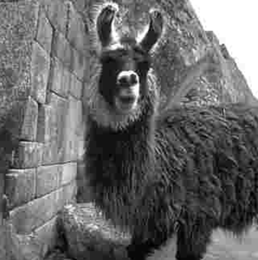
(b) JPEG (PSNR: 25.3dB)

(c) CNN (PSNR: 26.3dB)

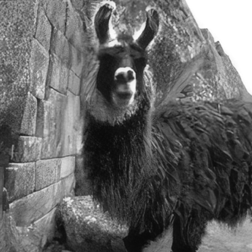
(d) GAN (PSNR: 23.5dB)

Figure 1: Examples of DNN based generative images: (a) original image, (b) JPEG-coded image, (c) CNN-generated image, and (d) GAN image.

An important aspect of the development of generative image compression systems is the ability to objectively measure the perceptual quality of the reconstructed (decoded) images. Since the characteristics of generative images are quite different from those of natural images, existing image quality assessment (IQA) models are inadequate for measuring the quality of generative images. The principle reason for this is that images generated by a GAN may appear quite realistic and similar to an original, yet may match it poorly based on pixel comparisons. For example, an original image and three versions of it created using different schemes are shown in Fig. 1. Here, the JPEG-coded image (Fig. 1(b)) is afflicted by clearly visible blocking artifacts, while an image that was generated using a CNN (convolutional neural network) is blurred. By comparison, the GAN-generated image appears looks as natural and realistic as the original. However, the peak signal to noise ratio (PSNR) values indicate otherwise, indicating the inconsistency of pixel comparisons when evaluating GAN images.
Towards addressing this problem, we propose a novel full-reference quality assessment model for analyzing generative images. The contributions that we make are summarized as follows:

• Our proposed GAN IQA model utilizes measurements of both statistical similarity and structural similarity between a reference image and a possibly distorted version of it. Statistical similarity is expressed by multiple quality-related histogram distances computed between the reference and test images. These measures effectively capture the textural characteristic of GAN-generated images and their perceptual similarity to the images they were generated from. The later is realized by deriving quality-sensitive spatial and spectral structure features based on the singular value decomposition (SVD). The final predicted scores are generated using a multi-stage parallel boosting system based on support vector regression (SVR).

• We built a generative image database by using a GAN designed for artifact removal. The new database comprises reference images that span a wide range of natural scene characteristics. These images were systematically distorted using JPEG compression as well as by generation by both CNNs and GANs (i.e. with an adversarial loss term). Unlike most other datasets, our database is divided into four data subsets, one containing full-frame images, and three subsets containing patches having different structural peculiarities, to enable a deeper analysis of both the global and local attributes of generative images. We also conducted a human subjective test utilizing the pairwise comparison method, yielding a substantial set of MOS (mean opinion scores).

• We conducted a comprehensive set of algorithm comparison experiments. First, we analyzed the per-feature group efficacy of the statistical and structural features. In addition, we also compared our proposed model with thirteen existing full-reference picture quality models as well as two recent deep learning system-based IQA modes. Furthermore, we tested our model on the three traditional image quality databases: LIVE, TID2013 and CSIQ, where it is shown to have the capability to predict the perceptual quality of natural distorted images, as well as generative images. Lastly, we performed a set of cross-database tests to evaluate the database independence of our model.

The rest of the paper is organized as follows. We review related work on image quality assessment and GAN-based image/video compression in Section II. The construction of our generative image database is detailed in Section III, while the proposed generative image quality model is introduced in Section IV. Experimental results and their discussions are provided in Section V. Finally, concluding remarks are given in Section VI.

II Related Work

II-A Image Quality Assessment

IQA models are usually classified as full-reference (FR), reduced-reference (RR), or no-reference (NR), depending on the availability of a reference image. A variety of picture quality engines based on natural scene statistic (NSS) features have been proposed, which do not rely on any strong distortion hypotheses, such as specific impairment types. Instead, these models exploit certain statistical regularities that exist in natural scene data, which are disturbed or lost in the presence of image distortions. Moorthy et al. and Saad et al. proposed “quality-aware” NSS features in the wavelet domain [14] and in the discrete cosine transform domain [15], respectively, while Mittal et al. developed similar features in the spatial domain [16]. These and many other IQA models use machine learning to capture the highly non-linear relationship between handcrafted NSS features and human judgments of picture quality. Other examples include Li et al. [17] who deployed a general regression neural network to learn a mapping between several features and picture quality, including phase congruency, entropy and the gradient. Other examples include the multi-metric fusion (MMF) model [18], the 3-D multi scorers fusion model [19], and a sparse representation of NSS features [20].
More recently, IQA models developed using deep learning have been emerging. Li et al. [21] fed the NSS-related features into a stacked autoencoder to reinforce quality prediction accuracy while Ghadiyaram et al. [22] deployed an a large variety of NSS features to train a deep belief network (DBN) to predict subjective picture quality. Rather than designing handcrafted features, the authors of [23] automatically learned features when training a CNN to generate local quality maps and conduct NR IQA. In [24], Kim et al. proposed a CNN-based FR IQA model that learns the underlying data distribution and uses it to optimize a set of visual weights, without using any prior knowledge of the HVS. A survey of deep learning methods for IQA is given in [25].

II-B GAN Based Image/Video Compression

Methods of using DNNs for data compression have recently become an active area of research. Over the last few years, the most popular DNN architecture for image compression has been various forms of the auto-encoder [26, 27, 28, 29]. An autoencoder based image compressor generates latent vectors as bit-streams, then encodes them using entropy coding. They usually use a mean-squared error (MSE) or perceptual loss functions like MS-SSIM  [30, 31] to reduce perceived distortions between the original and the decompressed images. Another popular trend is to take the adversarial loss of GAN into account, because it is capable of maintaining both global structure and local texture even of very low bitrates. However, the aforementioned loss terms may fail when reconstructing semantic information, because they favor the preservation of pixel-wise fidelity. Rippel et al. [32] used an adversarial loss to train a deep compression system, while Santurkar et al. trained a GAN framework to decode thumbnail images [33]. Eirikur et al. [9] proposed a GAN-based compression system targeting bitrates below 0.1 bit per pixel. Their system realistically synthesizes image objects and textures like streets and trees. They also increase the coding gain using a semantic label map.
GANs can be also used to pre-/post-process compressed images. For example, Galteri et al. presented a feed-forward model trained by a GAN to remove compression artifacts [34]. The authors in [7] train a GAN to perform image super-resolution (SR) with photo-realism for upscaling factors as large as 4x. While GAN-based video coding is still in early stages of development, a number of researchers are trying to replace the traditional hybrid codec framework (e.g., H.264 or HEVC) with end-to-end deep learning frameworks. In these efforts, the focus of the GAN is primary on prediction and reconstruction [35, 36], quantization [37] and pixel motion estimation [38, 39]. Recently, Kim et al. proposed a soft edge-guided conditional GAN framework targeting streaming videos at very low bitrates [12].
The notation of “picture quality” takes on a somewhat different flavor in the context of assessing generative images, which is why a new family of picture quality models is needed. This is particularly true in the context of FR IQA, as exemplified by the SSIM [30, 31] and VIF [40] models. FR models that make pixel-wise comparisons - even over neighborhoods or in a transformed space - are ultimately best characterized as perceptual fidelity measurements. NR IQA models such as BRISQUE [41] and NIQE [16] supply a different way, where only the appearance of quality of an image is assessed, but these algorithms do not make use of valuable reference information. Our approach shares elements of both; a reference picture is deployed in the evaluation, but the GAN IQA evaluator also assesses the test picture in regards to its intrinsic natural quality. This is important since, when an image is compressed, textured areas may be replaced by generative (synthesized) content instead of being encoded directly [9]. For example, the furry parts of the llama generated by the GAN in Fig. 1(d) appear sharp and natural more so than in Figs. 1(b) and 1(c), giving a more visually pleasing appearance although the content is not a good pixel-wise match to the original furry parts. Maintaining the ‘naturalness’ of generative images or subimages, while still contributing a good representation of the original can be important, since it may afford the possibility of much higher compressions while ensuring that the generative images or subimages appear both highly similar to the original as well as naturalistic.

III Generative Image Database

The new database contains four subsets; one of full-frames images and three of image patches. The patch subsets were designed to exhibit different degrees of structural complexity. Specifically, we grouped them as: 1) random structured patches, 2) regular structured (pattern) patches and 3) high-level structured (face) patches. We conducted a subjective human study on these images and patches to supply ground truth in our effort to learn a mapping between generative images and human opinions of them.

III-A Database Generation

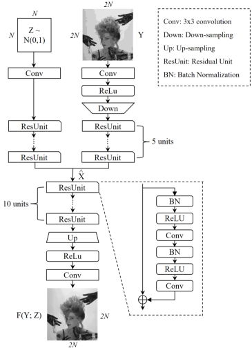
Figure 2: The GAN architecture used to build the generative image database.

(a)

(b)

(c)

(d)

(e)

(f)

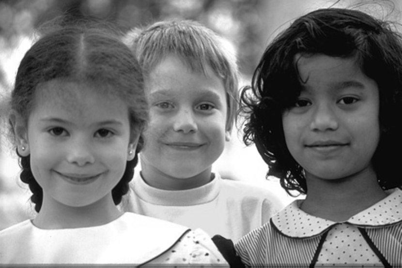
(g)

(h)

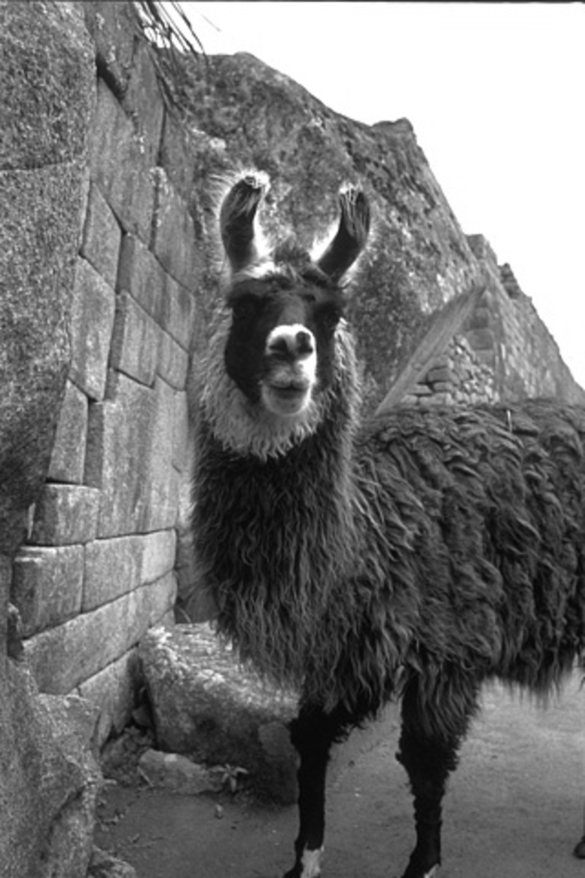
(i)

(j)

(k)

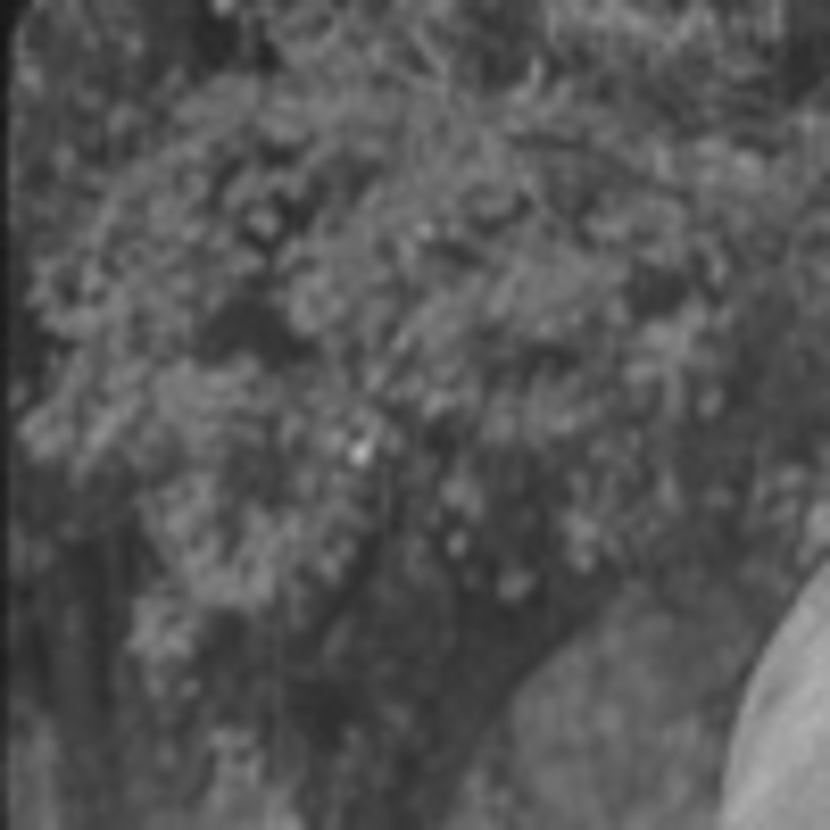
(l)

(m)

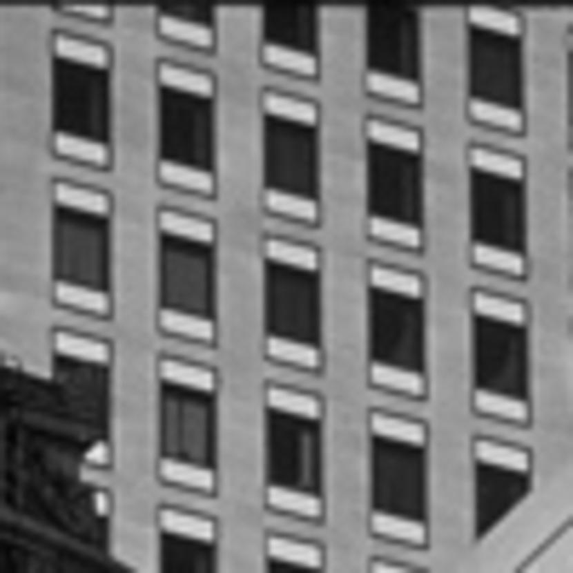
(n)

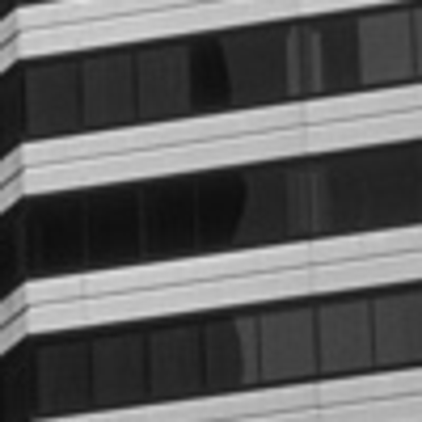
(o)

(p)

(q)

(r)

Figure 3: The reference images of the generative image database: (a)-(i) subset of full-resolution images, (j)-(l) subset of random structured patches, (m)-(o) subset of regular structured patches, (p)-(r) subset of high-level structured patches. The images and patches are not shown at relative scale.

In [42], the authors proposed an one-to-many GAN to remove artifacts from JPEG-coded images. We adopted their network with some modifications to build our generative image database. Fig. 2 shows the architecture of [42], where the image $Y$ is a JPEG compressed version of ground truth image $X$, and where random unit normal white Gaussian image $Z\sim N(0,1)$ are used as the inputs to the CNNs. The outputs of the two branches are then concatenated into a matrix $\hat{X}$, and fed into the following network, which is trained to choose the highest quality result, in the sense of both fidelity and naturalness. The objective function that is used to train the network has three terms:

where $L_{percept}$ is the perceptual loss incurred when estimating the similarity in structure. $L_{similar}$ is an adversarial loss term, while $L_{jpg}$ measures color distortion. We depart from [42] by removing $L_{jpg}$ from (1), hence our cost function becomes:

where $L_{percept}=\frac{1}{H_{\phi}}|\phi(\hat{X})-\phi(X)|^{2}$, and $\phi$ are the activations of the last convolutional layer of VGG-16 [43] while $H_{\phi}$ is the size of $\phi$. $L_{similar}$ is defined as $-log(D(\hat{X}))$, where $D$ is an additional network that distinguishes whether an image is from the network or is like the original image. To train the network $D$, a binary entropy loss is used as optimization cost: $L_{D}(X,\hat{X})=-(log(D(X)+log(1-D(\hat{X}))$. Unlike [42], we employed the Microsoft COCO dataset [44] to train the network, and the truncated normal initializer was used to initialize the weights.

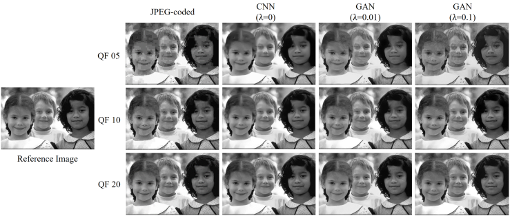
Figure 4: Examples of generated test images (first column: JPEG-coded images, second column: CNN images, third column: GAN images with $\lambda$=0.01, fourth column: GAN images with $\lambda$=0.1)

To create the generative image database, we chose 9 reference images of resolutions 480x320 or 320x480 from the BSDS500 dataset [45], which contains a wide variety of natural scene characteristics. We also created three sets of patch images of resolution 100x100 cropped from the full-resolution reference images: 1) a randomly structured patch set including three textured patches of a lawn, a furry llama and a piece of cloth, 2) a regular, structured patch set containing three repetitive patterned patches from the reference image of buildings, and 3) a high-level structured patch set containing human faces. Overall, the database contains 18 reference images, all of which are shown in Fig. 3.
Each reference image was subjected to (matlab) JPEG compression using three different quality factors: QF5 (low quality), QF10 (moderate quality) and QF20 (high quality). Next, for each of the three compressed images, we used the network in Fig. 2 to generate two generative images using weighting factor $\lambda=0.01$ and $\lambda=0.1$, respectively, in Eq. (2). We have observed that as the value of $\lambda$ is increased, the resulting generative image becomes shaper and naturalistic, but becomes less natural if $\lambda$ becomes too large. We also generated an image using the same network, but replacing $L_{percept}$ with the MSE (mean-squared error) and setting $\lambda=0$, which we designate as the CNN-generated image. In this case, since there is no adversarial loss term and the maintenance of pixel-wise fidelity is the only objective cost, the resulting generative images tend to be blurred. To sum up, there are 12 test images associated with each of the 12 reference images: 3 JPEG quality factors $\times$ {1 JPEG-coded images + 1 CNN image + 2 GAN generative images}. An example of a reference image and the 12 images generated from it are shown in Fig. 4.

III-B Subjective Study

We conducted a human study to obtain MOS (mean opinion scores) on the generative image database. In general, there are two kinds of subjective evaluation methods that are widely used in IQA studies. While the ACR (absolute category rating) recommended by the international telecommunication union (ITU) [46] for image/video quality assessment is most widely used, we chose to instead use the pairwise comparison (PC) method. We decided this because GAN-generated distortions are a relatively new phenomenon, and we wanted to be sure that subtleties of texture and detailed distortion could be better detected. The obtained human judgments were converted into numerical scores to provide subjective ground truth. During each session, when a reference image was displayed, a test image A and a test image B were displayed below it in random left-right order together per each viewing. Three questions were then asked:

• (N) Which test image looks more natural? (For this question, it is not necessary to compare each test image with the reference image.)

• (S) Which test image better preserves structural fidelity with respect to the reference image?

• (C) Which test image better preserves the concept of the contents with respect to the reference image?

As a result, three different MOS values were acquired on each pair of test images. As mentioned in Section II, GAN generative images may appear very natural while numerically differing from an original image in a pixel-wise comparison, especially in highly textured regions. Conversely, dominant structures such as the shapes and boundaries of objects might be well maintained in the GAN images. The final question was directed towards the preservation of recognizability in the image.
The outcome of a series of pairwise comparisons by a single human is an ordered list of images. However, applying the PC method using a round-robin design is very time-consuming. For instance, if there are $N$ samples, then the total number of possible pairwise comparisons is $C_{2}^{N}$. To solve the complexity issue, we instead adopt the more efficient Swiss-rule design as used in [47]. Once an assessor finishes a session, a preference matrix is created. By aggregating the preference matrices of all the assessors, a group preference matrix is obtained, which includes the count of preferred images over all the possible pairs. If $P(i,j)$ is the $(i,j)^{th}$ element of the group preference matrix, then $P(i,j)$ is the total number of times that the assessor preferred image $i$ to image $j$. The averaged count data is then used as a form of MOS. There are also two well-known ways to convert pairwise comparison data into psychophysical scores: the Bradley-Terry (BT) [48] model, and the Thurstone-Mosteller (TM) model [49]. We found that the averaged count data and the converted scores to be highly correlated with each other (Pearson correlation coefficient value = 0.984), hence, we opted for simplicity and used the counting data.
The experiment was conducted using an LG 65 inch UHDTV, and a graphical user interface (GUI) implemented in Matlab. In each presentation, a reference image was shown at the top of the screen and a randomly selected pair of test images was shown below. Each assessor was given three choices: ‘the left one is better’, ‘the right one is better’, or ‘no difference’. Further, the assessors were asked to answer the abovementioned three questions. We divided each overall session into two sub-sessions, each of duration ranging from 20 to 30 min, to meet the recommendation of ITU [46] that the duration of each session should not exceed 30 min to avoid subject fatigue. 24 assessors participated in total, and the overall session duration and each decision made by every assessor was recorded. There were nineteen males and five females. Eight of them were in their 20s and the remining 16 were in their 30s. We also filtered abnormal results according to [46]. Finally, we collected 20 opinion scores on each test image.

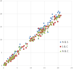
(a) Full-resolution images.

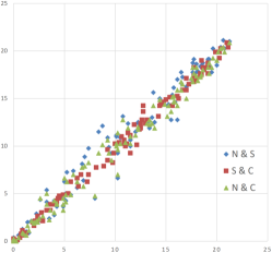
(b) Patch images.

Figure 5: Scatter plots among MOS of naturalness, structural fidelity, and concept preservation, where each dot represents one test image.

TABLE I: Summary of the generative database and the subjective test.

		Subset of Full-Resolution Images	Subsets of Image Patches
			Random Structure	Regular Structure	High-level Structured
Generative Database	# Reference images selected from BSDS500 (Resolution)	9 (480x320 or 320x480)	3 (100x100)	3 (100x100)	3 (100x100)
	Test image design	Per each reference image:
		[1] Three JPEG-coded images with QF5(low quality), QF10(moderate quality), and QF20(high quality)
		[2] For each JPEG-coded image, two GAN images were generated using $\lambda=0.1$ and $\lambda=0.01$ in (2).
		[3] For each JPEG-coded image, one CNN image was obtained using $\lambda=0$ and $L_{percept}$ = MSE
	# of test images	Total: 18 ref. images x 3 QF x (1 JPEG-coded + 1 CNN + 2 GAN img) = 216 images
Subjective Test	Study Methodology	Pairwise Comparisons
	# of participants	20
	Three independent mean subject scores	[1] Naturalness (used in the experiments)
		[2] Structural fidelity
		[3] Concept preservation

Figs. 5(a) and 5(b) show the scatter plots among the subject responses with respect to naturalness (N), structural fidelity (S), and concept preservation (C), respectively. For example, the x- & y-axes represent subjective scores, where each blue dot represents one test image. The PCC values between all six pairs of (N, S, C) exceeded 0.99, implying that N, S, and C are perceptually tightly coupled. Hence, hereafter we use only utilize N as a mean subjective score in all the following experiments. It is also noteworthy that 94% of the assessors preferred the GAN-generative images to the CNN-generated images when we asked them about the degree of naturalness of the test images, which supports our assumption that GANs are able to generate more naturalistic output images. A summary of our generative database and the subjective test is given in Table I

IV Proposed Naturalness Assessment Metric

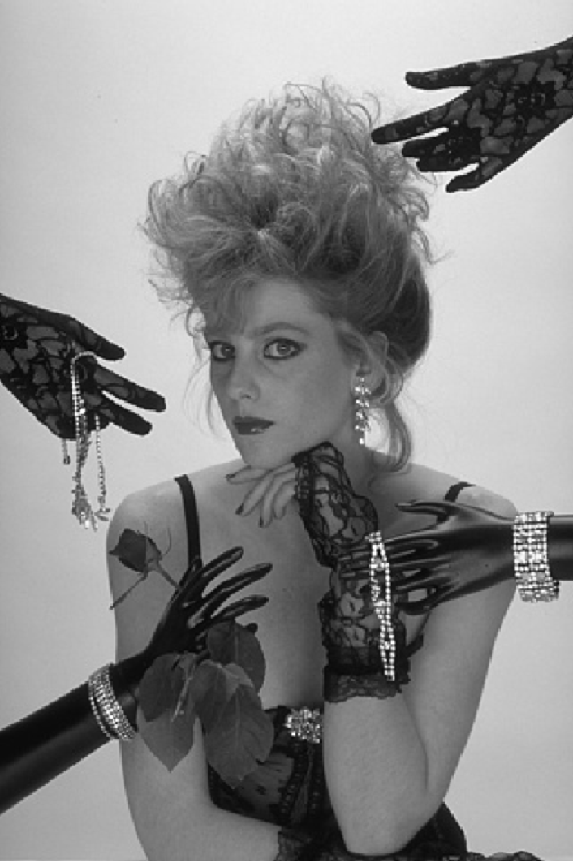
(a)

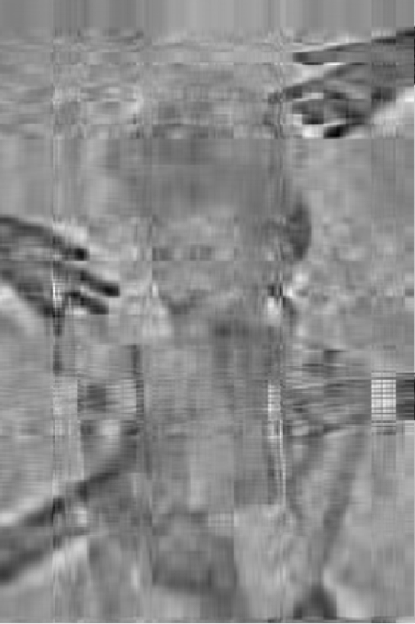
(b)

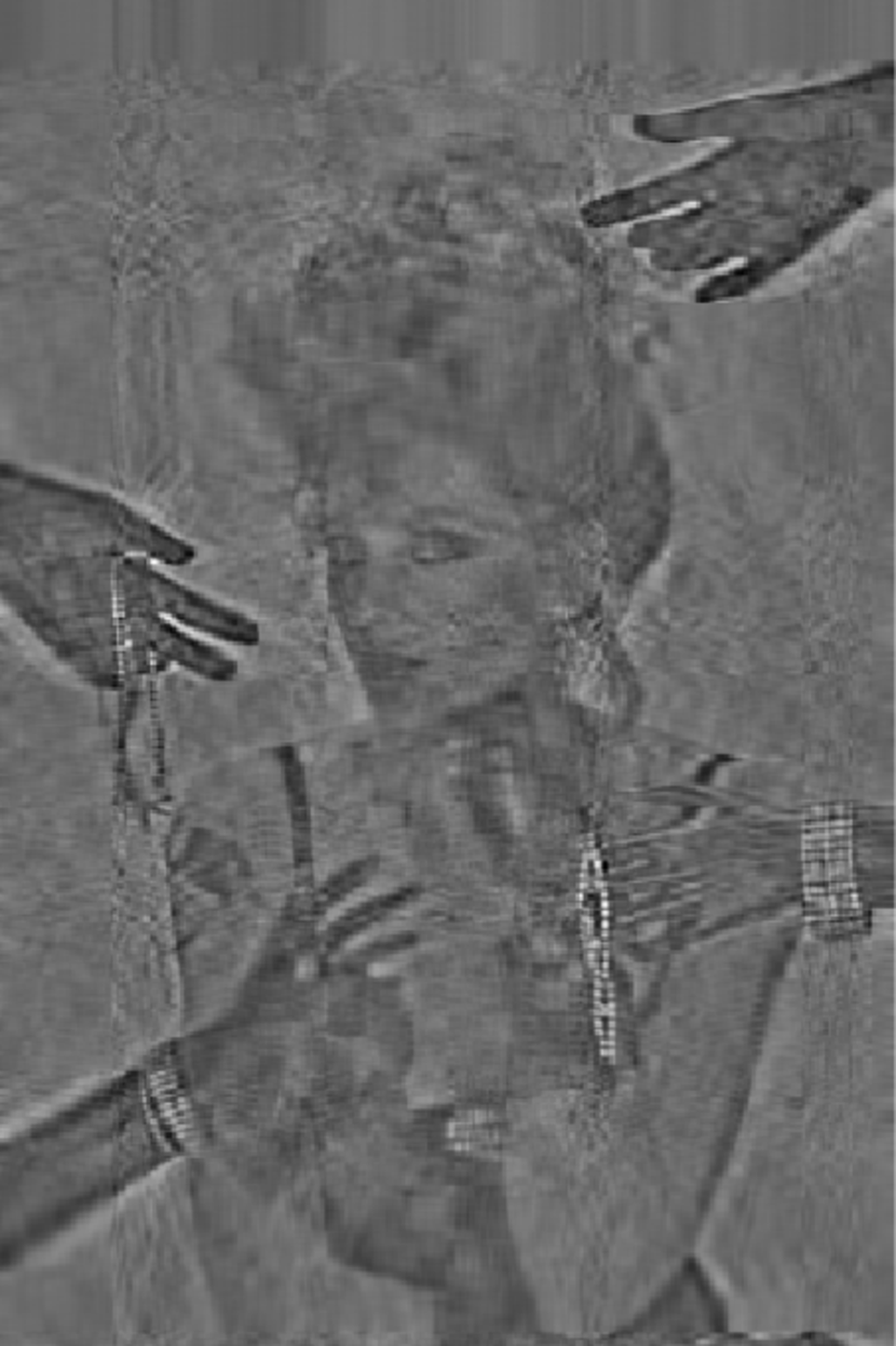
(c)

(d)

Figure 6: Ensemble images of Eq. 3 with different $k$ values: (a) Original image, (b) $k$=15, (c) $k$=40, (d) $k$=100

To develop an automatic predictor of the quality of generative images, we devised two different groups of features. We will refer to these as singular value decomposition (SVD) features and histogram-distance features. The former is designed to capture the structural similarity between an original and a test images while the latter is intended to measure the statistical similarity of the images.

IV-A SVD based Features for the Structural Similarity

Commonly used 2-D image transforms such as the DFT or DCT decompose an image using a fixed basis set. In principle, any structural degradation of a test image with respect to a reference image can be measured from changes in the transform coefficients. However, since the basis functions of SVD are unique to each image, changes in a test image can be measured both on an image’s basis set as well as the transform coefficients. For an $r\times c$ input image $X$, the SVD is defined as:

$$X=U\cdot\sigma\cdot V^{T}$$

where $U=[u_{1},u_{2},...,u_{r}]$ is an $r\times r$ left singular vector matrix, $V=[v_{1},v_{2},...,v_{c}]$ is a $c\times c$ right singular vector matrix, and $\sigma=diag(\sigma_{1},\sigma_{2},...,\sigma_{t})$ is a diagonal matrix of singular values in descending order: $\sigma_{1}>\sigma_{2},...>\sigma_{t}$ ($t$=min{$r$, $c$}).
Singular vectors and singular values contain useful information related to image structure and frequencies [50]. Given an SVD basis $u_{i}\cdot v_{i}^{T}$, then an ensemble image of accumulated basis images may be formed:

$$X_{k}=\sum_{i=1}^{k}u_{i}\cdot v_{i}^{T}$$ (3)

where $k\leq t$. Each basis implies a single layer of image structure while the sum of all layers yields the complete image structure. The first few layers contain the large-scale image structures, while the subsequent layers contain successive finer details in the image. An example is depicted in Fig. 6, portraying different ensemble images obtained with different $k$ values. When just the first few basis images are used ($k$=15), the large structures in the image begin to appear, while finer structural details emerge as the number $k$ of basis images is increased. The singular vectors, $u_{i}$ and $v_{j}$, capture the structural elements images, and may embody distortion-induced changes in them.
The singular values function weight their corresponding basis, and thereby represent the degree of luminance variation, strong textures versus smoothness or weak textures. For example, the ratio of the largest to the second largest singular value was used to estimate texture degree in [51]. Since different distortions may modify the luminance patterns of original images characteristically, it should be possible to likewise represent them in the singular values. In short, the singular vectors and the singular values allow the possibility of separately analyzing changes in structures and in luminance variation.

Figure 7: SVD sub-band division used to create ensemble image bands ($H<W$).

We utilize several SVD related features. Since each basis image contributes to an image’s structure/frequency content depending on the layer ordering, we divide the $U$ and $V$ matrices into three bands as shown in Fig. 7. Suppose that an input image of resolution $H$x$W$ is decomposed resulting in $U$ ($H$x$H$) and $V$ ($W$x$W$) matrices. Given $k$=min{$H$, $W$}, we use the first $\frac{1}{6}\cdot k$ singular vectors in $U_{LB}$ and $V_{LB}$ to construct a low band ensemble image ($EI_{LB}=U_{LB}\cdot V^{T}_{LB}$). Similarly, mid and high band ensembles images are constructed using the subsequent $\frac{2}{6}\cdot k$ and $\frac{3}{6}\cdot k$ singular vectors in $U_{MB}/V_{MB}$ and $U_{HB}/V_{HB}$, respectively. ($EI_{MB}=U_{MB}\cdot V^{T}_{MB}$ and $EI_{HB}=U_{HB}\cdot V^{T}_{HB}$).
The first feature is the sum of absolute differences between ensemble images for each sub-band as:

where $ER_{B}$ and $ET_{B}$ are from ensemble images of the reference image and a test image for band $B$ ($\in\{LB,MB,HB\}$), respectively. The second SVD related feature utilizes the eigen images $X_{k}=\sum_{i=1}^{k}u_{i}\cdot\sigma_{i}\cdot v_{i}^{T}$, then form the sum of absolute differences between the eigen images from each sub-band as:

where $R_{B}$ and $T_{B}$ are the eigen images of the reference and test images for band $B$. As discussed in [52], changes in an image’s structure can significantly affect the singular vectors, hence our third feature is defined as:

where $XR_{B}$ and $XT_{B}$ ($X\in\{U,V\}$) are the singular vector matrices of band B for the reference and test images, respectively, and $U_{B}$ and $V_{B}$ are the number of singular vectors in $UR_{B}$ and $VR_{B}$. The operation $\circ$ denotes the matrix inner product.
The last SVD feature is the sum of absolute differences of the singular values:

where $diagR_{B}$ and $diagT_{B}$ are the 1-D vectors of singular values in band $B$, of the reference and test images, respectively, and where $N_{B}$ is the number of singular values in band $B$.
The sub-bands for $F3^{B}_{svd}\sim F4^{B}_{svd}$ are divided into $\{LB,MB,HB\}$ in the same way as for $F1^{B}_{svd}$. Thus, the total number of SVD related features is 12 ($4$ features $\times 3$ bands).

IV-B Histogram Features

As discussed earlier, optimized GAN images may appear highly photorealistic, since both the semantics/structural and statistical/spectral/textural characteristics of the original image are well preserved. Although the local structure or detail may be slightly modified, preserving the statistical similarity yields a visually similar and a natural viewing experiences.
To quantify the degree of statistical similarity between reference and distorted images, we utilize a variety of histogram features. Begin with the coefficient of variation (CoV):

$$\rho=\frac{\sigma}{\mu},$$ (8)

where $\sigma$ and $\mu$ are the standard deviation and sample mean of a set of values, which will be drawn from both spatial and frequency domains. To derive the spatial features, first partition an image into 5x5 blocks. For example, 6,144 values of $\rho$ would be computed on a 480x320 image. Likewise, compute the 2-D DCT of each 5x5 block and compute (8) on it. Then construct histograms of the collected CoV values on both the reference image and the test image. Denote these histograms as $\rho_{ab}$, where $a\in\{s,f\}$ indicates spatial and frequency CoV values, and $b\in\{r,t\}$ indicates whether measured on reference or test image. Then, measure the distances between histograms $\rho_{rs}$ and $\rho_{ts}$ using the Kullback Leibler (KL) distance measures:

$$KL(\rho_{rs},\rho_{ts})=\sum_{i=1}^{N}\rho_{rs}(i)log\frac{\rho_{rs}(i)}{\rho_{ts}(i)}$$ (9)

where $\rho_{rs}(i)$ and $\rho_{ts}(i)$ are the $i$-th bin values of the spatial CoV histograms of the reference and test images, respectively. Similarly, define $KL(\rho_{rf},\rho_{tf})$ for the frequency CoV values. These distances become zero if the test image is the same as the reference image.

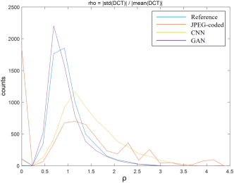
Figure 8: Histograms $\rho_{rf}$ and $\rho_{tf}$ as a function of $\rho$ for the four images in Fig. 1.

TABLE II: KL-distances between the distorted image histograms and the reference image histogram in Fig. 8

	JPEG-coded	CNN	GAN
KL-distance (of $F2_{hist}$) to reference	0.3710	0.2068	0.0182

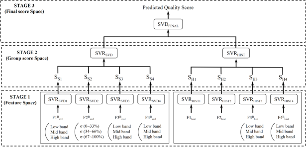
Figure 9: Block diagram of the 3-stage parallel boosting system.

Given these measurements, define the first and second histogram features in the intensity and frequency domains as:

$$F1_{hist}=KL(\rho_{rs},\rho_{ts})$$ (10)

$$F2_{hist}=KL(\rho_{rf},\rho_{tf})$$ (11)

Next, similar to the SVD based features, construct a set of ensemble images on which we define histogram features. Ensemble images for the three bands LB, MB and HB are constructed firstly, then the 2-D DCT is applied to them. The third and the fourth histogram features are expressed as KL distances in the space and frequency domains:

$$F3^{B}_{hist}=KL(Hist^{ER_{B}}_{space},Hist^{ET_{B}}_{space})$$ (12)

$$F4^{B}_{hist}=KL(Hist^{ER_{B}}_{dct},Hist^{ET_{B}}_{dct}).$$ (13)

In sum, there are eight histogram features in total.
Fig. 8 plots four curves representing the histograms ($\rho_{rf}$ and $\rho_{tf}$ in Eq. 11) of the four images in Fig. 1. The histogram curves show a good fit of the GAN image with the reference image, but poor fits of the CNN and JPEG-coded images. Table II lists the $KL$-distances of the distorted-image histograms to reference image histogram, reinforcing this result.

IV-C Block Feature Calculations

In addition to calculating features on entire frames, as explained in Sections IV-A & IV-B, we also compute features on a block-wise basis, which are then pooled to also produce whole image features. In this way, we are able to better capture local characteristics of distortions. However, this benefit would get weakened if the block size becomes too large or too small.
To analyze the relationship between block size and prediction accuracy, we performed some additional experiments. Table III shows the PCC/SRCC values obtained using 5-fold CV for different block sizes on the subset of full-frame images. For $F_{hist}$ features, the indicated block sizes were used for $\rho$ calculations, while the region over which the KL-distance calculation (in parentheses) increased accordingly. We found that block sizes of 10x10 and 5x5 for $F_{svd}$ and $F_{hist}$ provided the best prediction accuracy. These block feature values were then pooled by averaging them to produce the final feature indices. We provide assessments of the individual performance of the full-frame and block-based features in Section V.

TABLE III: Summary of results against block size on the subset of full-frame images.

$F_{svd}$			$F_{hist}$
Block Size	PCC	SROCC	Block Size	PCC	SROCC
5x5	0.837	0.841	5x5 (10x10)	0.947	0.903
10x10	0.947	0.903	10x10 (20x20)	0.871	0.822
20x20	0.852	0.827	25x25 (50x50)	0.878	0.809

IV-D Multi-stage Parallel Boosting System

To learn a highly nonlinear model between the MOS and the proposed features, we employed a 3-stage parallel boosting system as demonstrated in Fig. 9. In the first stage, nine individual feature sets were each used to train separately support vector regressor (SVR) to predict the MOS. In the second stage, four $F_{svd}$ related scores ($S_{S1}\sim S_{S4}$) and four $F_{hist}$ related scores ($S_{H1}\sim S_{H4}$) were fed into two corresponding SVRs, respectively, to further boost the prediction accuracy using the same group of feature scores. The final predicted image quality score was obtained from the third stage, which fuses the two group scores. This hierarchical structure boosted the prediction of the single feature by using the group scores. The boosted predictions were boosted further by using the across-group scores.
To be more concrete, the SVRs in stage I take $(\boldsymbol{x}_{n},y_{n})$ as a set of training data, where $\boldsymbol{x}_{n}$ is a feature vector and $y_{n}$ is the target label, e.g., the MOS of the $n$th image. We deploy $\varepsilon$-SVR [53], where the goal is to find a mapping function $f(\boldsymbol{x}_{n})$ having a deviation of no more than $\varepsilon$ from the target label $y_{n}$ over all the training data. The mapping function has the form:

$$f(\boldsymbol{x})=\boldsymbol{w_{f}}^{T}\phi(\boldsymbol{x})+b_{f},$$ (14)

where $\boldsymbol{w_{f}}$ is a weighting vector, $\phi(\cdot)$ is a non-linear function, and $b_{f}$ is a bias term. The subscript $f$ implies that the SVRs in Stage I operate in feature space, with feature vectors as input. It is desired to find $\boldsymbol{w}$ and $b$ satisfying the following condition:

$$|f(\boldsymbol{x}_{n})-y_{n}|\leq\varepsilon,\quad\forall n=1,2,\ldots,N_{t},$$ (15)

where $N_{t}$ is the number of training data. We use the radial basis activation function (RBF), since it provides good performance in many image quality prediction applications [14, 15, 41]. Since it is challenging to determine a proper value of $\varepsilon$ in (15), we used a modified version of the regression algorithm called $\nu$-SVR [54], where $\nu\in(0,1)$ is a control parameter to adjust the number of support vectors and the accuracy level. Then, $\varepsilon$ becomes a variable to be optimized, and we obtained $f(\boldsymbol{x})$ and $\boldsymbol{w}$ more easily.
In Stage II and III, we fused all of the intermediate scores from the previous stage to determine a final predicted quality score. Suppose that there are $n$ SVRs fed by $m$ training images. On the $i$th image, compute the intermediate score $s_{i,j}$, where $i=1,2,...,m$ indexes the training images and $j=1,2,...,n$ is SVR index. Let $\boldsymbol{s}_{i}=(s_{i,1},s_{i,2},\cdots,s_{i,n})$ be the intermediate score vector for the $i$th image. We trained the SVRs using $\boldsymbol{s_{i}}$ using all the images in the training set, and determined the weight vector $\boldsymbol{w_{s}}$ and bias parameter $b_{s}$ accordingly. The subscript $s$ indicates that the SVRs operate in score space with the intermediate score vectors as input. Finally, the ultimate designed image quality model was found:

$$Q(\boldsymbol{s})=\boldsymbol{w_{s}}^{T}\phi(\boldsymbol{s})+b_{s}.$$ (16)

TABLE IV: Performances of single features on the proposed generative image database.

Feature Group	Feature	Sub-band	Subset of Full-Frame Images						Subset of Randomly Structured Block Patches						Subset of Regular Structured Block Patches						Subset of High-level Structured Block Patches
			Full-frame Features			Block Average Features			Full-frame Features			Block Average Features			Full-frame Features			Block Average Features			Full-frame Features			Block Average Features
			PCC	SROCC	RMSE	PCC	SROCC	RMSE	PCC	SROCC	RMSE	PCC	SROCC	RMSE	PCC	SROCC	RMSE	PCC	SROCC	RMSE	PCC	SROCC	RMSE	PCC	SROCC	RMSE
SVD based Feature	$F1^{B}_{svd}$	LB	0.61	0.60	5.11	0.66	0.65	4.84	0.65	0.70	5.07	0.64	0.62	5.14	0.90	0.89	2.65	0.72	0.70	4.28	0.91	0.92	2.97	0.92	0.90	3.08
		MB	0.55	0.52	5.42	0.46	0.48	6.48	0.55	0.59	5.56	0.42	0.31	6.05	0.83	0.83	3.44	0.75	0.73	4.06	0.82	0.80	4.10	0.78	0.80	7.22
		HB	0.19	0.41	6.36	0.17	0.33	6.39	0.26	0.21	6.44	0.54	0.52	5.62	0.49	0.47	5.37	0.28	0.05	5.92	0.30	0.31	6.92	0.25	0.05	6.99
	$F2^{B}_{svd}$	0-33%	0.31	0.39	6.15	0.61	0.61	6.48	0.24	0.11	6.49	0.42	0.41	6.68	0.45	0.48	5.49	0.76	0.76	3.98	0.27	0.52	6.95	0.64	0.62	7.22
		34-66%	0.54	0.58	5.45	0.30	0.28	6.48	0.55	0.48	5.57	0.37	0.47	6.23	0.74	0.71	4.17	0.38	0.40	6.16	0.69	0.64	5.25	0.36	0.32	7.22
		67-100%	0.42	0.37	5.87	0.38	0.29	5.99	0.19	0.21	6.59	0.28	0.27	6.40	0.78	0.78	3.89	0.72	0.71	4.26	0.76	0.75	4.72	0.58	0.61	7.22
	$F3^{B}_{svd}$	LB	0.65	0.64	4.93	0.65	0.64	4.94	0.68	0.67	4.90	0.63	0.61	5.18	0.86	0.82	3.42	0.71	0.71	4.33	0.89	0.87	3.25	0.84	0.83	3.86
		MB	0.56	0.54	5.36	0.61	0.59	5.12	0.58	0.57	5.42	0.64	0.66	5.15	0.83	0.85	3.10	0.80	0.79	3.73	0.81	0.80	4.24	0.90	0.92	2.81
		HB	0.24	0.27	6.30	0.56	0.53	5.36	0.32	0.28	6.32	0.68	0.65	4.87	0.38	0.37	5.70	0.79	0.76	3.79	0.29	0.32	6.91	0.76	0.74	4.72
	$F4^{B}_{svd}$	LB	0.50	0.45	5.62	0.69	0.68	6.48	0.11	0.14	6.64	0.25	0.26	6.68	0.35	0.32	5.77	0.54	0.57	6.16	0.35	0.30	6.75	0.51	0.52	7.22
		MB	0.51	0.44	5.59	0.60	0.62	6.48	0.55	0.51	5.58	0.64	0.68	6.68	0.59	0.56	4.98	0.73	0.76	6.16	0.43	0.42	6.50	0.62	0.62	7.22
		HB	0.43	0.44	5.85	0.43	0.45	6.48	0.69	0.68	4.91	0.65	0.69	6.68	0.65	0.62	4.70	0.71	0.71	6.16	0.45	0.44	6.45	0.41	0.42	7.22
Histogram- distance based Feature	$F1_{hist}$		0.30	0.39	6.48	0.55	0.55	6.48	0.44	0.40	6.68	0.56	0.56	6.68	0.32	0.42	6.16	0.61	0.61	4.90	0.37	0.37	7.22	0.65	0.67	7.22
	$F2_{hist}$		0.44	0.47	5.81	0.33	0.43	6.48	0.71	0.70	4.81	0.32	0.32	6.68	0.58	0.59	6.16	0.79	0.80	6.16	0.42	0.37	6.55	0.41	0.40	7.22
	$F3^{B}_{hist}$	LB	0.45	0.33	6.48	0.04	0.10	6.48	0.56	0.51	6.68	0.39	0.44	6.68	0.29	0.12	6.16	0.67	0.66	6.16	0.40	0.34	7.22	0.63	0.58	7.22
		MB	0.31	0.38	6.48	0.03	0.07	6.48	0.54	0.37	6.68	0.08	0.00	6.68	0.31	0.09	6.16	0.20	0.16	6.16	0.37	0.30	7.22	0.26	0.22	7.22
		HB	0.40	0.33	6.48	0.26	0.32	6.48	0.41	0.46	6.68	0.39	0.37	6.68	0.33	0.19	6.16	0.18	0.10	6.16	0.44	0.53	7.22	0.14	0.16	7.22
	$F4^{B}_{hist}$	LB	0.47	0.56	6.48	0.12	0.15	6.48	0.75	0.74	4.45	0.17	0.22	6.68	0.47	0.44	6.16	0.61	0.60	6.16	0.43	0.31	6.51	0.42	0.41	7.22
		MB	0.29	0.35	6.48	0.28	0.35	6.22	0.59	0.56	5.38	0.25	0.41	6.47	0.45	0.34	5.49	0.10	0.08	6.16	0.32	0.30	7.22	0.32	0.38	6.85
		HB	0.33	0.49	6.48	0.11	0.38	6.48	0.47	0.48	6.68	0.20	0.24	6.68	0.37	0.27	6.16	0.41	0.56	5.61	0.45	0.45	7.22	0.50	0.43	6.24

For the performance evaluation, we split the dataset into two training and testing subsets, consisting of 80% and 20% of the entire collection of images, respectively. The images in the training and testing subsets were drawn from non-overlapping content to avoid the SVRs learning the images. The SVRs were trained on the training set, and the learned models were then tested on the testing set. To ensure that the proposed IQA model is robust across contents and was not dominated by the specific train-test split, we repeated this random split 1000 times on the dataset, and recorded the performances on each of the test sets. For all of the experiment results, we reported the median values across these 1000 train-test iterations as performance indices. In addition, feature normalization was performed prior to the training and test processes, to avoid features having larger numeric ranges dominating those having smaller numeric ranges. We scaled the input of each SVR to the unit range [0,1] using $(val–MIN)/(MAX-MIN)$. During the training stage, the goal was to determine the optimal weighting vector $\boldsymbol{w}$ and bias $b$ minimizing the error between the MOS and the predicted scores:

$$\sum_{i}|\mbox{MOS}_{i}-Q(\boldsymbol{s}_{i})|^{2}.$$ (17)

Since we adopted the RBF kernel, the error penalty term ($C$) and the kernel parameter ($\gamma$) were optimized to achieve the highest accuracy. We searched the optimal $C$ and $\gamma$ during the training stage using the cross validation scheme in Section 3.2 of [55]. Specifically, we used the built-in training function in LIBSVM, which provides an option (-v) for running v-fold CV. Various $(C,\gamma)$ pairs were tried, and the one yielding the highest cross validation accuracy was selected. Finally, the entire training set was used again to generate the final SVR predictor. At the test stage, we use the intermediate score vector $s_{i}$ in (16) to determine the predicted score. The score prediction was quite fast, since all of the model parameters were decided during the training stage.

V Performance Evaluation and Analysis

Following the suggestions in ITU-T (p.1401) [56], we used three measures to evaluate the performance of the proposed image quality predictor: (1) the Pearson correlation coefficient (PCC) measures the linear relationship between a model’s score and the subjective data, (2) the Spearman rank-order correlation coefficient (SRCC), which measures the prediction monotonicity, and (3) the root mean squared error (RMSE), which quantifies the prediction accuracy. We apply the monotonic logistic function to the predicted scores to account for nonlinearity when fitting the subjective scores, but we did not apply the nonlinearity when computing the rank order correlation. The logistic function has the form:

$$L(s)=\frac{\beta_{1}-\beta_{2}}{1+exp(\frac{-s+\beta_{3}}{|\beta_{4}|})}+\beta_{2}$$ (18)

where $s$ and $L(s)$ are the predicted scores and the adjusted predicted scores, respectively, and $\beta_{k}$ ($k$ = 1,2,3,4) are the parameters that minimize the mean squared error between $L(s)$ and MOS. The choices of the initial parameters are explained in [57].

V-A Performance Analysis on Individual Features

TABLE V: Performance comparison on the proposed generative image database (median PCC, SRCC and RMSE across 1,000 train-test trials for $SSQP_{F}$ and $SSQP_{B}$)

. Full-Frame Images Randomly Structured Patches Regular Structured Patches High-level Structured Patches PCC SROCC RMSE PCC SROCC RMSE PCC SROCC RMSE PCC SROCC RMSE PSNR 0.58 0.56 5.29 0.43 0.41 6.04 0.78 0.79 3.87 0.72 0.75 4.99 SSIM 0.60 0.59 5.18 0.62 0.60 5.26 0.85 0.85 3.21 0.77 0.79 4.57 MSIM 0.74 0.74 4.32 0.68 0.70 4.90 0.76 0.77 4.03 0.84 0.80 3.96 VSNR 0.67 0.67 4.82 0.66 0.60 5.00 0.64 0.65 4.71 0.77 0.75 4.63 VIF 0.81 0.79 3.77 0.69 0.60 4.85 0.84 0.85 3.34 0.90 0.88 3.20 VIFP 0.67 0.66 4.80 0.68 0.56 4.90 0.77 0.78 3.91 0.84 0.82 3.95 UQI 0.71 0.69 4.58 0.61 0.60 5.27 0.71 0.69 4.32 0.81 0.80 4.28 IFC 0.79 0.76 4.00 0.66 0.66 4.99 0.82 0.83 3.50 0.90 0.90 3.10 NQM 0.57 0.55 5.32 0.57 0.54 5.49 0.71 0.68 4.32 0.88 0.85 3.42 WSNR 0.53 0.51 5.48 0.53 0.59 5.66 0.52 0.51 5.25 0.59 0.57 5.85 SNR 0.54 0.51 5.47 0.28 0.25 6.42 0.72 0.72 4.25 0.72 0.68 5.00 FSIM 0.84 0.82 3.54 0.70 0.65 4.78 0.93 0.91 2.33 0.88 0.88 3.41 GMSD 0.89 0.88 6.48 0.71 0.65 6.68 0.80 0.80 6.16 0.87 0.88 7.22 $SSQP_{F}$ 0.93 0.88 2.32 0.91 0.86 2.44 0.96 0.88 1.54 0.96 0.90 1.87 $SSQP_{B}$ 0.95 0.89 2.03 0.87 0.81 2.84 0.95 0.88 1.70 0.94 0.86 2.13

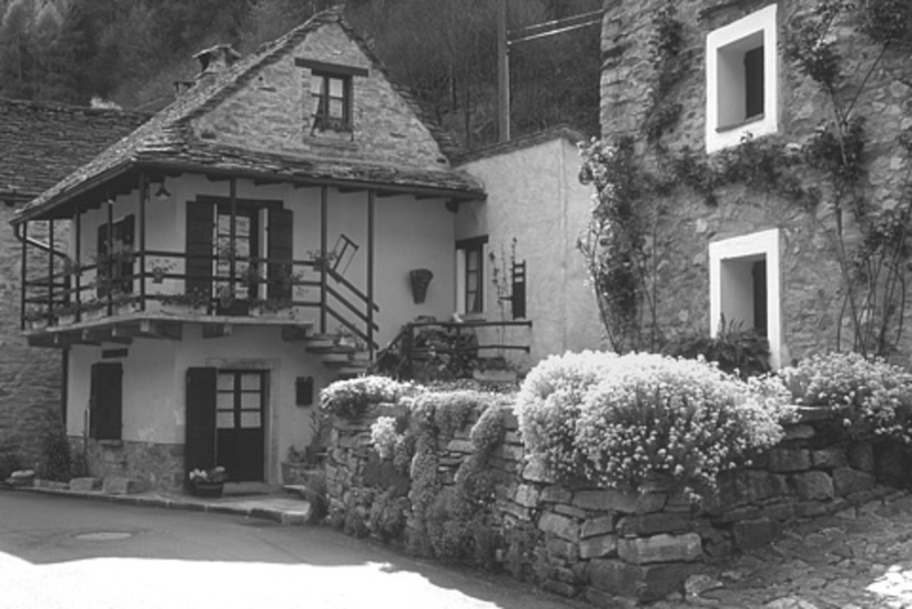
(a)

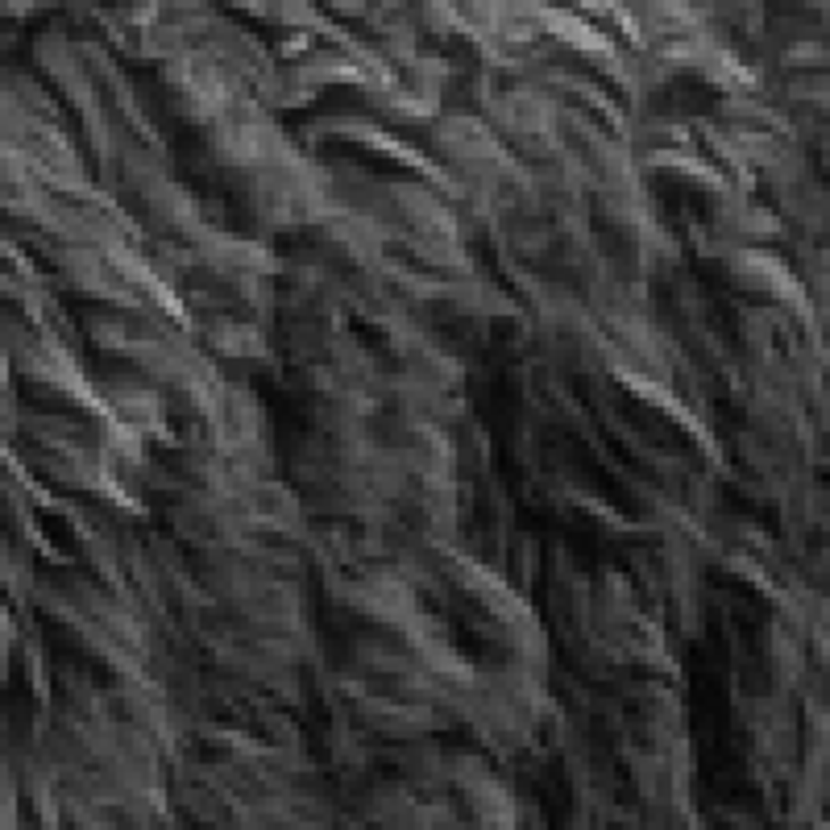
(b)

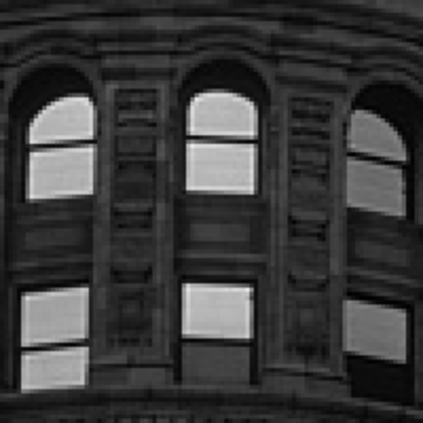
(c)

(d)

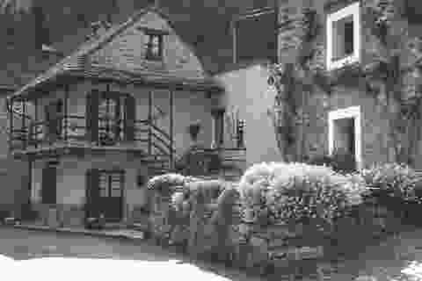
(e)

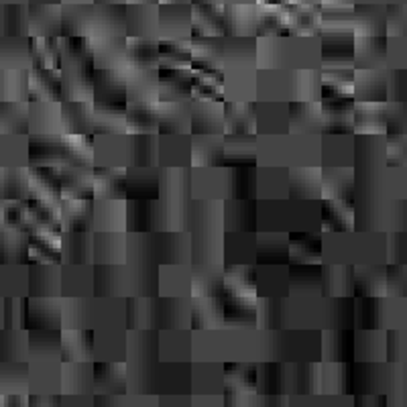
(f)

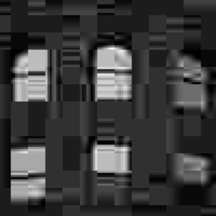
(g)

(h)

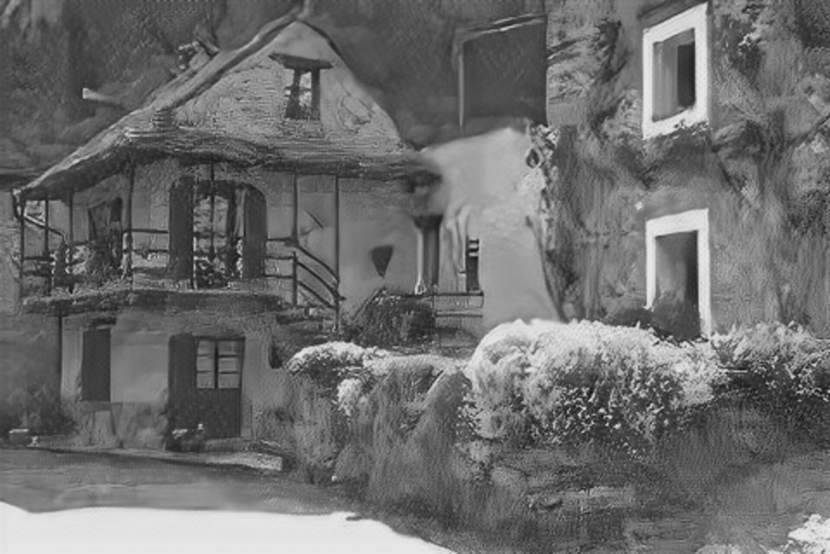
(i)

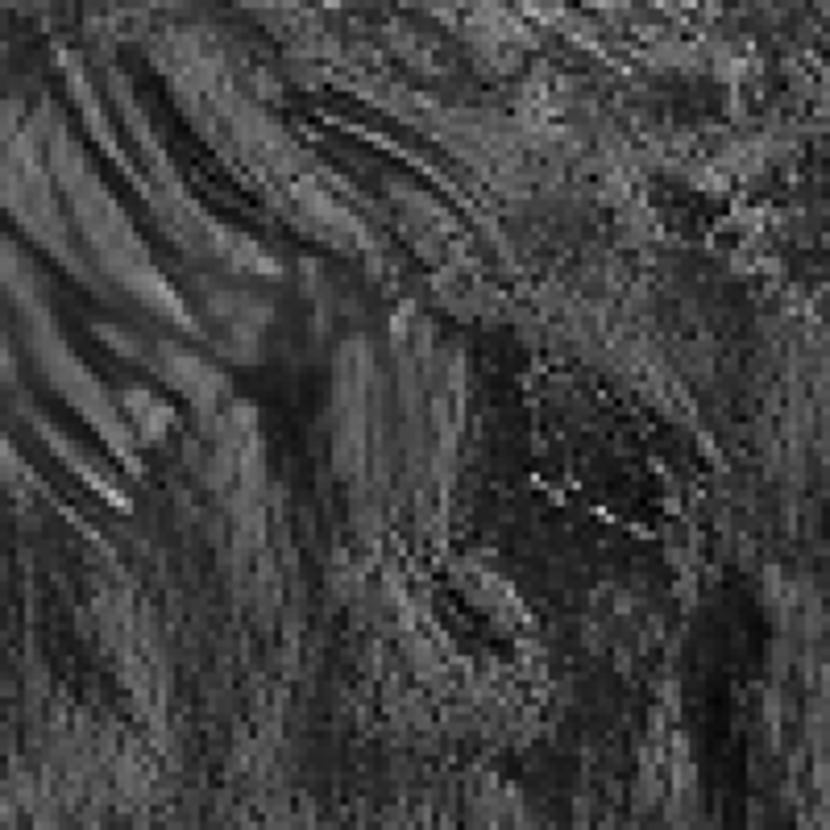
(j)

(k)

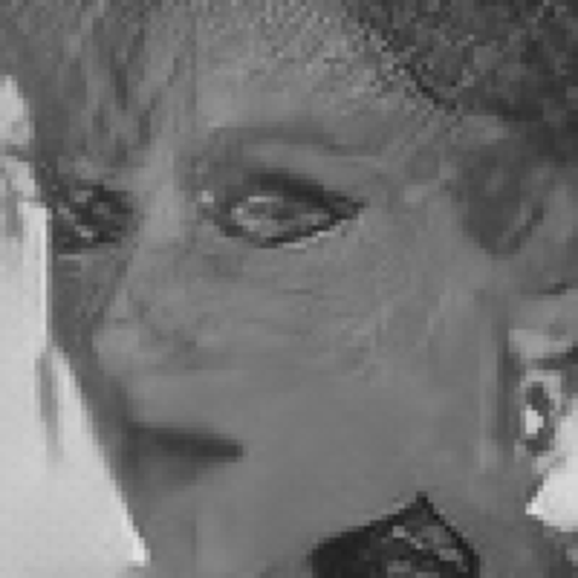
(l)

Figure 10: The subjective quality comparison: (a) House image from subset of full-frame images, (b) Llama fur patch from subset of random structured patches, (c) building patch from subset of regular structured patches, (d) face patch from subset of high-level structured patches, (e)-(h): the corresponding JPEG QF05 images, (i)-(l): the corresponding GAN images ($\lambda$=0.1 with input of JPEG QF05).

Next, we analyze the performance of each individual feature on the proposed generative image database, which consists of four sub-datasets. Table IV lists the experimental results on all the sub-datasets, where the three top-performing features in each index are marked in bold. In the following analysis, the designation $F$ or $B$ means that the feature is calculated on full frames or is a block average, respectively.
For the first subset of full-frame images, the SVD related features, such as $F3^{LB}_{svd_{F}}$ (PCC=0.65) and $F1^{LB}_{svd_{F}}$ (PCC=0.61) (full-frame features) and $F5^{LB}_{svd_{B}}$ (PCC=0.69) and $F1^{LB}_{svd_{B}}$ (PCC=0.66) (block average features) yielded good performance. In general, the block average based features provided better performance than did the full-frame based features. Also, the low band features yielded better predictors than those from the mid and high bands, probably because preservation of the overall image structure is more important than retaining fine details on full-frame generative images. The histogram-distance based features yielded relatively low prediction accuracy on this subset.
For the second subset of randomly structured patches, meaningful differences as compared to the previous subset were observed. The histogram-distance based features delivered improved performance, possibly due to the reasons explained in Section IV-B. For example, $F4^{LB}_{hist_{F}}$ gave the best PCC value (0.75). The block-average features also provided performance increases, but not as good as the full-frame based features, possibly because the fixed block sizes (10x10/20x20) restricted performance as compared to full-frame calculation. Among the SVD related features, $F3^{HB}_{svd_{B}}$ (0.68) and $F5^{HB}_{svd_{F}}$ (0.69) also delivered high prediction accuracy, perhaps because the high band captures high frequency image and distortion details, which strongly characterize the second subset. The results on the subset of regular structured patches strongly suggest that structure-representing features are well correlated with MOS. For example, $F1^{LB}_{svd_{F}}$ (PCC=0.90) and $F3^{LB}_{svd_{F}}$ (PCC=0.86) yielded very good predictions. Lastly, on the subset of high-level structured patches, the same tendency was observed, and $F1^{LB}_{svd_{B}}$ (PCC=0.92) and $F1^{LB}_{svd_{F}}$ (PCC=0.91) yielded very good prediction performance.
In sum, the single feature analysis showed that the SVD-related features effectively captured the similarities in structure, while the histogram-distance related features were more useful for representing statistical similarities.

V-B Algorithm Comparison on the Generative IQA Database

TABLE VI: Experimental results on four selected test image sets: In each row, two test images are highlighted which obtained the highest and the lowest scores in green and red, respectively.

House Image from the Subset of Full-frame Images													Llama Fur patch from the Subset of Randomly Structured Patches
Metric	JPEG			CNN			GAN (lambda=0.1)			GAN (lambda=0.01)			Metric	JPEG			CNN			GAN (lambda=0.1)			GAN (lambda=0.01)
	QF05	QF10	QF20	QF05	QF10	QF20	QF05	QF10	QF20	QF05	QF10	QF20		QF05	QF10	QF20	QF05	QF10	QF20	QF05	QF10	QF20	QF05	QF10	QF20
PSNR	22.68	24.61	26.46	23.82	25.71	27.64	20.40	23.06	24.69	20.94	23.62	25.07	PSNR	22.862	25.100	27.265	23.935	26.268	28.572	20.176	24.895	25.466	21.563	23.762	26.922
SSIM	0.57	0.70	0.80	0.62	0.73	0.83	0.47	0.64	0.73	0.47	0.65	0.77	SSIM	0.521	0.684	0.809	0.555	0.716	0.838	0.369	0.682	0.741	0.415	0.626	0.782
MSIM	0.87	0.94	0.97	0.89	0.95	0.97	0.83	0.92	0.96	0.84	0.92	0.96	MSIM	0.827	0.923	0.966	0.843	0.931	0.971	0.787	0.919	0.959	0.776	0.895	0.960
VSNR	18.89	22.87	27.46	20.38	24.15	28.70	16.97	21.54	25.85	17.25	21.76	25.06	VSNR	9.477	13.647	18.055	10.569	14.430	19.242	8.073	14.114	17.252	8.772	13.872	17.143
VIF	0.17	0.30	0.47	0.21	0.34	0.50	0.15	0.29	0.43	0.16	0.28	0.44	VIF	0.128	0.260	0.427	0.145	0.286	0.452	0.101	0.257	0.402	0.103	0.237	0.406
VIFP	0.21	0.30	0.39	0.26	0.35	0.44	0.17	0.28	0.35	0.18	0.28	0.38	VIFP	0.151	0.256	0.352	0.180	0.289	0.389	0.110	0.257	0.301	0.115	0.225	0.330
UQI	0.47	0.63	0.75	0.51	0.65	0.77	0.38	0.57	0.68	0.40	0.58	0.71	UQI	0.523	0.707	0.828	0.545	0.732	0.855	0.386	0.701	0.769	0.416	0.636	0.802
IFC	1.53	2.71	4.28	1.87	3.10	4.69	1.36	2.57	3.93	1.41	2.55	4.07	IFC	0.904	1.861	3.116	1.055	2.081	3.345	0.710	1.852	2.917	0.739	1.718	2.994
NQM	17.39	23.48	28.96	19.14	24.46	29.54	12.94	20.63	23.13	15.07	21.04	20.41	NQM	3.232	5.827	8.620	4.358	7.173	10.171	1.272	6.181	7.367	2.381	5.723	8.648
WSNR	25.16	30.82	36.42	26.67	31.68	37.07	19.86	27.59	28.88	21.34	27.20	25.56	WSNR	18.157	23.618	29.022	19.090	24.177	29.402	16.009	20.130	25.522	16.518	16.698	25.584
SNR	16.02	17.95	19.80	17.16	19.05	20.98	13.74	16.40	18.03	14.28	16.96	18.41	SNR	10.883	13.121	15.285	11.956	14.289	16.593	8.197	12.916	13.487	9.583	11.783	14.943
FSIM	0.77	0.85	0.90	0.79	0.87	0.92	0.80	0.87	0.90	0.80	0.86	0.91	FSIM	0.780	0.860	0.914	0.761	0.860	0.917	0.780	0.856	0.899	0.761	0.840	0.891
GMSD	0.18	0.09	0.04	0.13	0.08	0.04	0.14	0.09	0.05	0.13	0.09	0.04	GMSD	0.148	0.076	0.040	0.139	0.070	0.034	0.137	0.080	0.045	0.142	0.090	0.044
$SSQP_{F}$	1.45	5.65	15.78	2.84	8.98	15.24	1.65	17.69	18.98	2.40	16.62	18.34	$SSQP_{F}$	0.79	11.45	15.78	7.10	8.40	17.75	2.12	4.53	15.68	4.01	13.23	17.89
$SSQP_{B}$	1.37	5.01	18.47	2.10	11.06	17.81	2.63	15.04	18.73	2.22	12.30	17.64	$SSQP_{B}$	1.86	12.23	18.66	3.87	14.32	18.81	2.51	12.53	12.50	2.19	4.47	19.61
MOS	0.00	5.88	12.38	2.63	11.00	14.75	3.25	15.13	18.00	3.50	13.00	16.25	MOS	0.00	0.50	8.38	5.13	9.38	18.00	4.88	13.13	17.63	8.00	15.25	18.63
Building patch from the Subset of Regular Structured Patches													Face patch from the Subset of High-level Structured Patches
Metric	JPEG			CNN			GAN (lambda=0.1)			GAN (lambda=0.01)			Metric	JPEG			CNN			GAN (lambda=0.1)			GAN (lambda=0.01)
	QF05	QF10	QF20	QF05	QF10	QF20	QF05	QF10	QF20	QF05	QF10	QF20		QF05	QF10	QF20	QF05	QF10	QF20	QF05	QF10	QF20	QF05	QF10	QF20
PSNR	23.183	25.958	28.455	26.299	29.424	31.954	21.087	26.364	27.776	23.912	26.218	29.805	PSNR	25.414	27.890	30.193	26.995	29.857	32.168	23.907	26.703	29.299	24.385	27.874	29.267
SSIM	0.598	0.764	0.857	0.692	0.838	0.909	0.482	0.766	0.849	0.586	0.749	0.871	SSIM	0.704	0.795	0.868	0.791	0.870	0.910	0.627	0.711	0.824	0.619	0.782	0.872
MSIM	0.902	0.956	0.981	0.925	0.969	0.987	0.860	0.956	0.979	0.898	0.948	0.981	MSIM	0.882	0.944	0.976	0.907	0.965	0.982	0.817	0.932	0.958	0.838	0.938	0.970
VSNR	21.122	26.609	32.235	24.829	30.120	35.915	18.117	27.438	30.820	21.986	26.756	32.506	VSNR	18.325	22.985	27.589	20.081	25.222	29.897	16.721	22.330	25.900	17.618	22.721	27.157
VIF	0.223	0.375	0.533	0.304	0.466	0.609	0.215	0.385	0.542	0.250	0.379	0.544	VIF	0.183	0.316	0.477	0.239	0.386	0.532	0.174	0.328	0.460	0.184	0.320	0.475
VIFP	0.249	0.359	0.455	0.348	0.468	0.565	0.213	0.382	0.474	0.275	0.371	0.488	VIFP	0.223	0.346	0.460	0.301	0.438	0.534	0.186	0.327	0.408	0.187	0.343	0.460
UQI	0.545	0.745	0.852	0.607	0.804	0.898	0.436	0.733	0.840	0.508	0.695	0.855	UQI	0.443	0.624	0.755	0.550	0.710	0.801	0.378	0.574	0.686	0.400	0.604	0.730
IFC	1.556	2.644	3.865	2.168	3.367	4.547	1.500	2.738	3.941	1.749	2.728	3.986	IFC	0.899	1.568	2.470	1.288	2.061	2.942	0.859	1.630	2.372	0.910	1.606	2.517
NQM	10.265	13.606	16.828	13.582	17.215	20.296	8.901	14.591	17.416	11.361	14.378	18.235	NQM	9.296	12.192	15.191	11.171	14.454	17.289	8.289	11.657	14.301	8.948	12.491	15.305
WSNR	19.850	25.593	30.892	22.418	27.117	32.003	15.938	21.888	22.089	19.493	20.919	28.291	WSNR	24.920	30.330	35.278	25.937	31.936	36.152	21.387	27.221	29.293	22.530	28.165	27.267
SNR	12.706	15.481	17.977	15.821	18.947	21.476	10.609	15.886	17.299	13.434	15.741	19.327	SNR	18.950	21.426	23.729	20.531	23.394	25.704	17.443	20.240	22.836	17.921	21.410	22.803
FSIM	0.795	0.846	0.899	0.825	0.908	0.947	0.786	0.888	0.930	0.819	0.882	0.932	FSIM	0.800	0.876	0.921	0.867	0.913	0.940	0.826	0.882	0.922	0.844	0.897	0.930
GMSD	0.170	0.098	0.051	0.148	0.082	0.038	0.146	0.096	0.051	0.161	0.104	0.050	GMSD	0.136	0.070	0.035	0.109	0.053	0.027	0.118	0.072	0.042	0.116	0.070	0.037
$SSQP_{F}$	0.51	3.10	12.67	4.27	15.08	17.90	0.70	9.01	16.12	2.70	6.34	16.75	$SSQP_{F}$	1.15	7.49	16.13	1.45	14.86	14.86	4.84	2.30	16.36	1.67	8.53	13.98
$SSQP_{B}$	1.32	6.81	14.19	10.85	15.84	17.04	1.54	8.02	16.54	5.39	6.86	17.27	$SSQP_{B}$	1.32	6.81	14.19	10.85	15.84	17.27	1.43	8.02	16.54	5.39	6.86	17.73
MOS	0.00	5.25	8.75	5.63	11.50	16.50	2.00	13.88	17.75	4.88	13.38	18.38	MOS	0.25	5.00	11.25	1.75	16.13	19.50	2.00	10.13	16.63	1.38	13.63	20.75

We call the proposed IQA model the $SSQP$ (Structural and Statistical Quality Predictor), and compared its performance against many leading 2D FR IQA models on the new generative image database. The experimental results are summarized in Table V. Note that $SSQP_{F}$ and $SSQP_{B}$ are two versions of $SSQP$ depending on the feature calculation method. The thirteen existing models that were used for performance benchmarking are PSNR, SSIM [30], multi-scale SSIM index (MSSIM) [31], visual signal-to-noise ratio (VSNR) [58], visual information fidelity (VIF) [59], pixel-based VIF (VIFP), universal quality index (UQI) [60], information fidelity criterion (IFC) [61], noise quality measure (NQM) [62], weighted signal-to-noise ratio (WSNR), signal-to-noise ratio (SNR), feature similarity index (FSIM) [63], and gradient magnitude similarity deviation (GMSD) [64]. The parameters used in each were the default settings mentioned in their original papers.
Table V shows that $SSQP$ significantly outperformed all of the compared FR on the subset of full-frame images, $SSQP_{B}$ and $SSQP_{F}$ achieved PCC=0.95 and PCC=0.93 while the best performance of a previously existing FR metric was GMSD with PCC=0.89. Note that as compared to performance on well-known image quality databases such as LIVE [40] and TID [65], where several state-of-the-art 2D FR metrics have already achieved excellent performance ($>0.95$ in PCC), the best PCC value achieved by any of the existing models on the new database was below 0.90, reflecting the more challenging aspects of the new data resource. On the subset of random structured blocks, the performance gap between $SSQP$ and the best existing models was even larger. Specifically, the PCC values attained by $SSQP_{B}$ and $SSQP_{F}$ were 0.91 and 0.87, respectively, whereas that of GMSD was 0.71. This could be because that most existing benchmark FR IQA models lack the ability to capture the requisite types of statistical similarity. The prediction accuracy of $SSQP$ improves even further (PCC=0.96 for $SSQP_{F}$) on the subset of regular structured patches and PCC=0.96 for $SSQP_{F}$ on the subset of high-level structured patches, while the best existing models were FSIM (PCC=0.93) and IFC (PCC=0.90), respectively. Overall, $SSQP_{B}$ was a better predictor than $SSQP_{F}$ because it was better able to account for the diversity of local characteristics in images.
In order to better understand the superiority of $SSQP$, we analyzed the limitations of the existing models. Fig. 10 show the four reference images from all the subsets and their corresponding JPEG QF05 images and $GAN$ images ($\lambda=0.1$ with input of JPEG QF05). Table VI shows the prediction performances of the benchmark models as well as their MOS. For each model, we highlighted two test images that caused the best and the worst scores in green and red, respectively. As shown in the results, most of the existing models selected CNN (with input of JPEG Q20) as the highest quality image and $GAN$ ($\lambda$=0.1 with input of JPEG QF05) as the worst. However, this was not always the case. In Table VI, the subjective scores indicate that JPEG QF05 was the worst image while $GAN$ ($\lambda$=0.1 with input of JPEG QF20) was the best image among the given examples. One likely reason for the inaccuracies of the existing metrics is that they aim to assess preservation of pixel-wise fidelity, rather than innate quality. This could explain why they tolerate severe blocking artifacts, but not moderate structural changes, even though the former are more annoying. This might explain why the existing models choose CNN-generated images rather than $GAN$ images as higher quality. However, CNN images introduce blur (as in Fig. 1(c)), which deteriorates the viewing experience. $SSQP$ evaluates the natural quality based on both structural and statistical similarities, which are not as strongly affected by pixel-wise differences. Moreover, the parallel boosting system is able to optimize the relative weights by considering the significance of the structural degradations against statistical degradations. This was experimentally verified in Table VI, where the $SSQP$ objective scores closely fit the MOS.

TABLE VII: Percentages of the worst and best case matches bewteen $SSQP_{B}$ and MOS.

Percentage of matches on lowest MOS images	Percentage of matches on highest MOS images
83.3% (15/18)	27.8% (5/18)

TABLE VIII: Distributions of highest MOS and $SSQP_{B}$ predictions against method of image generation.

	# of images having the highest score
Input image	CNN w/ QF20	GAN w/ QF20 ($\lambda=0.1$)	GAN w/ QF20 ($\lambda=0.01$)
MOS	1	13	4
$SSQP_{B}$	3	2	13

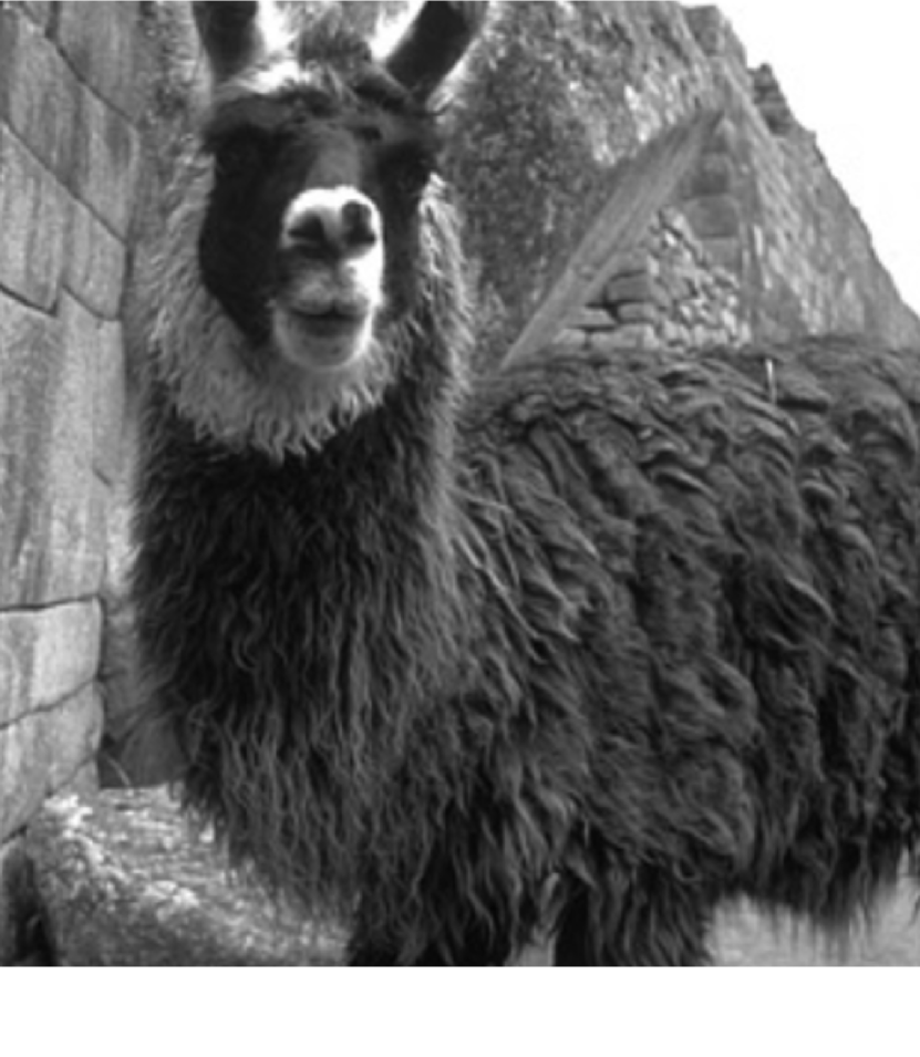
(a)

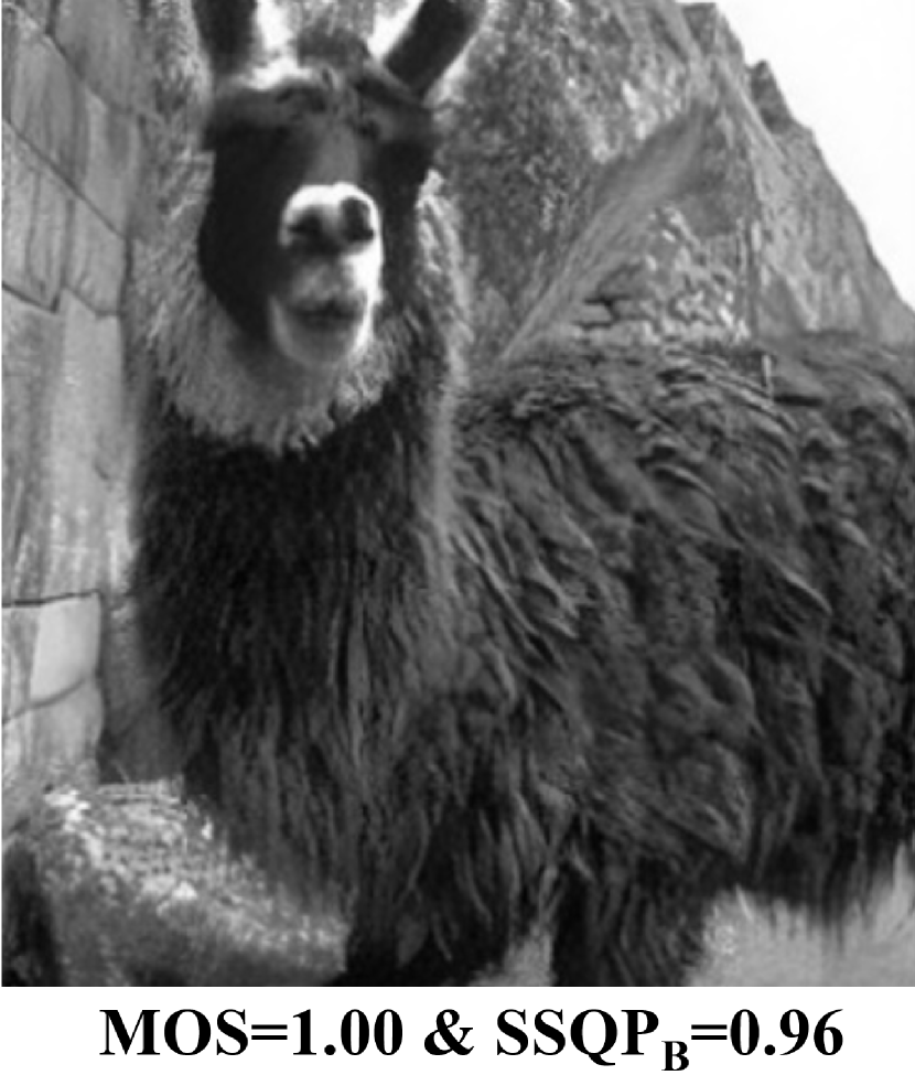
(b)

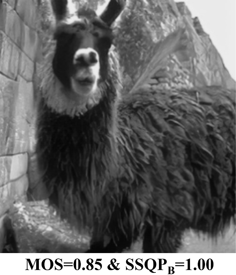
(c)

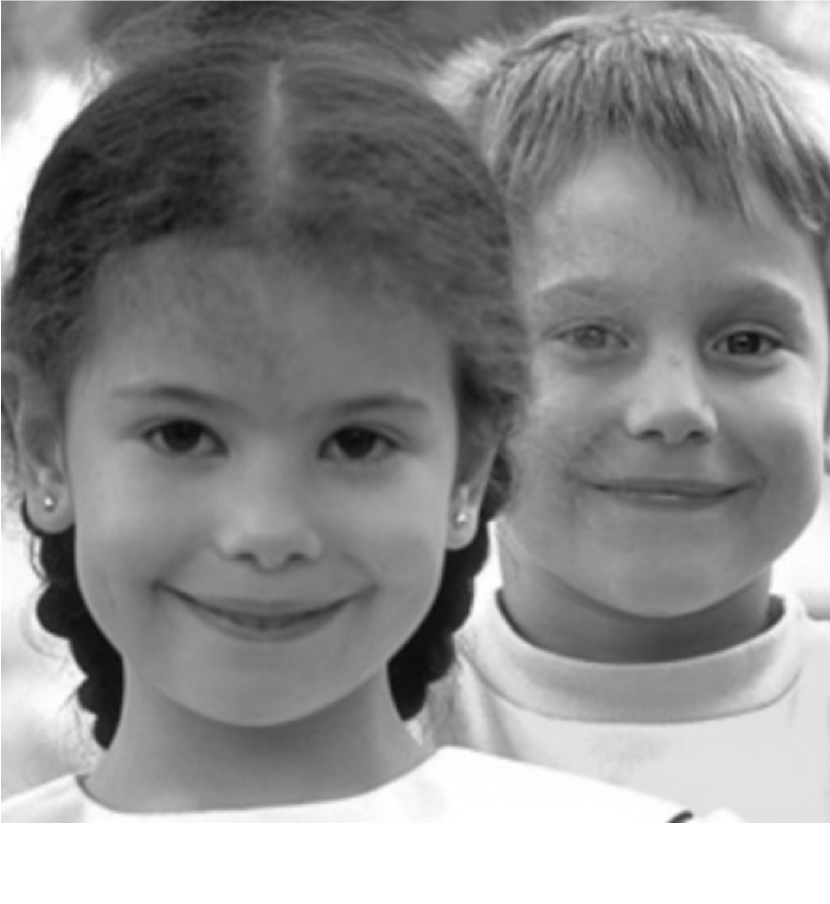
(d)

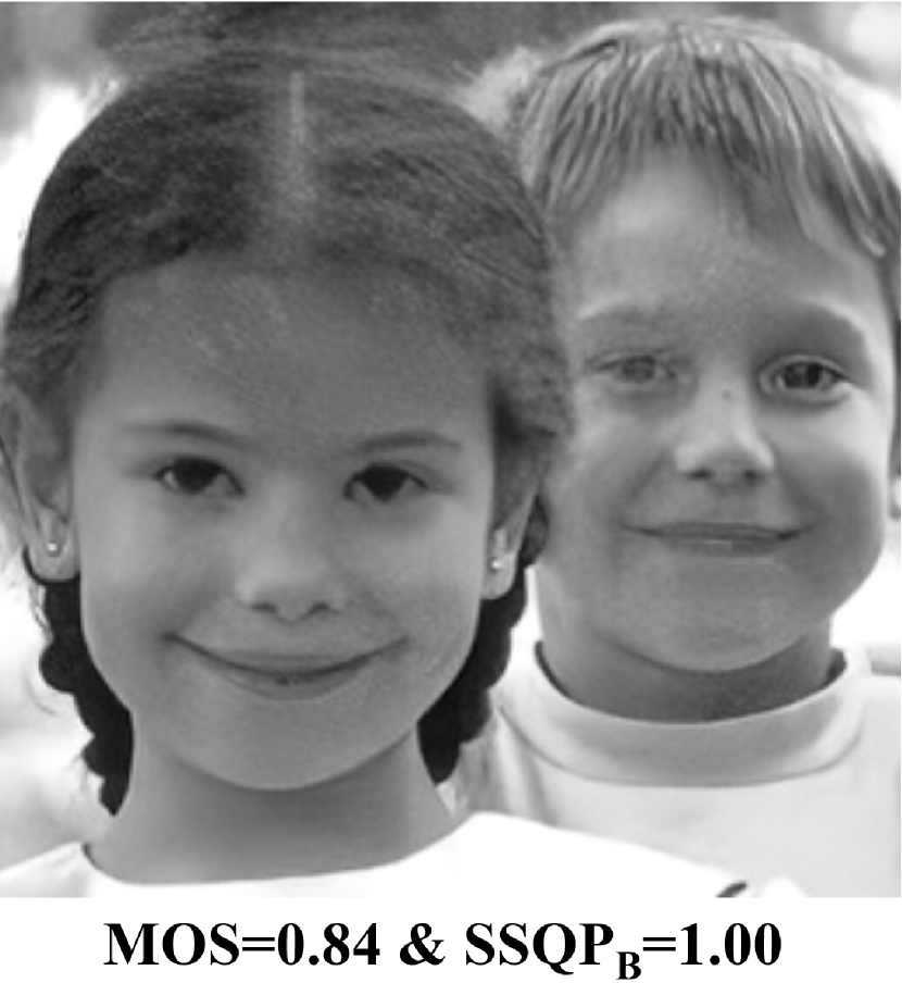
(e)

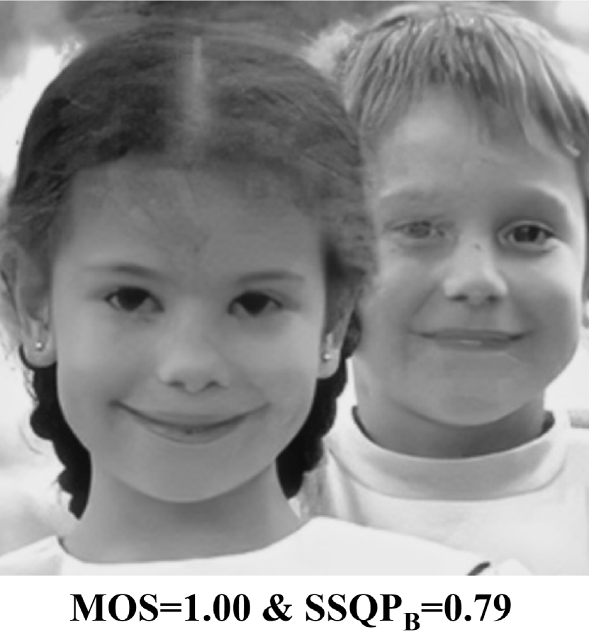
(f)

Figure 11: The examples of the mismatch between MOS and $SSQP_{B}$ for the highest subjective score: (a), (d) the original images, (b), (e) the output images w/ QF20 ($\lambda=0.1$), (c), (f) the output images w/ QF20 ($\lambda=0.01$), where the values of MOS and $SSPQ_{B}$ are scaled from 0 to 1.

In addition, we analyzed those cases where the proposed model fails. Specifically, we calculated the percentages of cases where the worst and the best case MOS and $SSQP_{B}$ matched, as summarized in Table VII. The lowest MOS were mostly observed on JPEG-QF05 images (94%), which $SSQP_{B}$ predicted easily. The highest MOS were distributed among three types of images, but the distributions diverged between MOS and $SSQP_{B}$, as shown in Table VIII, where each entry represents the number of times (of the 18 possible) that the highest MOS or $SSQP_{B}$ prediction occurred. The observed discrepancy is that the majority of highest MOS occurred on images generated using the GAN with $\lambda=0.1$, while the highest $SSQP_{B}$ predictions tended to occur when $\lambda=0.01$. As the value of $\lambda$ increased, the resulting generative images become sharper and more naturalistic, but they also become less natural if $\lambda$ becomes too large. Two examples are given in Fig. 11 (MOS and $SSQP_{B}$ are scaled from 0 to 1). The human subjects preferred the GAN to generate an abundant texture on the llama’s furry parts, while they felt it was unnatural to have excessive texture on people’s faces. Although $SSQP_{B}$ controls the weights between structural/statistical aspects of predicted quality via a multi-stage system, it sometimes fails to precisely determine the proper weights.

V-C Traditional Image Quality Prediction

TABLE IX: Performance comparison on the LIVE image quality database (median PCC, SRCC and RMSE across 1,000 train-test trials for $SSQP_{F}$ and $SSQP_{B}$).

	JP2K			JPEG			WN			GBLUE			FF			ALL
	PCC	SROCC	RMSE	PCC	SROCC	RMSE	PCC	SROCC	RMSE	PCC	SROCC	RMSE	PCC	SROCC	RMSE	PCC	SROCC	RMSE
PSNR	0.90	0.89	7.19	0.86	0.84	8.17	0.99	0.99	2.68	0.78	0.78	9.77	0.89	0.89	7.52	0.82	0.82	9.12
SSIM	0.90	0.93	16.20	0.85	0.90	15.99	0.96	0.96	15.97	0.85	0.89	15.72	0.90	0.94	16.45	0.74	0.85	16.10
MSIM	0.83	0.95	16.20	0.77	0.91	15.99	0.93	0.97	15.97	0.85	0.96	15.72	0.80	0.93	16.45	0.69	0.90	16.10
VSNR	0.95	0.94	4.94	0.94	0.91	5.35	0.98	0.98	3.34	0.93	0.94	5.64	0.90	0.90	7.10	0.89	0.89	7.36
VIF	0.94	0.95	16.20	0.93	0.91	15.99	0.96	0.98	15.97	0.96	0.97	15.72	0.96	0.96	16.45	0.94	0.95	16.10
VIFP	0.93	0.95	16.20	0.91	0.90	15.99	0.96	0.99	15.97	0.94	0.96	15.72	0.95	0.96	16.45	0.92	0.93	16.10
UQI	0.84	0.85	16.20	0.80	0.83	15.99	0.93	0.91	15.97	0.95	0.94	15.72	0.94	0.94	16.45	0.85	0.86	16.10
IFC	0.90	0.89	7.11	0.90	0.86	6.86	0.96	0.94	4.64	0.96	0.96	4.39	0.96	0.96	4.52	0.91	0.91	6.70
NQM	0.94	0.93	5.69	0.93	0.90	5.77	0.99	0.99	2.62	0.88	0.84	7.42	0.84	0.82	9.02	0.87	0.87	7.89
WSNR	0.92	0.91	6.48	0.93	0.89	5.80	0.98	0.97	3.50	0.92	0.91	6.26	0.72	0.76	12.08	0.88	0.88	7.79
SNR	0.87	0.86	8.09	0.85	0.83	8.50	0.97	0.97	3.80	0.76	0.75	10.19	0.89	0.90	7.36	0.81	0.81	9.41
FSIM	0.87	0.96	16.20	0.73	0.91	15.99	0.91	0.97	15.97	0.91	0.97	15.72	0.85	0.95	16.45	0.78	0.92	16.10
GMSD	0.96	0.96	4.36	0.94	0.91	5.25	0.97	0.97	4.16	0.96	0.96	4.34	0.94	0.94	5.63	0.91	0.91	6.73
$SSQP_{F}$	0.95	0.94	4.86	0.94	0.89	5.53	0.99	0.97	2.62	0.96	0.96	4.08	0.96	0.95	4.39	0.95	0.95	4.88
$SSQP_{B}$	0.96	0.95	4.20	0.95	0.91	5.03	0.99	0.98	2.51	0.96	0.95	4.49	0.97	0.95	3.98	0.96	0.95	4.68

We also found that our $SSQP$ IQA model is also capable of predicting traditional perceptual image quality. We compared $SSQP$ against the same benchmark algorithms on the well-known LIVE IQA database [40], It consists of 29 reference images and 982 distorted image with five distortion types: (1) JPEG2000 (JP2K), (2) JPEG, (3) white noise (WN), (4) Gaussian blur (GBLUR), and (5) Fast Fading (FF). For each distorted image, difference mean opinion scores (DMOS) are provided, which is scaled and shifted to the range of [0, 100] where smaller values mean better perceptual quality.
The experimental results are given in Table IX, where the best performing model is boldfaced. For all distortion types, $SSQP$ provided the highest prediction accuracy. These results suggest that GAN quality assessment subsumes some elements of more traditional image quality assessment, and the proposed $SSQP$ model provides more universally robust performance than existing FR metrics.

V-D Perfomance Comparison against DNN-based IQA Models

TABLE X: Performance comparison with two deep learning-based IQA models on the proposed generative image database.

Model	$Subset_{FI}$		$Subset_{PI}$
	PCC	SROCC	PCC	SROCC
DeepQA	0.948	0.918	0.739	0.712
BIECON	0.676	0.865	0.124	0.155
SNPF	0.931	0.877	0.877	0.863
SNPB	0.953	0.891	0.831	0.832

We compared the $SSQP$ against two deep learning based IQA models in [25]. One is $DeepQA$ [24], which is a full-reference model, and the other is $BIECON$ [23] which is a no-reference model. In [25], $DeepQA$ achieved state-of-the-art performance in an FR benchmark comparison, while $BIECON$ also showed top prediction accuracy in the category of no-reference models. The authors provide source codes of both models in the Theano framework, so that we could reproduce the results.
We tested both models on two subsets of our generative image dataset: one is the subset of full-frame images ($subset_{FI}$) and the other is the subset of patch images ($subset_{PI}$) which includes three different type of patches (random/regular/high-level structures). For $BIECON$, following the authors’ instruction, we used SSIM [30] to generate local quality score maps as intermediate targets (see more details in [23]). For $DeepQA$, we trained the network using the patch-based approach adopted in [24] on the $subset_{FI}$, since it consists of two different resolutions and the size of the input images needs to be fixed for training. We used the same patch size of $112$ x $112$ as in [24]. On the single resolution $subset_{PI}$, $DeepQA$ network was trained image-wise. During the experiment, we randomly divided the reference images into two subsets, 80% for training and 20% for testing. The correlation coefficients were averaged after the procedure was repeated 10 times on randomly divided training and testing sets.
The experimental results are given in Table X. On $subset_{FI}$, $SSQP_{B}$ and $DeepQA$ gave comparable performances while $BIECON$’s prediction accuracy was relatively low. On $subset_{PI}$, the performance of $DeepQA$ dropped significantly, while $SSQP_{B}$ still delivered good prediction accuracy. Fig. 10 helps explain this phenomenon. In the case of a full-frame image, even if introduced distortions get stronger, the main structure of the original image could be still maintained (the first column). However, patch images tend to lose their structure as generative distortions get stronger (the second through the fourth columns). $SSQP_{B}$ may cope with this structural collapse by alternatively measuring statistical similarity using the proposed histogram-distance features, as demonstrated in the results of Table IV. CNNs like those used by $DeepQA$ and $BIECON$ have far better abstraction ability than shallow regression methods when representing structures from low-level to high-level. However, they may not capture statistical similarity as well, which plays an important role in assessing the quality of generative images. $BIECON$ failed to provide reliable prediction accuracy.

V-E Cross Database Test

TABLE XI: The database and cross-database tests: performance comparison between $SSQP_{B}$ and $DeepQA$, where the higher value in each pair of corresponding coefficients is marked in boldface.

(a) PCC comparison

$SSQP_{B}$ / $DeepQA$		Dataset for training
		Generative	LIVE	TID2013	CSIQ
Dataset for testing	Generative	0.953 / 0.948	0.671 / 0.829	0.805 / 0.956	0.414 / 0.841
	LIVE	0.900 / 0.898	0.963 / 0.962	0.819 / 0.667	0.881/ 0.890
	TID2013	0.656 / 0.509	0.651 / 0.495	0.872 / 0.884	0.734 / 0.679
	CSIQ	0.828 / 0.819	0.830 / 0.841	0.815 / 0.878	0.888 / 0.962

(b) SRCC comparison

$SSQP_{B}$ / $DeepQA$		Dataset for training
		Generative	LIVE	TID2013	CSIQ
Dataset for testing	Generative	0.891 / 0.918	0.666 / 0.851	0.789 / 0.952	0.417 / 0.876
	LIVE	0.896 / 0.918	0.953 / 0.964	0.810 / 0.556	0.885/ 0.900
	TID2013	0.519 / 0.427	0.532 / 0.430	0.841 / 0.865	0.624 / 0.571
	CSIQ	0.841 / 0.833	0.782 / 0.868	0.749 / 0.889	0.806 / 0.958

To demonstrate the generalization ability of $SSQP$, we conducted a comprehensive set of database and cross-database experiments. First, in addition to the proposed Generative IQA dataset and the LIVE IQA dataset, we added two existing databases: the TID2013 database [65] and the CSIQ database [66]. The TID2013 database consists of 25 reference images and 3,000 distorted images with 24 different distortion types at five levels of degradation, and the MOS of the distorted images is provided. The CSIQ database includes 30 reference images and 866 distorted images of six types: JPEG, JPEG2000, global contrast decrements, AWN, pink gaussian noise and gaussian blur, and it provides DMOS. We compared $SSQP_{B}$ against the DNN-based $DeepQA$ model. On the Generative IQA database, the subset of full-frame images ($subset_{FI}$) was used.
Table XI(b) shows both the database and the cross-database test results. In each pair of corresponding correlation coefficients, we marked the one having higher value in boldface. For the results where training and testing were done on the same databases (the diagonal), $SSQP_{B}$ and $DeepQA$ attained comparable performance. $SSQP_{B}$ provided slightly better performance on the Generative and the LIVE datasets in terms of PCC, whilst $DeepQA$ was advantageous on TID2013 and CSIQ. It is noteworthy that $SSQP_{B}$ was able to provide comparable prediction accuracy as DeepQA, although it has a much smaller number of parameters and a simpler system architecture.
Next, for the cross-database experiments, the model trained on one database was tested on the other database, where the DMOS of the LIVE/CSIQ databases were converted to MOS. For example, when the model is trained on the Generative database and tested on the others, the PCC values were still quite reasonable: 0.900 and 0.828 on LIVE and CSIQ, respectively. The performance drop on TID2013 was due to the fact that it contains many distortion types that do not exist in the Generative database (or arguably, anywhere!) while the number of test images is far larger than in the train database. For the same reason, when we use TID2013 as a train dataset, the trained model delivers PCC values for cross-database tests, close to the results attained when the same database was used for testing as training. It is also noteworthy that although the three existing datasets consist of images of larger resolutions than the Generative dataset, $SSQP$ still achieved reasonable prediction accuracy. It was able to cope with diverse distortion types, which suggests that the structural/statistical features extracted by it reflect general aspects of distortions.

VI Conclusion

We proposed a GAN image quality assessment model called $SSQP$ that was devised using two groups of features representing structural and statistical similarities. We also used a multi-stage parallel boosting system to uncover the nonlinear relationship between the subjective scores and the proposed features. We built a generative image quality database consisting of GAN generative images, and conducted a subjective study on it. The experimental results demonstrate the superiority of $SSQP$ on the new database, outperforming existing FR models by significant margins. Furthermore, it also attained comparable prediction accuracies as recent DNN-based IQA models on three traditional image quality databases.

References

- [1] C. Dong, C. C. Loy, K. He, and X. Tang, “Image super-resolution using deep convolutional networks,” IEEE Transactions on pattern analysis and machine intelligence, vol. 38, no. 2, pp. 295-907, Feb. 2016.
- [2] H, Shin, H. R. Roth, M. Gao, L. Lu, Z. Xu, I. Nogues, J. Yao, D. Mollura, and R. M. Summers, “Deep convolutional neural networks for computer-aided detection: CNN architectures, dataset characteristics and transfer learning,” IEEE Transactions on medical imaging, vol. 35, no. 5, pp. 1285, May. 2016.
- [3] A. Krizhevsky, S. Ilya, and E. H. Geoffrey, “Imagenet classification with deep convolutional neural networks,” Advances in neural information processing systems, pp. 1097-1105. 2012.
- [4] A. Huang and R. Wu, “Deep learning for music,” arXiv preprint , arXiv:1606.04930, 2016.
- [5] L. A. Gatys, A. S. Ecker, and M. Bethge, “Image style transfer using convolutional neural networks,” Proc. IEEE Conf. Comput. Vis. Pattern Recognit. (CVPR), pp. 2414-2423, 2016.
- [6] I. Goodfellow, J. Pouget-Abadie, M. Mirza, B. Xu, D. Warde-Farley, S. Ozair, A. Courville, and Y. Bengio, “Generative adversarial nets.” Advances In Neural Information Processing Systems, pp. 2672-2680. 2014.
- [7] C. Ledig, et al., “Photo-Realistic Single Image Super-Resolution Using a Generative Adversarial Network,” Proc. IEEE Conf. Computer Vis. Pattern Recognition (CVPR), pp. 4681-4690, 2017.
- [8] A. Brock, J. Donahue, and K. Simonyan, ‘’Large scale GAN training for high fidelity natural image synthesis,” Proc. Int’l. Conf. on Learning Representations (ICLR), May, 2019. C. Ledig, et al., “Photo-Realistic Single Image Super-Resolution Using a Generative Adversarial Network,” Proc. IEEE Conf. Computer Vis. Pattern Recognition (CVPR), pp. 4681-4690, 2017.
- [9] E. Agustsson, M. Tschannen, F. Mentzer, R. Timofte, and L. V. Gool, “Generative Adversarial Networks for Extreme Learned Image Compression,” arXiv preprint, arXiv:1804.02958, 2018
- [10] T. Wiegand, G. J. Sullivan, G. Bjontegaard, and A. Luthra, “Overview of the H. 264/AVC video coding standard,” IEEE Transactions on Circuits and Systems for Video Technology, vol. 13, no. 7, pp. 560-576, Jul. 2003.
- [11] G. J. Sullivan, J.-R. Ohm, W.-J. Han, and T. Wiegand, “Overview of the high efficiency video coding (HEVC) standard,” IEEE Transactions on Circuits and Systems for Video Technology, vol. 22, no. 12, pp. 1649-1668, Dec. 2012.
- [12] S. Kim, J. S. Park, C. G. Bampis, J. Lee, M. K. Markey, A. G. Dimakis, and A. C. Bovik, “Adversarial Video Compression Guided by Soft Edge Detection,” arXiv preprint, arXiv:1811.10673, 2018.
- [13] H. R. Sheikh, M. F. Sabir and A. C. Bovik, “A statistical evaluation of recent full reference image quality assessment algorithms,” IEEE Transactions on Image Processing, vol. 15, no. 11, pp. 3440-3451, Nov. 2006.
- [14] A. Moorthy and A. Bovik, “Blind image quality assessment: From natural scene statistics to perceptual quality,” IEEE Transactions on Image Processing, vol. 20, no. 12, pp. 3350-3364, Dec. 2011.
- [15] M. Saad, A. Bovik, and C. Charrier, “Blind image quality assessment: A natural scene statistics approach in the DCT domain,” IEEE Transactions on Image Processing, vol. 21, no. 8, pp. 3339-3352, Aug. 2012.
- [16] A. Mittal, R. Soundararajan, and A. Bovik, “Making a ‘completely blind’ image quality analyzer,” IEEE Signal Process. Lett., vol. 20, no. 3, pp. 209-212, Mar. 2013.
- [17] C. Li, A. Bovik, and X. Wu, “Blind image quality assessment using a general regression neural network,” IEEE Trans. Neural Netw., vol. 22, no. 5, pp. 793-799, May. 2011.
- [18] T. J. Liu, W. Lin, and C. C. J. Kuo, “Image quality assessment using multi-method fusion,” IEEE Transactions on Image Processing, vol. 22, no. 5, pp. 1793-1807, 2013.
- [19] H. Ko, R. Song, and C. C. J, Kuo, “A ParaBoost Stereoscopic Image Quality Assessment (PBSIQA) System,” Journal of Visual Commmication & Image Representation, vol. 45, pp. 156-169, 2017.
- [20] L. He, D. Tao, X. Li, and X. Gao, “Sparse representation for blind image quality assessment,” in Proc. IEEE Conf. Comput. Vis. Pattern Recognit. (CVPR), pp. 1146-1153, Jun. 2012.
- [21] Y. Li et al., “No-reference image quality assessment with shearlet transform and deep neural networks,” Neurocomputing, vol. 154, pp. 94-109, 2015.
- [22] D. Ghadiyaram and A. C. Bovik, “Perceptual Quality Prediction on Authentically Distorted Images Using a Bag of Features Approach,” Journal of Vision, vol. 17, no. 1, pp.32-32, 2017.
- [23] J. Kim and S. Lee, “Fully Deep Blind Image Quality Predictor,” IEEE Journal of Selected Topics in Signal Processing, vol. 11, pp. 206-220, Feb. 2017.
- [24] J. Kim and S. Lee, “Deep Learning of Human Visual Sensitivity in Image Quality Assessment Framework,” Proc. IEEE Conf. Comput. Vis. Pattern Recognit. (CVPR), pp. 1969-1977, Jul. 2017.
- [25] J. Kim, H. Zeng, D. Ghadiyaram, S. Lee, L. Zhang, and A.C. Bovik, “Deep convolutional neural models for picture quality prediction: Challenges and solutions to data-driven image quality assessment,” IEEE Signal Processing Magazine, vol. 34, no. 6, pp. 130-141, Nov. 2017.
- [26] J. Ballé, V. Laparra, and E. P. Simoncelli, “End-to-end Optimized Image Compression,” Proc. Int’l. Conf. on Learning Representations (ICLR2017), Apr. 2017.
- [27] M. Li, W. Zuo, S. Gu, D. Zhao, and D. Zhang, “Learning Convolutional Networks for Content-Weighted Image Compression,” Proc. IEEE Conf. Comput. Vis. Pattern Recognit. (CVPR), pp. 3214-3223, Jun. 2018.
- [28] F. Mentzer, E. Agustsson, M. Tschannen, R. Timofte, and L. V. Gool, “Conditional Probability Models for Deep Image Compression,” Proc. IEEE Conf. Comput. Vis. Pattern Recognit. (CVPR), vol. 1, no. 2, pp. 3, Jun. 2018.
- [29] D. Minnen, J. Balle, and G. D. Toderici, “Joint Autoregressive and Hierarchical Priors for Learned Image Compression,” Proc. 32nd Conference on Neural Information Processing Systems (NIPS), pp. 10794-10803, 2018.
- [30] Z. Wang, A. C. Bovik, H. R. Sheikh and E. P. Simoncelli, “Image quality assessment: From error visibility to structural similarity,” IEEE Transactions on Image Processing, vol. 13, no. 4, pp. 600-612, Apr. 2004.
- [31] Z. Wang, E. P. Simoncelli and A. C. Bovik, “Multi-scale Structural Similarity for Image Quality Assessment,” Proc. 37th IEEE Asilomar Conference on Signals, Systems and Computers, Vol. 2, pp. 1398-1402, Nov. 2003
- [32] O. Rippel and L. Bourdev, “Real-time adaptive image compression,” Proc. 34th International Conference on Machine Learning, vol. 70, pp. 2922-2930, Aug. 2017.
- [33] S. Santurkar, D. Budden, and N. Shavi, “Generative compression,” Proc. Picture Coding Symposium (PCS), pp. 258-262, Jul. 2018.
- [34] L. Galteri, L. Seidenari, M. Bertini, and A. D. Bimbo, “Deep generative adversarial compression artifact removal,” Proc. IEEE Int’l Conf. Comput. Vis. Pattern Recognit. (CVPR), pp. 4826-4835, Apr. 2017.
- [35] J. Oh, X. Guo, H. Lee, R. L. Lewis, and S. Singh, “Action-conditional video prediction using deep networks in atari games,” Advances In Neural Information Processing Systems, pp. 2863-2871, 2015.
- [36] C. Vondrick, H. Pirsiavash, and A. Torralba, “Generating videos with scene dynamics,” Advances In Neural Information Processing Systems, pp. 613-621, 2016.
- [37] M. Ranzato, A. Szlam, J. Bruna, M. Mathieu, R. Collobert, and S. Chopra, “Video (language) modeling: a baseline for generative models of natural videos,” arXiv preprint, arXiv:1412.6604, 2014.
- [38] C. Finn, I. Goodfellow, and S. Levine, “Unsupervised learning for physical interaction through video prediction,” Neural Info Process Syst., pp. 64-72, 2016.
- [39] Z. Liu, R. A. Yeh, X. Tang, Y. Liu, and A. Agarwala, “Video frame synthesis using deep voxel flow,” Proc. IEEE Int’l Conf. Comput. Vis. Pattern Recognit. (CVPR), pp. 4473-4481, Apr. 2017.
- [40] H. R. Sheikh and A. C. Bovik, “Image information and visual quality,” IEEE Transactions on Image Processing, vol. 15, no. 2, pp. 430-444, Feb. 2006.
- [41] A. Mittal, A. K. Moorthy, and A. C. Bovik, “No-reference image quality assessment in the spatial domain,” IEEE Transactions on Image Processing, vol. 21, no. 12, pp. 4695-4708, Dec. 2012.
- [42] J. Guo and H, Chao, “One-to-many network for visually pleasing compression artifacts reduction,” Proc. IEEE Int’l Conf. Comput. Vis. Pattern Recognit. (CVPR), pp. 4867-4876, Apr. 2017.
- [43] K. Simonyan and A. Zisserman, “Very deep convolutional networks for large-scale image recognition,” arXiv preprint, arXiv:1409.1556, 2014.
- [44] T. Y. Lin, M. Maire, S. Belongie, J. Hays, P. Perona, D. Ramanan, P. Dollár and C. L. Zitnick, ‘’Microsoft coco: Common objects in context,” European conference on computer vision, pp. 740-755, Sep. 2014
- [45] P. Arbelaez, M. Maire, C. Fowlkes, and J. Malik, “Contour detection and hierarchical image segmentation,” IEEE Transactions on Pattern Analysis and Machine Intelligence, vol. 33, no. 5, pp. 898-916, 2011.
- [46] ITU-R, Bt.500-11: Methodology for the Subjective Assessment of the Quality of Television Pictures, Tech. Rep., 2002.
- [47] J. Y. Lin, R. Song, C. H. Wu, T. Liu, H. Wang, and C. C. J. Kuo, “MCL-V: A streaming video quality assessment database,” Journal of Visual Communication and Image Representation, vol. 30, pp. 1-9, 2015.
- [48] R. A. Bradley and M. E. Terry, “Rank analysis of incomplete block designs: I. The method of paired comparisons,” Biometrika, vol. 39, no. 3, pp. 324-345, 1952.
- [49] J. C. Handley, “Comparative analysis of Bradley-Terry and Thurstone-Mosteller paired comparison models for image quality assessment,” PICS, vol. 1, pp. 108-112, Apr. 2001.
- [50] M. Narwaria and W. Lin, “SVD-based quality metric for image and video using machine learning,” IEEE Transactions on Systems, Man, and Cybernetics, Part B (Cybernetics), vol. 42, no. 2, pp. 347-364, 2012.
- [51] A. Eskicioglu, A. Gusev, and A. Shnayderman, “An SVD-based grayscale image quality measure for local and global assessment,” IEEE Transactions on Image Processing, vol. 15, no. 2, pp. 422-429, Feb. 2006.
- [52] J. Liu, X. Liu, and X. Ma, “First order perturbation analysis of singular vectors in singular value decomposition,” IEEE Transactions on Signal Processing, vol. 56, no. 7, pp. 3044-3049, Jul. 2008.
- [53] B. Scholkopf and A. J. Smola, “Learning with Kernels: Support Vector Machines, Regularization, Optimization and Beyond,” The MIT Press, 2002.
- [54] D. Basak, S. Pal, and D. C. Patranabis, “Support vector regression,” Neural Inf. Process.-Lett. Rev, vol. 11, no. 10, pp. 203-224, 2007.
- [55] C. W. Hsu, C. C. Chang, and C. J. Lin, “A Practical Guide to Support Vector Classification,” Dept. Comput.Sci., National Taiwan Univ, pp. 1-16, 2003.
- [56] P.1401, “Statistical Analysis, Evaluation and Reporting Guidelines of Quality Measurements,” ITU-T Tech. Rep., 2012.
- [57] VQEG, “Final report from the video quality experts group on the validation of objective models of video quality assessment, phase i,” document com 9-80-e, 2004.
- [58] D. M. Chandler and S. S. Hemami, “VSNR: A wavelet-based visual signal-to-noise-ratio for natural images,” IEEE Transactions on Image Processing, vol. 16, pp.2284-2298, 2007.
- [59] H. R. Sheikh and A. C. Bovik, “A visual information fidelity approach to video quality assessment,” Proc. First International Workshop on Video Processing and Quality Metrics for Consumer Electronics, pp. 23-25. 2005.
- [60] Z. Wang and A. C. Bovik, “A universal image quality index,” IEEE signal processing letters, vol.9, no.3, pp. 81-84, 2002.
- [61] H. R. Sheikh, A. C. Bovik and G. de Veciana, “An information fidelity criterion for image quality assessment using natural scene statistics,” IEEE Transactions on Image Processing, vol.14, no.12, pp. 2117- 2128, Dec. 2005.
- [62] N. Damera-Venkata, T. D. Kite, W. S. Geisler, B. L. Evans, and A. C. Bovik, “Image quality assessment based on degradation model,” IEEE Transactions on Image Processing, vol. 9, no. 4, pp.636-650, 2000.
- [63] L. Zhang, L. Zhang, X. Mou, and D. Zhang, “FSIM: A feature similarity index for image quality assessment,” IEEE Transactions on Image Processing, vol. 20, no. 8, pp. 2378-2386, 2011.
- [64] W. Xue, L. Zhang, X. Mou, and A. C. Bovik, “Gradient magnitude similarity deviation: A highly efficient perceptual image quality index,” IEEE Transactions on Image Processing, vol. 23, no. 2, pp. 684-695, 2014.
- [65] N. Ponomarenko, L. Jin, O. Ieremeiev, V. Lukin, K. Egiazarian, J. Astola, B. Vozel, K. Chehdi, M. Carli, F. Battisti, and C.-C. Jay Kuo, “Image database TID2013: Peculiarities, results and perspectives,” Signal Processing: Image Communication, vol. 30, pp. 57-77, Jan. 2015.
- [66] E. C. Larson and D. M. Chandler, ”Most apparent distortion: Full-reference image quality assessment and the role of strategy,” J. Electron. Imaging, vol. 19, no. 1, pp. 19-19–21, Jan. 2010.