The problem of constructing maximal equiangular tight frames or SICs was raised by Zauner in 1998. Four years ago it was realized that the problem is closely connected to a major open problem in number theory. We discuss why such a connection was perhaps to be expected, and give a simplified sketch of some developments that have taken place in the past four years. The aim, so far unfulfilled, is to prove existence of SICs in an infinite sequence of dimensions.

1. What’s in a name?

We will be concerned with configurations of vectors known as SICs, and pronounced ‘seeks’ because a proof of their existence in all finite dimensions is being sought [1]. The problem is easy to state, but soon reveals unexpected depths. A little more generally we want to find sets of $N$ unit vectors in the finite dimensional Hilbert space ${\bf C}^{d}$, and constants $c_{1}$ and $c_{2}$, such that

$$\sum_{i=1}^{N}|\psi_{i}\rangle\langle\psi_{i}|=c_{1}{\bf 1}$$ (1)

$$|\langle\psi_{i}|\psi_{j}\rangle|^{2}=c_{2}\hskip 14.22636pt\mbox{if}\hskip 14.22636pti\neq j\ .$$ (2)

Such sets are called equiangular tight frames [2]. They can be thought of as $N$ equidistant points in complex projective space, or as a regular simplex in the space containing the convex set of all mixed quantum states, carefully centred and arranged so that all its corners are pure. One proves easily that if the arrangement can be done at all then

$$d\leq N\leq d^{2}\ ,\hskip 28.45274ptc_{1}=\frac{N}{d}\ ,\hskip 28.45274ptc_{2}=\frac{N-d}{d(N-1)}\ .$$ (3)

Existence is not a foregone conclusion. If $d=3$ the possible values of $N$ are 3, 4, 6, 7, and 9, while $N=5$ and $N=8$ are impossible [3]. Minimal ETFs are known as orthonormal bases, while maximal ETFs consisting of $d^{2}$ unit vectors are called SICs. At first they were called Maximale Quantendesigns [4]. Finding SICs is of interest in classical signal processing and in quantum information theory. In the latter context the long acronym SIC-POVM is often used, and then the first three letters stand for “symmetric informationally complete” and the last four for “positive operator valued measure” [5]. Fortunately, in some quantum applications there are conceptual reasons to drop the ungainly last set of four letters [6].

SICs have a background in engineering, but they have recently moved into unexplored regions of algebraic number theory. In 2016 it was conjectured that the numbers needed to construct them are the kind of numbers that appear in the first unsolved case of Hilbert’s 12th problem [7, 8]. The hypothesis was supported by some solid evidence [9, 10]. It bears the hall- mark of truth, because over the last four years it has led to explanations, and predictions, of a very large number of bewildering facts about SICs in various dimensions. Thus the status of the SIC existence problem has changed. There always were good reasons to seek them [11], but now they also seem to be intimately connected to a grand unsolved problem in number theory. In the spirit of the Växjö meetings [12] we hope to provide at least some explanations of this development here: Of the way that the connection to number theory arises (Section 2), of the finite groups that generate SICs and their symmetries (Section 3), and of how the theory as developed so far organizes Hilbert spaces of different dimensions into sequences (Section 4). To keep the discussion simple we will restrict the technical part to the case of odd dimensions only. We do this with some regret because, like the rotation group [13], the groups that generate SICs treat even dimensions in a subtle but ultimately very satisfying way.

There is a school of thought maintaining that SICs will ultimately prove to be as important [1, 14, 15] for quantum foundations as are the orthonormal bases [16]. We do not pursue this argument here, but we do hope to convince the reader that SICs deserve to be spelt with capital letters.

2. Smelling the problem

Why are SICs so hard to find, and why are they connected to number theory? To see this we begin with the famous problem of dividing a circle into $n$ equal parts. We choose $n=7$ as our example. Some group theory clearly enters the problem. What we need are the seven corners of a regular heptagon inscribed in the circle, and we observe that these corners are the orbit of an abelian and cyclic group, $C_{7}$. On closer inspection we realize that the heptagon is left invariant by a larger dihedral group, which is conveniently thought of as a subgroup of the rotation group $SO(3)$. Let us choose one corner to sit at $(x,y)=(1,0)$. As it turns out, placing the remaining six corners leads us to perform some complicated root extractions in order to find their coordinates $x$ and $y$. See the illustration in Figure 1.

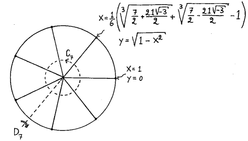
Figure 1: The construction of a regular heptagon involves both group theory and number theory. Incidentally, the fact that cube roots appear in the numbers means that the heptagon cannot be constructed with ruler and compasses.

If we view the plane as a complex plane the position of the corner in the Figure 1 is given by the complex number $\omega=x+iy$. It must be a seventh root of unity, so that $\omega^{7}=1$. It follows that the coordinates of the six corners that we need to construct are the six roots of the polynomial

$$p(z)=z^{6}+z^{5}+z^{4}+z^{3}+z^{2}+z+1\ .$$ (4)

There must be something special about our polynomial, because the roots of a generic polynomial of degree higher than four cannot be given by root extractions at all. This point was explained by Galois, who considered the group that permutes the roots of a given polynomial equation. In our case this group is easily identified. Suppose we consider the permutation that takes $\omega$ to $\omega^{3}$. For consistency we can then deduce that

$$\omega\rightarrow\omega^{3}\rightarrow\omega^{9}=\omega^{2}\rightarrow\omega^{6}\rightarrow\omega^{18}=\omega^{4}\rightarrow\omega^{12}=\omega^{5}\rightarrow\omega^{15}=\omega\ .$$ (5)

We have gone through all the roots! It follows that the Galois group of the polynomial is the abelian group $C_{6}$, and Galois proved that roots of polynomials having an abelian Galois group can always be given in terms of root extractions [17].

Root extraction is a complicated affair, but a beautiful and extremely important feature is waiting in the wings. Introduce the transcendental function

$$e(x)=e^{2\pi ix}\ .$$ (6)

We get the seven corners of our heptagon by evaluating this function at seven rational points. And we see that the trigonometric and exponential functions—discoveries without which our modern civilization would be unthinkable—appear naturally out of the regular polygon problem.

When the problem of the regular $n$-gon is viewed with the eyes of number theory, the key role is played by the cyclotomic or circle-dividing number field with conductor $n$. We obtain this number field by adding an $n$th root of unity to the set of rational numbers and then applying addition and multiplication in every possible way to this set, keeping in mind that $\omega_{n}$ solves an equation analogous to that of setting the polynomial (4) to zero. In this way we take the step from ${\bf Q}$ to ${\bf Q}(\omega_{n})$. The extended number field can be described as a vector space over ${\bf Q}$. For $n=7$ this vector space has 6 dimensions, because any number in ${\bf Q}(\omega_{7})$ is a linear combination of the basis vectors $1,\omega,\dots,\omega^{5}$. The dimension of the vector space is also known as the degree of the number field.

Kronecker and Weber proved that every abelian extension of the rational field, that is to say every extension whose Galois group over the rationals is an abelian group, is a subfield of a cyclotomic field with some conductor $n$. Given that we have an elegant description of the generators of all the cyclotomic fields in terms of a transcendental function evaluated at rational points, this is very satisfactory. A generator of the cyclotomic field with conductor $n$ is obtained as $e(1/n)=e^{2\pi i/n}$. We use the notation $\omega_{n}=e^{2\pi i/n}$ from now on.

Then Kronecker had a dream. Start with the degree 2 number field obtained by adding the square root of an integer $D$ to ${\bf Q}$, and consider the most general abelian extension of that number field. The Galois group of this field considered as an extension of ${\bf Q}$ need not be abelian, but it will enjoy a normal series of the form $e\triangleleft H\triangleleft G$, where $H$ is the Galois group of ${\bf Q}(\sqrt{D})$ over ${\bf Q}$. The notation means that $H$ is a normal subgroup of $G$ and that the group $G/H$ is abelian. Hence the Galois group is close to abelian, and again Galois assures us that the numbers that occur can be arrived at from the rationals by root extractions. Kronecker saw, as in a vision, that if the quadratic base field we start out with uses a negative integer $D$, then it should be possible to complete the story to find special ray class fields housing every abelian extension of this base field, and moreover it should be possible to find transcendental functions (elliptic and modular, in this case) such that the generators of the ray class fields are obtained by evaluating the functions at special points on special elliptic curves.

The program was not quite completed by the time Hilbert posed his famous problems for the twentieth century, but it was soon after [18]. Hilbert was impressed. In his 12th problem he asked for a similar description of the most general abelian extension of an arbitrary base field [19]. Mathematicians soon set to work on this, wisely concentrating on the simplest open case, that of real quadratic base fields ${\bf Q}(\sqrt{D})$ with $D>0$. The twentieth century proved too short for the task. Still a classification of the relevant ray class fields was achieved. They are specified by two positive integers, $D$ that gives the base field and $d$ which gives the conductor. Algorithms for finding generators of these ray class fields have been implemented in computer algebra packages. But the problem of writing down explicit generators for them, preferably by starting from some transcendental function, remains open. As the example of the heptagon shows, a solution may have far-reaching consequences.

Now we come to the point. The Ray Class Hypothesis states that the numbers needed to construct a SIC in dimension $d>3$ generate a ray class field over a real quadratic base field [7, 8]. The conductor of the field is equal to $d$ if $d$ is odd and $2d$ if $d$ is even, while the integer $D$ that determines the base field is given by [20]

$$D=(d+1)(d-3)\ .$$ (7)

We will return to this interesting formula in Section 4. It does make it appear as if the SICs may be the geometrical objects that hold the key to a part of Hilbert’s 12th problem.

There is a complication here, which is that in almost all of the dimensions that have been investigated several unitarily inequivalent SICs do exist [9, 22]. Then the hypothesis says that at least one of them can be constructed using the ray class field. If one of the SICs is singled out as having the highest symmetry, this is it [10]. The other SICs require further abelian extensions of the ray class field.

As a preparation for Section 3 we notice the fact that for the special choice of conductors implied by the formula the ray class field will contain the cyclotomic field ${\bf Q}(\omega_{2d})$ as a subfield [7]. We also note that if $d$ is odd then $-\omega_{d}$ is a $2d$th root of unity, and it certainly belongs to ${\bf Q}(\omega_{d})$. Thus ${\bf Q}(\omega_{d})={\bf Q}(\omega_{2d})$ when $d$ is odd, but not when $d$ is even. As a preparation for Section 4 we observe that if we fix the base field and consider two different conductors $d_{1}$ and $d_{2}$ then, by the very definition of conductors, the ray class field with conductor $d_{1}$ is a subfield of that with conductor $d_{2}$ if and only if $d_{1}$ is a divisor of $d_{2}$. The reader may easily check this for the special case of cyclotomic fields.

3. The acting groups

To find SICs we first ask if they are orbits of a group, as the $n$-gons are. Gerhard Zauner, and independently Joseph Renes and his coworkers, conjectured that a discrete Heisenberg group plays this role [4, 5]. This group is a central extension of the product of two cyclic groups $C_{d}\times C_{d}$, and its unitary representation is essentially unique. Its unitary automorphism group, from which extra symmetries of the SICs are taken, contains as a factor group the discrete symplectic group acting on the discrete ‘plane’ of the group elements. Zauner made a further mysterious conjecture, later sharpened [21] to say that every SIC has an extra symmetry of order 3. Closer examination led to more detailed conjectures about higher symmetries appearing in special cases in special dimensions [9, 22, 23].

Numerical searches for SICs are made easier once it is assumed that they are orbits under a group. It is then enough to find a single fiducial vector from which the group creates the SIC. In this way SICs have been found numerically in all dimension $d\leq 193$ and in some higher dimensions, the record being $d=2208$ [22, 24]. In his thesis Zauner also provided exact solutions in dimensions 4 and 5. (Dimension 2 is trivial. A solution in dimension 3, related to an elliptic curve invariant under this very group, was provided by Hesse in 1844 [25].) By now more than one hundred exact solutions are known [9, 10, 24].

Heisenberg groups are important throughout quantum mechanics and signal processing alike. For us a convenient starting point is the book by Weyl [26]. The Weyl–Heisenberg group is generated by $X,Z,\omega$, subject to the relations

$$ZX=\omega XZ\ ,\hskip 14.22636pt\omega X=X\omega\ ,\hskip 14.22636pt\omega Z=\omega Z\ ,\hskip 14.22636ptX^{d}=Z^{d}=\omega^{d}={\bf 1}\ .$$ (8)

There is one such group for each choice of the integer $d$. Weyl thought of them as toy models of the group that encapsulates the non-commutativity of position and momentum, which at some point became known as the Heisenberg group. The discrete group has an essentially unique irreducible unitary representations in a Hilbert space of dimension $d$. We first fix $\omega$ to be

$$\omega=\omega_{d}=e^{\frac{2i\pi}{d}}$$ (9)

(times the unit matrix, which is understood). Actually any primitive $d$th root of unity would do, which is why the representation is only ‘essentially’ unique. In the basis where $Z$ is chosen to be diagonal it is

$$Z|i\rangle=\omega^{i}|i\rangle\ ,\hskip 22.76219ptX|i\rangle=|i+1\rangle\ ,$$ (10)

where the basis vectors are labelled by integers counted modulo $d$.

The representation makes use only of numbers from the cyclotomic field ${\bf Q}(\omega_{d})$. But if the dimension $d$ is odd then ${\bf Q}(\omega_{d})={\bf Q}(\omega_{2d})$. To save the one-to-one correspondence between dimensions and cyclotomic fields one can extend the centre of the group to include $2d$th roots of unity if $d$ is even. There are actually several good reasons for this move [7, 21], but as advertized in the introduction we will restrict the discussion to the case of odd $d$ from now on in order to keep the story brief.

To understand how the Weyl–Heisenberg group depends on the dimension $d$ we begin by recalling an interesting fact about cyclic groups. It is easy to see that $C_{4}\neq C_{2}\times C_{2}$, because every element of the product group squares to the identity, while $C_{4}$ contains elements of order 4. On the other hand it is easy to convince oneself that $C_{6}=C_{2}\times C_{3}$. What makes this case different is that 2 and 3 are relatively prime, that is to say their greatest common divisor equals 1. Here it means that the cyclic groups, and indeed the Weyl–Heisenberg groups, can be broken down into relatively prime atoms. That is to say, if $H(d)$ denotes the group in dimension $d$, and if $d$ can be decomposed into primes as

$$d=p_{1}^{n_{1}}\cdot p_{2}^{n_{2}}\cdot\dots\cdot p_{r}^{n_{r}}\$$ (11)

then

$$H(d)=H(p_{1}^{n_{1}})\times H(p_{2}^{n_{2}})\times\dots\times H(p_{r}^{n_{r}})\ .$$ (12)

To prove this one applies the Chinese remainder theorem from elementary number theory [27]. So it suffices to understand the group in prime power dimensions. We remark that if the dimension is prime then it can be proved that every SIC that is generated by a group is generated by the Weyl–Heisenberg group [28].

The central extension, with its troublesome phase factors, is there only to provide an interesting representation theory. When the group acts on projective space it does so as the product of two cyclic groups, so it makes sense to select a set of only $d^{2}$ group elements to work with. Nevertheless it pays to pay careful attention to the phase factors when we do so. We define the displacement operators [21]

$$D_{i,j}=\tau^{ij}X^{i}Z^{j}\ \ ,\hskip 22.76219pt\tau=-e^{\frac{\pi i}{d}}\ .$$ (13)

Notice that $\tau$ is a $d$th root of unity when $d$ is odd, as we assumed it to be for simplicity. A key fact about the displacement operators is that they form a unitary operator basis, which is why Schwinger allowed the Weyl–Heisenberg group to take the centre stage in his presentation of quantum mechanics [29]. The group law takes the form

$$D_{i,j}D_{k,l}=\tau^{ki-lj}D_{i+k,j+l}\hskip 14.22636pt\Leftrightarrow\hskip 14.22636ptD_{\bf p}D_{\bf q}=\tau^{<{\bf p},{\bf q}>}D_{{\bf p}+{\bf q}}\ .$$ (14)

Here we introduced two-component ‘vectors’ ${\bf p},{\bf q}$ whose components are integers modulo $d$, as well as the symplectic form $<{\bf p},{\bf q}>$. The latter is very useful when we consider the unitary automorphism group, that is to say the group of unitary operators that permute the elements of the Weyl–Heisenberg group under conjugation. It is known as the Clifford group [30], and contains the symplectic group $SL(2,{\bf Z}_{d})$ as a factor group. The latter has a defining representation in terms of two-by-matrices $F$ obeying

$$<F{\bf p},F{\bf q}>\ =\ <{\bf p},{\bf q}>\ {\rm modulo}\ d\ .$$ (15)

These are precisely the matrices having unit determinant and entries that are integers modulo $d$. Once the representation of the Weyl–Heisenberg has been chosen the unitary representative $U_{F}$ of the symplectic matrix $F$ is completely fixed up to phase factors [21] by the defining relation

$$U_{F}D_{\bf p}U_{F}^{-1}=D_{F{\bf p}}\ .$$ (16)

Here we want to stress that the entire Clifford group is represented by matrices all of whose entries lie in the cyclotomic number field. Acting on any vector whose components are built using a number field that includes the cyclotomic field, it will produce new vectors built from the same kind of numbers. This is clearly relevant for us.

The Chinese remainder theorem again makes itself felt at this point, so that the Clifford group splits into a direct product determined by the decomposition of the dimension into prime factors: it is enough to understand how it behaves in prime power dimensions. For $d=3,5$ the symplectic groups enjoy the group isomorphisms

$$SL(2,{\bf Z}_{3})/\pm{\bf 1}={\bf T}\ \$$ (17)

$$SL(2,{\bf Z}_{5})/\pm{\bf 1}={\bf I}\ ,$$ (18)

where ${\bf T}$ and ${\bf I}$ are the symmetry groups of the tetrahedron and the dodecahedron (or icosahedron), respectively. A reader equipped with cardboard models of these polyhedra can therefore take in the structure of these groups at a glance. But some structure is hidden since we have divided out the centre of the symplectic group. It consists of an order two matrix with a simple unitary representative,

$$F=-{\bf 1}\hskip 14.22636pt\Rightarrow\hskip 14.22636pt\langle i|U_{F}|j\rangle=\delta_{0,i+j}\ .$$ (19)

We denote this particular unitary operator $U_{F}$ either as $U_{P}$ or as $A_{\bf 0}$. It is known as the parity operator. We can use it to construct an alternative unitary and Hermitean operator basis, consisting of the phase point operators [31]

$$A_{\bf p}=D_{\bf p}A_{\bf 0}D_{\bf p}^{-1}\ .$$ (20)

This operator basis is significant in the SIC problem in more ways than one. One can show that the spectrum of a phase point operator consists of $(d+1)/2$ eigenvalues $+1$, and $(d-1)/2$ eigenvalues $-1$. (Our self-imposed restriction to odd $d$ is still in force.) It follows that the phase point operators give us a set of $d^{2}$ subspaces of dimension $(d+1)/2$, defined by the projectors

$$\Pi_{\bf p}=\frac{1}{2}({\bf 1}+A_{\bf p})\ .$$ (21)

We can think of these subspaces as points in the Grassmannian $Gr_{(d+1)/2,d}$, analogously to how we regard one-dimensional subspaces as points in projective space. There is a natural notion of chordal distance $D_{\rm ch}$ between points in a Grassmannian, which if we identify the subspaces with the projectors is given by

$$D_{\rm ch}^{2}(\Pi_{\bf p},\Pi_{\bf q})=\mbox{Tr}(\Pi_{\bf p}-\Pi_{\bf q})^{2}\ .$$ (22)

A quick calculation confirms that the subspaces defined by the operator basis form a set of $d^{2}$ equidistant points in the Grassmannian. Exactly why we bring up this curious point will become clear in Section 4, but it may not be amiss to remark that these subspaces play a role in the theory of elliptic normal curves transforming into themselves under the Weyl–Heisenberg group [32].

4. To build a ladder to the stars

We now return to the key formula (7), to see how different dimensions are connected to each other by the number theoretical properties of the SICs they contain. We rewrite it a little by setting $D=m^{2}D_{0}$, where $m$ is any integer and $D_{0}$ does not have square factors. Clearly ${\bf Q}(\sqrt{D})={\bf Q}(\sqrt{D_{0}})$. The formula becomes

$$(d+1)(d-3)=D=m^{2}D_{0}\ .$$ (23)

It can be read in two directions. If we begin in a Hilbert space of dimension $d$ we use it to determine $D$, and hence the base field needed in the construction of SICs. But we can also fix the square-free part $D_{0}$ and solve the Diophantine equation for $d$ in order to establish, via the SICs, a number theoretical connection between different dimensions. Because the integer $m$ is free the result is an infinite sequence $\{d_{i}\}_{i=1}^{\infty}$ of dimensions known as a dimension tower. The entries of the sequence are given by a simple formula [7, 8] which however we do not give here since this would require a detour to introduce the unit group of the base field [27]. Instead we give the beginnings of two such towers in Figure 2.

Figure 2: The first 10 dimensions connected by $D_{0}=5$ and by $D_{0}=3$. Dimensions for which exact SICs are known [9, 23, 24, 33] are in boldface. A field is a subfield of another if its conductor divides that of the other. In the picture this happens if the other field can be reached by walking along upwards directed links. When $d$ is even the conductor equals $2d$, but this does not affect this ordering. Vertical lines (or ‘ladders’) arise from the substitution $d\rightarrow d(d-2)$.

The Figure encodes information about when an entry $d_{i}$ is a divisor of another entry $d_{j}$. This is important because when one conductor is a divisor of another it implies that the first ray class field is contained in the other. The vertical ladders in Figure 2 are meant to attract attention. They arise from the simple observation that

$$d\rightarrow d(d-2)\hskip 14.22636pt\Rightarrow\hskip 14.22636pt(d+1)(d-3)\rightarrow(d-1)^{2}(d+1)(d-3)\ .$$ (24)

The square free part $D_{0}$, and hence the base field, is unchanged by the substitution. Moreover, since (obviously) $d$ divides $d(d-2)$ the field used in the higher dimension always contains that used in the lower. With our choice of labelling, every odd numbered entry $d_{2n+1}$ in a tower starts its own ladder, while the entries $d_{2^{r}\cdot(2n+1)}$ are said to sit on rung $r$ of some ladder.

It is tempting to believe that some unknown physics is hidden in these sequences. It is also tempting to believe that one can prove SIC existence for all the dimensions in such a sequence in some inductive way. At the moment this is just a dream, but bits and pieces of what looks like an argument to this effect have materialized [34, 35, 36, 37]. We can simplify the story quite a bit by starting it from an observation by Renes et al. [5], and this is what we propose to do here.

Let $|\psi_{0}\rangle$ be a fiducial vector for a SIC in dimension $d$. Form the vector $|\psi_{0}\rangle\otimes|\psi_{0}\rangle$ in the symmetric subspace ${\bf C}^{d(d+1)/2}$ of ${\bf C}^{d^{2}}$. The Weyl–Heisenberg group can be made to act on this vector. Pausing to polish our conventions we define $\omega=e^{2\pi i/d}$ and

$$\left.\begin{array}[]{ccc}{\bf X}&=&X\otimes X\\ {\bf Z}&=&Z^{\frac{d+1}{2}}\otimes Z^{\frac{d+1}{2}}\end{array}\right\}\hskip 14.22636pt\Rightarrow\hskip 14.22636pt{\bf Z}{\bf X}=\omega{\bf X}{\bf Z}\ .$$ (25)

Note that our restriction to odd $d$ is still in force. The case of even $d$ is more interesting [35, 37], but takes more space. We now have the Weyl–Heisenberg group $H(d)$ acting on ${\bf C}^{d^{2}}$, and can define the displacement operators

$$\tilde{D}_{ij}=\tau^{ij}{\bf X}^{i}{\bf Z}^{j}\ .$$ (26)

By assumption

$$\langle\psi_{0}|D_{\bf p}|\psi_{0}\rangle=\left\{\begin{array}[]{ccl}1&\mbox{if}&{\bf p}={\bf 0}\\ \frac{e^{i\theta_{i,j}}}{\sqrt{d+1}}&\mbox{if}&{\bf p}\neq{\bf 0}\ ,\end{array}\right.$$ (27)

where the phase factor is a SIC overlap phase from dimension $d$. Using the definition of $\tilde{D}_{\bf p}$ we see that

$$\langle\psi_{0}|\langle\psi_{0}|\tilde{D}_{\bf p}|\psi_{0}\rangle|\psi_{0}\rangle=\left\{\begin{array}[]{ccl}1&\mbox{if}&{\bf p}={\bf 0}\\ \frac{e^{2i\theta_{i,j^{\prime}}}}{d+1}&\mbox{if}&{\bf p}\neq{\bf 0}\end{array}\right.\ ,\hskip 14.22636ptj^{\prime}=\frac{d+1}{2}j\ .$$ (28)

From the SIC in dimension $d$ we have obtained an ETF consisting of $d^{2}$ vectors in dimension $d(d+1)/2$ [5].

We are representing the Weyl–Heisenberg group $H(d)$ in ${\bf C}^{d^{2}}$, and from Weyl’s book we know that the representation must be reducible [26]. To take advantage of this we introduce the orthonormal basis

$$|ii\rangle=|i\rangle|i\rangle,\hskip 5.69054pt|(i,j)\rangle=\frac{1}{\sqrt{2}}(|i\rangle|j\rangle+|j\rangle|i\rangle),\hskip 5.69054pt|[i,j]\rangle=\frac{1}{\sqrt{2}}(|i\rangle|j\rangle-|j\rangle|i\rangle)\ .$$ (29)

We now forget about the tensor product structure, and introduce a new one. With a suitable ordering of the new basis vectors we can ensure that the representation uses block diagonal matrices $\tilde{D}_{\bf p}$ carrying copies of the dimension $d$ displacement operators $D_{\bf p}$ in the blocks. Hence we can write

$$\tilde{D}_{\bf p}={\bf 1}\otimes D_{\bf p}\ ,$$ (30)

where we let the dimension in which the identity operator acts depend on the context. If we act on ${\bf C}^{nd}$ we need $n$ blocks, and the dimension we need is $n$.

Elementary linear algebra tells us if there exists an ETF with $d^{2}$ vectors in dimension $d(d+1)/2$ then there must exist an ETF with $d^{2}$ vectors in dimension $d(d-1)/2$. To see why we renormalize the vectors by defining

$${\bf u}_{\bf p}=\sqrt{d+1}\tilde{D}_{\bf p}|\psi_{0}\rangle|\psi_{0}\rangle\ .$$ (31)

We let these vectors form the columns of a $d(d+1)/2\times d^{2}$ matrix $M$. From the tight frame condition (1) it follows that the rows of this matrix are orthogonal to each other, $MM^{\dagger}=2d{\bf 1}_{d(d+1)/2}$. We then fill out this rectangular matrix to a unitary matrix

$$U=\frac{1}{\sqrt{2d}}\left[\begin{array}[]{cccc}{\bf u}_{0}&{\bf u}_{1}&\dots&{\bf u}_{d^{2}-1}\\ \hline\cr{\bf v}_{0}&{\bf v}_{1}&\dots&{\bf v}_{d^{2}-1}\end{array}\right]\ ,\hskip 22.76219ptUU^{\dagger}=U^{\dagger}U={\bf 1}_{d^{2}}\ .$$ (32)

This is always possible. From unitarity it follows that

$$({\bf v}_{\bf p},{\bf v}_{\bf p})=\left\{\begin{array}[]{ccl}d-1&\mbox{if}&{\bf p}={\bf 0}\\ -e^{2i\theta_{i,j^{\prime}}}&\mbox{if}&{\bf p}\neq{\bf 0}\ .\end{array}\right.$$ (33)

Finally we renormalize the ${\bf v}_{\bf p}$ to obtain a set of unit vectors in ${\bf C}^{d(d-1)/2}$, and we sneak in the assumption that the columns of $U$ are generated, in their entirety, by acting with $\tilde{D}_{\bf p}$ on the first column. We obtain

$$|\Psi_{\bf p}\rangle=\frac{1}{\sqrt{d-1}}{\bf v}_{\bf p}=\tilde{D}_{\bf p}|\Psi_{0}\rangle\ .$$ (34)

We now have an equiangular tight frame in ${\bf C}^{d(d-1)/2}$,

$$\langle\Psi_{0}|\tilde{D}_{\bf p}|\Psi_{0}\rangle=\left\{\begin{array}[]{ccl}1&\mbox{if}&{\bf p}={\bf 0}\\ -\frac{e^{2i\theta_{i,j^{\prime}}}}{d-1}&\mbox{if}&{\bf p}\neq{\bf 0}\ .\end{array}\right.$$ (35)

This is known as the Naimark complement of the ETF we started out with. We know that it exists, and its Gram matrix is completely known.

A little rewriting will reveal what we are driving at:

$$\langle\Psi_{0}|\tilde{D}_{\bf p}|\Psi_{0}\rangle=-\frac{e^{2i\theta_{i,j^{\prime}}}}{d-1}\hskip 5.69054pt\Leftrightarrow\hskip 5.69054pt\langle\Psi_{0}|{\bf 1}_{\frac{d-1}{2}}\otimes D^{(d)}_{\bf p}|\Psi_{0}\rangle=-\frac{e^{2i\theta_{i,j^{\prime}}}}{\sqrt{d(d-2)+1}}\ .$$ (36)

The displacement operators that occur here are those for dimension $d$, but the absolute value of the right hand side is that appropriate for a SIC in dimension $d(d-2)$, the dimension one rung above the dimension we started out with. The vectors do not sit in that dimension, but we now observe that

$$\frac{d-1}{2}=\frac{d-2+1}{2}\ .$$ (37)

From Section 3 we recall that this is the dimension of the positive parity eigenspace in ${\bf C}^{d-2}$. Hence we can embed the fiducial vector $|\Psi_{0}\rangle$ in that eigenspace to obtain a vector in ${\bf C}^{d-2}\otimes{\bf C}^{d}$, taking care to adjust the basis so that the representation of the parity operator $U_{P}$ becomes the standard one (19). We then have

$$\langle\Psi_{0}|{\bf 1}_{d-2}\otimes D^{(d)}_{\bf p}|\Psi_{0}\rangle=-\frac{e^{2i\theta_{i,j^{\prime}}}}{\sqrt{d(d-2)+1}}\ ,$$ (38)

and the symmetry

$$U_{P}^{(d-2)}\otimes{\bf 1}_{d}|\Psi_{0}\rangle=|\Psi_{0}\rangle\ .$$ (39)

Looking carefully at the Scott–Grassl conjectures [9, 22] we find that they say that a SIC fiducial with this symmetry always exists in dimensions of the form $d(d-2)$, so this looks like a SIC.

It remains to arrange that

$$|\langle\Psi_{0}|D^{(d-2)}_{\bf p}\otimes D^{(d)}_{\bf p}|\Psi_{0}\rangle|^{2}=\frac{1}{d(d-2)+1}\ .$$ (40)

This is the hard part. However, it is at least consistent with our observation (in Section 3) that the Grassmannian of $(d+1)/2$-planes in ${\bf C}^{d}$ contains a Weyl–Heisenberg multiplet of planes at constant mutual chordal distance, see eq. (22). When we change the dimension to $d-2$ and then factor in an extra Hilbert space of dimension $d$, it implies that can create a Weyl–Heisenberg multiplet consisting of $(d-2)^{2}$ equidistant subspaces of dimension $d(d-1)/2$ sitting in ${\bf C}^{d(d-2)}$. Each of them contains an ETF, and the total number of vectors is $d^{2}(d-2)^{2}$, just right for a SIC.

The reader can see that our story exists only in bits and pieces that do not quite hang together. It is being improved [38]. At first it was told backwards [34]. For the 22 cases where numerical solutions were available (or were made available by Andrew Scott) in the higher dimension, it was found that for every SIC in dimension $d$ one of the SICs in dimension $d(d-2)$ is aligned to it in the sense that it has the property described by eq. (38). It was then proved that this property implies the existence of embedded ETFs according to the pattern we just discussed—except that the proof in the even dimensional case was given later [35] due to the complications that we have ignored here. Notice that, given that the aligned higher dimensional SIC fiducial vector contains only $2d(d-2)$ real numbers to be solved for, the number of overlap phases that are known ‘from below’ is quite significant. This observation was used to obtain the solution in $d=323=19\cdot 17$ in exact form [23]. The upshot is that we know 23 instances where squared SIC overlap phases are helpful when we try to climb from one rung to another on some ladder—but we still cannot do it in an effortless manner.

But squared SIC overlap phases also provide a concrete bridge from the SIC problem to the Stark conjectures [39]. The latter were proposed in 1976, and their proofs would constitute a significant advance towards the solution of Hilbert’s 12th. A little bit more precisely: It was shown by Kopp [40] that in some, and conjecturally all, prime dimensions equal to 2 modulo 3 a Galois transformation of the base field turns the squared SIC phases into Stark units. This has now been elucidated somewhat further [41], and provided that the restriction to special choices of $d$ can be removed it seems to add credibility to our program.

Still it may seem that we have been ignoring the harsh realities of number theory. They tell us that the degrees of the ray class fields rise very quickly as we ascend the ladders. Going from eq. (38) to eq. (40) will be difficult. But to get to heaven it is enough to climb one ladder, and it could be that it would be easier to do so on a special one. A candidate is perhaps the ladder starting at $d=5$, because the SIC fiducials appearing on its first three rungs can be written down exactly in a remarkably simple way [33]. Some of the reasons why this works continue to hold throughout the entire $D_{0}=3$ tower, and have to do with the way the dimensions appearing in the sequence decompose into primes once we are above the second rung [42], and with the fact that SIC symmetries are especially transparent in prime dimensions equal to 1 modulo 3 [21]. It also has to do with the ‘decoupling’ phenomenon first observed in dimension $d=323$ [23], according to which that SIC fiducial vector can be constructed using a fairly small subfield of the ray class field, the cyclotomic numbers entering the displacement operators providing the rest.

5. The fifth section

Is it likely that the SIC problem will have a happy end, in the sense that it will prove important for the Foundations of Physics? I think so. The QBist approach to the foundations of quantum mechanics certainly suggests it [1, 14, 15]. The number theoretical angle suggests additional arguments. SICs force us to pay attention to the nature of the numbers that are being used in quantum physics, and this shows that quantum mechanics knows more about discrete structures inside the continuum than one might think [43]. There have been many attempts to build up physical theory from discreteness. It may be more interesting to concentrate on things which, in fact, are discrete in existing theory and try to use them as primary concepts. (Yes, this has been said before [44].) It is also striking to the eye that SICs arrange Hilbert space dimensions into ordered sequences. When the representation theory of Lie groups was worked out for the first time, sequences of dimensions such as $3,8,10,\dots$ must have seemed rather divorced from reality. They are not, as we were taught by the originators of the quark model. Because of the uncertain state that the SIC problem is presently in we must let the matter rest here, but more things may come.

Acknowledgements: I thank my students for collaboration and Andrei Khrennikov for the opportunity to present the SIC problem at the Växjö meetings, where so many interesting discussions about SICs have happened.

References

- [1] C. A. Fuchs and R. Schack, From quantum interference to Bayesian coherence and back round again, in L. Accardi et al. (eds.): Foundations of Probability and Physics - 5, AIP Conf. Proc. 1101, New York 2009.
- [2] S. Waldron: An Introduction to Finite Tight Frames, Basel: Birkhäuser 2018.
- [3] F. Szöllősi, All complex equiangular tight frames in dimension 3, arXiv:1402.6429.
- [4] G. Zauner: Quantendesigns. Grundzüge einer nichtkommutativen Designtheorie, PhD thesis, Universität Wien, 1999; also published as Quantum designs: Foundations of a noncommutative design theory, Int. J. Quant. Inf. 9 (2011) 445.
- [5] J. M. Renes, R. Blume-Kohout, A. J. Scott, and C. M. Caves, Symmetric informationally complete quantum measurements, J. Math. Phys. 45 (2004) 2171.
- [6] A. Tavakoli, M. Farkas, D. Rosset, J.D. Bancal, and J. Kaniewski, Mutually unbiased bases and symmetric informationally complete measurements in Bell experiments: Bell inequalities, device-independent certification and applications, arXiv:1912.03225.
- [7] M. Appleby, S. Flammia, G. McConnell, and J. Yard, Generating ray class fields of real quadratic fields via complex equiangular lines, arXiv:1604.06098, Acta Arithmetica 192 (2020) 211.
- [8] M. Appleby, S. Flammia, G. McConnell, and J. Yard, SICs and algebraic number theory, Found. Phys. 47 (2017) 1042.
- [9] A. J. Scott and M. Grassl, SIC-POVMs: A new computer study, J. Math. Phys. 51 (2010) 042203.
- [10] M. Appleby, T.-Y. Chien, S. Flammia, and S. Waldron, Constructing exact symmetric informationally complete measurements from numerical solutions, J. Phys. A51 (2018) 165302.
- [11] C. A. Fuchs, M. C. Hoang, and B. C. Stacey, The SIC question: History and state of play, Axioms 6 (2017) 21.
- [12] A. Khrennikov and B. C. Stacey, Aims and scope of the special issue, “Quantum foundations: Informational perspective”, Found. Phys. 47 (2017) 1003.
- [13] F. Klein and A. Sommerfeld: Theorie des Kreisels I, Leipzig: Teubner 1897; also published as The Theory of the Top I, Boston: Birkhäuser 2010.
- [14] M. Appleby, C. A. Fuchs, B. C. Stacey, and H. Zhu, Introducing the Qplex: A novel arena for quantum theory, Eur. Phys. J. D71 (2017) 197.
- [15] J. B. DeBrota, C. A. Fuchs, and B. C. Stacey, Symmetric informationally complete measurements identify the irreducible difference between classical and quantum systems, Phys. Rev. Res. 2 (2020) 013074.
- [16] A. M. Gleason, Measures on the closed subspaces of a Hilbert space, J. Math. Mech. 6 (1957) 885.
- [17] I. Stewart: Galois Theory, Chapman and Hall, London 1973.
- [18] N. Schappacher, On the history of Hilbert’s 12th problem. A comedy of errors, Matériaux pour l’historie des mathématiques au XXe siècle (Nice 1996), p. 243, Séminaires et Congres 3, Paris 1998.
- [19] D. Hilbert, Matematische Probleme, Göttinger Nachrichten (1900) 253; also published as Mathematical problems, Bull. AMS 8 (1902) 437.
- [20] D. M. Appleby, H. Yadsan-Appleby, and G. Zauner, Galois automorphisms of symmetric measurements, Quantum Inf. Comp. 13 (2013) 672.
- [21] D. M. Appleby, SIC-POVMs and the extended Clifford group, J. Math. Phys. 46 (2005) 052107.
- [22] A. J. Scott, SICs: Extending the list of solutions, arXiv:1703.03993.
- [23] M. Grassl and A. J. Scott, Fibonacci–Lucas SIC-POVMs, J. Math. Phys. 58 (2017) 122201.
- [24] Markus Grassl, unpublished.
- [25] O. Hesse, Über die Wendepuncte der Curven dritter Ordnung, J. Reine Angew. Math. 28 (1844) 97.
- [26] H. Weyl: Gruppentheorie und Quantenmechanik, Hirzel, Leipzig 1928; also published as Theory of Groups and Quantum Mechanics, Dutton, New York 1932.
- [27] G. H. Hardy and E. M. Wright: An Introduction to the Theory of Numbers, 4th ed., Oxford U. P. 1960.
- [28] H. Zhu, SIC-POVMs and Clifford groups in prime dimensions, J. Phys. A43 (2010) 305305.
- [29] J. Schwinger: Quantum Mechanics. Symbolism of Atomic Measurements, ed. by B.-G. Englert, Springer, Berlin 2001.
- [30] B. Bolt, T. G. Room, and G. E. Wall, On the Clifford collineation, transform, and similarity groups I, J. Austral. Math. Soc. 2 (1961) 60.
- [31] W. K. Wootters, A Wigner-function formulation of finite-state quantum mechanics, Ann. Phys. 176 (1976) 1.
- [32] K. Hulek, Projective geometry of elliptic curves, Asterisque 137 (1986) 1.
- [33] M. Appleby and I. Bengtsson, Simplified exact SICs, J. Math. Phys. 60 (2019) 062203.
- [34] M. Appleby, I. Bengtsson, I. Dumitru, and S. Flammia, Dimension towers of SICs. I. Aligned SICs and embedded tight frames, J. Math. Phys. 58 (2017) 112201.
- [35] O. Andersson and I. Dumitru, Aligned SICs and embedded tight frames in even dimensions, J. Phys. A42 (2019) 425302.
- [36] M. Appleby, I. Bengtsson, S. Flammia, and D. Goyeneche, Tight frames, Hadamard matrices and Zauner’s conjecture, J. Phys. A52 (2019) 295301.
- [37] O. Ostrovskyi and D. Yakymenko, Geometric properties of SIC-POVM tensor square, arXiv:1911.05437.
- [38] B. Srivastava, Master’s Thesis, to appear.
- [39] H. M. Stark, L-functions at s = 1. III. Totally real fields and Hilbert’s twelfth problem, Adv. Math. 22 (1976) 64.
- [40] G. S. Kopp, SIC-POVMs and the Stark conjectures, Int. Math. Res. Not. IMRN., published online doi.org/10.1093/imrn/rnz153 (2019).
- [41] K. Dixon and S. Salamon, Moment maps and Galois orbits for SIC-POVMs, arXiv:1912.03209.
- [42] I. Bengtsson and G. McConnell, unpublished.
- [43] E. Schrödinger: Science and Humanism, Cambridge U.P. 1951.
- [44] R. Penrose, Angular momentum: An approach to combinatorial space-time, in T. Bastin (ed.): Quantum Theory and Beyond, Cambridge U. P. 1971.