Ramsey-biased spectroscopy of superconducting qubits under dispersion

Abstract

We proposed a spectroscopic method that extends Ramsey’s atomic spectroscopy to detect the transition frequency of a qubit fabricated on a superconducting circuit. The method uses a multi-interval train of qubit biases to implement an alternate resonant and dispersive couplings to an incident probe field. The consequent absorption spectrum of the qubit has a narrower linewidth at its transition frequency than that obtained from constantly biasing the qubit to resonance while the middle dispersive evolution incurs only a negligible shift in detected frequency. Modeling on transmon qubits, we find that the linewidth reduction reaches 23% and Ramsey fringes are simultaneously suppressed at extreme duration ratio of dispersion over resonance for a double-resonance scheme. If the scheme is augmented by an extra resonance segment, a further 37% reduction can be achieved.

I Introduction

Josephson-junction devices fabricated with superconducting materials have been used extensively to implement the fundamental quantum data unit – qubit – on a solid-state platform, giving rise to superconducting qubits suitable for quantum computing applications Mooij1999 ; Clarke2008 . Though having different structural types (major ones being charge qubit nakamura97 , flux qubit Orlando1999 ; vanderWal00 , and phase qubit martinis02 ), a superconducting qubit is basically an anharmonic multi-level system, which under a low-temperature environment is approximately two-level. When an incident microwave field of frequency that matches the transition frequency between the two levels, the qubit is excited and undergoes Rabi oscillations. Therefore, being the main characteristics of the solid-state system, this transition frequency is comparable to those between atomic orbital levels in natural atoms, making the superconducting device an artificial atom Kastner1993 ; you05 .

Transition frequencies of superconducting qubits usually ranges between $3$ GHz and $10$ GHz Chiorescu2003 ; Wallraff2004 , which fall into the milli-meter wave band and are typically determined by feeding a continuous-wave (CW) microwave field generated from a vector network analyzer (VNA) and measuring the transmission coefficient. The CW field acting as a probe is fed into a waveguide and made resonant with the qubit on the superconducting circuit shen05 . The output is connected to the receiving port of the VNA, resulting in a sweep plot showing the absorption spectrum of Lorentzian distribution Hime2006 ; Shevchenko2008 , similar to those of natural atoms.

The Lorentzian distribution is derivable from the standard Rabi oscillation model, which is experimentally determined by sending a focused beam of atoms through a cavity field that oscillates in a fixed resonance zone Torrey1941 . The resonance linewidth of the Lorentzian is lower bounded by the coupling strength of the cavity field to the atoms. By separating the resonance zone into two distant ones between which the atoms are allowed to evolve freely, Ramsey discovered in 1950 that the linewidth of alkaline atoms adopts a non-Lorentzian shape with a narrower full width at half maximum (FWHM) Ramsey1950 . The linewidth reduction can reach as high as 40% even though two side fringes are unavoidably added.

Ramsey’s spectroscopy method is recently applied to the spectroscopy of phase shifts of a micromirror Abele2010 and further refined by introducing more individually controlled resonance zones Zanon2015 . In this paper, we generalize Ramsey’s method of separating fields to superconducting circuit systems by inverting the roles of atoms and resonating fields. In other words, the atoms become the qubit fixated in the circuit whereas the standing cavity fields become a microwave pulse traveling in the circuit waveguide. Again, the spectroscopy of the qubit can be derived from the transmission coefficient between the input and the output pulse amplitudes.

To be exact, we model after a transmon qubit Koch2007 , which is a flux-biased variant of charge qubit and less sensitive to charge noise, for its wide applicability to quantum information and computation Filipp2009 . The Hamiltonian of the qubit, a two-junctioned superconducting loop, is contributed by the supercurrent through the two parallel junctions and the charge stored in the two equivalent capacitors. Hence, the transition frequency depends partially on the magnetic flux through the loop, which is externally tuned by a neighbouring current-controlled inductor. To implement Ramsey’s double-resonance scheme, we consider tuning the qubit through the current-bias line while feeding the waveguide input end with a microwave square pulse. During the qubit-pulse interaction, the qubit is to operate alternatively in both the resonant and the dispersive regimes by close-detuning and far-detuning the qubit. The spectroscopy reflected in the transmission is then optimized by fine tuning the respective durations of the two distinct regimes during the interaction. We employ stochastic optimization that follows Maxwell distribution Walstad2013 in the total pulse duration to further optimize the linewidth of the absorption spectrum. We note that the method of double-segment resonances have been widely used in determining the dephasing times of superconducting qubits Chiorescu2003 ; fyan12 ; fyan13 . Named Ramsey interferometry, it uses fixed $\pi/2$ resonance durations to bring the qubit to and away from the $XY$-plane of a Bloch sphere. In constrast, we vary the resonance durations here to minimize the off-resonance transitions.

In the following, we develop in Sec. II the formulas for qubit evolution, from which the transition probability under a double-resonance detection scheme is computed in Sec. III. We find a 23% reduction in FWHM over conventional CW detection with experimentally accessible parameters. Meanwhile, the side fringes which normally appears in Ramsey spectroscopies are surpressed and the dispersive shift can be minimized to negligible magnitude under optimization with extreme ratios of dispersive duration to resonant duration. In Sec. IV, we further improve the FWHM by 37% by expanding into a triple-resonance scheme. Though fringes appear in this scheme, the dispersive shift is still negligible with suitable optimization. Conclusions are given in Sec. V.

II Ramsey biasing a transmon qubit

The transmon qubit, shown in Fig. 1(a), is essentially a superconducting loop containing two parallel Josephson junctions, where one side of the loop being isolated by the gate capacitor of capacitance $C_{g}$ and by a comb capacitor of capacitance $C_{B}$ forms a Cooper-pair box (CPB) Koch2007 . The CPB is biased through the charge-pair number $n_{g}$ on $C_{g}$ and through an external magnetic flux $\Phi_{\mathrm{ext}}$ threading the loop Schreier2008 . Defining the charge energy $E_{C}=e^{2}/2(C_{J}+C_{B}+C_{g})$ and the junction energy $E_{J}=I_{0}\Phi_{0}/2\pi$, the qubit Hamiltonian reads ($\hbar=1$)

$$H_{\mathrm{q}}=4E_{C}\left(n-n_{g}\right)^{2}-E_{J}\left|\cos\left(\pi\frac{\Phi_{\mathrm{ext}}}{\Phi_{0}}\right)\right|\cos\varphi,$$ (1)

where the canonical variables $n$ and $\varphi$ denote the electron-pair number in the CPB and the phase difference of the tunneling current across the junction, respectively. $\Phi_{0}$ denotes the flux quantum $h/2e$. Operating usually at a large energy ratio of $E_{J}/E_{C}$ on the order of tens or hundreds, the transmon is optimized at the biasing point $n_{g}=1/2$. For $n=-id/d\varphi$, at $n_{g}=1/2$, Eq. (1) is a second-order differential operator of $\varphi$, which is diagonlizable under the bases of Mathieu functions. When the energy ratio $E_{J}/E_{C}$ reaches a large limit, the anharmonic system is approximately two-level under the basis set $\{\left|e\right\rangle,\left|g\right\rangle\}$ (i.e. Mathieu functions corresponding to lowest two energies) and its effective Hamiltonian becomes $H_{\mathrm{q}}^{\mathrm{eff}}=(\omega_{eg}/2)\sigma_{z}$ where the transition frequency is defined as Fink2009

$$\text{$\omega_{eg}$}(\phi)=\sqrt{8E_{C}E_{J}\left|\cos(\pi\phi)\right|}-E_{C}.$$ (2)

Thus, when interacting with an external pulse, the resonance frequency of the qubit relies on the reduced magnetic flux $\phi=\Phi_{\mathrm{ext}}/\Phi_{0}$, which can be implemented by a current pulse generator in a neighboring flux bias loop as shown in Fig. 1(a).

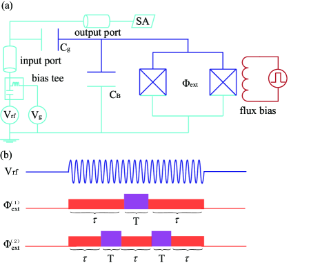
Figure 1: (a) The equivalent circuit network of the transmon qubit and its surroundings. Two parallel Josephson junctions of junction energy $E_{J}$ and capacitance $C_{J}$ are connected to a gate capacitor of capacitance $C_{g}$ and shunted to the ground through a capacitor of capacitance $C_{B}$. The transmon is biased through both a DC offset $V_{g}$ and a magnetic flux $\Phi_{\mathrm{ext}}$. Ramsey biasing is realized through current pulses of particular durations in the flux bias loop. (b) The pulse sequences at the waveguide input and at the flux bias to furnish the Ramsey resonance scheme: $V_{\mathrm{rf}}$ is set to feed a square pulse whose length matches the total time duration of the biasing train; $\Phi_{\mathrm{ext}}^{(1)}$ illustrates the scenario for a double-resonance scheme and $\Phi_{\mathrm{ext}}^{(2)}$ for a triple-resonance scheme. The effectiveness of the two differing schemes for spectroscopy is depicted in the figures below.

To realize the Ramsey biasing scheme, we generate a current pulse train in the bias loop such that $\omega_{eg}(\phi)$ of the qubit is alternatively tuned to its resonance and dispersive regimes with respect to an incident microwave pulse transmitting in the waveguide. The synchronized operation between the pulse-qubit interaction and the bias-tuning follows the illustration in Fig. 1(b). With the contribution from the qubit-field interaction, the full system Hamiltonian containing the qubit-field interaction reads

$$H=\Delta\sigma_{z}+\eta(\sigma_{+}+\sigma_{-})$$ (3)

under the rotating frame $e^{i\omega t}$ of the incident probe field, where $\Delta=(\omega_{eg}-\omega)/2$ is the detuning between the qubit transition frequency $\omega_{eg}$ and the probe field frequency $\omega$. The effective coupling strength $\eta$ depends on the power of the incident microwave pulse. Eq. (3) can be further diagonalized to $H^{\prime}=\lambda\sigma_{z}$ where $\lambda=\sqrt{\Delta^{2}+\eta^{2}}$ with transformation matrix

$$U=\left[\begin{array}[]{cc}\cos\theta/2&-\sin\theta/2\\ \sin\theta/2&\cos\theta/2\end{array}\right]$$ (4)

and transformation angle $\theta=\tan^{-1}(\eta/\Delta)$.

Following the Hamiltonian in the transformed basis, the coefficients $\mathbf{C}^{\prime}(t)=[C_{e}^{\prime}(t)\;C_{g}^{\prime}(t)]$ at the initial state becomes $\mathbf{C}^{\prime}(\tau+t_{0})=\exp\{-i\lambda\sigma_{z}\tau\}\mathbf{C}^{\prime}(t_{0})$ after a time duration $\tau$. Transforming back to the bare-state basis in the laboratory, i.e. $\mathbf{C}(\tau+t_{0})=\exp\{i\omega(\tau+t_{0})\sigma_{z}/2\}U\exp\{-i\lambda\tau\sigma_{z}\}U^{\dagger}\mathbf{C}(t_{0})$, the state coefficients are written as

$$C_{e}(\tau+t_{0})= \left(\cos\lambda\tau-i\cos\theta\sin\lambda\tau\right)e^{-i\omega\tau/2}C_{e}(t_{0}).$$

$$-i\sin\theta\sin\lambda\tau\,e^{-i\omega(\tau/2+t_{0})}C_{g}(t_{0}),$$ (5)

$$C_{g}(\tau+t_{0})= \left(\cos\lambda\tau+i\cos\theta\sin\lambda\tau\right)e^{i\omega\tau/2}C_{g}(t_{0})$$

$$-i\sin\theta\sin\lambda\tau\,e^{i\omega(\tau/2+t_{0})}C_{e}(t_{0}).$$ (6)

With Eqs. (5)-(6), we can consider the variations of coefficients during a time duration $\tau$ when the microwave pulse is controlling the qubit to operate in different regimes. Under the Ramsey scheme, the first operating regime is that of resonance. Hence, without loss of generality, we can assume the initial moment to be $t_{0}=0$, at which the qubit adopts ground state, i.e. $C_{g}(0)=1$ and $C_{e}(0)=0$. After being biased to resonance (flux bias $\phi=0.46$) for a duration $\tau$, the qubit has

$$C_{e}(\tau) =-i\sin\theta\sin\lambda\tau\,e^{-i\omega\tau/2},$$ (7)

$$C_{g}(\tau) =\left(\cos\lambda\tau+i\cos\theta\sin\lambda\tau\right)e^{i\omega\tau/2}.$$ (8)

The second operating regime being dispersive, we consider the approximate Hamiltonian when the qubit is far-detuned from the incident microwave, i.e. $\Delta\gg\eta$ and thus Eq. (3) becomes

$$H\approx H_{D}=\left(\Delta_{D}+\frac{\omega}{2}\right)\sigma_{z}$$ (9)

where $\Delta_{D}=(\omega_{eg}^{\prime}-\omega)/2+\eta^{2}/(\omega_{eg}^{\prime}-\omega)$ is the dispersive qubit-probe detuning at flux bias $\phi^{\prime}=0.49$. The dispersive Hamiltonian only imposes a dynamic phase on the state coefficients during evolution. At the end of a duration $T$ in the dispersive regime after the previous operation at resonance, we then have

$$C_{e,g}(\tau+T)=e^{\mp i(\Delta_{D}+\omega/2)T}C_{e,g}(\tau).$$ (10)

The double-resonance scheme is furnished by biasing the qubit to resonance again for a duration $\tau$, as shown in Fig. 1(b). By compounding Eqs. (7), (8), and (10) and substituting into (5)-(6), we obtain the coefficient of the excited state to be

$$C_{e}(2\tau+T)=-2ie^{-i\omega(\tau+T/2)}\sin\theta\sin\lambda\tau\\ \biggl{\{}\cos\lambda\tau\cos\Delta_{D}T-\cos\theta\sin\lambda\tau\sin\Delta_{D}T\biggr{\}}$$ (11)

at the end of the full bias train and the transition probability across the probe frequency $\omega$ is then computable as $P_{e}=|C_{e}|^{2}$.

III Spectroscopy under double-resonance

Following the expression of Eq. (11), $P_{e}$ is a function of the time lengths $\tau$ and $T$ in addition to the probe frequency $\omega$. For a double-resonance scheme, $2\tau+T$ would be the total probe pulse length and the measurement reading would be the attenuated pulse power of the same length received by the spectrum analyzer (Cf. Fig. 1). Therefore, viewing them as free variables, we can optimize over $\tau$ and $T$ and remove them from the equation. The optimization goal is maximal $P_{e}$ at the resonance frequency with minimum FWHM for the linewidth.

To implement the optimization, we consider $T=R\tau$, i.e. $R$ is a proportional constant indicating the dispersion to resonance time ratio, and that the sampling duration parametrized by $\tau$ is stochastically distributed, which gives the observed transition probability as the time integral of $P_{e}$. The distribution typically adopted for spectroscopic purposes is that of Maxwell Ramsey1950 ; Walstad2013 ,

$$p(x)=e^{-x^{2}}x^{3}.$$ (12)

To make the distribution compatible with the expression of $P_{eg}$, we let the dimensionless $x=\tau/s$, where $s$ is a time constant to be determined. Further, we write $|C_{e}|^{2}$ as a function of $\tau$ in terms of a sum of cosines to simplify the integrand. This is possible when we observe from Eq. (11) that the factors containing $\lambda\tau$, $\omega\tau$, and $R\Delta_{D}\tau$ can all be reduced to cosines or combinations of cosines and constants.

Therefore, in terms of the integral

$$I_{s}(\beta)=\int_{0}^{\infty}dx\,e^{-x^{2}}x^{3}\cos(2\beta sx),$$ (13)

where $sx$ is equivalent to the time variable and $\beta$ denotes the various frequency terms, the weighted average of $|C_{e}|^{2}$ is

$$\left\langle P_{e}\right\rangle=\frac{F^{\prime 4}+4F^{2}}{4}+\frac{F^{\prime 4}-2F^{2}}{2}I_{s}(R\Delta_{D})$$

$$-2F^{2}I_{s}(\lambda)-\frac{F^{\prime 4}}{2}I_{s}(2\lambda)$$

$$+\left(F+F^{\prime}\right)\left[FI_{s}\left(\lambda+R\Delta_{D}\right)-\frac{(F+F^{\prime})}{4}I_{s}\left(2\lambda+R\Delta_{D}\right)\right]$$

$$+\left(F-F^{\prime}\right)\left[FI_{s}\left(\lambda-R\Delta_{D}\right)-\frac{(F-F^{\prime})}{4}I_{s}\left(2\lambda-R\Delta_{D}\right)\right]$$ (14)

where we used the abbreviations

$$F =\frac{\eta\Delta}{\lambda^{2}},\qquad F^{\prime}=\frac{\eta}{\lambda}.$$ (15)

To optimize for a maximal $\left\langle P_{e}(\omega)\right\rangle$ at the qubit resonance frequency, we consider tuning the integral $I_{s}$, which contribute both positive and negative terms in Eq. (14). Since the constant term in Eq. (14) is positive, we minimize the magnitude of $I_{s}$ to opt for a maximal $\left\langle P_{e}\right\rangle$ overall. Following the expression of Eq. (13), the integrand of $I_{s}$ obtains its minimum value at $\beta s\approx 0.68\pi$. Further, about close-resonance limit where we regard $\Delta=0$ and thus $\lambda=\eta$, Eq. (14) contains the integrals $I_{s}(\eta)$ and $I_{s}(2\eta)$, whose coefficients are negative, in addition to the $\omega$-dependent integrals. The optimization is obtained, therefore, by minimizing these two $\omega$-independent integrals. Obviously, they cannot be simultaneously minimized at the same $s$ value, so we determine numerically the compromised time constant $s$ that leads to a maximal peak value with minimal FWHM.

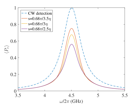
Figure 2: (Color online) The transition probability of a transmon qubit as a function of probe field frequency $\omega/2\pi$ at three values of $s$ between $0.68\pi/3.5\eta$ and $0.68\pi/2.5\eta$, given as the family of solid curves. The blue dashed line, which corresponds to the spectrum of CW detection under the same system parameters, serves as a reference. 

Figure 2 plots the transition probability $\left\langle P_{e}\right\rangle$ of a transmon qubit against the probe frequency $\omega$ at various values of $s$ under the proposed Ramsey-biased scheme. The energy ratio $E_{J}/E_{C}$ of the transmon is set to $100$. The two distinct flux biases during the double-resonance process are given as above. The coupling strength is assumed to be $\eta/2\pi=100\mathrm{MHz}$. The resonance peak, which occurs at $4.505\mathrm{GHz}$, is obtained at the optimized $T$ to $\tau$ ratio $R=0.001$. Compared to the transition spectrum according to CW detection (shown as the dashed curve), the new scheme provides an improved FWHM at all values of $s$. In particular, at $s=0.68\pi/3\eta$, FWHM is reduced to $306\mathrm{MHz}$ from $400\mathrm{MHz}$ of the CW detection ($\approx 23\%$ reduction), given the cost of a slightly reduced peak magnitude, demonstrating the advantage of the Ramsey-biased scheme. For all values of $s$, the shift in frequency due to dispersion is about $1.7$ MHz from CW detection, which is almost negligible compared to the resonance frequency.

IV Spectroscopy under triple-resonance

To further optimize the transition spectrum, i.e. to obtain a curve with a narrower linewidth to those shown in Fig. 2, we consider a triple-resonance scheme. Instead of the $\tau$-$T$-$\tau$ segmentation for the qubit-pulse interaction, we consider three segments of $\tau$, during which the qubit is resonant, and two segments of $T$, during which the qubit is dispersive. Again, the two operating regimes are interlacing with each other and we can reuse Eqs. (5)-(6) and (10). Applying them on Eqs. (11), we obtain the coefficient

$$C_{e}(3\tau+2T)= -ie^{-i\omega(3\tau/2+T)}\sin\theta\sin\lambda\tau\times$$

$$\Bigl{\{}2\left(\cos^{2}\lambda\tau-\cos^{2}\theta\sin^{2}\lambda\tau\right)\cos 2\Delta_{D}T$$

$$-2\cos\theta\sin 2\lambda\tau\sin 2\Delta_{D}T$$

$$+\cos^{2}\lambda\tau+\cos 2\theta\sin^{2}\lambda\tau\Bigr{\}}.$$ (16)

of the excited state at the end of the pulse train.

The expression of $C_{e}$ is much more complicated for the triple resonance scheme than that given in Eq. (11). Before reducing the terms of $|C_{e}|^{2}$ to cosines to carry out the integration in Eq. (13), we simplify the expression of Eq. (16) to examine the analytical dependence only in the close-resonance region. We again let $T=R\tau$ ($R$ to be determined similarly to Sec. III) and regard $C_{e}$ again as a function of $\tau$, which will be integrated out. At $\Delta\to 0$ such that all $\cos^{n}\theta$ terms vanish, we have

$$\left\langle P_{e}^{\mathrm{res}}\right\rangle =\frac{F^{\prime 2}}{16}\Bigl{\{}6-10I_{s}(\lambda)+4I_{s}(2\lambda)-6I_{s}(3\lambda)$$

$$+4I_{s}(2R\Delta_{D})+4I_{s}(\lambda+R\Delta_{D})+4I_{s}(\lambda-R\Delta_{D})$$

$$+I_{s}(\lambda+2R\Delta_{D})+I_{s}(\lambda-2R\Delta_{D})$$

$$-2I_{s}(2\lambda+2R\Delta_{D})-2I_{s}(2\lambda-2R\Delta_{D})$$

$$-4I_{s}(3\lambda+R\Delta_{D})-4I_{s}(3\lambda-R\Delta_{D})$$

$$-I_{s}(3\lambda+2R\Delta_{D})-I_{s}(3\lambda-2R\Delta_{D})\Bigr{\}}.$$ (17)

Comparing Eq. (17) with Eq. (14), one sees that the extra segment of resonance effectively contributes extra terms of frequency $3\lambda$. Like $2\lambda$-frequency terms in Eq. (14), these triple-frequency terms all have negative weights, thus reducing the probability magnitude at frequencies distant from resonance. Cutting down the magnitude naturally leads to a narrower resonance peak. $\left\langle P_{e}\right\rangle$ computed directly as $|C_{e}|^{2}$ under the triple-resonance scheme is plotted in Fig. 3(a) for three optimized values of $s$, against the double-resonance result for $s=0.68\pi/3\eta$. The optimization is obtained under $T$ to $\tau$ ratio $R=0.045$. For $s=0.68\pi/2\eta$, the triple-resonance scheme has a FWHM of $193$ MHz, i.e. a further $37\%$ reduction over the double-resonance case, albeit the compromise at the peak absorption magnitude.

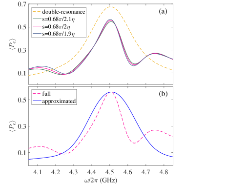
Figure 3: (Color online) (a) The transition probability under the triple-resonance scheme at three different values of $s$ (solid curves) compared to the double-resonance scheme (dashed curve, $s=0.68\pi/3\eta$). (b) $\left\langle P_{e}^{\mathrm{res}}\right\rangle$ under close-resonance approximation $s=0.68\pi/2\eta$ (solid curve) compared to one without approximation (dashed curve). 

The resonance peak, like that of Fig. 2, experiences negligible dispersion shift but exhibits sideband fringes. These fringes, unlike those in the original Ramsey spectroscopy scheme, are flattened and asymmetric. To examine the effectiveness of $\left\langle P_{e}^{\mathrm{res}}\right\rangle$, it is plotted against the full numerical result in Fig. 3(b) with the same values of $s$ and $R$. The approximation coincides with the analytical expression at close-resonance range but falls short at estimating the spectral width. At off-resonance range, the terms associated with high-order $\cos^{n}\theta$ coefficients are integrals $I_{s}$ of frequency higher than $3\lambda$. Since these terms are also negative, $\left\langle P_{e}\right\rangle$ at frequencies distant from resonance falls off more sharply than that expected by Eq. 17, which omit these terms. Consequently, the fringes that are caused by higher-order secondary photon processes are also omitted.

V Conclusions

We generalize Ramsey’s spectroscopic method of transition detection, which was applied to atoms traveling through optical cavities, to detecting superconducting qubits on solid-state circuits. In this multi-segment resonance scheme, the time segment originally reserved for free atomic evolution is replaced by a dispersion operation for the qubit, which give rises not only to a narrowed linewidth of transition spectrum, but also to an elimination of side fringes. We have proved that the unwanted frequency shift in the detection due to dispersion is negligible when the ratio of time segment arrangments are suitably optimized. The linewidth narrowing can be further improved when extra resonance segments are added.

- (1) J. E. Mooij, T. P. Orlando, L. Levitov, L. Tian, C. H. van der Wal, and S. Lloyd, Science 285, 1036 (1999).
- (2) J. Clarke and F. K. Wilhelm, Nature 453, 1031 (2008).
- (3) Y. Nakamura, C. D. Chen, and J. S. Tsai, Phys. Rev. Lett. 79, 2328 (1997).
- (4) T. P. Orlando, et al., Phys. Rev. B 60, 15398 (1999).
- (5) C. H. van der Wal, et al. , Science 290, 773 (2000).
- (6) J. M. Martinis, S. Nam, J. Aumentado, and C. Urbina, Phys. Rev. Lett. 89, 117901 (2002).
- (7) M. A. Kastner, Phys. Today 46, 24 (1993).
- (8) J. Q. You and F. Nori, Phys. Today 58, 42 (2005).
- (9) I. Chiorescu, Y. Nakamura, C. J. P. M. Harmans, and J. E. Mooij, Science 299, 1869 (2003).
- (10) A. Wallraff, et al., Nature 431, 162 (2004).
- (11) J.-T. Shen and S. Fan, Phys. Rev. Lett. 95, 213001 (2005).
- (12) T. Hime, et al., Science 314, 1427 (2006).
- (13) S. N. Shevchenko, et al., Phys. Rev. B 78, 174527 (2008).
- (14) H. C. Torrey, Phys. Rev. 59, 293 (1941).
- (15) N. F. Ramsey, Phys. Rev. 78, 695 (1950).
- (16) H. Abele, T. Jenke, H. Leeb, and J. Schmiedmayer, Phys. Rev. D 81, 065019 (2010).
- (17) T. Zanon-Willette, V. I. Yudin, and A. V. Taichenachev, Phys. Rev. A 92, 023416 (2015).
- (18) J. Koch, et al., Phys. Rev. A 76, 042319 (2007).
- (19) S. Filipp, et al., Phys. Rev. Lett. 102, 200402 (2009).
- (20) A. Walstad, American Journal of Physics 81, 555 (2013).
- (21) F. Yan, et al., Phys. Rev. B 85, 174521 (2012).
- (22) F. Yan, et al., Nat. Commun. 4, 1 (2013).
- (23) J. A. Schreier, et al., Phys. Rev. B 77, 180502 (2008).
- (24) J. M. Fink, et al., Phys. Rev. Lett. 103, 083601 (2009).