Dipartimento di Fisica e Astronomia

Dottorato di Ricerca in Fisica e Astronomia
Indirizzo Fisica - XXXII Ciclo
Settore Scientifico Disciplinare: FIS/02
Thermodynamic equilibrium of massless fermions with vorticity, chirality and magnetic field
Matteo Buzzegoli

Supervisor:
Prof. Francesco Becattini

Coordinator of PhD program:
Prof. Raffaello D’Alessandro

Academics years 2016-2019

Notation and conventions

In this work we mostly use the natural unit system in which $\hslash=c=G=k_{B}=1$.

The Minkowski metric is defined by the tensor $\eta_{\mu\nu}=$diag$(1,-1,-1,-1)$ with greek indices running on four-vectors components $\mu=0,1,2,3$; instead we use latin indices for space coordinates only $i=1,2,3$ and we adopt the Einstein index summation convention but only if at least one repeated index is up and the other is down.

The four-vectors and the tensors in general are indicated both with their components (e.g. $\beta^{\mu}$) and their symbol (e.g. $\beta$), instead the tri-vectors are indicated with their component (e.g. $k^{i}$) or with a bold letter (e.g. $\textstyle\mathbf{k}$). The module of the four-vector is indicated as $\left|\beta\right|$ or $\sqrt{\beta^{2}}$. The inner product is generally indicated with “$\,\cdot\,$”, the same symbol is used for the contraction of two indices of two tensors between the most right of the first with the most left of the second (e.g. $(\alpha\cdot\varpi)_{\mu}=\alpha_{\lambda}\varpi^{\lambda\mu}$). We use the symbol “$\wedge$” for the wedge product.

The sansserif letters are used to indicate the element of a group (e.g. $\mathsf{R}\in$ SO(3)). If it is not explicitly marked, the stress-energy tensor $\widehat{T}_{\mu\nu}$ is symmetric.

We use Weyl (chiral) basis for Gamma matrices $\gamma^{\mu}$; in imaginary time we denote Euclidean Gamma matrices with $\tilde{\gamma}_{\mu}$ and when it is clear that we switched into imaginary formalism the tilde symbol is omitted; in curved spacetime we define the coordinate dependent Dirac gamma matrices as $\underline{\gamma}^{\mu}(x)\equiv e_{a}^{\,\,\mu}(x)\gamma^{a}$, where $e_{a}^{\,\,\mu}(x)$ is the vierbein field.

The following special symbols and abbreviations are used throughout:

${\rm i}$	imaginary unit;
$\mathrm{e}$	Euler’s number;
$*$	complex conjugate;
$\dagger$ or h.c.	Hermitian conjugate;
$\bar{\,}$	Dirac adjoint (e.g. $\bar{\psi}$);
$\widehat{\;}$	quantum operator (e.g. $\widehat{T}^{\mu\nu}$);
$\hat{}$	versor (e.g. $\hat{u}$);
Re (Im)	real (imaginary) part;
${\text{tr}},\,\log,\,\det$	trace, natural logarithm, determinant;
$\left[A,B\right]$	commutator $AB-BA$;
$\left\{A,B\right\}$	anticommutator $AB+BA$;
$\mathop{:\!{\,}\!:}$	normal ordering;
$a_{(\mu,\nu)}$	symmetric sum on index $\frac{1}{2}(a_{\mu,\nu}+a_{\nu,\mu})$;
$\epsilon^{\mu\nu\rho\sigma}$	Levi-Civita symbol such that $\epsilon^{0123}=+1$;
$\frac{\partial}{\partial x^{\mu}}$ or $\partial_{\mu}$	partial derivative;
$g_{\mu\nu},\,g\equiv\det(g_{\mu\nu})$	curved spacetime metric with inverse metric $g^{\mu\nu}$;
$\Gamma^{\lambda}_{\,\mu\nu}=\Gamma^{\lambda}_{\,\nu\mu}=\frac{1}{2}g^{\lambda\sigma}\left(g_{\sigma\nu,\mu}+g_{\mu\sigma,\nu}-g_{\mu\nu,\sigma}\right)$	Christoffel connection;
$\nabla_{\mu}$	covariant derivative;
$R^{\lambda}_{\,\tau\mu\nu}=\Gamma^{\lambda}_{\,\tau\mu,\nu}-\Gamma^{\lambda}_{\,\tau\nu,\mu}+\Gamma^{\lambda}_{\,\nu\sigma}\Gamma^{\sigma}_{\,\tau\mu}-\Gamma^{\lambda}_{\,\mu\sigma}\Gamma^{\sigma}_{\,\tau\nu}$	Riemann tensor;
$R_{\mu\nu}=R^{\alpha}_{\,\mu\alpha\nu}$	Ricci tensor;
$\simeq$	approximately equal to;
$\sim$	order of magnitude estimate;
$\approx$	asymptotically approximate to;
$\equiv$	defined to be equal to;
$\tau=\!{\rm i}\,t,\quad X\equiv(\tau,x^{i})$	Euclidean coordinates;
$\int_{X}\equiv\int_{0}^{\beta}\mathrm{d}\tau\int_{\mathchoice{\mbox{\boldmath$\displaystyle\mathbf{x}$}}{\mbox{\boldmath$\textstyle\mathbf{x}$}}{\mbox{\boldmath$\scriptstyle\mathbf{x}$}}{\mbox{\boldmath$\scriptscriptstyle\mathbf{x}$}}},\quad\int_{\mathchoice{\mbox{\boldmath$\displaystyle\mathbf{x}$}}{\mbox{\boldmath$\textstyle\mathbf{x}$}}{\mbox{\boldmath$\scriptstyle\mathbf{x}$}}{\mbox{\boldmath$\scriptscriptstyle\mathbf{x}$}}}\equiv\int\mathrm{d}^{d}\mathchoice{\mbox{\boldmath$\displaystyle\mathbf{x}$}}{\mbox{\boldmath$\textstyle\mathbf{x}$}}{\mbox{\boldmath$\scriptstyle\mathbf{x}$}}{\mbox{\boldmath$\scriptscriptstyle\mathbf{x}$}}$	integral in Euclidean space-times where $\beta\equiv 1/T$, and $d=3$ is the space dimensionality;
$K\equiv(k_{n},k_{i}),\quad$ sometimes $\omega_{n}=k_{n}$	Fourier modes in Matsubara formalism;
$\operatorname*{\mathchoice{\ooalign{$\displaystyle\sum$\cr$\displaystyle\int$\cr}}{\ooalign{\raisebox{0.14pt}{\scalebox{0.7}{$\textstyle\sum$}}\cr$\textstyle\int$\cr}}{\ooalign{\raisebox{0.2pt}{\scalebox{0.6}{$\scriptstyle\sum$}}\cr$\scriptstyle\int$\cr}}{\ooalign{\raisebox{0.2pt}{\scalebox{0.6}{$\scriptstyle\sum$}}\cr$\scriptstyle\int$\cr}}}_{K}\equiv T\sum_{k_{n}}\int_{\mathchoice{\mbox{\boldmath$\displaystyle\mathbf{k}$}}{\mbox{\boldmath$\textstyle\mathbf{k}$}}{\mbox{\boldmath$\scriptstyle\mathbf{k}$}}{\mbox{\boldmath$\scriptscriptstyle\mathbf{k}$}}},\quad\int_{\mathchoice{\mbox{\boldmath$\displaystyle\mathbf{k}$}}{\mbox{\boldmath$\textstyle\mathbf{k}$}}{\mbox{\boldmath$\scriptstyle\mathbf{k}$}}{\mbox{\boldmath$\scriptscriptstyle\mathbf{k}$}}}\equiv\int\mathrm{d}^{k}\mathchoice{\mbox{\boldmath$\displaystyle\mathbf{k}$}}{\mbox{\boldmath$\textstyle\mathbf{k}$}}{\mbox{\boldmath$\scriptstyle\mathbf{k}$}}{\mbox{\boldmath$\scriptscriptstyle\mathbf{k}$}}/(2\pi)^{d}$	Fourier-analysis in Matsubara formalism;
$\operatorname*{\mathchoice{\ooalign{$\displaystyle\sum$\cr$\displaystyle\int$\cr}}{\ooalign{\raisebox{0.14pt}{\scalebox{0.7}{$\textstyle\sum$}}\cr$\textstyle\int$\cr}}{\ooalign{\raisebox{0.2pt}{\scalebox{0.6}{$\scriptstyle\sum$}}\cr$\scriptstyle\int$\cr}}{\ooalign{\raisebox{0.2pt}{\scalebox{0.6}{$\scriptstyle\sum$}}\cr$\scriptstyle\int$\cr}}}_{\{K\}}\equiv T\sum_{\{k_{n}\}}\int_{\mathchoice{\mbox{\boldmath$\displaystyle\mathbf{k}$}}{\mbox{\boldmath$\textstyle\mathbf{k}$}}{\mbox{\boldmath$\scriptstyle\mathbf{k}$}}{\mbox{\boldmath$\scriptscriptstyle\mathbf{k}$}}}$	antiperiodic (or fermionic) summation ;
$n_{\textup{F}}(x)=\frac{1}{\mathrm{e}^{\beta x}+1}$	Fermi-Dirac distribution function;
$n_{\textup{B}}(x)=\frac{1}{\mathrm{e}^{\beta x}-1}$	Bose-Einstein distribution function;
$\zeta(z)$	Riemann zeta function;
$\Gamma(z)$	Euler gamma function;
$D_{n}(z)$	parabolic cylinder function.

Other notation is introduced as needed.

Introduction

The quantum behavior of a physical system is usually relevant at microscopic lengths, while the classical behavior is recovered at macroscopic scales. However, quantum properties may emerge even at macroscopic scale, giving rise to phenomena not allowed in a classical world. Some notable instances are superfluidity, superconductivity, ultra-cold atom gases and quantum Hall effects. In the last decades, these macroscopic quantum phenomena have produced great advances both in theoretical and in technological fields.

Macroscopic quantities are understood as emergent properties of a system and are obtained integrating out all the detailed information about microscopic dynamics but retaining collective behavior. For example, the temperature $T$ measures the mean kinetic energy of the system constituents, which is roughly given by $k_{B}T$, where $k_{B}$ is the Boltzmann constant. While temperature gives the scale of macroscopic quantities, the (reduced) Planck constant $\hbar$ sets the scale for quantum behavior. For instance, consider a Bose-Einstein condensate, which is required for most of the aforementioned phenomena. In that case, for a fluid with particle density $\rho$ and consisting of mass $m$ bosons, we can associate a quantum energy $\hbar^{2}\rho^{2/3}/m$. Indeed, boson fluids show quantum behavior (the condensate) when this energy is larger than the thermal energy $k_{B}T$. That is why all the aforementioned phenomena require low-temperature environments to keep the quantum effects dominant.

Since most of the systems in nature are affected by rotation or by acceleration, such as the one caused by Earth gravitational attraction, we may wonder if an interplay between angular velocity $\omega$, or acceleration $a$, and quantum effects may produce macroscopic phenomena. Indicating with $c$ the speed of light in vacuum, this is likely to occur if the quantum energy associated to angular velocity $\hbar\,\omega$ or to acceleration $\hbar\,a/c$ is larger than thermal energy $k_{B}T$, i.e. when the following ratios $w$ and $\alpha$ become relevant:

$$w\equiv\frac{\hbar\,\omega}{k_{B}T},\quad\alpha\equiv\frac{\hbar\,a}{c\,k_{B}T}.$$

When replacing some numbers related to “common” physical systems, we realize that $\alpha$ and $w$ are usually frighteningly small: $\alpha,\,w\sim 10^{-20}$. However, nature and humans resourcefulness provided some instances of matter under extreme conditions where those parameters play a significant role.

With the Relativistic Heavy Ion Collider at Brookhaven National Laboratory and with the Large Hadron Collider at CERN, ions of heavy nuclei (usually Au and Pb) are collided between themselves at ultra-relativistic speed. As a result, a new state of nuclear matter, dubbed the Quark-Gluon Plasma (QGP), is created [1]. The QGP phase occurs at extremely high temperatures and densities when the hadrons dissolve into an asymptotically free state of their elementary constituents: quarks and gluons. The QGP phase produced in high energy nuclear collisions lasts for about 5 fm$/c\simeq 10^{-23}$ s. During that time it expands and cools down until it once again forms hadron states, which are then detected by instruments. Even the Universe, some picoseconds after the Big Bang and lasting for 10 microseconds, is thought to have taken the form of quark-gluon plasma. This new phase of matter has become a great benchmark for phase transitions, symmetries breaking, collective behavior and baryonic asymmetry inside the Standard Model of elementary particles, especially for Quantum Chromo-Dynamics (QCD), the theory that describes nuclear interactions.

QCD possesses the remarkable property of asymptotic freedom, meaning that at short distances, the QCD running coupling constant is small and quantities can be reliably evaluated in perturbation theory. However, at strong coupling, we still lack a reliable theoretical method for performing analytical calculations. As a consequence, despite QCD has well-known symmetries and established elementary constituents, its emergent behavior remains a mystery to us. For instance, perturbation theory does not contain confinement of color, i.e. it does not explain how the asymptotic states of QCD perturbation theory (colored quarks and gluons) transform into the asymptotic states actually observed in experiments (the color-singlet hadrons). The confinement scale can be estimated from the proton radius, roughly 1 fm, which corresponds to an energy $\Lambda$ of about 200 MeV. Color confinement can be overcome rising the temperature above a critical value $T_{c}$; intuitively when it reaches confinement energy $k_{B}T_{c}\sim\Lambda$ (lattice calculations indicate $k_{B}T_{c}=154\pm 8$ MeV [2]), then one obtains a gas composed by almost free quarks and gluons, the aforementioned QGP. For the same critical value, the weakly broken chiral symmetry, responsible for the three light pions, gets restored.

Experiments already revealed and established remarkable properties of the QGP. Regarding collective behavior, it is found that the QGP is indeed a fluid and what’s more the one with the lowest viscosity ever observed [3, 4]. Moreover, most of the collisions are not central and so produce matter with angular momentum of order $1000\hbar$. This vorticity couples with quantum behavior with an energy associated to acceleration of $\hbar\,a/c\sim 10$ MeV and to rotation of $\hbar\,\omega\sim 12$ MeV [5]. Compared to the thermal energy of the plasma $k_{B}T\sim 200$ MeV, this means a ratios of $\alpha=0.05$ and $w=0.06$. In agreement with local thermodynamic equilibrium predictions [6], these values of local vorticity and acceleration are sufficient to induce polarization on the particles produced by the plasma, as recent measures on Lambda particle polarization have confirmed [5, 7]. This, beside vesting QGP as the most vorticous fluid ever observed, is the proof that quantum effects induced by rotation are displayed at a macroscopic level even at extremely high temperatures.

In recent years, studies on the interplay of quantum effects with vorticity and magnetic field identified several novel non-dissipative transport phenomena [8] similar to the effects that lead to particle polarization. The phenomenology is even richer in systems possessing chiral fermions. Elementary particles are classified according to the Lorentz group, which has two unitarily inequivalent spinor representations related by parity transformation. A particle is said to have right or left chirality if it belongs to one or the other of such representations. Or, in other words, a particle is chiral if it is possible to distinguish the particle from its mirror image. The identification is easier for massless spin $1/2$ fermions because in this case chirality corresponds to particle helicity, which is whether the particle spin is or is not aligned with the particle momentum.

Among those non-dissipative transport phenomena, the Chiral Magnetic Effect (CME) [9] is the induced electric current along an external magnetic field driven by chiral imbalance. Since both the magnetic field and the electric current are odd quantities under time reversal transformation $\mathsf{T}$, the CME conductivity must be $\mathsf{T}$-even, revealing that its occurrence does not involve any dissipative process. On the contrary, the magnetic field is even under parity transformation $\mathsf{P}$ but the electric current is $\mathsf{P}$-odd. This is why to connect the two we need a chiral medium: matter possessing an imbalance between right- and left-handed particles.

An instance of chiral matter is once again found in QGP, where chirality is thought to be generated in the topological sector of QCD vacuum states. The compactness of SU(3) group, not addressed in perturbative approaches, allows the existence of nontrivial topological solutions of gluon configurations. These solutions can possess chirality which can be transferred to quarks through the chiral anomaly. Indeed, the Atiyah-Singer index theorem relates the topological charge of the background gauge field configuration to the number of fermionic zero-modes of the Dirac operator. Since quarks also possess electric charge, we can probe their topology using a magnetic field.

In heavy-ion collisions, together with the QGP, a magnetic field is generated with an initial magnitude of $eB\sim 10m_{\pi}^{2}\sim 10^{18}$ G [10, 11, 12]. Actually, it is the strongest magnetic field in the present Universe, thousands of times stronger than those found on the surface of magnetars, where it may also affect its cold dense nuclear matter. In QGP produced by heavy-ion collisions, we then have all the ingredients for the generation of CME, and its observable manifestation would be the proof of the existence of topological structure of QCD. CME is expected to cause a charge-dependent azimuthal asymmetry on the spectrum of produced particles, which has already been observed by STAR Collaboration at RHIC [13]. However, mundane backgrounds unrelated to the CME may be able to explain the observed charge separation and dedicated experiments with isobar collisions [14] are currently ongoing to asses this possibility. Moreover, contrary to angular velocity, which persists longer in the plasma due to angular momentum conservation, the magnetic field has a very short lifetime, about $\sim 10^{-23}$ s, and there are still significant theoretical uncertainties due to its evolution. That is why recently many efforts have been made to develop a proper chiral magnetohydrodynamics [15, 16, 17] to run simulations in which both the medium and the field are evolved dynamically.

Magnetic field has already been successfully used to probe topological properties, as in the case of (fractional) quantum Hall effect in condensed matter physics. It is then not surprising that thanks to the discovery of chiral materials (Dirac and Weyl semimetals), CME has received its experimental evidence in condensed matter [18]. In those materials, chirality is pumped into the system with an external parallel magnetic and electric field by leveraging chiral anomaly. This reinforces the idea that the CME coefficient is entirely dictated by chiral anomaly and, because of that, is topologically protected. Indeed various computations in severals regime from free to strongly coupled systems found the same conductivity for CME independently of dynamical details.

We refer to quantum anomalies when a classical symmetry of a theory is not compatible with quantum theory. When massless quarks are addressed, QCD is invariant under chiral transformations and, for Noether’s theorem, the axial current is conserved. However, this symmetry is explicitly broken by the regularization of quantum processes in background gauge fields [19]. Among several consequences, chiral anomaly is responsible for the large mass of the pseudoscalar $\eta^{\prime}$ meson and for the decay of neutral pion into two photons. The salient feature of quantum anomalies is that they bridge collective motion of particles with arbitrarily large momenta in the vacuum to the finite momentum world [20]. That is how quantum anomalies can possibly affect macroscopic phenomena, even though the latter involves a large number of quanta. Moreover, the strength of anomalies resides on the non-renormalization theorem [19], stating that the anomaly is exact as an operator relation at one loop.

Quantum anomalies have a primary role in the understanding (and in the discovery) of non-dissipative phenomena of quantum many-body physics we are discussing. We already mentioned CME and its role in heavy-ion collisions; in astrophysics transport phenomena induced by anomalies could explain the sudden acceleration during the birth of neutron stars (neutron star kicks) [21] and in cosmology the origin of primordial magnetic fields [22]. Chiral anomaly also induces macroscopic effects when coupling with vorticity. For example, the Chiral Vortical Effect (CVE) is the generation of an electric current along the global rotation in a chiral medium. This effect shares many properties with CME and has similar consequences on the phenomenology of QGP, although, being CVE independent of charge, the two effects can be distinguished.

Connections and similarities between rotation and magnetic field have a long history, starting from noticing that a charged particle under magnetic force undergoes into a circular motion, to the Barnett and Einstein-de Hass effects. Spin-orbit coupling can transfer angular momentum to spin and vice versa. Therefore, in ferromagnetic materials, mechanical rotation can induce magnetization (Barnett effect) and, due to angular momentum conservation, also a variation on magnetization induces rotation (Einstein-de Haas effect). It has been suggested that CVE could be interpreted as an extension of a relativistic Barnett effect, see [23].

For the sake of understanding, it is important to make a clear distinction between CVE and another macroscopic quantum phenomena: the Axial Vortical Effect (AVE), which is the induced axial current along the global rotation. Contrary to electric current, the axial current has a tight connection with both chirality and spin. In relativistic theories axial current is dual to spin tensor and in systems consisting of massless fermions and without background gauge fields, the global chiral charge is defined as the integral of axial current. Other substantial differences with CVE are that AVE does not require a chiral imbalance and that it is not entirely topologically protected [24], questioning its possible proposed relation with mixed-axial gravitational anomaly [25].

In this work, we consider thermodynamic properties of systems composed by massless fermions with a chiral imbalance and subject to global vorticity and external magnetic field. The systematic derivations of all constitutive equations are carried out using the covariant operator approach [26] based on Zubarev method of stationary non-equilibrium density operator [27, 28, 29]. With this procedure, the underlying theory has full-quantum properties and does not breaks down when a kinetic description is no longer valid. Indeed, close to the critical temperature, the QGP constituents are strongly interacting and the mean free path length is comparable to the quantum oscillations of the fields, hindering a kinetic description in terms of quasiparticles. Moreover, the effects of global vorticity in this formalism arise naturally from the covariance properties of the density matrix.

The arguments in the thesis are divided as follows. An introduction to quantum relativistic statistical mechanics is provided in Chapter 1. In particular, the key concept for this work is the global thermal equilibrium in the presence of vorticity, which is given in Section 1.4. The chiral anomaly is introduced in Section 1.2, where we also define a conserved current via the Chern-Simons current. A chiral conserved current is needed to reach global equilibrium with chiral imbalance when dynamic or external gauge fields are considered. The issue of a conserved axial current is discussed again in Section 4.3 for external electromagnetic field and in Section 4.4 for dynamical gauge fields. Global equilibrium with both chiral imbalance and vorticity is considered in Section 1.4. In chapter 2, we review the finite temperature field theory methods for fermions and gauge fields. In Section 2.4, we address thermodynamics of massless fermions at finite density and finite chirality.

In chapter 3, we discuss the global equilibrium of massless fermions in a chiral vorticous medium. We provide thermodynamic constitutive equations at the second-order of thermal vorticity for relevant physical quantities, such as the stress-energy tensor and both axial and electric currents. In Section 3.3, we evaluate thermal coefficients up to second order in thermal vorticity for the case of free fermions.

In chapter 4, we consider global vorticous thermal equilibrium in presence of an external electromagnetic field. First, in Section 4.1, we review the properties of fermions under external electromagnetic field; in particular (Section 4.1.1) how translation and Lorentz generators are affected. Then, in Section 4.2, we provide exact solutions for the thermodynamics of non-interacting chiral fermions subject to a constant magnetic field but with vanishing thermal vorticity. Then, in Section 4.3, we discuss the general properties of thermal equilibrium with both external electromagnetic field and thermal vorticity and we give constitutive equations as an expansion of only thermal vorticity. In Section 4.3.2, we derive the effects of electromagnetic field on first order thermal coefficients using the conservation equations of operators. At last, in Section 4.4, we consider dynamic gauge fields and we show that the AVE receives radiative corrections.

1  Quantum relativistic statistical mechanics

In this work, we deal with global thermodynamic equilibrium of relativistic quantum systems. In this chapter, we review how to derive macroscopic behavior at thermal equilibrium using the methods of statistical mechanics in a full quantum relativistic framework. We are using the method of non-equilibrium statistical operator introduced by Zubarev [27] and later reworked by van Weert [30], see [29] for a revision of original arguments. Zubarev’s method provides a stationary statistical operator, which is then well-suited to be used in relativistic quantum field theory in Heisenberg representation. Therefore, this method can be used to describe systems that reached local thermal equilibrium and to derive their hydrodynamic evolution. These are the main reasons why recently Zubarev’s method has been adopted in [26, 31] and in sequent works to derive quantum effects on relativistic systems.

Before turning on relativistic system, we briefly summarize how global equilibrium is recovered in quantum statistical mechanics using the principle of maximum information entropy. Global thermodynamic equilibrium is described as a static statistical ensembles of systems which are only defined by the specification of macroscopic variables. The statistical operator (also called density matrix) $\widehat{\rho}$ provides the “statistical mixture” and it is given by

$$\widehat{\rho}=\sum_{n}p_{n}|n\rangle\langle n|,\quad\sum_{n}p_{n}=1,$$

where the $p_{n}$’s are the statistical weight of $n$th state and the $\{|n\rangle\}$’s form a complete set. Starting from the statistical operator one calculates various quantities related to thermal equilibrium, such as the partition function, the Green’s functions and the Wigner function. Average value of an observable related to the quantum operator $\widehat{O}$ is simply obtained as

$$\langle\,\widehat{O}\,\rangle={\text{tr}}(\widehat{\rho}\,\widehat{O})=\sum_{n}p_{n}\langle n|\widehat{O}|n\rangle.$$

At global equilibrium, the density matrix operator gives the stationary thermal states of the system; therefore, it can only depend on conserved quantities. In Newtonian physics, there exist seven first integrals related to the conservation of energy, momentum and angular velocity. To these constants, other conserved quantities can be added, such as the particle number, the baryon number and the electric charge.

The maximum entropy principle provides a methods to build the density matrix appropriate to the system we are considering. For instance, in the canonical ensemble only the Hamiltonian $\widehat{H}$ and a conserve charge $\widehat{Q}$ are taken in account. In general, we can add any amount of conserved quantities as long as the statistical operator remains time-independent. It is postulated [32] that the equilibrium state maximizes the Von Neumann entropy or information entropy

$$S[\,\widehat{\rho}\,]=-{\text{tr}}(\widehat{\rho}\log\widehat{\rho})$$

under the following constraints

$$\langle\widehat{H}\rangle=E=\text{constant},\quad\langle\widehat{Q}\rangle=Q=\text{constant},\quad{\text{tr}}\left(\,\widehat{\rho}\,\right)=1.$$

In order to take into account the constraints, we use the method of Lagrange multipliers, which translates our problem to the extremization of the free energy functional $F$ with respect to $\widehat{\rho}$:

$$F_{\beta,\zeta,\lambda_{0}}[\,\widehat{\rho}\,]=-{\text{tr}}(\widehat{\rho}\log\widehat{\rho})-\beta[{\text{tr}}(\widehat{\rho}\,\widehat{H})-E]+\zeta[{\text{tr}}(\widehat{\rho}\,\widehat{Q})-Q]-\lambda_{0}[{\text{tr}}(\widehat{\rho})-1]$$

where $\beta$, $\zeta$ and $\lambda_{0}$ are respectively the Lagrange multiplier conjugate of energy $E$, charge $Q$ and to normalization. The maximal solution [32] is the well known Gibbs distribution

$$\widehat{\rho}=\frac{1}{\mathcal{Z}}\mathrm{e}^{-\beta\left(\widehat{H}-\mu\widehat{Q}\right)},\quad\mathcal{Z}={\text{tr}}\left[\mathrm{e}^{-\beta\left(\widehat{H}-\mu\widehat{Q}\right)}\right],$$

where we used the common notation for the chemical potential $\mu=\zeta\,T$ and for the inverse temperature $\beta=1/T$. The functional $\mathcal{Z}$ is called partition function. In Heisenberg representation the density matrix does not evolve, instead in Schrödinger representation evolves with unitary operator $\widehat{U}(t,t_{0})=\mathrm{e}^{-{\rm i}\widehat{H}(t-t_{0})}$, where $\widehat{H}$ is the hamiltonian of the system:

$$\widehat{\rho}(t)=\widehat{U}(t,t_{0})\widehat{\rho}(t_{0})\widehat{U}^{\dagger}(t,t_{0}).$$

We now proceed to extend these basic ideas on how to describe local thermal equilibrium to relativistic systems. As usual in relativity, energy and momentum must be dealt with in the same footing and in general, all quantities must respect appropriate covariant properties. As a major consequence of relativity, finite volume does not acquire an invariant definition and only local quantities have a real meaning. To address this necessity, as the first step of next section, we introduce the Arnowitt-Deser-Misner (ADM) decomposition of space-time and we review the symmetries and the conservation of a relativistic quantum system consisting of fermions (with external forces). After that, we proceed to the construction of the covariant local thermal equilibrium density operator.

1.1 Space-time foliation

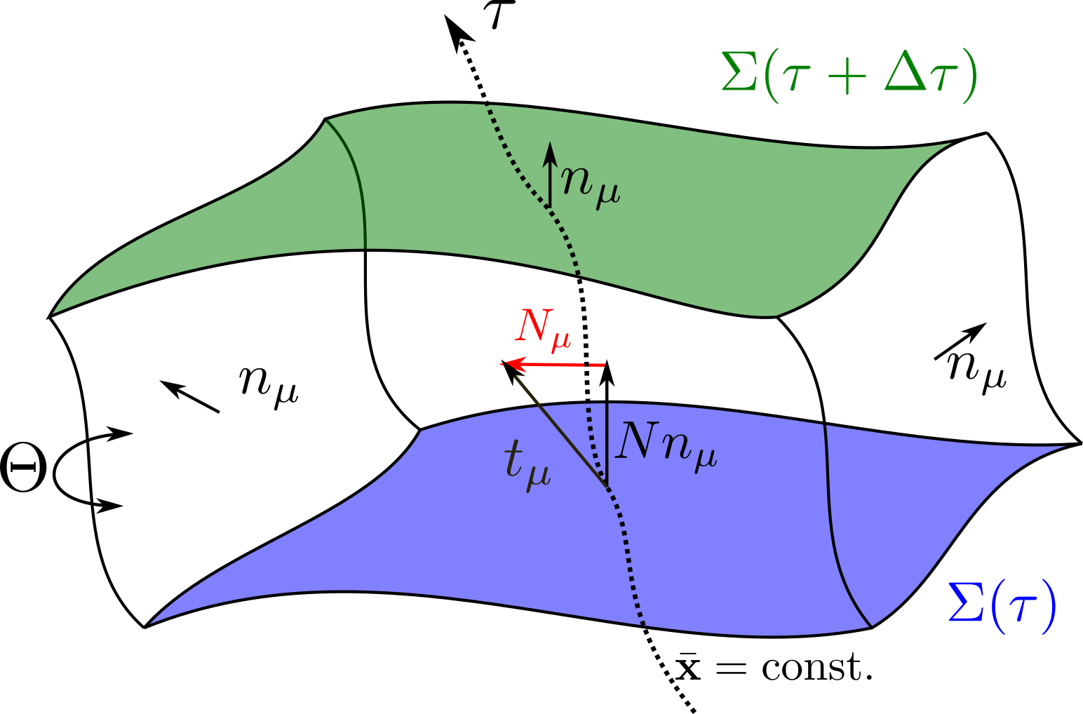
Figure 1.1: The Arnowitt-Deser-Misner (ADM) foliation of the spacetime. $\Sigma(\tau)$ is a space-like hyper-surface parametrized by $\tau(x)=$const. The normal unit vector to hyper-surfaces is denoted by $n^{\mu}$. The figure shows the decomposition of the time vector $t^{\mu}=\partial_{\tau}x^{\mu}=N\,n^{\mu}+N^{\mu}$, with $N(x)$ the lapse function and $N^{\mu}$ the shift vector. The whole region represents the space-time volume $\Omega$ enclosed by two space-like hyper-surface $\Sigma(\tau)$ and $\Sigma(\tau+\Delta\tau)$ and a time-like boundary $\Theta$.

In a relativistic system the symmetries of space-times are dictated by the Poincaré group, which has ten generators. To each generator is associated a conserved quantity. The densities of those conserved quantities are retrieved with a foliation of space-time, slicing it with space-like hyper-surfaces. In a generic curved space-time with metric $g_{\mu\nu}$, we choose a function $\tau(x)$ as a time which parametrize the space-like hyper-surfaces $\Sigma(\tau)$. We indicate with $\bar{\mathchoice{\mbox{\boldmath$\displaystyle\mathbf{x}$}}{\mbox{\boldmath$\textstyle\mathbf{x}$}}{\mbox{\boldmath$\scriptstyle\mathbf{x}$}}{\mbox{\boldmath$\scriptscriptstyle\mathbf{x}$}}}=\bar{\mathchoice{\mbox{\boldmath$\displaystyle\mathbf{x}$}}{\mbox{\boldmath$\textstyle\mathbf{x}$}}{\mbox{\boldmath$\scriptstyle\mathbf{x}$}}{\mbox{\boldmath$\scriptscriptstyle\mathbf{x}$}}}(x)$ the space coordinates on $\Sigma(\tau)$. We can now distinguish two future oriented time-like vectors $n_{\mu}$ and $t_{\mu}$ (see Fig. 1.1). The unit vector normal to the space-like hyper-surfaces is

$$n_{\mu}(x)=N(x)\partial_{\mu}\tau(x)\quad\text{with}\quad N(x)\equiv(\partial^{\mu}\tau(x)\partial_{\mu}\tau(x)))^{-1/2},$$

where $n_{\mu}$ is normalized as $n_{\mu}n^{\mu}=1$ and $N>0$ is the lapse function. $t_{\mu}$ is the local time direction in our coordinate system, which we decompose into the parts perpendicular and parallel to $n_{\mu}$:

$$t^{\mu}(x)\equiv\partial_{\tau}x^{\mu}(\tau,\bar{\mathchoice{\mbox{\boldmath$\displaystyle\mathbf{x}$}}{\mbox{\boldmath$\textstyle\mathbf{x}$}}{\mbox{\boldmath$\scriptstyle\mathbf{x}$}}{\mbox{\boldmath$\scriptscriptstyle\mathbf{x}$}}})=Nn^{\mu}+N^{\mu}\quad\text{with}\quad n_{\mu}N^{\mu}=0,$$

$N^{\mu}$ is called the shift vector. The unit vector $n$ defines the world lines of observer, while $\tau$ in general does not correspond to the proper time of comoving clock. An other significant distinction between the two vectors, is that for Frobenius theorem $n$ must fulfill

$$\epsilon_{\mu\nu\lambda\sigma}n^{\mu}(\partial^{\nu}n^{\lambda}-\partial^{\lambda}n^{\nu})=0$$

meaning that it is irrotational, while, on the contrary, $t$ can posses a vortical distribution.

Denoting with $\mathrm{d}\Sigma(\tau)=N^{-1}\sqrt{-g}\,\mathrm{d}^{d-1}\bar{\mathchoice{\mbox{\boldmath$\displaystyle\mathbf{x}$}}{\mbox{\boldmath$\textstyle\mathbf{x}$}}{\mbox{\boldmath$\scriptstyle\mathbf{x}$}}{\mbox{\boldmath$\scriptscriptstyle\mathbf{x}$}}}$ the volume element on the hyper-surface at constant $\tau(x)$, we define the hyper-surface vector $\mathrm{d}\Sigma_{\mu}=\mathrm{d}\Sigma(\tau)n_{\mu}$. Let $\widehat{j}^{\mu}(x)$ be a conserved current of the system, at a given fixed value of the parametric time $\tau$, the total charge $\widehat{Q}$ is obtained projecting the current along the normal direction $n$ and integrating over all the hyper-surface $\Sigma(\tau)$:

$$\widehat{Q}=\int_{\Sigma(\tau)}\mathrm{d}\Sigma_{\mu}\,\widehat{j}^{\mu}(x).$$

The charge $\widehat{Q}$ do not depend on the specific value of $\tau$, indeed consider the difference of the charge at time $\tau$ and at time $\tau+\Delta\tau$

$$\Delta\widehat{Q}=\int_{\Sigma(\tau+\Delta\tau)}\mathrm{d}\Sigma_{\mu}\,\widehat{j}^{\mu}(x)-\int_{\Sigma(\tau)}\mathrm{d}\Sigma_{\mu}\,\widehat{j}^{\mu}(x).$$

Call $\Omega$ the region enclosed by the two hyper-surfaces $\Sigma(\tau+\Delta\tau)$ and $\Sigma(\tau)$ and call $\Theta$ the time-like hyper-surface that surrounds $\Omega$ (see Fig. 1.1). Then, the difference of charge is the difference between the current flux on the boundary $\partial\Omega$ of the whole region and on the surface $\Theta$:

$$\Delta\widehat{Q}=\int_{\partial\Omega}\mathrm{d}\Sigma_{\mu}\,\widehat{j}^{\mu}(x)-\int_{\Theta}\mathrm{d}\Sigma_{\mu}\,\widehat{j}^{\mu}(x).$$

The second term could be sent to zero by a suitable boundary conditions and the first term can be written by Gauss theorem as the divergence of the current, which is vanishing:

$$\Delta\widehat{Q}=\int_{\Omega}\mathrm{d}\Omega\nabla_{\mu}\,\widehat{j}^{\mu}(x)=0.$$

1.2 Symmetries and conservation laws

Geometry being settled, we are now considering the microscopic description of matter. The most general situation we are dealing in this work is a Dirac field $\psi(x)$ interacting with an external gauge field $A^{\mu}(x)$ in a general curved space-time background $g_{\mu\nu}$. The action related to a particle with spin in curved space-time is not written in terms of the metric, the vierbein vector field $e^{a}_{\,\mu}(x)$ is used instead. It is defined by [33]:

$$g_{\mu\nu}(x)=\eta_{ab}e^{a}_{\,\mu}(x)e^{b}_{\,\nu}(x),\quad e\equiv\det e^{a}_{\,\mu}=\sqrt{-g},$$

where the Greek letters $(\mu,\nu,\dots)$ denote curved space-times indices in the coordinate system $(t,\mathchoice{\mbox{\boldmath$\displaystyle\mathbf{x}$}}{\mbox{\boldmath$\textstyle\mathbf{x}$}}{\mbox{\boldmath$\scriptstyle\mathbf{x}$}}{\mbox{\boldmath$\scriptscriptstyle\mathbf{x}$}})$, while Latin letter $(a,b,\dots)$ denote the local Lorentz indices. The action is then given by the following form

$$S\left[\psi,\bar{\psi};e^{a}_{\,\mu},A_{\mu}\right]=\int\mathrm{d}^{d}x\,e\,\mathcal{L}\left(\psi(x),\bar{\psi}(x),D_{\mu}\psi(x),D_{\mu}\bar{\psi}(x);e^{a}_{\,\mu}(x),A_{\mu}(x)\right)$$ (1.1)

where the covariant derivative acts on the Dirac field as follows:

$$D_{\mu}\psi=\nabla_{\mu}-{\rm i}A_{\mu}=\partial_{\mu}\psi+\frac{1}{2}\omega^{ab}_{\mu}\sigma_{ab}\psi-{\rm i}A_{\mu},$$

where $\sigma_{ab}=\frac{1}{4}[\gamma_{a},\gamma_{b}]$, $\gamma_{a}$ are the flat space time gamma matrices satisfying $\{\gamma^{a},\gamma^{b}\}=2\eta^{ab}$ and $\omega^{ab}_{\mu}$ is the spin connection given by

$$\omega^{ab}_{\mu}=\frac{1}{2}e^{a\nu}(\partial_{\mu}e_{\nu}^{b}-\partial_{\nu}e_{\mu}^{b})-\frac{1}{2}e^{b\nu}(\partial_{\mu}e_{\nu}^{a}-\partial_{\nu}e_{\mu}^{a})+\frac{1}{2}e^{a\nu}e^{b\rho}(\partial_{\rho}e_{\nu}^{c}-\partial_{\nu}e_{\rho}^{c})e_{c\mu}.$$

As a notable examples the Dirac Lagrangian in curved spacetime is written as

$$\mathcal{L}=\frac{{\rm i}}{2}\bar{\psi}\left(\underline{\gamma}^{\mu}\overrightarrow{D}_{\mu}-\overleftarrow{D}_{\mu}\underline{\gamma}^{\mu}\right)\psi-m\bar{\psi}\psi,$$ (1.2)

where we have introduced the coordinate dependent Dirac matrices $\underline{\gamma}^{\mu}(x)\equiv e_{a}^{\,\,\mu}(x)\gamma^{a}$.

Before moving on considering symmetries of the action, once the form of the action is known we can define several quantities that would come in handy. The stress-energy tensor and the electric current are obtained as variation of the action respect to the vierbien and to the guage field respectively:

$$T^{\mu}_{\;a}\equiv\frac{1}{e}\frac{\delta S}{\delta e^{\;a}_{\mu}},\quad J^{\mu}\equiv\frac{1}{e}\frac{\delta S}{\delta A_{\mu}}.$$

The stress-energy tensor with full curved space-times indices is simply derived from the previous one: $T^{\mu}_{\;\nu}\equiv e_{\nu}^{\;a}T^{\mu}_{\;a}$. For the free Dirac field of the Lagrangian (1.2) the stress-energy tensor is

$$T^{\mu\nu}=\frac{1}{4}\left[\bar{\psi}\gamma^{\mu}(D^{\nu}\psi)+\bar{\psi}\gamma^{\nu}(D^{\mu}\psi)-(D^{\nu}\bar{\psi})\gamma^{\mu}\psi-(D^{\mu}\bar{\psi})\gamma^{\nu}\psi\right].$$ (1.3)

Moreover, the field strength tensor of gauge field is defined as $F_{\mu\nu}\equiv\partial_{\mu}A_{\nu}-\partial_{\nu}A_{\mu}$.

Consider first the internal symmetries of the action. We have explicitly chosen the form in Eq. (1.1) with a gauged covariant derivative such that the action posses gauge invariance under the U(1) transformation related to the field $A_{\mu}$. Upon a transformation with an infinitesimal parameter $\alpha(x)$, assumed to be vanishing on the boundary, the fields change into

$$\delta_{\alpha}A_{\mu}=\partial_{\mu}\alpha,\quad\delta_{\alpha}\psi={\rm i}q\alpha\psi,\quad\delta_{\alpha}\bar{\psi}=-{\rm i}q\alpha\bar{\psi}$$

with $q=\pm 1$ or $0$ the elementary charge of Dirac field. The variation of the action respect to this transformation is vanishing because we supposed it invariant. However, we could explicitly write the form of the variation. Dirac field gives a contribution proportional to the equations of motions $\delta S/\delta\psi=0$ and $\delta S/\delta\bar{\psi}=0$, therefore the action variation is written as

$$\begin{split}\delta_{\alpha}S=&\int\mathrm{d}^{d}x\,e\,J^{\mu}\delta_{\alpha}A_{\mu}=\int\mathrm{d}^{d}x\,e\,J^{\mu}\partial_{\mu}\alpha\\ =&\int\mathrm{d}^{d}x\,e\nabla_{\mu}\left(J^{\mu}\alpha\right)-\int\mathrm{d}^{d}x\,e\,\alpha\,\nabla_{\mu}J^{\mu}.\end{split}$$

The first term vanishes because $\alpha$ is vanishing on the boundary and since the action variation is zero for any function $\alpha$, this implies that the current $J^{\mu}$ must be a conserved current:

$$\nabla_{\mu}J^{\mu}=0.$$ (1.4)

The action may posses several internal symmetries, for instance related to electric or baryon charge conservation. One peculiar case of such charges is chiral charge, also called axial charge. In the case of massless field ($m=0$) the Dirac Lagrangian (1.2) is invariant under the unitary “chiral” transformation defined by:

$$\psi\to\psi^{\prime}=\mathrm{e}^{{\rm i}\alpha\gamma^{5}}\psi,$$

where $\gamma^{5}$ is obtained from flatspace gamma matrices $\gamma^{5}={\rm i}\gamma^{0}\gamma^{1}\gamma^{2}\gamma^{3}$. This correspond to the infinitesimal change of the fields:

$$\delta_{\alpha}\psi={\rm i}\alpha\gamma^{5}\psi,\quad\delta_{\alpha}\bar{\psi}={\rm i}\alpha\bar{\psi}\gamma^{5}.$$

The explicit variation of the action with Lagrangian (1.2) is

$$\delta_{\alpha}S=-\int\mathrm{d}^{d}x\,e\left[\left(\bar{\psi}\underline{\gamma}^{\mu}\gamma^{5}\psi\right)\partial_{\mu}\alpha+2{\rm i}m\bar{\psi}\gamma^{5}\psi\,\alpha\right],$$

which upon part integration of the $\partial_{\mu}\alpha$ term gives the conservation equation

$$\nabla_{\mu}J_{\textup{A}}^{\mu}=2{\rm i}m\bar{\psi}\gamma^{5}\psi,$$ (1.5)

where we defined

$$J_{\textup{A}}^{\mu}\equiv\bar{\psi}\underline{\gamma}^{\mu}\gamma^{5}\psi$$ (1.6)

the axial (or chiral) current. The relation (1.5) can also be obtained from equation of motions starting from the current definition (1.6). What is special about axial current is that, contrary to electric current, the conservation equation holds only at classical level and may be altered when quantum processes are considered. When fermions interacts with some gauge fields [19] or in presence of space-time curvature [34], quantum processes generate axial current and the net charge is not conserved. The current is said to be anomalous and, in $d=4$ dimensions, the axial current divergence is

$$\nabla_{\mu}J^{\mu}_{\textup{A}}=2{\rm i}m\bar{\psi}\gamma^{5}\psi-\frac{1}{8}\epsilon^{\mu\nu\lambda\sigma}\frac{q^{2}}{2\pi^{2}}F_{\mu\nu}F_{\lambda\sigma}+\frac{1}{8}\epsilon^{\mu\nu\lambda\sigma}\frac{1}{48\pi^{2}}R^{\alpha}_{\,\beta\mu\nu}R^{\beta}_{\,\alpha\lambda\sigma}.$$ (1.7)

In this work, we mostly consider Dirac fermions with zero mass and in flat space-time, therefore the only source of axial non conservation can only come from gauge fields. When gauge fields are external electromagnetic field, there exist configurations of electric and magnetic fields such that the second term in Eq. (1.7) is vanishing and the chiral charge is indeed conserved. Replacing the definitions of strength tensor and of electric $E$ and magnetic $B$ field, we find that term is written as

$$\frac{1}{2}\epsilon^{\mu\nu\lambda\sigma}F_{\mu\nu}F_{\lambda\sigma}=4B\cdot E.$$

We therefore see that this term is vanishing when the electric and magnetic fields are orthogonal one to an other or simply when one of the two is vanishing. If, on the other hand, this term is not vanishing or we are dealing with dynamical gauge fields, the right hand side of Eq. (1.7) at zero mass can be written as the divergence of the so-called Chern-Simons current [35]:

$$\begin{split}K^{\mu}=&\frac{q^{2}}{8\pi^{2}}\epsilon^{\mu\nu\rho\sigma}A_{\nu}F_{\rho\sigma}-\frac{1}{8}\epsilon^{\mu\nu\rho\lambda}\frac{1}{48\pi^{2}}\Gamma^{\alpha}_{\,\nu\beta}\left(\partial_{\rho}\Gamma^{\beta}_{\alpha\lambda}+\frac{2}{3}\Gamma^{\beta}_{\,\rho\sigma}\Gamma^{\sigma}_{\,\alpha\lambda}\right),\\ \nabla^{\mu}K_{\mu}=&\frac{1}{8}\epsilon^{\mu\nu\lambda\sigma}\frac{q^{2}}{2\pi^{2}}F_{\mu\nu}F_{\lambda\sigma}-\frac{1}{8}\epsilon^{\mu\nu\lambda\sigma}\frac{1}{48\pi^{2}}R^{\alpha}_{\,\beta\mu\nu}R^{\beta}_{\,\alpha\lambda\sigma}\end{split}$$

where $\Gamma$’s are the Christoffel symbols and the integral of Chern-Simons current can be embodied in the definition of a gauge-invariant overall conserved axial charge including both fermion and gauge contribution:

$$J^{\mu}_{\textup{CS}}=J^{\mu}_{\textup{A}}+K^{\mu},\quad\partial_{\mu}J^{\mu}_{\textup{CS}}=0.$$

Moving to other symmetries, we also want our action to be compatible with relativity principles, therefore we ask that our description is unaffected by the local inertial frame chosen. The action is then invariant under Lorentz transformations:

$$\delta_{\Omega}\,e^{\;a}_{\mu}=\Omega^{a}_{\;b}(x)e^{\;b}_{\mu},\quad\delta_{\Omega}\psi=-\frac{{\rm i}}{2}\Omega^{ab}(x)\Sigma_{ab}\psi,\quad\delta_{\Omega}\bar{\psi}=\frac{{\rm i}}{2}\Omega^{ab}(x)\bar{\psi}\Sigma_{ab},$$

where $\Omega_{ab}=-\Omega_{ba}$ denotes an infinitesimal local rotation angle and $\Sigma_{ab}$ are the generators of Lorentz group. Again, taking advantage of the Eq.s of motions, the action variation is given by

$$\begin{split}\delta_{\Omega}\,S=&\int\mathrm{d}^{d}x\,e\,T^{\mu}_{\;a}\,\,\delta_{\Omega}\,e^{\;a}_{\mu}=-\int\mathrm{d}^{d}x\,e\,T^{ab}\Omega_{ab}\\ =&-\int\mathrm{d}^{d}x\,e\frac{1}{2}\left(T^{ab}-T^{ba}\right)\Omega_{ab}.\end{split}$$

Therefore, Lorentz invariance requires that the stress-energy-tensor is symmetric under the exchange of local Lorentz indices:

$$T^{ab}-T^{ba}=0.$$ (1.8)

At last, the action must be invariant under diffeomorphism transformations. Consider then the general infinitesimal coordinate transformation

$$x^{\mu}\to x^{\prime\mu}=x^{\mu}-\xi^{\mu}(x)$$

where $\xi$ is chosen such that it is vanishing on the boundary region. Under this transformation, the variation of the fields are given by the Lie derivative along $\xi^{\mu}$

$$\mathcal{L}_{\xi}e^{a}_{\,\mu}\equiv e^{\prime a}_{\,\mu}(x)-e^{a}_{\,\mu}(x)=\xi^{\nu}\nabla_{\nu}e^{a}_{\,\mu}+e^{a}_{\,\nu}\nabla_{\mu}\xi^{\nu}$$

$$\mathcal{L}_{\xi}A_{\mu}\equiv A^{\prime}_{\mu}(x)-A_{\mu}(x)=\xi^{\nu}\nabla_{\nu}A_{\mu}+A_{\nu}\nabla_{\mu}\xi^{\nu}$$

$$\mathcal{L}_{\xi}\psi\equiv\psi^{\prime}(x)-\psi(x)=\xi^{\nu}\partial_{\nu}\psi$$

$$\mathcal{L}_{\xi}\bar{\psi}\equiv\bar{\psi}^{\prime}(x)-\bar{\psi}(x)=\xi^{\nu}\partial_{\nu}\bar{\psi}.$$

Consequently, the action transforms as follows

$$\begin{split}\delta_{\xi}S=&\int\mathrm{d}^{d}x\,e\left[T^{\mu}_{\;a}\mathcal{L}_{\xi}e^{\;a}_{\mu}+J^{\mu}\mathcal{L}_{\xi}A_{\mu}\right]\\ =&\int\mathrm{d}^{d}x\,e\left[T^{\mu}_{\;a}\left(\xi^{\nu}\nabla_{\nu}e^{\;a}_{\mu}+e^{\;a}_{\nu}\nabla_{\mu}\xi^{\nu}\right)+J^{\mu}\left(\xi^{\nu}\nabla_{\nu}A_{\mu}+A_{\nu}\nabla_{\mu}\xi^{\nu}\right)\right]\\ =&-\int\mathrm{d}^{d}x\,e\left[\left(\nabla_{\mu}T^{\mu}_{\;\nu}-F_{\nu\lambda}J^{\lambda}\right)\xi^{\nu}\right]+\int\mathrm{d}^{d}x\,e\,T_{ab}\,\omega^{ab}_{\nu}\,\xi^{\nu}\\ &+\int\mathrm{d}^{d}x\,e\nabla_{\mu}\left[\left(T^{\mu}_{\;\nu}+J^{\mu}A_{\nu}\right)\xi^{\nu}\right]-\int\mathrm{d}^{d}x\,e\,\xi^{\nu}A_{\nu}\nabla_{\mu}J^{\mu},\end{split}$$

where we used the identity [33]

$$D_{\mu}e^{\;a}_{\nu}=\nabla_{\mu}e^{\;a}_{\nu}+\omega^{\;a}_{\mu\;b}e^{\;b}_{\nu}=0.$$

The last term in the action variation vanishes because $J$ is a conserved current, the third term because $\xi$ is vanishing on the boundary and the second term because the stress-energy tensor is symmetric, while spin-connection is anti-symmetric. Therefore, diffeomorphism invariance impose the following conservation Eq.s for the stress-energy tensor:

$$\nabla_{\mu}T^{\mu}_{\;\nu}=F_{\nu\lambda}J^{\lambda}.$$ (1.9)

If $J$ is an electric current, then $F_{\nu\lambda}J^{\lambda}$ is the external Lorentz force which drives the energy and the momentum of the system. It is trivial to notice that in absence of external gauge (force) the stress-energy tensor is conserved.

1.3 Local equilibrium

In the previous sections we provided a space-time foliation in order to access local covariant quantities and we derived the conserved quantities related to the invariance of coordinate, Lorentz and U(1) transformations. We can now proceed to define the covariant local equilibrium density operator.

Choose a foliation of space-time and suppose that the system in consideration thermalize faster than the evolution of “time” $\tau$ in which we are interested. Then, at each step of evolution $\mathrm{d}\tau$, the system is at local thermal equilibrium and the macroscopic behavior of the system is described by a stress-energy density $T_{\mu\nu}(x)$ and a current density $j_{\mu}(x)$ lying on the space-like hyper-surface $\Sigma(\tau)$. Now, we want to describe the system based on the density operator which lives on $\Sigma(\tau)$. As in the non-relativistic case, the local density operator at local equilibrium $\widehat{\rho}_{\textup{LE}}$ is defined as the operator which maximizes the entropy $S=-{\text{tr}}(\widehat{\rho}\log\widehat{\rho})$. As for the constraints, since we want to reproduce the thermodynamics on the hyper-surface, we impose that the mean values of the stress-energy tensor and of the current on $\Sigma(\tau)$ corresponds to the actual values of the densities $T_{\mu\nu}(x)$ and $j_{\mu}(x)$. To obtain these densities, we project the stress–energy tensor and the current mean values onto the normalized vector perpendicular to $\Sigma$:

$$\begin{split}n_{\mu}(x){\text{tr}}(\widehat{\rho}\,\,\widehat{T}^{\mu\nu}(x))=&\,n_{\mu}(x)\langle\widehat{T}^{\mu\nu}(x)\rangle\equiv n_{\mu}(x)T^{\mu\nu}(x),\\ n_{\mu}(x){\text{tr}}(\widehat{\rho}\,\,\widehat{j}^{\mu}(x))=&\,n_{\mu}(x)\langle\widehat{j}^{\mu}(x)\rangle\equiv n_{\mu}(x)j^{\mu}(x).\end{split}$$ (1.10)

In addition to the energy, momentum, and charge densities, one should include the angular momentum density, but if the stress–energy tensor is the Belinfante, this further constraint is redundant and can be disregarded [36]. Therefore, from now on, the stress-energy tensor is considered to be symmetric.

At any fixed $\tau$, the maximization of entropy is obtained introducing the Lagrange multiplier functions $\beta^{\nu}(x)$ and $\zeta(x)$ and finding the extreme with respect to $\widehat{\rho}$ for the functional $F$:

$$\begin{split}F[\,\widehat{\rho}\,]=&-{\text{tr}}\left(\,\widehat{\rho}\log\widehat{\rho}\,\right)+\\ &+\int_{\Sigma(\tau)}\mathrm{d}\Sigma\;n_{\mu}(x)\left[\left(\langle\widehat{T}^{\mu\nu}(x)\rangle-T^{\mu\nu}(x)\right)\beta_{\nu}(x)-\left(\langle\widehat{j}^{\mu}(x)\rangle-j^{\mu}(x)\right)\zeta(x)\right].\end{split}$$

The maximum solution $\widehat{\rho}_{\textup{LE}}$ gives the Local Equilibrium Density Operator (LEDO) [26, 31]:

$$\widehat{\rho}_{\textup{LE}}=\dfrac{1}{\mathcal{Z}_{\textup{LE}}}\exp\left[-\int_{\Sigma(\tau)}\mathrm{d}\Sigma\;n_{\mu}(x)\left(\widehat{T}^{\mu\nu}(x)\beta_{\nu}(x)-\widehat{j}^{\mu}(x)\zeta(x)\right)\right],$$ (1.11)

where $\mathcal{Z}_{\textup{LE}}$ is chosen such that the density operator is normalized, i.e. ${\text{tr}}(\,\widehat{\rho}_{\textup{LE}})=1$. The physical meaning of the four-vector $\beta$ and the scalar $\zeta$ are respectively those of the temperature four-vector and the ratio between local chemical potential and temperature. They are obtained as solution of the constraints (1.10) with $\widehat{\rho}=\widehat{\rho}_{\textup{LE}}$:

$$n_{\mu}(x)T^{\mu\nu}_{\textup{LE}}[\beta,\zeta,n]=n_{\mu}(x)T^{\mu\nu}(x),\quad n_{\mu}(x)j^{\mu}_{\textup{LE}}[\beta,\zeta,n]=n_{\mu}(x)j^{\mu}(x).$$

These equations identify a time-like four-vector $\beta$ which in turn can be used as hydrodynamic frame by choosing the unitary fluid four-velocity $u$ as

$$u=\frac{\beta}{\sqrt{\beta^{2}}}=T\beta,$$

referred as $\beta$-frame [26] or thermodynamic frame [37].

It should be noted that $\widehat{\rho}_{\textup{LE}}$ is not the true density operator. Indeed, the true density operator in Heisenberg picture is time-independent, while the operator in Eq. (1.11) is explicitly dependent on time through the time dependence of the operators. The true density operator can be derived from $\widehat{\rho}_{\textup{LE}}$ assuming that at a certain time $\tau_{0}$ the system is at local thermal equilibrium. This means that at that particular time the true density operator coincides with the LEDO. Then the true statistical operator is obtained evolving the system in $\tau$ [26, 29].

We are instead interested in the system when it reaches the global thermal equilibrium. This is obtained when the LEDO is time-independent and do not depend on the parametrization chosen for the foliation.

1.4 General global equilibrium

We want to make the LEDO (1.11) independent of time parametrization and consequently stationary. There exist peculiar configurations of the $\beta$ and $\zeta$ fields which make the exponent of Eq. (1.11) divergent free [38]. As we are now proving, this is sufficient to keep the statistical operator independent of the foliation.

Choose any foliation and consider two space-like hyper-surfaces at different time: $\Sigma(\tau)$ and $\Sigma(\tau+\Delta\tau)$. As in figure 1.1, we call $\Omega$ the region of space-time enclosed by those hyper-surfaces and by $\Theta$ the time-like part of the boundary $\partial\Omega$. We integrate the four-divergence of the local operator in the exponent of the LEDO (1.11) over the region $\Omega$; the integral can be turned by Gauss theorem into the flux through the boundary:

$$\int_{\Omega}\mathrm{d}\Omega\;\nabla_{\mu}\left(\widehat{T}^{\mu\nu}(x)\beta_{\nu}(x)-\widehat{j}^{\mu}(x)\zeta(x)\right)=\int_{\partial\Omega}\mathrm{d}\Sigma_{\mu}\left(\widehat{T}^{\mu\nu}(x)\beta_{\nu}(x)-\widehat{j}^{\mu}(x)\zeta(x)\right).$$

The whole flux can be decomposed into the sum of the single fluxes over each boundary surface of region $\Omega$:

$$\begin{split}\int_{\partial\Omega}&\mathrm{d}\Sigma_{\mu}\left(\widehat{T}^{\mu\nu}(x)\beta_{\nu}(x)-\widehat{j}^{\mu}(x)\zeta(x)\right)=\int_{\Theta}\mathrm{d}\Sigma_{\mu}\left(\widehat{T}^{\mu\nu}(x)\beta_{\nu}(x)-\widehat{j}^{\mu}(x)\zeta(x)\right)\\ &+\int_{\Sigma(\tau+\Delta\tau)}\!\!\!\!\mathrm{d}\Sigma_{\mu}\left(\widehat{T}^{\mu\nu}(x)\beta_{\nu}(x)-\widehat{j}^{\mu}(x)\zeta(x)\right)-\int_{\Sigma(\tau)}\!\!\mathrm{d}\Sigma_{\mu}\left(\widehat{T}^{\mu\nu}(x)\beta_{\nu}(x)-\widehat{j}^{\mu}(x)\zeta(x)\right).\end{split}$$

The first term is vanishing for a suitable boundary condition of the fields $\beta$ and $\zeta$. As found in section 1.1 for a charge of a system, the shift by time evolution of the local operator in the exponent is given by the integral of a divergence:

$$\begin{split}\int_{\Omega}&\mathrm{d}\Omega\;\nabla_{\mu}\left(\widehat{T}^{\mu\nu}(x)\beta_{\nu}(x)-\widehat{j}^{\mu}(x)\zeta(x)\right)=+\int_{\Sigma(\tau+\Delta\tau)}\mathrm{d}\Sigma_{\mu}\left(\widehat{T}^{\mu\nu}(x)\beta_{\nu}(x)-\widehat{j}^{\mu}(x)\zeta(x)\right)\\ &-\int_{\Sigma(\tau)}\mathrm{d}\Sigma_{\mu}\left(\widehat{T}^{\mu\nu}(x)\beta_{\nu}(x)-\widehat{j}^{\mu}(x)\zeta(x)\right).\end{split}$$

It follows that the vanishing of the integrand on the l.h.s is a sufficient condition for the exponent of the LEDO to be time independent. Once it is time independent, it does not matter at which time $\tau$ are evaluating your local operator and by extensions it does not matter which time functions $\tau(x)$ you picked for space-time foliation. In other words, it is also independent on the foliation chosen.

The specific configurations of the $\beta$ and $\zeta$ fields that make the four-divergence vanishing are obtained taking advantage of the conservation equation of stress-energy tensor (1.9) and current (1.4). In the following derivation, we are also including a conserved axial current $\widehat{j}_{\textup{A}}$ with a corresponding Lagrange multiplier $\zeta_{\textup{A}}(x)$. As discussed in Sec. 1.2, for a massless Dirac field, even in the presence of anomalies, we can always define a conserved current $\widehat{j}_{\textup{CS}}$ related to chiralty by means of Chern-Simons current. Therefore, when we are considering massless fermions affected by external or dynamic gauge fields, we always implicitly refer to global equilibrium with chiral imbalance related to conserved current $\widehat{j}_{\textup{CS}}$. In the case of massive field, or more generally when a conserved axial current can not be defined, global thermal equilibrium with a non-vanishing Lagrange multiplier can not be reached because the axial current will make the statistical operator dependent on time. In that case, we can simply set $\zeta_{\textup{A}}=0$ so that the following expressions and arguments remain valid. To enforce a vanishing four-divergence the $\beta$, $\zeta$ and $\zeta_{\textup{A}}$ field must satisfy

$$\begin{split}0=&\nabla_{\mu}\left(\widehat{T}^{\mu\nu}(x)\beta_{\nu}(x)-\widehat{j}^{\mu}(x)\zeta(x)-\widehat{j}_{\textup{A}}^{\mu}(x)\zeta_{\textup{A}}(x)\right)\\ =&\beta_{\nu}(x)\nabla_{\mu}\widehat{T}^{\mu\nu}(x)+\widehat{T}^{\mu\nu}(x)\nabla_{\mu}\beta_{\nu}(x)\\ &-\widehat{j}^{\mu}(x)\nabla_{\mu}\zeta(x)-\zeta(x)\,\nabla_{\mu}\widehat{j}^{\mu}(x)-\widehat{j}_{\textup{A}}^{\mu}(x)\nabla_{\mu}\zeta_{\textup{A}}(x)-\zeta_{\textup{A}}(x)\,\nabla_{\mu}\widehat{j}_{\textup{A}}^{\mu}(x)\\ =&\widehat{T}^{\mu\nu}(x)\nabla_{\mu}\beta_{\nu}(x)-\left[\nabla^{\mu}\zeta(x)-F^{\nu\mu}(x)\beta_{\nu}(x)\right]\widehat{j}_{\mu}(x)-\nabla_{\mu}\zeta_{\textup{A}}(x)\widehat{j}^{\mu}_{\textup{A}}(x)=0\end{split}$$

Then, using the fact that stress-energy tensor is symmetric, we see that the previous quantity is vanishing if the $\beta$, $\zeta$ and $\zeta_{\textup{A}}$ fields satisfy:

$$\nabla_{\mu}\beta_{\nu}(x)+\nabla_{\nu}\beta_{\mu}(x)=0,\qquad\nabla^{\mu}\zeta(x)=F^{\nu\mu}(x)\beta_{\nu}(x),\qquad\nabla^{\mu}\zeta_{\textup{A}}(x)=0.$$

The first equation impose that $\beta$ is a Killing vector field. The second equation has a simple physical interpretation. In the beta frame, the fluid velocity $u$ is the unit four vector directed along the four inverse-temperature $\beta$. Starting from that time-like vector we can define the comoving electric and magnetic fields:

$$E^{\mu}=F^{\mu\lambda}u_{\lambda},\quad B^{\mu}=\frac{1}{2}\epsilon^{\mu\nu\rho\sigma}F_{\nu\rho}u_{\sigma};\quad F^{\mu\nu}=E^{\mu}u^{\nu}-E^{\nu}u^{\mu}-\epsilon^{\mu\nu\rho\sigma}B_{\rho}u_{\sigma}.$$ (1.12)

Indicating with $T(x)$ the temperature $1/T(x)=\sqrt{\beta^{2}(x)}$, the second condition can be written as

$$T(x)\nabla^{\mu}\left(\frac{\mu(x)}{T(x)}\right)-E^{\mu}(x)=0,$$

meaning that a system subject to an external electric field will develop a gradient of $\mu/T$ in order to compensate the applied field and ensure that the equilibrium is maintained. It is also worth noticing that even in presence of a comoving magnetic field if the comoving electric field is vanishing, equilibrium is reached only with a constant $\zeta$ filed. The condition on $\zeta_{\textup{A}}$ simply states that the ratio between chiral chemical potential and temperature $\zeta_{\textup{A}}=\mu_{\textup{A}}(x)/T(x)$ must be constant.

In flat space-time, the general solution for the Killing equation $\partial_{\mu}\beta_{\nu}+\partial_{\mu}\beta_{\mu}=0$ is given in terms of a constant vector $b_{\nu}$ and a constant anti-symmetric tensor $\varpi_{\mu\nu}$:

$$\beta_{\mu}(x)=b_{\mu}+\varpi_{\mu\nu}x^{\nu}.$$ (1.13)

The anti-symmetric tensor $\varpi_{\mu\nu}$ is dubbed thermal vorticity and can be expressed by means of Eq. (1.13) as an exterior derivative of the $\beta$ field:

$$\varpi_{\mu\nu}=-\frac{1}{2}\left(\partial_{\mu}\beta_{\nu}-\partial_{\nu}\beta_{\mu}\right).$$

Since in this chapter we are introducing global equilibrium with vorticity, in order to not overburden the chapter, we now deal with a vanishing electromagnetic field. The global equilibrium with both vorticity and external electromagnetic field is discussed in Sec. 4.3. Consider then a system without an external gauge field. In this case, at global equilibrium the $\zeta$ field must be a constant. Inserting the configurations (1.13), $\zeta=$const. and $\zeta_{\textup{A}}=$const. into the LEDO (1.11), we find the general global equilibrium density operator:

$$\widehat{\rho}_{\textup{GE}}=\dfrac{1}{\mathcal{Z}_{\textup{GE}}}\exp\left[-\int_{\Sigma(\tau)}\mathrm{d}\Sigma\;n_{\mu}(x)\left(\widehat{T}^{\mu\nu}(x)\left(b_{\nu}+\varpi_{\nu\rho}x^{\rho}\right)-\widehat{j}^{\mu}(x)\zeta-\widehat{j}_{\textup{A}}^{\mu}(x)\zeta_{\textup{A}}\right)\right].$$

The quantities $b$, $\varpi$, $\zeta$ and $\zeta_{\textup{A}}$ are constant and can be taken outside the integral. The integration in the exponential reproduce the Poincaré generators, which are conserved quantities. The term linear in $b$ reproduces the four-momentum of the system which is the generator of translation and is given by:

$$\widehat{P}^{\nu}=\displaystyle\int_{\Sigma(\tau)}\mathrm{d}\Sigma_{\mu}(x)\widehat{T}^{\mu\nu}(x).$$

Using the antisymmetry of $\varpi$, the term in vorticity is written as

$$\widehat{T}^{\mu\nu}\varpi_{\nu\rho}x^{\rho}=\frac{1}{2}\left(\widehat{T}^{\mu\nu}x^{\rho}-\widehat{T}^{\mu\rho}x^{\nu}\right)\varpi_{\nu\rho}$$

and upon integration, it reproduces the Lorentz generators:

$$\widehat{J}^{\mu\nu}=\int_{\Sigma}\mathrm{d}\Sigma_{\lambda}(x^{\mu}\widehat{T}^{\lambda\nu}-x^{\nu}\widehat{T}^{\lambda\mu}).$$ (1.14)

The term proportional to $\zeta$ ($\zeta_{\textup{A}}$) gives the electric (axial) charge:

$$\widehat{Q}=\int_{\Sigma(\tau)}\mathrm{d}\Sigma_{\mu}(x)\widehat{j}^{\mu}(x),\quad\widehat{Q}_{\textup{A}}=\int_{\Sigma(\tau)}\mathrm{d}\Sigma_{\mu}(x)\widehat{j}_{\textup{A}}^{\mu}(x).$$ (1.15)

The whole global equilibrium density operator is therefore written in terms of conserved quantities of the system:

$$\widehat{\rho}_{\textup{GE}}=\dfrac{1}{\mathcal{Z}_{\textup{GE}}}\exp\left[-b_{\mu}\widehat{P}^{\mu}+\frac{1}{2}\varpi:\widehat{J}+\zeta\widehat{Q}+\zeta_{\textup{A}}\widehat{Q}_{\textup{A}}\right].$$ (1.16)

This general global equilibrium can be regarded both as a local equilibrium with a specific local temperature $\beta(x)$ or as a true global equilibrium with time independent entropy. Excluding the parameters $\zeta$ and $\zeta_{\textup{A}}$ which correspond to internal symmetries, the density operator depends on 10 parameters, corresponding to the 4 components of $b_{\mu}$ and the 6 independent components of the anti-symmetric tensor $\varpi_{\mu\nu}$. This is the maximum number of first integrals for a relativistic system, each one corresponding to a generator of the Poincaré group.

Given a fixed point in space-time $x$, we can write the general equilibrium density operator in terms of the inverse temperature evaluated at that point. First, taking advantage of Poincaré algebra identities [39], we evaluate the angular momentum operator at $x$ by using the translational operator $\widehat{\sf T}(x)=\exp[\,{\rm i}x\cdot\widehat{P}\,]$:

$$\begin{split}\widehat{J}^{\mu\nu}_{x}\equiv&\widehat{\sf T}(x)\widehat{J}^{\mu\nu}\widehat{\sf T}^{-1}(x)=\widehat{J}^{\mu\nu}-x^{\mu}\widehat{P}^{\nu}+x^{\nu}\widehat{P}^{\mu}\\ &=\int_{\Sigma}\mathrm{d}\Sigma_{\lambda}\left[(y^{\mu}-x^{\mu})\widehat{T}^{\lambda\nu}(y)-(y^{\nu}-x^{\nu})\widehat{T}^{\lambda\mu}(y)\right].\end{split}$$ (1.17)

With this definition and writing $b$ in terms of $\beta(x)$ thanks to Eq. (1.13), the density matrix takes the form

$$\widehat{\rho}_{\textup{GE}}=\dfrac{1}{\mathcal{Z}_{\textup{GE}}}\exp\left[-\beta_{\mu}(x)\widehat{P}^{\mu}+\frac{1}{2}\varpi:\widehat{J}_{x}+\zeta\widehat{Q}+\zeta_{\textup{A}}\widehat{Q}_{\textup{A}}\right].$$ (1.18)

This form will be useful for evaluating mean values of observables around the point in $x$ as a perturbative expansion in thermal vorticity.

The statistical operator (1.16) describes a stationary global equilibrium that in presence of vorticity and it is not homogeneous. Indeed, the four-temperature $\beta$ in Eq. (1.13) depends linearly on the coordinate $x$. However for a vanishing thermal vorticity $\varpi$ the inverse temperature is a constant $\beta=b$ and the usual homogeneous global thermal equilibrium is recovered:

$$\widehat{\rho}=\dfrac{1}{\mathcal{Z}}\exp\left[-\beta_{\mu}\widehat{P}^{\mu}+\zeta\widehat{Q}+\zeta_{\textup{A}}\widehat{Q}_{\textup{A}}\right].$$

Moreover, specializing the thermal vorticity into the values $b_{\mu}=(1/T,\mathbf{0})$ and $\varpi_{\mu\nu}=\omega/T(\delta^{1}_{\mu}\delta^{2}_{\nu}-\delta^{2}_{\mu}\delta^{1}_{\nu})$ we recover the covariant form of the statistical operator used for rotating systems in [40]:

$$\widehat{\rho}_{\omega}=\dfrac{1}{\mathcal{Z}_{\omega}}\exp\left(-\widehat{H}/T+\omega\widehat{J}_{z}/T+\mu\widehat{Q}/T\right),$$

where $\widehat{J}_{z}$ is the angular momentum of the system along the $z$ axis. This operator has been used to address quantum effects in relativistic matter under rotation [41, 42]. Similarly, indicating with $\widehat{K}_{z}$ the generator of a Lorentz boost along the $z$ axis, the parameter choice

$$b_{\mu}=(1/T,0,0,0),\quad\varpi_{\mu\nu}=(a/T)(g_{0\mu}g_{3\nu}-g_{3\mu}g_{0\nu})$$

reproduces an ensemble representing the equilibrium of a relativistic fluid with constant comoving acceleration $a$ along the $z$ direction [43]:

$$\widehat{\rho}_{a}=\frac{1}{\mathcal{Z}_{a}}\exp\left(-\widehat{H}/T+a\widehat{K}_{z}/T\right).$$

1.5 Thermal vorticity and Lie transported basis

Here we show that the anti-symmetric tensor $\varpi$, coming from the Killing solution of inverse temperature, has indeed the physical meaning of fluid acceleration and rotation. If the $\beta$ four-vector (1.13) is a time-like vector, then we can choose the $\beta$-frame as hydrodynamic frame [38, 44]. The unitary four-vector fluid velocity $u$ is therefore identified with the direction of $\beta$:

$$u^{\mu}(x)=\frac{\beta^{\mu}(x)}{\sqrt{\beta_{\rho}(x)\beta^{\rho}(x)}}.$$

As long as we are considering physical observables in a region where the coordinate $x$ are such that $\beta(x)$ is a time-like vector, this choice is perfectly legit and free of issues.

We can decompose the thermal vorticity into two space-like vector fields, each having three independent components, by projecting along the time-like fluid velocity $u$. This is analogous to the decomposition of the also anti-symmetric electromagnetic strength tensor $F$ into an electric and magnetic part. For the thermal vorticity $\varpi$, the decomposition

$$\varpi^{\mu\nu}=\epsilon^{\mu\nu\rho\sigma}w_{\rho}u_{\sigma}+\alpha^{\mu}u^{\nu}-\alpha^{\nu}u^{\mu}$$

defines the four-vectors $\alpha$ and $w$ which are explicitly written inverting the previous relation:

$$\alpha^{\mu}(x)\equiv\varpi^{\mu\nu}u_{\nu},\quad w^{\mu}(x)\equiv-\frac{1}{2}\epsilon^{\mu\nu\rho\sigma}\varpi_{\nu\rho}u_{\sigma}.$$ (1.19)

Notice that $w$ has a minus sign compared to comoving magnetic field in Eq. (1.12). The vectors $\alpha$ and $w$ depends on the coordinate and are space-like and orthogonal to $u$. All the quantity $u,\,\varpi,\,\alpha,\,w$ are dimensionless. A physical interpretation is easily assigned to the vectors $\alpha$ and $w$ if we express them as derivative of the fluid velocity.

First, notice that, at global equilibrium, the thermal vorticity is just the derivative of $\beta$ four-vector: $\varpi_{\mu\nu}=\partial_{\nu}\beta_{\mu}$. Then, it easily realized that comoving temperature along the flow lines does not changes:

$$u_{\nu}\partial^{\nu}\sqrt{\beta^{2}}=\frac{u_{\nu}\beta^{\rho}\partial^{\nu}\beta_{\rho}}{\sqrt{\beta^{2}}}=\frac{u_{\nu}\beta^{\rho}\varpi^{\nu}_{\rho}}{\sqrt{\beta^{2}}}=u^{\rho}\alpha_{\rho}=0.$$

The $\alpha$ vector is then written as

$$\begin{split}\alpha^{\mu}=&\varpi^{\mu\nu}u_{\nu}=u_{\nu}\partial^{\nu}\beta^{\mu}=u^{\mu}u_{\nu}\partial^{\nu}\sqrt{\beta^{2}}+\sqrt{\beta^{2}}u_{\nu}\partial^{\nu}u^{\mu}\\ =&\sqrt{\beta^{2}}u_{\nu}\partial^{\nu}u^{\mu}=\frac{1}{T}a^{\mu},\end{split}$$

where $T=1/\sqrt{\beta^{2}}$ is the proper temperature and $a^{\mu}=u_{\nu}\partial^{\nu}u^{\mu}$ is the acceleration field of the fluid. Therefore, the vector $\alpha$ is the local acceleration of the fluid divided by the temperature. The four-vector $w$ is instead expressed as the local rotation of the fluid $\omega$, sometimes called local vorticity,

$$\omega^{\mu}\equiv\frac{1}{2}\epsilon^{\mu\nu\rho\sigma}u_{\sigma}\partial_{\nu}u_{\rho}.$$

From the definition of $w$ we indeed recover $\omega$

$$\begin{split}w^{\mu}&=-\frac{1}{2}\epsilon^{\mu\nu\rho\sigma}\varpi_{\nu\rho}u_{\sigma}=\frac{1}{2}\epsilon^{\mu\nu\rho\sigma}\partial_{\nu}\beta_{\rho}u_{\sigma}\\ &=\frac{1}{2}\epsilon^{\mu\nu\rho\sigma}\sqrt{\beta^{2}}u_{\sigma}\partial_{\nu}u_{\rho}=\frac{1}{T}\omega^{\mu},\end{split}$$

and we see that $w$ is the local rotation divided by comoving temperature.

It also proves useful to define the projector into orthogonal space of fluid velocity:

$$\Delta_{\mu\nu}\equiv g_{\mu\nu}-u_{\mu}u_{\nu},$$

and the four vector $\gamma$ orthogonal to the other ones: $u,\alpha,w$

$$\gamma^{\mu}=\epsilon^{\mu\nu\rho\sigma}w_{\nu}\alpha_{\rho}u_{\sigma}=(\alpha\cdot\varpi)_{\lambda}\Delta^{\lambda\mu}.$$ (1.20)

The $\varpi$ decomposition therefore defines a tetrad $\{u,\alpha,w,\gamma\}$ that can be used as a basis. It must be noticed, however, that the tetrad is neither unitary nor orthonormal, indeed in general we have $\alpha\cdot w\neq 0$.

To asses the order of magnitude of thermal vorticity in several physical systems, we express the previous four-vectors in the local rest frame where local acceleration is $\textstyle\mathbf{a}$ and local angular velocity is $\textstyle\mathbf{\omega}$:

$$\alpha=\left(0,\frac{\mathchoice{\mbox{\boldmath$\displaystyle\mathbf{a}$}}{\mbox{\boldmath$\textstyle\mathbf{a}$}}{\mbox{\boldmath$\scriptstyle\mathbf{a}$}}{\mbox{\boldmath$\scriptscriptstyle\mathbf{a}$}}}{T}\right),\quad w=\left(0,\frac{\mathchoice{\mbox{\boldmath$\displaystyle\mathbf{\omega}$}}{\mbox{\boldmath$\textstyle\mathbf{\omega}$}}{\mbox{\boldmath$\scriptstyle\mathbf{\omega}$}}{\mbox{\boldmath$\scriptscriptstyle\mathbf{\omega}$}}}{T}\right),\quad\gamma=\left(0,\frac{\mathchoice{\mbox{\boldmath$\displaystyle\mathbf{a}$}}{\mbox{\boldmath$\textstyle\mathbf{a}$}}{\mbox{\boldmath$\scriptstyle\mathbf{a}$}}{\mbox{\boldmath$\scriptscriptstyle\mathbf{a}$}}\wedge\mathchoice{\mbox{\boldmath$\displaystyle\mathbf{\omega}$}}{\mbox{\boldmath$\textstyle\mathbf{\omega}$}}{\mbox{\boldmath$\scriptstyle\mathbf{\omega}$}}{\mbox{\boldmath$\scriptscriptstyle\mathbf{\omega}$}}}{T}\right)$$

and hence restoring the physical constants

$$\left|\alpha\right|=\frac{\hslash\left|\mathchoice{\mbox{\boldmath$\displaystyle\mathbf{a}$}}{\mbox{\boldmath$\textstyle\mathbf{a}$}}{\mbox{\boldmath$\scriptstyle\mathbf{a}$}}{\mbox{\boldmath$\scriptscriptstyle\mathbf{a}$}}\right|}{c\,k_{B}\,T},\quad\left|w\right|=\frac{\hslash\left|\mathchoice{\mbox{\boldmath$\displaystyle\mathbf{\omega}$}}{\mbox{\boldmath$\textstyle\mathbf{\omega}$}}{\mbox{\boldmath$\scriptstyle\mathbf{\omega}$}}{\mbox{\boldmath$\scriptscriptstyle\mathbf{\omega}$}}\right|}{k_{B}\,T},\quad\left|\gamma\right|=\frac{\hslash^{2}\left|\mathchoice{\mbox{\boldmath$\displaystyle\mathbf{a}$}}{\mbox{\boldmath$\textstyle\mathbf{a}$}}{\mbox{\boldmath$\scriptstyle\mathbf{a}$}}{\mbox{\boldmath$\scriptscriptstyle\mathbf{a}$}}\wedge\mathchoice{\mbox{\boldmath$\displaystyle\mathbf{\omega}$}}{\mbox{\boldmath$\textstyle\mathbf{\omega}$}}{\mbox{\boldmath$\scriptstyle\mathbf{\omega}$}}{\mbox{\boldmath$\scriptscriptstyle\mathbf{\omega}$}}\right|}{c\,k_{B}^{2}\,T^{2}}.$$

At human scales, an estimate of these parameters are obtained replacing room temperature $T=300$K, an acceleration equal to earth’s gravitational acceleration and an angular velocity of $1Hz$. In this situation the modulus of $\alpha$ and $w$ are

$$\left|\alpha\right|\simeq 8\times 10^{-22},\quad\left|w\right|\simeq 2\times 10^{-14}.$$

Therefore, we aspect the corrections from $\alpha$ and $w$ to be negligible for most common systems in nature. However, in quark-gluon plasma produced by heavy ion collisions measures of thermal vorticity indicate that it posses the values $\left|\alpha\right|=0.05$ and $\left|w\right|=0.06$ which are sufficient to induce observable effects [5, 7]. Nevertheless, the value of $\alpha$ and $w$ remains significantly smaller than 1, which validate the use of perturbative expansion on thermal vorticity adopted in the following sections.

Now that we have defined the vectors $\alpha$ and $w$, we can write the global thermal equilibrium statistical operator with explicit dependence of angular momenta and boost generators. This is accomplished decomposing the Lorentz generator $\widehat{J}^{\mu\nu}$, which is also antisymmetric, in the same fashion as the thermal vorticity:

$$\widehat{J}^{\mu\nu}=u^{\mu}\widehat{K}^{\nu}-u^{\nu}\widehat{K}^{\mu}-u_{\rho}\epsilon^{\rho\mu\nu\sigma}\widehat{J}_{\sigma};$$

as before this operation define the following conserved operators

$$\widehat{K}^{\mu}=u_{\lambda}\widehat{J}^{\lambda\mu},\quad\widehat{J}^{\mu}=\frac{1}{2}\epsilon^{\alpha\beta\gamma\mu}u_{\alpha}\widehat{J}_{\beta\gamma}.$$ (1.21)

These are easily recognized as the local boost generators $\widehat{K}^{\mu}$ and as the local angular momenta $\widehat{J}^{\mu}$. The contraction with thermal vorticity reproduce the vectors related to acceleration and rotation

$$\frac{1}{2}\varpi_{\mu\nu}\widehat{J}^{\mu\nu}=-\alpha^{\rho}\widehat{K}_{\rho}-w^{\rho}\widehat{J}_{\rho}$$

and the statistical operator (1.16) has the form

$$\widehat{\rho}_{\textup{GE}}=\dfrac{1}{\mathcal{Z}_{\textup{GE}}}\exp\left[-b_{\mu}\widehat{P}^{\mu}-\alpha^{\rho}\widehat{K}_{\rho}-w^{\rho}\widehat{J}_{\rho}+\zeta\widehat{Q}+\zeta_{\textup{A}}\widehat{Q}_{\textup{A}}\right].$$

To conclude this section, we analyze the tetrad $\{u,\alpha,w,\gamma\}$ and when it really forms a basis. More precisely, we are now building a tetrad from the $\beta$ field which is a Lie transported basis along $\beta$, i.e. a basis composed by four-vectors that are Lie transported along $\beta$. We remind that the Lie derivative of a four-vector $V_{\mu}$ along another four-vector $\beta$ is defined as:

$$\mathcal{L}_{\beta}\left(V_{\mu}\right)=\beta^{\lambda}\partial_{\lambda}V_{\mu}+V_{\lambda}\partial_{\mu}\beta^{\lambda}.$$

We are interested in the case of non-vanishing vorticity, where the $\beta$ four-vector has the Killing form (1.13). While it is known that the eigenvectors of a symmetric non-singular matrix form a basis; the same statement is not true for an anti-symmetric matrix such as $\varpi$. However, it is still possible to build a basis if we distinguish between two cases: rotational and irrotational.

We start building the basis from the four vector $\beta$, given in terms of the constant time-like four-vector $b^{\mu}$, the constant anti-symmetric tensor $\varpi$ and the coordinate vector $x$:

$$\beta^{\mu}=b^{\mu}+\varpi^{\mu\nu}x_{\nu},\qquad\varpi^{\mu\nu}=\left(\begin{matrix}0&-a_{1}&-a_{2}&-a_{3}\\ a_{1}&0&\Omega_{3}&-\Omega_{2}\\ a_{2}&-\Omega_{3}&0&\Omega_{1}\\ a_{3}&\Omega_{2}&-\Omega_{1}&0\end{matrix}\right),$$

with $a_{1},a_{2},a_{3},\Omega_{1},\Omega_{2},\Omega_{3}$ real constants. To simplify the notation we can choose a reference frame such that $b^{\mu}=(1,\mathchoice{\mbox{\boldmath$\displaystyle\mathbf{0}$}}{\mbox{\boldmath$\textstyle\mathbf{0}$}}{\mbox{\boldmath$\scriptstyle\mathbf{0}$}}{\mbox{\boldmath$\scriptscriptstyle\mathbf{0}$}})$. Then, the first vector that compose the basis is $\beta$ itself (or its direction $u$), for which we know that $\mathcal{L}_{\beta}(u^{\mu})=0$. As second vector, we can always choose the acceleration vector

$$\alpha^{\mu}=\varpi^{\mu\nu}u_{\nu}.$$

As long as $\varpi$ is not vanishing, the vector $\alpha$ has at least one component and it is well defined. This vector is both orthogonal to $u$ and has a vanishing Lie derivative along $\beta$, $\mathcal{L}_{\beta}(\alpha^{\mu})=0$. We can then always pick $\alpha$ as second vector of the Lie transported basis.

Then we consider the rotation vector $w$

$$w^{\mu}=-\frac{1}{2}\epsilon^{\mu\nu\rho\sigma}\varpi_{\nu\rho}u_{\sigma}.$$

We can not always pick $w$ as a basis vector because it is vanishing if all the three constant $\Omega_{1},\Omega_{2},\Omega_{3}$ are zero. We refer to the latter case as the irrotational case. On the other hand, if at least one of $\Omega_{1},\Omega_{2},\Omega_{3}$ is non-vanishing we are in the rotational case and $w$ is different from zero.

For the rotational case, we can pick $w$, which is Lie transported along $\beta$ and orthogonal to $u$, albeit not to $\alpha$. Once we have three vectors, we can find a fourth vector that is orthogonal to all the previous ones using Levi-Civita tensor:

$$\gamma^{\mu}=\epsilon^{\mu\nu\rho\sigma}w_{\nu}\alpha_{\rho}u_{\sigma}.$$

Thanks to Leibniz rule, it follows from the definition that $\mathcal{L}_{\beta}(\gamma^{\mu})=0$. As last step, since four vectors only form a basis if they are linearly independent, we check that $u,\alpha,w,\gamma$ are actually linear independent by solving the equations

$$c_{1}\,u+c_{2}\,\alpha+c_{3}\,w+c_{4}\,\gamma=0$$

for $c_{1},c_{2},c_{3},c_{4}$. We find that, unless $\Omega_{1},\Omega_{2},\Omega_{3}$ are all vanishing, the solution is indeed $c_{1}=c_{2}=c_{3}=c_{4}=0$ and thus they are linear independent. The four-vectors $u,\alpha,w,\gamma$ form a Lie transported basis in the rotational case. With a Lie transported basis it is easy to give a four-vector that is Lie transported, indeed all the vectors $V$

$$V^{\mu}=c_{1}(x)\,u^{\mu}+c_{2}(x)\,\alpha^{\mu}+c_{3}(x)\,w^{\mu}+c_{4}(x)\,\gamma^{\mu}$$

have vanishing Lie derivative along $\beta$ if $\mathcal{L}_{\beta}(c_{1}(x))=\mathcal{L}_{\beta}(c_{2}(x))=\mathcal{L}_{\beta}(c_{3}(x))=\mathcal{L}_{\beta}(c_{4}(x))=0$.

In the irrotational case ($\Omega_{1}=\Omega_{2}=\Omega_{3}=0$), there is not a special choice of vectors that forms a Lie transported basis. Here, we provide one possible choice and we check that it satisfy all the requirements. We introduce the vectors $V_{\textup{Irr}}$ and $\gamma_{\textup{Irr}}$

$$\begin{split}V_{\textup{Irr}}^{\mu}=&\left(0,\,\frac{-a_{2}}{\sqrt{a_{1}^{2}+a_{2}^{2}}},\,\frac{a_{1}}{\sqrt{a_{1}^{2}+a_{2}^{2}}},\,0\right),\\ \gamma_{\textup{Irr}}^{\mu}=&\sqrt{\frac{a_{1}^{2}}{(a_{1}^{2}+a_{2}^{2})(a_{1}^{2}+a_{2}^{2}+a_{3}^{2})}}\left(0,\,-a_{3},\,-\frac{a_{2}a_{3}}{a_{1}},\frac{a_{1}^{2}+a_{2}^{2}}{a_{1}}\right).\end{split}$$

It is straightforward to check that they are unitary $V_{\textup{Irr}}\cdot V_{\textup{Irr}}=\gamma_{\textup{Irr}}\cdot\gamma_{\textup{Irr}}=-1$ and that they are orthogonal to $u$ and $\alpha$ and between themselves. By direct computation we can also verify that the vectors $V_{\textup{Irr}}$ and $\gamma_{\textup{Irr}}$ have vanishing Lie derivative along $\beta$ and together with $u$ and $\alpha$ forms a linear independent set of four-vectors. Therefore $\{u,\alpha,V_{\textup{Irr}},\gamma_{\textup{Irr}}\}$ is an orthogonal Lie transported basis. It is important to stress-out that in the rotational case the vectors $V_{\textup{Irr}}$ and $\gamma_{\textup{Irr}}$ loose both the properties of orthogonality with $u$ and $\alpha$ and the vanishing of Lie derivative along $\beta$; only the previous rotational basis is a Lie transported basis in the rotational case. Back to the irrotational case, a four-vector $V$ can be decomposed in

$$V^{\mu}=c_{1}(x)\,u^{\mu}+c_{2}(x)\,\alpha^{\mu}+c_{3}(x)\,V_{\textup{Irr}}^{\mu}+c_{4}(x)\,\gamma_{\textup{Irr}}^{\mu}$$

and it is Lie transported along $\beta$ if $\mathcal{L}_{\beta}(c_{1}(x))=\mathcal{L}_{\beta}(c_{2}(x))=\mathcal{L}_{\beta}(c_{3}(x))=\mathcal{L}_{\beta}(c_{4}(x))=0$.

1.6 Expansion on thermal vorticity

The main reason we have derived the statistical operator of a system at thermal equilibrium is that it connects a local operator $\widehat{O}$ with its thermal mean value. Indeed, the mean value of a local operator $\widehat{O}$ is obtained tracing it with the statistical operator:

$$\langle\,\widehat{O}(x)\,\rangle_{\textup{GE}}={\text{tr}}(\widehat{\rho}_{\textup{GE}}\,\widehat{O}(x))_{\textup{ren}},$$

where the subscript indicates that non-physical divergences must be subtracted with a proper renormalization procedure; for instance in the case of free fields it is sufficient to subtract the vacuum expectation values.

One significant difference between generalized global equilibrium and global equilibrium without vorticity is the lack of translational invariance of the former. Using the identity in (1.17), we can indeed show that the generalized global statistical operator (1.18) transforms under translation as following:

$$\widehat{\sf T}(a)\,\widehat{\rho}_{\textup{GE}}\widehat{\sf T}^{-1}(a)=\dfrac{1}{\mathcal{Z}_{\textup{GE}}}\exp\left[-\beta_{\mu}(x-a)\widehat{P}^{\mu}+\frac{1}{2}\varpi:\widehat{J}_{x}+\zeta\widehat{Q}+\zeta_{\textup{A}}\widehat{Q}_{\textup{A}}\right].$$

This is a consequence of the temperature not being homogeneous even if the system is at thermal equilibrium; indeed, the temperature depends on the point according to Eq. (1.13). This situation is exactly what happens at thermal equilibrium in the case of gravitation, where the temperature measured by a local observer depends on the gravitational potential where the measure is made. In that case, temperature follows the Tolman-Ehrenfest law [45], which states that for a static metric with a time-like Killing vector $\xi$ the product $T\cdot\sqrt{g_{\mu\nu}\xi^{\mu}\xi^{\nu}}$ remains constant. The temperature we provided for a system with vorticity satisfy the Tolman-Ehrenfest law.

From the translated statistical operator we can still write the mean value of the operator $\widehat{O}$ at the point $x$ as a mean value of the operator at the point $x=0$:

$$\begin{split}\langle\,\widehat{O}(x)\,\rangle_{\textup{GE}}=&{\text{tr}}\left(\widehat{\rho}_{\textup{GE}}\,\widehat{O}(x)\right)\\ =&{\text{tr}}\left(\widehat{\sf T}^{-1}(x)\,\widehat{\rho}_{\textup{GE}}\widehat{\sf T}(x)\widehat{\sf T}^{-1}(x)\,\widehat{O}(x)\widehat{\sf T}(x)\right)\\ =&{\text{tr}}\left(\widehat{\sf T}^{-1}(x)\,\widehat{\rho}_{\textup{GE}}\widehat{\sf T}(x)\,\widehat{O}(0)\right)\\ =&\dfrac{1}{\mathcal{Z}_{\textup{GE}}}{\text{tr}}\left(\exp\left[-\beta_{\mu}(x)\widehat{P}^{\mu}+\frac{1}{2}\varpi:\widehat{J}+\zeta\widehat{Q}+\zeta_{\textup{A}}\widehat{Q}_{\textup{A}}\right]\,\widehat{O}(0)\right).\end{split}$$

From this relation, we see that, at small thermal vorticity, the leading term of the mean value of the local operator at the point $x$ is equivalent to the thermal expectation values for homogeneous thermal equilibrium with four-temperature given at point $x$. Since the solutions of thermal states for a homogeneous canonical system are known, and thermal vorticity assumes only small values, we can derive the effects of thermal vorticity on mean values of local operators adopting a perturbative series in thermal vorticity and expressing each term as a mean value made with homogeneous statistical operator.

To develop an expansion on thermal perturbation we factorize the statistical operator into a homogeneous part and into a part that contains thermal vorticity. We adopt the factorization adopted in [30], which explicitly preserve time-order products and which enables a straightforward use of imaginary-time thermal field theory techniques. We consider the statistical operator in the form (1.18) and we define the operator $\widehat{A}$ and $\widehat{B}$ as:

$$\widehat{\rho}_{\textup{GE}}=\dfrac{1}{\mathcal{Z}_{\textup{GE}}}\exp\left[\widehat{A}+\widehat{B}\right],\quad\widehat{A}\equiv-\beta_{\mu}(x)\widehat{P}^{\mu}+\zeta\widehat{Q}+\zeta_{\textup{A}}\widehat{Q}_{\textup{A}},\quad\widehat{B}\equiv\frac{1}{2}\varpi:\widehat{J}_{x}.$$

Then, even if $\widehat{A}$ and $\widehat{B}$ do not commute, the statistical operator can be factorized as

$$\widehat{\rho}_{\textup{GE}}=\dfrac{1}{\mathcal{Z}_{\textup{GE}}}\mathrm{e}^{\widehat{A}+\widehat{B}}=\dfrac{1}{\mathcal{Z}_{\textup{GE}}}\mathrm{e}^{\widehat{A}}\,\Big{[}1+\sum_{n=1}^{\infty}\widehat{B}_{n}\Big{]},$$

where we denoted

$$\widehat{B}_{n}\equiv\int_{0}^{1}\!\!\mathrm{d}\lambda_{1}\int_{0}^{\lambda_{1}}\!\!\mathrm{d}\lambda_{2}\dots\int_{0}^{\lambda_{n-1}}\!\!\!\mathrm{d}\lambda_{n}\,\widehat{B}(\lambda_{1})\dots\widehat{B}(\lambda_{n}),$$

$$\widehat{B}(\lambda)\equiv\mathrm{e}^{-\lambda\widehat{A}}\,\widehat{B}\,\mathrm{e}^{\lambda\widehat{A}}.$$

The angular momentum $\widehat{J}^{\mu\nu}$ commutes with the electric and the axial charge, therefore we can see the quantity $\widehat{B}(\lambda)$ as the translation of $\widehat{B}$ along $\beta$, except that the translation is made of an imaginary quantity. We already know how a translation transforms the angular momentum, see (1.17), we can then write $\widehat{B}(\lambda)$ as

$$\begin{split}\widehat{B}(\lambda)&=\frac{1}{2}\varpi_{\mu\nu}\mathrm{e}^{\lambda\beta(x)\cdot\widehat{P}}\,\widehat{J}^{\mu\nu}_{x}\,\mathrm{e}^{-\lambda\beta(x)\cdot\widehat{P}}\\ &=\frac{1}{2}\varpi_{\mu\nu}\widehat{\mathsf{T}}^{-1}\big{(}{\rm i}\lambda\beta(x)\big{)}\,\,\widehat{J}^{\mu\nu}_{x}\,\widehat{\mathsf{T}}\big{(}{\rm i}\lambda\beta(x)\big{)}\\ &=\frac{1}{2}\varpi_{\mu\nu}\,\widehat{J}^{\mu\nu}_{x-{\rm i}\lambda\beta}.\end{split}$$

The integrals in $B_{n}$ can be rearranged such that they are given by the path-ordered products on $\lambda$. path-ordered products sort the ordinary products according to the values of $\lambda$ and they are defined by

$$T_{\lambda}\big{(}\widehat{O}_{1}(\lambda_{1})\widehat{O}_{2}(\lambda_{2})\cdots\widehat{O}_{N}(\lambda_{N})\big{)}\equiv\widehat{O}_{p_{1}}(\lambda_{p_{1}})\widehat{O}_{p_{2}}(\lambda_{p_{2}})\cdots\widehat{O}_{p_{N}}(\lambda_{p_{N}})$$

with $p$ the permutation that orders $\lambda$ by value:

$$p\mathrel{:}\{1,2,\dots,N\}\to\{1,2,\dots,N\}$$

$$\lambda_{p_{1}}\leq\lambda_{p_{2}}\leq\cdots\leq\lambda_{p_{N}}.$$

Explicitly, the integrals are turned into

$$\widehat{B}_{n}=\frac{1}{n!}\int_{0}^{1}\!\!\mathrm{d}\lambda_{1}\dots\int_{0}^{1}\!\!\!\mathrm{d}\lambda_{n}\,T_{\lambda}\big{(}\widehat{B}(\lambda_{1})\dots\widehat{B}(\lambda_{n})\big{)}$$

and the statistical operator becomes

$$\widehat{\rho}_{\textup{GE}}=\frac{1}{\mathcal{Z}_{\textup{GE}}}\exp\big{[}-\beta(x)\cdot\widehat{P}+\xi\,\widehat{Q}\,\big{]}\,T_{\lambda}\Bigl{[}\exp\Big{(}\int_{0}^{1}\!\!\mathrm{d}\lambda\,\frac{1}{2}\varpi_{\mu\nu}\,\widehat{J}^{\mu\nu}(x-{\rm i}\lambda\beta)\Big{)}\Bigr{]}.$$

Now, we indicate with a subscript $\beta$ the partition function and the mean value made with homogeneous statistical operator

$$\langle\widehat{O}\,\rangle_{\beta(x)}\equiv\frac{{\text{tr}}\left[\exp\left(-\beta(x)\cdot{\widehat{P}}+\zeta{\widehat{Q}}+\zeta_{\textup{A}}{\widehat{Q}}_{\textup{A}}\right)\widehat{O}\,\right]}{{\text{tr}}\left[\exp\left(-\beta(x)\cdot{\widehat{P}}+\zeta{\widehat{Q}}+\zeta_{\textup{A}}{\widehat{Q}}_{\textup{A}}\right)\right]}=\frac{1}{\mathcal{Z}_{\beta}}{\text{tr}}\left[\mathrm{e}^{\widehat{A}}\,\widehat{O}\,\right],$$ (1.22)

and we remind that the connected correlators are defined as following

$$\begin{split}\langle\widehat{O}\rangle_{c}&=\langle\widehat{O}\rangle,\\ \langle\widehat{J}\widehat{O}\rangle_{c}&=\langle\widehat{J}\widehat{O}\rangle-\langle\widehat{J}\rangle\langle\widehat{O}\rangle,\\ \langle\widehat{J}_{1}\widehat{J}_{2}\widehat{O}\rangle_{c}&=\langle\widehat{J}_{1}\widehat{J}_{2}\widehat{O}\rangle-\langle\widehat{J}_{1}\rangle\langle\widehat{J}_{2}\widehat{O}\rangle_{c}-\langle\widehat{J}_{2}\rangle\langle\widehat{J}_{1}\widehat{O}\rangle_{c}-\langle\widehat{O}\rangle\langle\widehat{J}_{1}\widehat{J}_{2}\rangle_{c}-\langle J_{1}\rangle\langle J_{2}\rangle\langle\widehat{O}\rangle,\end{split}$$

and similarly for higher numbers of products.

We can use the derived product expansion to express thermal quantities at generalized global equilibrium as expansion in thermal vorticity where thermal averages are made with homogeneous statistical operator. As first example, consider the expansion on thermal vorticity of the logarithm of the partition function; it is given by

$$\begin{split}\log\mathcal{Z}_{\textup{GE}}=&\log\left({\text{tr}}\left[\mathrm{e}^{\widehat{A}+\widehat{B}}\right]\right)=\log\left(\frac{\mathcal{Z}_{\beta}}{\mathcal{Z}_{\beta}}{\text{tr}}\left[\mathrm{e}^{\widehat{A}+\widehat{B}}\right]\right)\\ =&\log\mathcal{Z}_{\beta}+\log\left(1+\sum_{n=1}^{\infty}\langle\widehat{B}_{n}\rangle_{\beta(x)}\right)\end{split}$$

and the partition function itself is

$$\mathcal{Z}_{\textup{GE}}=\mathrm{e}^{\log\mathcal{Z}_{\textup{GE}}}=\mathcal{Z}_{\beta}\left(1+\sum_{n=1}^{\infty}\langle\widehat{B}_{n}\rangle_{\beta(x)}\right).$$

Then, expanding the logarithm in Taylor series, we recover the connected correlators

$$\begin{split}\log\mathcal{Z}_{\textup{GE}}=&\log\mathcal{Z}_{\beta}+\sum_{r=1}^{\infty}\frac{(-1)^{r+1}}{r}\left[\sum_{n=1}^{\infty}\langle\widehat{B}_{n}\rangle_{\beta(x)}\right]^{r}=\log\mathcal{Z}_{\beta}+\sum_{N=1}^{\infty}\frac{\langle\widehat{B}_{N}\rangle_{\beta(x),c}}{N!}.\end{split}$$

Replacing all the definitions, the partition function is explicitly given by the series

$$\log\mathcal{Z}_{\textup{GE}}=\log\mathcal{Z}_{\beta}+\sum_{N=1}^{\infty}\frac{1}{2^{N}N!}\prod_{n=1}^{N}\left[\int_{0}^{1}\!\!\!\mathrm{d}\lambda_{n}\varpi_{\mu_{n}\nu_{n}}\right]\,\langle T_{\lambda}\Big{(}\prod_{n=1}^{N}\widehat{J}^{\mu_{n}\nu_{n}}_{x-{\rm i}\lambda_{n}\beta}\Big{)}\rangle_{\textup{$\beta(x)$,c}},$$

or changing the integration variables into $\tau_{n}=\lambda_{n}\left|\beta\right|$

$$\log\mathcal{Z}_{\textup{GE}}\!=\!\log\mathcal{Z}_{\beta}\!+\!\sum_{N=1}^{\infty}\frac{1}{2^{N}N!}\prod_{n=1}^{N}\left[\frac{1}{\left|\beta\right|}\int_{0}^{\left|\beta\right|}\!\!\!\!\mathrm{d}\tau_{n}\varpi_{\mu_{n}\nu_{n}}\right]\,\langle T_{\tau}\Big{(}\prod_{n=1}^{N}\widehat{J}^{\mu_{n}\nu_{n}}_{x-{\rm i}\tau_{n}u}\Big{)}\rangle_{\textup{$\beta(x)$,c}}.$$

The same argument is applied to find an expansion of the mean value of a local operator $\widehat{O}$:

$$\langle\widehat{O}(x)\rangle_{\textup{GE}}=\frac{1}{\mathcal{Z}_{\textup{GE}}}{\text{tr}}\Big{[}\mathrm{e}^{\widehat{A}+\widehat{B}}\widehat{O}(x)\Big{]};$$

using the partition functional expansion obtained before and expanding the operator exponent, we obtain

$$\begin{split}\langle\widehat{O}(x)\rangle_{\textup{GE}}&=\frac{1}{\mathcal{Z}_{\textup{GE}}}{\text{tr}}\Big{[}\mathrm{e}^{\widehat{A}}\big{(}1+\sum_{n=1}^{\infty}\widehat{B}_{n}\big{)}\widehat{O}(x)\Big{]}\\ &=\frac{1}{1+\sum_{n=2}^{\infty}\langle\widehat{B}_{n}\rangle_{\beta(x)}}\frac{1}{\mathcal{Z}_{\beta}}{\text{tr}}\Big{[}\mathrm{e}^{\widehat{A}}\big{(}1+\sum_{n=1}^{\infty}\widehat{B}_{n}\big{)}\widehat{O}(x)\Big{]}\\ &=\frac{\langle\widehat{O}(x)\rangle_{\beta(x)}+\sum_{n=1}^{\infty}\langle\widehat{B}_{n}\widehat{O}(x)\rangle_{\beta(x)}}{1+\sum_{n=2}^{\infty}\langle\widehat{B}_{n}\rangle_{\beta(x)}}.\end{split}$$

To complete the series we expand the denominator with the Taylor series $(1+x)^{-1}=\sum_{n}(-1)^{n}x^{n}$ and we recover again the connected correlators:

$$\langle\widehat{O}(x)\rangle_{\textup{GE}}=\langle\widehat{O}(x)\rangle_{\beta(x)}+\sum_{N=1}^{\infty}\frac{\langle\widehat{B}_{N}\widehat{O}(x)\rangle_{\textup{c}}}{N!}.$$

The explicit form of the series is

$$\langle\widehat{O}(x)\rangle_{\textup{GE}}=\sum_{N=0}^{\infty}\frac{1}{2^{N}N!}\prod_{n=1}^{N}\left[\frac{1}{\left|\beta\right|}\int_{0}^{\left|\beta\right|}\!\!\!\mathrm{d}\tau_{n}\varpi_{\mu_{n}\nu_{n}}\right]\,\langle T_{\tau}\Big{(}\prod_{n=1}^{N}\widehat{J}^{\mu_{n}\nu_{n}}_{x-{\rm i}\tau_{n}u}\,\widehat{O}(x)\Big{)}\rangle_{\textup{$\beta(x)$,c}}.$$ (1.23)

Moreover, by taking advantage of translation properties, we can remove the $x$ dependence inside the argument of the mean value:

$$\langle\widehat{O}(x)\rangle_{\textup{GE}}=\sum_{N=0}^{\infty}\frac{1}{2^{N}N!}\prod_{n=1}^{N}\left[\frac{1}{\left|\beta\right|}\int_{0}^{\left|\beta\right|}\!\!\!\mathrm{d}\tau_{n}\varpi_{\mu_{n}\nu_{n}}\right]\,\langle T_{\tau}\Big{(}\prod_{n=1}^{N}\widehat{J}^{\mu_{n}\nu_{n}}_{-{\rm i}\tau_{n}u}\,\widehat{O}(0)\Big{)}\rangle_{\textup{$\beta(x)$,c}}.$$

At the second order in thermal vorticity, we obtain [46]

$$\begin{split}\langle\widehat{O}(x)\rangle=&\langle\widehat{O}(0)\rangle_{\beta(x)}+\frac{\varpi_{\mu\nu}}{2|\beta|}\int_{0}^{|\beta|}\mathrm{d}\tau\langle{\rm T}_{\tau}\left(\widehat{J}^{\mu\nu}_{-{\rm i}\tau u}\widehat{O}(0)\right)\rangle_{\beta(x),c}\\ &+\frac{\varpi_{\mu\nu}\varpi_{\rho\sigma}}{8|\beta|^{2}}\int_{0}^{|\beta|}\mathrm{d}\tau_{1}\mathrm{d}\tau_{2}\langle{\rm T}_{\tau}\left(\widehat{J}^{\mu\nu}_{-{\rm i}\tau_{1}u}\widehat{J}^{\rho\sigma}_{-{\rm i}\tau_{2}u}\widehat{O}(0)\right)\rangle_{\beta(x),c}+\mathcal{O}(\varpi^{3}).\end{split}$$ (1.24)

Making use of the decomposition with the tetrad $\{u,\alpha,w,\gamma\}$, the contraction of angular momentum with thermal vorticity is written in terms of comoving boost and rotation generators:

$$\frac{1}{2}\varpi_{\mu\nu}\widehat{J}^{\mu\nu} =-\alpha^{\rho}\widehat{K}_{\rho}-w^{\rho}\widehat{J}_{\rho}$$

$$\varpi_{\mu\nu}\varpi_{\rho\sigma}\widehat{J}^{\mu\nu}\widehat{J}^{\rho\sigma} =2\alpha^{\mu}\alpha^{\nu}\{\widehat{K}_{\mu},\,\widehat{K}_{\nu}\}+2w^{\mu}w^{\nu}\{\widehat{J}_{\mu},\,\widehat{J}_{\nu}\}+4\alpha^{\mu}w^{\nu}\{\widehat{K}_{\mu},\,\widehat{J}_{\nu}\}.$$

The mean value expansion is then decomposed into

$$\begin{split}\langle\widehat{O}(x)\rangle=&\,\langle\widehat{O}(0)\rangle_{\beta(x)}-\frac{\alpha_{\rho}}{|\beta|}\int_{0}^{|\beta|}\mathrm{d}\tau\,\langle{\rm T}_{\tau}\left(\widehat{K}^{\rho}_{-{\rm i}\tau u}\widehat{O}(0)\right)\rangle_{\beta(x),c}\\ &-\frac{w_{\rho}}{|\beta|}\int_{0}^{|\beta|}\mathrm{d}\tau\,\langle{\rm T}_{\tau}\left(\widehat{J}^{\rho}_{-{\rm i}\tau u}\widehat{O}(0)\right)\rangle_{\beta(x),c}\\ &+\frac{\alpha_{\rho}\alpha_{\sigma}}{2|\beta|^{2}}\int_{0}^{|\beta|}\mathrm{d}\tau_{1}\mathrm{d}\tau_{2}\,\langle{\rm T}_{\tau}\left(\widehat{K}^{\rho}_{-{\rm i}\tau_{1}u}\widehat{K}^{\sigma}_{-{\rm i}\tau_{2}u}\widehat{O}(0)\right)\rangle_{\beta(x),c}\\ &+\frac{w_{\rho}w_{\sigma}}{2|\beta|^{2}}\int_{0}^{|\beta|}\mathrm{d}\tau_{1}\mathrm{d}\tau_{2}\,\langle{\rm T}_{\tau}\left(\widehat{J}^{\rho}_{-{\rm i}\tau_{1}u}\widehat{J}^{\sigma}_{-{\rm i}\tau_{2}u}\widehat{O}(0)\right)\rangle_{\beta(x),c}\\ &+\frac{\alpha_{\rho}w_{\sigma}}{2|\beta|^{2}}\int_{0}^{|\beta|}\mathrm{d}\tau_{1}\mathrm{d}\tau_{2}\,\langle{\rm T}_{\tau}\left(\{\widehat{K}^{\rho}_{-{\rm i}\tau_{1}u},\widehat{J}^{\sigma}_{-{\rm i}\tau_{2}u}\}\widehat{O}(0)\right)\rangle_{\beta(x),c}+\mathcal{O}(\varpi^{3})\end{split}$$

or, after defining the correlators

$$\begin{split}\langle\langle\widehat{K}^{\rho_{1}}\cdots\widehat{K}^{\rho_{n}}\widehat{J}^{\sigma_{1}}\cdots\widehat{J}^{\sigma_{m}}\widehat{O}\rangle\rangle\equiv&\int_{0}^{|\beta|}\frac{\mathrm{d}\tau_{1}\cdots\mathrm{d}\tau_{n+m}}{|\beta|^{n+m}}\times\\ &\times\langle{\rm T}_{\tau}\left(\widehat{K}^{\rho_{1}}_{-{\rm i}\tau_{1}u}\cdots\widehat{K}^{\rho_{n}}_{-{\rm i}\tau_{n}u}\widehat{J}^{\sigma_{1}}_{-{\rm i}\tau_{n+1}u}\cdots\widehat{J}^{\sigma_{m}}_{-{\rm i}\tau_{n+m}u}\widehat{O}(0)\right)\rangle_{\beta(x),c}\end{split}$$ (1.25)

the expansion in thermal vorticity of the mean value of a local operator $\widehat{O}(x)$ can be written as:

$$\begin{split}\langle\widehat{O}(x)\rangle=&\langle\widehat{O}(0)\rangle_{\beta(x)}-\alpha_{\rho}\langle\langle\,\widehat{K}^{\rho}\widehat{O}\,\rangle\rangle-w_{\rho}\langle\langle\,\widehat{J}^{\rho}\widehat{O}\,\rangle\rangle+\frac{\alpha_{\rho}\alpha_{\sigma}}{2}\langle\langle\,\widehat{K}^{\rho}\widehat{K}^{\sigma}\widehat{O}\,\rangle\rangle\\ &+\frac{w_{\rho}w_{\sigma}}{2}\langle\langle\,\widehat{J}^{\rho}\widehat{J}^{\sigma}\widehat{O}\,\rangle\rangle+\frac{\alpha_{\rho}w_{\sigma}}{2}\langle\langle\,\{\widehat{K}^{\rho},\widehat{J}^{\sigma}\}\widehat{O}\,\rangle\rangle+\mathcal{O}(\varpi^{3}).\end{split}$$ (1.26)

Note that the above expansion applies to any local operator $\widehat{O}$, whether it is a scalar or a component of a tensor of any rank.

Once a specific form of the local operator is chosen, we can further simplify the expression (1.26) taking advantage of rotational invariance of homogeneous statistical operator. This is achieved taking into account the symmetries of the operator and selecting only the relevant components in the decomposition. For instance, in the case of homogeneous equilibrium without vorticity the stress-energy tensor mean value is decomposed into the so-called ideal form, which only contains two thermodynamic scalar quantities: pressure $p$ and energy density $\rho$ [47]:

$$\langle\,\widehat{T}_{\mu\nu}\,\rangle_{\beta}=\rho\,u_{\mu}u_{\nu}-p\,\Delta_{\mu\nu}$$

where pressure and energy density are obtained as

$$\rho\equiv u^{\mu}u^{\nu}\langle\,\widehat{T}_{\mu\nu}\,\rangle_{\beta},\quad p=-\frac{1}{3}\Delta^{\mu\nu}\langle\,\widehat{T}_{\mu\nu}\,\rangle_{\beta}.$$

In the more general case of equilibrium with vorticity, the decomposition contains more terms than the ideal case because the symmetries allow the thermal expectation value to be dependent on scalars and tensors built with the tetrad $\{u,\alpha,w,\gamma\}$. In general, the global equilibrium mean value of an operator $\widehat{O}_{\mu\cdots\nu}(x)$ is decomposed in

$$\langle\widehat{O}_{\mu\cdots\nu}(x)\rangle=\sum_{l}C^{(l)}V^{(l)}_{\mu\cdots\nu},$$

where $C^{(l)}$ are a finite number of thermodynamic functions obtained averaging with homogeneous statistical operator and not depending on thermal vorticity and $V^{(l)}_{\mu\cdots\nu}$ is an appropriate tensor built with the tetrad $\{u,\alpha,w,\gamma\}$. For instance, the stress-energy tensor for parity even fluid at second order in thermal vorticity is decomposed as [48, 46]:

$$\begin{split}\langle{\widehat{T}}^{\mu\nu}\rangle=&(\rho-\alpha^{2}U_{\alpha}-w^{2}U_{w})u^{\mu}u^{\nu}-(p-\alpha^{2}D_{\alpha}-w^{2}D_{w})\Delta^{\mu\nu}\\ &+A\,\alpha^{\mu}\alpha^{\nu}+Ww^{\mu}w^{\nu}+G\left(u^{\mu}\gamma^{\nu}+u^{\nu}\gamma^{\mu}\right)+\mathcal{O}(\varpi^{3}).\end{split}$$

For details on how this decomposition is made we refer to [48] and to an explicit example in Sec. 3.1.3. At each new term appearing in this way corresponds a new thermodynamical functions $C^{(l)}$ which represents a quantum correction induced by rotation if the term is coupled with vector $w$, or to acceleration if it couples with $\alpha$. In the example above $U_{\alpha},\,D_{\alpha}$ and $A$ are thermodynamic coefficients representing the response of acceleration, $U_{w},\,D_{w}$ and $W$ are the response of rotation and $G$ is the response to their combined effect. Every thermodynamic function $C^{(l)}$ introduced with this decomposition is a Lorentz scalar and therefore it is always possible to evaluate it in the rest frame of thermal bath. For instance, one of the aforementioned thermal coefficient of stress-energy tensor is

$$U_{\alpha}=\frac{1}{2}\int_{0}^{|\beta|=1/T}\frac{\mathrm{d}\tau_{1}\mathrm{d}\tau_{2}}{|\beta|^{2}}\langle{\rm T}_{\tau}\left(\widehat{K}^{3}_{-{\rm i}\tau_{1}}\widehat{K}^{3}_{-{\rm i}\tau_{2}}{\widehat{T}}^{00}\right)\rangle_{T,c},$$

where we denoted the mean values in rest frame with a subscript $T$, that is:

$$\langle\widehat{O}(x)\rangle_{T}\equiv\frac{{\text{tr}}\left[\exp\left(-\widehat{H}/T+\zeta{\widehat{Q}}+\zeta_{\textup{A}}{\widehat{Q}}_{\textup{A}}\right)\widehat{O}(0)\right]}{{\text{tr}}\left[\exp\left(-\widehat{H}/T+\zeta{\widehat{Q}}+\zeta_{\textup{A}}{\widehat{Q}}_{\textup{A}}\right)\right]},$$

and $\widehat{H}$ is the Hamiltonian. In the rest frame, by construction the four-temperature direction $u$ has only the time component, consequently the translation on the argument of the Lorentz generators is only a time shift. Thus, imaginary time and euclidean space in the rest frame is well defined and is particularly convenient because the time-ordered features of the correlators are automatically satisfied. In the next chapter, we review thermal field theory in imaginary-time, which we use to evaluate the before mentioned thermodynamic quantities.

1.6.1 Comparison with Kubo Formulae

Thermal coefficients and, more generally, transport coefficients are usually given as Kubo Formulae. The previous terms on the expansion (1.26) are Kubo Formulae in the broad sense, as they are obtained as a linear response. We gave these thermal coefficients as spatial and imaginary-time integrals of euclidean correlators, see Eq. (1.25). However, Kubo formulae are more commonly provided as Green functions in the Fourier space. We show here how to turn first order correlators of the form (1.25) into Green function relations. This procedure, also used in Ref. [49], can be also extended to higher orders.

Consider the first order term of the thermal vorticity expansion (1.24). Suppose the operator $\widehat{O}$ is a scalar, then we can evaluate it in the rest frame of thermal bath, in which $u=(1,\mathchoice{\mbox{\boldmath$\displaystyle\mathbf{0}$}}{\mbox{\boldmath$\textstyle\mathbf{0}$}}{\mbox{\boldmath$\scriptstyle\mathbf{0}$}}{\mbox{\boldmath$\scriptscriptstyle\mathbf{0}$}})$. Therefore, the first term reads:

$$\langle\,\widehat{O}\,\rangle^{(1)}=\varpi_{\rho\sigma}\int_{0}^{|\beta|}\frac{\mathrm{d}\tau}{2|\beta|}\langle\,\widehat{J}^{\rho\sigma}_{-{\rm i}\tau}\widehat{O}(0)\,\rangle_{T,c}.$$

We then replace the Lorentz generators $\widehat{J}^{\rho\sigma}$ with their definition (1.14) in terms of symmetric stress-energy tensor. Once this is done, we translate the stress-energy tensor operator in imaginary time as required by the correlator, see Eq. (1.17). After that, we find:

$$\langle\,\widehat{O}\,\rangle^{(1)}=\varpi_{\rho\sigma}\int_{0}^{|\beta|}\frac{\mathrm{d}\tau}{|\beta|}\int\mathrm{d}^{3}x\,x^{\rho}\,\langle\,\widehat{T}^{0\sigma}(-{\rm i}\tau,\mathchoice{\mbox{\boldmath$\displaystyle\mathbf{x}$}}{\mbox{\boldmath$\textstyle\mathbf{x}$}}{\mbox{\boldmath$\scriptstyle\mathbf{x}$}}{\mbox{\boldmath$\scriptscriptstyle\mathbf{x}$}})\widehat{O}(0)\,\rangle_{T,c}.$$

Remind that, since we are dealing with connected correlators, it is fair to assume that

$$\lim_{t\to-\infty}\langle\,\widehat{T}^{0\sigma}(t-{\rm i}\tau,\mathchoice{\mbox{\boldmath$\displaystyle\mathbf{x}$}}{\mbox{\boldmath$\textstyle\mathbf{x}$}}{\mbox{\boldmath$\scriptstyle\mathbf{x}$}}{\mbox{\boldmath$\scriptscriptstyle\mathbf{x}$}})\widehat{O}(0)\,\rangle_{T,c}=0,$$

taking advantage of which, we can write the correlator inserting also a real time integration:

$$\begin{split}\langle\,\widehat{O}\,\rangle^{(1)}=&\varpi_{\rho\sigma}\int_{0}^{|\beta|}\frac{\mathrm{d}\tau}{|\beta|}\int\mathrm{d}^{3}x\,x^{\rho}\,\left[\langle\,\widehat{T}^{0\sigma}(-{\rm i}\tau,\mathchoice{\mbox{\boldmath$\displaystyle\mathbf{x}$}}{\mbox{\boldmath$\textstyle\mathbf{x}$}}{\mbox{\boldmath$\scriptstyle\mathbf{x}$}}{\mbox{\boldmath$\scriptscriptstyle\mathbf{x}$}})\widehat{O}(0)\,\rangle_{T}-\langle\,\widehat{T}^{0\sigma}(-{\rm i}\tau,\mathchoice{\mbox{\boldmath$\displaystyle\mathbf{x}$}}{\mbox{\boldmath$\textstyle\mathbf{x}$}}{\mbox{\boldmath$\scriptstyle\mathbf{x}$}}{\mbox{\boldmath$\scriptscriptstyle\mathbf{x}$}})\rangle_{T}\langle\widehat{O}(0)\,\rangle_{T}\right]\\ =&\varpi_{\rho\sigma}\int_{0}^{|\beta|}\frac{\mathrm{d}\tau}{|\beta|}\int\mathrm{d}^{3}xx^{\rho}\int_{-\infty}^{0}\mathrm{d}t\frac{\mathrm{d}}{\mathrm{d}t}\Big{[}\langle\,\widehat{T}^{0\sigma}(t-{\rm i}\tau,\mathchoice{\mbox{\boldmath$\displaystyle\mathbf{x}$}}{\mbox{\boldmath$\textstyle\mathbf{x}$}}{\mbox{\boldmath$\scriptstyle\mathbf{x}$}}{\mbox{\boldmath$\scriptscriptstyle\mathbf{x}$}})\widehat{O}(0)\,\rangle_{T}\\ &\hphantom{\varpi_{\rho\sigma}\int_{0}^{|\beta|}\frac{\mathrm{d}\tau}{|\beta|}\int\mathrm{d}^{3}xx^{\rho}\int_{-\infty}^{0}\mathrm{d}t\frac{\mathrm{d}}{\mathrm{d}t}\Big{[}}-\langle\,\widehat{T}^{0\sigma}(t-{\rm i}\tau,\mathchoice{\mbox{\boldmath$\displaystyle\mathbf{x}$}}{\mbox{\boldmath$\textstyle\mathbf{x}$}}{\mbox{\boldmath$\scriptstyle\mathbf{x}$}}{\mbox{\boldmath$\scriptscriptstyle\mathbf{x}$}})\rangle_{T}\langle\widehat{O}(0)\,\rangle_{T}\Big{]}.\end{split}$$

Notice that we can replace the derivative on $t$ with derivative on $\tau$:

$$\frac{\mathrm{d}}{\mathrm{d}t}={\rm i}\frac{\mathrm{d}}{\mathrm{d}\tau}.$$

Then, we can easily integrate over $\tau$ and, using the Kubo-Martin-Schwinger relation

$$\langle\,\widehat{T}^{0\sigma}(t-{\rm i}\beta,\mathchoice{\mbox{\boldmath$\displaystyle\mathbf{x}$}}{\mbox{\boldmath$\textstyle\mathbf{x}$}}{\mbox{\boldmath$\scriptstyle\mathbf{x}$}}{\mbox{\boldmath$\scriptscriptstyle\mathbf{x}$}})\widehat{O}(0)\,\rangle_{T}=\langle\,\widehat{O}(0)\widehat{T}^{0\sigma}(t,\mathchoice{\mbox{\boldmath$\displaystyle\mathbf{x}$}}{\mbox{\boldmath$\textstyle\mathbf{x}$}}{\mbox{\boldmath$\scriptstyle\mathbf{x}$}}{\mbox{\boldmath$\scriptscriptstyle\mathbf{x}$}})\,\rangle_{T},$$

we obtain

$$\begin{split}\langle\,\widehat{O}\,\rangle^{(1)}=&-\frac{{\rm i}\varpi_{\rho\sigma}}{|\beta|}\int_{-\infty}^{0}\mathrm{d}t\int\mathrm{d}^{3}x\,x^{\rho}\,\langle\,\left[\widehat{T}^{0\sigma}(t,\mathchoice{\mbox{\boldmath$\displaystyle\mathbf{x}$}}{\mbox{\boldmath$\textstyle\mathbf{x}$}}{\mbox{\boldmath$\scriptstyle\mathbf{x}$}}{\mbox{\boldmath$\scriptscriptstyle\mathbf{x}$}}),\widehat{O}(0)\right]\,\rangle_{T,c}.\end{split}$$

We can now replace the spectral function [50] in Fourier space

$$\begin{split}\rho^{AB}(p_{0},\mathchoice{\mbox{\boldmath$\displaystyle\mathbf{p}$}}{\mbox{\boldmath$\textstyle\mathbf{p}$}}{\mbox{\boldmath$\scriptstyle\mathbf{p}$}}{\mbox{\boldmath$\scriptscriptstyle\mathbf{p}$}})\equiv&\int\mathrm{d}^{4}x\,\mathrm{e}^{{\rm i}p\cdot x}\langle\left[\widehat{A}(t,\mathchoice{\mbox{\boldmath$\displaystyle\mathbf{x}$}}{\mbox{\boldmath$\textstyle\mathbf{x}$}}{\mbox{\boldmath$\scriptstyle\mathbf{x}$}}{\mbox{\boldmath$\scriptscriptstyle\mathbf{x}$}}),\widehat{B}(0)\right]\rangle_{T},\\ \langle\left[\widehat{A}(t,\mathchoice{\mbox{\boldmath$\displaystyle\mathbf{x}$}}{\mbox{\boldmath$\textstyle\mathbf{x}$}}{\mbox{\boldmath$\scriptstyle\mathbf{x}$}}{\mbox{\boldmath$\scriptscriptstyle\mathbf{x}$}}),\widehat{B}(0)\right]\rangle_{T}=&\int\frac{\mathrm{d}^{4}p}{(2\pi)^{4}}\mathrm{e}^{-{\rm i}p\cdot x}\rho^{AB}(p_{0},\mathchoice{\mbox{\boldmath$\displaystyle\mathbf{p}$}}{\mbox{\boldmath$\textstyle\mathbf{p}$}}{\mbox{\boldmath$\scriptstyle\mathbf{p}$}}{\mbox{\boldmath$\scriptscriptstyle\mathbf{p}$}}),\end{split}$$

in the previous equation:

$$\begin{split}\langle\,\widehat{O}\,\rangle^{(1)}=&-\frac{{\rm i}\varpi_{\rho\sigma}}{|\beta|}\int_{-\infty}^{\infty}\mathrm{d}t\,\theta(-t)\int\mathrm{d}^{3}x\,x^{\rho}\,\int\frac{\mathrm{d}^{4}p}{(2\pi)^{4}}\mathrm{e}^{-{\rm i}p\cdot x}\rho^{T^{0\sigma}O}(p_{0},\mathchoice{\mbox{\boldmath$\displaystyle\mathbf{p}$}}{\mbox{\boldmath$\textstyle\mathbf{p}$}}{\mbox{\boldmath$\scriptstyle\mathbf{p}$}}{\mbox{\boldmath$\scriptscriptstyle\mathbf{p}$}}).\end{split}$$

Then, using the integral representation of the Heaviside theta

$$\theta(-t)={\rm i}\int_{-\infty}^{\infty}\frac{\mathrm{d}\omega}{2\pi}\frac{\mathrm{e}^{{\rm i}\omega t}}{\omega+{\rm i}0^{+}}$$

we write

$$\langle\,\widehat{O}\,\rangle^{(1)}=\frac{\varpi_{\rho\sigma}}{|\beta|}\int_{-\infty}^{\infty}\frac{\mathrm{d}\omega}{2\pi}\int\frac{\mathrm{d}^{4}p}{(2\pi)^{4}}\frac{\rho^{T^{0\sigma}O}(p_{0},\mathchoice{\mbox{\boldmath$\displaystyle\mathbf{p}$}}{\mbox{\boldmath$\textstyle\mathbf{p}$}}{\mbox{\boldmath$\scriptstyle\mathbf{p}$}}{\mbox{\boldmath$\scriptscriptstyle\mathbf{p}$}})}{\omega+{\rm i}0^{+}}\int\mathrm{d}^{4}x\,x^{\rho}\mathrm{e}^{-{\rm i}p\cdot x+{\rm i}\omega t}.$$

Noticing that

$$x^{\rho}\mathrm{e}^{-{\rm i}p\cdot x+{\rm i}\omega t}={\rm i}\frac{\partial}{\partial p_{\rho}}\mathrm{e}^{-{\rm i}p\cdot x+{\rm i}\omega t}$$

and integrating by parts, we obtain

$$\begin{split}\langle\,\widehat{O}\,\rangle^{(1)}=&-\frac{{\rm i}\varpi_{\rho\sigma}}{|\beta|}\int_{-\infty}^{\infty}\frac{\mathrm{d}\omega}{2\pi}\int\frac{\mathrm{d}^{4}p}{(2\pi)^{4}}\frac{1}{\omega+{\rm i}0^{+}}\frac{\partial}{\partial p_{\rho}}\rho^{T^{0\sigma}O}(p_{0},\mathchoice{\mbox{\boldmath$\displaystyle\mathbf{p}$}}{\mbox{\boldmath$\textstyle\mathbf{p}$}}{\mbox{\boldmath$\scriptstyle\mathbf{p}$}}{\mbox{\boldmath$\scriptscriptstyle\mathbf{p}$}})\int\mathrm{d}^{4}x\,\mathrm{e}^{-{\rm i}p\cdot x+{\rm i}\omega t}\\ =&-\frac{{\rm i}\varpi_{\rho\sigma}}{|\beta|}\int_{-\infty}^{\infty}\frac{\mathrm{d}\omega}{2\pi}\frac{1}{\omega+{\rm i}0^{+}}\frac{\partial}{\partial p_{\rho}}\rho^{T^{0\sigma}O}(\omega,\mathchoice{\mbox{\boldmath$\displaystyle\mathbf{p}$}}{\mbox{\boldmath$\textstyle\mathbf{p}$}}{\mbox{\boldmath$\scriptstyle\mathbf{p}$}}{\mbox{\boldmath$\scriptscriptstyle\mathbf{p}$}})\Big{|}_{\mathchoice{\mbox{\boldmath$\displaystyle\mathbf{p}$}}{\mbox{\boldmath$\textstyle\mathbf{p}$}}{\mbox{\boldmath$\scriptstyle\mathbf{p}$}}{\mbox{\boldmath$\scriptscriptstyle\mathbf{p}$}}=0}.\end{split}$$

Making use of

$$\frac{1}{\omega+{\rm i}0^{+}}=\text{PV}\left(\frac{1}{\omega}\right)-{\rm i}\pi\delta(\omega)$$

with PV the principal value, and assuming that the spectral functions is real, we obtain

$$\langle\,\widehat{O}\,\rangle^{(1)}=-\frac{\varpi_{\rho\sigma}}{2|\beta|}\lim_{\omega\to 0}\lim_{\mathchoice{\mbox{\boldmath$\displaystyle\mathbf{p}$}}{\mbox{\boldmath$\textstyle\mathbf{p}$}}{\mbox{\boldmath$\scriptstyle\mathbf{p}$}}{\mbox{\boldmath$\scriptscriptstyle\mathbf{p}$}}\to 0}\frac{\partial}{\partial p_{\rho}}\rho^{T^{0\sigma}O}(\omega,\mathchoice{\mbox{\boldmath$\displaystyle\mathbf{p}$}}{\mbox{\boldmath$\textstyle\mathbf{p}$}}{\mbox{\boldmath$\scriptstyle\mathbf{p}$}}{\mbox{\boldmath$\scriptscriptstyle\mathbf{p}$}}).$$

The spectral function is the imaginary part of retarded Green function [50], then we have the connection between first order correlators and Kubo Formule with retarded Green functions:

$$\langle\,\widehat{O}\,\rangle^{(1)}=-\frac{\varpi_{\rho\sigma}}{2|\beta|}\lim_{\omega\to 0}\lim_{\mathchoice{\mbox{\boldmath$\displaystyle\mathbf{p}$}}{\mbox{\boldmath$\textstyle\mathbf{p}$}}{\mbox{\boldmath$\scriptstyle\mathbf{p}$}}{\mbox{\boldmath$\scriptscriptstyle\mathbf{p}$}}\to 0}\frac{\partial}{\partial p_{\rho}}\text{Im}G_{\textup{R}}^{T^{0\sigma}O}(\omega,\mathchoice{\mbox{\boldmath$\displaystyle\mathbf{p}$}}{\mbox{\boldmath$\textstyle\mathbf{p}$}}{\mbox{\boldmath$\scriptstyle\mathbf{p}$}}{\mbox{\boldmath$\scriptscriptstyle\mathbf{p}$}}).$$ (1.27)

2  Finite temperature filed theory

In this chapter, we review the finite temperature and finite density field theory techniques [51, 52, 50] and we extend them to include the effects of a conserved axial charge in the statistical operator. Finite temperature field theory methods allow to write thermal expectation values as expectation values in ordinary quantum field theory. Once this connection is accomplished, we are able to use similar tools used in quantum field theory, such as Green functions and Feynman diagrams for perturbative calculations. At the end of this chapter (Sec. 2.4), we use the methods described here to derive essential thermodynamic functions, such as thermodynamic potential, energy, pressure, electric and axial charge density of a free Dirac gas at homogeneous equilibrium with a chiral imbalance.

In the previous chapter, we proved that effects of thermal vorticity are given in terms of Lorentz scalar functions, each one of these obtained with a thermal expectation value made with the statistical operator of homogeneous thermal equilibrium:

$$\widehat{\rho}_{\textup{h}}=\dfrac{1}{\mathcal{Z}_{\textup{h}}}\mathrm{e}^{-\beta_{\mu}\widehat{P}^{\mu}+\zeta\widehat{Q}+\zeta_{\textup{A}}\widehat{Q}_{\textup{A}}},$$ (2.1)

with $\beta$ a constant four-vector. Since the thermal quantities are Lorenz scalars, it is convenient to evaluate them in the rest frame of thermal bath, where the inverse four-temperature assumes the form $\beta_{\mu}=\beta(1,\mathchoice{\mbox{\boldmath$\displaystyle\mathbf{0}$}}{\mbox{\boldmath$\textstyle\mathbf{0}$}}{\mbox{\boldmath$\scriptstyle\mathbf{0}$}}{\mbox{\boldmath$\scriptscriptstyle\mathbf{0}$}})$ with $\beta=1/T$, and the statistical operator is simply given by:

$$\widehat{\rho}_{\textup{h}}=\dfrac{1}{\mathcal{Z}_{\textup{h}}}\mathrm{e}^{-\beta\left(\widehat{H}-\mu\widehat{Q}-\mu_{\textup{A}}\widehat{Q}_{\textup{A}}\right)}$$

and the partition function is

$$\mathcal{Z}_{\textup{h}}={\text{tr}}\left[\mathrm{e}^{-\beta\left(\widehat{H}-\mu\widehat{Q}-\mu_{\textup{A}}\widehat{Q}_{\textup{A}}\right)}\right].$$ (2.2)

Several important thermal quantities can be derived directly from the partition function, for example in the infinite-volume $V$ limit, pressure, electric and axial charge, entropy, free energy and grand thermodynamic potential are given by:

$$p=\frac{\partial(T\log\mathcal{Z})}{\partial V},\quad Q=\frac{\partial(T\log\mathcal{Z})}{\partial\mu},\quad Q_{\textup{A}}=\frac{\partial(T\log\mathcal{Z})}{\partial\mu_{\textup{A}}},$$

$$S=\frac{\partial(T\log\mathcal{Z})}{\partial T},\quad E=-PV+TS+\mu\,Q+\mu_{\textup{A}}Q_{\textup{A}},\quad\Omega=-\frac{T}{V}\log\mathcal{Z}.$$

Other quantities, such as the ones that gives vorticity corrections, can not be obtained as derivative of the homogeneous partition function. However, partition functions in statistical mechanics have the same role of generating functions in quantum field theory. Indeed, the starting point to develop a finite temperature filed theory is a path integral evaluation of partition function.

2.1 Path integral for Dirac field

Path integral in both quantum field theory and in finite temperature field theory is a well-known subject and we refer to textbooks for details and reference [51, 52, 50]. Here we retrace the basic steps on how path integral formulation of statistical mechanics is obtained with the aim of setting the notation, providing and motivating the modifications brought by the conserved axial charge inside the statistical operator. We begin by reminding the Lagrangian density of a free Dirac field (1.2) in flat space-time:

$$\mathcal{L}=\frac{{\rm i}}{2}[\bar{\psi}\gamma^{\mu}(\partial_{\mu}\psi)-(\partial_{\mu}\bar{\psi})\gamma^{\mu}\psi]-m\,\bar{\psi}\psi.$$ (2.3)

We already discussed symmetries of this theory in Sec. 1.2. The conserved currents in flat-space time are simply given by:

$$\widehat{j}^{\mu}=\widehat{\bar{\psi}}\gamma^{\mu}\widehat{\psi},\quad\widehat{Q}=\int_{\mathchoice{\mbox{\boldmath$\displaystyle\mathbf{x}$}}{\mbox{\boldmath$\textstyle\mathbf{x}$}}{\mbox{\boldmath$\scriptstyle\mathbf{x}$}}{\mbox{\boldmath$\scriptscriptstyle\mathbf{x}$}}}\widehat{j}^{\,0}(x)$$

$$\widehat{j}^{\mu}_{\textup{A}}=\widehat{\bar{\psi}}\gamma^{\mu}\gamma^{5}\widehat{\psi},\quad\widehat{Q}_{\textup{A}}=\int_{\mathchoice{\mbox{\boldmath$\displaystyle\mathbf{x}$}}{\mbox{\boldmath$\textstyle\mathbf{x}$}}{\mbox{\boldmath$\scriptstyle\mathbf{x}$}}{\mbox{\boldmath$\scriptscriptstyle\mathbf{x}$}}}\widehat{j}^{\,0}_{\textup{A}}(x),$$

where we have introduced the symbol

$$\int_{\mathchoice{\mbox{\boldmath$\displaystyle\mathbf{x}$}}{\mbox{\boldmath$\textstyle\mathbf{x}$}}{\mbox{\boldmath$\scriptstyle\mathbf{x}$}}{\mbox{\boldmath$\scriptscriptstyle\mathbf{x}$}}}\equiv\int\mathrm{d}\mathchoice{\mbox{\boldmath$\displaystyle\mathbf{x}$}}{\mbox{\boldmath$\textstyle\mathbf{x}$}}{\mbox{\boldmath$\scriptstyle\mathbf{x}$}}{\mbox{\boldmath$\scriptscriptstyle\mathbf{x}$}}.$$

From the Lagrangian, the conjugate momenta of the Dirac fields is

$$\pi=\frac{\partial\mathcal{L}}{\partial(\partial_{0}\psi)}=\frac{{\rm i}}{2}\psi^{\dagger},\quad\pi^{\dagger}=\frac{\partial\mathcal{L}}{\partial(\partial_{0}\psi^{\dagger})}=\frac{{\rm i}}{2}\psi,$$

and by Legendre transformation we obtain the Hamiltonian density

$$\mathcal{H}=-\frac{{\rm i}}{2}[\bar{\psi}\gamma^{k}(\partial_{k}\psi)-(\partial_{k}\bar{\psi})\gamma^{k}\psi]+m\,\bar{\psi}\psi.$$

Fermionic quantization imposes anti-commutating relations on canonical variables:

$$\begin{split}\left\{\widehat{\psi}_{a}(\mathchoice{\mbox{\boldmath$\displaystyle\mathbf{x}$}}{\mbox{\boldmath$\textstyle\mathbf{x}$}}{\mbox{\boldmath$\scriptstyle\mathbf{x}$}}{\mbox{\boldmath$\scriptscriptstyle\mathbf{x}$}},t),\,\widehat{\psi}^{\dagger}_{b}(\mathchoice{\mbox{\boldmath$\displaystyle\mathbf{y}$}}{\mbox{\boldmath$\textstyle\mathbf{y}$}}{\mbox{\boldmath$\scriptstyle\mathbf{y}$}}{\mbox{\boldmath$\scriptscriptstyle\mathbf{y}$}},t)\right\}=&\delta_{ab}\delta(\mathchoice{\mbox{\boldmath$\displaystyle\mathbf{x}$}}{\mbox{\boldmath$\textstyle\mathbf{x}$}}{\mbox{\boldmath$\scriptstyle\mathbf{x}$}}{\mbox{\boldmath$\scriptscriptstyle\mathbf{x}$}}-\mathchoice{\mbox{\boldmath$\displaystyle\mathbf{y}$}}{\mbox{\boldmath$\textstyle\mathbf{y}$}}{\mbox{\boldmath$\scriptstyle\mathbf{y}$}}{\mbox{\boldmath$\scriptscriptstyle\mathbf{y}$}}),\\ \left\{\widehat{\psi}_{a}(\mathchoice{\mbox{\boldmath$\displaystyle\mathbf{x}$}}{\mbox{\boldmath$\textstyle\mathbf{x}$}}{\mbox{\boldmath$\scriptstyle\mathbf{x}$}}{\mbox{\boldmath$\scriptscriptstyle\mathbf{x}$}},t),\,\widehat{\psi}_{b}(\mathchoice{\mbox{\boldmath$\displaystyle\mathbf{y}$}}{\mbox{\boldmath$\textstyle\mathbf{y}$}}{\mbox{\boldmath$\scriptstyle\mathbf{y}$}}{\mbox{\boldmath$\scriptscriptstyle\mathbf{y}$}},t)\right\}=&\left\{\widehat{\psi}^{\dagger}_{a}(\mathchoice{\mbox{\boldmath$\displaystyle\mathbf{x}$}}{\mbox{\boldmath$\textstyle\mathbf{x}$}}{\mbox{\boldmath$\scriptstyle\mathbf{x}$}}{\mbox{\boldmath$\scriptscriptstyle\mathbf{x}$}},t),\,\widehat{\psi}^{\dagger}_{b}(\mathchoice{\mbox{\boldmath$\displaystyle\mathbf{y}$}}{\mbox{\boldmath$\textstyle\mathbf{y}$}}{\mbox{\boldmath$\scriptstyle\mathbf{y}$}}{\mbox{\boldmath$\scriptscriptstyle\mathbf{y}$}},t)\right\}=0.\end{split}$$

The Hamiltonian is now a time independent functional of the field operator and its conjugate momentum and it is given by the spatial integral of Hamiltonian density

$$\widehat{H}=\int_{\mathchoice{\mbox{\boldmath$\displaystyle\mathbf{x}$}}{\mbox{\boldmath$\textstyle\mathbf{x}$}}{\mbox{\boldmath$\scriptstyle\mathbf{x}$}}{\mbox{\boldmath$\scriptscriptstyle\mathbf{x}$}}}\mathcal{H}\left(\widehat{\psi},\,\widehat{\pi}\right).$$

The Hamiltonian controls the time evolution of the system through the evolution operator $\exp(-{\rm i}\widehat{H}t)$. Indicating with $\widehat{\psi}(\mathchoice{\mbox{\boldmath$\displaystyle\mathbf{x}$}}{\mbox{\boldmath$\textstyle\mathbf{x}$}}{\mbox{\boldmath$\scriptstyle\mathbf{x}$}}{\mbox{\boldmath$\scriptscriptstyle\mathbf{x}$}},0)$ the Schrödinger-picture field at time $t=0$ and with $\widehat{\pi}(\mathchoice{\mbox{\boldmath$\displaystyle\mathbf{x}$}}{\mbox{\boldmath$\textstyle\mathbf{x}$}}{\mbox{\boldmath$\scriptstyle\mathbf{x}$}}{\mbox{\boldmath$\scriptscriptstyle\mathbf{x}$}},0)$ its conjugate momentum operator, the eigenvectors $|\psi\rangle$ and $|\pi\rangle$, defined by

$$\widehat{\psi}(\mathchoice{\mbox{\boldmath$\displaystyle\mathbf{x}$}}{\mbox{\boldmath$\textstyle\mathbf{x}$}}{\mbox{\boldmath$\scriptstyle\mathbf{x}$}}{\mbox{\boldmath$\scriptscriptstyle\mathbf{x}$}},0)|\psi\rangle=\psi(\mathchoice{\mbox{\boldmath$\displaystyle\mathbf{x}$}}{\mbox{\boldmath$\textstyle\mathbf{x}$}}{\mbox{\boldmath$\scriptstyle\mathbf{x}$}}{\mbox{\boldmath$\scriptscriptstyle\mathbf{x}$}})|\psi\rangle,\quad\widehat{\pi}(\mathchoice{\mbox{\boldmath$\displaystyle\mathbf{x}$}}{\mbox{\boldmath$\textstyle\mathbf{x}$}}{\mbox{\boldmath$\scriptstyle\mathbf{x}$}}{\mbox{\boldmath$\scriptscriptstyle\mathbf{x}$}},0)|\pi\rangle=\pi(\mathchoice{\mbox{\boldmath$\displaystyle\mathbf{x}$}}{\mbox{\boldmath$\textstyle\mathbf{x}$}}{\mbox{\boldmath$\scriptstyle\mathbf{x}$}}{\mbox{\boldmath$\scriptscriptstyle\mathbf{x}$}})|\pi\rangle,$$

form a complete orthogonal basis of the field operators $\widehat{\psi}$ and $\widehat{\pi}$. If the system is in the state $|\psi\rangle$ at the time $t=0$, it then evolves to the states $\mathrm{e}^{-{\rm i}\widehat{H}\Delta t}|\psi\rangle$ after an interval of time $\Delta t$.

Consider a system of free Dirac particles at global thermal equilibrium with an imbalance of electric and chiral current described by the statistical operator in Eq. (2.1). The associated partition function (2.2) is given by the trace of a quantum operator, therefore it is obtained as the following sum over all states represented by the basis $|\psi\rangle$:

$$\mathcal{Z}_{\textup{h}}={\text{tr}}\left[\mathrm{e}^{-\beta(\widehat{H}-\mu\widehat{Q}-\mu_{\textup{A}}\widehat{Q}_{\textup{A}})}\right]=\sum_{a}\int\mathrm{d}\psi_{a}\langle\psi_{a}|\mathrm{e}^{-\beta(\widehat{H}-\mu\widehat{Q}-\mu_{\textup{A}}\widehat{Q}_{\textup{A}})}|\psi_{a}\rangle.$$

In this expression, we can still use the exponential of the Hamiltonian as it was the evolution operator, we just have to turn the inverse temperature $\beta$ into an imaginary time interval $\beta\equiv{\rm i}t_{f}$. The Gibbs operator $\exp(-\beta\widehat{H})$ is then formally equivalent to the time evolution operator $\exp(-{\rm i}t_{f}\widehat{H})$. This operation is analogous to performing a Wick rotation and to switch to the imaginary time $\tau\equiv{\rm i}t$. In this way, the partition function reads

$$\mathcal{Z}_{\textup{h}}=\sum_{a}\int\mathrm{d}\psi_{a}\langle\psi_{a}|\mathrm{e}^{-{\rm i}t_{f}(\widehat{H}-\mu\widehat{Q}-\mu_{\textup{A}}\widehat{Q}_{\textup{A}})}|\psi_{a}\rangle.$$

In this form, the partition function is similar to the generating functional of quantum field theory but the time here is fictional and limited to the interval $[0,t_{f}]$, where the upper limit is bounded by the inverse-temperature.

Before addressing the transition amplitude inside the sum over the states, we give some important properties of thermal fields. We define the two-point thermal Green function for the fermionic field as

$$G(x,y)\equiv\langle T_{\tau}\left\{\widehat{\psi}(x)\widehat{\psi}(y)\right\}\rangle_{\beta}={\text{tr}}\left[\widehat{\rho}_{\textup{h}}\,T_{\tau}\left\{\widehat{\psi}(x)\widehat{\psi}(y)\right\}\right]$$

where $T_{\tau}$ denotes the time-$\tau$ ordered-product

$$T_{\tau}\left\{\widehat{\psi}(\tau_{1})\widehat{\psi}(\tau_{2})\right\}=\widehat{\psi}(\tau_{1})\widehat{\psi}(\tau_{2})\theta(\tau_{1}-\tau_{2})-\widehat{\psi}(\tau_{2})\widehat{\psi}(\tau_{1})\theta(\tau_{2}-\tau_{1})$$

with $\theta$ the Heaviside theta function. Since $\widehat{\rho}_{\textup{h}}$ is invariant under translation transformation we can show that the thermal Green function is only depending on the relative distance of the two field: $G(x,y)=G(x-y)$ and we can simply indicate $G=G(\tau,\mathchoice{\mbox{\boldmath$\displaystyle\mathbf{x}$}}{\mbox{\boldmath$\textstyle\mathbf{x}$}}{\mbox{\boldmath$\scriptstyle\mathbf{x}$}}{\mbox{\boldmath$\scriptscriptstyle\mathbf{x}$}})$. From translation invariance it also follows that the thermal Green function is anti-periodic on time translation of period $\beta$ [51]:

$$G(\tau,\mathchoice{\mbox{\boldmath$\displaystyle\mathbf{x}$}}{\mbox{\boldmath$\textstyle\mathbf{x}$}}{\mbox{\boldmath$\scriptstyle\mathbf{x}$}}{\mbox{\boldmath$\scriptscriptstyle\mathbf{x}$}})=-G(\tau-\beta,\mathchoice{\mbox{\boldmath$\displaystyle\mathbf{x}$}}{\mbox{\boldmath$\textstyle\mathbf{x}$}}{\mbox{\boldmath$\scriptstyle\mathbf{x}$}}{\mbox{\boldmath$\scriptscriptstyle\mathbf{x}$}})$$

which in turn also implies $\widehat{\psi}(\mathchoice{\mbox{\boldmath$\displaystyle\mathbf{x}$}}{\mbox{\boldmath$\textstyle\mathbf{x}$}}{\mbox{\boldmath$\scriptstyle\mathbf{x}$}}{\mbox{\boldmath$\scriptscriptstyle\mathbf{x}$}},0)=-\widehat{\psi}(\mathchoice{\mbox{\boldmath$\displaystyle\mathbf{x}$}}{\mbox{\boldmath$\textstyle\mathbf{x}$}}{\mbox{\boldmath$\scriptstyle\mathbf{x}$}}{\mbox{\boldmath$\scriptscriptstyle\mathbf{x}$}},\beta)$. Therefore, in evaluating the partition function, we require that at the time $t_{f}$ the system must return to the starting state at $t=0$ and in particular that the fermionic field is anti-periodic in imaginary time $\beta$.

The path integral formulation of partition function is then obtained dividing the amplitude $\langle\psi_{a}|\mathrm{e}^{-{\rm i}t_{f}(\widehat{H}-\mu\widehat{Q}-\mu_{\textup{A}}\widehat{Q}_{\textup{A}})}|\psi_{a}\rangle$ into $N$ equal time interval $\epsilon$ covering the full period $[0,t_{\textup{f}}]$. At each step we insert a complete set of state and we send $N$ to infinity. The transition amplitude is then written as

$$\begin{split}\langle\psi_{a}|\mathrm{e}^{-{\rm i}t_{\textup{f}}(\widehat{H}-\mu\widehat{Q}-\mu_{\textup{A}}\widehat{Q}_{\textup{A}})}|\psi_{a}\rangle=&\lim_{N\to\infty}\int\left(\prod_{i=1}^{N}\frac{\mathrm{d}\pi_{i}}{2\pi}\mathrm{d}\psi_{i}\right)\times\\ &\times\langle\psi_{a}|\pi_{N}\rangle\langle\pi_{N}|\mathrm{e}^{-{\rm i}(\widehat{H}-\mu\widehat{Q}-\mu_{\textup{A}}\widehat{Q}_{\textup{A}})\epsilon}|\psi_{N}\rangle\dots\langle\psi_{1}|\psi_{a}\rangle.\end{split}$$

The electric charge can be included inside a new definition of the state

$$|\Psi_{i}(\tau)\rangle\equiv\mathrm{e}^{\mu\widehat{Q}\tau}|\psi_{i}\rangle=\mathrm{e}^{{\rm i}\mu\widehat{Q}t}|\psi_{i}\rangle.$$

The action of the electric charge on the states is simply given by $\widehat{Q}|\psi\rangle=|\psi\rangle$ and $\widehat{Q}|\bar{\psi}\rangle=-|\bar{\psi}\rangle$, therefore the relations between the evolved new and old states are

$$|\Psi(\tau)\rangle=\mathrm{e}^{\mu\tau}|\psi\rangle,\quad|\bar{\Psi}(\tau)\rangle=\mathrm{e}^{-\mu\tau}|\bar{\psi}\rangle.$$

The axial charge $\widehat{Q}_{\textup{A}}$ can not be included in the same way in a state because the states $|\psi\rangle$ and $|\bar{\psi}\rangle$ are not eigenstates of $\widehat{Q}_{\textup{A}}$. After evaluating the transition amplitude, we obtain the path integral form of partition function

$$\mathcal{Z}=C\int_{\Psi(\beta,\mathchoice{\mbox{\boldmath$\displaystyle\mathbf{x}$}}{\mbox{\boldmath$\textstyle\mathbf{x}$}}{\mbox{\boldmath$\scriptstyle\mathbf{x}$}}{\mbox{\boldmath$\scriptscriptstyle\mathbf{x}$}})=-\Psi(0,\mathchoice{\mbox{\boldmath$\displaystyle\mathbf{x}$}}{\mbox{\boldmath$\textstyle\mathbf{x}$}}{\mbox{\boldmath$\scriptstyle\mathbf{x}$}}{\mbox{\boldmath$\scriptscriptstyle\mathbf{x}$}})}\mathcal{D}\bar{\Psi}\,\mathcal{D}\Psi\,\,\exp\left\{-S_{\textup{E}}(\Psi,\bar{\Psi},\mu_{\textup{A}})\right\}$$

where $C$ is a constant that can be ignored and $S_{\textup{E}}$ is the Euclidean thermal action defined by

$$S_{\textup{E}}(\Psi,\bar{\Psi},\mu_{\textup{A}})=\int_{0}^{\beta}\mathrm{d}\tau\int_{\mathchoice{\mbox{\boldmath$\displaystyle\mathbf{x}$}}{\mbox{\boldmath$\textstyle\mathbf{x}$}}{\mbox{\boldmath$\scriptstyle\mathbf{x}$}}{\mbox{\boldmath$\scriptscriptstyle\mathbf{x}$}}}\mathcal{L}_{\textup{E}}(\Psi,\bar{\Psi},\mu_{\textup{A}}).$$

The Euclidean Lagrangian, denoted by $\mathcal{L}_{\textup{E}}$, is obtained from regular Lagrangian with the correspondence $\mathcal{L}_{\textup{E}}(X)=-\mathcal{L}(\tau={\rm i}t,\mathchoice{\mbox{\boldmath$\displaystyle\mathbf{x}$}}{\mbox{\boldmath$\textstyle\mathbf{x}$}}{\mbox{\boldmath$\scriptstyle\mathbf{x}$}}{\mbox{\boldmath$\scriptscriptstyle\mathbf{x}$}},\mu_{\textup{A}})$ where we introduced the symbol $X=(\tau,\mathchoice{\mbox{\boldmath$\displaystyle\mathbf{x}$}}{\mbox{\boldmath$\textstyle\mathbf{x}$}}{\mbox{\boldmath$\scriptstyle\mathbf{x}$}}{\mbox{\boldmath$\scriptscriptstyle\mathbf{x}$}})$ and we denote

$$\int_{X}\equiv\int_{0}^{\beta}\mathrm{d}\tau\int_{\mathchoice{\mbox{\boldmath$\displaystyle\mathbf{x}$}}{\mbox{\boldmath$\textstyle\mathbf{x}$}}{\mbox{\boldmath$\scriptstyle\mathbf{x}$}}{\mbox{\boldmath$\scriptscriptstyle\mathbf{x}$}}}.$$

The Eucldean Lagrangian is easily written noticing that ${\rm i}\partial_{0}={\rm i}\partial_{t}=-\partial_{\tau}$ and introducing the so called Euclidean Dirac matrices through

$$\tilde{\gamma}_{0}\equiv\gamma^{0},\quad\tilde{\gamma}_{k}\equiv-{\rm i}\gamma^{k}.$$

According to traditional gamma matrix algebra, Euclidean gamma matrices satisfy

$$\{\tilde{\gamma}_{\mu},\,\tilde{\gamma}_{\nu}\}=2\delta_{\mu\nu},\quad\text{and}\quad\tilde{\gamma}_{\mu}^{\dagger}=\tilde{\gamma}_{\mu}.$$

Thereby, the Euclidean Lagrangian for the free Dirac field at finite axial density is written as

$$\mathcal{L}_{\textup{E}}(X)=\frac{1}{2}\left[\bar{\psi}\tilde{\gamma}_{\mu}(\partial_{\mu}\psi)-(\partial_{\mu}\bar{\psi})\tilde{\gamma}_{\mu}\psi\right]-\mu_{\textup{A}}\bar{\psi}\tilde{\gamma}_{0}\gamma^{5}\psi+m\bar{\psi}\psi.$$

From now on, to simplify notation, we drop tildes from the euclidean $\tilde{\gamma}_{\mu}$’s and two identical repeated indices down imply the use of Euclidean metric and Euclidean matrices.

It is usually more convenient to work in momentum space. We already noticed that fermionic field are antiperiodic in the imaginary time period $\beta$. The antiperiodicity implies that momenta $\omega_{n}$ related to imaginary time are discrete and they are known as fermionic Matsubara frequencies:

$$\omega_{n}=2\pi T\left(n+\frac{1}{2}\right),\quad n\in\mathbb{Z}.$$

The fields in momentum space are then written as

$$\psi(X)=\operatorname*{\mathchoice{\ooalign{$\displaystyle\sum$\cr$\displaystyle\int$\cr}}{\ooalign{\raisebox{0.14pt}{\scalebox{0.7}{$\textstyle\sum$}}\cr$\textstyle\int$\cr}}{\ooalign{\raisebox{0.2pt}{\scalebox{0.6}{$\scriptstyle\sum$}}\cr$\scriptstyle\int$\cr}}{\ooalign{\raisebox{0.2pt}{\scalebox{0.6}{$\scriptstyle\sum$}}\cr$\scriptstyle\int$\cr}}}_{\{P\}}\mathrm{e}^{{\rm i}P^{+}\cdot X}\tilde{\psi}(P),\quad\bar{\psi}(X)=\operatorname*{\mathchoice{\ooalign{$\displaystyle\sum$\cr$\displaystyle\int$\cr}}{\ooalign{\raisebox{0.14pt}{\scalebox{0.7}{$\textstyle\sum$}}\cr$\textstyle\int$\cr}}{\ooalign{\raisebox{0.2pt}{\scalebox{0.6}{$\scriptstyle\sum$}}\cr$\scriptstyle\int$\cr}}{\ooalign{\raisebox{0.2pt}{\scalebox{0.6}{$\scriptstyle\sum$}}\cr$\scriptstyle\int$\cr}}}_{\{P\}}\mathrm{e}^{-{\rm i}P^{+}\cdot X}\tilde{\bar{\psi}}(P),$$ (2.4)

with the introduction fo the symbols

$$P^{+}=(\omega_{n}+{\rm i}\mu,\mathchoice{\mbox{\boldmath$\displaystyle\mathbf{p}$}}{\mbox{\boldmath$\textstyle\mathbf{p}$}}{\mbox{\boldmath$\scriptstyle\mathbf{p}$}}{\mbox{\boldmath$\scriptscriptstyle\mathbf{p}$}}),\quad\operatorname*{\mathchoice{\ooalign{$\displaystyle\sum$\cr$\displaystyle\int$\cr}}{\ooalign{\raisebox{0.14pt}{\scalebox{0.7}{$\textstyle\sum$}}\cr$\textstyle\int$\cr}}{\ooalign{\raisebox{0.2pt}{\scalebox{0.6}{$\scriptstyle\sum$}}\cr$\scriptstyle\int$\cr}}{\ooalign{\raisebox{0.2pt}{\scalebox{0.6}{$\scriptstyle\sum$}}\cr$\scriptstyle\int$\cr}}}_{\{P\}}\equiv\int\frac{\mathrm{d}^{3}p}{(2\pi)^{3}}T\sum_{\{\omega_{n}\}},$$

where the curly brackets ($\{\omega_{n}\}$) are included to remind that the Matsubara frequencies are of fermionic nature and they stand for the sum of $n$ from $-\infty$ to $\infty$. The additional imaginary shift of momentum time component proportional to chemical potential is the result of the electric charge that we previously included inside the definition of the field states $|\Psi\rangle$. To account for discrete Matsubara frequencies, we define a modified delta function:

$$\bar{\delta}(P-Q)\!=\!\int_{X}\!\!\mathrm{e}^{{\rm i}(P+Q)\cdot X}\!=\!\!\int\!\!\mathrm{d}\mathchoice{\mbox{\boldmath$\displaystyle\mathbf{x}$}}{\mbox{\boldmath$\textstyle\mathbf{x}$}}{\mbox{\boldmath$\scriptstyle\mathbf{x}$}}{\mbox{\boldmath$\scriptscriptstyle\mathbf{x}$}}\,\mathrm{e}^{{\rm i}\mathchoice{\mbox{\boldmath$\displaystyle\mathbf{x}$}}{\mbox{\boldmath$\textstyle\mathbf{x}$}}{\mbox{\boldmath$\scriptstyle\mathbf{x}$}}{\mbox{\boldmath$\scriptscriptstyle\mathbf{x}$}}(\mathchoice{\mbox{\boldmath$\displaystyle\mathbf{p}$}}{\mbox{\boldmath$\textstyle\mathbf{p}$}}{\mbox{\boldmath$\scriptstyle\mathbf{p}$}}{\mbox{\boldmath$\scriptscriptstyle\mathbf{p}$}}-\mathchoice{\mbox{\boldmath$\displaystyle\mathbf{q}$}}{\mbox{\boldmath$\textstyle\mathbf{q}$}}{\mbox{\boldmath$\scriptstyle\mathbf{q}$}}{\mbox{\boldmath$\scriptscriptstyle\mathbf{q}$}})}\!\!\int_{0}^{\beta}\!\!\mathrm{d}\tau\,\mathrm{e}^{{\rm i}\tau(p_{n}-q_{n})}\!=\!\beta\delta_{p_{n}+q_{n},0}\,(2\pi)^{3}\delta^{(3)}(\mathchoice{\mbox{\boldmath$\displaystyle\mathbf{p}$}}{\mbox{\boldmath$\textstyle\mathbf{p}$}}{\mbox{\boldmath$\scriptstyle\mathbf{p}$}}{\mbox{\boldmath$\scriptscriptstyle\mathbf{p}$}}+\mathchoice{\mbox{\boldmath$\displaystyle\mathbf{q}$}}{\mbox{\boldmath$\textstyle\mathbf{q}$}}{\mbox{\boldmath$\scriptstyle\mathbf{q}$}}{\mbox{\boldmath$\scriptscriptstyle\mathbf{q}$}}).$$

Using the introduced notation, we express the Euclidean action in terms of momentum modes of fields:

$$\begin{split}S_{\textup{E}}&=\int_{X}\frac{1}{2}\left[\bar{\psi}(X)\gamma_{\mu}\partial_{\mu}\psi(X)-(\partial_{\mu}\bar{\psi}(X))\gamma_{\mu}\psi(X)\right]-\mu_{\textup{A}}\bar{\psi}(X)\gamma_{0}\gamma_{5}\psi(X)+m\bar{\psi}(X)\psi(X)\\ &=\int_{X}\operatorname*{\mathchoice{\ooalign{$\displaystyle\sum$\cr$\displaystyle\int$\cr}}{\ooalign{\raisebox{0.14pt}{\scalebox{0.7}{$\textstyle\sum$}}\cr$\textstyle\int$\cr}}{\ooalign{\raisebox{0.2pt}{\scalebox{0.6}{$\scriptstyle\sum$}}\cr$\scriptstyle\int$\cr}}{\ooalign{\raisebox{0.2pt}{\scalebox{0.6}{$\scriptstyle\sum$}}\cr$\scriptstyle\int$\cr}}}_{\{P\}}\operatorname*{\mathchoice{\ooalign{$\displaystyle\sum$\cr$\displaystyle\int$\cr}}{\ooalign{\raisebox{0.14pt}{\scalebox{0.7}{$\textstyle\sum$}}\cr$\textstyle\int$\cr}}{\ooalign{\raisebox{0.2pt}{\scalebox{0.6}{$\scriptstyle\sum$}}\cr$\scriptstyle\int$\cr}}{\ooalign{\raisebox{0.2pt}{\scalebox{0.6}{$\scriptstyle\sum$}}\cr$\scriptstyle\int$\cr}}}_{\{Q\}}\mathrm{e}^{{\rm i}(P^{+}-Q^{+})\cdot X}\tilde{\bar{\psi}}(Q)\left[{\rm i}\gamma_{\mu}\frac{P_{\mu}^{+}+Q_{\mu}^{+}}{2}+m-\mu_{\textup{A}}\gamma_{0}\gamma_{5}\right]\tilde{\psi}(P)\\ &=\operatorname*{\mathchoice{\ooalign{$\displaystyle\sum$\cr$\displaystyle\int$\cr}}{\ooalign{\raisebox{0.14pt}{\scalebox{0.7}{$\textstyle\sum$}}\cr$\textstyle\int$\cr}}{\ooalign{\raisebox{0.2pt}{\scalebox{0.6}{$\scriptstyle\sum$}}\cr$\scriptstyle\int$\cr}}{\ooalign{\raisebox{0.2pt}{\scalebox{0.6}{$\scriptstyle\sum$}}\cr$\scriptstyle\int$\cr}}}_{\{P\}}\operatorname*{\mathchoice{\ooalign{$\displaystyle\sum$\cr$\displaystyle\int$\cr}}{\ooalign{\raisebox{0.14pt}{\scalebox{0.7}{$\textstyle\sum$}}\cr$\textstyle\int$\cr}}{\ooalign{\raisebox{0.2pt}{\scalebox{0.6}{$\scriptstyle\sum$}}\cr$\scriptstyle\int$\cr}}{\ooalign{\raisebox{0.2pt}{\scalebox{0.6}{$\scriptstyle\sum$}}\cr$\scriptstyle\int$\cr}}}_{\{Q\}}\bar{\delta}(P-Q)\tilde{\bar{\psi}}(Q)\left[{\rm i}\gamma_{\mu}\frac{P_{\mu}^{+}+Q_{\mu}^{+}}{2}+m-\mu_{\textup{A}}\gamma_{0}\gamma_{5}\right]\tilde{\psi}(P)\\ &=\operatorname*{\mathchoice{\ooalign{$\displaystyle\sum$\cr$\displaystyle\int$\cr}}{\ooalign{\raisebox{0.14pt}{\scalebox{0.7}{$\textstyle\sum$}}\cr$\textstyle\int$\cr}}{\ooalign{\raisebox{0.2pt}{\scalebox{0.6}{$\scriptstyle\sum$}}\cr$\scriptstyle\int$\cr}}{\ooalign{\raisebox{0.2pt}{\scalebox{0.6}{$\scriptstyle\sum$}}\cr$\scriptstyle\int$\cr}}}_{\{P\}}\tilde{\bar{\psi}}(P)\left[{\rm i}\not{P}^{+}+m-\mu_{\textup{A}}\gamma_{0}\gamma_{5}\right]\tilde{\psi}(P).\end{split}$$

In the path integral formulation of partition function, we can switch from coordinate space to momentum space just by changing integration variables. As usual, the measure is modified according to the determinant of the transformation:

$$\mathcal{D}\Psi=\left|\det\left[\frac{\delta\Psi(X)}{\delta\tilde{\Psi}(P)}\right]\right|\mathcal{D}\tilde{\Psi}.$$

However, this change is purely kinematic and the determinant can be absorbed inside the factor $C$ defining a new unknown coefficient $C^{\prime}$:

$$C^{\prime}\equiv C\,\left|\det\left[\frac{\delta\Psi(X)}{\delta\tilde{\Psi}(P)}\right]\right|\;\left|\det\left[\frac{\delta\bar{\Psi}(X)}{\delta{\tilde{\bar{\Psi}}}(P)}\right]\right|.$$

We thus obtained the partition function path integral in terms of Fourier modes:

$$\mathcal{Z}=C^{\prime}\int\mathcal{D}\tilde{\bar{\Psi}}\,\mathcal{D}\tilde{\Psi}\,\,\exp\left\{-\operatorname*{\mathchoice{\ooalign{$\displaystyle\sum$\cr$\displaystyle\int$\cr}}{\ooalign{\raisebox{0.14pt}{\scalebox{0.7}{$\textstyle\sum$}}\cr$\textstyle\int$\cr}}{\ooalign{\raisebox{0.2pt}{\scalebox{0.6}{$\scriptstyle\sum$}}\cr$\scriptstyle\int$\cr}}{\ooalign{\raisebox{0.2pt}{\scalebox{0.6}{$\scriptstyle\sum$}}\cr$\scriptstyle\int$\cr}}}_{\{P\}}\tilde{\bar{\psi}}(P)\left[{\rm i}\not{P}^{+}+m-\mu_{\textup{A}}\gamma_{0}\gamma_{5}\right]\tilde{\psi}(P)\right\}.$$ (2.5)

2.2 Fermionic propagator at finite density and chirality

With the path integral completely set up, it is straightforward to evaluate the thermal propagator

$$\langle\psi_{a}(X)\bar{\psi}_{b}(Y)\rangle_{T}={\text{tr}}\left[\widehat{\rho}_{\textup{h}}\,T_{\tau}\left\{\widehat{\psi}_{a}(X)\widehat{\bar{\psi}}_{b}(Y)\right\}\right],$$

where $a$ and $b$ are spinorial indices. Notice that we denoted the thermal expectation value with the subscript $T$ instead of the subscript $\beta$ to remind that we are carrying out our quantities in a specific reference system, the one where the thermal bath is at rest: $u=(1,\mathchoice{\mbox{\boldmath$\displaystyle\mathbf{0}$}}{\mbox{\boldmath$\textstyle\mathbf{0}$}}{\mbox{\boldmath$\scriptstyle\mathbf{0}$}}{\mbox{\boldmath$\scriptscriptstyle\mathbf{0}$}})$. As first step, we expand the fermionic propagator in momentum modes:

$$\langle\psi_{a}(X)\bar{\psi}_{b}(Y)\rangle_{T}=\sum_{\{P\}}\sum_{\{Q\}}T_{\tau}\left\{\mathrm{e}^{{\rm i}P^{+}\cdot X}\mathrm{e}^{-{\rm i}Q^{+}\cdot Y}\right\}\langle\tilde{\psi}_{a}(P)\bar{\tilde{\psi}}_{b}(Q)\rangle_{T}.$$

Then, we can use the path integral formulation to obtain the thermal propagator of momentum modes, which is given by the correlation of the two modes weighted with the Euclidean action:

$$\langle\tilde{\psi}_{a}(P)\bar{\tilde{\psi}}_{b}(Q)\rangle_{T}=\frac{\int\mathcal{D}\tilde{\Psi}\,\mathcal{D}\tilde{\bar{\Psi}}\;\exp\left(-S_{\textup{E}}\right)\tilde{\psi}_{a}(P)\bar{\tilde{\psi}}_{b}(Q)}{\int\mathcal{D}\tilde{\Psi}\,\mathcal{D}\tilde{\bar{\Psi}}\;\exp\left(-S_{\textup{E}}\right)}.$$

The integral is a well-known result of Grassmann variables $\theta$ [51]:

$$\frac{\int\left(\prod_{i}\mathrm{d}\theta_{i}^{\dagger}\mathrm{d}\theta_{i}\right)\theta_{k}\theta_{l}\exp(-\theta^{\dagger}A\theta)}{\int\left(\prod_{i}\mathrm{d}\theta_{i}^{\dagger}\mathrm{d}\theta_{i}\right)\,\exp(-\theta^{\dagger}A\theta)}=(A^{-1})_{kl}$$

Therefore, the fermionic propagator in momentum space is

$$\langle\tilde{\psi}_{a}(P)\bar{\tilde{\psi}}_{b}(Q)\rangle_{T}=\bar{\delta}(P-Q)[{\rm i}\not{P}^{+}+m-\mu_{\textup{A}}\gamma_{0}\gamma_{5}]^{-1}_{ab}.$$

At this point, we just need to find the inverse matrix $S(P)_{ab}$:

$$S(P)_{ab}\equiv\mathcal{M}(P)^{-1}\equiv[{\rm i}\not{P}^{+}+m-\mu_{\textup{A}}\gamma_{0}\gamma_{5}]^{-1}_{ab}.$$

When there is no axial chemical potential, the propagator is the usual free propagator:

$$S(P)_{ab}=\frac{\left(-{\rm i}\not{P}^{+}+m\right)_{ab}}{{P^{+}}^{2}+m^{2}}.$$

For the case $m=0$ and $\mu_{\textup{A}}\neq 0$, we first show that the matrix is invertible. Notice that ${\rm i}\not{P}$ and $\gamma_{0}\gamma_{5}$ are anti-Hermitian, so the eigenvalues of $\mathcal{M}={\rm i}\not{P}^{+}-\mu_{\textup{A}}\gamma_{0}\gamma_{5}$ are of the form ${\rm i}\lambda_{n}$, where $\lambda_{n}$ are reals numbers. Because $\gamma_{5}$ anticommutes with $\mathcal{M}$, all eigenvalues come in pairs, which means that if ${\rm i}\lambda_{n}$ is an eigenvalue, then $-{\rm i}\lambda_{n}$ is also an eigenvalue. The determinant is the product of all eigenvalues and is therefore given by $\det\mathcal{M}=\prod_{n}\lambda_{n}^{2}$. This proof that the determinant is real and positive semidefinite and hence it exist the inverse matrix $\mathcal{M}^{-1}$. The inverse matrix $\mathcal{M}^{-1}$ is

$$\begin{split}S(P)=&\left[\frac{1}{(P^{0}+{\rm i}\mu-{\rm i}\mu_{\textup{A}})^{2}+\mathchoice{\mbox{\boldmath$\displaystyle\mathbf{P}$}}{\mbox{\boldmath$\textstyle\mathbf{P}$}}{\mbox{\boldmath$\scriptstyle\mathbf{P}$}}{\mbox{\boldmath$\scriptscriptstyle\mathbf{P}$}}^{2}}\frac{1-\gamma_{5}}{2}\right.+\\ &+\left.\frac{1}{(P^{0}+{\rm i}\mu+{\rm i}\mu_{\textup{A}})^{2}+\mathchoice{\mbox{\boldmath$\displaystyle\mathbf{P}$}}{\mbox{\boldmath$\textstyle\mathbf{P}$}}{\mbox{\boldmath$\scriptstyle\mathbf{P}$}}{\mbox{\boldmath$\scriptscriptstyle\mathbf{P}$}}^{2}}\frac{1+\gamma_{5}}{2}\right](-{\rm i}\not{P}^{+}-\mu_{\textup{A}}\gamma_{0}\gamma_{5}).\end{split}$$

This can be proved by explicit checking the identity $\mathcal{M}(P)S(P)=1$. We first define some auxiliary quantities

$$P^{+}(\pm\mu_{\textup{A}})\equiv(P_{0}+{\rm i}\mu\pm{\rm i}\mu_{\textup{A}},\mathchoice{\mbox{\boldmath$\displaystyle\mathbf{p}$}}{\mbox{\boldmath$\textstyle\mathbf{p}$}}{\mbox{\boldmath$\scriptstyle\mathbf{p}$}}{\mbox{\boldmath$\scriptscriptstyle\mathbf{p}$}}),\quad P^{+}(\pm\mu_{\textup{A}})^{2}=(P_{0}+{\rm i}\mu\pm{\rm i}\mu_{\textup{A}})^{2}+\mathchoice{\mbox{\boldmath$\displaystyle\mathbf{p}$}}{\mbox{\boldmath$\textstyle\mathbf{p}$}}{\mbox{\boldmath$\scriptstyle\mathbf{p}$}}{\mbox{\boldmath$\scriptscriptstyle\mathbf{p}$}}^{2},$$

$$I_{1}\equiv\frac{1}{P^{+}(-\mu_{\textup{A}})^{2}}\frac{1-\gamma_{5}}{2}(-{\rm i}\not{P}^{+}-\mu_{\textup{A}}\gamma_{0}\gamma_{5}),$$

$$I_{2}\equiv\frac{1}{P^{+}(+\mu_{\textup{A}})^{2}}\frac{1+\gamma_{5}}{2}(-{\rm i}\not{P}^{+}-\mu_{\textup{A}}\gamma_{0}\gamma_{5}),$$

from which the matrix $S$ is written as $S(P)=I_{1}+I_{2}$. Taking advantage of the following gamma matrix identities

$$\gamma_{0}^{2}=1,\quad\gamma_{5}^{2}=1,\quad(\gamma_{0}\gamma_{5})^{2}=-1,\quad\{\gamma_{\mu},\gamma_{\nu}\}=2\delta_{\mu,\nu},\quad\{\gamma_{\mu},\gamma_{5}\}=0,$$

$$\gamma_{5}\frac{1+\gamma_{5}}{2}=\frac{1+\gamma_{5}}{2},\quad\gamma_{5}\frac{1-\gamma_{5}}{2}=\frac{\gamma_{5}-1}{2},$$

we find that for $I_{1}$ we have

$$\begin{split}[{\rm i}\not{P}^{+}-\mu_{\textup{A}}\gamma_{0}\gamma_{5}]I_{1}P^{+}(-\mu_{\textup{A}})^{2}&=\frac{1+\gamma_{5}}{2}\left(P^{+2}-{\rm i}\mu_{\textup{A}}P_{\mu}^{+}\gamma_{\mu}\gamma_{0}\gamma_{5}+{\rm i}\mu_{\textup{A}}P_{\mu}^{+}\gamma_{0}\gamma_{5}\gamma_{\mu}-\mu_{\textup{A}}^{2}\right)\\ &=\frac{1+\gamma_{5}}{2}\left[P^{+2}-{\rm i}\mu_{\textup{A}}P_{\mu}^{+}\left(\gamma_{\mu}\gamma_{0}+\gamma_{0}\gamma_{\mu}\right)\gamma_{5}-\mu_{\textup{A}}^{2}\right]\\ &=\frac{1+\gamma_{5}}{2}\left[P^{+2}-{\rm i}\mu_{\textup{A}}P_{\mu}^{+}\left(\gamma_{\mu}\gamma_{0}+2\delta_{\mu,0}-\gamma_{\mu}\gamma_{0}\right)\gamma_{5}-\mu_{\textup{A}}^{2}\right]\\ &=\frac{1+\gamma_{5}}{2}\left[P^{+2}-2{\rm i}\mu_{\textup{A}}P_{0}^{+}\gamma_{5}-\mu_{\textup{A}}^{2}\right]\\ &=\frac{1+\gamma_{5}}{2}\left[P^{+2}-2{\rm i}\mu_{\textup{A}}P_{0}^{+}-\mu_{\textup{A}}^{2}\right]=\frac{1+\gamma_{5}}{2}P^{+}(-\mu_{\textup{A}})^{2}.\end{split}$$

Similarly, for $I_{2}$ we have

$$\begin{split}[{\rm i}\not{P}^{+}-\mu_{\textup{A}}\gamma_{0}\gamma_{5}]I_{2}P^{+}(+\mu_{\textup{A}})^{2}&=\frac{1-\gamma_{5}}{2}\left(P^{+2}-{\rm i}\mu_{\textup{A}}P_{\mu}^{+}\gamma_{\mu}\gamma_{0}\gamma_{5}+{\rm i}\mu_{\textup{A}}P_{\mu}^{+}\gamma_{0}\gamma_{5}\gamma_{\mu}-\mu_{\textup{A}}^{2}\right)\\ &=\frac{1-\gamma_{5}}{2}\left[P^{+2}-2{\rm i}\mu_{\textup{A}}P_{0}^{+}\gamma_{5}-\mu_{\textup{A}}^{2}\right]\\ &=\frac{1-\gamma_{5}}{2}\left[P^{+2}+2{\rm i}\mu_{\textup{A}}P_{0}^{+}-\mu_{\textup{A}}^{2}\right]=\frac{1-\gamma_{5}}{2}P^{+}(+\mu_{\textup{A}})^{2}.\end{split}$$

Together they give the needed identity:

$$[{\rm i}\not{P}^{+}-\mu_{\textup{A}}\gamma_{0}\gamma_{5}][I_{1}+I_{2}]=\frac{1+\gamma_{5}}{2}+\frac{1-\gamma_{5}}{2}=1.$$

The matrix $S(P)$ can be written in compact notation using right and left chemical potential and the chiral projector. The chiral projector transforms a spinor into its right or left chirality components and it is defined by:

$$\mathbb{P}_{\textup{R}}=\frac{1+\gamma_{5}}{2},\quad\mathbb{P}_{\textup{L}}=\frac{1-\gamma_{5}}{2};$$

while right and left chemical potential are defined by a linear combination of electric and axial chemical potential:

$$\mu_{\textup{R}}\equiv\mu+\mu_{\textup{A}},\quad\mu_{\textup{L}}\equiv\mu-\mu_{\textup{A}}.$$

In terms of right and left chemical potentials, we define the right or left charged momenta by

$$P_{\textup{R/L}}^{\pm}\equiv(\omega_{n}\pm{\rm i}\mu_{\textup{R/L}},\mathchoice{\mbox{\boldmath$\displaystyle\mathbf{p}$}}{\mbox{\boldmath$\textstyle\mathbf{p}$}}{\mbox{\boldmath$\scriptstyle\mathbf{p}$}}{\mbox{\boldmath$\scriptscriptstyle\mathbf{p}$}})$$

and the matrix $S(P)$ can be written as

$$S(P)=\mathbb{P}_{\textup{R}}\frac{-{\rm i}\not{P}^{+}_{\textup{R}}}{{P^{+}_{\textup{R}}}^{2}}+\mathbb{P}_{\textup{L}}\frac{-{\rm i}\not{P}^{+}_{\textup{L}}}{{P^{+}_{\textup{L}}}^{2}}\equiv\sum_{\chi}\mathbb{P}_{\chi}\frac{-{\rm i}\not{P}^{+}_{\chi}}{{P^{+}_{\chi}}^{2}}$$

where the sum is on the chirality $\chi=$R,L which correspond to $\chi=+1,-1$ respectively. To conclude, the thermal propagator in momentum space is given by

$$\langle\psi_{a}(P)\bar{\psi}_{b}(Q)\rangle_{T}=\bar{\delta}(P-Q)\sum_{\chi}\left(\mathbb{P}_{\chi}\frac{-{\rm i}\not{P}^{+}_{\chi}}{{P^{+}_{\chi}}^{2}}\right)_{ab}$$

or in the coordinate space

$$\langle\psi_{a}(X)\bar{\psi}_{b}(Y)\rangle_{T}=\operatorname*{\mathchoice{\ooalign{$\displaystyle\sum$\cr$\displaystyle\int$\cr}}{\ooalign{\raisebox{0.14pt}{\scalebox{0.7}{$\textstyle\sum$}}\cr$\textstyle\int$\cr}}{\ooalign{\raisebox{0.2pt}{\scalebox{0.6}{$\scriptstyle\sum$}}\cr$\scriptstyle\int$\cr}}{\ooalign{\raisebox{0.2pt}{\scalebox{0.6}{$\scriptstyle\sum$}}\cr$\scriptstyle\int$\cr}}}_{\{P\}}\sum_{\chi}\mathrm{e}^{{\rm i}P^{+}_{\chi}\cdot(X-Y)}\left(\mathbb{P}_{\chi}\frac{-{\rm i}\not{P}^{+}_{\chi}}{{P^{+}_{\chi}}^{2}}\right)_{ab}.$$

We can formally put together the expression of the propagator for massive Dirac field in a non-chiral medium and a massless Dirac field in a chiral medium with

$$\langle\psi_{a}(X)\bar{\psi}_{b}(Y)\rangle_{T}=\operatorname*{\mathchoice{\ooalign{$\displaystyle\sum$\cr$\displaystyle\int$\cr}}{\ooalign{\raisebox{0.14pt}{\scalebox{0.7}{$\textstyle\sum$}}\cr$\textstyle\int$\cr}}{\ooalign{\raisebox{0.2pt}{\scalebox{0.6}{$\scriptstyle\sum$}}\cr$\scriptstyle\int$\cr}}{\ooalign{\raisebox{0.2pt}{\scalebox{0.6}{$\scriptstyle\sum$}}\cr$\scriptstyle\int$\cr}}}_{\{P\}}\sum_{\chi}\mathrm{e}^{{\rm i}P^{+}_{\chi}\cdot(X-Y)}\left(\mathbb{P}_{\chi}\frac{-{\rm i}\not{P}^{+}_{\chi}+m}{{P^{+}_{\chi}}^{2}+m^{2}}\right)_{ab}.$$ (2.6)

2.3 Path integral for gauge field

In Sec. 1.2 we have seen that conservation of electric current requires a gauge invariant theory. Gauge invariance for fermionic action is obtained through the covariant derivative that introduces a coupling between fermionic field and a four-vector bosonic gauge field. This coupling describes quantum electrodynamics and quantum chromodynamics when the gauge fields considered are respectively Abelian and non-Abelian gauge fields. In both cases also the dynamical description of the gauge fields must be added in the action of the theory and must be properly quantized. The dynamical part of a $SU(N_{c})$ non-Abelian gauge field has Lagrangian

$$\mathcal{L}=-\frac{1}{4}F^{a}_{\mu\nu}F^{a\mu\nu},\quad F^{a}_{\mu\nu}=\partial_{\mu}A^{a}_{\nu}-\partial_{\nu}A^{a}_{\mu}+gf^{abc}A^{b}_{\mu}A^{c}_{\nu},$$

where $g$ is the gauge coupling. The gauge strength tensor can also be written in terms of the covariant derivative in the adjoint representation $\mathcal{D}^{ac}_{\mu}$

$$\mathcal{D}^{ac}_{\mu}=\partial_{\mu}\delta^{ac}+gf^{abc}A^{b}_{\mu},\quad F^{a}_{\mu\nu}=\partial_{\mu}A^{a}_{\nu}-\mathcal{D}^{ac}_{\nu}A^{c}_{\mu}=\mathcal{D}^{ac}_{\mu}A^{c}_{\nu}-\partial_{\nu}A^{a}_{\mu}.$$

Calling $T^{a}$ the Hermitean generators of $SU(N_{c})$, which satisfy the algebra $[T^{a},T^{b}]={\rm i}f^{abc}T^{c}$ and normalized to ${\text{tr}}[T^{a},T^{b}]=\delta^{ab}/2$, we define $U\equiv\exp({\rm i}g\alpha^{a}(x)T^{a})$. The Lagrangian is invariant under the gauge transformation:

$$\begin{split}A_{\mu}\to&A_{\mu}^{\prime}={A^{\prime}_{\mu}}^{a}T^{a}=UA_{\mu}U^{-1}+\frac{{\rm i}}{g}U\partial_{\mu}U^{-1},\\ A_{\mu}^{a}\to&{A^{\prime}_{\mu}}^{a}=A_{\mu}^{a}+\mathcal{D}^{ac}_{\mu}\alpha^{c}+\mathcal{O}(\alpha^{2}).\end{split}$$

Although physical quantities are gauge invariant, we need to break gauge invariance to carry on the quantization of the gauge field. The connection with physical states is to be addressed after we provide a quantization in a specific gauge. We choose a gauge fixing such that it provides

$$A_{0}^{a}\equiv 0,$$

and we treat the spatial components $A_{i}^{a}$ as canonical variables. This choice corresponds to a “soft” breaking of gauge invariance, since time-independent gauge transformation are still allowed. The Lagrangian then becomes

$$\mathcal{L}=\frac{1}{2}\partial_{0}A_{i}^{a}\partial_{0}A^{a}_{i}-\frac{1}{4}F^{a}_{ij}F^{a}_{ij},$$

from which we derive the canonical conjugate momentum

$$E^{a}_{i}\equiv\frac{\partial\mathcal{L}}{\partial(\partial_{0}A_{i}^{a})}=\partial_{0}A^{a}_{i},$$

and consequently the Hamiltonian density expressed with canonical fields and their conjugate momentum is

$$\mathcal{H}=E^{a}_{i}\partial_{0}A^{a}_{i}-\mathcal{L}=\frac{1}{2}E^{a}_{i}E^{a}_{i}+\frac{1}{4}F^{q}_{ij}F^{a}_{ij}.$$

Then, quantization of gauge field is achieved promoting the canonical variables to operator such that they satisfy the equal time commutation relation:

$$[\widehat{A}^{a}_{i}(t,\mathchoice{\mbox{\boldmath$\displaystyle\mathbf{x}$}}{\mbox{\boldmath$\textstyle\mathbf{x}$}}{\mbox{\boldmath$\scriptstyle\mathbf{x}$}}{\mbox{\boldmath$\scriptscriptstyle\mathbf{x}$}}),\widehat{E}^{b}_{j}(t,\mathchoice{\mbox{\boldmath$\displaystyle\mathbf{y}$}}{\mbox{\boldmath$\textstyle\mathbf{y}$}}{\mbox{\boldmath$\scriptstyle\mathbf{y}$}}{\mbox{\boldmath$\scriptscriptstyle\mathbf{y}$}})]={\rm i}\delta^{ab}\delta_{ij}\delta(\mathchoice{\mbox{\boldmath$\displaystyle\mathbf{x}$}}{\mbox{\boldmath$\textstyle\mathbf{x}$}}{\mbox{\boldmath$\scriptstyle\mathbf{x}$}}{\mbox{\boldmath$\scriptscriptstyle\mathbf{x}$}}-\mathchoice{\mbox{\boldmath$\displaystyle\mathbf{y}$}}{\mbox{\boldmath$\textstyle\mathbf{y}$}}{\mbox{\boldmath$\scriptstyle\mathbf{y}$}}{\mbox{\boldmath$\scriptscriptstyle\mathbf{y}$}}).$$

The Hamiltonian of the system is now written in terms of the field operators:

$$\widehat{H}=\int_{\mathchoice{\mbox{\boldmath$\displaystyle\mathbf{x}$}}{\mbox{\boldmath$\textstyle\mathbf{x}$}}{\mbox{\boldmath$\scriptstyle\mathbf{x}$}}{\mbox{\boldmath$\scriptscriptstyle\mathbf{x}$}}}\left(\frac{1}{2}\widehat{E}^{a}_{i}\widehat{E}^{a}_{i}+\frac{1}{4}\widehat{F}^{a}_{ij}\widehat{F}^{a}_{ij}\right).$$

The electric charge and axial charge operator in the statistical operator involve only fermionic fields and we can ignore them completely when we deal with gauge fields.

We previously chose a specific gauge without providing an identification of physical states. We now need to identify physical states that are gauge invariant. To that purpose, we introduce the operator $\widehat{U}$ which parametrize the time-independent gauge transformations:

$$\widehat{G}^{a}\equiv\widehat{\mathcal{D}}^{ab}_{i}\widehat{E}_{i}^{b},\quad\widehat{U}\equiv\exp\left\{-{\rm i}\int_{\mathchoice{\mbox{\boldmath$\displaystyle\mathbf{x}$}}{\mbox{\boldmath$\textstyle\mathbf{x}$}}{\mbox{\boldmath$\scriptstyle\mathbf{x}$}}{\mbox{\boldmath$\scriptscriptstyle\mathbf{x}$}}}\alpha^{a}(\mathchoice{\mbox{\boldmath$\displaystyle\mathbf{x}$}}{\mbox{\boldmath$\textstyle\mathbf{x}$}}{\mbox{\boldmath$\scriptstyle\mathbf{x}$}}{\mbox{\boldmath$\scriptscriptstyle\mathbf{x}$}})\widehat{G}^{a}(\mathchoice{\mbox{\boldmath$\displaystyle\mathbf{x}$}}{\mbox{\boldmath$\textstyle\mathbf{x}$}}{\mbox{\boldmath$\scriptstyle\mathbf{x}$}}{\mbox{\boldmath$\scriptscriptstyle\mathbf{x}$}})\right\}.$$

It can be shown that $\widehat{G}^{a}$ commutes with the Hamiltonian and that indeed the operator $\widehat{U}$ transforms eigenstates $A_{i}^{a}$ of the field operator $\widehat{A}^{a}_{i}$ into eigenstates ${A^{\prime}_{i}}^{a}$ of the gauge transformed operator ${\widehat{A}^{\prime a}_{i}}$. In this way physical, i.e. gauge invariant, states “$|\text{phys}\rangle$” are identified as those who satisfy $\widehat{U}^{-1}|\text{phys}\rangle=|\text{phys}\rangle$, which formalize gauge invariance into an equation for the state. Expanding the operators $\widehat{U}$ at first order in gauge transformation parameter $\alpha$ we see that physical states correspond to states satisfying the condition

$$\widehat{G}^{a}|\text{phys}\rangle=0.$$

Since $\widehat{H}$ and $\widehat{G}$ commutes, it exist a vector basis of Hilbert space $|E_{q},q\rangle$, which is composed by simultaneous eigenvectors of the Hamiltonian and the operator $\widehat{G}$: $\widehat{H}|E_{q},q\rangle=E_{q}|E_{q},q\rangle$ and $\widehat{G}^{a}|E_{q},q\rangle=q|E_{q},q\rangle$. It follows that only the eigenvectors with vanishing eigeinvalue $q$ are physical states. This observation allows us to evaluate the physical partition function expanding the trace in $|E_{q},q\rangle$ basis and selecting only the states with vanishing $q$:

$$\mathcal{Z}_{\textup{phys}}=\sum_{E_{0}}\langle E_{0},0|\mathrm{e}^{\beta E_{0}}|E_{0},0\rangle=\sum_{E_{q},q}\langle E_{q},q|\delta_{q,0}\mathrm{e}^{\beta E_{q}}|E_{q},q\rangle={\text{tr}}\left[\delta_{\widehat{G}^{a},\widehat{0}}\,\,\mathrm{e}^{-\beta\widehat{H}}\right].$$

As done for the fermionic field we can turn to the imaginary time and divide the interval in $N$ pieces. In the $N\to\infty$ limit, after the evaluation of transition amplitude and the integration on conjugate momenta, we eventually arrive at the path integral representation of partition function [50]:

$$\mathcal{Z}_{\textup{phys}}=C\int\mathcal{D}A_{o}^{a}\int_{A^{a}_{i}(\beta,\mathchoice{\mbox{\boldmath$\displaystyle\mathbf{x}$}}{\mbox{\boldmath$\textstyle\mathbf{x}$}}{\mbox{\boldmath$\scriptstyle\mathbf{x}$}}{\mbox{\boldmath$\scriptscriptstyle\mathbf{x}$}})=A^{a}_{i}(0,\mathchoice{\mbox{\boldmath$\displaystyle\mathbf{x}$}}{\mbox{\boldmath$\textstyle\mathbf{x}$}}{\mbox{\boldmath$\scriptstyle\mathbf{x}$}}{\mbox{\boldmath$\scriptscriptstyle\mathbf{x}$}})}\mathcal{D}A^{a}_{i}\exp\left\{-\int_{X}\mathcal{L}_{E}\right\},$$ (2.7)

where, being the gauge field a bosonic field, the boundary condition are periodic and the Eucldean Lagrangian is

$$\mathcal{L}_{E}=\frac{1}{4}F^{a}_{\mu\nu}F^{a}_{\mu\nu},\quad F^{a}_{0i}=\partial_{\tau}A^{a}_{i}-\mathcal{D}^{ab}_{i}A_{0}^{b}.$$

The previous expression for partition function is gauge invariant but it is not suitable for perturbation theory as the Euclidean Lagrangian contains a non-invertible matrix as quadratic term and we can not define a propagator. This problem is overcome breaking again the gauge invariance. Consider a generic function of integration variables $G^{a}$. An insertion of a term of the type

$$\prod_{X,Y,a,b}\delta(G^{a})\det\left|\frac{\delta G^{a}(X)}{\delta\alpha^{b}(Y)}\right|$$

inside the integral of Eq. (2.7) does not change results for gauge independent quantities. To see that, we divide the integration variables according to the gauge fixing $G^{a}$, splitting the gauge integration variables into gauge fields $\bar{A}_{\mu}$, not connected with transformation $G^{a}$, and those connected with it, parametrized with $\alpha$. We then find

$$\begin{split}\int\mathcal{D}A_{\mu}&\delta(G^{a})\det\left|\frac{\delta G^{a}}{\delta\alpha^{b}}\right|\mathrm{e}^{-\int_{X}\mathcal{L}_{E}(A_{\mu})}=\int\mathcal{D}\bar{A}_{\mu}\int\mathcal{D}\alpha^{b}\delta(G^{a})\det\left|\frac{\delta G^{a}}{\delta\alpha^{b}}\right|\mathrm{e}^{-\int_{X}\mathcal{L}_{E}(\bar{A}_{\mu})}\\ =&\int\mathcal{D}\bar{A}_{\mu}\int\mathcal{D}G^{a}\delta(G^{a})\mathrm{e}^{-\int_{X}\mathcal{L}_{E}(\bar{A}_{\mu})}=\int\mathcal{D}\bar{A}_{\mu}\mathrm{e}^{-\int_{X}\mathcal{L}_{E}(\bar{A}_{\mu})},\end{split}$$

where we took advantage of Lagrangian gauge invariance. We can then exploit the fact that integration is independent on the choice of $G^{a}$ and we replace $\delta(G^{a})$ with $\delta(G^{a}-f^{a})$, where $f^{a}$ is a general function independent of $A_{\mu}^{a}$. Then we can average over the $f^{a}$’s with a Gaussian weight:

$$\int\mathcal{D}f^{a}\delta(G^{a}-f^{a})\exp\left(-\frac{1}{2\xi}\int_{X}f^{a}\,f^{a}\right)=\exp\left(-\frac{1}{2\xi}\int_{X}G^{a}G^{a}\right),$$

with $\xi$ a real parameter. Instead, the determinant $\det|\delta G^{a}/\delta\alpha^{b}|$ can be written with auxiliary fields $c$ taking advantage of the identity

$$\det\left|\frac{\delta G^{a}}{\delta\alpha^{b}}\right|=\int\mathcal{D}\bar{c}\mathcal{D}c\exp\left(-\bar{c}^{a}\frac{\delta G^{a}}{\delta\alpha^{b}}c^{b}\right).$$

The fields $c$ are known as Faddeev-Popov ghosts and despite being Grassmann variables they must satisfy periodic boundary conditions because of the bosonic nature of $G^{a}$. In conclusion, the path integral form of partition function for gauge fields is

$$\begin{split}\mathcal{Z}_{\textup{phys}}=&C\int\mathcal{D}A_{o}^{a}\int_{\textup{Periodic}}\mathcal{D}A^{a}_{i}\int_{\textup{Periodic}}\mathcal{D}\bar{c}^{a}\mathcal{D}c^{a}\times\\ &\times\exp\left\{-\int_{X}\left[\frac{1}{4}F^{a}_{\mu\nu}F^{a}_{\mu\nu}+\frac{1}{2\xi}G^{a}G^{a}+\bar{c}^{a}\frac{\delta G^{a}}{\delta\alpha^{b}}c^{b}\right]\right\}.\end{split}$$ (2.8)

In this thesis, we are using the covariant gauge $G^{a}\equiv-\partial_{\mu}A_{\mu}^{a}$ for which we have

$$\frac{1}{2\xi}G^{a}G^{a}=\frac{1}{2\xi}\partial_{\mu}A_{\mu}^{a}\partial_{\nu}A_{\nu}^{a},$$

$$\frac{\delta G^{a}}{\delta\alpha^{b}}=\overleftarrow{\partial}_{\mu}\frac{\delta A_{\mu}^{a}}{\delta\alpha^{b}}=\overleftarrow{\partial}_{\mu}\left(\overrightarrow{\partial}_{\mu}\delta^{ab}+gf^{abc}A_{\mu}^{c}\right),$$

$$\bar{c}^{a}\frac{\delta G^{a}}{\delta\alpha^{b}}c^{b}=\partial_{\mu}\bar{c}^{a}\partial_{\mu}c^{a}+gf^{abc}\partial_{\mu}\bar{c}^{a}A_{\mu}^{b}c^{c}.$$

We can now find the thermal propagator. First, we expand the fields in momentum modes. Both the gauge field and the ghost field are periodic in imaginary-time translation $\beta$ and consequently the time component modes are given by the discrete bosonic Matsubara frequencies:

$$\omega_{n}=2\pi T\,n,\quad n\in\mathbb{Z}.$$

The expansion in momenta modes are then written as

$$A^{a}_{\mu}(X)=\operatorname*{\mathchoice{\ooalign{$\displaystyle\sum$\cr$\displaystyle\int$\cr}}{\ooalign{\raisebox{0.14pt}{\scalebox{0.7}{$\textstyle\sum$}}\cr$\textstyle\int$\cr}}{\ooalign{\raisebox{0.2pt}{\scalebox{0.6}{$\scriptstyle\sum$}}\cr$\scriptstyle\int$\cr}}{\ooalign{\raisebox{0.2pt}{\scalebox{0.6}{$\scriptstyle\sum$}}\cr$\scriptstyle\int$\cr}}}_{P}\mathrm{e}^{{\rm i}P\cdot X}\tilde{A}_{\mu}^{a}(P),\quad c^{a}(X)=\operatorname*{\mathchoice{\ooalign{$\displaystyle\sum$\cr$\displaystyle\int$\cr}}{\ooalign{\raisebox{0.14pt}{\scalebox{0.7}{$\textstyle\sum$}}\cr$\textstyle\int$\cr}}{\ooalign{\raisebox{0.2pt}{\scalebox{0.6}{$\scriptstyle\sum$}}\cr$\scriptstyle\int$\cr}}{\ooalign{\raisebox{0.2pt}{\scalebox{0.6}{$\scriptstyle\sum$}}\cr$\scriptstyle\int$\cr}}}_{P}\mathrm{e}^{{\rm i}P\cdot X}\tilde{c}^{a}(P).$$

In covariant gauge, the quadratic part of Euclidean action inside the partition function expressed in momentum modes is:

$$\begin{split}\int_{X}\frac{1}{4}F^{a}_{\mu\nu}F^{a}_{\mu\nu}=&\operatorname*{\mathchoice{\ooalign{$\displaystyle\sum$\cr$\displaystyle\int$\cr}}{\ooalign{\raisebox{0.14pt}{\scalebox{0.7}{$\textstyle\sum$}}\cr$\textstyle\int$\cr}}{\ooalign{\raisebox{0.2pt}{\scalebox{0.6}{$\scriptstyle\sum$}}\cr$\scriptstyle\int$\cr}}{\ooalign{\raisebox{0.2pt}{\scalebox{0.6}{$\scriptstyle\sum$}}\cr$\scriptstyle\int$\cr}}}_{P,Q}\bar{\delta}(P+Q)\frac{1}{2}\tilde{A}_{\mu}(P)\tilde{A}_{\nu}(Q)\left[\delta_{\mu\nu}P^{2}-P_{\mu}P_{\nu}\right]+\text{non-quadratic terms},\\ \int_{X}\frac{1}{2\xi}G^{a}G^{a}=&\operatorname*{\mathchoice{\ooalign{$\displaystyle\sum$\cr$\displaystyle\int$\cr}}{\ooalign{\raisebox{0.14pt}{\scalebox{0.7}{$\textstyle\sum$}}\cr$\textstyle\int$\cr}}{\ooalign{\raisebox{0.2pt}{\scalebox{0.6}{$\scriptstyle\sum$}}\cr$\scriptstyle\int$\cr}}{\ooalign{\raisebox{0.2pt}{\scalebox{0.6}{$\scriptstyle\sum$}}\cr$\scriptstyle\int$\cr}}}_{P,Q}\bar{\delta}(P+Q)\frac{1}{2\xi}P_{\mu}P_{\nu}\tilde{A}_{\mu}(P)\tilde{A}_{\nu}(Q),\\ \int_{X}\bar{c}^{a}\frac{\delta G^{a}}{\delta\alpha^{b}}c^{b}=&\operatorname*{\mathchoice{\ooalign{$\displaystyle\sum$\cr$\displaystyle\int$\cr}}{\ooalign{\raisebox{0.14pt}{\scalebox{0.7}{$\textstyle\sum$}}\cr$\textstyle\int$\cr}}{\ooalign{\raisebox{0.2pt}{\scalebox{0.6}{$\scriptstyle\sum$}}\cr$\scriptstyle\int$\cr}}{\ooalign{\raisebox{0.2pt}{\scalebox{0.6}{$\scriptstyle\sum$}}\cr$\scriptstyle\int$\cr}}}_{P,Q}\bar{\delta}(P-Q)P^{2}\tilde{\bar{c}}^{a}(P)\tilde{c}^{a}(Q)+\text{non-quadratic terms},\\ S_{\textup{E}}(\tilde{A}^{a}_{\mu},\tilde{\bar{c}}^{a},\tilde{c}^{a})=&\operatorname*{\mathchoice{\ooalign{$\displaystyle\sum$\cr$\displaystyle\int$\cr}}{\ooalign{\raisebox{0.14pt}{\scalebox{0.7}{$\textstyle\sum$}}\cr$\textstyle\int$\cr}}{\ooalign{\raisebox{0.2pt}{\scalebox{0.6}{$\scriptstyle\sum$}}\cr$\scriptstyle\int$\cr}}{\ooalign{\raisebox{0.2pt}{\scalebox{0.6}{$\scriptstyle\sum$}}\cr$\scriptstyle\int$\cr}}}_{P,Q}\bar{\delta}(P+Q)\frac{1}{2}\tilde{A}_{\mu}(P)\tilde{A}_{\nu}(Q)\left[\delta_{\mu\nu}P^{2}-\left(1-\frac{1}{\xi}\right)P_{\mu}P_{\nu}\right]\\ &+\operatorname*{\mathchoice{\ooalign{$\displaystyle\sum$\cr$\displaystyle\int$\cr}}{\ooalign{\raisebox{0.14pt}{\scalebox{0.7}{$\textstyle\sum$}}\cr$\textstyle\int$\cr}}{\ooalign{\raisebox{0.2pt}{\scalebox{0.6}{$\scriptstyle\sum$}}\cr$\scriptstyle\int$\cr}}{\ooalign{\raisebox{0.2pt}{\scalebox{0.6}{$\scriptstyle\sum$}}\cr$\scriptstyle\int$\cr}}}_{P,Q}\bar{\delta}(P-Q)P^{2}\tilde{\bar{c}}^{a}(P)\tilde{c}^{a}(Q)+\text{non-quadratic terms}.\end{split}$$

The thermal propagators are obtained as inverse matrix of the quadratic part. For gauge field we obtain

$$\langle\tilde{A}^{a}_{\mu}(P)\tilde{A}^{a}_{\nu}(Q)\rangle_{T}=\bar{\delta}(P+Q)\delta^{ab}\frac{1}{P^{2}}\left[\delta_{\mu\nu}-(1-\xi)\frac{P_{\mu}P_{\nu}}{P^{2}}\right]$$

and for ghost field we have:

$$\langle\tilde{\bar{c}}^{a}(P)\tilde{c}^{b}(Q)\rangle_{T}=\bar{\delta}(P-Q)\delta^{ab}\frac{1}{P^{2}}.$$

In coordinate space the gauge thermal propagator is

$$\langle A^{a}_{\mu}(X)A^{b}_{\nu}(Y)\rangle_{T}=\operatorname*{\mathchoice{\ooalign{$\displaystyle\sum$\cr$\displaystyle\int$\cr}}{\ooalign{\raisebox{0.14pt}{\scalebox{0.7}{$\textstyle\sum$}}\cr$\textstyle\int$\cr}}{\ooalign{\raisebox{0.2pt}{\scalebox{0.6}{$\scriptstyle\sum$}}\cr$\scriptstyle\int$\cr}}{\ooalign{\raisebox{0.2pt}{\scalebox{0.6}{$\scriptstyle\sum$}}\cr$\scriptstyle\int$\cr}}}_{P}\mathrm{e}^{{\rm i}P(X-Y)}\delta^{ab}\frac{G_{\mu\nu}(P)}{P^{2}}$$

where:

$$G_{\mu\nu}(P)=\delta_{\mu\nu}-(1-\xi)\frac{P_{\mu}P_{\nu}}{P^{2}}.$$ (2.9)

2.4 Homogeneous thermal equilibrium with axial charge

In this section, we carry out the calculations for thermal mean values of stress-energy tensor, electric current, axial current and thermodynamical potential for a free gas of fermions at thermal equilibrium with a conserved axial charge. This serves to illustrate the methods used in the other parts of the thesis and as a reference point for the other cases considered.

2.4.1 Thermodynamic potential

We start by the thermodynamic potential $\Omega$ , for which we remind the definition:

$$\Omega\equiv\lim_{V\to\infty}-\frac{T}{V}\log\mathcal{Z}_{\textup{h}}.$$

In Sec. 2.1 we derived the path integral functional for the fermionic part of the partition function (2.5), which we report here:

$$\mathcal{Z}_{\textup{h}}=C^{\prime}\int\mathcal{D}\tilde{\bar{\Psi}}\,\mathcal{D}\tilde{\Psi}\,\,\exp\left\{-\operatorname*{\mathchoice{\ooalign{$\displaystyle\sum$\cr$\displaystyle\int$\cr}}{\ooalign{\raisebox{0.14pt}{\scalebox{0.7}{$\textstyle\sum$}}\cr$\textstyle\int$\cr}}{\ooalign{\raisebox{0.2pt}{\scalebox{0.6}{$\scriptstyle\sum$}}\cr$\scriptstyle\int$\cr}}{\ooalign{\raisebox{0.2pt}{\scalebox{0.6}{$\scriptstyle\sum$}}\cr$\scriptstyle\int$\cr}}}_{\{P\}}\tilde{\bar{\psi}}(P)S_{\textup{F}}^{-1}(P)\tilde{\Psi}(P)\right\}$$

with $S_{\textup{F}}^{-1}(P)$ the inverse propagator matrix. We can explicitly write the spinorial component of the inverse propagator as $2\times 2$ block matrix using the chiral representation of Eucldean gamma matrices:

$$S_{\textup{F}}^{-1}(P)\equiv{\rm i}\not{P}^{+}+m-\gamma_{0}\gamma^{5}\mu_{\textup{A}}=\left(\begin{array}[]{cc}m&{\rm i}(\omega_{n}+{\rm i}\mu)+\sigma_{i}p_{i}-\mu_{\textup{A}}\\ {\rm i}(\omega_{n}+{\rm i}\mu)-\sigma_{i}p_{i}+\mu_{\textup{A}}&m\end{array}\right),$$

where the $\sigma_{i}$ are the Pauli matrices. As mentioned in the sections above, the partition function is an integral over Grassmann variables with a quadratic exponential weight. The result of integration is simply the determinant of the inverse propagator [51]. The determinant of the spinorial components are carried out using determinant properties of block matrices:

$$\mathcal{Z}=\det\left|S_{\textup{F}}^{-1}(P)\right|=\det\left|\begin{array}[]{cc}A&B\\ C&D\end{array}\right|=\det\left|AD-BD^{-1}CD\right|.$$

The multiplication of the matrices is straightforward and we find:

$$\mathcal{Z}=\det\left|\left({P^{+}}^{2}+m^{2}+\mu_{\textup{A}}^{2}\right)\mathbbold{1}_{2\times 2}-2\sigma_{i}p_{i}\mu_{\textup{A}}\right|=\det\left|\left({P^{+}}^{2}+m^{2}+\mu_{\textup{A}}^{2}\right)^{2}-4\mathchoice{\mbox{\boldmath$\displaystyle\mathbf{p}$}}{\mbox{\boldmath$\textstyle\mathbf{p}$}}{\mbox{\boldmath$\scriptstyle\mathbf{p}$}}{\mbox{\boldmath$\scriptscriptstyle\mathbf{p}$}}^{2}\mu_{\textup{A}}^{2}\right|.$$

The functional determinant is found as the product of all the eigenvalues of the matrix which simply results in the product over the momentum modes $P=\{\omega_{n},\mathchoice{\mbox{\boldmath$\displaystyle\mathbf{p}$}}{\mbox{\boldmath$\textstyle\mathbf{p}$}}{\mbox{\boldmath$\scriptstyle\mathbf{p}$}}{\mbox{\boldmath$\scriptscriptstyle\mathbf{p}$}}\}$:

$$\mathcal{Z}=\prod_{P}\left[\left({P^{+}}^{2}+m^{2}+\mu_{\textup{A}}^{2}\right)^{2}-4\mathchoice{\mbox{\boldmath$\displaystyle\mathbf{p}$}}{\mbox{\boldmath$\textstyle\mathbf{p}$}}{\mbox{\boldmath$\scriptstyle\mathbf{p}$}}{\mbox{\boldmath$\scriptscriptstyle\mathbf{p}$}}^{2}\mu_{\textup{A}}^{2}\right].$$

The thermodynamic potential is defined as the logarithm of the partition function, therefore the previous products become sums of the logarithms:

$$\log\mathcal{Z}=\sum_{P}\log\left[\left({P^{+}}^{2}+m^{2}+\mu_{\textup{A}}^{2}\right)^{2}-4\mathchoice{\mbox{\boldmath$\displaystyle\mathbf{p}$}}{\mbox{\boldmath$\textstyle\mathbf{p}$}}{\mbox{\boldmath$\scriptstyle\mathbf{p}$}}{\mbox{\boldmath$\scriptscriptstyle\mathbf{p}$}}^{2}\mu_{\textup{A}}^{2}\right].$$

At last, the thermodynamic potential $\Omega$ is obtained in the infinite volume as $\Omega=-T\log\mathcal{Z}/V$ and it is therefore given by:

$$\Omega=\lim_{V\to\infty}-\frac{T}{V}\sum_{P}\log\left[\left({P^{+}}^{2}+m^{2}+\mu_{\textup{A}}^{2}\right)^{2}-4\mathchoice{\mbox{\boldmath$\displaystyle\mathbf{p}$}}{\mbox{\boldmath$\textstyle\mathbf{p}$}}{\mbox{\boldmath$\scriptstyle\mathbf{p}$}}{\mbox{\boldmath$\scriptscriptstyle\mathbf{p}$}}^{2}\mu_{\textup{A}}^{2}\right].$$

The large volume limit exactly reproduces the sums on momenta we introduced for the Fourier transform of fermionic fields in Eq. (2.4). Using that same notation, the thermodynamic potential is written as:

$$\begin{split}\Omega=&-\operatorname*{\mathchoice{\ooalign{$\displaystyle\sum$\cr$\displaystyle\int$\cr}}{\ooalign{\raisebox{0.14pt}{\scalebox{0.7}{$\textstyle\sum$}}\cr$\textstyle\int$\cr}}{\ooalign{\raisebox{0.2pt}{\scalebox{0.6}{$\scriptstyle\sum$}}\cr$\scriptstyle\int$\cr}}{\ooalign{\raisebox{0.2pt}{\scalebox{0.6}{$\scriptstyle\sum$}}\cr$\scriptstyle\int$\cr}}}_{\{P\}}\log\left[\left({P^{+}}^{2}+m^{2}+\mu_{\textup{A}}^{2}\right)^{2}-4\mathchoice{\mbox{\boldmath$\displaystyle\mathbf{p}$}}{\mbox{\boldmath$\textstyle\mathbf{p}$}}{\mbox{\boldmath$\scriptstyle\mathbf{p}$}}{\mbox{\boldmath$\scriptscriptstyle\mathbf{p}$}}^{2}\mu_{\textup{A}}^{2}\right]\\ =&-\int\frac{\mathrm{d}^{3}p}{(2\pi)^{3}}T\sum_{\{\omega_{n}\}}\log\left[\left({P^{+}}^{2}+m^{2}+\mu_{\textup{A}}^{2}\right)^{2}-4\mathchoice{\mbox{\boldmath$\displaystyle\mathbf{p}$}}{\mbox{\boldmath$\textstyle\mathbf{p}$}}{\mbox{\boldmath$\scriptstyle\mathbf{p}$}}{\mbox{\boldmath$\scriptscriptstyle\mathbf{p}$}}^{2}\mu_{\textup{A}}^{2}\right].\end{split}$$

This expression would acquire a clearer physical interpretation if we perform the sum on Matsubara frequencies. Since the sums of logarithmic functions are hardly addressed we perform the sum with the help of an auxiliary function. First, we define the function

$$j(y)\equiv T\sum_{\{\omega_{n}\}}\log\left[\left({P^{+}}^{2}+m^{2}+\mu_{\textup{A}}^{2}\right)^{2}-y^{2}\right];$$

the thermodynamic potential is obtained from $j(y)$ by the equation

$$\Omega=-\int\frac{\mathrm{d}^{3}p}{(2\pi)^{3}}j(y_{0}),$$

where we denoted $y_{0}\equiv 2\mu_{\textup{A}}|\mathchoice{\mbox{\boldmath$\displaystyle\mathbf{p}$}}{\mbox{\boldmath$\textstyle\mathbf{p}$}}{\mbox{\boldmath$\scriptstyle\mathbf{p}$}}{\mbox{\boldmath$\scriptscriptstyle\mathbf{p}$}}|$. Then, from $j(y)$ we derive an additional function $i(y)$:

$$i(y)\equiv\frac{1}{2y}\frac{\mathrm{d}}{\mathrm{d}y}j(y)=T\sum_{\{\omega_{n}\}}\frac{1}{\left[(\omega_{n}+{\rm i}\mu)^{2}+\mathchoice{\mbox{\boldmath$\displaystyle\mathbf{p}$}}{\mbox{\boldmath$\textstyle\mathbf{p}$}}{\mbox{\boldmath$\scriptstyle\mathbf{p}$}}{\mbox{\boldmath$\scriptscriptstyle\mathbf{p}$}}^{2}+m^{2}+\mu_{\textup{A}}^{2}\right]^{2}-y^{2}}.$$

It is easier to perform the sum on $i(y)$. Once we have the closed form of $i(y)$ we obtain $j(y)$ inverting their relation, i.e. integrating $i(y)$.

We now proceed to evaluate the sum inside $i(y)$. Using standard techniques (see Appendix A.4) we transform the sum on $\omega_{n}$ to a complex integral:

$$i(y)=T\sum_{\{\omega_{n}\}}f(\omega_{n})=\int_{-\infty-{\rm i}0^{+}}^{\infty-{\rm i}0^{+}}\frac{\mathrm{d}z}{2\pi}\left\{f(z)[1-n_{\textup{F}}({\rm i}z)]-f(-z)n_{\textup{F}}({\rm i}z)\right\}$$

where $n_{\textup{F}}(x)$ is the Fermi-Dirac distribution function and the function $f$ is

$$f(z)=[(z+{\rm i}(E_{+}+\mu))(z+{\rm i}(E_{-}+\mu))(z-{\rm i}(E_{+}-\mu))(z-{\rm i}(E_{-}-\mu)]^{-1}$$

and we defined

$$E_{\pm}^{2}=E^{2}\pm y=\mathchoice{\mbox{\boldmath$\displaystyle\mathbf{p}$}}{\mbox{\boldmath$\textstyle\mathbf{p}$}}{\mbox{\boldmath$\scriptstyle\mathbf{p}$}}{\mbox{\boldmath$\scriptscriptstyle\mathbf{p}$}}^{2}+m^{2}+\mu_{\textup{A}}^{2}\pm y=(|\mathchoice{\mbox{\boldmath$\displaystyle\mathbf{p}$}}{\mbox{\boldmath$\textstyle\mathbf{p}$}}{\mbox{\boldmath$\scriptstyle\mathbf{p}$}}{\mbox{\boldmath$\scriptscriptstyle\mathbf{p}$}}|^{2}\pm\mu_{\textup{A}})^{2}+m^{2}.$$

The complex integral is computed with residue theorem closing the path in the lower half-plane. In that region $f(z)$ has two poles in $z=-{\rm i}(E_{\pm}+\mu)$ and $f(-z)$ has two poles in $z=-{\rm i}(E_{\pm}-\mu)$, while $n_{\textup{F}}({\rm i}z)$ has poles only on the real axis. Therefore the residues theorem states that the result of the integral is the sum of the following residues:

$$\begin{split}i(y)=&\sum_{s=\pm}\left\{-{\rm i}\text{Res}[f(z)]_{z=-{\rm i}(E_{s}+\mu)}(1-n_{\textup{F}}(E_{s}+\mu))\right.\\ &\left.+{\rm i}\text{Res}[f(-z)]_{z=-{\rm i}(E_{s}-\mu)}n_{\textup{F}}(E_{S}-\mu)\right\}.\end{split}$$

The residues are easily computed:

$${\rm i}\text{Res}\left(f(z)\right)_{z=-{\rm i}(E_{+}+\mu)}=\frac{1}{4y\,E_{+}},\quad{\rm i}\text{Res}\left(f(z)\right)_{z=-{\rm i}(E_{-}+\mu)}=-\frac{1}{4y\,E_{-}},$$

$${\rm i}\text{Res}\left(f(-z)\right)_{z=-{\rm i}(E_{+}-\mu)}=\frac{1}{4y\,E_{+}},\quad{\rm i}\text{Res}\left(f(-z)\right)_{z=-{\rm i}(E_{-}-\mu)}=-\frac{1}{4y\,E_{-}},$$

and in total the function $i(y)$ is

$$i(y)=\frac{1}{4y}\left[\frac{1}{E_{-}}-\frac{1}{E_{+}}+\frac{n_{\textup{F}}(E_{+}-\mu)}{E_{+}}-\frac{n_{\textup{F}}(E_{-}-\mu)}{E_{-}}+\frac{n_{\textup{F}}(E_{+}+\mu)}{E_{+}}-\frac{n_{\textup{F}}(E_{-}+\mu)}{E_{-}}\right].$$

The function $j(y)$ is obtained with the integration:

$$j(y)=\int^{y_{0}}2y\,i(y)\mathrm{d}y.$$

Noticing that

$$\int^{y_{0}}\frac{\mathrm{d}y}{2\sqrt{E^{2}\pm y}}=\pm\sqrt{E^{2}\pm y_{0}},\quad\frac{\mathrm{d}}{\mathrm{d}y}\log\left(1+\mathrm{e}^{-\beta(E_{\pm}\pm\mu)}\right)=\frac{\mp\beta}{2E_{\pm}}n_{\textup{F}}(E_{\pm}\pm\mu)$$

we can verify that the integration gives

$$\begin{split}j(y_{0})=&-E_{-}-E_{+}-\frac{1}{\beta}\log\left(1+\mathrm{e}^{-\beta(E_{-}+\mu)}\right)-\frac{1}{\beta}\log\left(1+\mathrm{e}^{-\beta(E_{+}+\mu)}\right)\\ &-\frac{1}{\beta}\log\left(1+\mathrm{e}^{-\beta(E_{+}-\mu)}\right)-\frac{1}{\beta}\log\left(1+\mathrm{e}^{-\beta(E_{-}-\mu)}\right).\end{split}$$

Finally the thermodynamic potential is

$$\Omega=\int\frac{\mathrm{d}^{3}p}{(2\pi)^{3}}\sum_{s=\pm}\left\{E_{s}+\sum_{\pm}T\log\left(1+\mathrm{e}^{-\beta(E_{s}\pm\mu)}\right)\right\}$$

with

$$E^{2}_{\pm}=\mathchoice{\mbox{\boldmath$\displaystyle\mathbf{p}$}}{\mbox{\boldmath$\textstyle\mathbf{p}$}}{\mbox{\boldmath$\scriptstyle\mathbf{p}$}}{\mbox{\boldmath$\scriptscriptstyle\mathbf{p}$}}^{2}+m^{2}+\mu_{\textup{A}}^{2}\pm 2\mu_{\textup{A}}|\mathchoice{\mbox{\boldmath$\displaystyle\mathbf{p}$}}{\mbox{\boldmath$\textstyle\mathbf{p}$}}{\mbox{\boldmath$\scriptstyle\mathbf{p}$}}{\mbox{\boldmath$\scriptscriptstyle\mathbf{p}$}}|^{2}.$$

From the thermodynamic potential we can derive electric charge density and axial charge density by means of a simple derivative:

$$n_{\textup{c}}=-\frac{\partial\Omega}{\partial\mu},\quad n_{\textup{A}}=-\frac{\partial\Omega}{\partial\mu_{\textup{A}}},$$

but we are instead calculating them by the evaluation of thermal expectation values of the electric and axial current operators. The same is done for the stress-energy tensor in the next section in order to illustrate the methods used for vorticous thermal function in the next chapters.

2.4.2 Point-splitting procedure

Here we review how the mean value of local observables are obtained with the point-splitting procedure. Let $\widehat{O}(x)$ be a local operator in Schrödinger-representation and let $\widehat{O}(x)$ be Hermitian and quadratic in the fermionic field, such as $\bar{\psi}\psi,\,\partial_{\mu}\bar{\psi}\partial_{\nu}\psi$ and so on. Many operators of physical interest satisfy these properties and it is certainly the case for stress-energy tensor, electric and axial currents. Since we chosen the imaginary time representation of thermal functions we first transform the operator in the Euclidean space. Consider the operator $\widehat{O}(0,\mathchoice{\mbox{\boldmath$\displaystyle\mathbf{x}$}}{\mbox{\boldmath$\textstyle\mathbf{x}$}}{\mbox{\boldmath$\scriptstyle\mathbf{x}$}}{\mbox{\boldmath$\scriptscriptstyle\mathbf{x}$}})$ at the time $t=0$, then the operator in the imaginary time is obtained with the imaginary time-translation:

$$\widehat{O}(X)=\widehat{O}(\tau,\mathchoice{\mbox{\boldmath$\displaystyle\mathbf{x}$}}{\mbox{\boldmath$\textstyle\mathbf{x}$}}{\mbox{\boldmath$\scriptstyle\mathbf{x}$}}{\mbox{\boldmath$\scriptscriptstyle\mathbf{x}$}})=\widehat{\sf T}((-{\rm i}\tau,\mathchoice{\mbox{\boldmath$\displaystyle\mathbf{0}$}}{\mbox{\boldmath$\textstyle\mathbf{0}$}}{\mbox{\boldmath$\scriptstyle\mathbf{0}$}}{\mbox{\boldmath$\scriptscriptstyle\mathbf{0}$}}))\widehat{O}(0,\mathchoice{\mbox{\boldmath$\displaystyle\mathbf{x}$}}{\mbox{\boldmath$\textstyle\mathbf{x}$}}{\mbox{\boldmath$\scriptstyle\mathbf{x}$}}{\mbox{\boldmath$\scriptscriptstyle\mathbf{x}$}})\widehat{\sf T}^{-1}((-{\rm i}\tau,\mathchoice{\mbox{\boldmath$\displaystyle\mathbf{0}$}}{\mbox{\boldmath$\textstyle\mathbf{0}$}}{\mbox{\boldmath$\scriptstyle\mathbf{0}$}}{\mbox{\boldmath$\scriptscriptstyle\mathbf{0}$}})).$$ (2.10)

Now, since it is quadratic, the operators can be written as

$$\widehat{O}(X)=\widehat{\bar{\psi}}(X)\widehat{\mathcal{O}}\,\widehat{\psi}(X),$$

where $\widehat{\mathcal{O}}$ is a linear operator, such as a derivative or a multiplication by a scalar, who act on either $\bar{\psi}$ and $\psi$ field. The point-splitting procedure prescribes to take the two fields $\bar{\psi}$ and $\psi$ in two different point $X_{1}$ and $X_{2}$ and to split the action of the linear operator $\widehat{\mathcal{O}}$ in the two separated fields in a way that the splitting is symmetric and that the original operator is recovered when the two points are again pinched together, i.e. when $X_{1},X_{2}\to X$. The operator is then written as a linear operator $\mathcal{O}$ acting on the fields in two separate points:

$$\widehat{O}(X)=\lim_{X_{1},X_{2}\to X}\sum_{ab}\mathcal{O}(X_{1},X_{2})_{ab}\,\bar{\psi}_{a}(X_{1})\psi_{b}(X_{2}),$$

where $a,b$ are spinor indices and from now on we omit the symbol “ $\,\hat{\,\,}\,$ ” in the operators.

The previous expression has the advantage that thermal expectation values are immediately given as the operator $\mathcal{O}$ acting on thermal propagator of the fields that we already have derived:

$$\begin{split}\langle\widehat{O}(X)\rangle_{\beta}=&\lim_{X_{1},X_{2}\to X}\sum_{ab}\mathcal{O}(X_{1},X_{2})_{ab}\,\langle\bar{\psi}_{a}(X_{1})\psi_{b}(X_{2})\rangle_{\beta}\\ =&\lim_{X_{1},X_{2}\to X}\sum_{ab}-\mathcal{O}(X_{1},X_{2})_{ab}\,\langle\psi_{b}(X_{2})\bar{\psi}_{a}(X_{1})\rangle_{\beta},\end{split}$$

where in the last step we took advantage of fermionic properties to invert the order of the fields; in this way the sum on spinor index forms the trace of the product of the two operators. Then, the thermal expectation value simplifies further when expanding the fields propagator in momentum modes since the operator $\mathcal{O}$ acts only on the coordinates that are now located only at the exponential. In the reference frame where the thermal bath is at rest, the fermion propagator is given by Eq. (2.6), replacing its expression the local operator thermal expectation value becomes

$$\begin{split}\langle\widehat{O}(X)\rangle_{T}=&\lim_{X_{1},X_{2}\to X}\sum_{ab}\operatorname*{\mathchoice{\ooalign{$\displaystyle\sum$\cr$\displaystyle\int$\cr}}{\ooalign{\raisebox{0.14pt}{\scalebox{0.7}{$\textstyle\sum$}}\cr$\textstyle\int$\cr}}{\ooalign{\raisebox{0.2pt}{\scalebox{0.6}{$\scriptstyle\sum$}}\cr$\scriptstyle\int$\cr}}{\ooalign{\raisebox{0.2pt}{\scalebox{0.6}{$\scriptstyle\sum$}}\cr$\scriptstyle\int$\cr}}}_{\{P\}}\sum_{\chi}-\left[\mathcal{O}(X_{1},X_{2})\mathrm{e}^{-{\rm i}P^{+}_{\chi}\cdot(X_{1}-X_{2})}\right]_{ab}\,\left(\mathbb{P}_{\chi}\frac{-{\rm i}\not{P}^{+}_{\chi}}{{P^{+}_{\chi}}^{2}}\right)_{ba}\\ =&\lim_{X_{1},X_{2}\to X}\operatorname*{\mathchoice{\ooalign{$\displaystyle\sum$\cr$\displaystyle\int$\cr}}{\ooalign{\raisebox{0.14pt}{\scalebox{0.7}{$\textstyle\sum$}}\cr$\textstyle\int$\cr}}{\ooalign{\raisebox{0.2pt}{\scalebox{0.6}{$\scriptstyle\sum$}}\cr$\scriptstyle\int$\cr}}{\ooalign{\raisebox{0.2pt}{\scalebox{0.6}{$\scriptstyle\sum$}}\cr$\scriptstyle\int$\cr}}}_{\{P\}}\sum_{\chi}-{\text{tr}}\left[\left(\mathcal{O}(X_{1},X_{2})\mathrm{e}^{-{\rm i}P^{+}_{\chi}\cdot(X_{1}-X_{2})}\right)\left(\mathbb{P}_{\chi}\frac{-{\rm i}\not{P}^{+}_{\chi}}{{P^{+}_{\chi}}^{2}}\right)\right].\end{split}$$

We use this method in next sections for the mean values of the stress-energy tensor, the electric current and the axial current with the homogeneous statistical operator (2.1). Then, the same method is used in later chapters to evaluate vorticity corrections to the same observables.

2.4.3 Stress-energy tensor thermal expectation value

The stress-energy tensor can be derived in curved space-time as the variation of Dirac action respect to the metric, or equivalently by Eq. (1.3); then turning again in flat space-time we obtain the symmetric stress-energy tensor:

$$\widehat{T}_{\mu\nu}(x)=\frac{1}{4}\left\{\left[\widehat{\bar{\psi}}\gamma_{\mu}\partial_{\nu}\widehat{\psi}-(\partial_{\nu}\widehat{\bar{\psi}})\gamma_{\mu}\widehat{\psi}\right]+\left[\widehat{\bar{\psi}}\gamma_{\nu}\partial_{\mu}\widehat{\psi}-(\partial_{\mu}\widehat{\bar{\psi}})\gamma_{\nu}\widehat{\psi}\right]\right\}.$$

More commonly, the stress-energy tensor is derived in flat space-time from the Dirac Lagrangian as the Noether current resulting from translational invariance; in that case we would obtain the canonical stress-energy tensor:

$$\widehat{T}_{\mu\nu}(x)=\frac{1}{2}\left[\widehat{\bar{\psi}}\gamma_{\mu}\partial_{\nu}\widehat{\psi}-(\partial_{\nu}\widehat{\bar{\psi}})\gamma_{\mu}\widehat{\psi}\right].$$

The obvious main difference is that only the symmetric stress-energy tensor is symmetric under the exchange of Lorentz index $\mu\leftrightarrow\nu$. However, they both provide the same Noether charge $\widehat{P}$:

$$\widehat{P}^{\mu}=\int_{\Sigma}\mathrm{d}\Sigma_{\lambda}\widehat{T}^{\lambda\mu}.$$

Indeed, they both belong to a class of stress-energy tensors related one to another by a so-called pseudo-gauge transformation that leaves the generator of translations unchanged. The pseudo-gauge transformation is given in terms of a rank three tensor field $\widehat{\Phi}$ antisymmetric in the last two indices known as superpotential:

$$\widehat{T}^{\prime}_{\mu\nu}=\widehat{T}_{\mu\nu}+\frac{1}{2}\nabla^{\lambda}\left(\widehat{\Phi}_{\lambda,\mu\nu}-\widehat{\Phi}_{\mu,\lambda\nu}-\widehat{\Phi}_{\nu,\lambda\mu}\right).$$

As mentioned in Sec. (1.3), when representing the statistical operator of a system at thermal equilibrium, either including or excluding thermal vorticity, we always chose the symmetric stress-energy tensor. On the other hand, this choice does not hinder the possibility to consider the mean value of other stress-energy tensors like the canonical one. As we are now showing the mean value for the two operators are identical in the case of homogeneous equilibrium while they provide different results in presence of vorticity [53, 46, 54].

Using the transformation in (2.10), we build the Dirac field stress-energy tensor in Euclidean space-time. Both the canonical and symmetric stress-energy tensor can be written in a single expression

$$\widehat{T}_{\mu\nu}(X)=\frac{({\rm i})^{n_{\mu}+n_{\nu}}}{4}\left\{(2-\xi)\left[\widehat{\bar{\psi}}\gamma_{\mu}\partial_{\nu}\widehat{\psi}-(\partial_{\nu}\widehat{\bar{\psi}})\gamma_{\mu}\widehat{\psi}\right]+\xi\left[\widehat{\bar{\psi}}\gamma_{\nu}\partial_{\mu}\widehat{\psi}-(\partial_{\mu}\widehat{\bar{\psi}})\gamma_{\nu}\widehat{\psi}\right]\right\}$$ (2.11)

where $n_{\mu}=\delta_{0,\alpha}$ and for $\xi=0$ we recover the canonical non-symmetric tensor, while for $\xi=1$ we recover the symmetric one. The point-splitting procedure applied to the previous stress-energy tensor gives

$$\widehat{T}_{\mu\nu}(X)=\lim_{X_{1}X_{2}\to X}\sum_{a,b}\mathcal{D}_{\mu\nu}(\partial_{X_{1}},\partial_{X_{2}})_{ab}\widehat{\bar{\psi}}_{a}(X_{1})\widehat{\psi}_{b}(X_{2})$$

where

$$\mathcal{D}_{\mu\nu}(X,Y)_{ab}=\frac{({\rm i})^{n_{\mu}+n_{\nu}}}{4}\left[(2-\xi){\gamma_{\mu}}_{ab}(Y-X)_{\nu}+\xi{\gamma_{\nu}}_{ab}(Y-X)_{\mu}\right].$$

It is not necessary to evaluate the thermal mean value for all the components of the tensor $\langle\widehat{T}_{\mu\nu}\rangle_{\beta}$, but we can reduce to consider only two scalar functions. Since the statistical operator $\rho_{h}$ of Eq. (2.1) is invariant under translations and rotations, the stress-energy tensor mean value takes the ideal form:

$$\langle\widehat{T}_{\mu\nu}(X)\rangle_{\beta}=\rho\,u_{\mu}u_{\nu}-p\,\Delta_{\mu\nu}$$

where $\rho$ is the energy density and $p$ is the pressure. Since the two thermodynamic functions are Lorentz invariant they can be evaluated without loss of generality in the local rest frame of thermal bath. In that frame the two thermodynamic functions are obtained with the thermal expectation values of the following components:

$$\rho=\langle\widehat{T}_{00}\rangle_{T}\,,\quad p=\sum_{i}\frac{\langle\widehat{T}_{ii}\rangle_{T}}{3}.$$

Following the point-splitting procedure, the thermal expectation value of stress-energy tensor at the rest frame is obtained from

$$\langle\widehat{T}_{\mu\nu}\rangle_{T}=\lim_{X_{1}X_{2}\to X}-{\text{tr}}\left[\mathcal{D}_{\mu\nu}(\partial_{X_{1}},\partial_{X_{2}})\langle\psi(X_{2})\bar{\psi}(X_{1})\rangle_{T}\right].$$

The operator $\mathcal{D}$ acts on the Dirac thermal propagator only through derivatives, which from Eq. (2.6) are given by

$$\partial_{X_{2}}\langle\psi(X_{2})\bar{\psi}(X_{1})\rangle_{T}=\operatorname*{\mathchoice{\ooalign{$\displaystyle\sum$\cr$\displaystyle\int$\cr}}{\ooalign{\raisebox{0.14pt}{\scalebox{0.7}{$\textstyle\sum$}}\cr$\textstyle\int$\cr}}{\ooalign{\raisebox{0.2pt}{\scalebox{0.6}{$\scriptstyle\sum$}}\cr$\scriptstyle\int$\cr}}{\ooalign{\raisebox{0.2pt}{\scalebox{0.6}{$\scriptstyle\sum$}}\cr$\scriptstyle\int$\cr}}}_{\{P\}}\sum_{\chi}\mathrm{e}^{{\rm i}P^{+}_{\chi}\cdot(X_{2}-X_{1})}{\rm i}P^{+}_{\chi}\left(\mathbb{P}_{\chi}\frac{-{\rm i}\not{P}^{+}_{\chi}+m}{{P^{+}_{\chi}}^{2}+m^{2}}\right)$$

$$\partial_{X_{1}}\langle\psi(X_{2})\bar{\psi}(X_{1})\rangle_{T}=\operatorname*{\mathchoice{\ooalign{$\displaystyle\sum$\cr$\displaystyle\int$\cr}}{\ooalign{\raisebox{0.14pt}{\scalebox{0.7}{$\textstyle\sum$}}\cr$\textstyle\int$\cr}}{\ooalign{\raisebox{0.2pt}{\scalebox{0.6}{$\scriptstyle\sum$}}\cr$\scriptstyle\int$\cr}}{\ooalign{\raisebox{0.2pt}{\scalebox{0.6}{$\scriptstyle\sum$}}\cr$\scriptstyle\int$\cr}}}_{\{P\}}\sum_{\chi}\mathrm{e}^{{\rm i}P^{+}_{\chi}\cdot(X_{2}-X_{1})}(-{\rm i}P^{+}_{\chi})\left(\mathbb{P}_{\chi}\frac{-{\rm i}\not{P}^{+}_{\chi}+m}{{P^{+}_{\chi}}^{2}+m^{2}}\right).$$

The coordinate dependence is all gathered in the exponential which goes to one after we perform the limit $X_{1},X_{2}\to X$, hence the results is homogeneous. We are then left with

$$\langle\widehat{T}_{\mu\nu}(X)\rangle_{T}=-\frac{{\rm i}^{n_{\mu}+n_{\nu}+1}}{2}\operatorname*{\mathchoice{\ooalign{$\displaystyle\sum$\cr$\displaystyle\int$\cr}}{\ooalign{\raisebox{0.14pt}{\scalebox{0.7}{$\textstyle\sum$}}\cr$\textstyle\int$\cr}}{\ooalign{\raisebox{0.2pt}{\scalebox{0.6}{$\scriptstyle\sum$}}\cr$\scriptstyle\int$\cr}}{\ooalign{\raisebox{0.2pt}{\scalebox{0.6}{$\scriptstyle\sum$}}\cr$\scriptstyle\int$\cr}}}_{\{P\}}\sum_{\chi}{\text{tr}}\left[\left((2-\xi)\gamma_{\mu}{P^{+}_{\chi}}_{\nu}+\xi\gamma_{\nu}{P^{+}_{\chi}}_{\mu}\right)\left(\mathbb{P}_{\chi}\frac{-{\rm i}\not{P}^{+}_{\chi}+m}{{P^{+}_{\chi}}^{2}+m^{2}}\right)\right].$$

The trace on gamma matrices gives

$${\text{tr}}\left[\gamma_{\mu}\mathbb{P}_{\chi}\left(-{\rm i}\not{P}+m\right)\right]=\frac{1}{2}{\text{tr}}\left[\gamma_{\mu}\left(-{\rm i}\gamma_{\lambda}P_{\lambda}+m\right)\right]+\frac{\chi}{2}{\text{tr}}\left[\gamma_{\mu}\gamma^{5}\left(-{\rm i}\gamma_{\lambda}P_{\lambda}+m\right)\right]=-2{\rm i}P_{\mu}.$$

We replace the trace and we simplify the terms:

$$\begin{split}\langle\widehat{T}_{\mu\nu}(X)\rangle_{T}&=-\frac{{\rm i}^{n_{\mu}+n_{\nu}}}{2}\operatorname*{\mathchoice{\ooalign{$\displaystyle\sum$\cr$\displaystyle\int$\cr}}{\ooalign{\raisebox{0.14pt}{\scalebox{0.7}{$\textstyle\sum$}}\cr$\textstyle\int$\cr}}{\ooalign{\raisebox{0.2pt}{\scalebox{0.6}{$\scriptstyle\sum$}}\cr$\scriptstyle\int$\cr}}{\ooalign{\raisebox{0.2pt}{\scalebox{0.6}{$\scriptstyle\sum$}}\cr$\scriptstyle\int$\cr}}}_{\{P\}}\sum_{\chi}\frac{2[(2-\xi){P^{+}_{\chi}}_{\mu}{P^{+}_{\chi}}_{\nu}+\xi{P^{+}_{\chi}}_{\nu}{P^{+}_{\chi}}_{\mu}]}{{P^{+}_{\chi}}^{2}+m^{2}}\\ &=-2\,{\rm i}^{n_{\mu}+n_{\nu}}\operatorname*{\mathchoice{\ooalign{$\displaystyle\sum$\cr$\displaystyle\int$\cr}}{\ooalign{\raisebox{0.14pt}{\scalebox{0.7}{$\textstyle\sum$}}\cr$\textstyle\int$\cr}}{\ooalign{\raisebox{0.2pt}{\scalebox{0.6}{$\scriptstyle\sum$}}\cr$\scriptstyle\int$\cr}}{\ooalign{\raisebox{0.2pt}{\scalebox{0.6}{$\scriptstyle\sum$}}\cr$\scriptstyle\int$\cr}}}_{\{P\}}\sum_{\chi}\frac{{P^{+}_{\chi}}_{\mu}{P^{+}_{\chi}}_{\nu}}{{P^{+}_{\chi}}^{2}+m^{2}}\\ &=-2\,{\rm i}^{n_{\mu}+n_{\nu}}\int\frac{\mathrm{d}^{3}p}{(2\pi)^{3}}\sum_{\chi}\,T\sum_{\{\omega_{n}\}}\frac{{P^{+}_{\chi}}_{\mu}{P^{+}_{\chi}}_{\nu}}{{P^{+}_{\chi}}^{2}+m^{2}}.\end{split}$$

Note that the result does not depend on $\xi$, meaning that it does not depend whether we choose canonical or symmetric stress-energy tensor. We do not have to compute all the components but just the energy density and pressure.

Let’s start with the energy; in the rest frame it is given by the time-time component

$$\begin{split}\rho&=-2({\rm i})^{2}\int\frac{\mathrm{d}^{3}p}{(2\pi)^{3}}\sum_{\chi}T\sum_{\{\omega_{n}\}}\frac{(\omega_{n}+{\rm i}\mu_{\chi})^{2}}{{P^{+}_{\chi}}^{2}+m^{2}}\\ &=2\int\frac{\mathrm{d}^{3}p}{(2\pi)^{3}}\sum_{\chi}T\sum_{\{\omega_{n}\}}\frac{(\omega_{n}+{\rm i}\mu_{\chi})^{2}}{(\omega_{n}+{\rm i}\mu)^{2}+E^{2}}=2\int\frac{\mathrm{d}^{3}p}{(2\pi)^{3}}\sum_{\chi}T\sum_{\{\omega_{n}\}}f(\omega_{n})\end{split}$$

where we have denoted the energy $E^{2}=\mathchoice{\mbox{\boldmath$\displaystyle\mathbf{p}$}}{\mbox{\boldmath$\textstyle\mathbf{p}$}}{\mbox{\boldmath$\scriptstyle\mathbf{p}$}}{\mbox{\boldmath$\scriptscriptstyle\mathbf{p}$}}^{2}+m^{2}$ and $f$ the integrand function. Then, using (A.4) for the Matsubara frequencies sum, we obtain

$$\rho=2\int\frac{\mathrm{d}^{3}p}{(2\pi)^{3}}\sum_{\chi}\left[\int_{-\infty}^{+\infty}\frac{\mathrm{d}z}{2\pi}f(z)-\int_{-\infty-{\rm i}0^{+}}^{+\infty-{\rm i}0^{+}}\frac{\mathrm{d}z}{2\pi}[f(z)+f(-z)]n_{\textup{F}}({\rm i}z)\right].$$

The integral in $z$ can be solved with the residue theorem closing the contour in the lower half-plane. Since for the relativistic chemical potential yields $0<\mu_{\chi}<m<E$, $f(z)$ has only a pole in the lower half-plane at $z=-{\rm i}(E+\mu_{\chi})$; the value at the residue is

$$\begin{split}\text{Res}&\left(f(z)n_{\textup{F}}({\rm i}z)\right)_{z=-{\rm i}(E+\mu_{\chi})}=\\ &=\lim_{z\to-{\rm i}(E+\mu_{\chi})}\frac{{\rm i}(z+{\rm i}\mu_{\chi})^{2}n_{\textup{F}}({\rm i}z)}{2E}\left[\frac{1}{z+{\rm i}(\mu_{\chi}+E)}-\frac{1}{z+{\rm i}(\mu_{\chi}-E)}\right](z+{\rm i}(E+\mu_{\chi}))\\ &=\frac{{\rm i}n_{\textup{F}}(E+\mu_{\chi})(-{\rm i}E)^{2}}{2E}=-\frac{{\rm i}E}{2}n_{\textup{F}}(E+\mu_{\chi}).\end{split}$$

Instead $f(-z)$ has a pole in $z=-{\rm i}(E-\mu_{\chi})$ giving

$$\begin{split}\text{Res}&\left(f(-z)n_{\textup{F}}({\rm i}z)\right)_{z=-{\rm i}(E-\mu_{\chi})}=\\ &=\lim_{z\to-{\rm i}(E-\mu_{\chi})}\frac{{\rm i}({\rm i}\mu_{\chi}-z)^{2}n_{\textup{F}}({\rm i}z)}{2E}\left[\frac{1}{z+{\rm i}(E-\mu_{\chi})}-\frac{1}{z-{\rm i}(\mu_{\chi}+E)}\right](z+{\rm i}(E-\mu_{\chi}))\\ &=-\frac{{\rm i}E}{2}n_{\textup{F}}(E-\mu_{\chi}).\end{split}$$

In total, the energy density is

$$\begin{split}\rho=&2\int\frac{\mathrm{d}^{3}p}{(2\pi)^{3}}\sum_{\chi}\frac{-2\pi{\rm i}}{2\pi}\left[\text{Res}\left[f(z)-f(z)n_{\textup{F}}({\rm i}z)\right]_{z=-{\rm i}(E+\mu_{\chi})}+\right.\\ &\left.-\text{Res}\left[f(-z)n_{\textup{F}}({\rm i}z)\right]_{z=-{\rm i}(E-\mu_{\chi})}\right]\\ =&2\int\frac{\mathrm{d}^{3}p}{(2\pi)^{3}}\sum_{\chi}E\left[n_{\textup{F}}(E-\mu_{\chi})+n_{\textup{F}}(E+\mu_{\chi})-1\right].\end{split}$$

The last term of the integrand does not depend on temperature and is therefore canceled when we subtract the vacuum expectation value. The renormalized energy density value is then

$$\rho=\frac{1}{2\pi^{2}}\!\int_{0}^{\infty}\!\!\!\!\mathrm{d}p\,\mathchoice{\mbox{\boldmath$\displaystyle\mathbf{p}$}}{\mbox{\boldmath$\textstyle\mathbf{p}$}}{\mbox{\boldmath$\scriptstyle\mathbf{p}$}}{\mbox{\boldmath$\scriptscriptstyle\mathbf{p}$}}^{2}E\left[n_{\textup{F}}(E-\mu_{\textup{R}})+n_{\textup{F}}(E+\mu_{\textup{R}})+n_{\textup{F}}(E-\mu_{\textup{L}})+n_{\textup{F}}(E+\mu_{\textup{L}})\right].$$ (2.12)

The energy density is obtained from the time-time component of the stress energy tensor which is a parity even operator and it also not affected by charge conjugation transformations. This properties are reflected in the expression (2.12) which is even on both the exchanges $\mu\to-\mu$ and $\mu_{\textup{A}}\to-\mu_{\textup{A}}$, which corresponds to $\{\mu_{\textup{R}}\to-\mu_{\textup{L}},\,\mu_{\textup{L}}\to-\mu_{\textup{R}}\}$ and $\{\mu_{\textup{R}}\to\mu_{\textup{L}},\,\mu_{\textup{L}}\to\mu_{\textup{R}}\}$ respectively. For a massless field the integral can be carried out exactly (see Appendix A.3) and it gives:

$$\rho=3p=\frac{30\pi^{2}\left(\zeta^{2}+\zeta_{\textup{A}}^{2}\right)+15\left(\zeta^{4}+6\zeta^{2}\zeta_{\textup{A}}^{2}+\zeta_{\textup{A}}^{4}\right)+7\pi^{4}}{60\pi^{2}|\beta|^{4}},$$

where we replaced the chemical potential with $\zeta_{\textup{R/L}}=|\beta|\mu_{\textup{R/L}}$. Instead, for a massive field and vanishing axial chemical potential we have

$$\rho=\frac{1}{\pi^{2}}\!\int_{0}^{\infty}\!\!\!\!\mathrm{d}p\,\mathchoice{\mbox{\boldmath$\displaystyle\mathbf{p}$}}{\mbox{\boldmath$\textstyle\mathbf{p}$}}{\mbox{\boldmath$\scriptstyle\mathbf{p}$}}{\mbox{\boldmath$\scriptscriptstyle\mathbf{p}$}}^{2}E\left[n_{\textup{F}}(E-\mu)+n_{\textup{F}}(E+\mu)\right].$$

Similarly, the pressure is obtain by the following combinations of stress-energy tensor components

$$p=\frac{1}{3}\sum_{i=1}^{3}\langle\widehat{T}_{ii}\rangle_{T}=-\frac{2}{3}\operatorname*{\mathchoice{\ooalign{$\displaystyle\sum$\cr$\displaystyle\int$\cr}}{\ooalign{\raisebox{0.14pt}{\scalebox{0.7}{$\textstyle\sum$}}\cr$\textstyle\int$\cr}}{\ooalign{\raisebox{0.2pt}{\scalebox{0.6}{$\scriptstyle\sum$}}\cr$\scriptstyle\int$\cr}}{\ooalign{\raisebox{0.2pt}{\scalebox{0.6}{$\scriptstyle\sum$}}\cr$\scriptstyle\int$\cr}}}_{\{P\}}\sum_{\chi}\frac{\mathchoice{\mbox{\boldmath$\displaystyle\mathbf{P}$}}{\mbox{\boldmath$\textstyle\mathbf{P}$}}{\mbox{\boldmath$\scriptstyle\mathbf{P}$}}{\mbox{\boldmath$\scriptscriptstyle\mathbf{P}$}}^{2}}{{P^{+}_{\chi}}^{2}+m^{2}}=-\frac{2}{3}\int\frac{\mathrm{d}^{3}p}{(2\pi)^{3}}\sum_{\chi}T\sum_{\{\omega_{n}\}}\frac{\mathchoice{\mbox{\boldmath$\displaystyle\mathbf{p}$}}{\mbox{\boldmath$\textstyle\mathbf{p}$}}{\mbox{\boldmath$\scriptstyle\mathbf{p}$}}{\mbox{\boldmath$\scriptscriptstyle\mathbf{p}$}}^{2}}{(\omega_{n}+{\rm i}\mu_{\chi})^{2}+E^{2}}.$$

Again we compute the sum on Matsubara frequencies with a complex integral

$$\begin{split}\int_{-\infty}^{+\infty}\frac{\mathrm{d}z}{2\pi}\frac{1}{(z+{\rm i}\mu_{\chi})^{2}+E^{2}}&-\int_{-\infty-{\rm i}0^{+}}^{+\infty-{\rm i}0^{+}}\frac{\mathrm{d}z}{2\pi}\left[\frac{1}{(z+{\rm i}\mu_{\chi})^{2}+E^{2}}+\frac{1}{(z-{\rm i}\mu_{\chi})^{2}+E^{2}}\right]n_{\textup{F}}({\rm i}z)=\\ &=\frac{1}{2E}-\frac{1}{E}\left(n_{\textup{F}}(E-\mu_{\chi})+n_{\textup{F}}(E+\mu_{\chi})\right)\end{split}$$

that, after renormalization, provides

$$p=\frac{1}{6\pi^{2}}\int\mathrm{d}p\,\frac{\mathchoice{\mbox{\boldmath$\displaystyle\mathbf{p}$}}{\mbox{\boldmath$\textstyle\mathbf{p}$}}{\mbox{\boldmath$\scriptstyle\mathbf{p}$}}{\mbox{\boldmath$\scriptscriptstyle\mathbf{p}$}}^{4}}{E}\left[n_{\textup{F}}(E-\mu_{\textup{R}})+n_{\textup{F}}(E+\mu_{\textup{R}})+n_{\textup{F}}(E-\mu_{\textup{L}})+n_{\textup{F}}(E+\mu_{\textup{L}})\right].$$ (2.13)

The pressure is invariant under parity and charge transformation as it was the energy density. For massless field, in accordance with conformal invariance, the pressure is one third the energy $p=\rho/3$. For a massive field with vanishing axial chemical potential the pressure is

$$p=\frac{1}{3\pi^{2}}\int\mathrm{d}p\,\frac{\mathchoice{\mbox{\boldmath$\displaystyle\mathbf{p}$}}{\mbox{\boldmath$\textstyle\mathbf{p}$}}{\mbox{\boldmath$\scriptstyle\mathbf{p}$}}{\mbox{\boldmath$\scriptscriptstyle\mathbf{p}$}}^{4}}{E}\left[n_{\textup{F}}(E-\mu)+n_{\textup{F}}(E+\mu)\right].$$

2.4.4 Electric and axial current thermal expectation value

Consider now the mean value of electric and axial current. In the homogeneous thermal equilibrium, we only have one physical macroscopic four-vector, the fluid velocity $u$. Therefore, electric and axial current can only by directed along that velocity:

$$\langle\,\widehat{j}^{\mu}\,\rangle_{\beta}=n_{\textup{c}}\,u^{\mu},\quad\langle\,\widehat{j}_{\textup{A}}^{\mu}\,\rangle_{\beta}=n_{\textup{A}}\,u^{\mu},$$

where $n_{\textup{c}}$ and $n_{\textup{A}}$ are two scalar thermodynamic functions representing electric charge density and axial charge density. Since we have expressed the Dirac thermal propagator in terms of right and left chemical potential, it is more convenient to evaluate the mean values for right and left currents, which are defined similarly to the chemical potentials as follow:

$$\widehat{j}^{\textup{ R}}_{\mu}=\frac{\widehat{j}_{\mu}+\widehat{j}^{\textup{A}}_{\mu}}{2},\quad\widehat{j}^{\textup{ L}}_{\mu}=\frac{\widehat{j}_{\mu}-\widehat{j}^{\textup{A}}_{\mu}}{2}.$$

Using the point-splitting method, the two currents in the euclidean space read

$$\begin{split}\widehat{j}^{\textup{ R}}_{\mu}(X)=&(-{\rm i})^{1-n_{\mu}}\widehat{\bar{\psi}}(X)\gamma_{\mu}\frac{1+\gamma_{5}}{2}\widehat{\psi}(X)\\ =&\lim_{X_{1},X_{2}\to X}\sum_{a,b}(-{\rm i})^{1-n_{\mu}}\left(\gamma_{\mu}\frac{1+\gamma_{5}}{2}\right)_{ab}\widehat{\bar{\psi}}_{a}(X)\widehat{\psi}_{b}(X)\end{split}$$

and

$$\begin{split}\widehat{j}^{\textup{ L}}_{\mu}(X)=&(-{\rm i})^{1-n_{\mu}}\widehat{\bar{\psi}}(X)\gamma_{\mu}\frac{1-\gamma_{5}}{2}\widehat{\psi}(X)\\ =&\lim_{X_{1},X_{2}\to X}\sum_{a,b}(-{\rm i})^{1-n_{\mu}}\left(\gamma_{\mu}\frac{1-\gamma_{5}}{2}\right)_{ab}\widehat{\bar{\psi}}_{a}(X)\widehat{\psi}_{b}(X).\end{split}$$

Consider the left current; its mean value at rest frame is obtained using the propagator (2.6) and proceeding as previous section we obtain

$$\begin{split}\langle\widehat{j}^{\textup{ L}}_{\mu}(X)\rangle_{T}&=\lim_{X_{1},X_{2}\to X}-(-{\rm i})^{1-n_{\mu}}{\text{tr}}\left[\left(\gamma_{\mu}\frac{1-\gamma_{5}}{2}\right)\langle\psi(X_{2})\bar{\psi}(X_{1})\rangle_{T}\right]\\ &=\lim_{X_{1},X_{2}\to X}-(-{\rm i})^{1-n_{\mu}}\operatorname*{\mathchoice{\ooalign{$\displaystyle\sum$\cr$\displaystyle\int$\cr}}{\ooalign{\raisebox{0.14pt}{\scalebox{0.7}{$\textstyle\sum$}}\cr$\textstyle\int$\cr}}{\ooalign{\raisebox{0.2pt}{\scalebox{0.6}{$\scriptstyle\sum$}}\cr$\scriptstyle\int$\cr}}{\ooalign{\raisebox{0.2pt}{\scalebox{0.6}{$\scriptstyle\sum$}}\cr$\scriptstyle\int$\cr}}}_{\{P\}}\sum_{\chi}\mathrm{e}^{{\rm i}P^{+}_{\chi}\cdot(X_{1}-X_{2})}{\text{tr}}\left[\left(\gamma_{\mu}\frac{1-\gamma_{5}}{2}\right)\left(\mathbb{P}_{\chi}\frac{-{\rm i}\not{P}^{+}_{\chi}+m}{{P^{+}_{\chi}}^{2}+m^{2}}\right)\right]\\ &=-(-{\rm i})^{1-n_{\mu}}\operatorname*{\mathchoice{\ooalign{$\displaystyle\sum$\cr$\displaystyle\int$\cr}}{\ooalign{\raisebox{0.14pt}{\scalebox{0.7}{$\textstyle\sum$}}\cr$\textstyle\int$\cr}}{\ooalign{\raisebox{0.2pt}{\scalebox{0.6}{$\scriptstyle\sum$}}\cr$\scriptstyle\int$\cr}}{\ooalign{\raisebox{0.2pt}{\scalebox{0.6}{$\scriptstyle\sum$}}\cr$\scriptstyle\int$\cr}}}_{\{P\}}\sum_{\chi}{\text{tr}}\left[\left(\gamma_{\mu}\frac{1-\gamma_{5}}{2}\right)\left(\mathbb{P}_{\chi}\frac{-{\rm i}\not{P}^{+}_{\chi}+m}{{P^{+}_{\chi}}^{2}+m^{2}}\right)\right].\end{split}$$

It is no surprise that the non vanishing contribution of the trace comes only from the left projector, indeed we find

$${\text{tr}}\left[\gamma_{\mu}\frac{1-\gamma_{5}}{2}\frac{1+\gamma_{5}}{2}\left(-{\rm i}\gamma_{\lambda}{P^{+}_{\textup{R}}}_{\lambda}+m\right)\right]=0,$$

$${\text{tr}}\left[\gamma_{\mu}\frac{1-\gamma_{5}}{2}\frac{1-\gamma_{5}}{2}\left(-{\rm i}\gamma_{\lambda}{P^{+}_{\textup{L}}}_{\lambda}+m\right)\right]={\text{tr}}\left[\frac{1+\gamma_{5}}{2}\gamma_{\mu}\left(-{\rm i}\gamma_{\lambda}{P^{+}_{\textup{L}}}_{\lambda}+m\right)\right]=-2\,{\rm i}\,{P^{+}_{\textup{L}}}_{\mu}.$$

Hence, the mean value is

$$\begin{split}\langle\widehat{j}^{\textup{ L}}_{\mu}(X)\rangle_{T}&={\rm i}(-{\rm i})^{1-n_{\mu}}\operatorname*{\mathchoice{\ooalign{$\displaystyle\sum$\cr$\displaystyle\int$\cr}}{\ooalign{\raisebox{0.14pt}{\scalebox{0.7}{$\textstyle\sum$}}\cr$\textstyle\int$\cr}}{\ooalign{\raisebox{0.2pt}{\scalebox{0.6}{$\scriptstyle\sum$}}\cr$\scriptstyle\int$\cr}}{\ooalign{\raisebox{0.2pt}{\scalebox{0.6}{$\scriptstyle\sum$}}\cr$\scriptstyle\int$\cr}}}_{\{P\}}\frac{2{P^{+}_{\textup{L}}}_{\mu}}{{P^{+}_{\textup{L}}}^{2}+m^{2}}\\ &={\rm i}(-{\rm i})^{1-n_{\mu}}\int\frac{\mathrm{d}^{3}p}{(2\pi)^{3}}T\sum_{\{\omega_{n}\}}\frac{2{P^{+}_{\textup{L}}}_{\mu}}{(\omega_{n}+{\rm i}\mu_{\textup{L}})^{2}+\mathchoice{\mbox{\boldmath$\displaystyle\mathbf{p}$}}{\mbox{\boldmath$\textstyle\mathbf{p}$}}{\mbox{\boldmath$\scriptstyle\mathbf{p}$}}{\mbox{\boldmath$\scriptscriptstyle\mathbf{p}$}}^{2}+m^{2}}\\ &=2\,{\rm i}\,\delta_{\mu,0}\int\frac{\mathrm{d}^{3}p}{(2\pi)^{3}}\sigma_{\textup{L}}(\beta,\mathchoice{\mbox{\boldmath$\displaystyle\mathbf{p}$}}{\mbox{\boldmath$\textstyle\mathbf{p}$}}{\mbox{\boldmath$\scriptstyle\mathbf{p}$}}{\mbox{\boldmath$\scriptscriptstyle\mathbf{p}$}})=\delta_{\mu,0}\,\,n_{\textup{L}},\end{split}$$

where we identified the thermodynamic function $n_{\textup{L}}$ which is the left-handed particle density. The sum over frequencies is done with the correspondence in Eq. (A.4). Introducing $E^{2}=\mathchoice{\mbox{\boldmath$\displaystyle\mathbf{p}$}}{\mbox{\boldmath$\textstyle\mathbf{p}$}}{\mbox{\boldmath$\scriptstyle\mathbf{p}$}}{\mbox{\boldmath$\scriptscriptstyle\mathbf{p}$}}^{2}+m^{2}$, after subtraction of vacuum expectation value, we find

$$\sigma_{\textup{L}}(\beta,\mathchoice{\mbox{\boldmath$\displaystyle\mathbf{p}$}}{\mbox{\boldmath$\textstyle\mathbf{p}$}}{\mbox{\boldmath$\scriptstyle\mathbf{p}$}}{\mbox{\boldmath$\scriptscriptstyle\mathbf{p}$}})=\frac{1}{\beta}\sum_{\{\omega_{n}\}}\frac{{P^{+}_{\textup{L}}}_{\mu}}{{P^{+}_{\textup{L}}}^{2}}=\frac{{\rm i}}{2}\left[n_{\textup{F}}(E+\mu_{\textup{L}})-n_{\textup{F}}(E-\mu_{\textup{L}})\right]$$

giving the final result

$$n_{\textup{L}}=\frac{1}{2\pi^{2}}\int_{0}^{\infty}\mathrm{d}p\,\,\mathchoice{\mbox{\boldmath$\displaystyle\mathbf{p}$}}{\mbox{\boldmath$\textstyle\mathbf{p}$}}{\mbox{\boldmath$\scriptstyle\mathbf{p}$}}{\mbox{\boldmath$\scriptscriptstyle\mathbf{p}$}}^{2}\left[n_{\textup{F}}(E-\mu_{\textup{L}})-n_{\textup{F}}(E+\mu_{\textup{L}})\right].$$

The same can be done for right current, giving

$$\langle\widehat{j}^{\textup{ R}}_{\mu}(X)\rangle_{T}=\delta_{\mu,0}\,\,n_{\textup{R}},\quad n_{\textup{R}}=\frac{1}{2\pi^{2}}\int_{0}^{\infty}\mathrm{d}p\,\,\mathchoice{\mbox{\boldmath$\displaystyle\mathbf{p}$}}{\mbox{\boldmath$\textstyle\mathbf{p}$}}{\mbox{\boldmath$\scriptstyle\mathbf{p}$}}{\mbox{\boldmath$\scriptscriptstyle\mathbf{p}$}}^{2}\left[n_{\textup{F}}(E-\mu_{\textup{R}})-n_{\textup{F}}(E+\mu_{\textup{R}})\right].$$

From these results it is straightforward to obtain the axial and vectorial current

$$\langle\widehat{j}_{\mu}\rangle_{\beta}=\langle\widehat{j}^{\textup{ R}}_{\mu}\rangle_{\beta}+\langle\widehat{j}^{\textup{ L}}_{\mu}\rangle_{\beta}=n_{\textup{c}}\,u_{\mu},\quad\langle\widehat{j}^{\textup{A}}_{\mu}\rangle_{\beta}=\langle\widehat{j}^{\textup{ R}}_{\mu}\rangle_{\beta}-\langle\widehat{j}^{\textup{ L}}_{\mu}\rangle_{\beta}=n_{\textup{A}}\,u_{\mu}.$$

with

$$n_{\textup{c}}=\frac{1}{2\pi^{2}}\int_{0}^{\infty}\mathrm{d}p\,\,\mathchoice{\mbox{\boldmath$\displaystyle\mathbf{p}$}}{\mbox{\boldmath$\textstyle\mathbf{p}$}}{\mbox{\boldmath$\scriptstyle\mathbf{p}$}}{\mbox{\boldmath$\scriptscriptstyle\mathbf{p}$}}^{2}\left[n_{\textup{F}}(E-\mu_{\textup{R}})-n_{\textup{F}}(E+\mu_{\textup{R}})+n_{\textup{F}}(E-\mu_{\textup{L}})-n_{\textup{F}}(E+\mu_{\textup{L}})\right]$$

$$n_{\textup{A}}=\frac{1}{2\pi^{2}}\int_{0}^{\infty}\mathrm{d}p\,\,\mathchoice{\mbox{\boldmath$\displaystyle\mathbf{p}$}}{\mbox{\boldmath$\textstyle\mathbf{p}$}}{\mbox{\boldmath$\scriptstyle\mathbf{p}$}}{\mbox{\boldmath$\scriptscriptstyle\mathbf{p}$}}^{2}\left[n_{\textup{F}}(E-\mu_{\textup{R}})-n_{\textup{F}}(E+\mu_{\textup{R}})-n_{\textup{F}}(E-\mu_{\textup{L}})+n_{\textup{F}}(E+\mu_{\textup{L}})\right].$$

The operator $\widehat{j}_{0}$ is odd by charge conjugation but even for parity transformation and indeed the function $n_{\textup{c}}$ is odd if we flip the sign of electric chemical potential and is even if we flip the axial chemical potential sign. The opposite scenario occurs for the axial current. The momentum integral can be done exactly for $m=0$ (see Appendix A.3) and denoting $\zeta_{\textup{R/L}}=\beta\mu_{\textup{R/L}}$ we have

$$n_{\textup{R/L}}=\frac{\zeta_{\textup{R/L}}}{6\pi^{2}|\beta|^{3}}\left(\pi^{2}+\zeta_{\textup{R/L}}^{2}\right).$$

From previous equation, it immediately follows that

$$n_{\textup{c}}=\frac{\zeta}{3\pi^{2}|\beta|^{3}}\left(\pi^{2}+\zeta^{2}+3\zeta_{\textup{A}}^{2}\right),$$

$$n_{\textup{A}}=\frac{\zeta_{\textup{A}}}{3\pi^{2}|\beta|^{3}}\left(\pi^{2}+3\zeta^{2}+\zeta_{\textup{A}}^{2}\right).$$

For massive field and vanishing chemical potential axial, the charge density is vanishing and charge density becomes

$$n_{\textup{c}}=\frac{1}{\pi^{2}}\int_{0}^{\infty}\mathrm{d}p\,\,\mathchoice{\mbox{\boldmath$\displaystyle\mathbf{p}$}}{\mbox{\boldmath$\textstyle\mathbf{p}$}}{\mbox{\boldmath$\scriptstyle\mathbf{p}$}}{\mbox{\boldmath$\scriptscriptstyle\mathbf{p}$}}^{2}\left[n_{\textup{F}}(E-\mu)-n_{\textup{F}}(E+\mu)\right].$$ (2.14)

3  Chiral fermions under vorticity

Physics of relativistic chiral matter under the effects of vorticity is relevant in several applications, such as the investigation of nuclear matter properties through relativistic heavy ion collisions [8], the study of Weyl semi-metals [18] in condensed matter and in the evolution of neutron stars [21]. In the last decade, much efforts have been dedicated to the realization and development of several different theoretical frameworks and approaches to the description of transport phenomena in chiral relativistic matter. Most of the studies of chiral and vorticous fluids were aimed at determining both thermodynamic equilibrium and non-equilibrium coefficients (either dissipative or non-dissipative according to the classification of ref. [55]) within different theoretical frameworks: with Wigner function [56, 57, 58, 59, 60, 61, 62, 63, 64, 65]; with finite temperature field theory [66, 67, 68, 69, 70]; withe hydrostatic partition function method and extensions [71, 72, 73, 74, 75]; within relativistic hydrodynamics [76, 77, 78]; with effective field theory [79, 80]; with kinetic theory [81, 82, 83, 84, 85, 86, 87, 88, 89]; with the fluid/gravity correspondence [90, 91, 92, 25, 93, 94]; and with Zubarev non-equilibrium statistical operator [48, 95, 96, 46, 97].

In this chapter, based on [54], we use the latter method, introduced in Chapter 1, to analyze thermodynamic properties of vorticous chiral matter and we identify thermodynamic coefficients at second order in thermal vorticity. In Sec. 3.3 we evaluate those coefficients for free massless Dirac field.

3.1 Chiral thermodynamic coefficients

Consider a system at thermal equilibrium with thermal vorticity and a conserved axial charge. Thermal states are described by the generalized global equilibrium statistical operator of Eq. (1.18):

$$\widehat{\rho}_{\textup{GE}}=\dfrac{1}{\mathcal{Z}_{\textup{GE}}}\exp\left[-\beta_{\mu}(x)\widehat{P}^{\mu}+\frac{1}{2}\varpi:\widehat{J}_{x}+\zeta\widehat{Q}+\zeta_{\textup{A}}\widehat{Q}_{\textup{A}}\right].$$

Note that, in this chapter, we consider the axial current to be conserved. This is indeed the case for a free massless field, which we discuss in Sec. 3.3. The consequences of having a non conserved axial current, because of the particle mass, are discussed in Sec. 3.1.2. In Sec. 1.6 we showed how thermal expectation values of local observables made with the previous statistical operator can be expanded in thermal vorticity using linear response theory. The expansion up to second order (1.26) is reported here again:

$$\begin{split}\langle\widehat{O}(x)\rangle=&\langle\widehat{O}(x)\rangle_{\beta(x)}-\alpha_{\rho}\langle\langle\,\widehat{K}^{\rho}\widehat{O}\,\rangle\rangle-w_{\rho}\langle\langle\,\widehat{J}^{\rho}\widehat{O}\,\rangle\rangle+\frac{\alpha_{\rho}\alpha_{\sigma}}{2}\langle\langle\,\widehat{K}^{\rho}\widehat{K}^{\sigma}\widehat{O}\,\rangle\rangle\\ &+\frac{w_{\rho}w_{\sigma}}{2}\langle\langle\,\widehat{J}^{\rho}\widehat{J}^{\sigma}\widehat{O}\,\rangle\rangle+\frac{\alpha_{\rho}w_{\sigma}}{2}\langle\langle\,\{\widehat{K}^{\rho},\widehat{J}^{\sigma}\}\widehat{O}\,\rangle\rangle+\mathcal{O}(\varpi^{3}).\end{split}$$

Starting from this expansion, we can identify several thermodynamic coefficients related to the operator $\widehat{O}$ [46]. A general procedure to identify those thermal coefficients is give in Sec. 1.6. Among those thermal coefficients, in the case of equilibrium with axial charge, new thermodynamic coefficients arise as consequence of the breaking of parity symmetry inside the statistical operator. We refer to these as chiral thermodynamic coefficients, which we are now defining more clearly.

Each term of the thermal vorticity expansion involves a connected correlator between the observables and the Lorentz group generators and it is given by (1.25):

$$\begin{split}\langle\langle\widehat{K}^{\rho_{1}}\cdots\widehat{K}^{\rho_{n}}\widehat{J}^{\sigma_{1}}\cdots\widehat{J}^{\sigma_{m}}\widehat{O}\rangle\rangle\equiv&\int_{0}^{|\beta|}\frac{\mathrm{d}\tau_{1}\cdots\mathrm{d}\tau_{n+m}}{|\beta|^{n+m}}\times\\ &\times\langle{\rm T}_{\tau}\left(\widehat{K}^{\rho_{1}}_{-{\rm i}\tau_{1}u}\cdots\widehat{K}^{\rho_{n}}_{-{\rm i}\tau_{n}u}\widehat{J}^{\sigma_{1}}_{-{\rm i}\tau_{n+1}u}\cdots\widehat{J}^{\sigma_{m}}_{-{\rm i}\tau_{n+m}u}\widehat{O}(0)\right)\rangle_{\beta(x),c}.\end{split}$$ (3.1)

Since this correlator is the result of the expansion on thermal vorticity, the connected thermal expectation value $\langle\cdots\rangle_{\beta(x),c}$ is not calculated with the statistical operator containing the thermal vorticity ${\widehat{\rho}}_{\textup{GE}}$ but with the homogeneous statistical operator ${\widehat{\rho}}_{\textup{h}}$ (1.22)

$${\widehat{\rho}}_{\textup{h}}=\frac{1}{{\mathcal{Z}}_{\textup{h}}}\exp\left(-\beta(x)\cdot{\widehat{P}}+\zeta{\widehat{Q}}+\zeta_{\textup{A}}{\widehat{Q}}_{\textup{A}}\right).$$ (3.2)

This operator is symmetric under: translations, rotations in the hyperplane perpendicular to $\beta(x)$, and time-reversal $\mathsf{T}$ in the $\beta(x)$ rest frame. However, as ${\widehat{Q}}$ is odd under charge conjugation $\mathsf{C}$ and ${\widehat{Q}}_{A}$ is odd under parity $\mathsf{P}$ (see Table 3.1), ${\widehat{\rho}}_{\textup{h}}$ is not invariant under $\mathsf{C}$ and $\mathsf{P}$.

The symmetries of the density operator have direct consequences on the value of the aforementioned correlators and, more generally, on mean values of operators. For instance, time-reversal invariance of ${\widehat{\rho}}_{\textup{h}}$ implies that any mean value of $\langle\widehat{O}(x)\rangle_{\beta(x)}$, such as the ones in (3.1), vanishes if the operator $\widehat{O}(x)$ is odd under time-reversal:

$$\mathsf{T}\widehat{O}\mathsf{T}=-\widehat{O}.$$

Similarly, rotational invariance implies that correlators in (3.1) will be non-vanishing only if the involved operators transform like the same irreducible vectors of the same representations of the rotation group. To study the impact of symmetries on the correlators (3.1) it is convenient to indicate with the operator $\widehat{A}$ the products of

$$\widehat{A}\equiv\widehat{K}^{\rho_{1}}\cdots\widehat{K}^{\rho_{n}}\widehat{J}^{\sigma_{1}}\cdots\widehat{J}^{\sigma_{m}}$$

and to decompose both $\widehat{A}$ and $\widehat{O}$ in irreducible components under rotation: scalar, vector, symmetric traceless tensor, etc. The only non-vanishing correlators will be those matching corresponding components of the same kind and with the same transformation property under time-reversal.

In the homogeneous equilibrium density operator (3.2), if the Hamiltionian is parity invariant the term $\mu_{A}{\widehat{Q}}_{A}$ is the only responsible for parity breaking. For this reason, all correlators (3.1) in which $\widehat{A}$ and $\widehat{O}$ transform with different sign under parity will be proportional to odd powers of $\mu_{A}$, because:

$${\text{tr}}(\,{\widehat{\rho}}_{h}\,\widehat{A}\,\widehat{O}\,)={\text{tr}}(\,\mathsf{P}\,{\widehat{\rho}}_{h}\,\widehat{A}\,\widehat{O}\,\mathsf{P}^{-1})={\text{tr}}(\,{\widehat{\rho}}_{h}(-\mu_{A})\mathsf{P}\widehat{A}\,\widehat{O}\,\mathsf{P}^{-1})=-{\text{tr}}(\,{\widehat{\rho}}_{h}(-\mu_{A})\widehat{A}\,\widehat{O}\,).$$

These correlators will be henceforth dubbed as chiral correlators, and the corresponding coefficients chiral coefficients (see Table 3.1).

Table 3.1: Transformation properties under discrete transformation for various operators in the rest frame of four-temperature. $\mathsf{P}$ is parity, $\mathsf{T}$ is time-reversal and $\mathsf{C}$ is charge conjugation transformation. ${\widehat{T}}^{\mu\nu}$ is the stress-energy tensor, ${\widehat{j}}_{\textup{V}}^{\mu}$ is an (electric) vector current, ${\widehat{j}}_{\textup{A}}^{\mu}$ is an axial current, $\varphi$ is a scalar and $\varphi_{\textup{A}}$ is a pseudo-scalar, ${\widehat{K}}^{\mu}$ and ${\widehat{J}}^{\mu}$ are the Lorentz generators, ${\widehat{Q}}$ and ${\widehat{Q}}_{\textup{A}}$ are vector and axial charge respectively.

$$\begin{array}[]{lccc|cccccc|cccc|cc}&{\widehat{T}}^{00}&{\widehat{T}}^{0i}&{\widehat{T}}^{ij}&{\widehat{j}}^{0}_{\textup{V}}&\widehat{\mathchoice{\mbox{\boldmath$\displaystyle\mathbf{j}$}}{\mbox{\boldmath$\textstyle\mathbf{j}$}}{\mbox{\boldmath$\scriptstyle\mathbf{j}$}}{\mbox{\boldmath$\scriptscriptstyle\mathbf{j}$}}}_{\textup{V}}&{\widehat{j}}^{0}_{\textup{A}}&\widehat{\mathchoice{\mbox{\boldmath$\displaystyle\mathbf{j}$}}{\mbox{\boldmath$\textstyle\mathbf{j}$}}{\mbox{\boldmath$\scriptstyle\mathbf{j}$}}{\mbox{\boldmath$\scriptscriptstyle\mathbf{j}$}}}_{\textup{A}}&\widehat{\varphi}&\widehat{\varphi}_{\textup{A}}&\widehat{\mathchoice{\mbox{\boldmath$\displaystyle\mathbf{K}$}}{\mbox{\boldmath$\textstyle\mathbf{K}$}}{\mbox{\boldmath$\scriptstyle\mathbf{K}$}}{\mbox{\boldmath$\scriptscriptstyle\mathbf{K}$}}}&\widehat{\mathchoice{\mbox{\boldmath$\displaystyle\mathbf{J}$}}{\mbox{\boldmath$\textstyle\mathbf{J}$}}{\mbox{\boldmath$\scriptstyle\mathbf{J}$}}{\mbox{\boldmath$\scriptscriptstyle\mathbf{J}$}}}&({\widehat{K}}{\widehat{K}},{\widehat{J}}{\widehat{J}})&{\widehat{K}}{\widehat{J}}&{\widehat{Q}}&{\widehat{Q}}_{\textup{A}}\\ \hline\cr\mathsf{P}&+&-&+&+&-&-&+&+&-&-&+&+&-&+&-\\ \mathsf{T}&+&-&+&+&-&+&-&+&-&+&-&+&-&+&+\\ \mathsf{C}&+&+&+&-&-&+&+&+&+&+&+&+&+&-&+\\ \end{array}$$

As explained in Sec. 1.6, the coefficients can be expressed as thermal expectation values in the rest frame, i.e. the frame where $\beta^{\mu}=(1/T(x),\mathchoice{\mbox{\boldmath$\displaystyle\mathbf{0}$}}{\mbox{\boldmath$\textstyle\mathbf{0}$}}{\mbox{\boldmath$\scriptstyle\mathbf{0}$}}{\mbox{\boldmath$\scriptscriptstyle\mathbf{0}$}})$. This coefficients are Lorentz scalar and they are function of $T$, $\zeta=\mu/T$ and $\zeta_{A}=\mu_{A}/T$. If we denote the mean values in rest frame with a subscript $T$, that is:

$$\langle\widehat{O}(x)\rangle_{T}\equiv\frac{{\text{tr}}\left[\exp\left(-\widehat{H}/T+\zeta{\widehat{Q}}+\zeta_{\textup{A}}{\widehat{Q}}_{\textup{A}}\right)\widehat{O}(0)\right]}{{\text{tr}}\left[\exp\left(-\widehat{H}/T+\zeta{\widehat{Q}}+\zeta_{\textup{A}}{\widehat{Q}}_{\textup{A}}\right)\right]},$$

where $\widehat{H}$ is the Hamiltonian, then the correlators (3.1) in the rest frame are written as:

$$\begin{split}\langle\langle\widehat{K}^{\rho_{1}}\cdots\widehat{K}^{\rho_{n}}\widehat{J}^{\sigma_{1}}\cdots\widehat{J}^{\sigma_{m}}\widehat{O}\rangle\rangle_{T}\equiv&\int_{0}^{|\beta|=1/T}\frac{\mathrm{d}\tau_{1}\cdots\mathrm{d}\tau_{n+m}}{|\beta|^{n+m}}\times\\ &\times\langle{\rm T}_{\tau}\left(\widehat{K}^{\rho_{1}}_{-{\rm i}\tau_{1}}\cdots\widehat{K}^{\rho_{n}}_{-{\rm i}\tau_{n}}\widehat{J}^{\sigma_{1}}_{-{\rm i}\tau_{n+1}}\cdots\widehat{J}^{\sigma_{m}}_{-{\rm i}\tau_{n+m}}\widehat{O}(0)\right)\rangle_{T,c}\,.\end{split}$$ (3.3)

All the thermodynamic coefficients are linear combination of correlators (3.3) with an appropriate ${\widehat{K}}$, ${\widehat{J}}$ and $\widehat{O}$ components choice, and such expressions can be considered as “Kubo formulae” for the corresponding coefficients. From the Lorentz generators definition (1.14), it follows that the (3.3) are given by means of correlators of the symmetric stress-energy tensor and the operator $\widehat{O}$. In this work, we work out the (3.3) by using the imaginary time formalism. The shifted boost and angular momentum generators, here obtained by definition (1.21) in the rest frame, are given by Eq. (1.17)

$${\widehat{J}}^{\mu\nu}_{-{\rm i}\tau}=\widehat{\sf T}((-{\rm i}\tau,\mathchoice{\mbox{\boldmath$\displaystyle\mathbf{0}$}}{\mbox{\boldmath$\textstyle\mathbf{0}$}}{\mbox{\boldmath$\scriptstyle\mathbf{0}$}}{\mbox{\boldmath$\scriptscriptstyle\mathbf{0}$}})){\widehat{J}}^{\mu\nu}\widehat{\sf T}^{-1}((-{\rm i}\tau,\mathchoice{\mbox{\boldmath$\displaystyle\mathbf{0}$}}{\mbox{\boldmath$\textstyle\mathbf{0}$}}{\mbox{\boldmath$\scriptstyle\mathbf{0}$}}{\mbox{\boldmath$\scriptscriptstyle\mathbf{0}$}}))$$

and, according to definition (1.14), arise from the spatial integration of the time evolved stress-energy tensor operator

$${\widehat{T}}^{\mu\nu}(\tau,\mathchoice{\mbox{\boldmath$\displaystyle\mathbf{x}$}}{\mbox{\boldmath$\textstyle\mathbf{x}$}}{\mbox{\boldmath$\scriptstyle\mathbf{x}$}}{\mbox{\boldmath$\scriptscriptstyle\mathbf{x}$}})=\widehat{\sf T}((-{\rm i}\tau,\mathchoice{\mbox{\boldmath$\displaystyle\mathbf{0}$}}{\mbox{\boldmath$\textstyle\mathbf{0}$}}{\mbox{\boldmath$\scriptstyle\mathbf{0}$}}{\mbox{\boldmath$\scriptscriptstyle\mathbf{0}$}})){\widehat{T}}^{\mu\nu}(0,\mathchoice{\mbox{\boldmath$\displaystyle\mathbf{x}$}}{\mbox{\boldmath$\textstyle\mathbf{x}$}}{\mbox{\boldmath$\scriptstyle\mathbf{x}$}}{\mbox{\boldmath$\scriptscriptstyle\mathbf{x}$}})\widehat{\sf T}^{-1}((-{\rm i}\tau,\mathchoice{\mbox{\boldmath$\displaystyle\mathbf{0}$}}{\mbox{\boldmath$\textstyle\mathbf{0}$}}{\mbox{\boldmath$\scriptstyle\mathbf{0}$}}{\mbox{\boldmath$\scriptscriptstyle\mathbf{0}$}})).$$ (3.4)

Thus, the correlators (3.3) are expressed as a linear combination of the following basic structure with suitable indices:

$$\begin{split}C_{\mu_{1}\nu_{1}|\cdots|\mu_{n}\nu_{n}|i_{1}\cdots i_{n}}\equiv&\int_{0}^{|\beta|}\frac{\mathrm{d}\tau_{1}\cdots\mathrm{d}\tau_{n}}{|\beta|^{n}}\int\mathrm{d}^{3}x_{1}\cdots\mathrm{d}^{3}x_{n}\times\\ &\times\langle{\rm T}_{\tau}\left(\widehat{T}_{\mu_{1}\nu_{1}}(X_{1})\cdots\widehat{T}_{\mu_{n}\nu_{n}}(X_{n})\widehat{O}(0)\right)\rangle_{\textup{$T$,c}}\,x_{i}\cdots x_{n},\end{split}$$ (3.5)

where $X_{n}=(\tau_{n},\mathchoice{\mbox{\boldmath$\displaystyle\mathbf{x}$}}{\mbox{\boldmath$\textstyle\mathbf{x}$}}{\mbox{\boldmath$\scriptstyle\mathbf{x}$}}{\mbox{\boldmath$\scriptscriptstyle\mathbf{x}$}}_{n})$.

We are now in a position to determine the expansion in thermal vorticity of conserved currents including the axial chemical potential $\mu_{A}=\zeta_{A}T$. But before that, it should be pointed out that any scalar or a pseudo-scalar operator, denoted as $\widehat{\varphi}$ and $\widehat{\varphi}_{\textup{A}}$ in Table 3.1, does not have chiral corrections up to second order. Indeed, the correlator between $\widehat{\varphi}$ or $\widehat{\varphi}_{\textup{A}}$ and ${\widehat{J}}$ or ${\widehat{K}}$ simply vanish at first-order because the latter are both vectors under rotation. Besides, it can be readily seen again from Table 3.1, that no second-order correlator can be formed with $\widehat{K}$ and $\widehat{J}$ that is simultaneously even under time reversal and odd under parity. Hence, there are no chiral-vortical corrections at second order for scalar and pseudo-scalar operators.

3.1.1 Stress-energy tensor

The expansion up to second order in thermal vorticity of the stress-energy tensor with axial chemical potential features additional terms with respect to the case $\zeta_{A}=0$  [46, 48]. Indeed, three new chiral coefficients appear at the first order in thermal vorticity, $\mathbb{A},\mathbb{W}_{1}$ and $\mathbb{W}_{2}$:

$$\begin{split}\langle{\widehat{T}}^{\mu\nu}\rangle=&\,\mathbb{A}\,\epsilon^{\mu\nu\kappa\lambda}\alpha_{\kappa}u_{\lambda}+\mathbb{W}_{1}w^{\mu}u^{\nu}+\mathbb{W}_{2}w^{\nu}u^{\mu}\\ &+(\rho-\alpha^{2}U_{\alpha}-w^{2}U_{w})u^{\mu}u^{\nu}-(p-\alpha^{2}D_{\alpha}-w^{2}D_{w})\Delta^{\mu\nu}\\ &+A\,\alpha^{\mu}\alpha^{\nu}+Ww^{\mu}w^{\nu}+G_{1}u^{\mu}\gamma^{\nu}+G_{2}u^{\nu}\gamma^{\mu}+\mathcal{O}(\varpi^{3})\end{split}$$ (3.6)

which can be obtained as:

$$\begin{split}\mathbb{A}=\langle\langle\,{\widehat{K}}^{3}\,\frac{{\widehat{T}}^{12}-{\widehat{T}}^{21}}{2}\rangle\rangle_{T},\quad\mathbb{W}_{1}=\langle\langle\,{\widehat{J}}^{3}\,{\widehat{T}}^{30}\rangle\rangle_{T},\quad\mathbb{W}_{2}=\langle\langle\,{\widehat{J}}^{3}\,{\widehat{T}}^{03}\rangle\rangle_{T},\end{split}$$ (3.7)

while for non chiral coefficients we found [46]

$$\begin{split}U_{\alpha}&=\frac{1}{2}\langle\langle\,{\widehat{K}}^{3}\,{\widehat{K}}^{3}\,{\widehat{T}}^{00}\rangle\rangle_{T},\qquad\hphantom{G_{2}=-}U_{w}=\frac{1}{2}\langle\langle\,{\widehat{J}}^{3}\,{\widehat{J}}^{3}\,{\widehat{T}}^{00}\rangle\rangle_{T},\\ D_{\alpha}&=\frac{1}{2}\langle\langle\,{\widehat{K}}^{3}\,{\widehat{K}}^{3}\,{\widehat{T}}^{11}\rangle\rangle_{T}-\frac{1}{3}\langle\langle\,{\widehat{K}}^{1}\,{\widehat{K}}^{2}\,\frac{{\widehat{T}}^{12}+{\widehat{T}}^{21}}{2}\rangle\rangle_{T},\\ D_{w}&=\frac{1}{2}\langle\langle\,{\widehat{J}}^{3}\,{\widehat{J}}^{3}\,{\widehat{T}}^{11}\rangle\rangle_{T}-\frac{1}{3}\langle\langle\,{\widehat{J}}^{1}\,{\widehat{J}}^{2}\,\frac{{\widehat{T}}^{12}+{\widehat{T}}^{21}}{2}\rangle\rangle_{T},\\ A&=\langle\langle\,{\widehat{K}}^{1}\,{\widehat{K}}^{2}\,\frac{{\widehat{T}}^{12}+{\widehat{T}}^{21}}{2}\rangle\rangle_{T},\qquad W=\langle\langle\,{\widehat{J}}^{1}\,{\widehat{J}}^{2}\,\frac{{\widehat{T}}^{12}+{\widehat{T}}^{21}}{2}\rangle\rangle_{T},\\ G_{1}&=-\frac{1}{2}\langle\langle\,\{{\widehat{K}}^{1},\,{\widehat{J}}^{2}\}\,{\widehat{T}}^{03}\rangle\rangle_{T},\,\qquad G_{2}=-\frac{1}{2}\langle\langle\,\{{\widehat{K}}^{1},\,{\widehat{J}}^{2}\}\,{\widehat{T}}^{30}\rangle\rangle_{T}.\end{split}$$ (3.8)

The most evident consequence of parity breaking induced by $\zeta_{A}$ is an energy flux $q^{\mu}$ along the vorticity $w^{\mu}$, see Eq. (3.6):

$$q^{\mu}=\Delta^{\mu}_{\,\,\rho}\,u_{\sigma}\,\langle{\widehat{T}}^{\sigma\rho}\rangle=\mathbb{W}_{2}\,w^{\mu}+G_{1}\,\gamma^{\mu}.$$

The energy flux along $\gamma$ is not chiral but it is second order in thermal vorticity. The chiral coefficients $\mathbb{W}_{1}$ and $\mathbb{W}_{1}$ were already addressed in literature [98, 25, 94, 99, 85, 100, 69]. The coefficient $\mathbb{A}$ has never been reported because usually we are interested in symmetric stress-energy tensor, where it is vanishing. Second order thermodynamic coefficients were classified in [101, 102, 103] using the Landau frame and contained $U_{\alpha},\,D_{\alpha},\,U_{w},\,D_{w},A,\,W$. For a comparison of the two notations see [46]; the hydrodynamic frame change is discussed later in Sec. 3.2. Using the relation in Eq. (1.27) we verified that the coefficients given in (3.7) coincide with Kubo Formulae in [25, 94, 69].

The above coefficients are not all independent, in fact there are relations between them stemming from the conservation equation of stress-energy tensor. In the case of global equilibrium, which we are discussing, the statistical operator is actually stationary. As a consequence the conservation equations for operators, and in general all their relations, translate directly to mean values of the corresponding operators. For example, the conservation equation for the stress-energy tensor becomes:

$$\partial_{\mu}\langle{\widehat{T}}^{\mu\nu}\rangle=\partial_{\mu}{\text{tr}}\left[{\widehat{\rho}}\,\,{\widehat{T}}^{\mu\nu}\right]={\text{tr}}\left[{\widehat{\rho}}\,\partial_{\mu}{\widehat{T}}^{\mu\nu}\right]=\langle\partial_{\mu}{\widehat{T}}^{\mu\nu}\rangle=0.$$ (3.9)

These conservation equations for mean values can be used together with decomposition in Eq. (3.6) to find relations between thermal coefficients. All thermodynamic coefficients are scalars quantity and are obtained with a statistical average and integrating out all the microscopic details. As a result those coefficients can only depend on scalars built with thermodynamic fields and, if any, on the scales of the systems, such as the mass of constituents, some characteristic length of the system, scales from interactions and so on. We are now considering a system without relevant scales other than the thermodynamic fields $\beta,\,\zeta$ and $\zeta_{\textup{A}}$. Since only $\beta$ is not constant, the coordinate dependence of those coefficients is contained only in $\beta^{2}(x)$. The value of a generic thermal coefficient can be then expressed as a function $f(|\beta|(x),\zeta,\zeta_{\textup{A}})$ and its derivative is

$$\partial_{\mu}f(|\beta|,\zeta,\zeta_{\textup{A}})=\partial_{\mu}|\beta|\frac{\partial f(|\beta|,\zeta,\zeta_{\textup{A}})}{\partial|\beta|}=-\alpha_{\mu}\frac{\partial f(|\beta|,\zeta,\zeta_{\textup{A}})}{\partial|\beta|},$$

where the derivative on $|\beta|$ is to be taken with fixed $\zeta$ and $\zeta_{\textup{A}}$. This holds for what concern the thermodynamic coefficients itself, but the conservations equation are also written in terms of the four-vectors composing the tetrad $\{u,\,\alpha,\,w,\,\gamma\}$. It must be mentioned that coordinate dependence of these four-vectors at global equilibrium is fixed once the form of the inverse four-temperature is given. Therefore, in writing the conservative equations for mean values, those dependence can be carried out explicitly. Many properties of the derivatives of those four-vectors and some of their combination, which are used to derive the following results, are reported in Appendix A.2. Furthermore, we can show that thanks to linear independence of the tetrad, all conservation equations contains several independent pieces each one pertaining to only one particular order on thermal vorticity. Therefore, the perturbative expansions used to derive mean values does not hinder the validity of the following relations between thermal coefficients.

General case being settled, we now move to the specific equations. If we replace the decomposition (3.6) in Eq. (3.9) and we carry out the derivatives we find that five relations between thermal coefficients must be satisfied. The first one relates zeroth order coefficients:

$$\partial_{\mu}\left[\left(\rho+p\right)u^{\mu}u^{\nu}\right]=\partial^{\nu}p,$$

and is nothing than the ideal hydro-dynamic equation for energy conservation. In the case of global equilibrium with fluid velocity $u=\beta/\sqrt{\beta^{2}}$, that equation can also be written simply as

$$\rho+p+|\beta|\frac{\partial p}{\partial|\beta|}=0.$$

For second order non-chiral coefficients conservation equation also gives the following relations [46]

$$\begin{split}U_{\alpha}&=-|\beta|\frac{\partial}{\partial|\beta|}\big{(}D_{\alpha}+A\big{)}-\big{(}D_{\alpha}+A\big{)},\\ U_{w}&=-|\beta|\frac{\partial}{\partial|\beta|}\big{(}D_{w}+W\big{)}-D_{w}+2A-3W,\\ G_{1}+G_{2}&=2\big{(}D_{\alpha}+D_{w}\big{)}+A+|\beta|\frac{\partial}{\partial|\beta|}W+3W,\end{split}$$ (3.10)

and for the first-order chiral coefficients it requires that

$$-2\mathbb{A}=|\beta|\frac{\partial\mathbb{W}_{1}}{\partial|\beta|}+3\mathbb{W}_{1}+\mathbb{W}_{2}.$$ (3.11)

From the previous relations we see that out of the 13 (10 for symmetric stress-energy tensor) thermodynamic coefficient, at thermal global equilibrium only 8 of them (5 for symmetric stress-energy tensor) are independent. In this work, however, we have evaluated all the thermal coefficients for a massless Dirac field by explicitly computing the correlators and afterward we used the previous relations as a consistency check. In the case of massless fields, when no other physical scales are relevant, dimensional analysis requires that all the coefficients related to stress-energy tensor must be proportional to $\beta(x)^{-4}$. All the previous relations then simplify in the following linear equations:

$$\begin{split}\rho=&\,3p,\quad\mathbb{A}=\frac{\mathbb{W}_{1}-\mathbb{W}_{2}}{2},\quad U_{\alpha}=\,3\left(D_{\alpha}+A\right),\\ U_{w}=&\,3D_{w}+W+2A,\quad G_{1}+G_{2}=\,2\left(D_{\alpha}+D_{w}\right)+A-W.\end{split}$$ (3.12)

For massless field we also have an additional constraints that must be satisfied. Indeed, the trace of stress-energy tensor is proportional to the mass of the fields, and so is vanishing in the conformal case. Also the vanishing trace translate directly from operators to mean values and using decomposition (3.6) we readily obtain

$$\langle\widehat{T}^{\mu}_{\hphantom{\mu}\mu}\rangle=\rho-\alpha^{2}U_{\alpha}-w^{2}U_{w}-3\left(p-\alpha^{2}D_{\alpha}-w^{2}D_{w}\right)+\alpha^{2}A+w^{2}W=0;$$

this is realized only when the following relations are satisfied:

$$\rho=3p,\quad U_{\alpha}=3D_{\alpha}+A,\quad U_{w}=3D_{w}+W.$$ (3.13)

Comparing the two relations we found for $U_{\alpha}$, one in (3.12) and the other in (3.13), we realize that thermal coefficient $A$ for a massless field must be vanishing, as also advocated in [104].

In order to compute their values, it is useful to express the previous first order chiral coefficients (3.7) in terms of the quantity derived from Eq. (3.5),

$$C_{\mu\nu|\alpha\beta|i}^{\textup{se}}\equiv\int_{0}^{|\beta|}\frac{\mathrm{d}\tau}{|\beta|}\int\mathrm{d}^{3}x\langle{\rm T}_{\tau}\left(\widehat{T}_{\mu\nu}(X)\,\widehat{T}_{\alpha\beta}(0)\right)\rangle_{\textup{$T$,c}}\,x_{i}.$$

Reminding the definition for Lorentz generators (1.14) the chiral coefficients (3.7) are written as

$$\mathbb{A}=\frac{1}{2}\left(C_{00|21|3}^{\textup{se}}-C_{00|12|3}^{\textup{se}}\right),\quad\mathbb{W}_{1}=C_{02|30|1}^{\textup{se}}-C_{01|30|2}^{\textup{se}},\quad\mathbb{W}_{2}=C_{02|03|1}^{\textup{se}}-C_{01|03|2}^{\textup{se}}.$$ (3.14)

In the same way second order non chiral coefficients (3.8) are obtained with the auxiliary quantity

$$C^{\textup{se}}_{\mu\nu|\gamma\delta|\alpha\beta|ij}=\!\int_{0}^{|\beta|}\!\frac{\mathrm{d}\tau_{1}}{|\beta|}\!\int_{0}^{|\beta|}\!\frac{\mathrm{d}\tau_{2}}{|\beta|}\!\int\mathrm{d}^{3}x\!\int\!\mathrm{d}^{3}y\,\langle{\rm T}_{\tau}\left(\widehat{T}_{\mu\nu}(X)\,\widehat{T}_{\gamma\delta}(Y)\,\widehat{T}_{\alpha\beta}(0)\right)\rangle_{\textup{$T$,c}}\,x_{i}y_{j},$$

through

$$\begin{split}U_{\alpha}=&\frac{1}{2}C^{\textup{se}}_{00|00|00|33},\quad U_{w}=\frac{1}{2}\left(C^{\textup{se}}_{01|01|00|22}-C^{\textup{se}}_{01|02|00|21}-C^{\textup{se}}_{02|01|00|12}+C^{\textup{se}}_{02|02|00|11}\right),\\ D_{\alpha}=&\frac{1}{2}C^{\textup{se}}_{00|00|11|33}-\frac{1}{6}C^{\textup{se}}_{00|00|12|12}-\frac{1}{6}C^{\textup{se}}_{00|00|21|12},\\ D_{w}=&\frac{1}{2}\left(C^{\textup{se}}_{01|01|11|22}-C^{\textup{se}}_{01|02|11|21}-C^{\textup{se}}_{02|01|11|12}+C^{\textup{se}}_{02|02|11|11}\right)\\ &-\frac{1}{6}\left(C^{\textup{se}}_{02|03|12|31}-C^{\textup{se}}_{03|03|12|21}-C^{\textup{se}}_{02|01|12|33}+C^{\textup{se}}_{03|01|12|23}\right),\\ &-\frac{1}{6}\left(C^{\textup{se}}_{02|03|21|31}-C^{\textup{se}}_{03|03|21|21}-C^{\textup{se}}_{02|01|21|33}+C^{\textup{se}}_{03|01|21|23}\right),\\ A=&\,\frac{1}{2}C^{\textup{se}}_{00|00|12|12}+\frac{1}{2}C^{\textup{se}}_{00|00|21|12},\\ W=&\frac{1}{2}\left(C^{\textup{se}}_{02|03|12|31}-C^{\textup{se}}_{03|03|12|21}-C^{\textup{se}}_{02|01|12|33}+C^{\textup{se}}_{03|01|12|23}\right)\\ &+\frac{1}{2}\left(C^{\textup{se}}_{02|03|21|31}-C^{\textup{se}}_{03|03|21|21}-C^{\textup{se}}_{02|01|21|33}+C^{\textup{se}}_{03|01|21|23}\right),\\ G_{1}=&-\frac{1}{2}\left(C^{\textup{se}}_{00|03|03|11}-C^{\textup{se}}_{00|01|03|13}+C^{\textup{se}}_{03|00|03|11}-C^{\textup{se}}_{01|00|03|31}\right),\\ G_{2}=&-\frac{1}{2}\left(C^{\textup{se}}_{00|03|30|11}-C^{\textup{se}}_{00|01|30|13}+C^{\textup{se}}_{03|00|30|11}-C^{\textup{se}}_{01|00|30|31}\right).\end{split}$$ (3.15)

The decompositions in Eq. (3.14) and Eq. (3.15) are used in Section 3.3 to compute the thermodynamic coefficients for the massless Dirac field.

3.1.2 Electric and axial currents

Consider now the conserved current ${\widehat{j}}_{\textup{V}}^{\mu}$ related to the charge ${\widehat{Q}}$ (1.15) and its transformation properties in Table 3.1. The only non vanishing terms up to the second order in thermal vorticity expansion turn out to be:

$$\langle{\widehat{j}}_{\textup{V}}^{\mu}\rangle=n_{\textup{V}}\,u^{\mu}+\left(\alpha^{2}N^{\textup{V}}_{\alpha}+w^{2}N^{\textup{V}}_{\omega}\right)u^{\mu}+W^{\textup{V}}w^{\mu}+G^{\textup{V}}\gamma^{\mu}+\mathcal{O}(\varpi^{3}),$$ (3.16)

where [46]

$$N^{\textup{V}}_{\alpha}=\frac{\langle\langle\,{\widehat{K}}^{3}\,{\widehat{K}}^{3}\,{\widehat{j}}^{0}_{\textup{V}}\rangle\rangle_{T}}{2},\quad N^{\textup{V}}_{w}=\frac{\langle\langle\,{\widehat{J}}^{3}\,{\widehat{J}}^{3}\,{\widehat{j}}^{0}_{\textup{V}}\rangle\rangle_{T}}{2},\quad G^{\textup{V}}=\frac{\langle\langle\,\{{\widehat{K}}^{1},\,{\widehat{J}}^{2}\}\,{\widehat{j}}^{3}_{\textup{V}}\rangle\rangle_{T}}{2},$$ (3.17)

and the chiral coefficient $W^{V}$ reads:

$$W^{\textup{V}}=\langle\langle\,{\widehat{J}}^{3}\,{\widehat{j}}^{3}_{\textup{V}}\,\rangle\rangle_{T}\,,$$ (3.18)

which is the conductivity of the so-called Chiral Vortical Effect (CVE). Second order corrections of electric current were first identified and evaluated in [46].

Taking the divergence of (3.16), one realizes that the mean vector current is conserved $\partial_{\mu}\langle{\widehat{j}}_{\textup{V}}^{\mu}\rangle=0$ if the $W^{\textup{V}}$ coefficient fulfills the relation:

$$|\beta|\frac{\partial W^{\textup{V}}}{\partial|\beta|}+3W^{\textup{V}}=0.$$ (3.19)

There are no constraints for the the other thermal coefficients. Solution of Eq. (3.19) imposes that the coefficient must be proportional to the cube of temperature:

$$W^{\textup{V}}=\frac{f\left(\zeta,\zeta_{\textup{A}}\right)}{|\beta|^{3}},$$

where $f$ is an arbitrary smooth function. For a massless field this is the form we expect just by dimensional analysis argument and the constraint does not add any additional information. In the massive case we can not define a conserved axial current and global equilibrium of chiral matter, hence CVE, can not be addressed. However, for massless fields even with interactions, and consequently anomalies, we can use Chern-Simon current to define axial charge and global equilibrium is well defined. Since electric current is not anomalous, the previous relation (3.19) is unmodified. It must be noted that conservation equation does not constraints the conductivity of CVE to be any particular value, it just need to be proportional to $|\beta|^{-3}$. In the case of global equilibrium with external electromagnetic field, the same analysis reveals that the coefficient $W^{\textup{V}}$ is related with the chiral magnetic effect, this is discussed in Sec. 4.3.2.

When we want to evaluate $W^{\textup{V}}$, we write it by means of the general correlator:

$$C_{\mu\nu|\alpha|i}^{\textup{V}}\equiv\int_{0}^{|\beta|}\frac{\mathrm{d}\tau}{|\beta|}\int\mathrm{d}^{3}x\langle{\rm T}_{\tau}\left(\widehat{T}_{\mu\nu}(X)\,{\widehat{j}}_{\alpha}^{\textup{V}}(0)\right)\rangle_{\textup{$T$,c}}\,x_{i},$$

an it reads:

$$W^{\textup{V}}=C_{02|3|1}^{\textup{V}}-C_{01|3|2}^{\textup{V}}.$$ (3.20)

Instead, second oder coefficients are expressed as

$$\begin{split}N_{\alpha}^{\textup{V}}&=\frac{1}{2}C_{00|00|0|33}^{\textup{V}},\\ N_{w}^{\textup{V}}&=\frac{1}{2}\left(C_{01|01|0|22}^{\textup{v}}-C_{01|02|0|21}^{\textup{V}}-C_{02|01|0|12}^{\textup{V}}+C_{02|02|0|11}^{\textup{V}}\right),\\ G^{\textup{v}}&=\frac{1}{2}\left(C_{00|03|3|11}^{\textup{V}}-C_{00|01|3|13}^{\textup{V}}+C_{03|00|3|11}^{\textup{V}}-C_{01|00|3|31}^{\textup{V}}\right).\end{split}$$ (3.21)

where we denoted

$$C_{\mu\nu|\gamma\delta|\alpha|ij}^{\textup{V}}=\int_{0}^{|\beta|}\frac{\mathrm{d}\tau_{1}}{|\beta|}\int_{0}^{|\beta|}\frac{\mathrm{d}\tau_{2}}{|\beta|}\int\mathrm{d}^{3}x\int\mathrm{d}^{3}y\langle{\rm T}_{\tau}\left(\widehat{T}_{\mu\nu}(X)\,\widehat{T}_{\gamma\delta}(Y)\,{\widehat{j}}_{\alpha}(0)\right)\rangle_{\textup{$T$,c}}\,x_{i}\,y_{j}.$$

Consider now the axial current. Similarly to electric current, taking into account its transformation properties, the conserved axial current ${\widehat{j}}_{\textup{A}}^{\mu}$ has the following thermal vorticity expansion:

$$\langle{\widehat{j}}_{\textup{A}}^{\mu}\rangle=n_{\textup{A}}\,u^{\mu}+\left(\alpha^{2}N_{\alpha}^{\textup{A}}+w^{2}N_{\omega}^{\textup{A}}\right)u^{\mu}+W^{\textup{A}}w^{\mu}+G^{\textup{A}}\gamma^{\mu}+\mathcal{O}(\varpi^{3}).$$ (3.22)

The so-called Axial Vortical Effect (AVE) shows up in the non chiral coefficient $W^{\textup{A}}$

$$W^{\textup{A}}=\langle\langle\,{\widehat{J}}^{3}\,{\widehat{j}}^{3}_{\textup{A}}\,\rangle\rangle_{T}.$$ (3.23)

On the other hand, the properly chiral terms are given by the coefficients:

$$n_{\textup{A}} =\langle\,{\widehat{j}}^{0}_{\textup{A}}\,\rangle_{T}, N_{\alpha}^{\textup{A}} =\frac{1}{2}\langle\langle\,{\widehat{K}}^{3}\,{\widehat{K}}^{3}\,{\widehat{j}}^{0}_{\textup{A}}\,\rangle\rangle_{T},$$ (3.24)

$$N_{\omega}^{\textup{A}} =\frac{1}{2}\langle\langle\,{\widehat{J}}^{3}\,{\widehat{J}}^{3}\,{\widehat{j}}^{0}_{\textup{A}}\,\rangle\rangle_{T}, G^{\textup{A}} =\frac{1}{2}\langle\langle\{{\widehat{K}}^{1},\,{\widehat{J}}^{2}\,\}\,{\widehat{j}}^{3}_{\textup{A}}\,\rangle\rangle_{T},$$

The second order coefficients $N_{\alpha}^{\textup{A}},\,N_{w}^{\textup{A}}$ and $G^{\textup{A}}$, see eqs (3.22) and (3.24) are indeed newly obtained and they appear as quantum corrections of the axial current in presence of acceleration and rotation. They are the axial counterpart of the second-order equilibrium corrections of the vector current discussed in [46]. $N_{\alpha}^{\textup{A}},\,N_{w}^{\textup{A}}$ are corrections along the fluid velocity and hence modify the axial charge density, while $G^{\textup{A}}$ yields a chiral flow along the four-vector $\gamma^{\mu}$ defined in Eq. (1.20).

Since axial current has opposite parity of electric current, despite their decomposition are identical chirality in the coefficients unfolds in the opposite way: the response to rotation is not chiral for axial current, while the other coefficients are. Conservation equation of the mean axial current only entails a condition for $W^{\textup{A}}$

$$|\beta|\frac{\partial W^{\textup{A}}}{\partial|\beta|}+3W^{\textup{A}}=0.$$ (3.25)

The same considerations we made for electric current coefficient $W_{\textup{V}}$ applies to $W_{\textup{A}}$ in the case of massless free fields. In the framework we use to evaluate all the thermal coefficient in Sec. 3.3, anomalies are not considered simply because we choose to not include them and consequently they could not play any role here. There are no interactions with gauge fields, the space-time is flat and axial current is conserved both at classical and quantum level. Moreover, all the coefficients reported here are pertaining the global thermal equilibrium and are automatically satisfying a vanishing entropy production. This means that other additional constraints could not arise from entropy conservation, which is instead a consequence of global thermal equilibrium and conservation of stress-energy tensor and currents. Despite this onset, the AVE is still present.

To understand the constraint (3.25) and the relation between axial vortical effect and anomalies, we also consider the case of free massive field. In that case, axial current is not conserved, see Eq. (1.5), but it is given by

$$\partial_{\mu}\widehat{j}_{\textup{A}}^{\mu}=2m{\rm i}\bar{\psi}\gamma^{5}\psi.$$

It follows that global equilibrium with a conserved axial charge can not be reached. Then, to still use the global equilibrium analysis to massive field, we simply set the axial chemical potential to zero and we consider global equilibrium with thermal vorticity and finite electric charge. As a consequence, the symmetries impose that all chiral coefficients must be vanishing. However, the term in $W^{\textup{A}}$ of axial current decomposition is not chiral and could be non-vanishing. Since the conservation equation is changed we expect that also the condition (3.25) will be modified. We then have to consider the pseudo-scalar operator ${\rm i}\bar{\psi}\gamma^{5}\psi$ that appears on divergence of axial current. Pseudoscalar thermal expectation value can be decomposed at second order in thermal vorticity in the same way as other local operators and we find that it is given by a single term:

$$\langle{\rm i}\bar{\psi}\gamma^{5}\psi\rangle=(\alpha\cdot w)L^{\alpha\cdot w}$$

where the non chiral thermal coefficient is given by

$$L^{\alpha\cdot w}=\frac{1}{2}\langle\langle\{\widehat{K}_{3},\widehat{J}_{3}\}{\rm i}\bar{\psi}\gamma^{5}\psi\rangle\rangle.$$

With this definition we find that the condition on axial vortical effect conductivity becomes:

$$|\beta|\frac{\partial W^{\textup{A}}}{\partial|\beta|}+3W^{\textup{A}}=-2mL^{\alpha\cdot w}.$$ (3.26)

It is now no more constrained to be proportional to the third power of temperature and could acquire terms which depends on the mass of the fields. The value and the behavior of this coefficients for free fields is discussed in Sec. 3.3.3.

For the evaluation of $W^{\textup{A}}$ we introduce the correlator:

$$C_{\mu\nu|\alpha|i}^{\textup{A}}\equiv\int_{0}^{|\beta|}\frac{\mathrm{d}\tau}{|\beta|}\int\mathrm{d}^{3}x\langle{\rm T}_{\tau}\left(\widehat{T}_{\mu\nu}(X)\,{\widehat{j}}_{\alpha}^{\textup{A}}(0)\right)\rangle_{\textup{$T$,c}}\,x_{i},$$

an we write it as

$$W^{\textup{A}}=C_{02|3|1}^{\textup{A}}-C_{01|3|2}^{\textup{A}}.$$

The others coefficients are written in terms of the auxiliary correlators

$$C_{\mu\nu|\gamma\delta|\alpha|ij}^{\textup{A}}=\int_{0}^{|\beta|}\frac{\mathrm{d}\tau_{1}}{|\beta|}\int_{0}^{|\beta|}\frac{\mathrm{d}\tau_{2}}{|\beta|}\int\mathrm{d}^{3}x\int\mathrm{d}^{3}y\langle{\rm T}_{\tau}\left(\widehat{T}_{\mu\nu}(X)\,\widehat{T}_{\gamma\delta}(Y)\,{\widehat{j}}_{\alpha}^{\textup{A}}(0)\right)\rangle_{\textup{$T$,c}}\,x_{i}y_{j}$$

as:

$$\begin{split}N_{\alpha}^{\textup{A}}&=\frac{1}{2}C_{00|00|0|33}^{\textup{A}},\\ N_{w}^{\textup{A}}&=\frac{1}{2}\left(C_{01|01|0|22}^{\textup{A}}-C_{01|02|0|21}^{\textup{A}}-C_{02|01|0|12}^{\textup{A}}+C_{02|02|0|11}^{\textup{A}}\right),\\ G^{\textup{A}}&=\frac{1}{2}\left(C_{00|03|3|11}^{\textup{A}}-C_{00|01|3|13}^{\textup{A}}+C_{03|00|3|11}^{\textup{A}}-C_{01|00|3|31}^{\textup{A}}\right).\end{split}$$ (3.27)

By turning the correlators of CVE (3.18) and of AVE (3.23) into Kubo Formulae via the relation in Eq. (1.27) we also verified that they coincide with those commonly used in literature.

3.1.3 Spin tensor

An interesting link between spin, chirality and vorticity can be established if we consider the canonical spin tensor for the Dirac field, defined as

$$\widehat{\mathcal{S}}^{\lambda,\mu\nu}\equiv\frac{{\rm i}}{8}\bar{\psi}\,\{\gamma^{\lambda},\,[\gamma^{\mu},\,\gamma^{\nu}]\,\}\,\psi.$$ (3.28)

This part is related to internal (spin) symmetries of the Dirac field undergoing a Lorentz transformation and it is the super-potential gauge we had to choose to symmetrize the stress-energy tensor using the Belinfante procedure. It has also been recently suggested that spin tensor may have a relevant role in out of equilibrium dynamics for quantum relativistic fluid with thermal vorticity [36]. As it is evident from Eq. (3.28), the spin tenor is a bilinear local observable and as such its mean value can be determined with the same methods used for stress-energy tensor and for the currents.

As a first step, we provide its decomposition in thermal vorticity. Notice that the spin tensor is antisymmetric in the last two indices, then also its thermal expectation value $\mathcal{S}^{\lambda,\mu\nu}$ is a rank three tensor antisymmetric in the last two indices. The decomposition in the tetrad $\{u,\alpha,w,\gamma\}$ up to the second order in thermal vorticity of $\mathcal{S}^{\lambda,\mu\nu}$ is therefore given by:

$$\begin{split}\mathcal{S}^{\lambda,\mu\nu}=&\mathbb{S}\,\epsilon^{\lambda\mu\nu\rho}u_{\rho}+F_{\alpha}\,u^{\lambda}(\alpha^{\mu}u^{\nu}-\alpha^{\nu}u^{\mu})+F_{w}\,u^{\lambda}(w^{\mu}u^{\nu}-w^{\nu}u^{\mu})+F_{\gamma}\,u^{\lambda}(\gamma^{\mu}u^{\nu}-\gamma^{\nu}u^{\mu})\\ &+\Gamma_{\alpha}\,\epsilon^{\mu\nu\rho\sigma}u^{\lambda}\alpha_{\rho}u_{\sigma}+\Gamma_{w}\,\epsilon^{\mu\nu\rho\sigma}u^{\lambda}w_{\rho}u_{\sigma}+\Gamma_{\gamma}\,\epsilon^{\mu\nu\rho\sigma}u^{\lambda}\gamma_{\rho}u_{\sigma}+\Gamma_{\alpha w}\,u^{\lambda}(\alpha^{\mu}w^{\nu}-\alpha^{\nu}w^{\mu})\\ &+S_{\alpha}\,(\epsilon^{\lambda\mu\rho\sigma}\alpha_{\rho}u_{\sigma}u^{\nu}-\epsilon^{\lambda\nu\rho\sigma}\alpha_{\rho}u_{\sigma}u^{\mu})+S_{w}\,(\epsilon^{\lambda\mu\rho\sigma}w_{\rho}u_{\sigma}u^{\nu}-\epsilon^{\lambda\nu\rho\sigma}w_{\rho}u_{\sigma}u^{\mu})\\ &+S_{\gamma}\,(\epsilon^{\lambda\mu\rho\sigma}\gamma_{\rho}u_{\sigma}u^{\nu}-\epsilon^{\lambda\nu\rho\sigma}\gamma_{\rho}u_{\sigma}u^{\mu})+\Sigma_{\alpha}\,(\alpha^{\lambda}\alpha^{\mu}u^{\nu}-\alpha^{\lambda}\alpha^{\nu}u^{\mu})\\ &+\Sigma_{w}\,(w^{\lambda}w^{\mu}u^{\nu}-w^{\lambda}w^{\nu}u^{\mu})+\Sigma_{\textup{A}}\,[(\alpha^{\lambda}w^{\mu}-\alpha^{\mu}w^{\lambda})u^{\nu}-(\alpha^{\lambda}w^{\nu}-\alpha^{\nu}w^{\lambda})u^{\mu}]\\ &+\Sigma_{\textup{S}}\,[(\alpha^{\lambda}w^{\mu}+\alpha^{\mu}w^{\lambda})u^{\nu}-(\alpha^{\lambda}w^{\nu}+\alpha^{\nu}w^{\lambda})u^{\mu})+\mathcal{O}(\varpi^{3}).\end{split}$$

Each coefficient in front of the four-vectors combination could be a thermodynamic function. First, noticing that

$$\widehat{S}^{0,12}=\widehat{S}^{1,02},\quad\widehat{S}^{0,i0}=0,$$

we conclude that

$$\Gamma_{w}=S_{w},\quad F_{\alpha}=F_{w}=F_{\gamma}=0.$$

Comparing this decomposition with linear response theory expansion (1.26), we can write each thermodynamic function as a combination of the correlators in the form of Eq. (3.1) in the local rest frame of inverse four-temperature. Moreover, using the spin tensor properties under discrete transformation (that can be found in Table A.1 of Appendix A.1) we can select only the non-vanishing contributions.

Consider first an even parity thermal equilibrium, i.e. with vanishing axial chemical potential. In this case, chiral coefficients are not allowed and from Table A.1 we obtain the first order decomposition of spin tensor expectation value:

$$\mathcal{S}^{\lambda,\mu\nu}=\Gamma_{w}\left(\epsilon^{\mu\nu\rho\sigma}u^{\lambda}w_{\rho}u_{\sigma}+\epsilon^{\lambda\mu\rho\sigma}w_{\rho}u_{\sigma}u^{\nu}-\epsilon^{\lambda\nu\rho\sigma}w_{\rho}u_{\sigma}u^{\mu}\right)+\mathcal{O}(\varpi^{2}).$$

Moreover, after some manipulation we can show that

$$u^{\lambda}\varpi^{\mu\nu}+u^{\nu}\varpi^{\lambda\mu}+u^{\mu}\varpi^{\nu\lambda}=\epsilon^{\mu\nu\rho\sigma}u^{\lambda}w_{\rho}u_{\sigma}+\epsilon^{\lambda\mu\rho\sigma}w_{\rho}u_{\sigma}u^{\nu}-\epsilon^{\lambda\nu\rho\sigma}w_{\rho}u_{\sigma}u^{\mu}$$

and the spin tensor can be cast into

$$\mathcal{S}^{\lambda,\mu\nu}=\Gamma_{w}\left(u^{\lambda}\varpi^{\mu\nu}+u^{\nu}\varpi^{\lambda\mu}+u^{\mu}\varpi^{\nu\lambda}\right)+\mathcal{O}(\varpi^{2}).$$

This form was also obtained in [57] starting from an ansatz for the Wigner function of fermions with thermal vorticity.

Consider now the case of a parity violating fluid. In this case, an additional zero order thermodynamic function is allowed:

$$\mathcal{S}^{\lambda,\mu\nu}=\mathbb{S}\,\epsilon^{\lambda\mu\nu\rho}u_{\rho}+\Gamma_{w}\,\left(u^{\lambda}\varpi^{\mu\nu}+u^{\nu}\varpi^{\lambda\mu}+u^{\mu}\varpi^{\nu\lambda}\right)+\mathcal{O}(\varpi^{2}),$$ (3.29)

where

$$\mathbb{S}=\langle\langle\widehat{S}^{3,21}\rangle\rangle_{\textup{T}},\quad\Gamma_{w}=\langle\langle\widehat{J}^{3}\widehat{S}^{0,12}\rangle\rangle_{\textup{T}}=C_{01|012|2}^{\textup{st}}-C_{02|012|1}^{\textup{st}}$$

and we have defined the correlators

$$C_{\mu\nu|\lambda\alpha\beta|i}^{\textup{st}}\equiv\int_{0}^{|\beta|}\frac{\mathrm{d}\tau}{|\beta|}\int\mathrm{d}^{3}x\langle{\rm T}_{\tau}\left(\widehat{T}_{\mu\nu}(X)\,\widehat{\mathcal{S}}_{\lambda,\alpha\beta}(0)\right)\rangle_{\textup{$T$,c}}\,x_{i}.$$

Consider now the operatorial relations related to spin tensor. This case is particularly interesting because it tight together axial current thermal coefficients, i.e. chirality, and stress-energy tensor coefficients. The key observation to link spin tensor with chirality is to notice that the axial current is dual to the spin tensor:

$$\widehat{j}^{\textup{A}}_{\tau}=-\frac{1}{3}\epsilon_{\tau\lambda\mu\nu}\widehat{S}^{\lambda,\mu\nu}.$$

The same relation is transported without modification to expectation values

$$\langle\widehat{j}^{\textup{A}}_{\tau}\rangle=-\frac{1}{3}\epsilon_{\tau\lambda\mu\nu}\langle\widehat{S}^{\lambda,\mu\nu}\rangle.$$

We can then replace the decomposition (3.29) and (3.22) at first order in thermal vorticity in the previous identity to establish relations between thermal coefficients of spin tensor and axial current. Taking advantage of the identities

$$\gamma^{\mu}\gamma^{\nu}\gamma^{\rho}=\eta^{\mu\nu}\gamma^{\rho}+\eta^{\nu\rho}\gamma^{\mu}-\eta^{\mu\rho}\gamma^{\nu}-{\rm i}\epsilon^{\sigma\mu\nu\rho}\gamma_{\sigma}\gamma^{5},$$

$$\epsilon_{\tau\lambda\mu\nu}\epsilon^{\lambda\mu\nu\rho}=6\delta_{\tau}^{\,\rho},\quad w_{\mu}=-\frac{1}{2}\epsilon_{\mu\nu\rho\sigma}\varpi^{\nu\rho}u^{\sigma},$$

we can show that

$$\epsilon_{\tau\lambda\mu\nu}\gamma^{\lambda}\gamma^{\mu}\gamma^{\nu}=6{\rm i}\gamma_{\tau}\gamma^{5},\quad\epsilon_{\tau\lambda\mu\nu}\epsilon^{\lambda\mu\nu\rho}u_{\rho}=6u_{\tau},\quad\epsilon_{\tau\lambda\mu\nu}u^{\lambda}\varpi^{\mu\nu}=-2w_{\tau},$$

from which follows that

$$\epsilon_{\rho\lambda\mu\nu}\mathcal{S}^{\lambda,\mu\nu}=-3\langle\widehat{j}_{\rho}^{\textup{A}}\rangle=-6\mathbb{S}u_{\rho}-6\,\Gamma_{w}\,w_{\rho}$$

or equivalently

$$\langle\widehat{j}^{\textup{A}}_{\mu}\rangle=2\mathbb{S}u_{\mu}+2\Gamma_{w}\,w_{\mu}=n_{\textup{A}}\,u_{\mu}+W^{\textup{A}}\,w_{\mu}.$$

We have then found that the chiral thermodynamic coefficient of spin tensor is proportional to axial charge density and that the thermal expectation related to the response of spin tensor to rotation is proportional to the axial vortical effect conductivity:

$$\mathbb{S}=\frac{1}{2}n_{\textup{A}},\quad\Gamma_{w}=\frac{1}{2}W^{\textup{A}}.$$ (3.30)

We can also relate those coefficients to those of stress-energy tensor. Spin tensor divergence is equivalent to the antisymmetric part of canonical stress-energy tensor

$$\partial_{\lambda}\widehat{\mathcal{S}}^{\lambda,\mu\nu}=\widehat{T}_{\textup{Can}}^{\mu\nu}-\widehat{T}_{\textup{Can}}^{\nu\mu}.$$

As we now show these thermal coefficients can also be made proportional to the coefficient of canonical stress-energy tensor. The spin tensor satisfy the conservation equation

$$\partial_{\lambda}\mathcal{S}^{\lambda,\mu\nu}=\langle\widehat{T}^{\mu\nu}_{\textup{Can}}\rangle-\langle\widehat{T}^{\nu\mu}_{\textup{Can}}\rangle,$$

where if we choose the spin tensor to be defined by Eq. (3.28) the stress-energy tensor $\widehat{T}^{\mu\nu}_{\textup{Can}}$ in the previous equation can only be the canonical stress-energy tensor. From their decomposition we can show that

$$\partial_{\lambda}\left(\mathbb{S}\epsilon^{\lambda\mu\nu\rho}u_{\rho}\right)=-\left(\frac{\mathbb{S}}{|\beta|}+\frac{\partial\mathbb{S}}{\partial|\beta|}\right)\epsilon^{\mu\nu\kappa\lambda}\alpha_{k}u_{\lambda}+2\frac{\mathbb{S}}{|\beta|}\left(u^{\mu}\gamma^{\nu}-u^{\nu}\gamma^{\mu}\right),$$

$$\partial_{\lambda}\left(\Gamma_{\alpha}(\epsilon^{\mu\nu\rho\sigma}u^{\lambda}\alpha_{\rho}u_{\sigma}+\epsilon^{\lambda\mu\rho\sigma}\alpha_{\rho}u_{\sigma}u^{\nu}-\epsilon^{\lambda\nu\rho\sigma}\alpha_{\rho}u_{\sigma}u^{\mu})\right)=0,$$

$$\partial_{\lambda}\left(\Gamma_{w}\left(u^{\lambda}\varpi^{\mu\nu}+u^{\nu}\varpi^{\lambda\mu}+u^{\mu}\varpi^{\nu\lambda}\right)\right)=\left(\frac{\Gamma_{w}}{|\beta|}-\frac{\partial\Gamma_{w}}{\partial|\beta|}\right)\left(u^{\mu}\gamma^{\nu}-u^{\nu}\gamma^{\mu}\right),$$

and hence

$$\partial_{\lambda}\mathcal{S}^{\lambda,\mu\nu}=-\left(\frac{\mathbb{S}}{|\beta|}+\frac{\partial\mathbb{S}}{\partial|\beta|}\right)\epsilon^{\mu\nu\kappa\lambda}\alpha_{k}u_{\lambda}+2\frac{\mathbb{S}}{|\beta|}\left(u^{\mu}\gamma^{\nu}-u^{\nu}\gamma^{\mu}\right)+\left(\frac{\Gamma_{w}}{|\beta|}-\frac{\partial\Gamma_{w}}{\partial|\beta|}\right)\left(u^{\mu}\gamma^{\nu}-u^{\nu}\gamma^{\mu}\right)$$

whereas

$$\begin{split}\langle\widehat{T}^{\mu\nu}_{\textup{Can}}\rangle-\langle\widehat{T}^{\nu\mu}_{\textup{Can}}\rangle=&2\mathbb{A}^{\textup{Can}}\epsilon^{\mu\nu\kappa\lambda}\alpha_{k}u_{\lambda}+(\mathbb{W}_{1}^{\textup{Can}}-\mathbb{W}_{2}^{\textup{Can}})\left(u^{\mu}\gamma^{\nu}-u^{\nu}\gamma^{\mu}\right)+\\ &+(G_{1}^{\textup{Can}}-G_{2}^{\textup{Can}})\left(u^{\mu}\gamma^{\nu}-u^{\nu}\gamma^{\mu}\right).\end{split}$$

By comparison, it is straightforward to obtain the following relations

$$\begin{split}-\left(\frac{\mathbb{S}}{|\beta|}+\frac{\partial\mathbb{S}}{\partial|\beta|}\right)&=2\mathbb{A}^{\textup{Can}},\\ 2\frac{\mathbb{S}}{|\beta|}&=\mathbb{W}_{1}^{\textup{Can}}-\mathbb{W}_{2}^{\textup{Can}},\\ \frac{\Gamma_{w}}{|\beta|}-\frac{\partial\Gamma_{w}}{\partial|\beta|}&=4\frac{\Gamma_{w}}{|\beta|}=G_{1}^{\textup{Can}}-G_{2}^{\textup{Can}}.\end{split}$$ (3.31)

Then combining Eq.s (3.30) and (3.31), the coefficients of canonical stress-energy tensor and axial current are related by:

$$\begin{split}\mathbb{A}^{\textup{Can}}=&-\left(\frac{n_{\textup{A}}}{|\beta|}+\frac{\partial n_{\textup{A}}}{\partial|\beta|}\right),\\ \frac{n_{\textup{A}}}{|\beta|}=&\mathbb{W}_{1}^{\textup{Can}}-\mathbb{W}_{2}^{\textup{Can}},\\ \frac{W^{\textup{A}}}{|\beta|}=&\frac{G_{1}^{\textup{Can}}-G_{2}^{\textup{Can}}}{2}.\end{split}$$

3.2 Landau and $\beta$ frames in chiral hydrodynamics

Before proceeding to the explicit calculation of the thermodynamic coefficients for free fields, it is worth discussing the choice of the hydrodynamic frame. This choice is relevant for the hydrodynamics of chiral fluids, which can be defined in general as fluids where the axial current is relevant. We remind that hydrodynamic frame refers to the choice made on the definition of temperature, fluid velocity and chemical potentials. When those quantities have non vanishing derivatives, several definitions can be adopted as long as they all agree on the value of temperature, fluid velocity and of chemical potentials at homogeneous thermal equilibrium. As has been introduced in Chapter 1, the four-velocity of the fluid, appearing in our formulae as $u$, has been defined starting from the four-temperature vector $\beta$ which is a Killing vector in global equilibrium. This frame is called $\beta$ or thermodynamic frame [26, 105]. While this is a natural frame for the generalized equilibrium, this is not the most common choice in literature and it is not the frame typically used in numerical codes. It is then of interest to translate the constitutive equations of previous sections into the more used Landau frame.

Indeed, in general Landau frame and $\beta$-frame do not coincide. In Landau frame the fluid velocity $u$ is by definition an eigenvector of the (symmetrized) stress-energy tensor. Instead, we clearly seen from Eq. (3.6) that stress-energy tensor in $\beta$-frame is not diagonal in fluid velocity. In the non-chiral case the difference between Landau frame velocity and $\beta$-frame velocity shows up only at second order in the gradients of $u$ or $\beta$ [46] owing to the terms in $u^{\nu}\gamma^{\mu}$. However, in chiral fluids, as we are going to show, the difference between the two velocities shows up at first order in the gradients because of the chiral terms in $u^{\nu}w^{\mu}$ in Eq. (3.6).

This is especially important for chiral hydrodynamics because it implies that one cannot formulate it at first order without taking these equilibrium non-dissipative terms in $u^{\nu}w^{\mu}$ into account. Even if one tried to eliminate them in the stress-energy tensor by going to the Landau frame, they would reappear in the constitutive equations of the axial current at first order in the gradients; this is just what happens, see Eq.s (3.42) and (3.43) below. For chiral-magneto-hydrodynamics, with dynamical electro-magnetic fields, the transition to Landau frame would be even more complicated because a change of the velocity definition implies a change of definition in the comoving electric field.

To move from $\beta$ frame to Landau frame it suffices to establish the relation between the $\beta$-frame velocity $u$ and the Landau frame velocity $u_{\textup{L}}$. By definition, the Landau velocity $u_{\textup{L}}$ is the eigenvector of the stress-energy tensor:

$$u_{{\rm L}\mu}T^{\mu\nu}=\rho_{\textup{L}}u_{\textup{L}}^{\nu}$$

where $\rho_{\textup{L}}$ is both the eigenvalue and the energy density in the Landau frame. Suppose we are in the rotational case (see Sec. 1.5), then the Landau velocity $u_{\textup{L}}$ can be expressed in terms of the tetrad $\{u,\alpha,w,\gamma\}$, where the four-vector $\alpha,\,w$ and $\gamma$ are defined in Sec. 1.5 by Eq.s (1.19) and (1.20):

$$u_{\textup{L}}^{\mu}=a\,u^{\mu}+b\,\frac{w^{\mu}}{|w|}+c\,\frac{\gamma^{\mu}}{|\gamma|}+d\,\frac{\alpha^{\mu}}{|\alpha|}\,,$$ (3.32)

where $|w|=\sqrt{-w^{2}},\,|\gamma|=\sqrt{-\gamma^{2}},\,|\alpha|=\sqrt{-\alpha^{2}}$ and $a,b,c$ and $d$ are four unknown constants such that $u_{\textup{L}}^{\mu}u_{{\rm L}\mu}=1$, i.e.

$$a^{2}-b^{2}-2bd\frac{\alpha\cdot w}{|\alpha||w|}-c^{2}-d^{2}=1.$$

Furthermore, since for a vanishing thermal vorticity we expect that the two thermodynamic frames coincide, for $\varpi=0$ we must have that $a=1$ and $\rho_{\textup{L}}=\rho$. This means that the leading term of $a$ and $\rho_{\textup{L}}$ is zeroth order in thermal vorticity.

Now, taking the stress-energy tensor mean value at the second order expansion on thermal vorticity

$$\begin{split}T^{\mu\nu}=&\,\mathbb{A}\,\epsilon^{\mu\nu\kappa\lambda}\alpha_{\kappa}u_{\lambda}+\mathbb{W}_{1}w^{\mu}u^{\nu}+\mathbb{W}_{2}w^{\nu}u^{\mu}\\ &+(\rho-\alpha^{2}U_{\alpha}-w^{2}U_{w})u^{\mu}u^{\nu}-(p-\alpha^{2}D_{\alpha}-w^{2}D_{w})\Delta^{\mu\nu}\\ &+A\,\alpha^{\mu}\alpha^{\nu}+Ww^{\mu}w^{\nu}+G_{1}u^{\mu}\gamma^{\nu}+G_{2}u^{\nu}\gamma^{\mu}+\mathcal{O}(\varpi^{3})\end{split}$$

and contracting it with the landau velocity (3.32), we obtain

$$\begin{split}u_{{\rm L}\mu}T^{\mu\nu}=&\left(a\,\rho_{\textup{eff}}-b\,\mathbb{W}_{1}|w|-c\,G_{2}|\gamma|+d\,\mathbb{W}_{1}\frac{\alpha\cdot w}{|\alpha|}\right)u^{\nu}\\ &+\left(a\,\mathbb{W}_{2}-b\,p_{\textup{eff}}\frac{1}{|w|}-b\,W|w|+c\,\mathbb{A}\frac{|\alpha|^{2}}{|\gamma|}+d\,W\frac{\alpha\cdot w}{|\alpha|}\right)w^{\nu}+\\ &+\left(a\,G_{1}-b\,\mathbb{A}\frac{1}{|w|}-c\,p_{\textup{eff}}\frac{1}{|\gamma|}\right)\gamma^{\nu}+\\ &+\left(b\,A\frac{\alpha\cdot w}{|w|}+c\,\mathbb{A}\frac{\alpha\cdot w}{|\gamma|}-d\,p_{\textup{eff}}\frac{1}{|\alpha|}-d\,A|\alpha|\right)\alpha^{\nu}+\mathcal{O}(\varpi^{3}),\end{split}$$

where for simplicity we defined $\rho_{\textup{eff}}\equiv\rho-\alpha^{2}U_{\alpha}-w^{2}U_{w}$ and $p_{\textup{eff}}\equiv p-\alpha^{2}D_{\alpha}-w^{2}D_{w}$. Equating this expression to $\rho_{\textup{L}}u_{\textup{L}}^{\nu}$, with $u_{\textup{L}}$ given by (3.32), we obtain the five equations in five unknown variables $(a,b,c,d,\rho_{\textup{L}})$ that diagonalize the stress-energy tensor (at second order in thermal vorticity):

$$\begin{split}a\,\rho_{\textup{eff}}-b\,\mathbb{W}_{1}|w|-c\,G_{2}|\gamma|+d\,\mathbb{W}_{1}\frac{\alpha\cdot w}{|\alpha|}&=a\,\rho_{\textup{L}}\\ a\,\mathbb{W}_{2}-b\,p_{\textup{eff}}\frac{1}{|w|}-b\,W|w|+c\,\mathbb{A}\frac{|\alpha|^{2}}{|\gamma|}+d\,W\frac{\alpha\cdot w}{|\alpha|}&=b\,\rho_{\textup{L}}\,\frac{1}{|w|}\\ a\,G_{1}-b\,\mathbb{A}\frac{1}{|w|}-c\,p_{\textup{eff}}\frac{1}{|\gamma|}&=c\,\rho_{\textup{L}}\frac{1}{|\gamma|}\\ b\,A\frac{\alpha\cdot w}{|w|}+c\,\mathbb{A}\frac{\alpha\cdot w}{|\gamma|}-d\,p_{\textup{eff}}\frac{1}{|\alpha|}-d\,A|\alpha|&=d\,\rho_{\textup{L}}\frac{1}{|\alpha|}\\ a^{2}-b^{2}-2bd\frac{\alpha\cdot w}{|\alpha||w|}-c^{2}-d^{2}&=1.\end{split}$$ (3.33)

To solve it, we can simplify the equations furtherer. Indeed, we can write the Eq. in the first line of (3.33) as

$$\frac{b}{a}=\frac{\rho_{\textup{eff}}-\rho_{\textup{L}}}{\mathbb{W}_{1}}\frac{1}{|w|}+\frac{d}{a}\frac{\alpha\cdot w}{|\alpha||w|}-\frac{c}{a}\frac{G_{2}}{\mathbb{W}_{1}}\frac{|\gamma|}{|w|}.$$ (3.34)

In the same way, we can write the third Eq. of (3.33) isolating $b/a$:

$$\frac{b}{a}=\frac{G_{1}}{\mathbb{A}}|w|-\frac{c}{a}\frac{\rho_{\textup{L}}+p_{\textup{eff}}}{\mathbb{A}}\frac{|w|}{|\gamma|};$$ (3.35)

hence, equating the previous two, we obtain

$$\frac{c}{a}\left(\frac{\rho_{\textup{L}}+p_{\textup{eff}}}{\mathbb{A}}-\frac{G_{2}}{\mathbb{W}_{1}}\frac{|\gamma|^{2}}{|w|^{2}}\right)=\frac{G_{1}}{\mathbb{A}}|\gamma|-\frac{\rho_{\textup{eff}}-\rho_{\textup{L}}}{\mathbb{W}_{1}}\frac{|\gamma|}{|w|^{2}}-\frac{d}{a}\frac{(\alpha\cdot w)|\gamma|}{|\alpha||w|^{2}},$$

and then at second order in thermal vorticity (notice that $\rho_{\textup{eff}}-\rho_{\textup{L}}$ is at least first order on thermal vorticity):

$$\frac{c}{a}=\frac{\mathbb{A}}{\rho+p}\left[\frac{G_{1}}{\mathbb{A}}|\gamma|-\frac{\rho_{\textup{eff}}-\rho_{\textup{L}}}{\mathbb{W}_{1}}\frac{|\gamma|}{|w|^{2}}-\frac{d}{a}\frac{(\alpha\cdot w)|\gamma|}{|\alpha||w|^{2}}\right]+\mathcal{O}(\varpi^{3}).$$ (3.36)

From Eq. (3.36) we conclude that also $c$ is at least first order in $\varpi$. While, from the Eq. in the fourth line of (3.33) we have

$$\frac{d}{a}=\frac{1}{\rho_{\textup{L}}+p_{\textup{eff}}+A|\alpha|^{2}}\left(\frac{b}{a}\,A\,|\gamma|+\frac{c}{a}\,\mathbb{A}\,|w|\right)\frac{\alpha\cdot w}{|w||\gamma|}|\alpha|,$$ (3.37)

showing that $d$ is at least second order in thermal vorticity. This means that the term in $d/a$ of Eq. (3.36) can be removed and we find:

$$\frac{c}{a}=\frac{\mathbb{A}}{\mathbb{W}_{1}}\frac{\rho_{\textup{L}}-\rho_{\textup{eff}}}{\rho+p}\frac{|\gamma|}{|w|^{2}}+\frac{G_{1}}{\rho+p}|\gamma|+\mathcal{O}(\varpi^{3}).$$ (3.38)

Replacing this solution in Eq. (3.35) we obtain

$$\frac{b}{a}=\frac{\rho_{\textup{eff}}-\rho_{\textup{L}}}{\mathbb{W}_{1}}\frac{1}{|w|}+\frac{G_{1}}{\mathbb{A}}\left(1-\frac{\rho_{\textup{L}}+p_{\textup{eff}}}{\rho+p}\right)|w|,$$ (3.39)

and plugging the previous two Eq.s in (3.37) we find

$$\frac{d}{a}=\frac{A(\rho+p)-\mathbb{A}^{2}}{\mathbb{W}_{1}(\rho+p)^{2}}\left(\rho_{\textup{eff}}-\rho_{\textup{L}}\right)\frac{|\alpha|(\alpha\cdot w)}{|w|^{2}}.$$ (3.40)

To obtain $\rho_{\textup{L}}$ we replace the Eq.s (3.38), (3.39) and (3.40) in the second equation of (3.33). This becomes a second grade equation for $\rho_{\textup{L}}$, the only solution at second order in vorticity reproducing $\rho_{\textup{L}}=\rho$ for $\varpi=0$ is:

$$\rho_{\textup{L}}=\rho_{\textup{eff}}-\frac{\mathbb{W}_{1}\mathbb{W}_{2}}{\rho+p}|w|^{2}+\mathcal{O}(\varpi^{4}).$$

Now, plugging this into the previous ratios (3.38), (3.39) and (3.40) we find

$$\begin{split}\frac{b}{a}=&\frac{\mathbb{W}_{2}}{\rho+p}|w|+\mathcal{O}(\varpi^{3}),\\ \frac{c}{a}=&\frac{G_{1}(\rho+p)-\mathbb{A}\mathbb{W}_{2}}{(\rho+p)^{2}}|\gamma|+\mathcal{O}(\varpi^{3}),\\ \frac{d}{a}=&\mathcal{O}(\varpi^{3}).\end{split}$$

From these we learn that $b$ is actually first order on thermal vorticity, $c$ is second order and $d$ is in fact third order and so can be set to zero. Consequently, the last equation to solve is $a^{2}-b^{2}-c^{2}=1$, that gives

$$a=\frac{1}{\sqrt{1-(b/a)^{2}-(c/a)^{2}}}=1+\frac{1}{2}\frac{\mathbb{W}_{2}^{2}}{(\rho+p)^{2}}|w|^{2}+\mathcal{O}(\varpi^{3}).$$

Where we choose the positive solution because it reproduces $a=1$ for $\varpi=0$.

In conclusion, we found that the relation between the Landau fluid velocity $u_{\textup{L}}$ and the $\beta$-frame fluid velocity $u$ is

$$u_{\textup{L}}=\left(1+\frac{1}{2}\frac{\mathbb{W}_{2}^{2}}{(\rho+p)^{2}}|w|^{2}\right)u+\frac{\mathbb{W}_{2}}{\rho+p}w+\frac{G_{1}(\rho+p)-\mathbb{A}\mathbb{W}_{2}}{(\rho+p)^{2}}\gamma+\mathcal{O}(\varpi^{3})$$

or, reverting it, $u$ is given by

$$u=\left(1-\frac{1}{2}\frac{\mathbb{W}_{2}^{2}}{(\rho+p)^{2}}|w|^{2}\right)u_{\textup{L}}-\frac{\mathbb{W}_{2}}{\rho+p}w-\frac{G_{1}(\rho+p)-\mathbb{A}\mathbb{W}_{2}}{(\rho+p)^{2}}\gamma+\mathcal{O}(\varpi^{3}).$$ (3.41)

This transformation at first order in vorticity and the following relation between CVE conductivity in Landau frame with $\mathbb{W}_{2}$ and $W^{\textup{V}}$ were also pointed out in [94]. At this point, taking advantage of Eq. (3.41), we can express the stress-energy tensor mean value at second order in thermal vorticity of Eq. (3.6) in the Landau frame:

$$\begin{split}T^{\mu\nu}=&\,\mathbb{A}\epsilon^{\mu\nu\kappa\lambda}\alpha_{\kappa}u_{{\rm L}\lambda}-\frac{\mathbb{A}\mathbb{W}_{2}}{\rho+p}\epsilon^{\mu\nu\kappa\lambda}\alpha_{\kappa}w_{\lambda}+(\mathbb{W}_{1}-\mathbb{W}_{2})u_{\textup{L}}^{\nu}w^{\mu}-p_{\textup{eff}}\,\Delta_{\textup{L}}^{\mu\nu}\\ &+\left(\rho_{\textup{eff}}-\frac{\mathbb{W}_{2}^{2}}{\rho+p}|w|^{2}\right)u_{\textup{L}}^{\mu}u_{\textup{L}}^{\nu}+A\alpha^{\mu}\alpha^{\nu}+\frac{W(\rho+p)+\mathbb{W}_{1}\mathbb{W}_{2}}{\rho+p}w^{\mu}w^{\nu}\\ &+\frac{\mathbb{A}\mathbb{W}_{2}}{\rho+p}u_{\textup{L}}^{\mu}\gamma^{\nu}+\frac{(G_{2}-G_{1})(\rho+p)+\mathbb{A}\mathbb{W}_{2}}{\rho+p}u_{\textup{L}}^{\nu}\gamma^{\mu}.\end{split}$$

If the stress-energy tensor is symmetric then we have $\mathbb{A}=0,\,\mathbb{W}_{1}=\mathbb{W}_{1}=\mathbb{W},\,G_{1}=G_{2}$ and the previous expression simplifies in:

$$\begin{split}T^{\mu\nu}_{\textup{Sym}}=&\,\left(\rho_{\textup{eff}}-\frac{\mathbb{W}_{2}^{2}}{\rho+p}|w|^{2}\right)u_{\textup{L}}^{\mu}u_{\textup{L}}^{\nu}-p_{\textup{eff}}\,\Delta_{\textup{L}}^{\mu\nu}+A\alpha^{\mu}\alpha^{\nu}+\frac{W(\rho+p)+\mathbb{W}^{2}}{\rho+p}w^{\mu}w^{\nu}.\end{split}$$

Furthermore, using (3.41), we can also write the vectorial current (3.16) in the Landau frame

$$\begin{split}j_{\textup{V}}^{\mu}=&\,n_{\textup{V}}\left(1-\frac{1}{2}\frac{\mathbb{W}_{2}^{2}}{(\rho+p)^{2}}|w|^{2}\right)u_{\textup{L}}^{\mu}+\left(\alpha^{2}\,N^{\textup{V}}_{\alpha}+w^{2}\,N^{\textup{V}}_{w}\right)u_{\textup{L}}^{\mu}\\ &+\left(W^{\textup{V}}-n_{\textup{V}}\frac{\mathbb{W}_{2}}{\rho+p}\right)w^{\mu}+\left(G^{\textup{V}}-n_{\textup{V}}\frac{G_{1}(\rho+p)-\mathbb{A}\mathbb{W}_{2}}{(\rho+p)^{2}}\right)\gamma^{\mu}.\end{split}$$ (3.42)

Instead, replacing (3.41) in (3.22), we obtain the axial current in the Landau frame

$$\begin{split}j_{\textup{A}}^{\mu}=&\,n_{\textup{A}}\left(1-\frac{1}{2}\frac{\mathbb{W}_{2}^{2}}{(\rho+p)^{2}}|w|^{2}\right)u_{\textup{L}}^{\mu}+\left(\alpha^{2}\,N^{\textup{A}}_{\alpha}+w^{2}\,N^{\textup{A}}_{w}\right)u_{\textup{L}}^{\mu}\\ &+\left(W^{\textup{A}}-n_{\textup{A}}\frac{\mathbb{W}_{2}}{\rho+p}\right)w^{\mu}+\left(G^{\textup{A}}-n_{\textup{A}}\frac{G_{1}(\rho+p)-\mathbb{A}\mathbb{W}_{2}}{(\rho+p)^{2}}\right)\gamma^{\mu}.\end{split}$$ (3.43)

Similarly, the spin tensor in Landau frame at first order in thermal vorticity is

$$\mathcal{S}^{\lambda,\mu\nu}=\mathbb{S}\,\epsilon^{\lambda\mu\nu\rho}u_{\rho}+\left(\Gamma_{w}+\frac{\mathbb{S}\mathbb{W}_{2}}{\rho+p}\right)\left(u^{\lambda}\varpi^{\mu\nu}+u^{\nu}\varpi^{\lambda\mu}+u^{\mu}\varpi^{\nu\lambda}\right),$$

In conclusion, the $\beta$ frame appears as the most appropriate to write down hydrodynamic equations, as advocated in [26, 105].

3.3 Free massless Dirac field

Here we describe the procedure we used for the evaluation of thermal coefficients described above for a sysytem consisting of free massless Dirac particles. Thermal coefficients are evaluated directly through the correlators in their definition, i.e. Eq. (3.5). These correlators are to be computed at local rest frame, therefore we can use usual thermal field theory techniques to perform the calculations. We reviewed finite temperature and density filed theory with the inclusion of axial chemical potential in chapter 2, where we also derived the thermal propagator for free Dirac field in Sec. 2.2.

Here for convenience, we report again the notation and convention we are adopting. We use imaginary time formalism and we use Euclidean gamma matrices $\gamma_{\mu}$ fulfilling the relation $\{\gamma_{\mu},\gamma_{\nu}\}=2\delta_{\mu\nu}$. We also adopt the following notation

$$P^{\pm}=(p_{n}\pm{\rm i}\mu,{\bm{p}}),\quad\quad X=(\tau,{\bm{x}}),\quad\quad\operatorname*{\mathchoice{\ooalign{$\displaystyle\sum$\cr$\displaystyle\int$\cr}}{\ooalign{\raisebox{0.14pt}{\scalebox{0.7}{$\textstyle\sum$}}\cr$\textstyle\int$\cr}}{\ooalign{\raisebox{0.2pt}{\scalebox{0.6}{$\scriptstyle\sum$}}\cr$\scriptstyle\int$\cr}}{\ooalign{\raisebox{0.2pt}{\scalebox{0.6}{$\scriptstyle\sum$}}\cr$\scriptstyle\int$\cr}}}_{\{P\}}=\frac{1}{|\beta|}\sum_{n=-\infty}^{\infty}\int\frac{\mathrm{d}^{3}p}{(2\pi)^{3}},$$ (3.44)

where $p_{n}=2\pi(n+1/2)/|\beta|$ with $n\in\mathbb{Z}$ are the Matsubara frequencies. We introduced the right and left chiral chemical potentials and the corresponding projection operator

$$\mu_{\textup{R}}=\mu+\mu_{\textup{A}},\quad\mu_{\textup{L}}=\mu-\mu_{\textup{A}},\quad P_{\textup{R/L}}^{\pm}=(\omega_{n}\pm{\rm i}\mu_{\textup{R/L}},\mathchoice{\mbox{\boldmath$\displaystyle\mathbf{p}$}}{\mbox{\boldmath$\textstyle\mathbf{p}$}}{\mbox{\boldmath$\scriptstyle\mathbf{p}$}}{\mbox{\boldmath$\scriptscriptstyle\mathbf{p}$}}),\quad\mathbb{P}_{\chi}=\frac{1+\chi\gamma_{5}}{2},$$

where $\chi=$R,L is assigned to be respectively $+1,-1$. Then, the massless Dirac propagator in the imaginary time reads (2.6):

$$\langle{\rm T}_{\tau}{\sf{\Psi}}_{a}(X)\bar{{\sf{\Psi}}}_{b}(Y)\rangle_{T}=\sum_{\chi}\operatorname*{\mathchoice{\ooalign{$\displaystyle\sum$\cr$\displaystyle\int$\cr}}{\ooalign{\raisebox{0.14pt}{\scalebox{0.7}{$\textstyle\sum$}}\cr$\textstyle\int$\cr}}{\ooalign{\raisebox{0.2pt}{\scalebox{0.6}{$\scriptstyle\sum$}}\cr$\scriptstyle\int$\cr}}{\ooalign{\raisebox{0.2pt}{\scalebox{0.6}{$\scriptstyle\sum$}}\cr$\scriptstyle\int$\cr}}}_{\{P\}}\frac{\mathrm{e}^{{\rm i}P^{+}_{\chi}\cdot(X-Y)}}{{P^{+}_{\chi}}^{2}}\left(\mathbb{P}_{\chi}G(P^{+}_{\chi})\right)_{ab},\quad G(P)\equiv-{\rm i}\not{P}\,,$$ (3.45)

where latin characters $a,b,\dots$ denote spinorial indices, $\not{P}=\gamma_{\mu}P_{\mu}$ is the standard contraction between the (Euclidean) Dirac matrices $\gamma_{\mu}$ and the (Euclidean) four-momenta $P$. The Euclidean canonical stress-energy tensor, see Eq. (3.4), equals

$$\widehat{T}_{\mu\nu}(X)=\frac{{\rm i}^{\delta_{0\mu}+\delta_{0\nu}}}{2}\bar{{\sf{\Psi}}}(X)\left[\gamma_{\mu}\overrightarrow{\partial}_{\nu}-\gamma_{\mu}\overleftarrow{\partial}_{\nu}\right]{\sf{\Psi}}(X),$$

where the ${\rm i}^{\delta_{0\mu}}$ factor stems from Wick rotation. The Belinfante-symmetrized stress-energy tensor used to construct all Poincaré generators, is simply the symmetrization of the previous one:

$$\widehat{T}_{\mu\nu}(X)=\frac{{\rm i}^{\delta_{0\mu}+\delta_{0\nu}}}{4}\bar{{\sf{\Psi}}}(X)\left[\gamma_{\mu}\overrightarrow{\partial}_{\nu}-\gamma_{\mu}\overleftarrow{\partial}_{\nu}+\gamma_{\nu}\overrightarrow{\partial}_{\mu}-\gamma_{\nu}\overleftarrow{\partial}_{\mu}\right]{\sf{\Psi}}(X),$$

which can be expressed according to the point-splitting procedure as:

$$\widehat{T}_{\mu\nu}(X)=\lim_{X_{1},X_{2}\to X}\mathcal{D}_{\mu\nu}(\partial_{X_{1}},\partial_{X_{2}})_{ab}\bar{\sf{\Psi}}(X_{1})_{a}{\sf{\Psi}}(X_{2})_{b},$$ (3.46)

where:

$$\mathcal{D}_{\mu\nu}(\partial_{X_{1}},\partial_{X_{2}})=\frac{{\rm i}^{\delta_{0\mu}+\delta_{0\nu}}}{4}\left[\gamma_{\mu}(\partial_{X_{2}}-\partial_{X_{1}})_{\nu}+\gamma_{\nu}(\partial_{X_{2}}-\partial_{X_{1}})_{\mu}\right].$$

3.3.1 First order correlators

Here we outline the procedure to evaluate first-order coefficients of a general operator $\widehat{O}^{\alpha\dots\beta}(x)$ for free massless Dirac field theory. We can write a generic correlator (3.5) related to first order corrections in vorticity as

$$C_{\mu\nu|\alpha\dots\beta|i}\equiv\int_{0}^{|\beta|}\frac{\mathrm{d}\tau}{|\beta|}\int\mathrm{d}^{3}x\,\langle{\rm T}_{\tau}\left(\widehat{T}_{\mu\nu}(X)\,\widehat{O}_{\alpha\dots\beta}(0)\right)\rangle_{\textup{$T$,c}}\,x_{i},$$ (3.47)

where ${\widehat{T}}_{\mu\nu}$ is the symmetric stress-energy tensor coming from Lorentz generators (1.14) and the two operators connected correlator is

$$\langle\widehat{A}\widehat{B}\rangle_{\textup{$T$,c}}=\langle\widehat{A}\,\widehat{B}\rangle_{T}-\langle\widehat{A}\rangle_{T}\,\langle\widehat{B}\rangle_{T}.$$

We use the point-splitting procedure, Sec. 2.4.2, to express the operator $\widehat{O}$ as

$$\widehat{O}_{\alpha\dots\beta}(Y)=\lim_{Y_{1},Y_{2}\to Y}\mathcal{O}_{\alpha\dots\beta}(\partial_{Y_{1}},\partial_{Y_{2}})_{cd}\bar{\sf{\Psi}}(Y_{1})_{c}{\sf{\Psi}}(Y_{2})_{d}.$$

Thus, to compute (3.47), we first consider

$$\begin{split}C(X,Y)\equiv&\langle{\rm T}_{\tau}\left(\widehat{T}_{\mu\nu}(X)\,\widehat{O}_{\alpha\dots\beta}(Y)\right)\rangle_{\textup{$T$,c}}=\lim_{\begin{subarray}{c}X_{1}X_{2}\to X\\ Y_{1}Y_{2}\to Y\end{subarray}}{\mathcal{D}_{\mu\nu}(\partial_{X_{1}},\partial_{X_{2}})}_{ab}{\mathcal{O}_{\alpha\dots\beta}(\partial_{Y_{1}},\partial_{Y_{2}})}_{cd}\times\\ &\times\langle{\rm T}_{\tau}\!\!\left(\bar{{\sf{\Psi}}}(X_{1})_{a}{\sf{\Psi}}(X_{2})_{b}\bar{{\sf{\Psi}}}(Y_{1})_{c}{\sf{\Psi}}(Y_{2})_{d}\right)\rangle_{\textup{$T$,c}}.\end{split}$$

In this form, the connected correlator only concerns Dirac fields and can be computed using Wick’s theorem, which for four point functions - in simplified notation - states that

$$\begin{split}\langle\bar{\psi}_{1}\psi_{2}\bar{\psi}_{3}\psi_{4}\rangle_{\textup{c}}&=\langle\bar{\psi}_{1}\psi_{2}\bar{\psi}_{3}\psi_{4}\rangle-\langle\bar{\psi}_{1}\psi_{2}\rangle\langle\bar{\psi}_{3}\psi_{4}\rangle\\ &=\langle\bar{\psi}_{1}\psi_{4}\rangle\langle\psi_{2}\bar{\psi}_{3}\rangle+\langle\bar{\psi}_{1}\psi_{2}\rangle\langle\bar{\psi}_{3}\psi_{4}\rangle-\langle\bar{\psi}_{1}\psi_{2}\rangle\langle\bar{\psi}_{3}\psi_{4}\rangle\\ &=\langle\bar{\psi}_{1}\psi_{4}\rangle\langle\psi_{2}\bar{\psi}_{3}\rangle.\end{split}$$

With this result, and exchanging the order of the two anti-commuting fields $\bar{{\sf{\Psi}}}(X_{1})_{a}{\sf{\Psi}}(Y_{2})_{d}$, we are able to recreate a trace operation:

$$\begin{split}C(X,Y)=&\lim_{\begin{subarray}{c}X_{1}X_{2}\to X\\ Y_{1}Y_{2}\to Y\end{subarray}}{\mathcal{D}_{\mu\nu}(\partial_{X_{1}},\partial_{X_{2}})}_{ab}{\mathcal{O}_{\alpha\dots\beta}(\partial_{Y_{1}},\partial_{Y_{2}})}_{cd}\times\\ &\hphantom{\lim_{\begin{subarray}{c}X_{1}X_{2}\to X\\ Y_{1}Y_{2}\to Y\end{subarray}}}\times\langle{\rm T}_{\tau}\bar{{\sf{\Psi}}}(X_{1})_{a}{\sf{\Psi}}(Y_{2})_{d}\rangle\langle{\rm T}_{\tau}{\sf{\Psi}}(X_{2})_{b}\bar{{\sf{\Psi}}}(Y_{1})_{c}\rangle\\ =&-\!\!\lim_{\begin{subarray}{c}X_{1}X_{2}\to X\\ Y_{1}Y_{2}\to Y\end{subarray}}\!\!{\text{tr}}\left[{\mathcal{D}_{\mu\nu}(\partial_{X_{1}},\partial_{X_{2}})}\langle{\rm T}_{\tau}{\sf{\Psi}}(X_{2})\bar{{\sf{\Psi}}}(Y_{1})\rangle{\mathcal{O}_{\alpha\dots\beta}(\partial_{Y_{1}},\partial_{Y_{2}})}\langle{\rm T}_{\tau}{\sf{\Psi}}(Y_{2})\bar{{\sf{\Psi}}}(X_{1})\rangle\right].\end{split}$$

Now, we express fermionic propagator in Fourier space as in (3.45)

$$\langle{\rm T}_{\tau}{\sf{\Psi}}(X_{2})_{a}\bar{{\sf{\Psi}}}(Y_{1})_{b}\rangle=\sum_{\chi}\operatorname*{\mathchoice{\ooalign{$\displaystyle\sum$\cr$\displaystyle\int$\cr}}{\ooalign{\raisebox{0.14pt}{\scalebox{0.7}{$\textstyle\sum$}}\cr$\textstyle\int$\cr}}{\ooalign{\raisebox{0.2pt}{\scalebox{0.6}{$\scriptstyle\sum$}}\cr$\scriptstyle\int$\cr}}{\ooalign{\raisebox{0.2pt}{\scalebox{0.6}{$\scriptstyle\sum$}}\cr$\scriptstyle\int$\cr}}}_{\{P\}}\frac{\mathrm{e}^{{\rm i}P^{+}_{\chi}\cdot(X_{2}-Y_{1})}}{{P^{+}_{\chi}}^{2}}\left(\mathbb{P}_{\chi}G(P^{+}_{\chi})\right)_{ab},$$

$$\langle{\rm T}_{\tau}{\sf{\Psi}}(Y_{2})_{a}\bar{{\sf{\Psi}}}(X_{1})_{b}\rangle=\sum_{\chi^{\prime}}\operatorname*{\mathchoice{\ooalign{$\displaystyle\sum$\cr$\displaystyle\int$\cr}}{\ooalign{\raisebox{0.14pt}{\scalebox{0.7}{$\textstyle\sum$}}\cr$\textstyle\int$\cr}}{\ooalign{\raisebox{0.2pt}{\scalebox{0.6}{$\scriptstyle\sum$}}\cr$\scriptstyle\int$\cr}}{\ooalign{\raisebox{0.2pt}{\scalebox{0.6}{$\scriptstyle\sum$}}\cr$\scriptstyle\int$\cr}}}_{\{Q\}}\frac{\mathrm{e}^{{\rm i}Q^{+}_{\chi^{\prime}}\cdot(Y_{2}-X_{1})}}{{Q^{+}_{\chi^{\prime}}}^{2}}\left(\mathbb{P}_{\chi^{\prime}}G(Q^{+}_{\chi^{\prime}})\right)_{ab},$$

where, as previously, $P^{+}_{\textup{R/L}}=(p_{n}+{\rm i}\mu_{\textup{R/L}},\mathchoice{\mbox{\boldmath$\displaystyle\mathbf{p}$}}{\mbox{\boldmath$\textstyle\mathbf{p}$}}{\mbox{\boldmath$\scriptstyle\mathbf{p}$}}{\mbox{\boldmath$\scriptscriptstyle\mathbf{p}$}})$ and $Q^{+}_{\textup{R/L}}=(q_{m}+{\rm i}\mu_{\textup{R/L}},\mathchoice{\mbox{\boldmath$\displaystyle\mathbf{q}$}}{\mbox{\boldmath$\textstyle\mathbf{q}$}}{\mbox{\boldmath$\scriptstyle\mathbf{q}$}}{\mbox{\boldmath$\scriptscriptstyle\mathbf{q}$}})$. The derivatives, appearing in the point-splitted operators $\mathcal{D}$ and $\mathcal{O}$, act on the propagators and are readily obtained:

$$\partial_{X}\langle{\rm T}_{\tau}{\sf{\Psi}}(X)_{a}\bar{{\sf{\Psi}}}(Y)_{b}\rangle =\sum_{\chi}\operatorname*{\mathchoice{\ooalign{$\displaystyle\sum$\cr$\displaystyle\int$\cr}}{\ooalign{\raisebox{0.14pt}{\scalebox{0.7}{$\textstyle\sum$}}\cr$\textstyle\int$\cr}}{\ooalign{\raisebox{0.2pt}{\scalebox{0.6}{$\scriptstyle\sum$}}\cr$\scriptstyle\int$\cr}}{\ooalign{\raisebox{0.2pt}{\scalebox{0.6}{$\scriptstyle\sum$}}\cr$\scriptstyle\int$\cr}}}_{\{P\}}{\rm i}P^{+}_{\chi}\mathrm{e}^{{\rm i}P^{+}_{\chi}\cdot(X-Y)}\frac{\left(\mathbb{P}_{\chi}G(P^{+}_{\chi})\right)_{ab}}{{P^{+}_{\chi}}^{2}};$$

$$\partial_{Y}\langle{\rm T}_{\tau}{\sf{\Psi}}(X)_{a}\bar{{\sf{\Psi}}}(Y)_{b}\rangle =\sum_{\chi}\operatorname*{\mathchoice{\ooalign{$\displaystyle\sum$\cr$\displaystyle\int$\cr}}{\ooalign{\raisebox{0.14pt}{\scalebox{0.7}{$\textstyle\sum$}}\cr$\textstyle\int$\cr}}{\ooalign{\raisebox{0.2pt}{\scalebox{0.6}{$\scriptstyle\sum$}}\cr$\scriptstyle\int$\cr}}{\ooalign{\raisebox{0.2pt}{\scalebox{0.6}{$\scriptstyle\sum$}}\cr$\scriptstyle\int$\cr}}}_{\{P\}}(-{\rm i}P^{+}_{\chi})\mathrm{e}^{{\rm i}P^{+}_{\chi}\cdot(X-Y)}\frac{\left(\mathbb{P}_{\chi}G(P^{+}_{\chi})\right)_{ab}}{{P^{+}_{\chi}}^{2}}.$$

At this point, we take these derivatives, we send $X_{1},X_{2}\to X$ and $Y_{1},Y_{2}\to Y$ and we rename $Q$ into $-Q$; note that $Q^{+}_{\chi^{\prime}}=(q_{m}+{\rm i}\mu_{\chi^{\prime}},\mathchoice{\mbox{\boldmath$\displaystyle\mathbf{q}$}}{\mbox{\boldmath$\textstyle\mathbf{q}$}}{\mbox{\boldmath$\scriptstyle\mathbf{q}$}}{\mbox{\boldmath$\scriptscriptstyle\mathbf{q}$}})$ goes to $-Q^{-}_{\chi^{\prime}}=({\rm i}\mu_{\chi^{\prime}}-q_{m},-\mathchoice{\mbox{\boldmath$\displaystyle\mathbf{q}$}}{\mbox{\boldmath$\textstyle\mathbf{q}$}}{\mbox{\boldmath$\scriptstyle\mathbf{q}$}}{\mbox{\boldmath$\scriptscriptstyle\mathbf{q}$}})$. At the end, the correlator $C(X,Y)$ becomes

$$C(X,Y)=-\sum_{\chi}\operatorname*{\mathchoice{\ooalign{$\displaystyle\sum$\cr$\displaystyle\int$\cr}}{\ooalign{\raisebox{0.14pt}{\scalebox{0.7}{$\textstyle\sum$}}\cr$\textstyle\int$\cr}}{\ooalign{\raisebox{0.2pt}{\scalebox{0.6}{$\scriptstyle\sum$}}\cr$\scriptstyle\int$\cr}}{\ooalign{\raisebox{0.2pt}{\scalebox{0.6}{$\scriptstyle\sum$}}\cr$\scriptstyle\int$\cr}}}_{\{P,Q\}}\frac{\mathrm{e}^{{\rm i}(P^{+}_{\chi}+Q^{-}_{\chi^{\prime}})(X-Y)}}{{P^{+}_{\chi}}^{2}\,{Q^{-}_{\chi}}^{2}}\,\,F_{\chi}(P^{+},Q^{-}),$$

where we defined

$$\begin{split}F_{\chi}(P,Q)\equiv{\text{tr}}\left[\mathbb{P}_{\chi}G(-Q_{\chi})\mathcal{D}_{\mu\nu}({\rm i}Q_{\chi},{\rm i}P_{\chi})G(P_{\chi}){\mathcal{O}_{\alpha\dots\beta}(-{\rm i}P_{\chi},-{\rm i}Q_{\chi})}\right].\end{split}$$

The trace is to be carried out over spinorial indices by using the Euclidean $\gamma$ matrices properties:

$${\text{tr}}\left(\gamma_{\mu}\gamma_{\nu}\right) =4\,\delta_{\mu\nu},$$

$${\text{tr}}\left(\gamma_{\mu_{1}}\dots\gamma_{\mu_{2n+1}}\right) =0,$$

$${\text{tr}}\left(\gamma_{k}\gamma_{\lambda}\gamma_{\mu}\gamma_{\nu}\gamma_{5}\right) =4\epsilon^{k\lambda\mu\nu},$$

$${\text{tr}}\left(\gamma_{k}\gamma_{\lambda}\gamma_{\mu}\gamma_{\nu}\right) =4\,\delta_{k\lambda}\delta_{\mu\nu}-4\,\delta_{k\mu}\delta_{\lambda\nu}+4\,\delta_{k\nu}\delta_{\lambda\mu}.$$

However, all the operators $\widehat{O}$ that will be considered are analytic functions in the four-momentum $Q$ and $P$; as a result, the function $F_{\chi}$ will also be analytic in those variables. This enables us to analytically entail the sum over the Matsubara frequencies.

Before carrying out the thermal sum, we send $Y$ to $0$, as dictated by (3.47), and separate the momentum integral from the frequency sum in $\operatorname*{\mathchoice{\ooalign{$\displaystyle\sum$\cr$\displaystyle\int$\cr}}{\ooalign{\raisebox{0.14pt}{\scalebox{0.7}{$\textstyle\sum$}}\cr$\textstyle\int$\cr}}{\ooalign{\raisebox{0.2pt}{\scalebox{0.6}{$\scriptstyle\sum$}}\cr$\scriptstyle\int$\cr}}{\ooalign{\raisebox{0.2pt}{\scalebox{0.6}{$\scriptstyle\sum$}}\cr$\scriptstyle\int$\cr}}}$ (3.44)

$$C(\tau,\mathchoice{\mbox{\boldmath$\displaystyle\mathbf{x}$}}{\mbox{\boldmath$\textstyle\mathbf{x}$}}{\mbox{\boldmath$\scriptstyle\mathbf{x}$}}{\mbox{\boldmath$\scriptscriptstyle\mathbf{x}$}})=C(X,0)=(-1)\sum_{\chi}\int\frac{\mathrm{d}^{3}p}{(2\pi)^{3}}\int\frac{\mathrm{d}^{3}q}{(2\pi)^{3}}\mathrm{e}^{{\rm i}(\mathchoice{\mbox{\boldmath$\displaystyle\mathbf{p}$}}{\mbox{\boldmath$\textstyle\mathbf{p}$}}{\mbox{\boldmath$\scriptstyle\mathbf{p}$}}{\mbox{\boldmath$\scriptscriptstyle\mathbf{p}$}}+\mathchoice{\mbox{\boldmath$\displaystyle\mathbf{q}$}}{\mbox{\boldmath$\textstyle\mathbf{q}$}}{\mbox{\boldmath$\scriptstyle\mathbf{q}$}}{\mbox{\boldmath$\scriptscriptstyle\mathbf{q}$}})\cdot\mathchoice{\mbox{\boldmath$\displaystyle\mathbf{x}$}}{\mbox{\boldmath$\textstyle\mathbf{x}$}}{\mbox{\boldmath$\scriptstyle\mathbf{x}$}}{\mbox{\boldmath$\scriptscriptstyle\mathbf{x}$}}}\,S_{\chi}(\mathchoice{\mbox{\boldmath$\displaystyle\mathbf{p}$}}{\mbox{\boldmath$\textstyle\mathbf{p}$}}{\mbox{\boldmath$\scriptstyle\mathbf{p}$}}{\mbox{\boldmath$\scriptscriptstyle\mathbf{p}$}},\mathchoice{\mbox{\boldmath$\displaystyle\mathbf{q}$}}{\mbox{\boldmath$\textstyle\mathbf{q}$}}{\mbox{\boldmath$\scriptstyle\mathbf{q}$}}{\mbox{\boldmath$\scriptscriptstyle\mathbf{q}$}},\tau),$$

where we have defined

$$S_{\chi}(\mathchoice{\mbox{\boldmath$\displaystyle\mathbf{p}$}}{\mbox{\boldmath$\textstyle\mathbf{p}$}}{\mbox{\boldmath$\scriptstyle\mathbf{p}$}}{\mbox{\boldmath$\scriptscriptstyle\mathbf{p}$}},\mathchoice{\mbox{\boldmath$\displaystyle\mathbf{q}$}}{\mbox{\boldmath$\textstyle\mathbf{q}$}}{\mbox{\boldmath$\scriptstyle\mathbf{q}$}}{\mbox{\boldmath$\scriptscriptstyle\mathbf{q}$}},\tau)\equiv\frac{1}{|\beta|}\sum_{n=-\infty}^{\infty}\frac{1}{|\beta|}\sum_{m=-\infty}^{\infty}\frac{\mathrm{e}^{{\rm i}(p_{n}+{\rm i}\mu_{\chi})\tau}}{(p_{n}+{\rm i}\mu_{\chi})^{2}+p^{2}}\frac{\mathrm{e}^{{\rm i}(q_{m}-{\rm i}\mu_{\chi})\tau}}{(q_{m}-{\rm i}\mu_{\chi})^{2}+q^{2}}F_{\chi}(P^{+},Q^{-}).$$

As stated previously, $F_{\chi}$ is an analytic function, hence the sum over frequencies can be carried out using the formula, see Appendix A.4:

$$\frac{1}{|\beta|}\sum_{\{\omega_{n}\}}\frac{(\omega_{n}\pm{\rm i}\mu)^{k}\mathrm{e}^{{\rm i}(\omega_{n}\pm{\rm i}\mu)\tau}}{(\omega_{n}\pm{\rm i}\mu)^{2}+\omega^{2}}=\frac{1}{2\omega}\left[({\rm i}\omega)^{k}\mathrm{e}^{-\omega\tau}(1-n_{\textup{F}}(\omega\mp\mu))-(-{\rm i}\omega)^{k}\mathrm{e}^{\omega\tau}n_{\textup{F}}(\omega\pm\mu)\right],$$ (3.48)

where $\omega$ could be the modulus of $p^{2}$ or of $q^{2}$ and $n_{\textup{F}}$ is the Fermi-Dirac distribution function:

$$n_{\textup{F}}(\omega)=\frac{1}{\mathrm{e}^{|\beta|\omega}+1}.$$

Introducing the notation

$$\tilde{P}(\pm)=(\pm{\rm i}p,\mathchoice{\mbox{\boldmath$\displaystyle\mathbf{p}$}}{\mbox{\boldmath$\textstyle\mathbf{p}$}}{\mbox{\boldmath$\scriptstyle\mathbf{p}$}}{\mbox{\boldmath$\scriptscriptstyle\mathbf{p}$}}),\quad p^{\pm}_{\chi}=p\pm\mu_{\chi}$$ (3.49)

and similarly for $\tilde{Q}(\pm)$, and taking advantage of Eq. (3.48), we have

$$\begin{split}S_{\chi}(\mathchoice{\mbox{\boldmath$\displaystyle\mathbf{p}$}}{\mbox{\boldmath$\textstyle\mathbf{p}$}}{\mbox{\boldmath$\scriptstyle\mathbf{p}$}}{\mbox{\boldmath$\scriptscriptstyle\mathbf{p}$}},\mathchoice{\mbox{\boldmath$\displaystyle\mathbf{q}$}}{\mbox{\boldmath$\textstyle\mathbf{q}$}}{\mbox{\boldmath$\scriptstyle\mathbf{q}$}}{\mbox{\boldmath$\scriptscriptstyle\mathbf{q}$}},\tau)=\frac{1}{4pq}\Bigl{\{}&F_{\chi}\left(\tilde{P}(+),\tilde{Q}(+)\right)\mathrm{e}^{-(p^{-}_{\chi}+q^{+}_{\chi})\tau}\big{[}1-n_{\textup{F}}(p-\mu_{\chi})\big{]}\big{[}1-n_{\textup{F}}(q+\mu_{\chi})\big{]}+\\ &-F_{\chi}\left(\tilde{P}(+),\tilde{Q}(-)\right)\mathrm{e}^{(-p^{-}_{\chi}+q^{-}_{\chi})\tau}\big{[}1-n_{\textup{F}}(p-\mu_{\chi})\big{]}n_{\textup{F}}(q-\mu_{\chi})+\\ &-F_{\chi}\left(\tilde{P}(-),\tilde{Q}(+)\right)\mathrm{e}^{(p^{+}_{\chi}-q^{+}_{\chi})\tau}n_{\textup{F}}(p+\mu_{\chi})\big{[}1-n_{\textup{F}}(q+\mu_{\chi})\big{]}+\\ &+F_{\chi}\left(\tilde{P}(-),\tilde{Q}(-)\right)\mathrm{e}^{(p^{+}_{\chi}+q^{-}_{\chi})\tau}n_{\textup{F}}(p+\mu_{\chi})n_{\textup{F}}(q-\mu_{\chi})\Bigr{\}}.\end{split}$$

Note that we have added and subtracted the chemical potential in the exponential in such a way that the corresponding energy couples with the relating argument of the Fermi distribution function $n_{\textup{F}}$. This feature will be used later on.

Finally, putting together and integrating by parts, we can write the coefficient (3.47) as:

$$\begin{split}C_{\mu\nu\alpha\dots\beta i}&=\int_{0}^{|\beta|}\frac{\mathrm{d}\tau}{|\beta|}\int\mathrm{d}^{3}x\,x_{i}\,C(\tau,\mathchoice{\mbox{\boldmath$\displaystyle\mathbf{x}$}}{\mbox{\boldmath$\textstyle\mathbf{x}$}}{\mbox{\boldmath$\scriptstyle\mathbf{x}$}}{\mbox{\boldmath$\scriptscriptstyle\mathbf{x}$}})\\ &=-{\rm i}\sum_{\chi}\int_{0}^{|\beta|}\frac{\mathrm{d}\tau}{|\beta|}\int\frac{\mathrm{d}^{3}p}{(2\pi)^{3}}\left[\frac{\partial S_{\chi}(\mathchoice{\mbox{\boldmath$\displaystyle\mathbf{p}$}}{\mbox{\boldmath$\textstyle\mathbf{p}$}}{\mbox{\boldmath$\scriptstyle\mathbf{p}$}}{\mbox{\boldmath$\scriptscriptstyle\mathbf{p}$}},\mathchoice{\mbox{\boldmath$\displaystyle\mathbf{q}$}}{\mbox{\boldmath$\textstyle\mathbf{q}$}}{\mbox{\boldmath$\scriptstyle\mathbf{q}$}}{\mbox{\boldmath$\scriptscriptstyle\mathbf{q}$}},\tau)}{\partial q^{i}}\right]_{\mathchoice{\mbox{\boldmath$\displaystyle\mathbf{q}$}}{\mbox{\boldmath$\textstyle\mathbf{q}$}}{\mbox{\boldmath$\scriptstyle\mathbf{q}$}}{\mbox{\boldmath$\scriptscriptstyle\mathbf{q}$}}=-\mathchoice{\mbox{\boldmath$\displaystyle\mathbf{p}$}}{\mbox{\boldmath$\textstyle\mathbf{p}$}}{\mbox{\boldmath$\scriptstyle\mathbf{p}$}}{\mbox{\boldmath$\scriptscriptstyle\mathbf{p}$}}},\end{split}$$

that is an integral over time and momenta of a known function. We can simplify this expression further with the following steps:

• after the evaluation of $F_{\chi}(P,Q)$, calculate $S_{\chi}$;

• then, derive $S_{\chi}(\mathchoice{\mbox{\boldmath$\displaystyle\mathbf{p}$}}{\mbox{\boldmath$\textstyle\mathbf{p}$}}{\mbox{\boldmath$\scriptstyle\mathbf{p}$}}{\mbox{\boldmath$\scriptscriptstyle\mathbf{p}$}},\mathchoice{\mbox{\boldmath$\displaystyle\mathbf{q}$}}{\mbox{\boldmath$\textstyle\mathbf{q}$}}{\mbox{\boldmath$\scriptstyle\mathbf{q}$}}{\mbox{\boldmath$\scriptscriptstyle\mathbf{q}$}},\tau)$ and replace $\mathchoice{\mbox{\boldmath$\displaystyle\mathbf{q}$}}{\mbox{\boldmath$\textstyle\mathbf{q}$}}{\mbox{\boldmath$\scriptstyle\mathbf{q}$}}{\mbox{\boldmath$\scriptscriptstyle\mathbf{q}$}}\to-\mathchoice{\mbox{\boldmath$\displaystyle\mathbf{p}$}}{\mbox{\boldmath$\textstyle\mathbf{p}$}}{\mbox{\boldmath$\scriptstyle\mathbf{p}$}}{\mbox{\boldmath$\scriptscriptstyle\mathbf{p}$}}$;

• integrate over solid angle $\Omega$: $\mathrm{d}^{3}p=p^{2}\mathrm{d}p\,\mathrm{d}\Omega$ first and over $\tau$ thereafter;

• express all exponential factors with the Fermi distribution function using

  $$\mathrm{e}^{|\beta|E}=\frac{1}{n_{\textup{F}}(E)}-1,\quad E=p\pm\mu_{\textup{R,L}};$$

• express the derivative of $n_{\textup{F}}(E)$ in terms of its powers

  $$n_{\textup{F}}^{\prime}(E) =-|\beta|n_{\textup{F}}^{2}(E)\mathrm{e}^{|\beta|E}=-|\beta|n_{\textup{F}}(E)+|\beta|n_{\textup{F}}^{2}(E),$$

  $$n_{\textup{F}}^{\prime\prime}(E) =|\beta|^{2}n_{\textup{F}}(E)-3|\beta|^{2}n_{\textup{F}}^{2}(E)+2|\beta|^{2}n_{\textup{F}}^{3}(E),$$

  $$n_{\textup{F}}^{\prime\prime\prime}(E) =6|\beta|^{3}n_{\textup{F}}^{4}(E)-12|\beta|^{3}n_{\textup{F}}^{3}(E)+7|\beta|^{3}n_{\textup{F}}^{2}(E)-|\beta|^{3}n_{\textup{F}}(E);$$

• after the due simplifications, express powers of $n_{\textup{F}}(E)$ in terms of its derivative:

  $$n_{\textup{F}}^{4}(E) =\frac{1}{6|\beta|^{3}}n_{\textup{F}}^{\prime\prime\prime}(E)+2n_{\textup{F}}^{3}(E)-\frac{7}{6}n_{\textup{F}}^{2}(E)+\frac{1}{6}n_{\textup{F}}(E),$$

  $$n_{\textup{F}}^{3}(E) =\frac{1}{2|\beta|^{2}}n_{\textup{F}}^{\prime\prime}(E)+\frac{3}{2}n_{\textup{F}}^{2}(E)-\frac{1}{2}n_{\textup{F}}(E),$$

  $$n_{\textup{F}}^{2}(E) =\frac{1}{|\beta|}n_{\textup{F}}^{\prime}(E)+n_{\textup{F}}(E),$$

  in this way a simple expression made only of $n_{\textup{F}}(E)$ and its derivative is obtained;

• finally, integrate by part $n_{\textup{F}}^{(k)}(E)$ when possible;

• sum up all the pieces with different $\chi$.

This procedure always leads to expressions of the form

$$\begin{split}C(|\beta|,\mu_{\textup{R}},\mu_{\textup{L}})=K\int_{0}^{\infty}P_{N}(p)\Big{[}&n_{\textup{F}}(p-\mu_{\textup{R}})+\eta\,\eta_{\textup{A}}\,n_{\textup{F}}(p+\mu_{\textup{R}})\\ &+\eta_{\textup{A}}\,n_{\textup{F}}(p-\mu_{\textup{L}})+\eta\,n_{\textup{F}}(p+\mu_{\textup{L}})\Big{]}\mathrm{d}p,\end{split}$$ (3.50)

where $P_{N}$ is a polynomial of $N$ degree, $\eta$ is $+1$ if the correlator $C$ is even under charge transformation, otherwise it is $-1$, likewise $\eta_{\textup{A}}=\pm$ reflect parity transformation, and $K$ is a numerical factor. The correlators in the form (3.50) can be easily integrated once we know the polynomial $P_{N}$ as described in Appendix A.3.

The coefficients evaluated in [46] have either $\eta=+,\eta_{\textup{A}}=+$ or $\eta=-,\eta_{\textup{A}}=+$ and $\mu_{\textup{A}}=0$, that means $\mu_{\textup{R}}=\mu_{\textup{L}}=\mu$ and thus have the form

$$C(|\beta|,\mu)=2K\int_{0}^{\infty}P_{\nu}(p)\left[n_{\textup{F}}^{(k)}(p-\mu)\pm\,n_{\textup{F}}^{(k)}(p+\mu)\right]\mathrm{d}p.$$

So we can immediately obtain the dependence on chiral chemical potential for non chiral coefficients putting them in the form (3.50) and setting $K=\tilde{K}/2$, where $\tilde{K}$ is the numerical factor evaluated in [46] with this same method. The results obtained using this procedure are written in Section 3.3.3.

3.3.2 Second order correlators

A second-order correlator of the perturbative expansion (3.5) is the mean value of the local operator $\widehat{O}_{\alpha\dots\beta}$ with two Lorentz generators. We will follow similar steps as those used for the first order correlators. We start by writing the second order generic correlator (3.5) in Euclidean space-time as

$$C_{\mu\nu|\gamma\delta|\alpha\dots\beta|ij}=\!\int_{0}^{|\beta|}\!\frac{\mathrm{d}\tau_{1}}{|\beta|}\!\int_{0}^{|\beta|}\!\frac{\mathrm{d}\tau_{2}}{|\beta|}\!\int\mathrm{d}^{3}x\!\int\!\mathrm{d}^{3}y\,\langle{\rm T}_{\tau}\left(\widehat{T}_{\mu\nu}(X)\,\widehat{T}_{\gamma\delta}(Y)\,\widehat{O}_{\alpha\dots\beta}(0)\right)\rangle_{\textup{$T$,c}}\,x_{i}y_{j},$$ (3.51)

where $X=(\tau_{1},\mathchoice{\mbox{\boldmath$\displaystyle\mathbf{x}$}}{\mbox{\boldmath$\textstyle\mathbf{x}$}}{\mbox{\boldmath$\scriptstyle\mathbf{x}$}}{\mbox{\boldmath$\scriptscriptstyle\mathbf{x}$}})$, $Y=(\tau_{2},\mathchoice{\mbox{\boldmath$\displaystyle\mathbf{y}$}}{\mbox{\boldmath$\textstyle\mathbf{y}$}}{\mbox{\boldmath$\scriptstyle\mathbf{y}$}}{\mbox{\boldmath$\scriptscriptstyle\mathbf{y}$}})$ and the connected correlator is given by

$$\langle\widehat{A}\,\widehat{B}\,\widehat{C}\rangle_{\textup{c}}=\langle\widehat{A}\,\widehat{B}\,\widehat{C}\rangle-\langle\widehat{A}\rangle\langle\widehat{B}\,\widehat{C}\rangle-\langle\widehat{B}\rangle\langle\widehat{A}\,\widehat{C}\rangle-\langle\widehat{C}\rangle\langle\widehat{A}\,\widehat{B}\rangle+2\langle\widehat{A}\rangle\langle\widehat{B}\rangle\langle\widehat{C}\rangle.$$

Again, using the point splitting procedure and taking advantage of the Wick’s theorem, we can split the mean value of (3.51) in two parts

$$C(X,Y,Z)\equiv\langle{\rm T}_{\tau}\left(\widehat{T}_{\mu\nu}(X)\,\widehat{T}_{\gamma\delta}(Y)\,\widehat{O}_{\alpha\dots\beta}(Z)\right)\rangle_{\textup{$T$,c}}=C_{1}+C_{2},$$ (3.52)

where $Z=(\tau_{2},\mathchoice{\mbox{\boldmath$\displaystyle\mathbf{z}$}}{\mbox{\boldmath$\textstyle\mathbf{z}$}}{\mbox{\boldmath$\scriptstyle\mathbf{z}$}}{\mbox{\boldmath$\scriptscriptstyle\mathbf{z}$}})$ and

$$C_{1}= \lim_{\begin{subarray}{c}X_{1}X_{2}\to X\\ Y_{1}Y_{2}\to Y\\ Z_{1}Z_{2}\to Z\end{subarray}}(-1){\text{tr}}\left[\mathcal{D}_{\mu\nu}(\partial_{X_{1}},\partial_{X_{2}})\langle{\rm T}_{\tau}{\sf{\Psi}}(X_{2})\bar{{\sf{\Psi}}}(Z_{1})\rangle\mathcal{O}_{\alpha\dots\beta}(\partial_{Z_{1}},\partial_{Z_{2}})\times\right.$$

$$\hphantom{\lim_{\begin{subarray}{c}X_{1}X_{2}\to X\\ Y_{1}Y_{2}\to Y\\ Z_{1}Z_{2}\to Z\end{subarray}}(-1){\text{tr}}\Big{[}}\left.\times\langle{\rm T}_{\tau}{\sf{\Psi}}(Z_{2})\bar{{\sf{\Psi}}}(Y_{1})\rangle\mathcal{D}_{\gamma\delta}(\partial_{Y_{1}},\partial_{Y_{2}})\langle{\rm T}_{\tau}{\sf{\Psi}}(Y_{2})\bar{{\sf{\Psi}}}(X_{1})\rangle\right],$$

$$C_{2}= \lim_{\begin{subarray}{c}X_{1}X_{2}\to X\\ Y_{1}Y_{2}\to Y\\ Z_{1}Z_{2}\to Z\end{subarray}}(-1){\text{tr}}\left[\mathcal{D}_{\mu\nu}(\partial_{X_{1}},\partial_{X_{2}})\langle{\rm T}_{\tau}{\sf{\Psi}}(X_{2})\bar{{\sf{\Psi}}}(Y_{1})\rangle\mathcal{D}_{\gamma\delta}(\partial_{Y_{1}},\partial_{Y_{2}})\times\right.$$

$$\hphantom{\lim_{\begin{subarray}{c}X_{1}X_{2}\to X\\ Y_{1}Y_{2}\to Y\\ Z_{1}Z_{2}\to Z\end{subarray}}(-1){\text{tr}}\Big{[}}\left.\times\langle{\rm T}_{\tau}{\sf{\Psi}}(Y_{2})\bar{{\sf{\Psi}}}(Z_{1})\rangle\mathcal{O}_{\alpha\dots\beta}(\partial_{Z_{1}},\partial_{Z_{2}})\langle{\rm T}_{\tau}{\sf{\Psi}}(Z_{2})\bar{{\sf{\Psi}}}(X_{1})\rangle\right].$$

Following similar procedure of first order correlators, we express the two point function in Fourier space (3.45) and we can show that $C_{1}$ and $C_{2}$ are equal to

$$\begin{split}C_{1}&=(-1)\sum_{\chi}\operatorname*{\mathchoice{\ooalign{$\displaystyle\sum$\cr$\displaystyle\int$\cr}}{\ooalign{\raisebox{0.14pt}{\scalebox{0.7}{$\textstyle\sum$}}\cr$\textstyle\int$\cr}}{\ooalign{\raisebox{0.2pt}{\scalebox{0.6}{$\scriptstyle\sum$}}\cr$\scriptstyle\int$\cr}}{\ooalign{\raisebox{0.2pt}{\scalebox{0.6}{$\scriptstyle\sum$}}\cr$\scriptstyle\int$\cr}}}_{\{P,Q,K\}}\frac{\mathrm{e}^{{\rm i}(P^{+}_{\chi}+K^{-}_{\chi})X}\mathrm{e}^{{\rm i}(Q^{-}_{\chi}-K^{-}_{\chi})Y}\mathrm{e}^{-{\rm i}(P^{+}_{\chi}+Q^{-}_{\chi})Z}}{{P^{+}_{\chi}}^{2}{Q^{-}_{\chi}}^{2}{K^{-}_{\chi}}^{2}}\,F_{1\,\chi}(P,Q,K),\\ C_{2}&=(-1)\sum_{\chi}\operatorname*{\mathchoice{\ooalign{$\displaystyle\sum$\cr$\displaystyle\int$\cr}}{\ooalign{\raisebox{0.14pt}{\scalebox{0.7}{$\textstyle\sum$}}\cr$\textstyle\int$\cr}}{\ooalign{\raisebox{0.2pt}{\scalebox{0.6}{$\scriptstyle\sum$}}\cr$\scriptstyle\int$\cr}}{\ooalign{\raisebox{0.2pt}{\scalebox{0.6}{$\scriptstyle\sum$}}\cr$\scriptstyle\int$\cr}}}_{\{P,Q,K\}}\frac{\mathrm{e}^{{\rm i}(P^{-}_{\chi}+K^{+}_{\chi})X}\mathrm{e}^{{\rm i}(Q^{+}_{\chi}-K^{+}_{\chi})Y}\mathrm{e}^{-{\rm i}(P^{-}_{\chi}+Q^{+}_{\chi})Z}}{{P^{-}_{\chi}}^{2}{Q^{+}_{\chi}}^{2}{K^{+}_{\chi}}^{2}}F_{2\,\chi}(P,Q,K),\end{split}$$

where we denoted the momenta as $P^{+}_{\chi}=(p_{n}+{\rm i}\mu_{\chi},\mathchoice{\mbox{\boldmath$\displaystyle\mathbf{p}$}}{\mbox{\boldmath$\textstyle\mathbf{p}$}}{\mbox{\boldmath$\scriptstyle\mathbf{p}$}}{\mbox{\boldmath$\scriptscriptstyle\mathbf{p}$}})$, $Q^{+}_{\chi}=(q_{m}+{\rm i}\mu_{\chi},\mathchoice{\mbox{\boldmath$\displaystyle\mathbf{q}$}}{\mbox{\boldmath$\textstyle\mathbf{q}$}}{\mbox{\boldmath$\scriptstyle\mathbf{q}$}}{\mbox{\boldmath$\scriptscriptstyle\mathbf{q}$}})$,
$K^{+}_{\chi}=(k_{l}+{\rm i}\mu_{\chi},\mathchoice{\mbox{\boldmath$\displaystyle\mathbf{k}$}}{\mbox{\boldmath$\textstyle\mathbf{k}$}}{\mbox{\boldmath$\scriptstyle\mathbf{k}$}}{\mbox{\boldmath$\scriptscriptstyle\mathbf{k}$}})$, and we defined the trace functions as:

$$\begin{split}F_{1\,\chi}(P,Q,K)=&{\text{tr}}\Big{[}\mathbb{P}_{\chi}G(-Q^{-}_{\chi})\mathcal{D}_{\gamma\delta}({\rm i}Q^{-}_{\chi},-{\rm i}K^{-}_{\chi})G(-K^{-}_{\chi})\mathcal{D}_{\mu\nu}({\rm i}K^{-}_{\chi},{\rm i}P^{+}_{\chi})\times\\ &\hphantom{{\text{tr}}\Big{[}}\times G(P^{+}_{\chi})\mathcal{O}_{\alpha\dots\beta}(-{\rm i}P^{+}_{\chi},-{\rm i}Q^{-}_{\chi})\Big{]},\\ F_{2\,\chi}(P,Q,K)=&{\text{tr}}\Big{[}\mathbb{P}_{\chi}G(-P^{-}_{\chi})\mathcal{D}_{\mu\nu}({\rm i}P^{-}_{\chi},{\rm i}K^{+}_{\chi})G(K^{+}_{\chi})\mathcal{D}_{\gamma\delta}(-{\rm i}K^{+}_{\chi},{\rm i}Q^{+}_{\chi})\times\\ &\hphantom{{\text{tr}}\Big{[}}\times G(Q^{+}_{\chi})\mathcal{O}_{\alpha\dots\beta}(-{\rm i}Q^{+}_{\chi},-{\rm i}P^{-}_{\chi})\Big{]}.\end{split}$$

Once the form of $\mathcal{O}$ is explicitly given, these two trace functions are computed thanks to the well known gamma matrix traces. In general, we can say that as far as $\mathcal{O}$ is an analytic function of the derivative operator $\partial_{X}$, the two trace functions $F_{1}$ and $F_{2}$ are analytic functions on the four-momenta $P$, $Q$ and $K$.

Now, we send $Z$ to $0$ in Eq. (3.52), as required by (3.51), and we separate the momenta integrals from the frequencies sums

$$C(\tau_{1},\tau_{2},\mathchoice{\mbox{\boldmath$\displaystyle\mathbf{x}$}}{\mbox{\boldmath$\textstyle\mathbf{x}$}}{\mbox{\boldmath$\scriptstyle\mathbf{x}$}}{\mbox{\boldmath$\scriptscriptstyle\mathbf{x}$}},\mathchoice{\mbox{\boldmath$\displaystyle\mathbf{y}$}}{\mbox{\boldmath$\textstyle\mathbf{y}$}}{\mbox{\boldmath$\scriptstyle\mathbf{y}$}}{\mbox{\boldmath$\scriptscriptstyle\mathbf{y}$}})\equiv C(X,Y,0)=-\sum_{\chi}\int\frac{\mathrm{d}^{3}p\,\mathrm{d}^{3}q\,\mathrm{d}^{3}k}{(2\pi)^{9}}\,\mathrm{e}^{{\rm i}(\mathchoice{\mbox{\boldmath$\displaystyle\mathbf{p}$}}{\mbox{\boldmath$\textstyle\mathbf{p}$}}{\mbox{\boldmath$\scriptstyle\mathbf{p}$}}{\mbox{\boldmath$\scriptscriptstyle\mathbf{p}$}}+\mathchoice{\mbox{\boldmath$\displaystyle\mathbf{k}$}}{\mbox{\boldmath$\textstyle\mathbf{k}$}}{\mbox{\boldmath$\scriptstyle\mathbf{k}$}}{\mbox{\boldmath$\scriptscriptstyle\mathbf{k}$}})\cdot\mathchoice{\mbox{\boldmath$\displaystyle\mathbf{x}$}}{\mbox{\boldmath$\textstyle\mathbf{x}$}}{\mbox{\boldmath$\scriptstyle\mathbf{x}$}}{\mbox{\boldmath$\scriptscriptstyle\mathbf{x}$}}}\mathrm{e}^{{\rm i}(\mathchoice{\mbox{\boldmath$\displaystyle\mathbf{q}$}}{\mbox{\boldmath$\textstyle\mathbf{q}$}}{\mbox{\boldmath$\scriptstyle\mathbf{q}$}}{\mbox{\boldmath$\scriptscriptstyle\mathbf{q}$}}-\mathchoice{\mbox{\boldmath$\displaystyle\mathbf{k}$}}{\mbox{\boldmath$\textstyle\mathbf{k}$}}{\mbox{\boldmath$\scriptstyle\mathbf{k}$}}{\mbox{\boldmath$\scriptscriptstyle\mathbf{k}$}})\cdot\mathchoice{\mbox{\boldmath$\displaystyle\mathbf{y}$}}{\mbox{\boldmath$\textstyle\mathbf{y}$}}{\mbox{\boldmath$\scriptstyle\mathbf{y}$}}{\mbox{\boldmath$\scriptscriptstyle\mathbf{y}$}}}\,S_{\chi}(\mathchoice{\mbox{\boldmath$\displaystyle\mathbf{p}$}}{\mbox{\boldmath$\textstyle\mathbf{p}$}}{\mbox{\boldmath$\scriptstyle\mathbf{p}$}}{\mbox{\boldmath$\scriptscriptstyle\mathbf{p}$}},\mathchoice{\mbox{\boldmath$\displaystyle\mathbf{q}$}}{\mbox{\boldmath$\textstyle\mathbf{q}$}}{\mbox{\boldmath$\scriptstyle\mathbf{q}$}}{\mbox{\boldmath$\scriptscriptstyle\mathbf{q}$}},\mathchoice{\mbox{\boldmath$\displaystyle\mathbf{k}$}}{\mbox{\boldmath$\textstyle\mathbf{k}$}}{\mbox{\boldmath$\scriptstyle\mathbf{k}$}}{\mbox{\boldmath$\scriptscriptstyle\mathbf{k}$}},\tau_{1},\tau_{2}),$$ (3.53)

where we have defined

$$\begin{split}S_{\chi}(\mathchoice{\mbox{\boldmath$\displaystyle\mathbf{p}$}}{\mbox{\boldmath$\textstyle\mathbf{p}$}}{\mbox{\boldmath$\scriptstyle\mathbf{p}$}}{\mbox{\boldmath$\scriptscriptstyle\mathbf{p}$}},\mathchoice{\mbox{\boldmath$\displaystyle\mathbf{q}$}}{\mbox{\boldmath$\textstyle\mathbf{q}$}}{\mbox{\boldmath$\scriptstyle\mathbf{q}$}}{\mbox{\boldmath$\scriptscriptstyle\mathbf{q}$}},\mathchoice{\mbox{\boldmath$\displaystyle\mathbf{k}$}}{\mbox{\boldmath$\textstyle\mathbf{k}$}}{\mbox{\boldmath$\scriptstyle\mathbf{k}$}}{\mbox{\boldmath$\scriptscriptstyle\mathbf{k}$}},\tau_{1},\tau_{2})\!\equiv&\frac{1}{|\beta|^{3}}\!\!\!\sum_{n,m,l=-\infty}^{\infty}\!\!\Bigg{[}\frac{\mathrm{e}^{{\rm i}(p_{n}+{\rm i}\mu_{\chi})\tau_{1}+{\rm i}(q_{m}-{\rm i}\mu_{\chi})\tau_{2}+{\rm i}(k_{l}-{\rm i}\mu_{\chi})(\tau_{1}-\tau_{2})}F_{1\,\chi}(P^{+},Q^{-},K^{-})}{[(p_{n}+{\rm i}\mu_{\chi})^{2}+p^{2}][(q_{m}-{\rm i}\mu_{\chi})^{2}+q^{2}][(k_{l}-{\rm i}\mu_{\chi})^{2}+k^{2}]}\\ &+\frac{\mathrm{e}^{{\rm i}(p_{n}-{\rm i}\mu_{\chi})\tau_{1}+{\rm i}(q_{m}+{\rm i}\mu_{\chi})\tau_{2}+{\rm i}(k_{l}+{\rm i}\mu_{\chi})(\tau_{1}-\tau_{2})}F_{2\,\chi}(P^{-},Q^{+},K^{+})}{[(p_{n}-{\rm i}\mu_{\chi})^{2}+p^{2}][(q_{m}+{\rm i}\mu_{\chi})^{2}+q^{2}][(k_{l}+{\rm i}\mu_{\chi})^{2}+k^{2}]}\Bigg{]}.\end{split}$$

Since $\tau_{1}$ and $\tau_{2}$ are always larger than zero in the integration (3.51), the sums over $p_{n}$ and $q_{m}$ are made using (3.48). For the $k_{l}$ sum, the result is still (3.48) when $\tau=\tau_{1}-\tau_{2}>0$, instead when $\tau=\tau_{1}-\tau_{2}<0$ the sum yields

$$\frac{1}{|\beta|}\sum_{\{\omega_{n}\}}\frac{(\omega_{n}\pm{\rm i}\mu)^{k}\mathrm{e}^{{\rm i}(\omega_{n}\pm{\rm i}\mu)\tau}}{(\omega_{n}\pm{\rm i}\mu)^{2}+\omega^{2}}=\frac{1}{2\omega}\left[(-{\rm i}\omega)^{k}\mathrm{e}^{\omega\tau}(1-n_{\textup{F}}(\omega\pm\mu))-({\rm i}\omega)^{k}\mathrm{e}^{-\omega\tau}n_{\textup{F}}(\omega\mp\mu)\right].$$

Reminding the definition (3.49) for $\tilde{P}(\pm)$, $\tilde{Q}(\pm)$, $\tilde{K}(\pm)$ and for $p^{\pm}_{\chi}$, $q^{\pm}_{\chi}$ and $k^{\pm}_{\chi}$, after all the sums, we find

$$\begin{split}S_{\chi}(\mathchoice{\mbox{\boldmath$\displaystyle\mathbf{p}$}}{\mbox{\boldmath$\textstyle\mathbf{p}$}}{\mbox{\boldmath$\scriptstyle\mathbf{p}$}}{\mbox{\boldmath$\scriptscriptstyle\mathbf{p}$}},\mathchoice{\mbox{\boldmath$\displaystyle\mathbf{q}$}}{\mbox{\boldmath$\textstyle\mathbf{q}$}}{\mbox{\boldmath$\scriptstyle\mathbf{q}$}}{\mbox{\boldmath$\scriptscriptstyle\mathbf{q}$}},\mathchoice{\mbox{\boldmath$\displaystyle\mathbf{k}$}}{\mbox{\boldmath$\textstyle\mathbf{k}$}}{\mbox{\boldmath$\scriptstyle\mathbf{k}$}}{\mbox{\boldmath$\scriptscriptstyle\mathbf{k}$}},\tau_{1},\tau_{2})=\frac{1}{8\,p\,q\,k}\sum_{s_{1},s_{2},s_{3}=\pm}\Bigl{[}&F_{1\,\chi}\left(\tilde{P}(s_{1}),\tilde{Q}(s_{2}),\tilde{K}(s_{3})\right)S_{1,\chi}\\ &+F_{2\,\chi}\left(\tilde{P}(s_{1}),\tilde{Q}(s_{2}),\tilde{K}(s_{3})\right)\,S_{2\,\chi}\Bigr{]}\end{split}$$

with

$$S_{1,\chi}\equiv \exp\big{[}\!-s_{1}p^{-s_{1}}_{\chi}\tau_{1}\!-s_{2}q^{s_{2}}_{\chi}\tau_{2}\!-s_{3}k^{s_{3}}_{\chi}(\tau_{1}\!-\tau_{2})\big{]}\left[\theta(s_{1})\!-n_{\textup{F}}(p^{-s_{1}}_{\chi})\right]\left[\theta(s_{2})\!-n_{\textup{F}}(q^{s_{2}}_{\chi})\right]\times$$

$$\times\left[\left(\theta(s_{3})\!-n_{\textup{F}}(k^{s_{3}}_{\chi})\right)\theta(\tau_{1}\!-\tau_{2})+\left(\theta(-s_{3})\!-n_{\textup{F}}(k^{s_{3}}_{\chi})\right)\theta(\tau_{2}\!-\tau_{1})\right],$$

$$S_{2,\chi}\equiv \exp\big{[}\!-s_{1}p^{s_{1}}_{\chi}\tau_{1}\!-s_{2}q^{-s_{2}}_{\chi}\tau_{2}\!-s_{3}k^{-s_{3}}_{\chi}(\tau_{1}\!-\tau_{2})\big{]}\left[\theta(s_{1})\!-n_{\textup{F}}(p^{s_{1}}_{\chi})\right]\left[\theta(s_{2})\!-n_{\textup{F}}(q^{-s_{2}}_{\chi})\right]\times$$

$$\times\left[\left(\theta(s_{3})\!-n_{\textup{F}}(k^{-s_{3}}_{\chi})\right)\theta(\tau_{1}\!-\tau_{2})+\left(\theta(-s_{3})\!-n_{\textup{F}}(k^{-s_{3}}_{\chi})\right)\theta(\tau_{2}\!-\tau_{1})\right],$$

where $\theta$ is the Heaviside theta function. Now, we can take advantage of the formula

$$\begin{split}\int\mathrm{d}^{3}x\int\mathrm{d}^{3}y\,\,\mathrm{e}^{{\rm i}({\bm{p}}+{\bm{k}})\cdot{\bm{x}}}\mathrm{e}^{{\rm i}({\bm{q}}-{\bm{k}})\cdot{\bm{x}}}x^{i}y^{j}=-(2\pi)^{6}\frac{\partial^{2}}{\partial k_{i}\partial q_{j}}\delta^{(3)}(\bm{p}+\bm{k})\delta^{(3)}(\bm{q}-\bm{k})\end{split}$$

to integrate over the coordinates $x$ and $y$ in the Eq. (3.51) and, using Eq. (3.53), we obtain:

$$C_{\mu\nu|\gamma\delta|\alpha\dots\beta|ij}=\sum_{\chi}\int_{0}^{|\beta|}\frac{\mathrm{d}\tau_{1}}{|\beta|}\int_{0}^{|\beta|}\frac{\mathrm{d}\tau_{2}}{|\beta|}\int\frac{\mathrm{d}^{3}p}{(2\pi)^{3}}\left[\frac{\partial^{2}S_{\chi}(\mathchoice{\mbox{\boldmath$\displaystyle\mathbf{p}$}}{\mbox{\boldmath$\textstyle\mathbf{p}$}}{\mbox{\boldmath$\scriptstyle\mathbf{p}$}}{\mbox{\boldmath$\scriptscriptstyle\mathbf{p}$}},\mathchoice{\mbox{\boldmath$\displaystyle\mathbf{q}$}}{\mbox{\boldmath$\textstyle\mathbf{q}$}}{\mbox{\boldmath$\scriptstyle\mathbf{q}$}}{\mbox{\boldmath$\scriptscriptstyle\mathbf{q}$}},\mathchoice{\mbox{\boldmath$\displaystyle\mathbf{k}$}}{\mbox{\boldmath$\textstyle\mathbf{k}$}}{\mbox{\boldmath$\scriptstyle\mathbf{k}$}}{\mbox{\boldmath$\scriptscriptstyle\mathbf{k}$}},\tau_{1},\tau_{2})}{\partial p^{i}\partial q^{j}}\right]_{\mathchoice{\mbox{\boldmath$\displaystyle\mathbf{q}$}}{\mbox{\boldmath$\textstyle\mathbf{q}$}}{\mbox{\boldmath$\scriptstyle\mathbf{q}$}}{\mbox{\boldmath$\scriptscriptstyle\mathbf{q}$}}=-\mathchoice{\mbox{\boldmath$\displaystyle\mathbf{p}$}}{\mbox{\boldmath$\textstyle\mathbf{p}$}}{\mbox{\boldmath$\scriptstyle\mathbf{p}$}}{\mbox{\boldmath$\scriptscriptstyle\mathbf{p}$}},\mathchoice{\mbox{\boldmath$\displaystyle\mathbf{k}$}}{\mbox{\boldmath$\textstyle\mathbf{k}$}}{\mbox{\boldmath$\scriptstyle\mathbf{k}$}}{\mbox{\boldmath$\scriptscriptstyle\mathbf{k}$}}=-\mathchoice{\mbox{\boldmath$\displaystyle\mathbf{p}$}}{\mbox{\boldmath$\textstyle\mathbf{p}$}}{\mbox{\boldmath$\scriptstyle\mathbf{p}$}}{\mbox{\boldmath$\scriptscriptstyle\mathbf{p}$}}}.$$

From this point, we can adopt the same algorithm listed in the previous section, with an additional time integration, to obtain simple expressions of the form (3.50).

3.3.3 Results

Here we report the values for thermodynamic coefficients of the stress-energy tensor, axial and electric current and spin tensor for a free Dirac field obtained with the methods described in the previous sections. First, we consider both the canonical and symmetric stress-energy tensor. In the Euclidean space-time they are given by

$$\begin{split}\widehat{T}_{\mu\nu}^{\textup{Can}}(X)&=\frac{{\rm i}^{\delta_{0\mu}+\delta_{0\nu}}}{2}\bar{{\sf{\Psi}}}(X)\left[\gamma_{\mu}\overrightarrow{\partial}_{\nu}-\gamma_{\mu}\overleftarrow{\partial}_{\nu}\right]{\sf{\Psi}}(X),\\ \widehat{T}_{\mu\nu}^{\textup{Sym}}(X)&=\frac{{\rm i}^{\delta_{0\mu}+\delta_{0\nu}}}{4}\bar{{\sf{\Psi}}}(X)\left[\gamma_{\mu}\overrightarrow{\partial}_{\nu}-\gamma_{\mu}\overleftarrow{\partial}_{\nu}+\gamma_{\nu}\overrightarrow{\partial}_{\mu}-\gamma_{\nu}\overleftarrow{\partial}_{\mu}\right]{\sf{\Psi}}(X)\end{split}$$

and they give different results for $\mathbb{A},\,\mathbb{W}_{1},\,\mathbb{W}_{2},\,G_{1},\,G_{2}$, i.e. the coefficients related to the non symmetric part of the expansion

$$\begin{split}\langle{\widehat{T}}^{\mu\nu}\rangle=&\,\mathbb{A}\,\epsilon^{\mu\nu\kappa\lambda}\alpha_{\kappa}u_{\lambda}+\mathbb{W}_{1}w^{\mu}u^{\nu}+\mathbb{W}_{2}w^{\nu}u^{\mu}\\ &+(\rho-\alpha^{2}U_{\alpha}-w^{2}U_{w})u^{\mu}u^{\nu}-(p-\alpha^{2}D_{\alpha}-w^{2}D_{w})\Delta^{\mu\nu}\\ &+A\,\alpha^{\mu}\alpha^{\nu}+Ww^{\mu}w^{\nu}+G_{1}u^{\mu}\gamma^{\nu}+G_{2}u^{\nu}\gamma^{\mu}+\mathcal{O}(\varpi^{3}).\end{split}$$

The non chiral coefficients values are obtained from (3.15) and are

$$\begin{split}\rho&=3p=\frac{30\pi^{2}\left(\zeta^{2}+\zeta_{\textup{A}}^{2}\right)+15\left(\zeta^{4}+6\zeta^{2}\zeta_{\textup{A}}^{2}+\zeta_{\textup{A}}^{4}\right)+7\pi^{4}}{60\pi^{2}|\beta|^{4}},\\ U_{\alpha}&=3D_{\alpha}=\frac{3\left(\zeta^{2}+\zeta_{\textup{A}}^{2}\right)+\pi^{2}}{24\pi^{2}|\beta|^{4}},\quad U_{w}=3D_{w}=\frac{3\left(\zeta^{2}+\zeta_{\textup{A}}^{2}\right)+\pi^{2}}{8\pi^{2}|\beta|^{4}},\\ A&=W=0,\quad G_{1}^{\textup{Sym}}=G_{2}^{\textup{Sym}}=\frac{3\left(\zeta^{2}+\zeta_{\textup{A}}^{2}\right)+\pi^{2}}{18\pi^{2}|\beta|^{4}},\\ G_{1}^{\textup{Can}}&=\frac{2\left[3\left(\zeta^{2}+\zeta_{\textup{A}}^{2}\right)+\pi^{2}\right]}{9\pi^{2}|\beta|^{4}},\qquad G_{2}^{\textup{Can}}=-\frac{3\left(\zeta^{2}+\zeta_{\textup{A}}^{2}\right)+\pi^{2}}{9\pi^{2}|\beta|^{4}}.\end{split}$$

These values indeed satisfy the relations (3.10) required by stress-energy conservation. All non-chiral coefficients reported in this section are also listed in Table 3.2.

Table 3.2: The non-chiral thermodynamic coefficients up to second order in thermal vorticity of the stress-energy tensor, electric and axial current for a free massless Dirac field (see Eqs. (3.6),(3.16),(3.22) for definitions). Here we use $T=1/|\beta|$, $\mu=\zeta\,T$ and $\mu_{\textup{A}}=\zeta_{\textup{A}}\,T$.

$$\begin{array}[]{||c|c||c|c||}\hline\cr\rho=3p&\vphantom{\displaystyle\sum^{\Lambda}}\frac{7\pi^{2}T^{4}}{60}+\frac{(\mu^{2}+\mu_{\textup{A}}^{2})T^{2}}{2}+\frac{3\mu^{2}\mu_{\textup{A}}^{2}}{2\pi^{2}}+\frac{\mu^{4}+\mu_{\textup{A}}^{4}}{4\pi^{2}}&A,\,W&0\\ U_{\alpha}=3D_{\alpha}&\frac{T^{4}}{24}+\frac{(\mu^{2}+\mu_{\textup{A}}^{2})T^{2}}{8\pi^{2}}&n_{\textup{c}}&\frac{\mu^{3}}{3\pi^{2}}+\frac{\mu\,\mu_{\textup{A}}^{2}}{\pi^{2}}+\frac{\mu\,T^{2}}{3}\\ U_{w}=3D_{w}&\vphantom{\displaystyle\sum^{\Lambda}}\frac{T^{4}}{8}+\frac{3(\mu^{2}+\mu_{\textup{A}}^{2})T^{2}}{8\pi^{2}}&N^{\textup{V}}_{\alpha}&\frac{\mu\,T^{2}}{4\pi^{2}}\\ G_{1}^{\textup{Sym}}=G_{2}^{\textup{Sym}}&\frac{T^{4}}{18}+\frac{(\mu^{2}+\mu_{\textup{A}}^{2})T^{2}}{6\pi^{2}}&N^{\textup{V}}_{w}&\vphantom{\displaystyle\sum^{\Lambda}}\frac{\mu\,T^{2}}{4\pi^{2}}\\ G_{1}^{\textup{Can}}&\vphantom{\displaystyle\sum^{\Lambda}}\frac{2T^{4}}{9}+\frac{2(\mu^{2}+\mu_{\textup{A}}^{2})T^{2}}{3\pi^{2}}&G^{\textup{V}}&\frac{\mu\,T^{2}}{6\pi^{2}}\\ G_{2}^{\textup{Can}}&-\frac{T^{4}}{9}-\frac{(\mu^{2}+\mu_{\textup{A}}^{2})T^{2}}{3\pi^{2}}&W^{\textup{A}}=2\Gamma_{w}&\vphantom{\displaystyle\sum^{\Lambda}}\frac{T^{3}}{6}+\frac{(\mu^{2}+\mu_{\textup{A}}^{2})T}{2\pi^{2}}\\ \hline\cr\end{array}$$

Instead, the chiral coefficients are given by Eq.s (3.7). They can be calculated using the methods described above starting from Eq.s (3.14); we obtain

$$\begin{split}\mathbb{A}^{\textup{Sym}}&=0,\qquad\hphantom{+\zeta_{\textup{A}}^{2},\,\quad\mathbb{W}_{2}^{\textup{Can}}=}\mathbb{A}^{\textup{Can}}=\frac{\zeta_{\textup{A}}\left(\pi^{2}+3\zeta^{2}+\zeta_{\textup{A}}^{2}\right)}{6\pi^{2}|\beta|^{4}},\\ \mathbb{W}_{1}^{\textup{Sym}}&=\mathbb{W}_{2}^{\textup{Sym}}=\frac{\zeta_{\textup{A}}\left(\pi^{2}+3\zeta^{2}+\zeta_{\textup{A}}^{2}\right)}{3\pi^{2}|\beta|^{4}},\\ \mathbb{W}_{1}^{\textup{Can}}&=\frac{\zeta_{\textup{A}}\left(\pi^{2}+3\zeta^{2}+\zeta_{\textup{A}}^{2}\right)}{2\pi^{2}|\beta|^{4}},\quad\mathbb{W}_{2}^{\textup{Can}}=\frac{\zeta_{\textup{A}}\left(\pi^{2}+3\zeta^{2}+\zeta_{\textup{A}}^{2}\right)}{6\pi^{2}|\beta|^{4}}.\\ \end{split}$$ (3.54)

We can readily check that the coefficients (3.54) satisfy the relation (3.11). All chiral coefficients reported in this section are also listed in Table 3.3.

Table 3.3: The chiral thermodynamic coefficients up to second order in thermal vorticity of the stress-energy tensor, electric and axial current for a free massless Dirac field (see Eqs. (3.6),(3.16),(3.22) for definitions). Here we use $T=1/|\beta|$, $\mu=\zeta\,T$ and $\mu_{\textup{A}}=\zeta_{\textup{A}}\,T$.

$$\begin{array}[]{||c|c||c|c||}\hline\cr\mathbb{A}^{\textup{Sym}}&\vphantom{\displaystyle\sum^{\Lambda}}0&W^{\textup{V}}&\frac{\mu\,\mu\,_{\textup{A}}T}{\pi^{2}}\\ \mathbb{A}^{\textup{Can}}&\vphantom{\displaystyle\sum^{\Lambda}}\frac{\mu_{\textup{A}}\,T^{3}}{6\pi^{2}}+\frac{\mu_{\textup{A}}\,\mu^{2}\,T}{2\pi^{2}}+\frac{\mu_{\textup{A}}^{3}\,T}{6\pi^{2}}&\,\,n_{\textup{A}}=2\mathbb{S}&\frac{\mu_{\textup{A}}\,T^{2}}{3\pi^{2}}+\frac{\mu_{\textup{A}}\,\mu^{2}}{\pi^{2}}+\frac{\mu_{\textup{A}}^{3}}{3\pi^{2}}\\ \mathbb{W}_{1}^{\textup{Sym}}=\mathbb{W}_{2}^{\textup{Sym}}&\vphantom{\displaystyle\sum^{\Lambda}}\frac{\mu_{\textup{A}}\,T^{3}}{3\pi^{2}}+\frac{\mu_{\textup{A}}\,\mu^{2}\,T}{\pi^{2}}+\frac{\mu_{\textup{A}}^{3}\,T}{3\pi^{2}}&N^{\textup{A}}_{\alpha}&\frac{\mu_{\textup{A}}T^{2}}{4\pi^{2}}\\ \mathbb{W}_{1}^{\textup{Can}}&\vphantom{\displaystyle\sum^{\Lambda}}\frac{\mu_{\textup{A}}\,T^{3}}{2\pi^{2}}+\frac{3\mu_{\textup{A}}\,\mu^{2}\,T}{2\pi^{2}}+\frac{\mu_{\textup{A}}^{3}\,T}{2\pi^{2}}&N^{\textup{A}}_{w}&\frac{\mu_{\textup{A}}T^{2}}{4\pi^{2}}\\ \mathbb{W}_{2}^{\textup{Can}}&\vphantom{\displaystyle\sum^{\Lambda}}\frac{\mu_{\textup{A}}\,T^{3}}{6\pi^{2}}+\frac{\mu_{\textup{A}}\,\mu^{2}\,T}{2\pi^{2}}+\frac{\mu_{\textup{A}}^{3}\,T}{6\pi^{2}}&G^{\textup{A}}&\frac{\mu_{\textup{A}}T^{2}}{6\pi^{2}}\\ \hline\cr\end{array}$$

To our knowledge, the coefficient $\mathbb{W}_{2}$ was obtained first by [98] as an energy flux resulting from neutrinos emitted by a rotating black hole; indeed, our result of $\mathbb{W}_{2}^{\textup{Can}}$ for a free Dirac field (3.54) perfectly agrees with the one in [98](there is a factor $\frac{1}{2}$ of a difference because Vilenkin considered only left-handed neutrinos). Lately, the same result for this coefficient was obtained by [25, 94] using holographic techniques, by [99, 85, 100] in chiral kinetic theory and in [94, 69] evaluating Kubo formulae in finite temperature field theory.

It is also worth noting that thermodynamic equilibria with vorticity imply different mean values for the canonical and symmetric stress-energy tensor [42, 53]. This is seen here for the coefficients $\mathbb{A},\,\mathbb{W}_{1},\,\mathbb{W}_{2},\,G_{1}$ and $G_{2}$. Particularly, the coefficient $\mathbb{A}$ vanishes if the stress-energy tensor is symmetric but not for the canonical one.

The Euclidean version of the Dirac field electric vector current ${\widehat{j}}_{\textup{V}}^{\mu}=\bar{\sf{\Psi}}\gamma^{\mu}{\sf{\Psi}}$ is

$${\widehat{j}}_{\textup{V}}^{\mu}=(-{\rm i})^{1-\delta_{0\mu}}\bar{\sf{\Psi}}\gamma_{\mu}{\sf{\Psi}}.$$

The non chiral coefficients of the decomposition

$$\langle{\widehat{j}}_{\textup{V}}^{\mu}\rangle=n_{\textup{V}}\,u^{\mu}+\left(\alpha^{2}N^{\textup{V}}_{\alpha}+w^{2}N^{\textup{V}}_{\omega}\right)u^{\mu}+W^{\textup{V}}w^{\mu}+G^{\textup{V}}\gamma^{\mu}+\mathcal{O}(\varpi^{3})$$

are obtained using the Eq.s (3.21)

$$n_{\textup{V}} =\frac{\zeta\left(\zeta^{2}+3\zeta_{\textup{A}}^{2}+\pi^{2}\right)}{3\pi^{2}|\beta|^{3}}, N^{\textup{V}}_{\alpha} =\frac{\zeta}{4\pi^{2}|\beta|^{3}},$$

$$N^{\textup{V}}_{w} =\frac{\zeta}{4\pi^{2}|\beta|^{3}}, G^{\textup{V}} =\frac{\zeta}{6\pi^{2}|\beta|^{3}}.$$

While for the CVE conductivity $W^{\textup{V}}$ (3.18), evaluating the correlators in Eq. (3.20), we obtain the well-known result

$$W^{\textup{V}}=\frac{\zeta\zeta_{\textup{A}}}{\pi^{2}|\beta|^{3}}.$$ (3.55)

The same is done for the axial current

$${\widehat{j}}_{\textup{A}}^{\mu}=(-{\rm i})^{1-\delta_{0\mu}}\bar{\sf{\Psi}}\gamma_{\mu}\gamma_{5}{\sf{\Psi}},$$

which has similar expansion on thermal vorticity

$$\langle{\widehat{j}}_{\textup{A}}^{\mu}\rangle=n_{\textup{A}}\,u^{\mu}+\left(\alpha^{2}N_{\alpha}^{\textup{A}}+w^{2}N_{\omega}^{\textup{A}}\right)u^{\mu}+W^{\textup{A}}w^{\mu}+G^{\textup{A}}\gamma^{\mu}+\mathcal{O}(\varpi^{3}).$$

The only non chiral coefficient is the axial vortical effect conductivity $W^{\textup{A}}$, for which we found [46]

$$W^{\textup{A}}=\frac{3\left(\zeta^{2}+\zeta_{\textup{A}}^{2}\right)+\pi^{2}}{6\pi^{2}|\beta|^{3}}.$$ (3.56)

The chiral coefficients are again evaluated accounting for the relations (3.24) and (3.27)

$$n_{\textup{A}} =\frac{\zeta_{\textup{A}}(\pi^{2}+3\zeta^{2}+\zeta_{\textup{A}}^{2})}{3\pi^{2}|\beta|^{3}}, N_{\alpha}^{\textup{A}} =\frac{\zeta_{\textup{A}}}{4\pi^{2}|\beta|^{3}},$$

$$N_{\omega}^{\textup{A}} =\frac{\zeta_{\textup{A}}}{4\pi^{2}|\beta|^{3}}, G^{\textup{A}} =\frac{\zeta_{\textup{A}}}{6\pi^{2}|\beta|^{3}}.$$

As expected for dimensional analysis, the coefficients $W^{\textup{V}}$ (3.55) and $W^{\textup{A}}$ (3.56) respectively fulfill the relations (3.19) and (3.25). In the case of massive Dirac fields, as discussed in Sec. 3.1.2, global thermal equilibrium with thermal vorticity and vanishing axial chemical potential is well defined and the axial currents mean value can be directed along the rotation of the fluid. In that situation the AVE conductivity for a free massive Dirac field is [46]

$$W^{A}=\frac{1}{2\pi^{2}|\beta|}\int_{0}^{\infty}\,\mathrm{d}p\left[n_{F}(E_{p}-\mu)+n_{F}(E_{p}+\mu)\right](2p^{2}+m^{2}),$$ (3.57)

where $E_{p}=\sqrt{p^{2}+m^{2}}$. This coefficients is related to pseudo-scalar thermal coefficient $L^{\alpha\cdot w}$ via Eq. (3.26) and indeed is given by

$$L^{\alpha\cdot w}=-\frac{m}{4\pi^{2}\beta^{2}}\int_{0}^{\infty}\frac{\mathrm{d}p}{E_{p}}\left(n^{\prime}_{F}(E_{p}-\mu)+n^{\prime}_{F}(E_{p}+\mu)\right),$$ (3.58)

where the prime on distribution functions stands for derivative respect to $E_{p}$. We can give approximate results for integral in Eq. (3.57). For high temperature regime $T\gg m$, if the gas in non-degenerate $|\mu|<m$, we extract the AVE conductivity behavior using the Mellin transformation technique [106]. The result is

$$\frac{W^{\textup{A}}}{T}\simeq\frac{T^{2}}{6}+\frac{\mu^{2}}{2\pi^{2}}-\frac{m^{2}}{4\pi^{2}}-\frac{7\zeta^{\prime}(-2)T^{2}}{8\pi^{2}}\left(\frac{m}{T}\right)^{4}+\mathcal{O}\left(\frac{m^{6}}{T^{6}}\right).$$ (3.59)

The first term in mass was also obtained in [35] where they evaluated axial vortical effect with our same statistical operator in curved space-time. Low temperature behavior can also be extracted from (3.57), see [46]. For a degenerate gas ($|\mu|>m$) at zero temperature we obtain:

$$\frac{W^{\textup{A}}}{T}=\frac{\mu^{2}}{2\pi^{2}}\frac{\sqrt{\mu^{2}-m^{2}}}{\mu}.$$

Instead for non degenerate gas ($|\mu|<m$) at low temperature $T<<m$ we have

$$\frac{W^{\textup{A}}}{T}\approx\frac{m\sqrt{mT}}{12\sqrt{2}\,\pi^{3/2}}\mathrm{e}^{|\beta|(\mu-m)}.$$ (3.60)

Axial current corrections for rotating and accelerating fluids is also discussed in [58, 60] for both massive and massless fields using an ansatz for Wigner function with thermal vorticity.

For the spin tensor decomposition

$$\mathcal{S}^{\lambda,\mu\nu}=\mathbb{S}\,\epsilon^{\lambda\mu\nu\rho}u_{\rho}+\Gamma_{w}\,\left(u^{\lambda}\varpi^{\mu\nu}+u^{\nu}\varpi^{\lambda\mu}+u^{\mu}\varpi^{\nu\lambda}\right),$$

after calculation we find for a massless field

$$\mathbb{S}=\frac{\zeta_{\textup{A}}(\pi^{2}+3\zeta^{2}+\zeta_{\textup{A}}^{2})}{6\pi^{2}|\beta|^{3}},\quad\Gamma_{w}=\frac{3\left(\zeta^{2}+\zeta_{\textup{A}}^{2}\right)+\pi^{2}}{12\pi^{2}|\beta|^{3}},$$

which satisfy the relations in Eq.s (3.30) and (3.31).

It is worth noting that the exact thermal expectation values of stress-energy tensor, electric and axial current for a non-chiral fluid of free massless fermions under the effect of rotation has been found using finite temperature field theory [67]. All the thermal coefficients related to rotation reported above in this section agree with the corresponding term evaluated in [67].

3.4 Axial vortical effect origin

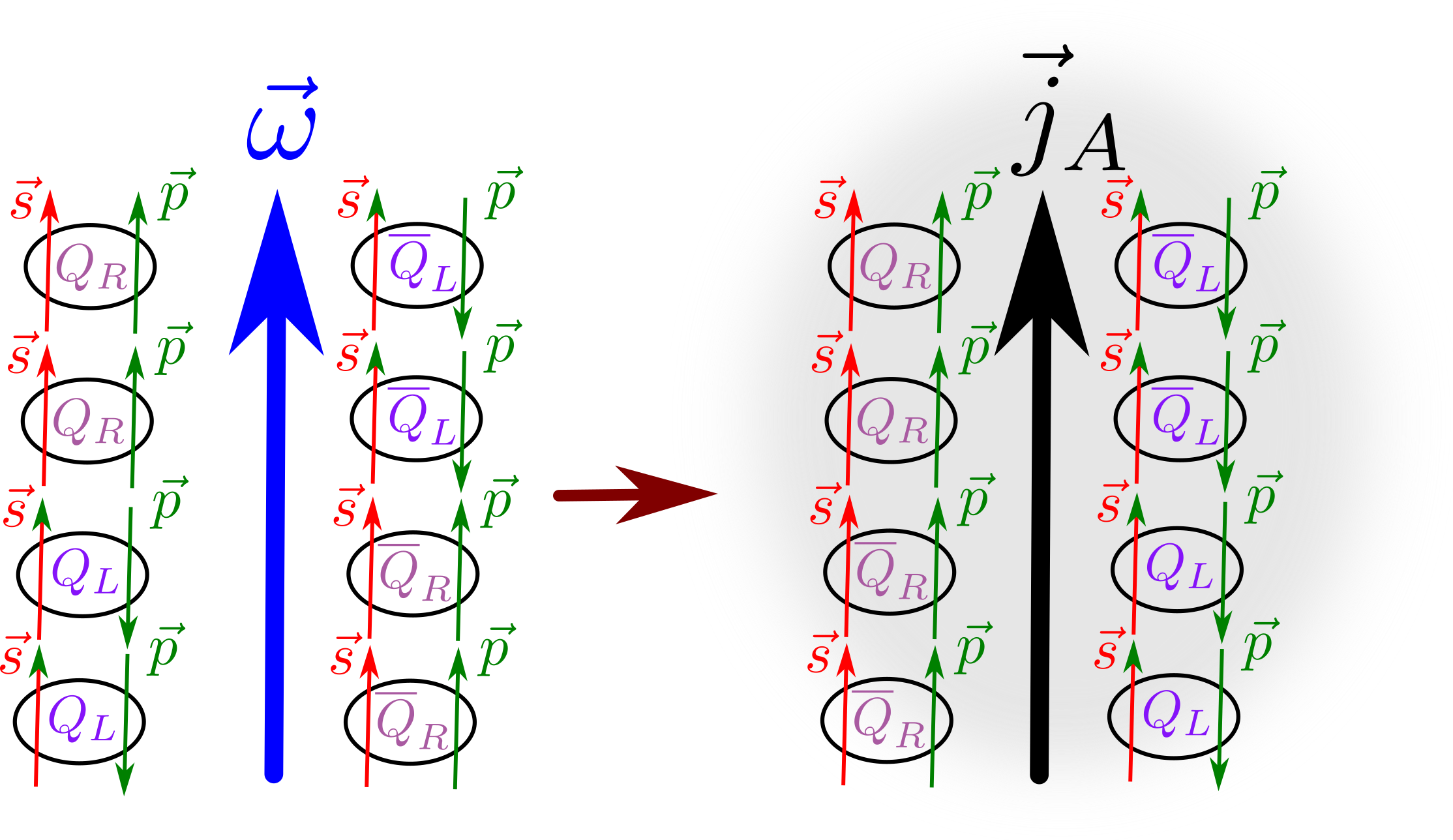
Figure 3.1: Illustration of the Axial Vortical Effect. To be specific, the illustration is for just one kind of massless quarks with electric charge $Q$ and for the case of $\mu_{\textup{A}}=\mu=0$. Even in the case of axial or electric imbalance, the axial current is aligned along the vorticity no matter what the signs of chemical potentials are.

The Axial Vortical Effect (AVE) states that in rotating fermion gas, an axial current is induced along rotation and consequently, the right and left chiral fermions get separated. This effect can be illustrated with a simple argument, which is strictly valid only for massless particles. In a rotating system, the fermion spin tends to align with the direction of rotation $\textstyle\mathbf{\omega}$ independently of their charge [107], in Fig. 3.1 for the sake of clarity all spin are aligned along rotation. The right-handed particles must have their momentum aligned with the spin, consequently will move in the direction of the spin, i.e. as shown in the right panel of Fig. 3.1 we get a net right-handed particles flow in the direction of $\textstyle\mathbf{\omega}$. On the other hand, the left-handed particles will move in the opposite direction, giving a net left-handed particles flow opposite to $\textstyle\mathbf{\omega}$. Together these flows give an axial current $\mathchoice{\mbox{\boldmath$\displaystyle\mathbf{j}$}}{\mbox{\boldmath$\textstyle\mathbf{j}$}}{\mbox{\boldmath$\scriptstyle\mathbf{j}$}}{\mbox{\boldmath$\scriptscriptstyle\mathbf{j}$}}_{\textup{A}}=n_{\textup{R}}\mathchoice{\mbox{\boldmath$\displaystyle\mathbf{v}$}}{\mbox{\boldmath$\textstyle\mathbf{v}$}}{\mbox{\boldmath$\scriptstyle\mathbf{v}$}}{\mbox{\boldmath$\scriptscriptstyle\mathbf{v}$}}_{\textup{R}}-n_{\textup{L}}\mathchoice{\mbox{\boldmath$\displaystyle\mathbf{v}$}}{\mbox{\boldmath$\textstyle\mathbf{v}$}}{\mbox{\boldmath$\scriptstyle\mathbf{v}$}}{\mbox{\boldmath$\scriptscriptstyle\mathbf{v}$}}_{\textup{L}}\propto\mathchoice{\mbox{\boldmath$\displaystyle\mathbf{\omega}$}}{\mbox{\boldmath$\textstyle\mathbf{\omega}$}}{\mbox{\boldmath$\scriptstyle\mathbf{\omega}$}}{\mbox{\boldmath$\scriptscriptstyle\mathbf{\omega}$}}$. A chiral or electric imbalance is not needed to reproduce the effect.

The very reason of the non-vanishing axial current is simply that it is allowed by the symmetry of the statistical operator, as recognized also in [76]. Indeed the current $\widehat{\mathchoice{\mbox{\boldmath$\displaystyle\mathbf{j}$}}{\mbox{\boldmath$\textstyle\mathbf{j}$}}{\mbox{\boldmath$\scriptstyle\mathbf{j}$}}{\mbox{\boldmath$\scriptscriptstyle\mathbf{j}$}}}_{\textup{A}}$ has the same properties of the angular momentum operator $\widehat{\mathchoice{\mbox{\boldmath$\displaystyle\mathbf{J}$}}{\mbox{\boldmath$\textstyle\mathbf{J}$}}{\mbox{\boldmath$\scriptstyle\mathbf{J}$}}{\mbox{\boldmath$\scriptscriptstyle\mathbf{J}$}}}$ under reflection, time reversal and charge conjugation; therefore its mean value is non vanishing

$$\mathchoice{\mbox{\boldmath$\displaystyle\mathbf{j}$}}{\mbox{\boldmath$\textstyle\mathbf{j}$}}{\mbox{\boldmath$\scriptstyle\mathbf{j}$}}{\mbox{\boldmath$\scriptscriptstyle\mathbf{j}$}}_{\textup{A}}=\frac{1}{\mathcal{Z}}{\text{tr}}\left[\mathchoice{\mbox{\boldmath$\displaystyle\mathbf{\widehat{j}}$}}{\mbox{\boldmath$\textstyle\mathbf{\widehat{j}}$}}{\mbox{\boldmath$\scriptstyle\mathbf{\widehat{j}}$}}{\mbox{\boldmath$\scriptscriptstyle\mathbf{\widehat{j}}$}}_{\textup{A}}\,\exp\left\{-\widehat{H}/T_{0}+\mathchoice{\mbox{\boldmath$\displaystyle\mathbf{\omega}$}}{\mbox{\boldmath$\textstyle\mathbf{\omega}$}}{\mbox{\boldmath$\scriptstyle\mathbf{\omega}$}}{\mbox{\boldmath$\scriptscriptstyle\mathbf{\omega}$}}\cdot\mathchoice{\mbox{\boldmath$\displaystyle\mathbf{\widehat{J}}$}}{\mbox{\boldmath$\textstyle\mathbf{\widehat{J}}$}}{\mbox{\boldmath$\scriptstyle\mathbf{\widehat{J}}$}}{\mbox{\boldmath$\scriptscriptstyle\mathbf{\widehat{J}}$}}/T_{0}\right\}\right]\neq 0.$$

Notice that this symmetry is classical; rotational symmetry is broken by fluid rotation not by quantum processes. For a free field, this procedure leads to the values of axial current reported in the previous section.

The AVE was originally addressed for neutrinos emitted by rotating black hole in ref. [98]. Lately, this effect was addressed in the context of Chiral Vortical Effect (CVE) and quantum anomalies [108, 76]. Several terms were found to contribute to the proportionality coefficient between $\mathchoice{\mbox{\boldmath$\displaystyle\mathbf{j}$}}{\mbox{\boldmath$\textstyle\mathbf{j}$}}{\mbox{\boldmath$\scriptstyle\mathbf{j}$}}{\mbox{\boldmath$\scriptscriptstyle\mathbf{j}$}}_{\textup{A}}$ and $\textstyle\mathbf{\omega}$, in the massless limit: a term proportional to the chiral potential $\mu_{\textup{A}}^{2}$ , also confirmed in holographic models [92, 90, 91, 93]; a term proportional to $T^{2}$ [77, 25, 56] whose existence was attributed to the gravitational anomaly  [109] and to the modular anomaly [74]. It is also worth pointing out that in fact, all calculations of the $T^{2}$ term in Eq. (3.56) in refs. [98, 25, 56] give the same result, i.e. $T^{2}/6$ like in Eq. (3.56). We would also like to point out that in the derivation of Vilenkin [98] it is clear that the effect is caused by the modified density operator in the presence of rotation, exactly like in our case, and indeed we recover the same result in Eq. (3.56).

We conclude this chapter motivating why the Axial Vortical Effect (AVE) is not to be ascribed to quantum anomalies, specifically chiral anomaly and gravitational anomaly. We understand that this statement goes against the conventional interpretation in literature, and yet some other authors have lately cast doubts about the anomalous origin of the AVE [110, 35].

Regarding chirality, we have called the AVE coefficient non-chiral because the corresponding correlator has even parity. As a consequence AVE does not vanish for $\zeta_{\textup{A}}=\mu_{\textup{A}}/T=0$, as it is apparent from Eq. (3.56). This means that the AVE does not need chiral imbalance to show up and persists for a perfectly chirally balanced system. This observation suggests that the AVE is not entirely dictated by the chiral anomaly. Furthermore, the connection with the chiral anomaly, namely the numerical factors in front of the chemical potentials in Eq. (3.56), is completely lost for a massive field. Indeed, AVE conductivity for massive filed was first found in [46, 35] and then in [60, 111, 65]. The chiral anomaly factor is recovered at high temperature, see Eq. (3.59), but it is lost at low temperature, see Eq. (3.60). Mass dependence also occurs similarly for the Chiral Separation Effect (CSE) coefficient [112], which is axial current induced by a magnetic field.

The temperature part of AVE is attributed to the gravitational anomaly or to be more specific to the mixed axial-gravitational anomaly, which is the term depending on curvature in chiral anomaly, see Eq. (1.7). Again, this connection, at least in the form presented in [109], is lost when we consider the AVE for a massive field, see for instance Eq. (3.60). Even in the case of a massless field, another evidence against the anomalous origin of AVE temperature term is that it receives radiative corrections by gauge interactions such as those of QED and QCD, as showed in [66, 24, 72, 113]. We also show in Sec. 4.4, that these radiative corrections are recovered and well explained in the global equilibrium model we are presenting. Thus, radiative corrections do not hinder the cause we are suggesting for AVE, i.e. the thermal states modified by rotation. On the contrary, quantum anomalies are exact results and should not receive correction above 1-loop diagrams. Gravitational anomaly is not exceptional to this feature. The fact that AVE does indeed receive such corrections is a clear sign that AVE could not be explained with (only) chiral and gravitational anomaly. Similar radiative corrections are found for CSE [114] but not for Chiral Magnetic Effect (CME) [115], whose relationship with the chiral anomaly is more consolidated.

Addressing the proper cause of the effect surely helps to understand the phenomena and therefore, to develop an accurate model to describe it. Knowing if it can be enhanced or diminished by mass or by the interactions is crucial when designing experiments aimed to present experimental evidence of such effects. The experimental manifestation of AVE, except the obvious axial-number separation, is linked to polarization. Indeed we showed that at global equilibrium, spin tensor alignment along rotation coincides with AVE, see Eq. (3.30). Since polarization is essentially the manifestation of spin-tensor anisotropy, corrections to AVE are directly transferred to polarization.

4  Chiral fermions under electromagnetic field

In this chapter, we consider the effects of an external electromagnetic field on the thermodynamics of chiral vorticous fluids. The effects of electromagnetic fields on relativistic quantum fluids is already a consolidated subject, see for instance [116] and reference therein and specifically for the effects of constant magnetic field on fermion gases see [117]. More recently, motivated by relativistic heavy-ion collisions, this topic has been addressed in [49] using the Zubarev’s non-equilibrium statistical operator that we are also using, and in [105] using generating functional and also with Wigner function using kinetic theory in [63, 64, 118].

In this chapter (and in a paper in preparation [119]), we want to study magnetized plasmas, highlighting the modifications caused by chirality and by thermal vorticity. First, we review the relativistic quantum theory of fermions under the effect of an external electromagnetic field. In the particular case of a constant homogeneous electromagnetic field, we discuss the symmetries of the theory and we provide the generators of those symmetries, which are the translations and a subgroup of Lorentz transformations. Then, we give exact solutions for thermal states of a system consisting of chiral fermions under an external constant magnetic field, which were not given before in literature using Zubarev’s density matrix formalism. We discuss the general properties of a system at thermal equilibrium with vorticity and electromagnetic field in Sec. 4.3. Since we derived exact solutions, we treat the electromagnetic field without approximation (at thermal equilibrium) and we consider the effect of thermal vorticity with linear response theory as done in the previous chapter. The consequences of electromagnetic field on chiral vortical effect and on axial vortical effect are analyzed. At last, we consider instead a dynamic gauge field and we compute the first-order radiative correction to the axial vortical effect conductivity.

4.1 Dirac Field in external electromagnetic field

Consider a Dirac field in external electromagnetic field. The Lagrangian of the theory is given by Eq. (1.2), which in flat space-time reads:

$$\mathcal{L}=\frac{{\rm i}}{2}\left[\bar{\psi}\gamma^{\mu}\overrightarrow{\partial}_{\mu}\psi-\bar{\psi}\gamma^{\mu}\overleftarrow{\partial}_{\mu}\psi\right]-m\bar{\psi}\psi-j^{\mu}A_{\mu},$$

with $\widehat{j}^{\mu}=q\bar{\psi}\gamma^{\mu}\psi$ and where $q$ is the elementary electric charge of the field and where the gauge potential $A^{\mu}$ is an external non dynamic field. This Lagrangian is the same as the one obtained from the free Dirac Lagrangian via the minimal coupling substitution $\partial_{\mu}\to\partial_{\mu}+{\rm i}qA_{\mu}$, which grants gauge invariance to the theory. From Euler Eq.s we obtain the equations of motion (EOM) for the Dirac field:

$$\not{\partial}\psi=-{\rm i}(q\not{A}+m)\psi,\quad\not{\partial}\bar{\psi}=\bar{\psi}{\rm i}(q\not{A}+m).$$

From the EOM it is straightforward to verify that the electric current is conserved $\partial_{\mu}\widehat{j}^{\mu}=0$. We can also use the minimal substitution

$$\overrightarrow{\partial}\to\overrightarrow{\nabla}_{\mu}=\overrightarrow{\partial}_{\mu}+{\rm i}qA_{\mu},\quad\overleftarrow{\partial}\to\overleftarrow{\nabla}_{\mu}=\overleftarrow{\partial}_{\mu}-{\rm i}qA_{\mu}$$

in the canonical stress-energy tensor of the free theory to obtain the stress-energy tensor of fermions in external electromagnetic field:

$$\widehat{T}^{\mu\nu}=\frac{{\rm i}}{2}\left[\bar{\psi}\gamma^{\mu}\overrightarrow{\partial}^{\nu}\psi-\bar{\psi}\gamma^{\mu}\overleftarrow{\partial}^{\nu}\psi\right]-\widehat{j}^{\mu}A^{\nu}.$$

Again, with the EOM (see Appendix B for second order equations) we can verify that the stress-energy tensor is not conserved but it is driven by Lorentz force:

$$\partial^{\mu}\widehat{T}_{\mu\nu}=\widehat{j}^{\lambda}F_{\nu\lambda}.$$ (4.1)

We can show (see Appendix B) that the correct symmetrization of this stress-energy tensor that leaves the previous operator relations unmodified is

$$\widehat{T}^{\mu\nu}=\frac{{\rm i}}{4}\left[\bar{\psi}\gamma^{\mu}\overrightarrow{\partial}^{\nu}\psi-\bar{\psi}\gamma^{\mu}\overleftarrow{\partial}^{\nu}\psi+\bar{\psi}\gamma^{\nu}\overrightarrow{\partial}^{\mu}\psi-\bar{\psi}\gamma^{\nu}\overleftarrow{\partial}^{\mu}\psi\right]-\frac{1}{2}\left(\widehat{j}^{\mu}A^{\nu}+\widehat{j}^{\nu}A^{\mu}\right);$$

note that this is the stress-energy tensor we would obtain using the minimal substitution to the symmetric stress-energy tensor of free Dirac field.

4.1.1 Symmetries in constant homogeneous electromagnetic field

It is worth noticing that the symmetries of the theory of fermions in external electromagnetic field are different from those of free fermions or those of quantum electrodynamics. Indeed while a system without external forces is symmetric for the full Poincaré group, some of the symmetries are lost when external fields are considered, because those do not transform together with the rest of the system. Here we discuss the symmetries of the system in the particular case of a constant homogeneous electromagnetic field. We examine the transformations that are still symmetries of the theory, the consequent conserved quantities of the system and the form of the generators of such transformations.

If the Lagrangian of our theory is invariant under translations, by Noether’s theorem we can identify and we can construct four operators that share three properties: they are conserved quantities, they are the generators of translations and they constitute the four-momentum of the system. However, translational invariance by itself does not guarantees that only a single quantity must have all the three above properties altogether. Consider again a system under an external electromagnetic field. In this situation, Poincaré symmetry of space-time is broken. Let the electromagnetic field be constant and homogeneous, then translational invariance is still present. However, the Lagrangian is not invariant under space-time translation, but it acquires a term that is a four-divergence. This term, under appropriate boundary conditions, does not affect the action of the system and the overall invariance is preserved. Nevertheless, the consequence of the additional term is that we can distinguish three different operators, each of them having one of the three properties stated above. This is understood with the Noether-Tassie-Buchdahl theorem [120, 121, 122]: given a Lagrangian $\mathcal{L}(\psi(x),\partial_{\mu}\psi(x),x)$ and the infinitesimal transformation $x^{\prime\mu}=x^{\mu}+\delta x^{\mu}$, $\psi^{\prime}=\psi+\delta\psi$ such that $\partial_{\mu}\delta x^{\mu}=0$, which transforms the Lagrangian in

$$\mathcal{L}(\psi^{\prime}(x^{\prime}),\partial^{\prime}_{\mu}\psi^{\prime}(x^{\prime}),x^{\prime})=\mathcal{L}(\psi(x),\partial_{\mu}\psi(x),x)+\partial_{\mu}X^{\mu},$$

where $X^{\mu}$ is a functional depending exclusively on $\psi(x)$ and $x$, then the quantity

$$\Gamma^{\mu}=\frac{\delta\mathcal{L}}{\delta\partial_{\mu}\psi}\delta\psi-\left(\frac{\delta\mathcal{L}}{\delta\partial_{\mu}\psi}\partial_{\nu}\psi-\mathcal{L}\,g^{\mu}_{\,\nu}\right)\delta x^{\nu}-X^{\mu}$$

is conserved, i.e. divergence-less.

Consider the Dirac Lagrangian in constant homogeneous electromagnetic field

$$\mathcal{L}(\psi(x),\partial_{\mu}\psi(x),x)=\bar{\psi}({\rm i}\not{\partial}-m)\psi-\widehat{j}^{\mu}A_{\mu}.$$

The translation transformation ($\delta\psi=0$, $\delta x^{\mu}=\epsilon^{\mu}$) acts on the Dirac field but does not act directly to the external gauge field. Therefore, the Lagrangian variation by translation is

$$\begin{split}\delta\mathcal{L}=&\mathcal{L}(\psi^{\prime}(x^{\prime}),\partial^{\prime}_{\mu}\psi^{\prime}(x^{\prime}),x^{\prime})-\mathcal{L}(\psi(x),\partial_{\mu}\psi(x),x)\\ =&\widehat{j}^{\mu}\partial_{\nu}A_{\mu}\epsilon^{\nu}=\widehat{j}^{\mu}(F_{\nu\mu}+\partial_{\mu}A_{\nu})\epsilon^{\nu}=-\widehat{j}^{\mu}(F_{\mu\nu}-\partial_{\mu}A_{\nu})\epsilon^{\nu}.\end{split}$$

We can then identify the quantity $X$ of Noether-Tassie-Buchdahl theorem

$$X^{\mu\nu}\equiv\widehat{j}^{\mu}(A^{\nu}+F^{\nu\lambda}x_{\lambda}).$$

Indeed its divergence is the variation of the Lagrangian

$$\epsilon_{\nu}\partial_{\mu}X^{\mu\nu}=(\partial_{\mu}\widehat{j}^{\mu})(A^{\nu}+F^{\nu\lambda}x_{\lambda})\epsilon_{\nu}+\widehat{j}^{\mu}(\partial_{\mu}A_{\nu}+F_{\nu\mu})\epsilon^{\nu}=-\widehat{j}^{\mu}(F_{\mu\nu}-\partial_{\mu}A_{\nu})\epsilon^{\nu}=\delta\mathcal{L},$$

therefore, the theorem implies that the system has a canonical conserved tensor given by:

$$\widehat{\pi}^{\mu\nu}_{\textup{can}}=\widehat{T}^{\mu\nu}_{0}-\widehat{j}^{\mu}A^{\nu}-\widehat{j}^{\mu}F^{\nu\lambda}x_{\lambda},$$

where $\widehat{T}^{\mu\nu}_{0}$ is the free canonical Dirac stress-energy tensor. Using Belinfante procedure (see Appendix B) we can transform $\widehat{T}^{\mu\nu}_{0}-\widehat{j}^{\mu}A^{\nu}$ into the symmetric stress-energy tensor of Dirac field in external magnetic field $\widehat{T}^{\mu\nu}_{S}$ and the above conserved tensor becomes:

$$\widehat{\pi}^{\mu\nu}\equiv\widehat{T}^{\mu\nu}_{S}-\widehat{j}^{\mu}F^{\nu\lambda}x_{\lambda}.$$ (4.2)

From the above equation, we can simply verify that $\partial_{\mu}\widehat{\pi}^{\mu\nu}=0$ form Eq. (4.1). However, note that $\widehat{\pi}^{\mu\nu}$ is not symmetric and that it is gauge invariant. The conserved quantities related to this quantities are the four vectors

$$\widehat{\pi}^{\mu}=\int\mathrm{d}^{3}x\,\widehat{\pi}^{0\mu}$$

and they also constitute the generator of the translations [122]. The momentum of the system is still given by

$$\widehat{P}^{\mu}=\int\mathrm{d}^{3}x\,\widehat{T}^{0\mu}$$

but it is not a conserved quantity and it is not the generator of translations. Another difference from four-momenta is that different components of this vectors do not commute, instead they satisfy [122]:

$$[\widehat{\pi}^{\mu},\widehat{\pi}^{\nu}]={\rm i}\widehat{Q}F^{\mu\nu},$$

where $\widehat{Q}$ is the electric charge operator.

As for Lorentz’s transformations, we expect that the variation of the Lagrangian is a full divergence only for specific forms of transformations. For example, with a vanishing electric field and a constant magnetic field, only the rotation along the direction of the magnetic field and the boost along the magnetic field are symmetries of the theory. Therefore, only in these cases, the Lagrangian variation could be vanishing or a full divergence.

Returning to the general case, we can repeat the previous argument of translations to the Lorentz transformation: $\delta x^{\mu}=\omega^{\mu\nu}x_{\nu},\,\delta\psi=-\frac{{\rm i}}{2}\omega_{\mu\nu}\sigma^{\mu\nu}\psi$; we find that the transformed Lagrangian is

$$\begin{split}\delta\mathcal{L}=&\omega^{\mu\nu}\widehat{j}^{\lambda}(g_{\mu\lambda}A_{\nu}-g_{\nu\lambda}A_{\mu}+x_{\mu}\partial_{\nu}A_{\lambda}-x_{\nu}\partial_{\mu}A_{\lambda})\\ =&\omega^{\mu\nu}\widehat{j}^{\lambda}\left[\partial_{\lambda}\left(x_{\mu}A_{\nu}-x_{\nu}A_{\mu}\right)-x_{\mu}\partial_{\lambda}A_{\nu}+x_{\mu}\partial_{\nu}A_{\lambda}+x_{\nu}\partial_{\lambda}A_{\mu}-x_{\nu}\partial_{\mu}A_{\lambda}\right]\\ =&\omega^{\mu\nu}\widehat{j}^{\lambda}\left[\partial_{\lambda}\left(x_{\mu}A_{\nu}-x_{\nu}A_{\mu}\right)+x_{\mu}F_{\nu\lambda}-x_{\nu}F_{\mu\lambda}\right].\end{split}$$

It is straightforward to check the identities:

$$\omega^{\mu\nu}x_{\mu}F_{\nu\lambda}=x^{\rho}\omega_{\rho\sigma}F^{\sigma}_{\,\,\lambda},$$

$$\omega^{\mu\nu}x_{\mu}F_{\nu\lambda}=-\omega^{\mu\nu}\partial_{\lambda}(x_{\mu}x^{\sigma}F_{\sigma\nu})-x^{\rho}\omega_{\lambda\sigma}F^{\sigma}_{\,\,\rho},$$

from which it follows

$$\begin{split}\omega^{\mu\nu}x_{\mu}F_{\nu\lambda}=&\frac{1}{2}\omega^{\mu\nu}x_{\mu}F_{\nu\lambda}+\frac{1}{2}\omega^{\mu\nu}x_{\mu}F_{\nu\lambda}\\ =&-\frac{1}{2}\omega^{\mu\nu}\partial_{\lambda}(x_{\mu}x^{\sigma}F_{\sigma\nu})-\frac{1}{2}x^{\rho}(\omega_{\lambda\sigma}F^{\sigma}_{\,\,\rho}-\omega_{\rho\sigma}F^{\sigma}_{\,\,\lambda}),\end{split}$$

and similarly

$$\omega^{\mu\nu}x_{\nu}F_{\mu\lambda}=\frac{1}{2}\omega^{\mu\nu}\partial_{\lambda}(x_{\nu}x^{\sigma}F_{\sigma\mu})-\frac{1}{2}x^{\rho}(\omega_{\lambda\sigma}F^{\sigma}_{\,\,\rho}-\omega_{\rho\sigma}F^{\sigma}_{\,\,\lambda}).$$

Therefore, the Lagrangian variation becomes

$$\begin{split}\delta\mathcal{L}=&\frac{1}{2}\omega^{\mu\nu}\partial_{\lambda}\left[\widehat{j}^{\lambda}x_{\mu}\left(A_{\nu}-\frac{1}{2}x^{\sigma}F_{\sigma\nu}\right)-\widehat{j}^{\lambda}x_{\nu}\left(A_{\mu}-\frac{1}{2}x^{\sigma}F_{\sigma\mu}\right)\right]\\ &-\frac{1}{2}x^{\rho}\widehat{j}^{\lambda}(\omega_{\lambda\sigma}F^{\sigma}_{\,\,\rho}-\omega_{\rho\sigma}F^{\sigma}_{\,\,\lambda}).\end{split}$$

The first part of r.h.s. is written as a four-divergence. The remaining part can not be cast into a four-divergence but it is proportional to the following product

$$(\omega\wedge F)_{\lambda\rho}=\omega_{\lambda\sigma}F^{\sigma}_{\,\,\rho}-\omega_{\rho\sigma}F^{\sigma}_{\,\,\lambda}.$$

The product of two non-vanishing anti-symmetric tensor of rank two, $\omega\wedge F$, is zero if and only if $\omega$ is a linear combination of $F$ and its dual $F^{*}$ (or viceversa):

$$(\omega\wedge F)_{\lambda\rho}=0\quad\text{iff}\quad\omega_{\mu\nu}=k\,F_{\mu\nu}+k^{\prime}\,F^{*}_{\mu\nu},\quad k,k^{\prime}\in\mathbb{R}.$$ (4.3)

The previous statement can be proven by denoting the tensor with the “electric” and “magnetic” vectors

$$F=(\mathchoice{\mbox{\boldmath$\displaystyle\mathbf{E}$}}{\mbox{\boldmath$\textstyle\mathbf{E}$}}{\mbox{\boldmath$\scriptstyle\mathbf{E}$}}{\mbox{\boldmath$\scriptscriptstyle\mathbf{E}$}},\mathchoice{\mbox{\boldmath$\displaystyle\mathbf{B}$}}{\mbox{\boldmath$\textstyle\mathbf{B}$}}{\mbox{\boldmath$\scriptstyle\mathbf{B}$}}{\mbox{\boldmath$\scriptscriptstyle\mathbf{B}$}}),\quad\quad\text{meaning}\quad E^{i}=F^{0i},\quad B^{i}=\frac{1}{2}\epsilon^{ijk}F_{jk},$$

$$\omega=(\mathchoice{\mbox{\boldmath$\displaystyle\mathbf{\alpha}$}}{\mbox{\boldmath$\textstyle\mathbf{\alpha}$}}{\mbox{\boldmath$\scriptstyle\mathbf{\alpha}$}}{\mbox{\boldmath$\scriptscriptstyle\mathbf{\alpha}$}},\mathchoice{\mbox{\boldmath$\displaystyle\mathbf{w}$}}{\mbox{\boldmath$\textstyle\mathbf{w}$}}{\mbox{\boldmath$\scriptstyle\mathbf{w}$}}{\mbox{\boldmath$\scriptscriptstyle\mathbf{w}$}}),\quad\quad\text{meaning}\quad\alpha^{i}=\omega^{0i},\quad w^{i}=\frac{1}{2}\epsilon^{ijk}\omega_{jk}.$$

Then, with this notation, the wedge product can be written as

$$\omega\wedge F=(\mathchoice{\mbox{\boldmath$\displaystyle\mathbf{\alpha}$}}{\mbox{\boldmath$\textstyle\mathbf{\alpha}$}}{\mbox{\boldmath$\scriptstyle\mathbf{\alpha}$}}{\mbox{\boldmath$\scriptscriptstyle\mathbf{\alpha}$}}\times\mathchoice{\mbox{\boldmath$\displaystyle\mathbf{B}$}}{\mbox{\boldmath$\textstyle\mathbf{B}$}}{\mbox{\boldmath$\scriptstyle\mathbf{B}$}}{\mbox{\boldmath$\scriptscriptstyle\mathbf{B}$}}+\mathchoice{\mbox{\boldmath$\displaystyle\mathbf{w}$}}{\mbox{\boldmath$\textstyle\mathbf{w}$}}{\mbox{\boldmath$\scriptstyle\mathbf{w}$}}{\mbox{\boldmath$\scriptscriptstyle\mathbf{w}$}}\times\mathchoice{\mbox{\boldmath$\displaystyle\mathbf{E}$}}{\mbox{\boldmath$\textstyle\mathbf{E}$}}{\mbox{\boldmath$\scriptstyle\mathbf{E}$}}{\mbox{\boldmath$\scriptscriptstyle\mathbf{E}$}},\,\mathchoice{\mbox{\boldmath$\displaystyle\mathbf{w}$}}{\mbox{\boldmath$\textstyle\mathbf{w}$}}{\mbox{\boldmath$\scriptstyle\mathbf{w}$}}{\mbox{\boldmath$\scriptscriptstyle\mathbf{w}$}}\times\mathchoice{\mbox{\boldmath$\displaystyle\mathbf{B}$}}{\mbox{\boldmath$\textstyle\mathbf{B}$}}{\mbox{\boldmath$\scriptstyle\mathbf{B}$}}{\mbox{\boldmath$\scriptscriptstyle\mathbf{B}$}}-\mathchoice{\mbox{\boldmath$\displaystyle\mathbf{\alpha}$}}{\mbox{\boldmath$\textstyle\mathbf{\alpha}$}}{\mbox{\boldmath$\scriptstyle\mathbf{\alpha}$}}{\mbox{\boldmath$\scriptscriptstyle\mathbf{\alpha}$}}\times\mathchoice{\mbox{\boldmath$\displaystyle\mathbf{E}$}}{\mbox{\boldmath$\textstyle\mathbf{E}$}}{\mbox{\boldmath$\scriptstyle\mathbf{E}$}}{\mbox{\boldmath$\scriptscriptstyle\mathbf{E}$}}).$$

Then at each tensor one can associate a complex three-vector

$$F\to\mathchoice{\mbox{\boldmath$\displaystyle\mathbf{F}$}}{\mbox{\boldmath$\textstyle\mathbf{F}$}}{\mbox{\boldmath$\scriptstyle\mathbf{F}$}}{\mbox{\boldmath$\scriptscriptstyle\mathbf{F}$}}=\mathchoice{\mbox{\boldmath$\displaystyle\mathbf{B}$}}{\mbox{\boldmath$\textstyle\mathbf{B}$}}{\mbox{\boldmath$\scriptstyle\mathbf{B}$}}{\mbox{\boldmath$\scriptscriptstyle\mathbf{B}$}}+{\rm i}\mathchoice{\mbox{\boldmath$\displaystyle\mathbf{E}$}}{\mbox{\boldmath$\textstyle\mathbf{E}$}}{\mbox{\boldmath$\scriptstyle\mathbf{E}$}}{\mbox{\boldmath$\scriptscriptstyle\mathbf{E}$}},\quad\quad\omega\to\mathchoice{\mbox{\boldmath$\displaystyle\mathbf{\omega}$}}{\mbox{\boldmath$\textstyle\mathbf{\omega}$}}{\mbox{\boldmath$\scriptstyle\mathbf{\omega}$}}{\mbox{\boldmath$\scriptscriptstyle\mathbf{\omega}$}}=\mathchoice{\mbox{\boldmath$\displaystyle\mathbf{w}$}}{\mbox{\boldmath$\textstyle\mathbf{w}$}}{\mbox{\boldmath$\scriptstyle\mathbf{w}$}}{\mbox{\boldmath$\scriptscriptstyle\mathbf{w}$}}+{\rm i}\mathchoice{\mbox{\boldmath$\displaystyle\mathbf{\alpha}$}}{\mbox{\boldmath$\textstyle\mathbf{\alpha}$}}{\mbox{\boldmath$\scriptstyle\mathbf{\alpha}$}}{\mbox{\boldmath$\scriptscriptstyle\mathbf{\alpha}$}}$$

and the wedge product becomes

$$\omega\wedge F\to\mathchoice{\mbox{\boldmath$\displaystyle\mathbf{\omega}$}}{\mbox{\boldmath$\textstyle\mathbf{\omega}$}}{\mbox{\boldmath$\scriptstyle\mathbf{\omega}$}}{\mbox{\boldmath$\scriptscriptstyle\mathbf{\omega}$}}\times\mathchoice{\mbox{\boldmath$\displaystyle\mathbf{F}$}}{\mbox{\boldmath$\textstyle\mathbf{F}$}}{\mbox{\boldmath$\scriptstyle\mathbf{F}$}}{\mbox{\boldmath$\scriptscriptstyle\mathbf{F}$}}=(\mathchoice{\mbox{\boldmath$\displaystyle\mathbf{w}$}}{\mbox{\boldmath$\textstyle\mathbf{w}$}}{\mbox{\boldmath$\scriptstyle\mathbf{w}$}}{\mbox{\boldmath$\scriptscriptstyle\mathbf{w}$}}+{\rm i}\mathchoice{\mbox{\boldmath$\displaystyle\mathbf{\alpha}$}}{\mbox{\boldmath$\textstyle\mathbf{\alpha}$}}{\mbox{\boldmath$\scriptstyle\mathbf{\alpha}$}}{\mbox{\boldmath$\scriptscriptstyle\mathbf{\alpha}$}})\times(\mathchoice{\mbox{\boldmath$\displaystyle\mathbf{B}$}}{\mbox{\boldmath$\textstyle\mathbf{B}$}}{\mbox{\boldmath$\scriptstyle\mathbf{B}$}}{\mbox{\boldmath$\scriptscriptstyle\mathbf{B}$}}+{\rm i}\mathchoice{\mbox{\boldmath$\displaystyle\mathbf{E}$}}{\mbox{\boldmath$\textstyle\mathbf{E}$}}{\mbox{\boldmath$\scriptstyle\mathbf{E}$}}{\mbox{\boldmath$\scriptscriptstyle\mathbf{E}$}}).$$

It is now clear that the product is vanishing when $\textstyle\mathbf{\omega}$ is parallel to $\textstyle\mathbf{F}$, this occur if they are proportional:

$$(\mathchoice{\mbox{\boldmath$\displaystyle\mathbf{w}$}}{\mbox{\boldmath$\textstyle\mathbf{w}$}}{\mbox{\boldmath$\scriptstyle\mathbf{w}$}}{\mbox{\boldmath$\scriptscriptstyle\mathbf{w}$}}+{\rm i}\mathchoice{\mbox{\boldmath$\displaystyle\mathbf{\alpha}$}}{\mbox{\boldmath$\textstyle\mathbf{\alpha}$}}{\mbox{\boldmath$\scriptstyle\mathbf{\alpha}$}}{\mbox{\boldmath$\scriptscriptstyle\mathbf{\alpha}$}})=(a+{\rm i}\,b)(\mathchoice{\mbox{\boldmath$\displaystyle\mathbf{B}$}}{\mbox{\boldmath$\textstyle\mathbf{B}$}}{\mbox{\boldmath$\scriptstyle\mathbf{B}$}}{\mbox{\boldmath$\scriptscriptstyle\mathbf{B}$}}+{\rm i}\mathchoice{\mbox{\boldmath$\displaystyle\mathbf{E}$}}{\mbox{\boldmath$\textstyle\mathbf{E}$}}{\mbox{\boldmath$\scriptstyle\mathbf{E}$}}{\mbox{\boldmath$\scriptscriptstyle\mathbf{E}$}}),\quad a,b\in\mathbb{R}.$$

This is equivalent to say that $\textstyle\mathbf{\omega}$ is a real combination of $\mathchoice{\mbox{\boldmath$\displaystyle\mathbf{B}$}}{\mbox{\boldmath$\textstyle\mathbf{B}$}}{\mbox{\boldmath$\scriptstyle\mathbf{B}$}}{\mbox{\boldmath$\scriptscriptstyle\mathbf{B}$}}+{\rm i}\mathchoice{\mbox{\boldmath$\displaystyle\mathbf{E}$}}{\mbox{\boldmath$\textstyle\mathbf{E}$}}{\mbox{\boldmath$\scriptstyle\mathbf{E}$}}{\mbox{\boldmath$\scriptscriptstyle\mathbf{E}$}}$ and $\mathchoice{\mbox{\boldmath$\displaystyle\mathbf{B}$}}{\mbox{\boldmath$\textstyle\mathbf{B}$}}{\mbox{\boldmath$\scriptstyle\mathbf{B}$}}{\mbox{\boldmath$\scriptscriptstyle\mathbf{B}$}}-{\rm i}\mathchoice{\mbox{\boldmath$\displaystyle\mathbf{E}$}}{\mbox{\boldmath$\textstyle\mathbf{E}$}}{\mbox{\boldmath$\scriptstyle\mathbf{E}$}}{\mbox{\boldmath$\scriptscriptstyle\mathbf{E}$}}$, or that we have two independent solutions of Eq. (4.19): $\omega=k(\mathchoice{\mbox{\boldmath$\displaystyle\mathbf{E}$}}{\mbox{\boldmath$\textstyle\mathbf{E}$}}{\mbox{\boldmath$\scriptstyle\mathbf{E}$}}{\mbox{\boldmath$\scriptscriptstyle\mathbf{E}$}},\mathchoice{\mbox{\boldmath$\displaystyle\mathbf{B}$}}{\mbox{\boldmath$\textstyle\mathbf{B}$}}{\mbox{\boldmath$\scriptstyle\mathbf{B}$}}{\mbox{\boldmath$\scriptscriptstyle\mathbf{B}$}})=kF$ and $\omega=k^{\prime}(-\mathchoice{\mbox{\boldmath$\displaystyle\mathbf{B}$}}{\mbox{\boldmath$\textstyle\mathbf{B}$}}{\mbox{\boldmath$\scriptstyle\mathbf{B}$}}{\mbox{\boldmath$\scriptscriptstyle\mathbf{B}$}},\mathchoice{\mbox{\boldmath$\displaystyle\mathbf{E}$}}{\mbox{\boldmath$\textstyle\mathbf{E}$}}{\mbox{\boldmath$\scriptstyle\mathbf{E}$}}{\mbox{\boldmath$\scriptscriptstyle\mathbf{E}$}})=k^{\prime}F^{*}$, with $k$ and $k^{\prime}$ real numbers. Therefore, we proved that the part of Lagrangian variation which is not a divergence is vanishing when $\omega^{\mu\nu}$ is a linear combination of electromagnetic stress-energy tensor and its dual:

$$\omega^{\mu\nu}=a\,F^{\mu\nu}+\frac{b}{2}\epsilon^{\mu\nu\rho\sigma}F_{\rho\sigma}.$$ (4.4)

This means, as expected, that the action and the theory is invariant only under certain type of Lorentz transformations: the ones generated with a parameter of the form (4.4). For example, in the case of constant magnetic field, we recover that the system is invariant only for rotation and boost along the magnetic field. Set then $\omega$ either as $\omega_{\mu\nu}\propto F_{\mu\nu}$ or $\omega_{\mu\nu}\propto F^{*}_{\mu\nu}$, so that the Lagrangian variation is a four-divergence, from Noether-Tassie-Buchdahl theorem, the two following quantities are divergence-less:

$$\widehat{\Gamma}^{\lambda}=\frac{1}{2}F^{\mu\nu}\left[x_{\mu}\left(\widehat{T}^{\lambda}_{0\,\,\nu}-\widehat{j}^{\lambda}A_{\nu}+\frac{1}{2}\widehat{j}^{\lambda}x^{\rho}F_{\rho\nu}\right)-x_{\nu}\left(\widehat{T}^{\lambda}_{0\,\,\mu}-\widehat{j}^{\lambda}A_{\mu}+\frac{1}{2}\widehat{j}^{\lambda}x^{\rho}F_{\rho\mu}\right)+\widehat{S}^{\lambda}_{\,\mu\nu}\right],$$

$$\widehat{\Gamma}^{*\lambda}=\frac{1}{2}F^{*\mu\nu}\left[x_{\mu}\left(\widehat{T}^{\lambda}_{0\,\,\nu}-\widehat{j}^{\lambda}A_{\nu}+\frac{1}{2}\widehat{j}^{\lambda}x^{\rho}F_{\rho\nu}\right)-x_{\nu}\left(\widehat{T}^{\lambda}_{0\,\,\mu}-\widehat{j}^{\lambda}A_{\mu}+\frac{1}{2}\widehat{j}^{\lambda}x^{\rho}F_{\rho\mu}\right)+\widehat{S}^{\lambda}_{\,\mu\nu}\right],$$

with $\widehat{S}^{\lambda}_{\mu\nu}$ the canonical spin tensor of free Dirac field. After Belinfante transformation, the quantities become

$$\begin{split}\widehat{\Gamma}^{\lambda}=&\frac{1}{2}F^{\mu\nu}\widehat{M}^{\lambda}_{\mu\nu},\quad\widehat{\Gamma}^{*\lambda}=\frac{1}{2}F^{*\mu\nu}\widehat{M}^{\lambda}_{\mu\nu},\\ \widehat{M}^{\lambda}_{\mu\nu}\equiv&x_{\mu}\left(\widehat{T}^{\lambda}_{S\,\nu}+\frac{1}{2}\widehat{j}^{\lambda}x^{\rho}F_{\rho\nu}\right)-x_{\nu}\left(\widehat{T}^{\lambda}_{S\,\mu}+\frac{1}{2}\widehat{j}^{\lambda}x^{\rho}F_{\rho\mu}\right)\\ =&x_{\mu}\left(\widehat{\pi}^{\lambda}_{\,\,\nu}-\frac{1}{2}\widehat{j}^{\lambda}x^{\rho}F_{\rho\nu}\right)-x_{\nu}\left(\widehat{\pi}^{\lambda}_{\,\,\mu}-\frac{1}{2}\widehat{j}^{\lambda}x^{\rho}F_{\rho\mu}\right).\end{split}$$ (4.5)

We can define the integrals:

$$\widehat{M}_{\mu\nu}=\int\mathrm{d}^{3}x\,\widehat{M}^{0}_{\mu\nu},$$

which are conserved quantities only if projected with $F^{\mu\nu}$ and $F^{*\mu\nu}$. The operators $\widehat{M}_{\mu\nu}$ are the generators of Lorentz transformations if they are also a symmetry for the theory, otherwise the Wigner’s theorem does not applies and we can not say that such transformations admit an unitary and linear (or anti-unitary and anti-linear) representation. For those operators, the following Algebra holds [122]:

$$\begin{split}[\widehat{\pi}^{\mu},\widehat{\pi}^{\nu}]=&{\rm i}F^{\mu\nu}\widehat{Q},\\ \frac{1}{2}F_{\rho\sigma}[\widehat{\pi}^{\mu},\widehat{M}^{\rho\sigma}]=&\frac{{\rm i}}{2}F_{\rho\sigma}\left(\eta^{\mu\rho}\widehat{\pi}^{\sigma}-\eta^{\mu\sigma}\widehat{\pi}^{\rho}\right),\\ \frac{1}{2}F^{*}_{\rho\sigma}[\widehat{\pi}^{\mu},\widehat{M}^{\rho\sigma}]=&\frac{{\rm i}}{2}F^{*}_{\rho\sigma}\left(\eta^{\mu\rho}\widehat{\pi}^{\sigma}-\eta^{\mu\sigma}\widehat{\pi}^{\rho}\right),\end{split}$$ (4.6)

where $\widehat{Q}$ is the electric charge operator. In the particular case of vanishing electric field and constant magnetic field along the $z$ axis, the Algebra becomes:

$$[\widehat{\pi}_{x},\,\widehat{\pi}_{y}]={\rm i}|\mathchoice{\mbox{\boldmath$\displaystyle\mathbf{B}$}}{\mbox{\boldmath$\textstyle\mathbf{B}$}}{\mbox{\boldmath$\scriptstyle\mathbf{B}$}}{\mbox{\boldmath$\scriptscriptstyle\mathbf{B}$}}|\widehat{Q},$$

$$[\widehat{J}_{z},\widehat{\pi}_{x}]={\rm i}\widehat{\pi}_{y},\quad[\widehat{J}_{z},\widehat{\pi}_{y}]=-{\rm i}\widehat{\pi}_{x},$$

$$[\widehat{K}_{z},\widehat{\pi}_{t}]=-{\rm i}\widehat{\pi}_{z},\quad[\widehat{K}_{z},\widehat{\pi}_{z}]=-{\rm i}\widehat{\pi}_{t}.$$

4.2 Chiral fermions in constant magnetic field

Consider now a system consisting of chiral fermions in an external homogeneous constant magnetic field $\textstyle\mathbf{B}$ at thermal equilibrium with vanishing thermal vorticity. The system Lagrangian and EOM were discussed in the previous section. The local thermal equilibrium density operator is given by Eq. (1.11) with the addition of an axial current:

$$\widehat{\rho}_{\textup{LTE}}=\frac{1}{Z}\exp\left[-\int_{\Sigma}\mathrm{d}\Sigma_{\mu}\left(\widehat{T}^{\mu\nu}(x)\beta_{\nu}(x)-\zeta(x)\,\widehat{j}^{\mu}(x)-\zeta_{\textup{A}}(x)\,\widehat{j}_{\textup{A}}^{\mu}(x)\right)\right],$$

where the operators are defined (see previous Section) as

$$\begin{split}\widehat{j}^{\,\mu}=&\,q\bar{\psi}\gamma^{\mu}\psi,\quad\widehat{j}^{\,\mu}_{\textup{A}}=\,\bar{\psi}\gamma^{\mu}\gamma^{5}\psi,\\ \widehat{T}^{\mu\nu}=&\frac{{\rm i}}{4}\left[\bar{\psi}\gamma^{\mu}\overrightarrow{\partial}^{\nu}\psi-\bar{\psi}\gamma^{\mu}\overleftarrow{\partial}^{\nu}\psi+\bar{\psi}\gamma^{\nu}\overrightarrow{\partial}^{\mu}\psi-\bar{\psi}\gamma^{\nu}\overleftarrow{\partial}^{\mu}\psi\right]-\frac{1}{2}\left(\widehat{j}^{\mu}A^{\nu}+\widehat{j}^{\nu}A^{\mu}\right),\end{split}$$

and satisfy the following conservation equation:

$$\partial_{\mu}\widehat{j}^{\,\mu}=0,\quad\partial_{\mu}\widehat{j}^{\,\mu}_{\textup{A}}=0,\quad\partial_{\mu}\widehat{T}^{\mu\nu}=\widehat{j}_{\lambda}F^{\nu\lambda}.$$

There is no chiral anomaly because there is no electric field. As discussed in Sec 1.4, the global equilibrium is reached when the divergence of the integrand inside the statistical operator is vanishing. This occurs if the thermodynamic fields $\beta$, $\zeta$ and $\zeta_{\textup{A}}$ satisfy:

$$\partial_{\mu}\beta_{\nu}(x)+\partial_{\nu}\beta_{\mu}(x)=0,\qquad\partial^{\mu}\zeta(x)=F^{\nu\mu}\beta_{\nu}(x),\qquad\partial^{\mu}\zeta_{\textup{A}}(x)=0.$$

In this section, we consider the case without thermal vorticity, therefore for the inverse four temperature $\beta$ we chose the solution which is independent on the coordinate: $\partial_{\mu}\beta_{\nu}=0$. In this case the condition for the electric chemical potential reads

$$\partial^{\mu}\zeta(x)=F^{\nu\mu}\beta_{\nu}=\sqrt{\beta^{2}}F^{\nu\mu}u_{\nu}=\sqrt{\beta^{2}}E^{\mu}$$

where $u$ is the fluid velocity and $E$ is the comoving electric field. Since we have chosen the case without electric field the global equilibrium condition for the thermodynamic fields are simply:

$$\beta_{\mu}=\text{cnst.},\quad\zeta=\text{cnst.},\quad\zeta_{\textup{A}}=\text{cnst.}.$$

The global equilibrium statistical operator then becomes

$$\widehat{\rho}=\frac{1}{Z}\exp\left[-\widehat{P}^{\mu}\beta_{\mu}+\zeta\widehat{Q}+\zeta_{\textup{A}}\widehat{Q}_{\textup{A}}\right].$$

Notice that the operators $\widehat{P}^{\mu}$ are not the generators of translation $\widehat{\pi}^{\mu}$ obtained by integrating the conserved current in Eq. (4.2). However, in the case of vanishing comoving electric field the projection along the inverse temperature of the four-momentum or of the generators of translations are equivalent:

$$\widehat{\pi}^{\mu}\beta_{\mu}=\int_{\Sigma}\mathrm{d}\Sigma_{\lambda}\left(\widehat{T}^{\lambda\nu}-\widehat{j}^{\lambda}F^{\nu\sigma}x_{\sigma}\right)\beta_{\nu}=\widehat{P}^{\mu}\beta_{\mu}-\sqrt{\beta^{2}}E^{\sigma}\int_{\Sigma}\mathrm{d}\Sigma_{\lambda}\widehat{j}^{\lambda}x_{\sigma}=\widehat{P}^{\mu}\beta_{\mu}.$$

The statistical operator can now be written as

$$\widehat{\rho}=\frac{1}{Z}\exp\left[-\widehat{\pi}^{\mu}\beta_{\mu}+\zeta\widehat{Q}+\zeta_{\textup{A}}\widehat{Q}_{\textup{A}}\right].$$

In this form, it is straightforward to use the algebra in Eq. (4.6) and translate the statistical operator of a quantity $a$. We find

$$\widehat{\sf T}(a)\,\widehat{\rho}\,\widehat{\sf T}^{-1}(a)=\mathrm{e}^{{\rm i}a\cdot\widehat{\pi}}\widehat{\rho}\,\mathrm{e}^{-{\rm i}a\cdot\widehat{\pi}}=\frac{1}{Z}\exp\left[-\widehat{\pi}^{\mu}\beta_{\mu}+\zeta\widehat{Q}+\zeta_{\textup{A}}\widehat{Q}_{\textup{A}}+a_{\mu}F^{\mu\nu}\beta_{\nu}\widehat{Q}\right]$$

but again $F^{\mu\nu}\beta_{\nu}$ is the comoving electric field which is vanishing. The statistical operator is therefore homogeneous:

$$\widehat{\sf T}(a)\,\widehat{\rho}\,\widehat{\sf T}^{-1}(a)=\widehat{\rho}.$$

Now that we have established the basic properties of thermal equilibrium with a constant and homogeneous magnetic field, we adopt the techniques of thermal field theory (in Chapter 2) to find the exact solutions for thermal states in a magnetic field. As we learned, the starting point is to give a path integral description of the partition function. Since the partition function is a Lorentz invariant, we can choose the local rest frame where $u=(1,\mathchoice{\mbox{\boldmath$\displaystyle\mathbf{0}$}}{\mbox{\boldmath$\textstyle\mathbf{0}$}}{\mbox{\boldmath$\scriptstyle\mathbf{0}$}}{\mbox{\boldmath$\scriptscriptstyle\mathbf{0}$}})$. In this frame, without loss in generality, the magnetic field is chosen along the $z$ axis and we adopt the Landau gauge $A^{\mu}=(0,0,Bx_{1},0)$. The path integral formulation of the partition function in local rest frame

$$\mathcal{Z}(T,\mu,\mu_{5})={\text{tr}}\left[\mathrm{e}^{-\beta(\widehat{H}-\mu\widehat{Q}-\mu_{\textup{A}}\widehat{Q}_{\textup{A}})}\right]$$

is given by

$$\mathcal{Z}=C\int_{\Psi(\beta,\mathchoice{\mbox{\boldmath$\displaystyle\mathbf{x}$}}{\mbox{\boldmath$\textstyle\mathbf{x}$}}{\mbox{\boldmath$\scriptstyle\mathbf{x}$}}{\mbox{\boldmath$\scriptscriptstyle\mathbf{x}$}})=-\Psi(0,\mathchoice{\mbox{\boldmath$\displaystyle\mathbf{x}$}}{\mbox{\boldmath$\textstyle\mathbf{x}$}}{\mbox{\boldmath$\scriptstyle\mathbf{x}$}}{\mbox{\boldmath$\scriptscriptstyle\mathbf{x}$}})}\mathcal{D}\bar{\Psi}\,\mathcal{D}\Psi\,\,\exp\left(-S_{\textup{E}}(\Psi,\bar{\Psi},\mu_{\textup{A}})\right)$$

where, in the notations of Chapter 2, the Euclidean action of Dirac fermions in external electromagnetic field is

$$S_{\textup{E}}(\Psi,\bar{\Psi},\mu_{5})=\int_{0}^{\beta}\mathrm{d}\tau\int_{\mathchoice{\mbox{\boldmath$\displaystyle\mathbf{x}$}}{\mbox{\boldmath$\textstyle\mathbf{x}$}}{\mbox{\boldmath$\scriptstyle\mathbf{x}$}}{\mbox{\boldmath$\scriptscriptstyle\mathbf{x}$}}}\bar{\Psi}(X)\left[{\rm i}(\gamma\cdot\pi^{+})+m-\gamma_{0}\gamma^{5}\mu_{\textup{A}}\right]\Psi(X)$$

and $\pi^{+}_{\mu}\equiv P^{+}_{\mu}-qA_{\mu}$, which is not to be confused with the generator of translations.

We are now interested in the exact solution, but instead of solving the Dirac equation directly, we use the Ritus method [123], see [124] for a brief recap of the method. The core concept of Ritus method is that we can construct a complete set of orthonormal function, called $E_{p}$ Ritus functions, such that the Euclidean action is rendered formally identical to the Euclidean action of a free Dirac field in absence of external fields. The $E_{p}$ functions are constructed such that they are the matrix of the simultaneous eigenfunctions (eigenvectors) of the maximal set of mutually commuting operators $\{(\gamma\cdot\pi)^{2},{\rm i}\gamma_{1}\gamma_{2},\gamma^{5}\}$. From gamma algebra, it is straightforward to check that

$${\rm i}\gamma_{1}\gamma_{2}\delta(\sigma)=\sigma\Delta(\sigma),\quad\frac{1+\chi\gamma^{5}}{2}\gamma^{5}=\chi\frac{1+\chi\gamma^{5}}{2},$$

with $\sigma=\pm$ and $\chi=\pm$ and we defined

$$\Delta(\sigma)\equiv\frac{1+{\rm i}\sigma\gamma_{1}\gamma_{2}}{2}.$$

We can then show that [123, 124]

$$(\gamma\cdot\pi^{+})^{2}E_{\widehat{p}\sigma}(X)={\underline{P}^{+}}^{2}E_{\widehat{p}\sigma}(X)$$

where $\widehat{p}$ is a label for the quantum numbers $\{l,\omega_{n},p_{2},p_{3}\}$, the eigenvalues $\underline{P}^{+}$ are given by

$$\underline{P}^{+}\equiv(\omega_{n}+{\rm i}\mu,0,-\bar{\sigma}\sqrt{2|qB|l},p_{3}),\quad\bar{\sigma}\equiv\text{sgn}(qB)$$

and the form of eigenfunction is

$$E_{\widehat{p}\sigma}(X)=N(n)\mathrm{e}^{{\rm i}(P_{0}\tau+P_{2}X_{2}+P_{3}X_{3})}D_{n}(\rho)$$ (4.7)

where $N(n)=(4\pi|qB|)^{1/4}/\sqrt{n!}$ is a normalization factor, and $D_{n}(\rho)$ denotes the parabolic cylinder functions with argument $\rho=\sqrt{2|qB|}(X_{1}-p_{2}/qB)$ and non-negative integer index $n=0,1,2,\dots$ given by

$$n=l+\frac{\sigma}{2}\text{sgn}(qB)-\frac{1}{2}.$$

Note that the form of the functions (4.7) strongly depends on the gauge chosen, in our case the Landau gauge. Since the eigenfunction $E_{\widehat{p}\sigma}(X)$ does not depend on chirality, the maximal eigenfunctions of the operators $\{(\gamma\cdot\pi)^{2},{\rm i}\gamma_{1}\gamma_{2},\gamma^{5}\}$ are given by

$$E_{\widehat{p}}(X)=\sideset{}{{}^{\prime}}{\sum}_{\sigma=\pm}E_{\widehat{p}\sigma}(X)\Delta(\sigma),\quad\bar{E}_{\widehat{p}}(X)=\gamma_{0}E^{\dagger}_{\widehat{p}}(X)\gamma_{0}=\sideset{}{{}^{\prime}}{\sum}_{\sigma^{\prime}=\pm}E^{*}_{\widehat{p}\sigma^{\prime}}(X)\Delta(\sigma^{\prime})$$ (4.8)

where a prime on the summation symbol means that it is subject to the constraint

$$\sigma=\begin{cases}\text{sgn}(qB)&l=0\\ \pm&l>0\end{cases}.$$

Some important properties can be derived from this definitions. First that the functions $E_{p}$ commute with $\gamma_{0}$ and with $\gamma^{5}$. Moreover, they satisfy the orthogonality relation

$$\int_{X}\bar{E}_{\widehat{q}}(X)E_{\widehat{p}}(X)=(2\pi)^{4}\widehat{\delta}^{(4)}(\widehat{p}-\widehat{q})\Pi(l)$$

where

$$\delta^{(4)}(\widehat{p}-\widehat{p}^{\prime})\equiv\delta_{l,l^{\prime}}\beta\delta{\omega_{n},\omega_{n^{\prime}}}\delta(p_{2}-p_{2}^{\prime})\delta(p_{3}-p_{3}^{\prime})$$

$$\Pi(l)\equiv\begin{cases}\frac{1+{\rm i}\bar{\sigma}\gamma_{1}\gamma_{2}}{2}&l=0\\ 1&l>0\end{cases}.$$

And lastly, the action of the operator $(\gamma\cdot\pi^{+})$ on these function is

$$(\gamma\cdot\pi^{+})E_{\widehat{p}}(X)=E_{\widehat{p}}(X)\gamma\cdot\underline{P}.$$

Since we showed that $E_{p}$ Ritus functions are a complete orthonormal functions, we can then expand the Dirac fields in these functions:

$$\begin{split}\Psi(X)=&T\sum_{\{\omega_{n}\}}\sum_{l=0}^{\infty}\int\mathrm{d}p_{2}\int\frac{\mathrm{d}p_{3}}{(2\pi)^{3}}E_{\widehat{p}}(X)\Psi(\underline{P})\equiv\operatorname*{\mathchoice{\ooalign{$\displaystyle\sum$\cr$\displaystyle\int$\cr}}{\ooalign{\raisebox{0.14pt}{\scalebox{0.7}{$\textstyle\sum$}}\cr$\textstyle\int$\cr}}{\ooalign{\raisebox{0.2pt}{\scalebox{0.6}{$\scriptstyle\sum$}}\cr$\scriptstyle\int$\cr}}{\ooalign{\raisebox{0.2pt}{\scalebox{0.6}{$\scriptstyle\sum$}}\cr$\scriptstyle\int$\cr}}}_{\widehat{P}}E_{\widehat{p}}(X)\Psi(\underline{P}),\\ \bar{\Psi}(X)=&\operatorname*{\mathchoice{\ooalign{$\displaystyle\sum$\cr$\displaystyle\int$\cr}}{\ooalign{\raisebox{0.14pt}{\scalebox{0.7}{$\textstyle\sum$}}\cr$\textstyle\int$\cr}}{\ooalign{\raisebox{0.2pt}{\scalebox{0.6}{$\scriptstyle\sum$}}\cr$\scriptstyle\int$\cr}}{\ooalign{\raisebox{0.2pt}{\scalebox{0.6}{$\scriptstyle\sum$}}\cr$\scriptstyle\int$\cr}}}_{\widehat{Q}}\bar{\Psi}(\underline{Q})\bar{E}_{\widehat{q}}(X).\end{split}$$

Replacing this expansion on the Euclidean action, we find

$$S_{\textup{E}}(\Psi,\bar{\Psi},\mu_{5})=\operatorname*{\mathchoice{\ooalign{$\displaystyle\sum$\cr$\displaystyle\int$\cr}}{\ooalign{\raisebox{0.14pt}{\scalebox{0.7}{$\textstyle\sum$}}\cr$\textstyle\int$\cr}}{\ooalign{\raisebox{0.2pt}{\scalebox{0.6}{$\scriptstyle\sum$}}\cr$\scriptstyle\int$\cr}}{\ooalign{\raisebox{0.2pt}{\scalebox{0.6}{$\scriptstyle\sum$}}\cr$\scriptstyle\int$\cr}}}_{\widehat{P}}\operatorname*{\mathchoice{\ooalign{$\displaystyle\sum$\cr$\displaystyle\int$\cr}}{\ooalign{\raisebox{0.14pt}{\scalebox{0.7}{$\textstyle\sum$}}\cr$\textstyle\int$\cr}}{\ooalign{\raisebox{0.2pt}{\scalebox{0.6}{$\scriptstyle\sum$}}\cr$\scriptstyle\int$\cr}}{\ooalign{\raisebox{0.2pt}{\scalebox{0.6}{$\scriptstyle\sum$}}\cr$\scriptstyle\int$\cr}}}_{\widehat{Q}}\int_{X}\bar{\Psi}(\underline{Q})\bar{E}_{\widehat{q}}(X)\left[{\rm i}(\gamma\cdot\pi^{+})+m-\gamma_{0}\gamma^{5}\mu_{\textup{A}}\right]E_{\widehat{p}}(X)\Psi(\underline{P})$$

and, using the above mentioned properties of $E_{p}$ functions, we obtain

$$S_{\textup{E}}(\Psi,\bar{\Psi},\mu_{5})=\operatorname*{\mathchoice{\ooalign{$\displaystyle\sum$\cr$\displaystyle\int$\cr}}{\ooalign{\raisebox{0.14pt}{\scalebox{0.7}{$\textstyle\sum$}}\cr$\textstyle\int$\cr}}{\ooalign{\raisebox{0.2pt}{\scalebox{0.6}{$\scriptstyle\sum$}}\cr$\scriptstyle\int$\cr}}{\ooalign{\raisebox{0.2pt}{\scalebox{0.6}{$\scriptstyle\sum$}}\cr$\scriptstyle\int$\cr}}}_{\widehat{P}}\bar{\Psi}(\underline{P})\Pi(l)\left[{\rm i}\gamma\cdot\underline{P}^{+}+m-\gamma_{0}\gamma^{5}\mu_{\textup{A}}\right]\Psi(\underline{P}).$$

Notice that this is formally identical to the Euclidean action of free Dirac field obtained in Sec. 2.1.

We can then proceed to evaluate the partition function as in the free case. We change the integration variables in the partition function to the modes of $E_{p}$ functions. The partition function is then a Gaussian integral of Grassmann variables, whose result is the exponent determinant. We then have

$$\begin{split}\mathcal{Z}=&\tilde{C}\int_{\Psi(\beta,\mathchoice{\mbox{\boldmath$\displaystyle\mathbf{x}$}}{\mbox{\boldmath$\textstyle\mathbf{x}$}}{\mbox{\boldmath$\scriptstyle\mathbf{x}$}}{\mbox{\boldmath$\scriptscriptstyle\mathbf{x}$}})=-\Psi(0,\mathchoice{\mbox{\boldmath$\displaystyle\mathbf{x}$}}{\mbox{\boldmath$\textstyle\mathbf{x}$}}{\mbox{\boldmath$\scriptstyle\mathbf{x}$}}{\mbox{\boldmath$\scriptscriptstyle\mathbf{x}$}})}\mathcal{D}\bar{\Psi}(\underline{P})\,\mathcal{D}\Psi(\underline{P})\times\\ &\times\exp\left\{-\operatorname*{\mathchoice{\ooalign{$\displaystyle\sum$\cr$\displaystyle\int$\cr}}{\ooalign{\raisebox{0.14pt}{\scalebox{0.7}{$\textstyle\sum$}}\cr$\textstyle\int$\cr}}{\ooalign{\raisebox{0.2pt}{\scalebox{0.6}{$\scriptstyle\sum$}}\cr$\scriptstyle\int$\cr}}{\ooalign{\raisebox{0.2pt}{\scalebox{0.6}{$\scriptstyle\sum$}}\cr$\scriptstyle\int$\cr}}}_{\widehat{P}}\bar{\Psi}(\underline{P})\Pi(l)\left[{\rm i}\gamma\cdot\underline{P}^{+}+m-\gamma_{0}\gamma^{5}\mu_{\textup{A}}\right]\Psi(\underline{P})\right\}\\ =&\tilde{C}\det\left[\Pi(l)\left({\rm i}\gamma\cdot\underline{P}^{+}+m-\gamma_{0}\gamma^{5}\mu_{\textup{A}}\right)\right].\end{split}$$ (4.9)

For the sake of clarity, let’s neglect $\Pi(l)$ for now on:

$$\begin{split}\mathcal{Z}=&\tilde{C}\det\left(\begin{array}[]{cc}m\mathbbold{1}_{2\times 2}&[{\rm i}(\omega_{n}+{\rm i}\mu)-\mu_{\textup{A}}]\mathbbold{1}_{2\times 2}+\sigma_{i}\underline{P}_{i}\\ ({\rm i}(\omega_{n}+{\rm i}\mu)+\mu_{\textup{A}})\mathbbold{1}_{2\times 2}-\sigma_{i}\underline{P}_{i}&m\mathbbold{1}_{2\times 2}\end{array}\right).\end{split}$$

The determinant is evaluated using the standard formula for block matrices

$$\det\left(\begin{array}[]{cc}A&B\\ C&D\end{array}\right)=\det\left(AD-BD^{-1}CD\right);$$

replacing that into the partition function, we have

$$\begin{split}\mathcal{Z}&=\tilde{C}\det\left[({\underline{P}^{+}}^{2}+m^{2}+\mu_{\textup{A}}^{2})\mathbb{1}_{2\times 2}-2\sigma_{i}\underline{P}_{i}\mu_{\textup{A}}\right]\\ &=\tilde{C}\det\left[({\underline{P}^{+}}^{2}+m^{2}+\mu_{\textup{A}}^{2})^{2}-4|\mathchoice{\mbox{\boldmath$\displaystyle\mathbf{\underline{P}}$}}{\mbox{\boldmath$\textstyle\mathbf{\underline{P}}$}}{\mbox{\boldmath$\scriptstyle\mathbf{\underline{P}}$}}{\mbox{\boldmath$\scriptscriptstyle\mathbf{\underline{P}}$}}|^{2}\mu_{\textup{A}}^{2}\right]\\ &=\prod_{\omega_{n},l,p_{3}}\tilde{C}\left[({\underline{P}^{+}}^{2}+m^{2}+\mu_{\textup{A}}^{2})^{2}-4|\mathchoice{\mbox{\boldmath$\displaystyle\mathbf{\underline{P}}$}}{\mbox{\boldmath$\textstyle\mathbf{\underline{P}}$}}{\mbox{\boldmath$\scriptstyle\mathbf{\underline{P}}$}}{\mbox{\boldmath$\scriptscriptstyle\mathbf{\underline{P}}$}}|^{2}\mu_{\textup{A}}^{2}\right],\end{split}$$

where we evaluated the determinant as the product of the eigenvalues of the matrix. To connect this quantity to the thermodynamics of the system, we are actually interested in its logarithm:

$$\log\mathcal{Z}=\sum_{\omega_{n},l,p_{3}}\log\left[({\underline{P}^{+}}^{2}+m^{2}+\mu_{\textup{A}}^{2})^{2}-4|\mathchoice{\mbox{\boldmath$\displaystyle\mathbf{\underline{P}}$}}{\mbox{\boldmath$\textstyle\mathbf{\underline{P}}$}}{\mbox{\boldmath$\scriptstyle\mathbf{\underline{P}}$}}{\mbox{\boldmath$\scriptscriptstyle\mathbf{\underline{P}}$}}|^{2}\mu_{\textup{A}}^{2}\right]+\text{cnst}.$$ (4.10)

From the logarithm of partition function we obtain the thermodynamic potential of the system and then, by simple derivation, we could obtain other thermodynamic quantities. In the next subsection, we evaluate the thermodynamic potential of the system. Then, from partition function in Eq. (4.9), we obtain the thermal propagator of a chiral fermion in a magnetic field. Once we have the propagator, we can use the point-splitting procedure to evaluate other quantities that are not related to the thermodynamic potential. We use this method to evaluate the mean value of electric current and axial current in the following subsections.

4.2.1 Thermodynamic potential

The thermodynamic potential is derived from the partition function as following

$$\Omega=\lim_{V\to\infty}-\frac{T}{V}\log\mathcal{Z},$$

where the logarithm of partition function is given by Eq. (4.10). We can follow the steps of Sec. 2.4.1 to evaluate the thermodynamic potential and to sum the Matsubara frequencies. However, we must first consider that in this case the Landau levels generated by the magnetic field have different degeneracy factors ad must be properly taken into account when performing the infinite volume limit. Let be $S$ the area in the $x-y$ plane and $p_{\perp 1}$ and $p_{\perp 2}$ the momenta in that plane. In the infinity area limit, the sum on modes becomes the following integrals:

$$\lim_{S\to\infty}\frac{1}{S}\sum_{p_{\perp 1}}\sum_{p_{\perp 2}}=\int_{-\infty}^{\infty}\frac{\mathrm{d}p_{\perp 1}}{2\pi}\int_{-\infty}^{\infty}\frac{\mathrm{d}p_{\perp 2}}{2\pi}.$$

Each Landau level has degeneracy associated with some quantum numbers; this degeneracy is gauge independent and it is given by:

$$d_{l}=\left\lfloor\frac{|qB|S}{2\pi}\right\rfloor.$$

To obtain this degeneracy, we just have to evaluate the quantity

$$\frac{\mathrm{d}p_{\perp 1}}{2\pi}\frac{\mathrm{d}p_{\perp 2}}{2\pi}$$

between two consecutive energy levels:

$$d_{l}=\left\lfloor\frac{|qB|S}{2\pi}\right\rfloor=\int_{l}^{l+1}\frac{\mathrm{d}p_{\perp 1}}{2\pi}\frac{\mathrm{d}p_{\perp 2}}{2\pi}.$$

Therefore, removing the floor function, the infinite volume limit of the sum on the states of the system gives:

$$\lim_{V\to\infty}\frac{1}{V}\sum_{\omega_{n},l,p_{3}}=\frac{|qB|}{2\pi}\sum_{l=0}^{\infty}\int_{-\infty}^{\infty}\frac{\mathrm{d}p_{3}}{2\pi}\sum_{\{\omega_{n}\}}.$$

Consequently the thermodynamic potential reads:

$$\begin{split}\Omega=&\lim_{V\to\infty}-\frac{T}{V}\log\mathcal{Z}\\ =&-\frac{|qB|}{2\pi}\sum_{l=0}^{\infty}\int_{-\infty}^{\infty}\frac{\mathrm{d}p_{3}}{2\pi}T\sum_{\{\omega_{n}\}}\log\left[({\underline{P}^{+}}^{2}+m^{2}+\mu_{\textup{A}}^{2})^{2}-4|\mathchoice{\mbox{\boldmath$\displaystyle\mathbf{\underline{P}}$}}{\mbox{\boldmath$\textstyle\mathbf{\underline{P}}$}}{\mbox{\boldmath$\scriptstyle\mathbf{\underline{P}}$}}{\mbox{\boldmath$\scriptscriptstyle\mathbf{\underline{P}}$}}|^{2}\mu_{\textup{A}}^{2}\right]+\text{cnst}.\end{split}$$

The Matsubara sum can be performed with the help of the auxiliary function

$$j(y)\equiv T\sum_{\{\omega_{n}\}}\log\left[({\underline{P}^{+}}^{2}+m^{2}+\mu_{\textup{A}}^{2})^{2}-y^{2}\right];$$

in terms of which the thermodynamic potential is

$$\Omega=-\frac{|qB|}{2\pi}\sum_{l=0}^{\infty}\int_{-\infty}^{\infty}\frac{\mathrm{d}p_{3}}{2\pi}j(y_{0})+\text{cnst}$$

with $y_{0}=2\mu_{\textup{A}}$. Instead of summing inside the function $j(y)$, we can sum inside the following function

$$i(y)\equiv\frac{1}{2y}\frac{\mathrm{d}}{\mathrm{d}y}j(y)=T\sum_{\{\omega_{n}\}}\left[({\underline{P}^{+}}^{2}+m^{2}+\mu_{\textup{A}}^{2})^{2}-y^{2}\right]^{-1},$$

and recover the $j(y)$ function using

$$j(y_{0})=\int_{c}^{y_{0}}2y\,i(y)\mathrm{d}y+\text{constant}.$$

The final result for thermodynamic potential is

$$\Omega=-\frac{|qB|}{2\pi}\sum_{l=0}^{\infty}\sideset{}{{}^{\prime}}{\sum}_{s=\pm}\int_{-\infty}^{\infty}\frac{\mathrm{d}p_{3}}{2\pi}\left[E_{s}+T\sum_{\pm}\log\left(1+\mathrm{e}^{-\beta(E_{s}\pm\mu)}\right)\right]+\text{cnst},$$

where $E_{s}^{2}=[(p_{3}^{2}+2qBl)^{1/2}+s\mu_{\textup{A}}]^{2}+m^{2}$ and the constraint of $s=\bar{\sigma}$ for $l=0$ is caused by the projector $\Pi(l)$. This same thermodynamic potential for chiral fermions in external magnetic field was used in [9] to derive the chiral magnetic effect (CME). This expression can be used to obtain the electric and axial charge density, but instead we are using the point-splitting procedure because the latter can also be used to evaluate other thermodynamic functions related to currents. To do that, we first need the thermal propagator of chiral fermions.

4.2.2 Chiral fermion propagator in magnetic field

Since we have used the Ritus method, the form of Euclidean action is formally identical to those of a free Dirac field. It then comes with no surprise that the fermionic propagator is obtained identically to the free case as explained in Sec. 2.2. The propagator in Fourier modes is obtained in path integral formulation by

$$\langle\tilde{\psi}_{a}(P)\bar{\tilde{\psi}}_{b}(Q)\rangle_{T}=\frac{\int\mathcal{D}\tilde{\Psi}\,\mathcal{D}\tilde{\bar{\Psi}}\;\exp\left(-S_{\textup{E}}\right)\tilde{\psi}_{a}(P)\bar{\tilde{\psi}}_{b}(Q)}{\int\mathcal{D}\tilde{\Psi}\,\mathcal{D}\tilde{\bar{\Psi}}\;\exp\left(-S_{\textup{E}}\right)}-$$

It is convinient to use the partition function as given in the first line of Eq. (4.9):

$$\mathcal{Z}=\tilde{C}\int_{\Psi(\beta,\mathchoice{\mbox{\boldmath$\displaystyle\mathbf{x}$}}{\mbox{\boldmath$\textstyle\mathbf{x}$}}{\mbox{\boldmath$\scriptstyle\mathbf{x}$}}{\mbox{\boldmath$\scriptscriptstyle\mathbf{x}$}})=-\Psi(0,\mathchoice{\mbox{\boldmath$\displaystyle\mathbf{x}$}}{\mbox{\boldmath$\textstyle\mathbf{x}$}}{\mbox{\boldmath$\scriptstyle\mathbf{x}$}}{\mbox{\boldmath$\scriptscriptstyle\mathbf{x}$}})}\mathcal{D}\bar{\Psi}(\underline{P})\,\mathcal{D}\Psi(\underline{P})\,\,\exp\left\{-\operatorname*{\mathchoice{\ooalign{$\displaystyle\sum$\cr$\displaystyle\int$\cr}}{\ooalign{\raisebox{0.14pt}{\scalebox{0.7}{$\textstyle\sum$}}\cr$\textstyle\int$\cr}}{\ooalign{\raisebox{0.2pt}{\scalebox{0.6}{$\scriptstyle\sum$}}\cr$\scriptstyle\int$\cr}}{\ooalign{\raisebox{0.2pt}{\scalebox{0.6}{$\scriptstyle\sum$}}\cr$\scriptstyle\int$\cr}}}_{\widehat{P}}\bar{\Psi}(\underline{P})\Pi(l)\left[{\rm i}\gamma\cdot\underline{P}^{+}+m-\gamma_{0}\gamma^{5}\mu_{\textup{A}}\right]\Psi(\underline{P})\right\}.$$

The Grassmann integrals are straightforward and gives

$$\langle\bar{\Psi}(\underline{Q})_{a}\Psi(\underline{P})_{b}\rangle=\delta^{(4)}(\underline{P}-\underline{Q})\mathcal{M}^{-1}_{ab}$$

where $a,b$ denotes spinorial indices and

$$\mathcal{M}=\left[{\rm i}\gamma\cdot\underline{P}^{+}-\gamma_{0}\gamma^{5}\mu_{\textup{A}}\right].$$

The inverse of $\mathcal{M}$ was obtained in Section 2.2, therefore we have

$$\langle\bar{\Psi}(\underline{Q})_{a}\Psi(\underline{P})_{b}\rangle=\delta^{(4)}(\underline{P}-\underline{Q})\sum_{\chi}\left(\mathbb{P}_{\chi}\frac{-{\rm i}\not{\underline{P}}_{\chi}^{+}}{{\underline{P}^{+}_{\chi}}^{2}}\right)_{ab}.$$

This is the generalization in Euclidean spacetime with chemical potentials of the propagator in [123, 124]. In the configuration space, the two-point function is

$$\begin{split}\langle\bar{\Psi}(X)_{a}\Psi(Y)_{b}\rangle&=\operatorname*{\mathchoice{\ooalign{$\displaystyle\sum$\cr$\displaystyle\int$\cr}}{\ooalign{\raisebox{0.14pt}{\scalebox{0.7}{$\textstyle\sum$}}\cr$\textstyle\int$\cr}}{\ooalign{\raisebox{0.2pt}{\scalebox{0.6}{$\scriptstyle\sum$}}\cr$\scriptstyle\int$\cr}}{\ooalign{\raisebox{0.2pt}{\scalebox{0.6}{$\scriptstyle\sum$}}\cr$\scriptstyle\int$\cr}}}_{\widehat{P}}\operatorname*{\mathchoice{\ooalign{$\displaystyle\sum$\cr$\displaystyle\int$\cr}}{\ooalign{\raisebox{0.14pt}{\scalebox{0.7}{$\textstyle\sum$}}\cr$\textstyle\int$\cr}}{\ooalign{\raisebox{0.2pt}{\scalebox{0.6}{$\scriptstyle\sum$}}\cr$\scriptstyle\int$\cr}}{\ooalign{\raisebox{0.2pt}{\scalebox{0.6}{$\scriptstyle\sum$}}\cr$\scriptstyle\int$\cr}}}_{\widehat{Q}}\bar{E}_{\widehat{p}}(X)_{a^{\prime}a}E_{\widehat{q}}(Y)_{bb^{\prime}}\langle\bar{\Psi}(\underline{P})_{a^{\prime}}\Psi(\underline{Q})_{b^{\prime}}\rangle\\ &=-\operatorname*{\mathchoice{\ooalign{$\displaystyle\sum$\cr$\displaystyle\int$\cr}}{\ooalign{\raisebox{0.14pt}{\scalebox{0.7}{$\textstyle\sum$}}\cr$\textstyle\int$\cr}}{\ooalign{\raisebox{0.2pt}{\scalebox{0.6}{$\scriptstyle\sum$}}\cr$\scriptstyle\int$\cr}}{\ooalign{\raisebox{0.2pt}{\scalebox{0.6}{$\scriptstyle\sum$}}\cr$\scriptstyle\int$\cr}}}_{\widehat{P}}\operatorname*{\mathchoice{\ooalign{$\displaystyle\sum$\cr$\displaystyle\int$\cr}}{\ooalign{\raisebox{0.14pt}{\scalebox{0.7}{$\textstyle\sum$}}\cr$\textstyle\int$\cr}}{\ooalign{\raisebox{0.2pt}{\scalebox{0.6}{$\scriptstyle\sum$}}\cr$\scriptstyle\int$\cr}}{\ooalign{\raisebox{0.2pt}{\scalebox{0.6}{$\scriptstyle\sum$}}\cr$\scriptstyle\int$\cr}}}_{\widehat{Q}}\bar{E}_{\widehat{p}}(X)_{a^{\prime}a}E_{\widehat{q}}(Y)_{bb^{\prime}}\langle\Psi(\underline{Q})_{b^{\prime}}\bar{\Psi}(\underline{P})_{a^{\prime}}\rangle\\ &=-\operatorname*{\mathchoice{\ooalign{$\displaystyle\sum$\cr$\displaystyle\int$\cr}}{\ooalign{\raisebox{0.14pt}{\scalebox{0.7}{$\textstyle\sum$}}\cr$\textstyle\int$\cr}}{\ooalign{\raisebox{0.2pt}{\scalebox{0.6}{$\scriptstyle\sum$}}\cr$\scriptstyle\int$\cr}}{\ooalign{\raisebox{0.2pt}{\scalebox{0.6}{$\scriptstyle\sum$}}\cr$\scriptstyle\int$\cr}}}_{\widehat{P}}\operatorname*{\mathchoice{\ooalign{$\displaystyle\sum$\cr$\displaystyle\int$\cr}}{\ooalign{\raisebox{0.14pt}{\scalebox{0.7}{$\textstyle\sum$}}\cr$\textstyle\int$\cr}}{\ooalign{\raisebox{0.2pt}{\scalebox{0.6}{$\scriptstyle\sum$}}\cr$\scriptstyle\int$\cr}}{\ooalign{\raisebox{0.2pt}{\scalebox{0.6}{$\scriptstyle\sum$}}\cr$\scriptstyle\int$\cr}}}_{\widehat{Q}}\bar{E}_{\widehat{p}}(X)_{a^{\prime}a}E_{\widehat{q}}(Y)_{bb^{\prime}}\delta^{(4)}(\underline{P}-\underline{Q})\sum_{\chi}\left(\mathbb{P}_{\chi}\frac{-{\rm i}\not{\underline{P}}_{\chi}^{+}}{{\underline{P}^{+}_{\chi}}^{2}}\right)_{b^{\prime}a^{\prime}}\end{split}$$

where to go to second line we used fermion anti-commutation; finally, integrating the delta, we have

$$\langle\bar{\Psi}(X)_{a}\Psi(Y)_{b}\rangle=-\operatorname*{\mathchoice{\ooalign{$\displaystyle\sum$\cr$\displaystyle\int$\cr}}{\ooalign{\raisebox{0.14pt}{\scalebox{0.7}{$\textstyle\sum$}}\cr$\textstyle\int$\cr}}{\ooalign{\raisebox{0.2pt}{\scalebox{0.6}{$\scriptstyle\sum$}}\cr$\scriptstyle\int$\cr}}{\ooalign{\raisebox{0.2pt}{\scalebox{0.6}{$\scriptstyle\sum$}}\cr$\scriptstyle\int$\cr}}}_{\widehat{P}}\sum_{\chi}E_{\widehat{p}}(Y)_{bb^{\prime}}\left(\mathbb{P}_{\chi}\frac{-{\rm i}\not{\underline{P}}_{\chi}^{+}}{{\underline{P}^{+}_{\chi}}^{2}}\right)_{b^{\prime}a^{\prime}}\bar{E}_{\widehat{p}}(X)_{a^{\prime}a}.$$ (4.11)

4.2.3 Electric current mean value

Now we use the propagator to evaluate the mean value of electric current. This method is similar to the one used in [125], as it is also using the Ritus method. As we learned, the mean value can be obtained with point-splitting procedure (see Sec. 2.4.2 and 2.4.4). Following that prescription, we write the current in Euclidean space-time, we recover the thermal propagator of fermionic field and then we reconstruct the trace on spinorial indices; those steps give:

$$\begin{split}\langle\widehat{j}_{\mu}(X)\rangle&=(-{\rm i})^{1-n_{\mu}}q\langle\widehat{\bar{\psi}}(X)\gamma_{\mu}\widehat{\psi}(X)\rangle=\lim_{X_{1},X_{2}\to X}(-{\rm i})^{1-n_{\mu}}q\left(\gamma_{\mu}\right)_{ab}\langle\widehat{\bar{\psi}}_{a}(X_{1})\widehat{\psi}_{b}(X_{2})\rangle\\ &=\lim_{X_{1},X_{2}\to X}-(-{\rm i})^{1-n_{\mu}}q\operatorname*{\mathchoice{\ooalign{$\displaystyle\sum$\cr$\displaystyle\int$\cr}}{\ooalign{\raisebox{0.14pt}{\scalebox{0.7}{$\textstyle\sum$}}\cr$\textstyle\int$\cr}}{\ooalign{\raisebox{0.2pt}{\scalebox{0.6}{$\scriptstyle\sum$}}\cr$\scriptstyle\int$\cr}}{\ooalign{\raisebox{0.2pt}{\scalebox{0.6}{$\scriptstyle\sum$}}\cr$\scriptstyle\int$\cr}}}_{\widehat{P}}\sum_{\chi}\left(\gamma_{\mu}\right)_{ab}E_{\widehat{p}}(X_{2})_{bb^{\prime}}\left(\mathbb{P}_{\chi}\frac{-{\rm i}\not{\underline{P}}_{\chi}^{+}}{{\underline{P}^{+}_{\chi}}^{2}}\right)_{b^{\prime}a^{\prime}}\bar{E}_{\widehat{p}}(X_{1})_{a^{\prime}a}\\ &=-(-{\rm i})^{1-n_{\mu}}q\operatorname*{\mathchoice{\ooalign{$\displaystyle\sum$\cr$\displaystyle\int$\cr}}{\ooalign{\raisebox{0.14pt}{\scalebox{0.7}{$\textstyle\sum$}}\cr$\textstyle\int$\cr}}{\ooalign{\raisebox{0.2pt}{\scalebox{0.6}{$\scriptstyle\sum$}}\cr$\scriptstyle\int$\cr}}{\ooalign{\raisebox{0.2pt}{\scalebox{0.6}{$\scriptstyle\sum$}}\cr$\scriptstyle\int$\cr}}}_{\widehat{P}}\sum_{\chi}{\text{tr}}\left[\gamma_{\mu}E_{\widehat{p}}(X)\mathbb{P}_{\chi}\frac{-{\rm i}\not{\underline{P}}_{\chi}^{+}}{{\underline{P}^{+}_{\chi}}^{2}}\bar{E}_{\widehat{p}}(X)\right]\\ &=-(-{\rm i})^{1-n_{\mu}}q\operatorname*{\mathchoice{\ooalign{$\displaystyle\sum$\cr$\displaystyle\int$\cr}}{\ooalign{\raisebox{0.14pt}{\scalebox{0.7}{$\textstyle\sum$}}\cr$\textstyle\int$\cr}}{\ooalign{\raisebox{0.2pt}{\scalebox{0.6}{$\scriptstyle\sum$}}\cr$\scriptstyle\int$\cr}}{\ooalign{\raisebox{0.2pt}{\scalebox{0.6}{$\scriptstyle\sum$}}\cr$\scriptstyle\int$\cr}}}_{\widehat{P}}\sum_{\chi}{\text{tr}}\left[\bar{E}_{\widehat{p}}(X)\gamma_{\mu}E_{\widehat{p}}(X)\mathbb{P}_{\chi}\frac{-{\rm i}\not{\underline{P}}_{\chi}^{+}}{{\underline{P}^{+}_{\chi}}^{2}}\right].\end{split}$$

It is convenient to indicate with the parallel symbol “$\parallel$”, the components parallel to the magnetic field, which are the time component and the $z$ component. For those components it holds:

$$\left[\gamma^{\parallel}_{\mu},E_{\widehat{p}}(X)\right]=0.$$

Therefore, reminding the definitions of the Ritus $E_{\widehat{p}}(X)$ functions (4.8), we obtain for the parallel component of electric current

$$\begin{split}\langle\widehat{j}^{\parallel}_{\mu}(X)\rangle=&-(-{\rm i})^{1-n_{\mu}}q\sum_{l=0}^{\infty}\int\frac{\mathrm{d}p_{2}}{2\pi}\int\frac{\mathrm{d}p_{3}}{(2\pi)^{2}}\sum_{\chi}T\sum_{\{\omega_{n}\}}{\text{tr}}\left[\bar{E}_{\widehat{p}}(X)E_{\widehat{p}}(X)\gamma_{\mu}^{\parallel}\mathbb{P}_{\chi}\frac{-{\rm i}\not{\underline{P}}_{\chi}^{+}}{{\underline{P}^{+}_{\chi}}^{2}}\right]\\ =&-(-{\rm i})^{1-n_{\mu}}q\sum_{l=0}^{\infty}\int\frac{\mathrm{d}p_{2}}{2\pi}\int\frac{\mathrm{d}p_{3}}{(2\pi)^{2}}\sum_{\chi}T\sum_{\{\omega_{n}\}}\sideset{}{{}^{\prime}}{\sum}_{\sigma=\pm}\sideset{}{{}^{\prime}}{\sum}_{\sigma^{\prime}=\pm}E^{*}_{\widehat{p}\sigma^{\prime}}(X)E_{\widehat{p}\sigma}(X)\times\\ &\times{\text{tr}}\left[\Delta(\sigma^{\prime})\Delta(\sigma)\gamma_{\mu}^{\parallel}\mathbb{P}_{\chi}\frac{-{\rm i}\not{\underline{P}}_{\chi}^{+}}{{\underline{P}^{+}_{\chi}}^{2}}\right].\end{split}$$

We can simplify the expression by taking advantage of the following identity

$$\Delta(\sigma)\Delta(\sigma^{\prime})=\frac{1+\sigma\sigma^{\prime}+{\rm i}(\sigma+\sigma^{\prime})\gamma_{1}\gamma_{2}}{4}=\delta_{\sigma,\sigma^{\prime}}\Delta(\sigma).$$

Notice that the only dependence on $p_{2}$ is inside $E^{*}_{\widehat{p}\sigma^{\prime}}(X)E_{\widehat{p}\sigma}(X)$. We can then show that the integration over $p_{2}$ gives

$$\int_{-\infty}^{\infty}\frac{\mathrm{d}p_{2}}{2\pi}E^{*}_{\widehat{p}\sigma^{\prime}}(X)E_{\widehat{p}\sigma}(X)=|qB|\delta_{n,n^{\prime}}.$$

It is furthermore convenient to split between lowest Landau level (LLL) $l=0$ and higher Landau level (HLL) $l>1$. For $l=0$ the sums on $\sigma$ are constrained to be equal to $\sigma=\sigma^{\prime}=\bar{\sigma}=$sgn$(eB)$, and the momenta are given by $\underline{P}^{+}_{\chi}=(\omega_{n}+{\rm i}\mu_{\chi},0,0,p_{3})$. At the lowest Landau level we have

$$\langle\widehat{j}^{\parallel}_{\mu}(X)\rangle_{\textup{LLL}}=-(-{\rm i})^{1-n_{\mu}}q|qB|\int_{-\infty}^{\infty}\frac{\mathrm{d}p_{3}}{(2\pi)^{2}}\sum_{\chi}T\sum_{\{\omega_{n}\}}{\text{tr}}\left[\frac{1+{\rm i}\bar{\sigma}\gamma_{1}\gamma_{2}}{2}\gamma_{\mu}^{\parallel}\mathbb{P}_{\chi}\frac{-{\rm i}\not{\underline{P}}_{\chi}^{+}}{{\underline{P}^{+}_{\chi}}^{2}}\right].$$

After the trace, we find that the zero component is

$$\begin{split}\langle\widehat{j}_{0}(X)\rangle_{\textup{LLL}}=&-\int_{-\infty}^{\infty}\frac{q|qB|\mathrm{d}p_{3}}{(2\pi)^{2}}\sum_{\chi}T\sum_{\{\omega_{n}\}}\frac{-{\rm i}\left[(\omega_{n}+{\rm i}\mu_{\chi})-{\rm i}p_{3}\bar{\sigma}\chi\right]}{(\omega_{n}+{\rm i}\mu_{\chi})^{2}+p_{3}^{2}}\\ =&\int_{-\infty}^{\infty}\frac{q|qB|\mathrm{d}p_{3}}{(2\pi)^{2}}\sum_{\chi}T\sum_{\{\omega_{n}\}}\frac{{\rm i}\left[(\omega_{n}+{\rm i}\mu_{\chi})\right]}{(\omega_{n}+{\rm i}\mu_{\chi})^{2}+p_{3}^{2}},\end{split}$$

while the $z$ component is

$$\begin{split}\langle\widehat{j}_{3}(X)\rangle_{\textup{LLL}}=&{\rm i}\int_{-\infty}^{\infty}\frac{q|qB|\mathrm{d}p_{3}}{(2\pi)^{2}}\sum_{\chi}T\sum_{\{\omega_{n}\}}\frac{-{\rm i}\left[p_{3}+{\rm i}(\omega_{n}+{\rm i}\mu_{\chi})\bar{\sigma}\chi\right]}{(\omega_{n}+{\rm i}\mu_{\chi})^{2}+p_{3}^{2}}\\ =&\int_{-\infty}^{\infty}\frac{\bar{\sigma}q|qB|\mathrm{d}p_{3}}{(2\pi)^{2}}\sum_{\chi}T\sum_{\{\omega_{n}\}}\frac{\chi{\rm i}(\omega_{n}+{\rm i}\mu_{\chi})}{(\omega_{n}+{\rm i}\mu_{\chi})^{2}+p_{3}^{2}},\end{split}$$

where the part with $p_{3}$ on the numerator was dropped because it is odd on $p_{3}$ and as such vanish when integrated. After the Matsubara sum, we have

$$\langle\widehat{j}_{0}(X)\rangle_{\textup{LLL}}=q|qB|\sum_{\chi}\int_{-\infty}^{\infty}\frac{\mathrm{d}p_{3}}{(2\pi)^{2}}\frac{1}{2}\left[n_{\textup{F}}(p_{3}-\mu_{\chi})-n_{\textup{F}}(p_{3}+\mu_{\chi})\right],$$

$$\langle\widehat{j}_{3}(X)\rangle_{\textup{LLL}}=q^{2}B\sum_{\chi}\int_{-\infty}^{\infty}\frac{\mathrm{d}p_{3}}{(2\pi)^{2}}\frac{\chi}{2}\left[n_{\textup{F}}(p_{3}-\mu_{\chi})-n_{\textup{F}}(p_{3}+\mu_{\chi})\right].$$

Then the integral over $p_{3}$ gives

$$\int_{-\infty}^{\infty}\frac{\mathrm{d}p_{3}}{2}\left[n_{\textup{F}}(p_{3}-\mu_{\chi})-n_{\textup{F}}(p_{3}+\mu_{\chi})\right]=\mu_{\chi},$$

therefore, after the sum on chirality we finally obtain

$$\langle\widehat{j}_{0}(X)\rangle_{\textup{LLL}}=\frac{q|qB|}{(2\pi)^{2}}(\mu_{\textup{R}}+\mu_{\textup{L}})=\frac{\mu q|qB|}{2\pi^{2}},$$

$$\langle\widehat{j}_{3}(X)\rangle_{\textup{LLL}}=\frac{q^{2}B}{(2\pi)^{2}}(\mu_{\textup{R}}-\mu_{\textup{L}})=\frac{q^{2}\mu_{\textup{A}}}{2\pi^{2}}B.$$

We now consider the higher Lanndau levels:

$$\begin{split}\langle\widehat{j}^{\parallel}_{\mu}(X)\rangle_{\textup{HLL}}=&-(-{\rm i})^{1-n_{\mu}}q|qB|\sum_{l=1}^{\infty}\int_{-\infty}^{\infty}\!\!\frac{\mathrm{d}p_{3}}{(2\pi)^{2}}\sum_{\chi}T\sum_{\{\omega_{n}\}}\sum_{\sigma,\sigma^{\prime}=\pm}\!\delta_{n,n^{\prime}}\times\\ &\times{\text{tr}}\left[\Delta(\sigma^{\prime})\Delta(\sigma)\gamma_{\mu}^{\parallel}\mathbb{P}_{\chi}\frac{-{\rm i}\not{\underline{P}}_{\chi}^{+}}{{\underline{P}^{+}_{\chi}}^{2}}\right].\end{split}$$

When $l$ is fixed we can replace the $\delta_{n,n^{\prime}}$ with the $\delta_{\sigma,\sigma^{\prime}}$ and we immediately sum on $\sigma^{\prime}$. The expression is similar to the LLL case, we just have to replace $\bar{\sigma}$ with $\sigma$ and sum over $\sigma=\pm$ and remind that now $\underline{P}$ has also the $y$ component. Indeed, after the trace and removing $p_{3}$ odd parts, we find

$$\begin{split}\langle\widehat{j}_{0}(X)\rangle_{\textup{HLL}}=&\sum_{l=1}^{\infty}\int_{-\infty}^{\infty}\frac{q|qB|\mathrm{d}p_{3}}{(2\pi)^{2}}\sum_{\chi}T\sum_{\{\omega_{n}\}}\sum_{\sigma=\pm}\frac{{\rm i}\left[(\omega_{n}+{\rm i}\mu_{\chi})\right]+p_{3}\sigma\chi}{{\underline{P}^{+}_{\chi}}^{2}}\\ =&\sum_{l=1}^{\infty}\int_{-\infty}^{\infty}\frac{q|qB|\mathrm{d}p_{3}}{(2\pi)^{2}}\sum_{\chi}T\sum_{\{\omega_{n}\}}\frac{2{\rm i}\left[(\omega_{n}+{\rm i}\mu_{\chi})\right]}{{\underline{P}^{+}_{\chi}}^{2}},\\ \langle\widehat{j}_{3}(X)\rangle_{\textup{HLL}}=&\sum_{l=1}^{\infty}\int_{-\infty}^{\infty}\frac{q|qB|\mathrm{d}p_{3}}{(2\pi)^{2}}\sum_{\chi}T\sum_{\{\omega_{n}\}}\sum_{\sigma=\pm}\sigma\frac{\chi{\rm i}(\omega_{n}+{\rm i}\mu_{\chi})+p_{3}}{{\underline{P}^{+}_{\chi}}^{2}}=0.\end{split}$$

We find out that the third component does not get corrections from HLL, instead for the time component after the frequency sum we obtain

$$\begin{split}\langle\widehat{j}_{0}(X)\rangle_{\textup{HLL}}&=\sum_{l=1}^{\infty}\int_{-\infty}^{\infty}\frac{q|qB|\mathrm{d}p_{3}}{(2\pi)^{2}}\sum_{\chi}\left[n_{\textup{F}}(E_{p_{3},l}-\mu_{\chi})-n_{\textup{F}}(E_{p_{3},l}+\mu_{\chi})\right],\end{split}$$

where $E_{p_{3},l}\equiv\sqrt{p_{3}^{2}+2|qB|l}$. For the perpendicular components we expect a vanishing result because is not allowed by the symmetries of the system. Anyhow, we want to explicitly show that. We start from the point-splitting expression of the mean value

$$\langle\widehat{j}^{\perp}_{\mu}(X)\rangle=-(-{\rm i})^{1-n_{\mu}}\frac{|qB|}{2\pi}\int_{-\infty}^{\infty}\frac{\mathrm{d}p_{3}}{2\pi}\sum_{\chi}T\sum_{\{\omega_{n}\}}\sideset{}{{}^{\prime}}{\sum}_{\sigma=\pm}{\text{tr}}\left[\Delta(\sigma)\gamma_{\mu}^{\perp}\Delta(\sigma)\mathbb{P}_{\chi}\frac{-{\rm i}\not{\underline{P}}_{\chi}^{+}}{{\underline{P}^{+}_{\chi}}^{2}}\right].$$

Inside the trace we commute the Gamma matrix with the $\Delta$ matrix and we obtain

$$\gamma_{\mu}^{\perp}\Delta(\sigma)=\Delta(-\sigma)\gamma_{\mu}^{\perp}.$$

Since the product $\Delta(\sigma)\Delta(-\sigma)$ is vanishing, also $\langle\widehat{j}^{\perp}_{\mu}(X)\rangle=0$. Summarizing the results and returning to covariant formalism, we found that the electric current has two thermodynamic function: the electric charge density $n_{\textup{c}}$ and the chiral magnetic effect (CME) conductivity $\sigma_{\textup{B}}$:

$$\langle\widehat{j}_{\mu}(X)\rangle=n_{\textup{c}}\,u_{\mu}+\sigma_{\textup{B}}\,B_{\mu}.$$

The electric charge density is the mean value in the local rest frame evaluated above: $\langle\widehat{j}_{0}(X)\rangle$, i.e.

$$\begin{split}n_{\textup{c}}=\frac{q|qB|}{2\pi^{2}}\Bigg{\{}\mu+\sum_{l=1}^{\infty}\int_{-\infty}^{\infty}\frac{\mathrm{d}p_{3}}{2}&\Big{[}n_{\textup{F}}(E_{p_{3},l}-\mu_{\textup{R}})-n_{\textup{F}}(E_{p_{3},l}+\mu_{\textup{R}})+\\ &\hphantom{\Big{[}}+n_{\textup{F}}(E_{p_{3},l}-\mu_{\textup{L}})-n_{\textup{F}}(E_{p_{3},l}+\mu_{\textup{L}})\Big{]}\Bigg{\}},\end{split}$$

while the CME conductivity is $\langle\widehat{j}_{3}(X)\rangle/B$:

$$\sigma_{\textup{B}}=\frac{q^{2}\mu_{\textup{A}}}{2\pi^{2}}.$$ (4.12)

To our knowledge the equation for the electric charge density of an electron gas in a magnetic medium was first given in [117] and coincides with the expression above. The CME effect evaluated here coincides with the one obtained with many other derivations [8].

4.2.4 No magnetic field limit

It is useful to know how to perform the $|qB|\to 0$ limit in expressions like the one for electric charge density. For the sake of clarity, consider the case with vanishing axial chemical potential, i.e. $\mu_{\textup{A}}=0$ (hence $\mu_{\textup{R}}=\mu_{\textup{L}}=\mu$). The limit is done noticing that the energy of the $l$-th Landau level must go from $\sqrt{p_{z}^{2}+2|qB|l}$ to $\sqrt{p_{z}^{2}+p_{\perp}^{2}}$. To move the discrete sum on $l$ to the continuum integrals over the perpendicular momentum, we replace $\sum_{l=0}^{\infty}$ with $\int_{0}^{\infty}\mathrm{d}l$. We then want to change the integration variable from $l$ to $p_{\perp}=\sqrt{p_{x}^{2}+p_{y}^{2}}$. This is achieved setting $l=p_{\perp}^{2}/2|qB|$ and using $2|qB|\mathrm{d}l=2p_{\perp}\mathrm{d}p_{\perp}$. If we use this replacement on the electric charge density we find

$$n_{\textup{c}} =q\int_{0}^{\infty}\mathrm{d}l\int_{-\infty}^{\infty}\frac{2|qB|\mathrm{d}p_{3}}{(2\pi)^{2}}\left[n_{\textup{F}}(E_{p_{3},l}-\mu)-n_{\textup{F}}(E_{p_{3},l}+\mu)\right]$$

$$=q\int_{0}^{\infty}\frac{2p_{\perp}\mathrm{d}p_{\perp}}{(2\pi)^{2}}\int_{-\infty}^{\infty}\mathrm{d}p_{3}\left[n_{\textup{F}}(E_{p}-\mu)-n_{\textup{F}}(E_{p}+\mu)\right]$$

$$=\frac{2q}{(2\pi)^{3}}\int_{-\infty}^{\infty}\mathrm{d}p_{x}\int_{-\infty}^{\infty}\mathrm{d}p_{y}\int_{-\infty}^{\infty}\mathrm{d}p_{z}\left[n_{\textup{F}}(E_{p}-\mu)-n_{\textup{F}}(E_{p}+\mu)\right]$$

$$=\frac{q}{\pi^{2}}\int_{0}^{\infty}|\mathchoice{\mbox{\boldmath$\displaystyle\mathbf{p}$}}{\mbox{\boldmath$\textstyle\mathbf{p}$}}{\mbox{\boldmath$\scriptstyle\mathbf{p}$}}{\mbox{\boldmath$\scriptscriptstyle\mathbf{p}$}}|^{2}\mathrm{d}|\mathchoice{\mbox{\boldmath$\displaystyle\mathbf{p}$}}{\mbox{\boldmath$\textstyle\mathbf{p}$}}{\mbox{\boldmath$\scriptstyle\mathbf{p}$}}{\mbox{\boldmath$\scriptscriptstyle\mathbf{p}$}}|\left[n_{\textup{F}}(E_{p}-\mu)-n_{\textup{F}}(E_{p}+\mu)\right],$$

with $E_{p}=\sqrt{p_{x}^{2}+p_{y}^{2}+p_{z}^{2}}$. This is exactly the electric charge density for a free Dirac field, compare with Eq. (2.14).

4.2.5 Axial current mean value

In the same way, as done for electric current, we can compute the axial current mean value. Since $\Delta(\sigma)$ commute with $\gamma^{5}$, at the lowest Landau level the mean value of the parallel components of axial current are

$$\langle\widehat{j}^{\parallel}_{\textup{A$\mu$}}(X)\rangle_{\textup{LLL}}=-(-{\rm i})^{1-n_{\mu}}|qB|\int_{-\infty}^{\infty}\frac{\mathrm{d}p_{3}}{(2\pi)^{2}}\sum_{\chi}T\sum_{\{\omega_{n}\}}{\text{tr}}\left[\frac{1+{\rm i}\bar{\sigma}\gamma_{1}\gamma_{2}}{2}\gamma_{\mu}^{\parallel}\gamma^{5}\mathbb{P}_{\chi}\frac{-{\rm i}\not{\underline{P}}_{\chi}^{+}}{{\underline{P}^{+}_{\chi}}^{2}}\right].$$

After we perform the trace on spinorial index and we remove $p_{3}$ odd parts, we find

$$\begin{split}\langle\widehat{j}_{\textup{A0}}(X)\rangle_{\textup{LLL}}=&-\int_{-\infty}^{\infty}\frac{|qB|\mathrm{d}p_{3}}{(2\pi)^{2}}\sum_{\chi}T\sum_{\{\omega_{n}\}}\frac{-{\rm i}\left[(\omega_{n}+{\rm i}\mu_{\chi})\chi-{\rm i}p_{3}\bar{\sigma}\right]}{(\omega_{n}+{\rm i}\mu_{\chi})^{2}+p_{3}^{2}}\\ =&\int_{-\infty}^{\infty}\frac{|qB|\mathrm{d}p_{3}}{(2\pi)^{2}}\sum_{\chi}T\sum_{\{\omega_{n}\}}\frac{\chi{\rm i}\left[(\omega_{n}+{\rm i}\mu_{\chi})\right]}{(\omega_{n}+{\rm i}\mu_{\chi})^{2}+p_{3}^{2}},\\ \langle\widehat{j}_{\textup{A3}}(X)\rangle_{\textup{LLL}}=&{\rm i}\int_{-\infty}^{\infty}\frac{|qB|\mathrm{d}p_{3}}{(2\pi)^{2}}\sum_{\chi}T\sum_{\{\omega_{n}\}}\frac{-{\rm i}\left[p_{3}\chi+{\rm i}(\omega_{n}+{\rm i}\mu_{\chi})\bar{\sigma}\right]}{(\omega_{n}+{\rm i}\mu_{\chi})^{2}+p_{3}^{2}}\\ =&\int_{-\infty}^{\infty}\frac{\bar{\sigma}|qB|\mathrm{d}p_{3}}{(2\pi)^{2}}\sum_{\chi}T\sum_{\{\omega_{n}\}}\frac{{\rm i}(\omega_{n}+{\rm i}\mu_{\chi})}{(\omega_{n}+{\rm i}\mu_{\chi})^{2}+p_{3}^{2}}.\end{split}$$

After the Matsubara sum we obtain

$$\langle\widehat{j}_{\textup{A0}}(X)\rangle_{\textup{LLL}}=|qB|\sum_{\chi}\int_{-\infty}^{\infty}\frac{\mathrm{d}p_{3}}{(2\pi)^{2}}\frac{\chi}{2}\left[n_{\textup{F}}(p_{3}-\mu_{\chi})-n_{\textup{F}}(p_{3}+\mu_{\chi})\right],$$

$$\langle\widehat{j}_{\textup{A3}}(X)\rangle_{\textup{LLL}}=qB\sum_{\chi}\int_{-\infty}^{\infty}\frac{\mathrm{d}p_{3}}{(2\pi)^{2}}\frac{1}{2}\left[n_{\textup{F}}(p_{3}-\mu_{\chi})-n_{\textup{F}}(p_{3}+\mu_{\chi})\right].$$

The integration over $p_{3}$ is made reminding the result

$$\int_{-\infty}^{\infty}\frac{\mathrm{d}p_{3}}{2}\left[n_{\textup{F}}(p_{3}-\mu_{\chi})-n_{\textup{F}}(p_{3}+\mu_{\chi})\right]=\mu_{\chi}.$$

After the sum on chirality, we obtain

$$\langle\widehat{j}_{\textup{A0}}(X)\rangle_{\textup{LLL}}=\frac{|qB|}{(2\pi)^{2}}(\mu_{\textup{R}}+\mu_{\textup{L}})=\frac{\mu_{\textup{A}}|qB|}{2\pi^{2}},$$

$$\langle\widehat{j}_{\textup{A3}}(X)\rangle_{\textup{LLL}}=\frac{qB}{(2\pi)^{2}}(\mu_{\textup{R}}-\mu_{\textup{L}})=\frac{q\mu}{2\pi^{2}}B.$$

Consider now the higher Landau levels for the parallel components

$$\begin{split}\langle\widehat{j}^{\parallel}_{\textup{A$\mu$}}(X)\rangle_{\textup{HLL}}=&-(-{\rm i})^{1-n_{\mu}}|qB|\sum_{l=1}^{\infty}\int_{-\infty}^{\infty}\frac{\mathrm{d}p_{3}}{(2\pi)^{2}}\sum_{\chi}T\sum_{\{\omega_{n}\}}\sum_{\sigma,\sigma^{\prime}=\pm}\times\\ &\times{\text{tr}}\left[\Delta(\sigma^{\prime})\Delta(\sigma)\gamma_{\mu}^{\parallel}\gamma^{5}\mathbb{P}_{\chi}\frac{-{\rm i}\not{\underline{P}}_{\chi}^{+}}{{\underline{P}^{+}_{\chi}}^{2}}\right];\end{split}$$

when $l$ is fixed the $\delta_{n,n^{\prime}}$ is just a $\delta_{\sigma,\sigma^{\prime}}$, therefore we can drop the sum on $\sigma^{\prime}$. We then have to trace and sum over $\sigma$ which is now not constrained. For the time component, we find:

$$\begin{split}\langle\widehat{j}_{\textup{A0}}(X)\rangle_{\textup{HLL}}=&\sum_{l=1}^{\infty}\int_{-\infty}^{\infty}\frac{|qB|\mathrm{d}p_{3}}{(2\pi)^{2}}\sum_{\chi}T\sum_{\{\omega_{n}\}}\sum_{\sigma=\pm}\frac{{\rm i}\left[(\omega_{n}+{\rm i}\mu_{\chi})\right]\chi+p_{3}\sigma}{{\underline{P}^{+}_{\chi}}^{2}}\\ =&\sum_{l=1}^{\infty}\int_{-\infty}^{\infty}\frac{|qB|\mathrm{d}p_{3}}{(2\pi)^{2}}\sum_{\chi}T\sum_{\{\omega_{n}\}}\frac{2{\rm i}\chi\left[(\omega_{n}+{\rm i}\mu_{\chi})\right]}{{\underline{P}^{+}_{\chi}}^{2}},\end{split}$$

while the $z$ component is vanishing

$$\langle\widehat{j}_{\textup{A3}}(X)\rangle_{\textup{HLL}}=\sum_{l=1}^{\infty}\int_{-\infty}^{\infty}\frac{|qB|\mathrm{d}p_{3}}{(2\pi)^{2}}\sum_{\chi}T\sum_{\{\omega_{n}\}}\sum_{\sigma=\pm}\sigma\frac{{\rm i}(\omega_{n}+{\rm i}\mu_{\chi})+p_{3}\chi}{{\underline{P}^{+}_{\chi}}^{2}}=0.$$

At last, the frequencies sum for the time component gives

$$\begin{split}\langle\widehat{j}_{\textup{A0}}(X)\rangle_{\textup{HLL}}&=\sum_{l=1}^{\infty}\int_{-\infty}^{\infty}\frac{|qB|\mathrm{d}p_{3}}{(2\pi)^{2}}\sum_{\chi}\chi\left[n_{\textup{F}}(E_{p_{3},l}-\mu_{\chi})-n_{\textup{F}}(E_{p_{3},l}+\mu_{\chi})\right]\end{split}$$

with $E_{p_{3},l}=\sqrt{p_{3}^{2}+2|qB|l}$. Also for the axial current we can define an axial charge density $n_{\textup{A}}$ and a Chiral Separation Effect (CSE) conductivity $\sigma_{\textup{s}}$:

$$\langle\widehat{j}_{A\mu}\rangle=n_{\textup{A}}\,u_{\mu}+\sigma_{\textup{s}}B_{\mu}.$$

For what we already evaluated, we have

$$n_{\textup{A}} =\frac{|qB|}{2\pi^{2}}\Bigg{\{}\mu_{\textup{A}}+$$

$$+\sum_{l=1}^{\infty}\int_{-\infty}^{\infty}\frac{\mathrm{d}p_{3}}{2}\left[n_{\textup{F}}(E_{p_{3},l}-\mu_{\textup{R}})-n_{\textup{F}}(E_{p_{3},l}+\mu_{\textup{R}})-n_{\textup{F}}(E_{p_{3},l}-\mu_{\textup{L}})+n_{\textup{F}}(E_{p_{3},l}+\mu_{\textup{L}})\right]\Bigg{\}},$$

$$\sigma_{\textup{s}} =\frac{q\mu}{2\pi^{2}}.$$

The last thermal coefficient is exactly the Chiral Separation Effect (CSE) conductivity. The same steps can be followed to evaluate the axial charge density and the CSE conductivity of massive fermions with vanishing axial chemical potential $\mu_{\textup{A}}=0$. In that case, the thermal equilibrium can be reached and all the quantity discussed in this section are still well defined; the results for the thermodynamic functions related to axial current are:

$$n_{\textup{A}}= 0,$$

$$\sigma_{\textup{s}}= qB\int_{-\infty}^{\infty}\frac{\mathrm{d}p_{3}}{(2\pi)^{2}}\left[n_{\textup{F}}(E_{p_{3}}-\mu)-n_{\textup{F}}(E_{p_{3}}+\mu)\right],$$

with $E_{p_{3}}^{2}=p_{3}^{2}+m^{2}$. The CSE induces an axial current even if the system is not chiral. We have reported this result here to show that it exhibits an explicit mass dependence, as is known that it should [112].

4.3 General global equilibrium with electromagnetic field

Now that we recovered the main properties of chiral fermions in magnetic field, we move to discuss the effects of thermal vorticity in such systems. At the beginning of this section, we provide the general properties of general global equilibrium (defined in Sec. 1.4) with external electromagnetic field. Then, we restrict the discussion to the case of a constant and homogeneous electromagnetic.

We remind that for a system consisting of chiral fermions in external electromagnetic field the local thermal equilibrium statistical operator is given by:

$$\widehat{\rho}_{\textup{LTE}}=\frac{1}{Z}\exp\left[-\int_{\Sigma}\mathrm{d}\Sigma_{\mu}\left(\widehat{T}^{\mu\nu}(x)\beta_{\nu}(x)-\zeta(x)\,\widehat{j}^{\mu}(x)-\zeta_{\textup{A}}(x)\,\widehat{j}_{\textup{A}}^{\mu}(x)\right)\right].$$ (4.13)

The operators above are those related to Dirac fermions interacting with an external gauge fields

$$\begin{split}\widehat{j}^{\,\mu}=&\,q\bar{\psi}\gamma^{\mu}\psi,\quad\widehat{j}^{\,\mu}_{\textup{A}}=\,\bar{\psi}\gamma^{\mu}\gamma^{5}\psi,\\ \widehat{T}^{\mu\nu}=&\frac{{\rm i}}{4}\left[\bar{\psi}\gamma^{\mu}\overrightarrow{\partial}^{\nu}\psi-\bar{\psi}\gamma^{\mu}\overleftarrow{\partial}^{\nu}\psi+\bar{\psi}\gamma^{\nu}\overrightarrow{\partial}^{\mu}\psi-\bar{\psi}\gamma^{\nu}\overleftarrow{\partial}^{\mu}\psi\right]-\frac{1}{2}\left(\widehat{j}^{\mu}A^{\nu}+\widehat{j}^{\nu}A^{\mu}\right),\end{split}$$

and they satisfy the operatorial relations:

$$\partial_{\mu}\widehat{j}^{\,\mu}=0,\quad\partial_{\mu}\widehat{T}^{\mu\nu}=\widehat{j}_{\lambda}F^{\nu\lambda}.$$

Regarding the axial current $\widehat{j}_{\textup{A}}$, we also have to take into account the chiral anomaly. The chiral anomaly affects the axial current divergence as follows

$$\partial_{\mu}\widehat{j}^{\mu}_{\textup{A}}=-\frac{1}{8}\epsilon^{\mu\nu\rho\lambda}\frac{q^{2}}{2\pi^{2}}F_{\mu\nu}F_{\rho\lambda}=-\frac{q^{2}}{2\pi^{2}}(E\cdot B),$$

where $q$ is the electric charge of the fermion. We will show that even in the general global thermal equilibrium case, the product $E\cdot B$ is non-vanishing and hence the axial current is not conserved. As discussed in the first chapter (Sec. 1.2), we can still define a new conserved “axial” current by means of the Chern-Simons current $K$, whose divergence gives the chiral anomaly:

$$K^{\mu}=\epsilon^{\mu\nu\rho\sigma}A_{\nu}F_{\rho\sigma},\quad\frac{q^{2}}{8\pi^{2}}\partial_{\mu}K^{\mu}=\frac{q^{2}}{2\pi^{2}}(E\cdot B).$$

The new axial conserved current $\widehat{j}_{\textup{CS}}$ is then defined as

$$\widehat{j}^{\mu}_{\textup{CS}}=\widehat{j}^{\mu}_{\textup{A}}+\frac{q^{2}}{8\pi^{2}}K^{\mu},\quad\partial_{\mu}\widehat{j}^{\mu}_{\textup{CS}}=0,$$

and the axial chemical potential $\mu_{\textup{A}}$ is to be associated to this current. Since the additional current $K$ depends only on external fields, it is not a quantum operator and it does not contribute to thermal averages. Therefore, all the results we discuss in the absence of chiral anomaly are still valid and unchanged. Because there is no difference in the results, we continue to denote the conserved chiral current with $\widehat{j}_{\textup{A}}$, even when the chiral anomaly is non-vanishing.

With that considered, the system reach a global thermal equilibrium if the thermodynamic fields satisfy:

$$\partial_{\mu}\beta_{\nu}(x)+\partial_{\nu}\beta_{\mu}(x)=0,\qquad\partial^{\mu}\zeta(x)=F^{\nu\mu}\beta_{\nu}(x),\qquad\partial^{\mu}\zeta_{\textup{A}}(x)=0.$$

These equations has been solved in Sec. 4.2 for the case of vanishing thermal vorticity and constant homogeneous magnetic field. Here we provide the solution for the general case of non-vanishing thermal vorticity and any electromagnetic field. The inverse four-temperature and the axial chemical potential solves the previous conditions in the general case if they are given by (see Sec. 1.4):

$$\beta_{\mu}(x)=b_{\mu}+\varpi_{\mu\rho}x^{\rho},\quad\zeta_{\textup{A}}=\text{const}.$$

where $b$ is a constant time-like four-vector and $\varpi$ is a constant anti-symmetric tensor. The equation we are left to solve is the one for the electric chemical potential:

$$\partial^{\mu}\zeta(x)=F^{\sigma\mu}\beta_{\sigma}.$$ (4.14)

To find the solution, we first derive it respect to $\partial^{\nu}$:

$$\partial^{\nu}\partial^{\mu}\zeta=\partial^{\nu}(F^{\sigma\mu}\beta_{\sigma}).$$

Since we can exchange the derivatives $\partial^{\nu}\partial^{\mu}$ on the l.h.s., the antisymmetric part respect to $\mu$ and $\nu$ of this equation must be vanishing:

$$\begin{split}\partial^{\nu}\partial^{\mu}\zeta-\partial^{\mu}\partial^{\nu}\zeta&=0=\left[\partial^{\nu}(F^{\sigma\mu}\beta_{\sigma})-\partial^{\mu}(F^{\sigma\nu}\beta_{\sigma})\right]\\ &=\left[\beta_{\sigma}\partial^{\nu}F^{\sigma\mu}+F^{\sigma\mu}\partial^{\nu}\beta_{\sigma}-\beta_{\sigma}\partial^{\mu}F^{\sigma\nu}-F^{\sigma\nu}\partial^{\mu}\beta_{\sigma}\right]\\ &=\left[\beta_{\sigma}(\partial^{\nu}F^{\sigma\mu}-\partial^{\mu}F^{\sigma\nu})+(\partial^{\nu}\beta_{\sigma})F^{\sigma\mu}+(\partial^{\mu}\beta_{\sigma})F^{\nu\sigma}\right].\end{split}$$

Using the first Bianchi identity $\partial^{\nu}F^{\sigma\mu}+\partial^{\mu}F^{\nu\sigma}+\partial^{\sigma}F^{\mu\nu}=0$, we obtain

$$\beta_{\sigma}\partial^{\sigma}F^{\mu\nu}+(\partial^{\nu}\beta_{\sigma})F^{\mu\sigma}+(\partial^{\mu}\beta_{\sigma})F^{\sigma\nu}=0.$$

We may recognize the Lie derivative of $F$ along $\beta$ in the previous equation. This constitutes a first condition for global equilibrium, the system can reach global equilibrium only if

$$\mathcal{L}_{\beta}(F)=0,\quad\leftrightarrow\quad\beta_{\sigma}(x)\partial^{\sigma}F^{\mu\nu}(x)=\varpi^{\mu}_{\hphantom{\mu}\sigma}F^{\sigma\nu}(x)-\varpi^{\nu}_{\hphantom{\nu}\sigma}F^{\sigma\mu}(x),$$ (4.15)

that it is to say if the electromagnetic field follows the fields lines of inverse-four temperature.

To actually solve Eq. (4.14), we translate the global equilibrium condition of the strength tensor (4.15) to the four-vector potential $A^{\mu}$; the constraint (4.15) is satisfied if $A$ solve

$$\beta_{\sigma}(x)\partial^{\sigma}A^{\mu}(x)=\varpi^{\mu}_{\hphantom{\mu}\sigma}A^{\sigma}(x)+\partial^{\mu}\Phi(x),$$ (4.16)

where $\Phi$ is a smooth function of $x$. We can directly check that Eq. (4.15) follows from Eq. (4.16) by evaluating the derivative of $F$ along $\beta$ and taking advantage of Eq. (4.16):

$$\begin{split}\beta_{\sigma}\partial^{\sigma}F^{\mu\nu}&=\beta_{\sigma}\partial^{\sigma}(\partial^{\mu}A^{\nu}-\partial^{\nu}A^{\mu})=\beta_{\sigma}\partial^{\sigma}(\partial^{\mu}A^{\nu})-\beta_{\sigma}\partial^{\sigma}(\partial^{\nu}A^{\mu})\\ &=\partial^{\mu}(\beta_{\sigma}\partial^{\sigma}A^{\nu})-\partial^{\nu}(\beta_{\sigma}\partial^{\sigma}A^{\mu})-(\partial^{\mu}\beta_{\sigma})\partial^{\sigma}A^{\nu}+(\partial^{\nu}\beta_{\sigma})\partial^{\sigma}A^{\mu}\\ &=\partial^{\mu}(\varpi^{\nu}_{\,\sigma}A^{\sigma}+\partial^{\nu}\Phi)-\partial^{\nu}(\varpi^{\mu}_{\,\sigma}A^{\sigma}+\partial^{\mu}\Phi)-\varpi_{\sigma}^{\,\,\mu}\partial^{\sigma}A^{\nu}+\varpi_{\sigma}^{\,\,\nu}\partial^{\sigma}A^{\mu}\\ &=\varpi^{\nu}_{\,\sigma}\partial^{\mu}A^{\sigma}-\varpi^{\mu}_{\,\sigma}\partial^{\nu}A^{\sigma}+(\partial^{\mu}\partial^{\nu}-\partial^{\nu}\partial^{\mu})\Phi+\varpi_{\,\sigma}^{\mu}\partial^{\sigma}A^{\nu}-\varpi_{\,\sigma}^{\nu}\partial^{\sigma}A^{\mu}\\ &=\varpi^{\mu}_{\,\sigma}(\partial^{\sigma}A^{\nu}-\partial^{\nu}A^{\sigma})-\varpi^{\nu}_{\,\sigma}(\partial^{\sigma}A^{\mu}-\partial^{\mu}A^{\sigma})\\ &=\varpi^{\mu}_{\,\sigma}F^{\sigma\nu}-\varpi^{\nu}_{\,\sigma}F^{\sigma\mu}.\end{split}$$

It is important to stress out that after a gauge transformation, condition (4.16) still holds for the new gauge potential because the function $\Phi$ is also affected by the gauge transformation. Indeed, let $A^{\mu}$ satisfies Eq. (4.16), after the gauge transformation $A^{\prime\mu}=A^{\mu}+\partial^{\mu}\Lambda$ we find:

$$\begin{split}\beta_{\sigma}\partial^{\sigma}A^{\prime\mu}=&\beta_{\sigma}\partial^{\sigma}A^{\mu}+\beta_{\sigma}\partial^{\sigma}\partial^{\mu}\Lambda=\omega^{\mu}_{\,\,\sigma}A^{\sigma}+\partial^{\mu}\Phi+\partial^{\mu}(\beta_{\sigma}\partial^{\sigma}\Lambda)-(\partial^{\mu}\beta_{\sigma})\partial^{\sigma}\Lambda\\ =&\varpi^{\mu}_{\hphantom{\mu}\sigma}(A^{\sigma}+\partial^{\sigma}\Lambda)+\partial^{\mu}(\Phi+\beta_{\sigma}\partial^{\sigma}\Lambda)=\varpi^{\mu}_{\hphantom{\mu}\sigma}A^{\prime\sigma}+\partial^{\mu}\Phi^{\prime},\end{split}$$

that is exactly condition (4.16) for $A^{\prime\mu}$ but with a transformed function $\Phi^{\prime}$, which is $\Phi$ shifted by the transport of $\Lambda$ along $\beta$.

We can now write Eq. (4.14) by taking advantage of Eq. (4.16):

$$\begin{split}\partial^{\mu}\zeta&=F^{\sigma\mu}\beta_{\sigma}=\beta_{\sigma}(\partial^{\sigma}A^{\mu}-\partial^{\mu}A^{\sigma})\\ &=\beta_{\sigma}\partial^{\sigma}A^{\mu}-\partial^{\mu}(\beta_{\sigma}A^{\sigma})+(\partial^{\mu}\beta_{\sigma})A^{\sigma}\\ &=\varpi^{\mu}_{\,\sigma}A^{\sigma}+\partial^{\mu}\Phi-\varpi^{\mu}_{\,\sigma}A^{\sigma}-\partial^{\mu}(\beta_{\sigma}A^{\sigma}).\end{split}$$

We can then collect all the derivatives together into the equation

$$\partial^{\mu}\left(\zeta-\Phi+\beta_{\sigma}A^{\sigma}\right)=0,$$

from which we immediately get the solution:

$$\zeta(x)=\zeta_{0}-\beta_{\sigma}(x)A^{\sigma}(x)+\Phi(x),$$ (4.17)

where $\zeta_{0}$ is a constant. The parameter $\Phi$ is analogous to the parameter which grants gauge invariance to chemical potential in [73]. Even though Eq. (4.17) is given in terms of the gauge potential it is still gauge invariant. Indeed, we showed that $A^{\mu}$ and $\Phi$ transform under a gauge transformation as

$$A^{\prime\mu}=A^{\mu}+\partial^{\mu}\Lambda,\quad\Phi^{\prime}=\Phi+\beta_{\sigma}\partial^{\sigma}\Lambda;$$

therefore, the chemical potential $\zeta$ is overall unaffected by gauge transformations:

$$\zeta(x)^{\prime}=\zeta_{0}-\beta_{\sigma}(x)A^{\prime\sigma}+\Phi^{\prime}=\zeta_{0}-\beta_{\sigma}(x)A^{\sigma}+\Phi-\beta_{\sigma}\partial^{\sigma}\Lambda+\beta_{\sigma}\partial^{\sigma}\Lambda=\zeta(x).$$

The global equilibrium statistical operator is then obtained from the local one in Eq. (4.13) replacing the thermal equilibrium form of the thermodynamic field $\beta,\zeta,\zeta_{\textup{A}}$:

$$\widehat{\rho}=\frac{1}{Z}\exp\left[-\int_{\Sigma}\mathrm{d}\Sigma_{\mu}\left[\left(\widehat{T}^{\mu\nu}(x)+\widehat{j}^{\mu}(x)A^{\nu}(x)\right)\beta_{\nu}(x)-\left(\zeta_{0}+\Phi(x)\right)\widehat{j}^{\mu}(x)-\zeta_{\textup{A}}\,\widehat{j}_{\textup{A}}^{\mu}(x)\right]\right].$$ (4.18)

The general form of electromagnetic fields required for the global equilibrium can be given in terms of the Lie transported basis of Sec. 1.5. Indeed, it is easy to realize that the electromagnetic strength tensor $F$ has vanishing Lie derivative along the $\beta$ field if and only if both the comoving and electromagnetic field $E^{\mu}$ and $B^{\mu}$ have vanishing Lie derivative along the $\beta$ field. Being $E$ and $B$ four-vectors, they can be decomposed in the basis built from the thermal vorticity $\varpi$. We have seen that we can distinguish two cases. In the rotational case, a four-vector $V$ is given by

$$V^{\mu}=c_{1}(x)\,u^{\mu}+c_{2}(x)\,\alpha^{\mu}+c_{3}(x)\,w^{\mu}+c_{4}(x)\,\gamma^{\mu}$$

and it is Lie transported along $\beta$ if

$$\mathcal{L}_{\beta}(c_{1}(x))=\mathcal{L}_{\beta}(c_{2}(x))=\mathcal{L}_{\beta}(c_{3}(x))=\mathcal{L}_{\beta}(c_{4}(x))=0.$$

Equivalently, in the irrotational case, is given by

$$V^{\mu}=c_{1}(x)\,u^{\mu}+c_{2}(x)\,\alpha^{\mu}+c_{3}(x)\,V_{\textup{Irr}}^{\mu}+c_{4}(x)\,\gamma_{\textup{Irr}}^{\mu}$$

and it is Lie transported along $\beta$ under the same condition. When $E$ and $B$ are given in the previous Lie transported form, we are insured that the system can reach the global thermal equilibrium.

We acquire a better understanding and insight of the previous statistical operator (4.18), if we give the explicit solutions in the case of constant homogeneous electromagnetic field $F^{\mu\nu}=$constant for which we already studied the symmetries (Sec. 4.1.1). In this case the Lie derivative of electromagnetic strength tensor becomes vanishing when

$$\mathcal{L}_{\beta}(F^{\mu\nu})=\varpi^{\mu}_{\,\,\sigma}F^{\sigma\nu}-\varpi^{\nu}_{\,\,\sigma}F^{\sigma\mu}\equiv(\varpi\wedge F)^{\mu\nu}=0.$$ (4.19)

We already encountered this wedge product and we proved, see Eq. (4.3), that Eq. (4.19) has two independent solutions: $F=k\varpi$ and $F=k^{\prime}\varpi^{*}$, with $k$ and $k^{\prime}$ real numbers. In either cases we can then choose the covariant gauge $A^{\mu}=\frac{1}{2}F^{\rho\mu}x_{\rho}$ and taking advantage of Eq. (4.19) we find that the condition (4.16) is satisfied with $\Phi=\frac{1}{2}b_{\sigma}F^{\sigma\lambda}x_{\lambda}$. The equilibrium chemical potential (4.17) is then written as

$$\zeta(x)=\zeta_{0}-\beta_{\sigma}(x)F^{\lambda\sigma}x_{\lambda}+\frac{1}{2}\varpi_{\sigma\rho}x^{\rho}F^{\lambda\sigma}x_{\lambda}.$$ (4.20)

The same solution can be found searching the direct solution of Eq. (4.14) with the aid of Eq. (4.19). This last method to obtain the solution proves that the chemical potential in Eq. (4.20) is not gauge dependent. For constant magnetic field and vanishing thermal vorticity the solution (4.20) reduces to $\zeta=$constant, as it was correctly used in Sec. 4.2.

Plugging the form (4.20) on the operator Eq. (4.13), we find:

$$\widehat{\rho}=\frac{1}{\mathcal{Z}}\exp\left\{-\int\mathrm{d}\Sigma_{\lambda}\left[\left(\widehat{T}^{\lambda\nu}-\widehat{j}^{\lambda}F^{\nu\rho}x_{\rho}\right)\beta_{\nu}-\frac{1}{2}\varpi_{\sigma\rho}\widehat{j}^{\lambda}x^{\rho}F^{\tau\sigma}x_{\tau}-\zeta_{0}\widehat{j}^{\lambda}\right]\right\}.$$

Inside the round bracket we recognize the divergence-less operator $\widehat{\pi}^{\lambda\nu}$ of Eq. (4.2), whose integrals are the generators of translations. Expressing the coordinate dependence of $\beta$, we can then write

$$\begin{split}\widehat{\rho}=&\frac{1}{\mathcal{Z}}\exp\left\{-\int\mathrm{d}\Sigma_{\lambda}\left[\widehat{\pi}^{\lambda\nu}b_{\nu}+\varpi_{\nu\tau}x^{\tau}\widehat{\pi}^{\lambda\nu}-\frac{1}{2}\varpi_{\mu\nu}\widehat{j}^{\lambda}x^{\nu}F^{\tau\mu}x_{\tau}-\zeta_{0}\widehat{j}^{\lambda}\right]\right\}\\ =&\frac{1}{\mathcal{Z}}\exp\left\{-\int\mathrm{d}\Sigma_{\lambda}\left[\widehat{\pi}^{\lambda\nu}b_{\nu}+\varpi_{\mu\nu}x^{\nu}\left(\widehat{\pi}^{\lambda\mu}-\frac{1}{2}\widehat{j}^{\lambda}F^{\rho\mu}x_{\rho}\right)-\zeta_{0}\widehat{j}^{\lambda}\right]\right\}\\ =&\frac{1}{\mathcal{Z}}\exp\left\{-\int\mathrm{d}\Sigma_{\lambda}\left[\widehat{\pi}^{\lambda\nu}b_{\nu}-\frac{1}{2}\varpi_{\mu\nu}\left[x^{\mu}\left(\widehat{\pi}^{\lambda\nu}-\frac{1}{2}\widehat{j}^{\lambda}F^{\rho\nu}x_{\rho}\right)-x^{\nu}\left(\widehat{\pi}^{\lambda\mu}-\frac{1}{2}\widehat{j}^{\lambda}F^{\rho\mu}x_{\rho}\right)\right]\right.\right.\\ &\left.\left.-\zeta_{0}\widehat{j}^{\lambda}\right]\right\};\end{split}$$

this time we have recreated the divergence-less quantity $\varpi_{\mu\nu}\widehat{M}^{\lambda,\mu\nu}$ of Eq. (4.5) that generates those Lorentz transformations which are symmetries of the system. We can then integrate over the coordinate and we find:

$$\widehat{\rho}=\frac{1}{\mathcal{Z}}\exp\left\{-b\cdot\widehat{\pi}+\frac{1}{2}\varpi:\widehat{M}+\zeta_{0}\widehat{Q}\right\}.$$

In the above form, the analogy with statistical operator without electromagnetic field in Eq. (1.16) is evident. In both cases the statistical operator is written with the sum of conserved operators, each one weighted with constant Lagrange multiplier. We can also write the statistical operator around a specif point $x$. We just need to chose a fixed point $x$, then we can write the thermodynamic constant vector $b$ and constant scalar $\zeta_{0}$ starting from that as follows

$$b_{\mu}=\beta(x)_{\mu}-\varpi_{\mu\nu}x^{\nu},\quad\zeta_{0}=\zeta(x)+\beta_{\sigma}(x)F^{\lambda\sigma}x_{\lambda}-\frac{1}{2}\varpi_{\sigma\rho}x^{\rho}F^{\lambda\sigma}x_{\lambda},$$

from which the statistical operator becomes

$$\begin{split}\widehat{\rho}=&\frac{1}{\mathcal{Z}}\exp\Big{\{}-\beta(x)_{\mu}\left(\widehat{\pi}^{\mu}-F^{\lambda\mu}x_{\lambda}\widehat{Q}\right)+\\ &+\frac{1}{2}\varpi_{\mu\nu}\left(\widehat{M}^{\mu\nu}+x^{\nu}\widehat{\pi}^{\mu}-x^{\mu}\widehat{\pi}^{\nu}-x^{\nu}F^{\lambda\mu}x_{\lambda}\widehat{Q}\right)+\zeta(x)\widehat{Q}\Big{\}}.\end{split}$$

It is important to stress-out that with an external magnetic field the Poincaré algebra is modified and becomes the Algebra in Eq. (4.6), which we report here for convenience:

$$\begin{split}[\widehat{\pi}^{\mu},\widehat{\pi}^{\nu}]=&{\rm i}F^{\mu\nu}\widehat{Q},\\ \frac{1}{2}F_{\rho\sigma}[\widehat{\pi}^{\mu},\widehat{M}^{\rho\sigma}]=&\frac{{\rm i}}{2}F_{\rho\sigma}\left(\eta^{\mu\rho}\widehat{\pi}^{\sigma}-\eta^{\mu\sigma}\widehat{\pi}^{\rho}\right),\\ \frac{1}{2}F^{*}_{\rho\sigma}[\widehat{\pi}^{\mu},\widehat{M}^{\rho\sigma}]=&\frac{{\rm i}}{2}F^{*}_{\rho\sigma}\left(\eta^{\mu\rho}\widehat{\pi}^{\sigma}-\eta^{\mu\sigma}\widehat{\pi}^{\rho}\right).\end{split}$$

Notice that because $F$ must have vanishing Lie derivative along $\beta$, if we replace $F$ with $\varpi$ and $F^{*}$ with $\varpi^{*}$ the last two algebra identities still hold. Since the Algebra is known, we can evaluate the effect of a translation to the statistical operator. Since the translation transformation is unitary, we have

$$\begin{split}\widehat{\sf T}(x)\,\widehat{\rho}\,\widehat{\sf T}^{-1}(x)=&\frac{1}{\mathcal{Z}}\exp\Big{\{}-\widehat{\sf T}(x)\left(b\cdot\widehat{\pi}\right)\widehat{\sf T}^{-1}(x)+\\ &+\widehat{\sf T}(x)\left(\frac{\varpi:\widehat{M}}{2}\right)\widehat{\sf T}^{-1}(x)+\zeta_{0}\widehat{\sf T}(x)\,\widehat{Q}\,\widehat{\sf T}^{-1}(x)\Big{\}}.\end{split}$$

Therefore we just need to evaluate how the operators transform under translations. In general for a unitary transformation we have the expansion:

$$\mathrm{e}^{{\rm i}\widehat{A}}\widehat{K}\mathrm{e}^{-{\rm i}\widehat{A}}\simeq\widehat{K}-{\rm i}\left[\widehat{K},\widehat{A}\right]-\frac{1}{2}\left[\left[\widehat{K},\widehat{A}\right],\widehat{A}\right]+\frac{{\rm i}}{6}\left[\left[\left[\widehat{K},\widehat{A}\right],\widehat{A}\right],\widehat{A}\right]+\cdots.$$

Applying this formula to our operators, we get an exact results because after a certain order all the commutators are vanishing. In particular, for Lorentz transformation operator we find

$$\frac{1}{2}\varpi_{\mu\nu}\widehat{M}^{\mu\nu}_{x}\equiv\frac{1}{2}\varpi_{\mu\nu}\widehat{\sf T}(x)\widehat{M}^{\mu\nu}\widehat{\sf T}^{-1}(x)=\frac{1}{2}\varpi_{\mu\nu}\left(\widehat{M}^{\mu\nu}+x^{\nu}\widehat{\pi}^{\mu}-x^{\mu}\widehat{\pi}^{\nu}-x^{\nu}F^{\lambda\mu}x_{\lambda}\widehat{Q}\right).$$

Notice the difference with the free case in Eq. (1.17). For the other operators instead we find:

$$\widehat{\pi}^{\mu}_{x}\equiv\widehat{\sf T}(x)\,\widehat{\pi}^{\mu}\,\widehat{\sf T}^{-1}(x)=\widehat{\pi}^{\mu}-x_{\rho}F^{\rho\mu}\widehat{Q},\quad\widehat{\sf T}(x)\,\widehat{Q}\,\widehat{\sf T}^{-1}(x)=\widehat{Q}.$$

With these definition of translated operators, the density matrix is written around a point $x$ as:

$$\widehat{\rho}=\frac{1}{\mathcal{Z}}\exp\left\{-\beta(x)\cdot\widehat{\pi}_{x}+\frac{1}{2}\varpi:\widehat{M}_{x}+\zeta(x)\widehat{Q}\right\}.$$ (4.21)

Moreover, for what we have learned, a translation transformation on the statistical operator act as following:

$$\begin{split}\widehat{\sf T}(a)\,\widehat{\rho}\,\widehat{\sf T}^{-1}(a)=&\frac{1}{\mathcal{Z}}\exp\left\{-\beta(x)\cdot\widehat{\pi}_{x+a}+\frac{1}{2}\varpi:\widehat{M}_{x+a}+\zeta(x)\widehat{Q}\right\}\\ =&\frac{1}{\mathcal{Z}}\exp\left\{-\beta(x-a)\cdot\widehat{\pi}_{x}+\frac{1}{2}\varpi:\widehat{M}_{x}+\zeta(x-a)\widehat{Q}\right\}.\end{split}$$

4.3.1 Expansion on thermal vorticity

Here we use linear response theory, as done in Section 1.6, to evaluate thermal expectation values in the case of constant electromagnetic field. We are then looking for a thermal vorticity expansion for the mean value of an operator $\widehat{O}$ at the point $x$. It is convenient to use the statistical operator cast in the form of Eq. (4.21) with the same point $x$. Using the properties of the trace, we can transfer the $x$ dependence from the operator $\widehat{O}$ to density matrix:

$$\begin{split}\langle\widehat{O}(x)\rangle=&\frac{1}{\mathcal{Z}}{\text{tr}}\left[\exp\left\{-\beta(x)\cdot\widehat{\pi}_{x}+\frac{1}{2}\varpi:\widehat{M}_{x}+\zeta(x)\widehat{Q}\right\}\widehat{O}(x)\right]\\ =&\frac{1}{\mathcal{Z}}{\text{tr}}\left[\widehat{\sf T}(-x)\exp\left\{-\beta(x)\cdot\widehat{\pi}_{x}+\frac{1}{2}\varpi:\widehat{M}_{x}+\zeta(x)\widehat{Q}\right\}\widehat{\sf T}^{-1}(-x)\widehat{O}(0)\right]\\ =&=\frac{1}{\mathcal{Z}}{\text{tr}}\left[\exp\left\{-\beta(x)\cdot\widehat{\pi}+\frac{1}{2}\varpi:\widehat{M}+\zeta(x)\widehat{Q}\right\}\widehat{O}(0)\right].\end{split}$$

Therefore, to evaluate the mean value, we expand the statistical operator in the form of the last equality of the previous equation. To do that, we split the operator exponent in two parts defined as following

$$\widehat{\rho}=\dfrac{1}{\mathcal{Z}}\exp\left[\widehat{A}+\widehat{B}\right],\quad\widehat{A}\equiv-\beta_{\mu}(x)\widehat{\pi}^{\mu}+\zeta(x)\widehat{Q},\quad\widehat{B}\equiv\frac{1}{2}\varpi:\widehat{M},$$

and we expand on $\widehat{B}$, which is the part containing thermal vorticity. Since $\widehat{B}$ and $\widehat{A}$ have the same commutator as in Section 1.6, the expansion will leads to the same result, which is

$$\begin{split}\langle\widehat{O}(x)\rangle=&\langle\widehat{O}(0)\rangle_{\beta(x)}-\alpha_{\rho}\langle\langle\,\widehat{K}^{\rho}\widehat{O}\,\rangle\rangle-w_{\rho}\langle\langle\,\widehat{J}^{\rho}\widehat{O}\,\rangle\rangle+\frac{\alpha_{\rho}\alpha_{\sigma}}{2}\langle\langle\,\widehat{K}^{\rho}\widehat{K}^{\sigma}\widehat{O}\,\rangle\rangle\\ &+\frac{w_{\rho}w_{\sigma}}{2}\langle\langle\,\widehat{J}^{\rho}\widehat{J}^{\sigma}\widehat{O}\,\rangle\rangle+\frac{\alpha_{\rho}w_{\sigma}}{2}\langle\langle\,\{\widehat{K}^{\rho},\widehat{J}^{\sigma}\}\widehat{O}\,\rangle\rangle+\mathcal{O}(\varpi^{3}).\end{split}$$ (4.22)

where, similarly to Sec. 1.6, we defined

$$\begin{split}\langle\langle\widehat{K}^{\rho_{1}}\cdots\widehat{K}^{\rho_{n}}\widehat{J}^{\sigma_{1}}\cdots\widehat{J}^{\sigma_{m}}\widehat{O}\rangle\rangle\equiv&\int_{0}^{|\beta|}\frac{\mathrm{d}\tau_{1}\cdots\mathrm{d}\tau_{n+m}}{|\beta|^{n+m}}\times\\ &\times\langle{\rm T}_{\tau}\left(\widehat{K}^{\rho_{1}}_{-{\rm i}\tau_{1}u}\cdots\widehat{K}^{\rho_{n}}_{-{\rm i}\tau_{n}u}\widehat{J}^{\sigma_{1}}_{-{\rm i}\tau_{n+1}u}\cdots\widehat{J}^{\sigma_{m}}_{-{\rm i}\tau_{n+m}u}\widehat{O}(0)\right)\rangle_{\beta(x),c}.\end{split}$$

The difference in this case is that boost and rotation are defined starting from $\widehat{M}^{\mu\nu}$, which is different from Lorentz generators in a system without external electromagnetic field,

$$\widehat{K}^{\mu}=u_{\lambda}\widehat{M}^{\lambda\mu},\quad\widehat{J}^{\mu}=\frac{1}{2}\epsilon^{\alpha\beta\gamma\mu}u_{\alpha}\widehat{M}_{\beta\gamma},$$

and that the averages $\langle\cdots\rangle_{\beta(x)}$ are made with the statistical operator

$$\widehat{\rho}_{0}=\frac{1}{\mathcal{Z}_{0}}\exp\left\{-\beta(x)\cdot\widehat{\pi}+\zeta(x)\widehat{Q}\right\}.$$

4.3.2 Currents and chiral anomaly

Here, we determine constitutive equations for electric and axial current at first order in thermal vorticity and we investigate the contributions from electric and magnetic fields to thermal coefficients related to vorticity. The constitutive equations are obtained from the previous expansion on thermal vorticity. For thermal coefficients, instead of a direct evaluation, we use conservation equations to show that indeed no additional corrections from electric and magnetic field occur to first order vorticous coefficients, such as the conductivity of Chiral Vortical Effect (CVE) and of the Axial Vortical Effect (AVE). Moreover, in this way we exploit relations between those coefficients and how they are related to the chiral anomaly.

Consider the case of global thermal equilibrium with constant vorticity $\varpi_{\mu\nu}$ and an electromagnetic field with strength tensor $F_{\mu\nu}=k\,\varpi_{\mu\nu}$, with $k$ a constant. It then follows that the comoving magnetic and electric fields are parallel respectively to thermal rotation and thermal acceleration; to be specific, they are given by:

$$B^{\mu}(x)=-k\,w^{\mu}(x),\quad E^{\mu}(x)=k\,\alpha^{\mu}(x).$$

For instance, in the case of constant thermal vorticity caused by a rigid rotation long the $z$ axis and a constant magnetic field along $z$, we have:

$$\varpi_{\mu\nu}=\frac{\Omega}{T_{0}}\left(\eta_{\mu 1}\eta_{\nu 2}-\eta_{\nu 1}\eta_{\mu 2}\right),\quad F_{\mu\nu}=B\left(\eta_{\mu 1}\eta_{\nu 2}-\eta_{\nu 1}\eta_{\mu 2}\right),\quad k=\frac{BT_{0}}{\Omega},$$

where $\Omega,\,T_{0}$ and $B$ are constants. In this example, electric and magnetic fields are orthogonal and there is no chiral anomaly. However, in the general case, the product $E\cdot B$ is non-vanishing. In that case, we showed in Sec. 4.3, that we can still discuss global equilibrium with chiral imbalance by defining a conserved Chern-Simons current. Although the statistical operator depends on this new current, we evaluate the thermal expectation value of the “true” axial current $\widehat{j}_{\textup{A}}^{\mu}=\bar{\psi}\gamma^{\mu}\gamma^{5}\psi$, which in general is not conserved. Indeed, the form of the statistical operator does not impose any restriction on the choice of the operator to average.

Now, we use the previous thermal vorticity expansion (4.22) to write the thermal expectation value of electric current at first order in thermal vorticity. We want to stress-out that in the expansion (4.22) no approximations are made on the effects of the external electric and magnetic fields; the expansion (4.22) only approximates the effects of vorticity. At first order on thermal vorticity, the only quantities that can contribute to the mean value of a current are the four-vectors $w^{\mu},\,\alpha^{\mu}$ and the scalars $E\cdot\alpha$, $E\cdot w=B\cdot\alpha$ and $B\cdot w$. We therefore write the thermal expansion in terms of these quantities, which will select different thermal coefficients. Moreover, considering that the thermal equilibrium statistical operator can only connect time-even correlators, the thermal vorticity expansion of electric current is

$$\begin{split}\langle\,\widehat{j}^{\,\mu}(x)\rangle=&\left[n_{\textup{c}}^{0}+n_{\textup{c}}^{E\cdot\alpha}(E\cdot\alpha)+n_{\textup{c}}^{B\cdot w}(B\cdot w)\right]u^{\mu}+\left[\sigma_{B}^{0}+\sigma_{B}^{E\cdot\alpha}(E\cdot\alpha)+\sigma_{B}^{B\cdot w}(B\cdot w)\right]B^{\mu}\\ &+W^{\textup{V}}w^{\mu}+\sigma_{E}^{B\cdot\alpha}(B\cdot\alpha)E^{\mu}+\mathcal{O}\left(\varpi^{2}\right).\end{split}$$ (4.23)

Since the thermal coefficients $n_{\textup{c}}^{0}$ and $\sigma_{B}^{0}$ are not related to thermal vorticity, they are exactly those computed in Sec. 4.2.3 (for vanishing electric field). In particular, the Chiral Magnetic Effect (CME) conductivity at vanishing vorticity, Eq. (4.12), is

$$\sigma_{B}^{0}(x)=\frac{q\zeta_{A}}{2\pi^{2}|\beta(x)|}.$$ (4.24)

All the other coefficients are related to thermal vorticity and they have the following properties under parity, time-reversal and charge conjugation

$$\begin{array}[]{lccc|cccc|ccc}&E\cdot\alpha&E\cdot w=B\cdot\alpha&B\cdot w&n_{\textup{c}}^{0}&\sigma_{B}^{0}&W^{\textup{V}}&\sigma_{E}^{0}&\sigma_{B}^{E\cdot\alpha}&\sigma_{B}^{B\cdot w}&\sigma_{E}^{B\cdot\alpha}\\ \hline\cr\mathsf{P}&+&-&+&+&-&-&+&-&-&-\\ \mathsf{T}&+&-&+&+&+&+&-&+&+&+\\ \mathsf{C}&-&-&-&-&+&-&+&-&-&-\\ \end{array}$$ (4.25)

Moreover, each thermal coefficients is a function depending only on

$$|\beta|,\,\zeta,\,\zeta_{\textup{A}},\,B^{2},\,E^{2},\,E\cdot B.$$

The coordinate dependence of thermal coefficients is completely contained inside the previous thermodynamic scalars. Analogous arguments can be made for the axial current, which have the following expansion

$$\begin{split}\langle\,\widehat{j}^{\,\mu}_{\textup{A}}(x)\rangle=&\left[n_{\textup{A}}^{0}+n_{\textup{A}}^{E\cdot\alpha}(E\cdot\alpha)+n_{\textup{A}}^{B\cdot w}(B\cdot w)\right]u^{\mu}+\left[\sigma_{s}^{0}+\sigma_{s}^{E\cdot\alpha}(E\cdot\alpha)+\sigma_{s}^{B\cdot w}(B\cdot w)\right]B^{\mu}\\ &+W^{\textup{A}}w^{\mu}+\sigma_{sE}^{B\cdot\alpha}(B\cdot\alpha)E^{\mu}+\mathcal{O}\left(\varpi^{2}\right).\end{split}$$

We are now looking for relations and constraints between those thermodynamic coefficients by imposing the conservation of electric current, which for mean values implies

$$\partial_{\mu}\langle\,\widehat{j}^{\,\mu}(x)\rangle=\langle\,\partial_{\mu}\widehat{j}^{\,\mu}(x)\rangle=0.$$

The coordinate derivative acts both on thermal coefficients and on thermodynamic fields. We need to establish how the derivative acts on those quantities. For thermodynamic fields, using the equilibrium conditions and the identities in Appendix A.2, we find

$$\begin{split}\partial_{\mu}u^{\mu}=0,\quad\partial_{\mu}w^{\mu}=&-3\frac{w\cdot\alpha}{|\beta|},\quad\partial_{\mu}\alpha^{\mu}=\frac{2w^{2}-\alpha^{2}}{|\beta|},\\ \partial_{\mu}B^{\mu}=-3\frac{B\cdot\alpha}{|\beta|},\quad\partial_{\mu}E^{\mu}=&-\frac{2(w\cdot B)+(\alpha\cdot E)}{|\beta|},\quad\partial_{\mu}(B\cdot\alpha)=0,\\ \partial_{\mu}(E\cdot\alpha)=-\frac{2}{|\beta|}\left[(w\cdot B)\alpha_{\mu}+(E\cdot w)w_{\mu}\right],&\quad\partial_{\mu}(B\cdot w)=\frac{2}{|\beta|}\left[(w\cdot B)\alpha_{\mu}+(E\cdot w)w_{\mu}\right].\end{split}$$

Moreover, we can also show that

$$\begin{split}\partial_{\mu}|\beta|=-\alpha_{\mu},\quad\partial_{\mu}\zeta=\beta^{\nu}F_{\nu\mu}=-|\beta|E_{\mu},\quad\partial_{\mu}\zeta_{\textup{A}}=0,\quad\partial_{\mu}(E\cdot B)=0,\\ \partial_{\mu}|B|=-\frac{(E\cdot B)w_{\mu}+B^{2}\alpha_{\mu}}{|\beta||B|},\quad\partial_{\mu}|E|=-\frac{(E\cdot B)w_{\mu}+B^{2}\alpha_{\mu}}{|\beta||E|},\end{split}$$

where

$$|\beta|=\sqrt{\beta^{\sigma}\beta_{\sigma}},\quad|B|=\sqrt{-B^{\sigma}B_{\sigma}},\quad|E|=\sqrt{-E^{\sigma}E_{\sigma}}.$$

The derivative respect to coordinates of a thermodynamic function is

$$\begin{split}\partial_{\mu}f(|\beta|,\zeta,\zeta_{A},|B|,|E|,E\cdot B)=&\left(-\partial_{\mu}|\beta|\frac{\partial}{\partial|\beta|}+\partial_{\mu}\zeta\frac{\partial}{\partial\zeta}+\partial_{\mu}\zeta_{\textup{A}}\frac{\partial}{\partial\zeta_{\textup{A}}}+\partial_{\mu}|B|\frac{\partial}{\partial|B|}\right.\\ &\left.+\partial_{\mu}|E|\frac{\partial}{\partial|E|}+\partial_{\mu}(E\cdot B)\frac{\partial}{\partial(E\cdot B)}\right)f.\end{split}$$

Therefore, using the previous identities, the derivative of a thermodynamic function becomes

$$\begin{split}\partial_{\mu}f=&\left[-\alpha_{\mu}\left(\frac{\partial}{\partial|\beta|}-\frac{|B|^{2}}{|\beta|}\frac{1}{|B|}\frac{\partial}{\partial|B|}-\frac{|B|^{2}}{|\beta|}\frac{1}{|E|}\frac{\partial}{\partial|E|}\right)\right.\\ &\left.-|\beta|E_{\mu}\frac{\partial}{\partial\zeta}-\frac{(E\cdot B)w_{\mu}}{|\beta|}\left(\frac{1}{|B|}\frac{\partial}{\partial|B|}+\frac{1}{|E|}\frac{\partial}{\partial|E|}\right)\right]f.\end{split}$$

We can also define the following short-hand notation:

$$\partial_{\tilde{\beta}}\equiv\frac{\partial}{\partial|\beta|}-\frac{|B|^{2}}{|\beta|}\partial_{\tilde{B}},\quad\partial_{\tilde{B}}\equiv\frac{1}{|B|}\frac{\partial}{\partial|B|}+\frac{1}{|E|}\frac{\partial}{\partial|E|},$$

from which the previous derivative is written as

$$\partial_{\mu}f=\left[-\alpha_{\mu}\partial_{\tilde{\beta}}-|\beta|E_{\mu}\partial_{\zeta}-\frac{(E\cdot B)w_{\mu}}{|\beta|}\partial_{\tilde{B}}\right]f.$$

We can now use the previous relations to impose electric current conservation by evaluating the divergence of the expansion in Eq. (4.23). For thermal coefficients along the fluid velocity, we find that no additional constraints are required:

$$\partial_{\mu}\left(n^{0}u^{\mu}\right)=\partial_{\mu}\left(n^{E\cdot\alpha}(E\cdot\alpha)u^{\mu}\right)=\partial_{\mu}\left(n^{B\cdot w}(B\cdot w)u^{\mu}\right)=0.$$

For the terms along the magnetic field, we find:

$$\begin{split}\partial_{\mu}\left(\sigma_{B}^{0}B^{\mu}\right)=&-(B\cdot\alpha)\left[\frac{3}{|\beta|}+\partial_{\tilde{\beta}}\right]\sigma_{B}^{0}-(E\cdot B)|\beta|\partial_{\zeta}\sigma_{B}^{0}-\frac{(E\cdot B)(B\cdot w)}{|\beta|}\partial_{\tilde{B}}\sigma_{B}^{0},\\ \partial_{\mu}\left(\sigma_{B}^{E\cdot\alpha}(E\cdot\alpha)B^{\mu}\right)=&-(B\cdot\alpha)(E\cdot\alpha)\left[\frac{3}{|\beta|}+\partial_{\tilde{\beta}}\right]\sigma_{B}^{E\cdot\alpha}-(E\cdot\alpha)(E\cdot B)|\beta|\partial_{\zeta}\sigma_{B}^{E\cdot\alpha}\\ &-\frac{(E\cdot B)(B\cdot w)(E\cdot\alpha)}{|\beta|}\partial_{\tilde{B}}\sigma_{B}^{E\cdot\alpha}\\ &-\frac{2}{|\beta|}\left[(w\cdot B)(B\cdot\alpha)+(E\cdot w)(B\cdot w)\right]\sigma_{B}^{E\cdot\alpha},\\ \partial_{\mu}\left(\sigma_{B}^{B\cdot w}(B\cdot w)B^{\mu}\right)=&-(B\cdot\alpha)(B\cdot w)\left[\frac{3}{|\beta|}+\partial_{\tilde{\beta}}\right]\sigma_{B}^{B\cdot w}-(B\cdot w)(E\cdot B)|\beta|\partial_{\zeta}\sigma_{B}^{B\cdot w}\\ &-\frac{(E\cdot B)(B\cdot w)^{2}}{|\beta|}\partial_{\tilde{B}}\sigma_{B}^{B\cdot w}\\ &+\frac{2}{|\beta|}\left[(w\cdot B)(B\cdot\alpha)+(E\cdot w)(B\cdot w)\right]\sigma_{B}^{B\cdot w}.\end{split}$$

Along electric field, we have

$$\begin{split}\partial_{\mu}\left(\sigma_{E}(B\cdot\alpha)E^{\mu}\right)=&-(B\cdot\alpha)(\alpha\cdot E)\left[\frac{1}{|\beta|}+\partial_{\tilde{\beta}}\right]\sigma_{E}-(B\cdot\alpha)E^{2}|\beta|\partial_{\zeta}\sigma_{E}\\ &-\frac{(E\cdot B)(E\cdot w)}{|\beta|}\partial_{\tilde{B}}\sigma_{E}.\end{split}$$

Lastly, the divergence of the term along rotation is

$$\partial_{\mu}\left(W^{\textup{V}}w^{\mu}\right)=-(w\cdot\alpha)\left[\frac{3}{|\beta|}+\partial_{\tilde{\beta}}\right]W^{\textup{V}}-(E\cdot w)|\beta|\partial_{\zeta}W^{\textup{V}}-\frac{(E\cdot B)w^{2}}{|\beta|}\partial_{\tilde{B}}W^{\textup{V}}.$$

To require that $\partial_{\mu}\langle\,\widehat{j}^{\,\mu}(x)\rangle=0$, we sum all the previous pieces and we select the linear independent terms. Those terms must vanish independently of the values of the electromagnetic field and of thermal vorticity. We then find that we must impose several equalities. Among those identities, first consider the following:

$$\begin{split}\partial_{\zeta}\sigma_{B}^{0}=&0,\quad\partial_{\tilde{B}}W^{\textup{V}}=0,\quad\partial_{\zeta}\sigma_{B}^{E\cdot\alpha}=0,\quad\partial_{\tilde{B}}\sigma_{B}^{E\cdot\alpha}=0,\quad\partial_{\tilde{B}}\sigma_{B}^{B\cdot w}=0,\\ \partial_{\zeta}\sigma_{E}^{B\cdot\alpha}=&0,\quad\partial_{\tilde{B}}\sigma_{E}^{B\cdot\alpha}=0.\end{split}$$

Notice from the table in (4.25) that $\sigma_{B}^{E\cdot\alpha}$ and $\sigma_{E}^{B\cdot\alpha}$ are related to $\mathsf{C}$-odd correlator. Therefore, they must be odd functions of the electric chemical potential $\zeta$. But the previous constraints require that they do not depend on $\zeta$, therefore they must be vanishing

$$\sigma_{B}^{E\cdot\alpha}=0,\quad\sigma_{E}^{B\cdot\alpha}=0.$$

The previous constraints also require that $W^{\textup{V}}$ and $\sigma_{B}^{B\cdot w}$ do not depend on $|B|$ and $|E|$. Then the CVE conductivity $W^{\textup{V}}$ is the same as evaluated without electric and magnetic field. Moreover, electric current conservation also imposes that

$$\begin{split}\left(3+|\beta|\partial_{\tilde{\beta}}\right)\sigma_{B}^{0}-|\beta|^{2}\partial_{\zeta}W^{\textup{V}}=&0,\\ \partial_{\tilde{B}}\sigma_{B}^{0}+|\beta|^{2}\partial_{\zeta}\sigma_{B}^{B\cdot w}=&0,\\ \left(3+|\beta|\partial_{\tilde{\beta}}\right)\sigma_{B}^{B\cdot w}=&0,\\ \left(3+|\beta|\partial_{\beta}\right)W^{\textup{V}}=&0.\end{split}$$

From the previous constraints we can replace the known result for the CME conductivity $\sigma_{B}^{0}$ in Eq. (4.24), we then find

$$\begin{split}\partial_{\zeta}W^{\textup{V}}=&\frac{1}{|\beta|^{2}}\left(3+|\beta|\partial_{\tilde{\beta}}\right)\sigma_{B}^{0}=\frac{q\zeta_{\textup{A}}}{\pi^{2}|\beta|^{3}},\\ \partial_{\zeta}\sigma_{B}^{B\cdot w}=&0,\\ \left(3+|\beta|\frac{\partial}{\partial\beta}\right)W^{\textup{V}}=&0.\end{split}$$

Again, since $\sigma_{B}^{B\cdot w}$ is $\mathsf{C}$-odd it follows form second equation that it must be vanishing

$$\sigma_{B}^{B\cdot w}=0.$$

We want to stress-out that we have found a relation between CVE and CME conductivities:

$$\partial_{\zeta}W^{\textup{V}}=\frac{1}{|\beta|^{2}}\left(3+|\beta|\partial_{\tilde{\beta}}\right)\sigma_{B}^{0}.$$ (4.26)

The CVE conductivity $W^{\textup{V}}$ (3.55) evaluated before without electromagnetic field satisfies this relation. We want to stress-out that with Eq. (4.26) the CVE conductivity is completely determined from the CME one. Indeed, since $W^{\textup{V}}$ is odd under charge conjugation, fixing the $\zeta$ part of $W^{\textup{V}}$ gives the entire coefficient. Therefore, CVE acquires all the properties proved for CME. For instance, CME conductivity is completely dictated by the chiral anomaly and it is therefore protected from corrections coming from interactions [115]. Since relation (4.26) holds not only for a free theory but for any microscopic interactions, as long as global thermal equilibrium is concerned, then also CVE conductivity is dictated by the chiral anomaly and it is universal.

Consider now the axial current. Similar steps can be followed to derive constraint equations between the thermal coefficients of axial current. However, for the axial current, we can consider the general case in which the divergence of axial current is

$$\partial_{\mu}\langle\,\widehat{j}^{\,\mu}_{\textup{A}}(x)\rangle=2m\langle\,{\rm i}\bar{\psi}\gamma^{5}\psi\rangle-\frac{q^{2}(E\cdot B)}{2\pi^{2}}.$$

Remind that if we consider a massive field, we can not define a global equilibrium with axial chemical potential and all the chiral coefficients are vanishing. Nevertheless, we can write all the equations with both mass and chiral coefficients. If we consider the mass term we also have to provide the constitutive equation for the pseudo-scalar. From symmetries, we obtain

$$\begin{split}\langle\,{\rm i}\bar{\psi}\gamma^{5}\psi\rangle=&L^{E\cdot B}(E\cdot B)+L^{\alpha\cdot w}(\alpha\cdot w)+L^{E\cdot w}(E\cdot w)\\ &+L^{(E\cdot w)(E\cdot\alpha)}(E\cdot w)(E\cdot\alpha)+L^{(E\cdot w)(B\cdot w)}(E\cdot w)(B\cdot w)+\mathcal{O}\left(\varpi^{3}\right).\end{split}$$

The value of $L^{\alpha\cdot w}$ for free Dirac field has been reported in Eq. (3.58), and the other coefficients can be computed with Ritus method when both electric and magnetic field are present.

These terms proportional to the mass and to the chiral anomaly change the constraint equations compared to the previous case of the electric current. For instance, the relation related to the response to magnetic field, i.e. the Chiral Separation Effect (CSE) conductivity $\sigma_{s}^{0}$, and to the AVE conductivity are

$$\begin{split}\partial_{\zeta}\sigma_{s}^{0}=&\frac{q^{2}}{2\pi^{2}|\beta|}-2mL^{E\cdot B},\\ \left(3+|\beta|\frac{\partial}{\partial\beta}\right)W^{\textup{A}}=&-2mL^{\alpha\cdot w},\\ \partial_{\tilde{B}}\sigma^{0}_{s}=&-|\beta|^{2}\partial_{\zeta}\sigma^{B\cdot w}_{s},\\ \partial_{\tilde{B}}W^{\textup{A}}=&-2m|\beta|L^{(E\cdot B)w^{2}},\\ \partial_{\zeta}W^{\textup{A}}=&\frac{1}{|\beta|^{2}}\left(3+|\beta|\partial_{\tilde{\beta}}\right)\sigma_{s}^{0}-\frac{2m}{|\beta|}L^{E\cdot w}\end{split}$$

The second equation has been discussed in [54]. The first equation is similar to the second: a term is coming from the chiral anomaly but we also have to consider the term proportional to the mass. Therefore for a massive field, as discussed for the AVE, the CSE is not entirely dictated by the anomaly. It is then not surprising to find a correction to the CSE [114].

On the other hand, for massless field, those constraints becomes

$$\begin{split}\partial_{\zeta}\sigma_{s}^{0}=&\frac{q^{2}}{2\pi^{2}|\beta|},\\ \left(3+|\beta|\frac{\partial}{\partial\beta}\right)W^{\textup{A}}=&0,\quad\partial_{\tilde{B}}W^{\textup{A}}=0,\\ \partial_{\zeta}W^{\textup{A}}=&\frac{1}{|\beta|^{2}}\left(3+|\beta|\partial_{\beta}\right)\sigma_{s}^{0}.\end{split}$$

In this case the CSE conductivity is completely fixed by the chiral anomaly because of the first equation and by the fact that $\sigma_{s}^{0}$ must be an odd function of $\zeta$. Notice that, contrary to CME and CVE, only in the massless case there is a relation with just CSE and AVE. In the massive case, other than the mass correction we can also expect corrections from the external electromagnetic field both in the AVE and in the CSE conductivities.

4.4 Axial vortical effect non-universality

Here, we show that AVE conductivity, or to be precise the part of it which only depend on temperature, is not protected by radiative corrections. This observation suggests that the temperature part of AVE is not related to quantum anomalies. Indeed, quantum anomalies are universal, i.e. they are protected against interactions [19]. We use a Coleman-Hill-like argument [126] to identify a class of diagrams that indeed gives a contribution and we then evaluate the first-order correction for a QED-like gauge field plasma. The same argument applied to electric current shows that the chiral vortical effect is instead protected against radiative corrections. The crucial difference between CVE and AVE is that the axial current is not conserved when we consider dynamical gauge fields. If we apply the same argument for scalars interactions, we find that both CVE and AVE are protected. That occurs because scalars interactions do not modify the conservation equation of axial current.

We already saw that AVE does not require a chiral imbalance to occur. Then, for the sake of clarity we consider the global thermal equilibrium with thermal vorticity but without chiral imbalance. The Lagrangian density of a system consisting of charged massless fermions interacting through a QED like theory is

$$\mathcal{L}=-\frac{1}{4}F^{\mu\nu}F_{\mu\nu}-{\rm i}\bar{\psi}\gamma^{\mu}D_{\mu}\psi,$$

where $F_{\mu\nu}=\partial_{\mu}A_{\nu}-\partial_{\nu}A_{\mu}$ is the electromagnetic field strength tensor associated with the gauge field $A_{\mu}$ and $D_{\mu}=\partial_{\mu}-{\rm i}eA_{\mu}$ is the covariant derivative and $e$ the elementary charge of the particle. The corresponding symmetric stress-energy tensor is

$$\widehat{T}_{\mu\nu}=F_{\mu}^{\,\rho}F_{\nu\rho}-\frac{1}{4}\eta_{\mu\nu}F^{\rho\lambda}F_{\rho\lambda}+\frac{1}{2}\left(\bar{\psi}\gamma_{(\mu}D_{\nu)}\psi-D_{(\mu}\bar{\psi}\gamma_{\nu)}\psi\right).$$ (4.27)

Notice that the first terms are related to the gauge bosons, while the remaining terms are related to the fermionic fields. The axial current $\widehat{j}_{\textup{A}}^{\mu}=\bar{\psi}\gamma^{\mu}\gamma^{5}\psi$, because of the gauge interactions, is not conserved but it is anomalous:

$$\partial_{\mu}\widehat{j}_{\textup{A}}^{\mu}=-\frac{e^{2}}{16\pi^{2}}\epsilon^{\mu\nu\rho\sigma}F_{\mu\nu}F_{\rho\sigma}.$$ (4.28)

In the density matrix formalism, when the system is at global thermal equilibrium with a inverse four-temperature $\beta^{\mu}=u^{\mu}/T$ possessing a non-vanishing thermal vorticity and a chemical potential $\mu$ related to the conserved electric charge of fermions, the CVE conductivity $W^{\textup{A}}$ is computed using the following formula in the imaginary time formalism, see Eq. (3.23):

$$\begin{split}W^{\textup{A}}=&\langle\langle\,{\widehat{J}}^{3}\,{\widehat{j}}^{3}_{\textup{A}}\,\rangle\rangle_{T}\\ =&\int_{0}^{|\beta|}\frac{\mathrm{d}\tau}{|\beta|}\int\mathrm{d}^{3}x\left[\langle\widehat{T}^{02}(\tau,\mathchoice{\mbox{\boldmath$\displaystyle\mathbf{x}$}}{\mbox{\boldmath$\textstyle\mathbf{x}$}}{\mbox{\boldmath$\scriptstyle\mathbf{x}$}}{\mbox{\boldmath$\scriptscriptstyle\mathbf{x}$}})\widehat{j}^{\,3}_{\textup{A}}(0)\rangle_{T,c}x^{1}-\langle\widehat{T}^{01}(\tau,\mathchoice{\mbox{\boldmath$\displaystyle\mathbf{x}$}}{\mbox{\boldmath$\textstyle\mathbf{x}$}}{\mbox{\boldmath$\scriptstyle\mathbf{x}$}}{\mbox{\boldmath$\scriptscriptstyle\mathbf{x}$}})\widehat{j}^{\,3}_{\textup{A}}(0)\rangle_{T,c}x^{2}\right]\\ \equiv&C^{\textup{A}}_{02|3|1}-C^{\textup{A}}_{01|3|2}\end{split}$$ (4.29)

where the subscript c in the correlators stands for connected quantities and we denote the mean values in rest frame with a subscript $T$, that is:

$$\langle\cdots\rangle_{T}=\frac{{\text{tr}}\left[\exp\left(-\frac{\widehat{H}}{T}+\frac{\mu}{T}\widehat{Q}\right)\cdots\right]}{{\text{tr}}\left[\exp\left(-\frac{\widehat{H}}{T}+\frac{\mu}{T}\widehat{Q}\right)\right]}.$$

The main ingredient in Eq. (4.29), as in the corresponding Kubo formula [93], is the correlator between the axial current density and energy flux density. The correlator for the CVE is analogous, we just need to replace the axial current with the electric current.

We report here the Coleman-Hill like argument [126] used in [66, 24] to select the class of diagrams which brings contribution to the AVE conductivity. First, it is important to stress out that at finite temperature gauge theories produce a non-perturbative mass gap [127]. Therefore the theory is free of infrared singularities and the diagrams we take into account can be considered analytic functions.

Consider then a generic diagram contributing to the AVE conductivity. We can obtain such diagrams employing effective vertices obtained integrating out fermionic fields. Those vertices have gauge fields, stress-energy tensor and axial current as external legs. A diagram is then recovered by contracting external gauge bosons and integrating over momenta.

Suppose for now that there is no chiral anomaly (hence the following argument holds for the CVE but not for the AVE, which is fully addressed later). Then, a generic diagram is depicted in Fig. 4.1(a). The $n$-gauge boson effective diagram

$$\Gamma^{(n)}_{ij}(p,q,k_{1},\dots,k_{n})$$

is a one-loop graph with $n$ external dynamical gauge boson, see Fig. 4.1(b).

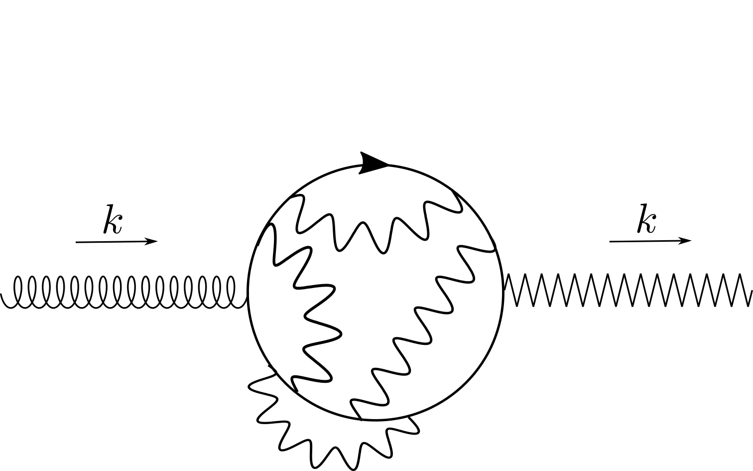
(a) A generic diagram

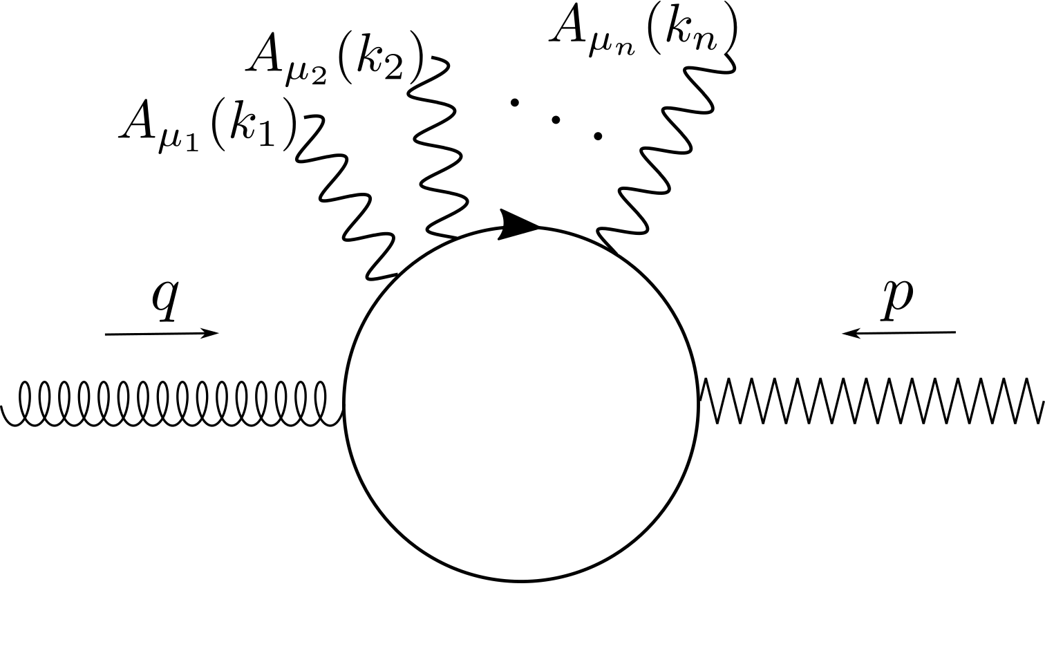
(b) $n$-gauge boson effective vertex

Figure 4.1: (a) A generic diagram for gauge interactions. The internal lines are the gauge fields and the external lines are the stress-energy tensor and the axial current insertions. (b) An $n$ gauge boson effective vertex.

Gauge invariance imposes the following Ward identities:

$$p^{i}\,\Gamma^{(n)}_{ij}(p,\,q,\,k_{1},\dots,\,k_{n})=0,\quad q^{i}\,\Gamma^{(n)}_{ij}(p,\,q,\,k_{1},\dots,\,k_{n})=0.$$ (4.30)

If we differentiate the Ward identities with respect to $p^{r}$ and $q^{r}$ and we then set $p$ and $q$ to zero, we obtain:

$$\Gamma^{(n)}_{ij\mu_{1}\dots\mu_{n}}(0,\,q,\,k_{1},\dots,\,k_{n})=0,\quad\Gamma^{(n)}_{ij\mu_{1}\dots\mu_{n}}(p,\,0,\,k_{1},\dots,\,k_{n})=0;$$

therefore, since these functions are analytic, it follows that

$$\Gamma^{(n)}_{ij\mu_{1}\dots\mu_{n}}(p,\,q,\,k_{1},\dots,\,k_{n})=\mathcal{O}(p),\quad\Gamma^{(n)}_{ij\mu_{1}\dots\mu_{n}}(p,\,k,\,k_{1},\dots,\,k_{n})=\mathcal{O}(k).$$ (4.31)

When $n=0$, for momentum conservation, it must be $q=-p$ and hence

$$\Gamma^{(0)}_{ij\mu_{1}\dots\mu_{n}}(p,\,-p,\,k_{1},\dots,\,k_{n})=\mathcal{O}(p).$$

Instead, when $n>0$ the two momenta are independent and we conclude that

$$\Gamma^{(n)}_{ij\mu_{1}\dots\mu_{n}}(p,\,-p,\,k_{1},\dots,\,k_{n})=\mathcal{O}(pq).$$ (4.32)

Then, if the stress-energy tensor and the axial current are attached to the same fermion loop, the Eq. (4.32) states that the total diagram is $\mathcal{O}(k^{2})$. If instead they are attached to two different loops, we see by using the Eq. (4.31) for each loop, that also these diagrams are $\mathcal{O}(k^{2})$. We would then conclude that only the one-loop free diagram contributes to the AVE (CVE). This argument can be successfully be applied to the chiral vortical effect because electric current is conserved. We conclude that the chiral vortical effect is not affected by radiative corrections.

However, this argument does not apply to AVE because the axial current is not conserved, and consequently, we can not use the first Ward identity in Eq. (4.30). To address the problem, we then split the diagrams into two classes, see Fig. 4.2.

(a) Fermionic stress tensor diagram

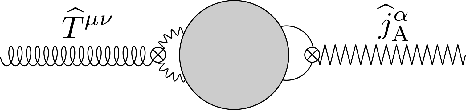
(b) Gauge stress tensor diagram

Figure 4.2: The two diagram classes.

In the first class, Fig. 4.2(a), the stress-energy tensor is connected through the fermionic field. The axial anomaly is captured by the Eq. (4.28). Then, expanding in metric perturbation, the anomaly couples only to the trace of the metric perturbation. Since these diagrams involves the insertion of an off-diagonal component of stress-energy tensor they do not give contribution.

In the second class, Fig. 4.2(b), the stress-energy tensor is connected through the gauge field. Since we proved that in the absence of chiral anomaly no contribution arises for higher orders, the diagrams of this class that actually give contribution are those containing the triangle diagram, which is “responsible” for the chiral anomaly. The generic form of these diagrams are given in Fig. 4.3. The axial current is inserted with the triangle subdiagram and the stress-energy tensor is connected to it through a ladder of box subdiagrams, see Fig. 4.3(b).

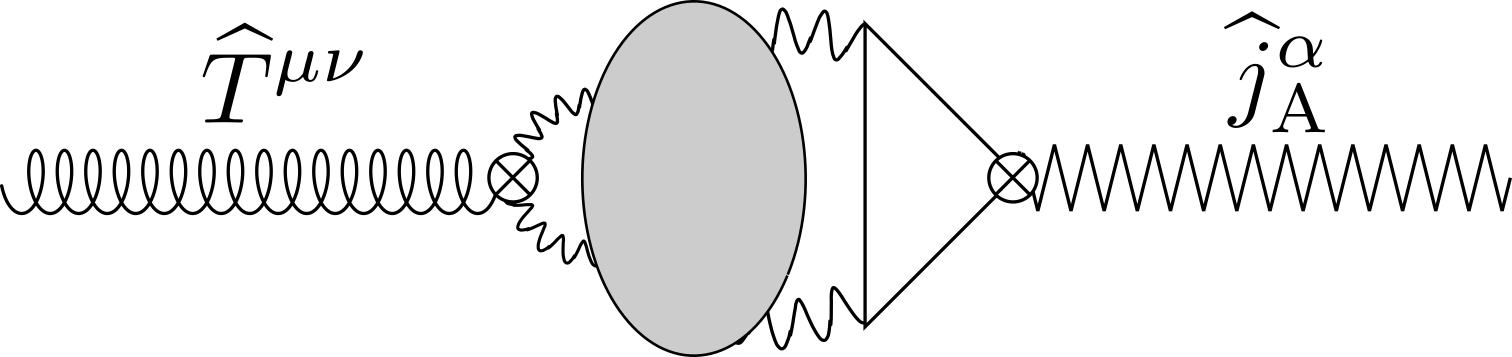
(a) Anomalous diagram

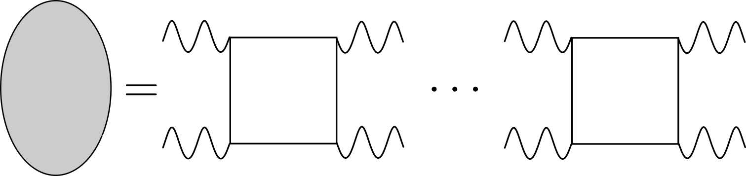
(b) Boxes blob

Figure 4.3: (a) The diagrams that give contribution to the AVE. The blob in (a) is explicitly given in (b) as a ladder of box subdiagrams.

We now proceed to evaluate the two-loop contribution to the AVE using the density matrix formalism. As argued, the first radiative correction comes from the diagram in Fig. 4.4(a). This means that only the gauge part of the stress-energy tensor (4.27) gives corrections to the AVE conductivity.

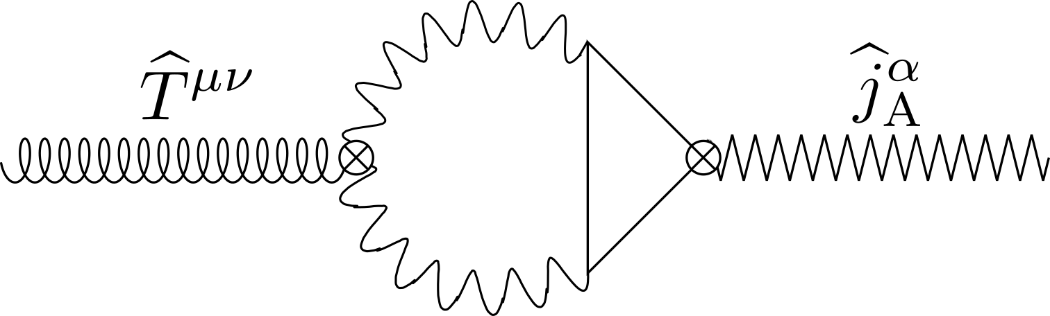
(a) Anomalous diagram

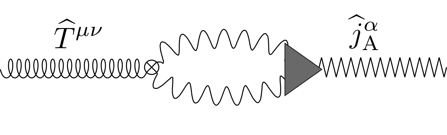
(b) Effective diagram

Figure 4.4: (a) The leading order diagram and (b) the same diagram after replacing the effective vertex, representing the anomalous effect of the triangle diagram.

Moreover, since the triangle part is constrained by the anomalous Ward identity (4.28) we can effectively reduce to one-loop calculation by replacing the triangle part of the diagram with an effective vertex, see Fig. 4.4(b). This effective vertex is captured by replacing the axial current in Eq. (4.29) with the following current

$$\widehat{j}^{\mu}_{\textup{Anom}}=-\frac{e^{2}}{4\pi^{2}}\epsilon^{\mu\nu\lambda\sigma}A_{\nu}\partial_{\lambda}A_{\sigma},$$

which reproduces the chiral anomaly.

To calculate the latter two terms in (4.29) we write the correlation functions in the Euclidean form. Before doing that, we remind the notation:

$$P=(p_{n},{\mathchoice{\mbox{\boldmath$\displaystyle\mathbf{p}$}}{\mbox{\boldmath$\textstyle\mathbf{p}$}}{\mbox{\boldmath$\scriptstyle\mathbf{p}$}}{\mbox{\boldmath$\scriptscriptstyle\mathbf{p}$}}}),\quad X=(\tau,{\mathchoice{\mbox{\boldmath$\displaystyle\mathbf{x}$}}{\mbox{\boldmath$\textstyle\mathbf{x}$}}{\mbox{\boldmath$\scriptstyle\mathbf{x}$}}{\mbox{\boldmath$\scriptscriptstyle\mathbf{x}$}}}),\quad\operatorname*{\mathchoice{\ooalign{$\displaystyle\sum$\cr$\displaystyle\int$\cr}}{\ooalign{\raisebox{0.14pt}{\scalebox{0.7}{$\textstyle\sum$}}\cr$\textstyle\int$\cr}}{\ooalign{\raisebox{0.2pt}{\scalebox{0.6}{$\scriptstyle\sum$}}\cr$\scriptstyle\int$\cr}}{\ooalign{\raisebox{0.2pt}{\scalebox{0.6}{$\scriptstyle\sum$}}\cr$\scriptstyle\int$\cr}}}_{P}=\frac{1}{|\beta|}\sum_{p_{n}=-\infty}^{\infty}\int\frac{\mathrm{d}^{3}p}{(2\pi)^{3}}$$

and:

$$\tilde{\delta}(P)=\int_{0}^{|\beta|}\mathrm{d}\tau\int\mathrm{d}^{3}x\,\mathrm{e}^{{\rm i}X\cdot P}=|\beta|(2\pi)^{3}\delta_{p_{n},0}\,\delta^{(3)}({\mathchoice{\mbox{\boldmath$\displaystyle\mathbf{p}$}}{\mbox{\boldmath$\textstyle\mathbf{p}$}}{\mbox{\boldmath$\scriptstyle\mathbf{p}$}}{\mbox{\boldmath$\scriptscriptstyle\mathbf{p}$}}})$$

where $X\cdot P=\tau\,p_{n}-{\mathchoice{\mbox{\boldmath$\displaystyle\mathbf{x}$}}{\mbox{\boldmath$\textstyle\mathbf{x}$}}{\mbox{\boldmath$\scriptstyle\mathbf{x}$}}{\mbox{\boldmath$\scriptscriptstyle\mathbf{x}$}}}{\mathchoice{\mbox{\boldmath$\displaystyle\mathbf{p}$}}{\mbox{\boldmath$\textstyle\mathbf{p}$}}{\mbox{\boldmath$\scriptstyle\mathbf{p}$}}{\mbox{\boldmath$\scriptscriptstyle\mathbf{p}$}}}$ and $p_{n}=2\pi n/|\beta|$ are the bosonic Matsubara frequencies. The photon propagator, see Eq. (2.9), in the imaginary time reads:

$$\langle{\rm T}_{\tau}A_{\mu}(X)A_{\nu}(Y)\rangle_{T}=\operatorname*{\mathchoice{\ooalign{$\displaystyle\sum$\cr$\displaystyle\int$\cr}}{\ooalign{\raisebox{0.14pt}{\scalebox{0.7}{$\textstyle\sum$}}\cr$\textstyle\int$\cr}}{\ooalign{\raisebox{0.2pt}{\scalebox{0.6}{$\scriptstyle\sum$}}\cr$\scriptstyle\int$\cr}}{\ooalign{\raisebox{0.2pt}{\scalebox{0.6}{$\scriptstyle\sum$}}\cr$\scriptstyle\int$\cr}}}_{P}\mathrm{e}^{{\rm i}P(X-Y)}\frac{G_{\mu\nu}(P)}{P^{2}}$$ (4.33)

where:

$$G_{\mu\nu}(P)=\delta_{\mu,\nu}+(1-\xi)\frac{P_{\mu}P_{\nu}}{P^{2}}$$

and $P^{2}$ is the Euclidean squared magnitude of the four vector $P$.

The Euclidean effective axial current using the point splitting procedure (see Sec. 2.4.2) reads:

$$\begin{split}\widehat{j}&{}_{\textup{Anom}}^{\alpha}(X)=-\frac{e^{2}}{4\pi^{2}}\epsilon^{\alpha\nu\lambda\sigma}A_{\nu}(X)\partial_{\lambda}A_{\sigma}(X)\\ &=\lim_{X_{1},X_{2}\to X}\frac{e^{2}}{8\pi^{2}}\epsilon^{\alpha\rho\lambda\tau}(\partial_{X_{1}\lambda}-\partial_{X_{2}\lambda})A_{\rho}(X_{1})A_{\tau}(X_{2})\\ &\equiv\mathcal{J}_{\textup{Anom}}^{\alpha,\,\rho\tau}(\partial_{X_{1}},\partial_{X_{2}})A_{\rho}(X_{1})A_{\tau}(X_{2}).\end{split}$$

Instead the electromagnetic stress-energy tensor is

$$\widehat{T}_{\textup{em}}^{\mu\nu}(X)=\lim_{X_{1},X_{2}\to X}\mathcal{D}_{\textup{em}}^{\mu\nu,\,\kappa\sigma}(\partial_{X_{1}},\partial_{X_{2}})A_{\kappa}(X_{1})A_{\sigma}(X_{2})$$

with

$$\begin{split}\mathcal{D}_{\textup{em}}^{\mu\nu,\,\kappa\sigma}(\partial_{X_{1}},\partial_{X_{2}})=\frac{1}{2}\Big{[}&\delta^{\kappa,\sigma}\!\left(\partial^{\mu}_{X_{1}}\partial^{\nu}_{X_{2}}\!+\!\partial^{\nu}_{X_{1}}\partial^{\mu}_{X_{2}}\right)-\!\left(\delta^{\sigma,\nu}\partial^{\mu}_{X_{1}}\partial^{\kappa}_{X_{2}}+\delta^{\kappa,\nu}\partial^{\sigma}_{X_{1}}\partial^{\mu}_{X_{2}}\right)\\ &\!-\!\left(\delta^{\kappa,\mu}\partial^{\sigma}_{X_{1}}\partial^{\nu}_{X_{2}}\!+\!\delta^{\sigma,\mu}\partial^{\nu}_{X_{1}}\partial^{\kappa}_{X_{2}}\right)+\left(\delta^{\kappa,\mu}\delta^{\sigma,\nu}\!+\!\delta^{\kappa,\nu}\delta^{\sigma,\mu}\right)\partial_{X_{1}}\!\!\!\cdot\!\partial_{X_{2}}\\ &\!\!-\!\eta^{\mu\nu}\!\left(\delta^{\kappa,\sigma}\partial_{X_{1}}\!\!\!\cdot\!\partial_{X_{2}}\!-\!\partial^{\sigma}_{X_{1}}\partial^{\kappa}_{X_{2}}\right)\Big{]}.\end{split}$$

Now we are ready to evaluate the two-loop correction of the coefficient from Eq. (4.29)

$$C_{\mu\nu\alpha i}^{\textup{A}}=\int_{0}^{|\beta|}\mathrm{d}\tau\int\mathrm{d}^{3}x\langle\widehat{T}^{\mu\nu}(X)\widehat{j}^{\,\alpha}_{\textup{A}}(0)\rangle_{T,c}x^{i}.$$ (4.34)

First, we consider:

$$\begin{split}\langle{\rm T}_{\tau}\widehat{T}^{\mu\nu}(X)\widehat{j}_{\textup{Anom}}^{\alpha}(Y)\rangle_{T,c}=&\lim_{\begin{subarray}{c}X_{1},X_{2}\to X\\ Y_{1},Y_{2}\to Y\end{subarray}}\mathcal{D}_{\textup{em}}^{\mu\nu,\,\kappa\sigma}(\partial_{X_{1}},\partial_{X_{2}})\times\\ &\times\mathcal{J}_{\textup{Anom}}^{\alpha,\,\rho\tau}(\partial_{Y_{1}},\partial_{Y_{2}})\langle{\rm T}_{\tau}A_{\kappa}(X_{1})A_{\sigma}(X_{2})A_{\rho}(Y_{1})A_{\tau}(Y_{2})\rangle_{T,c}.\end{split}$$

The evaluation of the four gauge field correlator can be done by employing the standard Wick theorem and since only its connected part appears, only the following two terms survive:

$$\begin{split}\langle A_{1}A_{2}A_{3}A_{4}\rangle_{c}&=\langle A_{1}A_{2}A_{3}A_{4}\rangle-\langle A_{1}A_{2}\rangle\langle A_{3}A_{4}\rangle\\ &=\langle A_{1}A_{3}\rangle\langle A_{2}A_{4}\rangle+\langle A_{1}A_{4}\rangle\langle A_{2}A_{3}\rangle.\end{split}$$

It can be shown that these two latters terms give the same contribution, therefore we consider just the first one. The only correlators left are the already known two point correlators of the photon; in the Fourier space we can choose the following notation to express them as in (4.33)

$$\langle{\rm T}_{\tau}A_{\kappa}(X_{1})A_{\rho}(Y_{1})\rangle_{T}=\operatorname*{\mathchoice{\ooalign{$\displaystyle\sum$\cr$\displaystyle\int$\cr}}{\ooalign{\raisebox{0.14pt}{\scalebox{0.7}{$\textstyle\sum$}}\cr$\textstyle\int$\cr}}{\ooalign{\raisebox{0.2pt}{\scalebox{0.6}{$\scriptstyle\sum$}}\cr$\scriptstyle\int$\cr}}{\ooalign{\raisebox{0.2pt}{\scalebox{0.6}{$\scriptstyle\sum$}}\cr$\scriptstyle\int$\cr}}}_{P}\mathrm{e}^{{\rm i}P(X_{1}-Y_{1})}\frac{G_{\kappa\rho}(P)}{P^{2}},$$

$$\langle{\rm T}_{\tau}A_{\sigma}(X_{2})A_{\tau}(Y_{2})\rangle_{T}=\operatorname*{\mathchoice{\ooalign{$\displaystyle\sum$\cr$\displaystyle\int$\cr}}{\ooalign{\raisebox{0.14pt}{\scalebox{0.7}{$\textstyle\sum$}}\cr$\textstyle\int$\cr}}{\ooalign{\raisebox{0.2pt}{\scalebox{0.6}{$\scriptstyle\sum$}}\cr$\scriptstyle\int$\cr}}{\ooalign{\raisebox{0.2pt}{\scalebox{0.6}{$\scriptstyle\sum$}}\cr$\scriptstyle\int$\cr}}}_{Q}\mathrm{e}^{{\rm i}Q(X_{2}-Y_{2})}\frac{G_{\sigma\tau}(Q)}{Q^{2}}.$$

Since the coordinate dependence is now only in the exponential factor, the derivative action present in the operators $\mathcal{D}_{\textup{em}}$ and $\mathcal{J}_{\textup{Anom}}$ is easily found:

$$\partial_{X}\langle{\rm T}_{\tau}A_{\mu}(X)A_{\nu}(Y)\rangle_{T}={\rm i}P\langle{\rm T}_{\tau}A_{\mu}(X)A_{\nu}(Y)\rangle_{T};$$

$$\partial_{Y}\langle{\rm T}_{\tau}A_{\mu}(X)A_{\nu}(Y)\rangle_{T}=-{\rm i}P\langle{\rm T}_{\tau}A_{\mu}(X)A_{\nu}(Y)\rangle_{T}.$$

With these substitutions and after the limit of $X_{1},X_{2}\to X$ and $Y_{1},Y_{2}\to Y$ the correlator in $Y=0$ becomes

$$\begin{split}\langle{\rm T}_{\tau}&\widehat{T}^{\mu\nu}(X)\widehat{j}_{\textup{Anom}}^{\alpha}(0)\rangle_{T,c}=\operatorname*{\mathchoice{\ooalign{$\displaystyle\sum$\cr$\displaystyle\int$\cr}}{\ooalign{\raisebox{0.14pt}{\scalebox{0.7}{$\textstyle\sum$}}\cr$\textstyle\int$\cr}}{\ooalign{\raisebox{0.2pt}{\scalebox{0.6}{$\scriptstyle\sum$}}\cr$\scriptstyle\int$\cr}}{\ooalign{\raisebox{0.2pt}{\scalebox{0.6}{$\scriptstyle\sum$}}\cr$\scriptstyle\int$\cr}}}_{P,Q}\frac{F^{\mu\nu\alpha}(P,Q)}{P^{2}Q^{2}}\mathrm{e}^{{\rm i}(P+Q)\cdot X},\end{split}$$

where the function $F^{\mu\nu\alpha}$ results from the composite operator in the correlation functions, in this case:

$$\begin{split}F^{\mu\nu\alpha}(P,Q)=&2\,\mathcal{D}_{\textup{em}}^{\mu\nu,\,\kappa\sigma}({\rm i}P,{\rm i}Q)\mathcal{J}_{\textup{Anom}}^{\alpha,\,\rho\tau}(-{\rm i}Q,-{\rm i}P)G_{\kappa\rho}(P)G_{\sigma\tau}(Q)\\ =&\frac{{\rm i}e^{2}}{8\pi^{2}}\left[\left(P_{\mu}-Q_{\mu}\right)\epsilon_{\alpha\nu\rho\sigma}P_{\rho}Q_{\sigma}+\left(P_{\nu}-Q_{\nu}\right)\epsilon_{\alpha\mu\rho\sigma}P_{\rho}Q_{\sigma}\right].\end{split}$$ (4.35)

So the coefficient (4.34) becomes

$$C^{\textup{A}}_{\mu\nu\alpha i}=\int_{0}^{|\beta|}\frac{\mathrm{d}\tau}{|\beta|}\int\mathrm{d}^{3}x\operatorname*{\mathchoice{\ooalign{$\displaystyle\sum$\cr$\displaystyle\int$\cr}}{\ooalign{\raisebox{0.14pt}{\scalebox{0.7}{$\textstyle\sum$}}\cr$\textstyle\int$\cr}}{\ooalign{\raisebox{0.2pt}{\scalebox{0.6}{$\scriptstyle\sum$}}\cr$\scriptstyle\int$\cr}}{\ooalign{\raisebox{0.2pt}{\scalebox{0.6}{$\scriptstyle\sum$}}\cr$\scriptstyle\int$\cr}}}_{P,Q}\mathrm{e}^{{\rm i}(P+Q)X}x_{i}\frac{F_{\mu\nu\alpha}(P,Q)}{P^{2}Q^{2}}$$

and rewriting the coordinate $x_{i}$ as derivative of the exponential and integrating by part

$$\begin{split}C^{\textup{A}}_{\mu\nu\alpha i}&=-{\rm i}\int_{0}^{|\beta|}\frac{\mathrm{d}\tau}{|\beta|}\int\mathrm{d}^{3}x\operatorname*{\mathchoice{\ooalign{$\displaystyle\sum$\cr$\displaystyle\int$\cr}}{\ooalign{\raisebox{0.14pt}{\scalebox{0.7}{$\textstyle\sum$}}\cr$\textstyle\int$\cr}}{\ooalign{\raisebox{0.2pt}{\scalebox{0.6}{$\scriptstyle\sum$}}\cr$\scriptstyle\int$\cr}}{\ooalign{\raisebox{0.2pt}{\scalebox{0.6}{$\scriptstyle\sum$}}\cr$\scriptstyle\int$\cr}}}_{P,Q}\left(\frac{\partial}{\partial q^{i}}\mathrm{e}^{{\rm i}(P+Q)X}\right)\frac{F_{\mu\nu\alpha}(P,Q)}{P^{2}Q^{2}}\\ &={\rm i}\!\operatorname*{\mathchoice{\ooalign{$\displaystyle\sum$\cr$\displaystyle\int$\cr}}{\ooalign{\raisebox{0.14pt}{\scalebox{0.7}{$\textstyle\sum$}}\cr$\textstyle\int$\cr}}{\ooalign{\raisebox{0.2pt}{\scalebox{0.6}{$\scriptstyle\sum$}}\cr$\scriptstyle\int$\cr}}{\ooalign{\raisebox{0.2pt}{\scalebox{0.6}{$\scriptstyle\sum$}}\cr$\scriptstyle\int$\cr}}}_{P,Q}\!\int_{0}^{|\beta|}\frac{\mathrm{d}\tau}{|\beta|}\int\mathrm{d}^{3}x\,\mathrm{e}^{{\rm i}(P+Q)X}\!\!\left(\frac{\partial}{\partial q^{i}}\frac{F_{\mu\nu\alpha}(P,Q)}{P^{2}Q^{2}}\right).\end{split}$$

At this point, the integral over the coordinates gives a $\tilde{\delta}(P+Q)$, that we can use to sum over the momentum $Q$

$$C^{\textup{A}}_{\mu\nu\alpha i}=\frac{{\rm i}}{|\beta|}\operatorname*{\mathchoice{\ooalign{$\displaystyle\sum$\cr$\displaystyle\int$\cr}}{\ooalign{\raisebox{0.14pt}{\scalebox{0.7}{$\textstyle\sum$}}\cr$\textstyle\int$\cr}}{\ooalign{\raisebox{0.2pt}{\scalebox{0.6}{$\scriptstyle\sum$}}\cr$\scriptstyle\int$\cr}}{\ooalign{\raisebox{0.2pt}{\scalebox{0.6}{$\scriptstyle\sum$}}\cr$\scriptstyle\int$\cr}}}_{P}\left(\frac{\partial}{\partial q^{i}}\frac{F_{\mu\nu\alpha}(P,Q)}{P^{2}Q^{2}}\right)_{Q=-P}.$$

The derivative of the quantity in the bracket is simplified by the property $F_{\mu\nu\alpha}(P,-P)=0$, as we see from (4.35):

$$\begin{split}\left(\frac{\partial}{\partial q^{i}}\frac{F_{\mu\nu\alpha}(P,Q)}{P^{2}Q^{2}}\right)_{Q=-P}&=\frac{1}{P^{4}}\left(\frac{\partial}{\partial q^{i}}F_{\mu\nu\alpha}(P,Q)\right)_{Q=-P}\\ &\equiv\frac{f_{\mu\nu\alpha i}(p_{n},\mathchoice{\mbox{\boldmath$\displaystyle\mathbf{p}$}}{\mbox{\boldmath$\textstyle\mathbf{p}$}}{\mbox{\boldmath$\scriptstyle\mathbf{p}$}}{\mbox{\boldmath$\scriptscriptstyle\mathbf{p}$}})}{(p_{n}^{2}+{\mathchoice{\mbox{\boldmath$\displaystyle\mathbf{p}$}}{\mbox{\boldmath$\textstyle\mathbf{p}$}}{\mbox{\boldmath$\scriptstyle\mathbf{p}$}}{\mbox{\boldmath$\scriptscriptstyle\mathbf{p}$}}}^{2})^{2}},\end{split}$$

where we have defined the function $f_{\mu\nu\alpha i}(p_{n},\mathchoice{\mbox{\boldmath$\displaystyle\mathbf{p}$}}{\mbox{\boldmath$\textstyle\mathbf{p}$}}{\mbox{\boldmath$\scriptstyle\mathbf{p}$}}{\mbox{\boldmath$\scriptscriptstyle\mathbf{p}$}})$, which is a polynomial function. For instance we need

$$f_{0132}=\frac{{\rm i}e^{2}}{4\pi^{2}}(p_{n}^{2}-{p^{1}}^{2}),\quad f_{0231}=-\frac{{\rm i}e^{2}}{4\pi^{2}}(p_{n}^{2}-{p^{2}}^{2}).$$

We are then reduced to a single momentum integral that can be made explicitly with standard technique. Consider first

$$\begin{split}C^{\textup{A}}_{0132}&=-\frac{e^{2}}{4\pi^{2}|\beta|}\int\mathrm{d}p\frac{1}{|\beta|}\sum_{p_{n}}\int_{4\pi}\frac{\mathrm{d}\Omega_{p}}{(2\pi)^{3}}\frac{p^{2}(p_{n}^{2}-p_{1}^{2})}{(p_{n}^{2}+{\mathchoice{\mbox{\boldmath$\displaystyle\mathbf{p}$}}{\mbox{\boldmath$\textstyle\mathbf{p}$}}{\mbox{\boldmath$\scriptstyle\mathbf{p}$}}{\mbox{\boldmath$\scriptscriptstyle\mathbf{p}$}}}^{2})^{2}}\\ &=-\frac{e^{2}}{8\pi^{4}|\beta|}\int\mathrm{d}p\frac{1}{|\beta|}\sum_{p_{n}}\frac{p^{2}(p_{n}^{2}-p^{2}/3)}{(p_{n}^{2}+{\mathchoice{\mbox{\boldmath$\displaystyle\mathbf{p}$}}{\mbox{\boldmath$\textstyle\mathbf{p}$}}{\mbox{\boldmath$\scriptstyle\mathbf{p}$}}{\mbox{\boldmath$\scriptscriptstyle\mathbf{p}$}}}^{2})^{2}}\\ &=-\frac{e^{2}}{24\pi^{4}|\beta|}\int\mathrm{d}p\left(p\,n_{\textup{B}}(p)+2p^{2}n_{\textup{B}}^{\prime}(p)\right),\end{split}$$

where $n_{\textup{B}}$ is the Bose-Einstein distribution function

$$n_{\textup{B}}(p)=\frac{1}{\mathrm{e}^{|\beta|p}-1}$$

and $n_{\textup{B}}^{\prime}(p)$ its derivative that can be integrated by parts:

$$\int\mathrm{d}p\,2p^{2}\,n_{\textup{B}}^{\prime}(p)=-4\int\mathrm{d}p\,p\,n_{\textup{B}}(p).$$

At the end we are left with

$$\begin{split}C^{\textup{A}}_{0132}&=\frac{e^{2}}{8\pi^{4}|\beta|}\int\mathrm{d}p\,p\,n_{\textup{B}}(p)=\frac{e^{2}}{48\pi^{2}}T^{3}.\end{split}$$

In the same way we can show that $C^{\textup{A}}_{0231}=-C^{\textup{A}}_{0132}$ so that the two-loop correction of (4.29) is

$$W^{\textup{A}}_{(2)}=\frac{e^{2}}{24\pi^{2}}T^{3}.$$ (4.36)

Our result is twice the value of [24, 66] because we have considered both right and left fermions contribution instead that just one chirality. We have then explicitly shown a radiative correction of AVE. Notice that this term is compatible with the constraint we have found for this conductivity:

$$\left(3+|\beta|\frac{\partial}{\partial\beta}\right)W^{\textup{A}}=0.$$

This result is also easily generalized to a QCD like non-Abelian gauge theory with $N_{c}$ colors and $N_{f}$ flavors, we obtain

$$W^{\textup{A}}=N_{c}N_{f}\left(\frac{\zeta_{\textup{A}}^{2}T^{3}}{2\pi^{2}}+\frac{T^{3}}{6}+\frac{N_{c}^{2}-1}{2N_{c}}\frac{g_{0}^{2}}{24\pi^{2}}T^{3}\right),$$

where $g_{0}$ is the Yang-Mills coupling. This kinds of corrections could play a significant role in the phenomenology of the Quark-Gluon Plasma, where thanks to the strong coupling this effect could be enhanced. It would be particularly important to address the case of massive fields. Because if it turns out that this correction is also proportional to the naive chiral anomaly, then the intensity of this correction can be estimated in the order of the pion mass squared. Indeed, using the partial conservation of axial current the naive chiral anomaly is

$$\partial_{\mu}\widehat{j}^{\mu}_{\textup{A}}=F_{\pi}m_{\pi}^{2}\pi^{0},$$

where $F_{\pi}$ is the pion decay constant, $m_{\pi}$ the pion mass, and $\pi^{0}$ the pion field.

Conclusions

The present thesis aimed to examine the effects of vorticity on the thermodynamics of relativistic quantum systems. The main goal of the current study was to determine a theoretical framework to address quantum effects induced by vorticity, keeping full covariant and quantum properties of the system. In particular, since a complete quantum regime could hinder a kinetic theory, the method proposed does not rely on it.

The second aim of this study was to investigate the effects of vorticity in the presence of chiral matter and external electromagnetic field. To that objective, this work has been focused on systems consisting of massless chiral fermions. For those systems, this thesis had the purpose of determining and examining quantum thermodynamics phenomena induced by chirality, vorticity and magnetic field.

This thesis has identified in Zubarev’s non-equilibrium statistical operator the quantitative framework for detecting the effects of thermal vorticity on relativistic quantum systems. This study has also shown that Zubarev’s method can be reliably used to study global thermal equilibrium in the mutual presence of thermal vorticity, chirality and external electromagnetic field. The analysis has shown that the usual ideal thermodynamics is to be changed in the presence of thermal vorticity. This method also recovered the significant quantum phenomena known in the literature, namely the chiral magnetic effect, the chiral vortical effect, the axial vortical effect and the chiral separation effect. The investigation of constitutive equations has also revealed the presence of additional effects at second-order on thermal vorticity. This thesis has provided a deeper insight into the interconnection between spin, chirality and vorticity; for instance, it showed the relations between expectation values of spin tensor and axial current.

This study has also identified and presented the exact solutions of thermal states for a system at global thermal equilibrium consisting of chiral massless fermions under the action of an external constant homogeneous magnetic field. Taking advantage of these exact solutions and conservation equations, the study also proved that the thermal coefficients related to first-order effects on thermal vorticity do not receive corrections from the external electromagnetic field. The same argument revealed existing relations between those thermal coefficients, even connecting coefficients related to vorticity to other related to electromagnetic field. For instance, this analysis has found that the chiral vortical effect and the chiral magnetic effect conductivities are connected one to the other by a differential equation. Therefore, this research provides insights into the relations between the effects and the interplay of electromagnetic fields and vorticity.

One of the more significant findings to emerge from this study is that the axial vortical effect is not entirely dictated by the chiral anomaly or by other types of quantum anomalies. Indeed, the origination of the axial vortical effect is explained by just the symmetries of the statistical operator. The results of this investigation support this view by showing that, for massive fields, any relations with quantum anomalies are lost. As additional evidence, a Coleman-Hill-like argument revealed that the axial vortical effect conductivity is not protected against radiative corrections. This fact clearly indicated that quantum anomalies could not cause the effects, because non-renormalization theorems should instead protect them. The explicit calculation of the first-order corrections, made with Zubarev’s methods, is in agreement with previous predictions.

Appendix A Useful resources

A.1 Summary of $\mathsf{P}$, $\mathsf{T}$ and $\mathsf{C}$ transformations

We report transformation parities of various operators relevant for hydrodynamics and of operators built with Dirac algebra. We indicate with $\mathsf{P},\,\mathsf{T},\,\mathsf{C}$ respectively parity, time reversal and charge conjugation transformations. While $\widehat{T},\widehat{j}_{\textup{V}},\widehat{j}_{\textup{A}},\widehat{S}$ are the stress-energy tensor, vector current, axial current and spin operators, $\widehat{\psi}$ is Dirac field and $\widehat{\sigma}^{\mu\nu}=\widehat{\bar{\psi}}[\gamma^{\mu},\gamma^{\nu}]\widehat{\psi}$. In the local rest frame of thermal bath $u=(1,\mathchoice{\mbox{\boldmath$\displaystyle\mathbf{0}$}}{\mbox{\boldmath$\textstyle\mathbf{0}$}}{\mbox{\boldmath$\scriptstyle\mathbf{0}$}}{\mbox{\boldmath$\scriptscriptstyle\mathbf{0}$}})$ the previous quantities transform as follow:

$$\begin{array}[]{lccc|ccccccccccc}&\widehat{T}_{00}&\widehat{T}_{0i}&\widehat{T}_{ij}&\widehat{j}^{0}_{\textup{V}}&\widehat{\mathchoice{\mbox{\boldmath$\displaystyle\mathbf{j}$}}{\mbox{\boldmath$\textstyle\mathbf{j}$}}{\mbox{\boldmath$\scriptstyle\mathbf{j}$}}{\mbox{\boldmath$\scriptscriptstyle\mathbf{j}$}}}_{\textup{V}}&\widehat{j}^{0}_{\textup{A}}&\widehat{\mathchoice{\mbox{\boldmath$\displaystyle\mathbf{j}$}}{\mbox{\boldmath$\textstyle\mathbf{j}$}}{\mbox{\boldmath$\scriptstyle\mathbf{j}$}}{\mbox{\boldmath$\scriptscriptstyle\mathbf{j}$}}}_{\textup{A}}&\widehat{\sigma}^{0i}&\widehat{\sigma}^{ij}&\widehat{\bar{\psi}}\widehat{\psi}&{\rm i}\widehat{\bar{\psi}}\gamma^{5}\widehat{\psi}&\widehat{S}^{0,ij}&\widehat{S}^{i,0j}&\widehat{S}^{i,jk}\\ \hline\cr\mathsf{P}&+&-&+&+&-&-&+&-&+&+&-&+&+&-\\ \mathsf{T}&+&-&+&+&-&+&-&+&-&+&-&\pm&\pm&\pm\\ \mathsf{C}&+&+&+&-&-&+&+&-&-&+&+&+&+&+\\ \end{array}$$ (A.1)

Consider then the inverse four-temperature $\beta$, the thermal vorticity tensor $\varpi$ and for an electromagnetic field, the gauge potential $A$, the electric field $E$ and the magnetic field $B$. We indicate with $\widehat{\mathchoice{\mbox{\boldmath$\displaystyle\mathbf{K}$}}{\mbox{\boldmath$\textstyle\mathbf{K}$}}{\mbox{\boldmath$\scriptstyle\mathbf{K}$}}{\mbox{\boldmath$\scriptscriptstyle\mathbf{K}$}}}$ and $\widehat{\mathchoice{\mbox{\boldmath$\displaystyle\mathbf{J}$}}{\mbox{\boldmath$\textstyle\mathbf{J}$}}{\mbox{\boldmath$\scriptstyle\mathbf{J}$}}{\mbox{\boldmath$\scriptscriptstyle\mathbf{J}$}}}$, respectively the boosts and rotations generators. $\widehat{Q}$ is electric charge operator, $\widehat{Q}_{\textup{A}}$ is axial charge operator and $\widehat{\rho}$ is the statistical operator with both conserved vector and axial currents. Those quantities transform as follow

$$\begin{array}[]{lcccc|cccc|cccc|ccccc}&\beta_{0}&\mathchoice{\mbox{\boldmath$\displaystyle\mathbf{\beta}$}}{\mbox{\boldmath$\textstyle\mathbf{\beta}$}}{\mbox{\boldmath$\scriptstyle\mathbf{\beta}$}}{\mbox{\boldmath$\scriptscriptstyle\mathbf{\beta}$}}&\varpi_{i0}&\varpi_{ij}&A_{0}&\mathchoice{\mbox{\boldmath$\displaystyle\mathbf{A}$}}{\mbox{\boldmath$\textstyle\mathbf{A}$}}{\mbox{\boldmath$\scriptstyle\mathbf{A}$}}{\mbox{\boldmath$\scriptscriptstyle\mathbf{A}$}}&\mathchoice{\mbox{\boldmath$\displaystyle\mathbf{E}$}}{\mbox{\boldmath$\textstyle\mathbf{E}$}}{\mbox{\boldmath$\scriptstyle\mathbf{E}$}}{\mbox{\boldmath$\scriptscriptstyle\mathbf{E}$}}&\mathchoice{\mbox{\boldmath$\displaystyle\mathbf{B}$}}{\mbox{\boldmath$\textstyle\mathbf{B}$}}{\mbox{\boldmath$\scriptstyle\mathbf{B}$}}{\mbox{\boldmath$\scriptscriptstyle\mathbf{B}$}}&\widehat{\mathchoice{\mbox{\boldmath$\displaystyle\mathbf{K}$}}{\mbox{\boldmath$\textstyle\mathbf{K}$}}{\mbox{\boldmath$\scriptstyle\mathbf{K}$}}{\mbox{\boldmath$\scriptscriptstyle\mathbf{K}$}}}&\widehat{\mathchoice{\mbox{\boldmath$\displaystyle\mathbf{J}$}}{\mbox{\boldmath$\textstyle\mathbf{J}$}}{\mbox{\boldmath$\scriptstyle\mathbf{J}$}}{\mbox{\boldmath$\scriptscriptstyle\mathbf{J}$}}}&(\widehat{K}\widehat{K},\,\widehat{J}\widehat{J})&\widehat{K}\widehat{J}&\mu&\widehat{Q}&\mu_{5}&\widehat{Q}_{\textup{A}}&\widehat{\rho}\\ \hline\cr\mathsf{P}&+&-&-&+&+&-&-&+&-&+&+&-&+&+&-&-&\pm\\ \mathsf{T}&+&-&+&-&+&-&+&-&+&-&+&-&+&+&+&+&+\\ \mathsf{C}&+&+&+&+&-&-&-&-&+&+&+&+&-&-&+&+&\pm\\ \end{array}$$ (A.2)

where with $\pm$ we indicate that it does not simply acquires a phase but transformation is more complex. From the inverse four-temperature and thermal vorticity $\varpi$ we can construct a tetrad $\{\beta,\alpha,w,\gamma\}$, which transform as following

$$\begin{array}[]{lcccccccc}&\beta_{0}&\mathchoice{\mbox{\boldmath$\displaystyle\mathbf{\beta}$}}{\mbox{\boldmath$\textstyle\mathbf{\beta}$}}{\mbox{\boldmath$\scriptstyle\mathbf{\beta}$}}{\mbox{\boldmath$\scriptscriptstyle\mathbf{\beta}$}}&\alpha_{0}&\mathchoice{\mbox{\boldmath$\displaystyle\mathbf{\alpha}$}}{\mbox{\boldmath$\textstyle\mathbf{\alpha}$}}{\mbox{\boldmath$\scriptstyle\mathbf{\alpha}$}}{\mbox{\boldmath$\scriptscriptstyle\mathbf{\alpha}$}}&w_{0}&\mathchoice{\mbox{\boldmath$\displaystyle\mathbf{w}$}}{\mbox{\boldmath$\textstyle\mathbf{w}$}}{\mbox{\boldmath$\scriptstyle\mathbf{w}$}}{\mbox{\boldmath$\scriptscriptstyle\mathbf{w}$}}&\gamma_{0}&\mathchoice{\mbox{\boldmath$\displaystyle\mathbf{\gamma}$}}{\mbox{\boldmath$\textstyle\mathbf{\gamma}$}}{\mbox{\boldmath$\scriptstyle\mathbf{\gamma}$}}{\mbox{\boldmath$\scriptscriptstyle\mathbf{\gamma}$}}\\ \hline\cr\mathsf{P}&+&-&+&-&-&+&+&-\\ \mathsf{T}&+&-&-&+&+&-&+&-\\ \mathsf{C}&+&+&+&+&+&+&+&+\\ \end{array}$$ (A.3)

A.2 Thermodynamic relations in $\beta$ frame

At global thermal equilibrium with vorticity, thermodynamic fields satisfy several equilibrium relations which constraints their coordinate dependence. In the $\beta$-frame, we can build several quantities from the four-vector $\beta$ and thermal vorticity $\varpi$:

$$u_{\mu}=\frac{\beta_{\mu}}{\sqrt{\beta^{2}}};\quad\Delta^{\mu\nu}=g^{\mu\nu}-u^{\mu}u^{\nu};\quad\varpi_{\mu\nu}=\partial_{\nu}\beta_{\mu}=\epsilon_{\mu\nu\rho\sigma}w^{\rho}u^{\sigma}+\alpha_{\mu}u_{\nu}-\alpha_{\nu}u_{\mu};$$

$$\alpha_{\mu}=\varpi_{\mu\nu}u^{\nu};\quad w_{\mu}=-\frac{1}{2}\epsilon_{\mu\nu\rho\sigma}\varpi^{\nu\rho}u^{\sigma};\quad\gamma_{\mu}=(\alpha\cdot\varpi)^{\lambda}\Delta_{\lambda\mu}=\epsilon_{\mu\nu\rho\sigma}w^{\nu}\alpha^{\rho}u^{\sigma}.$$

Most of these quantities depend on coordinates and their derivatives are [46]:

$$\partial_{\nu}\beta_{\mu}=\varpi_{\mu\nu};\quad\partial_{\nu}=-\alpha_{\nu}\frac{\partial}{\partial\sqrt{\beta^{2}}};\quad\varpi:\varpi=2\left(\alpha^{2}-w^{2}\right)$$

$$\partial_{\nu}u_{\mu}=\frac{1}{\sqrt{\beta^{2}}}\big{(}\varpi_{\mu\nu}+\alpha_{\nu}u_{\mu}\big{)};\quad\partial^{\alpha}u_{\alpha}=0;\quad u_{\alpha}\partial^{\alpha}u_{\mu}=\frac{\alpha_{\mu}}{\sqrt{\beta^{2}}};$$

$$\partial_{\mu}\alpha_{\nu}=\frac{1}{\sqrt{\beta^{2}}}\big{(}\varpi_{\nu\rho}\varpi^{\rho}_{\;\mu}+\alpha_{\mu}\alpha_{\nu}\big{)};\quad\partial^{\alpha}\alpha_{\alpha}=\frac{1}{\sqrt{\beta^{2}}}\big{(}2w^{2}-\alpha^{2}\big{)};\quad u_{\alpha}\partial^{\alpha}\alpha^{2}=0;$$

$$\partial_{\mu}w_{\nu}=\frac{1}{\sqrt{\beta^{2}}}\big{(}\alpha_{\mu}w_{\nu}-\frac{1}{2}\epsilon_{\nu\rho\sigma\lambda}\varpi^{\rho\sigma}\varpi^{\lambda}_{\;\mu}\big{)};\quad\partial^{\alpha}w_{\alpha}=-3\frac{w\cdot\alpha}{\sqrt{\beta^{2}}};\quad u_{\alpha}\partial^{\alpha}w^{2}=0;$$

$$\alpha^{\sigma}\partial_{\mu}\alpha_{\sigma}=w^{\sigma}\partial_{\mu}w_{\sigma}=\frac{1}{\sqrt{\beta^{2}}}\big{(}w^{2}\alpha_{\mu}-(\alpha\cdot w)w_{\mu}\big{)};\quad\partial_{\mu}(\alpha\cdot w)=0;$$

$$\partial_{\alpha}\gamma^{\alpha}=0;\quad\partial^{\alpha}\Delta_{\alpha\beta}=-\frac{\alpha_{\beta}}{\sqrt{\beta^{2}}}.$$

A.3 Identities for massless momentum integrals

The integrals in thermodynamics quantities related to massless fermions can be turn into the general integral:

$$\begin{split}\int_{0}^{\infty}\mathrm{d}p\,p^{k}\left(\frac{1}{\mathrm{e}^{|\beta|(p-\mu)}+1}+\frac{1}{\mathrm{e}^{|\beta|(p-\mu)}+1}\right)=&-|\beta|^{-k-1}k\,\Gamma(k)\times\\ &\times\left(\mathrm{Li}_{k+1}(-\mathrm{e}^{|\beta|\mu})+\mathrm{Li}_{k+1}(-\mathrm{e}^{-|\beta|\mu})\right).\end{split}$$

Furthermore, the Lie function (or polylogarithmic function) $\text{Li}_{n}\left(z\right)$ obtained from the previous integral can be further simplified into polynomials in the potential $\zeta$ thanks to the following identities:

$$-\left[\text{Li}_{2}\left(-\mathrm{e}^{\zeta}\right)+\text{Li}_{2}\left(-\mathrm{e}^{-\zeta}\right)\right]=\frac{\pi^{2}}{6}+\frac{\zeta^{2}}{2},$$

$$-2\left[\text{Li}_{3}\left(-\mathrm{e}^{\zeta}\right)-\text{Li}_{3}\left(-\mathrm{e}^{-\zeta}\right)\right]=\frac{\zeta}{3}\left(\pi^{2}+\zeta^{2}\right),$$

$$-\left[\text{Li}_{4}\left(-\mathrm{e}^{\zeta}\right)+\text{Li}_{4}\left(-\mathrm{e}^{-\zeta}\right)\right]=\frac{\zeta^{4}}{24}+\frac{\pi^{2}\zeta^{2}}{12}+\frac{7\pi^{4}}{360}.$$

A.4 Sums on Matsubara frequencies

Since we are using thermal field theory in imaginary time, in order to acquire physical quantities we have to sum over Matsubara frequency, either bosonic or fermionic. This is accomplished first transforming the sum into a complex integral and using the residue theorem. Consider the bosonic and fermionic thermal sums

$$\sigma_{\textup{B}}\equiv T\sum_{\omega_{n}}f(\omega_{n}),\quad\sigma_{\textup{F}}\equiv T\sum_{\{\omega_{n}\}}f(\omega_{n}),$$

where $f(z)$ is a general function which is analytic in the complex plane (apart from singularities), and regular on the real axis. Sums such as these can be turned into complex integral with the help of $\cosh$ function. Instead, it would be more relevant for thermodynamics to consider the following auxiliary functions

$${\rm i}n_{\textup{B}}({\rm i}\,z)\equiv\frac{{\rm i}}{\exp({\rm i}\beta z)-1},\quad-{\rm i}n_{\textup{F}}({\rm i}\,z)\equiv\frac{-{\rm i}}{\exp({\rm i}\beta z)+1},$$

where $n_{\textup{B}}$ is Bose-Einstein distribution function and $n_{\textup{F}}$ is the Fermi-Dirac distribution. The poles of these functions are respectively located exactly where the relative bosonic or fermion sum are evaluated, i.e. at $z=\omega_{n}$, and the residue at each pole is $T$ for both functions. The sums in $\sigma$ can be then replaced by a complex integral:

$$\begin{split}\sigma_{\textup{B}}=&\oint\frac{\mathrm{d}z}{2\pi{\rm i}}f(z){\rm i}n_{\textup{B}}({\rm i}\,z)\equiv\int_{-\infty-{\rm i}0^{+}}^{+\infty-{\rm i}0^{+}}\frac{\mathrm{d}z}{2\pi}f(z)n_{\textup{B}}({\rm i}\,z)+\int_{+\infty+{\rm i}0^{+}}^{-\infty+{\rm i}0^{+}}\frac{\mathrm{d}z}{2\pi}f(z)n_{\textup{B}}({\rm i}\,z),\\ \sigma_{\textup{F}}=&\oint\frac{\mathrm{d}z}{2\pi{\rm i}}f(z)(-{\rm i})n_{\textup{F}}({\rm i}\,z)\equiv-\int_{-\infty-{\rm i}0^{+}}^{+\infty-{\rm i}0^{+}}\frac{\mathrm{d}z}{2\pi}f(z)n_{\textup{F}}({\rm i}\,z)-\int_{+\infty+{\rm i}0^{+}}^{-\infty+{\rm i}0^{+}}\frac{\mathrm{d}z}{2\pi}f(z)n_{\textup{F}}({\rm i}\,z),\end{split}$$

where the integration contour runs anti-clockwise around the real axis of the complex $z$-plane. We change integration variables into $z\to-z$ to the last terms of both equation and taking advantage of the realtion

$$n_{\textup{B}}(-{\rm i}\,z)=-1-n_{\textup{B}}({\rm i}z),\quad n_{\textup{F}}(-{\rm i}\,z)=1-n_{\textup{F}}({\rm i}z),$$

we obtain

$$\begin{split}\sigma_{\textup{B}}&=\int_{-\infty}^{+\infty}\frac{\mathrm{d}z}{2\pi}f(z)+\int_{-\infty-{\rm i}0^{+}}^{+\infty-{\rm i}0^{+}}\frac{\mathrm{d}z}{2\pi}[f(z)+f(-z)]n_{\textup{B}}({\rm i}\,z),\\ \sigma_{\textup{F}}&=\int_{-\infty}^{+\infty}\frac{\mathrm{d}z}{2\pi}f(z)-\int_{-\infty-{\rm i}0^{+}}^{+\infty-{\rm i}0^{+}}\frac{\mathrm{d}z}{2\pi}[f(z)+f(-z)]n_{\textup{F}}({\rm i}\,z),\end{split}$$

where in the first term we returned to the real axis (because there are no singularities), and replaced again $z\to-z$. The general thermal sums on bosonic and fermionic frequencies are then expressed as a complex integral weighted with Bose-Einstein or Fermi-Dirac distribution function:

$$\begin{split}\frac{1}{\beta}\sum_{\omega_{n}}f(\omega_{n})=&\int_{-\infty}^{+\infty}\frac{\mathrm{d}z}{2\pi}f(z)+\int_{-\infty-{\rm i}0^{+}}^{+\infty-{\rm i}0^{+}}\frac{\mathrm{d}z}{2\pi}[f(z)+f(-z)]n_{\textup{B}}({\rm i}z),\\ \frac{1}{\beta}\sum_{\{\omega_{n}\}}f(\omega_{n})=&\int_{-\infty}^{+\infty}\frac{\mathrm{d}z}{2\pi}f(z)-\int_{-\infty-{\rm i}0^{+}}^{+\infty-{\rm i}0^{+}}\frac{\mathrm{d}z}{2\pi}[f(z)+f(-z)]n_{\textup{F}}({\rm i}z).\end{split}$$ (A.4)

Only the last terms of Eq. (A.4) gives a results that is affected by the temperature, which is contained inside $n_{\textup{B}}$ and $n_{\textup{F}}$. While the first term in equation (A.4) is temperature-independent. It corresponds to the zero temperature vacuum contribution. This often rise divergences but it cancels after a proper renormalization. As closing remark, note that in the lower half-plane

$$\left|n_{\textup{B/F}}({\rm i}\,z)\right|^{z=x-{\rm i}y}=\left|\frac{1}{\mathrm{e}^{{\rm i}\beta x}\mathrm{e}^{\beta y}\mp 1}\right|\overset{y\gg T}{\approx}\mathrm{e}^{-\beta y}\overset{y\gg x}{\approx}\mathrm{e}^{-\beta\left|z\right|}.$$

This means that if the function $f(z)$ grows slower than $\mathrm{e}^{\beta\left|z\right|}$ at large $\left|z\right|$, then the integration contour can be closed in the lower half-plane, and the result is determined by the poles and residues of the function $f(z)+f(-z)$.

As an application of Eq. (A.4), let $f$ be an analytic function, then for either $\tau>0$ or $\tau<0$ it holds:

$$\frac{1}{|\beta|}\sum_{\omega_{n}}\frac{f(\omega_{n}\pm{\rm i}\mu)\mathrm{e}^{{\rm i}(\omega_{n}\pm{\rm i}\mu)\tau}}{(\omega_{n}\pm{\rm i}\mu)^{2}+E^{2}}=\frac{1}{2E}\sum_{s=\pm 1}f(-{\rm i}sE)\mathrm{e}^{\tau sE}[\theta(-s\tau)+n_{B}(E\pm s\mu)].$$

Equivalently for fermionic sums we find:

$$\frac{1}{\beta}\sum_{\{\omega_{n}\}}\frac{f(\omega_{n}\pm{\rm i}\mu)\mathrm{e}^{{\rm i}(\omega_{n}\pm{\rm i}\mu)\tau}}{(\omega_{n}\pm{\rm i}\mu)^{2}+E^{2}}=\frac{1}{2E}\sum_{s=\pm 1}f(-{\rm i}sE)\mathrm{e}^{\tau sE}[\theta(-s\tau)-n_{F}(E\pm s\mu)];$$

Instead, if the poles are of second order we obtain:

$$\begin{split}\frac{1}{\beta}\!\sum_{\{\omega_{n}\}}\frac{f(\omega_{n}\pm{\rm i}\mu)\mathrm{e}^{{\rm i}(\omega_{n}\pm{\rm i}\mu)\tau}}{\left[(\omega_{n}\pm{\rm i}\mu)^{2}+E^{2}\right]^{2}}=\!\sum_{s=\pm 1}\!\mathrm{e}^{\tau sE}&\left\{\!\frac{(1-\tau E)f(-{\rm i}sE)+{\rm i}Ef^{\prime}(-{\rm i}sE)}{4E^{3}}[\theta(-s\tau)+\right.\\ &\left.-n_{\textup{F}}(E\pm s\mu)]+\frac{f(-{\rm i}sE)}{4E^{2}}n^{\prime}_{\textup{F}}(E\pm s\mu)\right\}.\end{split}$$

Other useful Matsubara sum are

$$\begin{split}T\sum_{\{\omega_{n}\}}&\frac{(\omega_{n}+{\rm i}\mu)^{2}}{\left[(\omega_{n}+{\rm i}\mu)^{2}+E_{1}^{2}\right]\left[(\omega_{n}+{\rm i}\mu)^{2}+E_{2}^{2}\right]}=\\ &=\frac{1}{2(E_{1}+E_{2})}+\frac{1}{2(E_{2}^{2}-E_{1}^{2})}\left[E_{1}\tilde{n}_{\textup{F}}(E_{1},\mu)-E_{2}\tilde{n}_{\textup{F}}(E_{2},\mu)\right],\end{split}$$

where

$$\tilde{n}_{\textup{F}}(E,\mu)=n_{\textup{F}}(E-\mu)+n_{\textup{F}}(E+\mu),$$

and similarly we have

$$\begin{split}T\sum_{\omega_{n}}&\frac{(\omega_{n}+{\rm i}\mu)^{2}}{\left[(\omega_{n}+{\rm i}\mu)^{2}+E_{1}^{2}\right]\left[(\omega_{n}+{\rm i}\mu)^{2}+E_{2}^{2}\right]}=\\ &=\frac{1}{2(E_{1}+E_{2})}+\frac{1}{2(E_{2}^{2}-E_{1}^{2})}\left[E_{1}\tilde{n}_{\textup{B}}(E_{1},\mu)-E_{2}\tilde{n}_{\textup{B}}(E_{2},\mu)\right].\end{split}$$

Appendix B Stress-energy tensor in external electromagnetic field

The Lagrangian of Dirac field in external electromagnetic field is

$$\mathcal{L}=\frac{{\rm i}}{2}\left[\bar{\psi}\gamma^{\mu}\overrightarrow{\partial}_{\mu}\psi-\bar{\psi}\gamma^{\mu}\overleftarrow{\partial}_{\mu}\psi\right]-m\bar{\psi}\psi-j^{\mu}A_{\mu}.$$

From Lagrangian we derive the equations of motion (EOM)

$$\not{\partial}\psi=-{\rm i}(q\not{A}+m)\psi,\quad\not{\partial}\bar{\psi}=\bar{\psi}{\rm i}(q\not{A}+m),$$

and the canonical stress-energy tensor to obtain a stress-energy tensor

$$\widehat{T}^{\mu\nu}_{\textup{can}}=\frac{{\rm i}}{2}\left[\bar{\psi}\gamma^{\mu}\overrightarrow{\partial}^{\nu}\psi-\bar{\psi}\gamma^{\mu}\overleftarrow{\partial}^{\nu}\psi\right]-\widehat{j}^{\mu}A^{\nu}.$$

The canonical stress-energy tensor satisfies the conserved equation

$$\partial^{\mu}\widehat{T}_{\mu\nu}=\widehat{j}^{\lambda}F_{\nu\lambda}.$$ (B.1)

Here we prove that the symmetric stress-energy tensor

$$\begin{split}\widehat{T}^{\mu\nu}_{\textup{S}}=&\frac{1}{2}\widehat{T}^{\mu\nu}_{\textup{can}}+\frac{1}{2}\widehat{T}^{\nu\mu}_{\textup{can}}\\ =&\frac{{\rm i}}{4}\left[\bar{\psi}\gamma^{\mu}\overrightarrow{\partial}^{\nu}\psi-\bar{\psi}\gamma^{\mu}\overleftarrow{\partial}^{\nu}\psi+\bar{\psi}\gamma^{\nu}\overrightarrow{\partial}^{\mu}\psi-\bar{\psi}\gamma^{\nu}\overleftarrow{\partial}^{\mu}\psi\right]-\frac{1}{2}\left(\widehat{j}^{\mu}A^{\nu}+\widehat{j}^{\nu}A^{\mu}\right),\end{split}$$

also satisfy the same conservation equation (B.1).

To verify this we first need the relativistic Pauli equations. One can find them applying the EOM two times. Since it holds

$$\left[{\rm i}\gamma^{\mu}(\overrightarrow{\partial}_{\mu}+{\rm i}qA_{\mu})-m\right]\psi=0$$

we can write

$$\left[{\rm i}\gamma^{\mu}(\overrightarrow{\partial}_{\mu}+{\rm i}qA_{\mu})+m\right]\left[{\rm i}\gamma^{\nu}(\overrightarrow{\partial}_{\nu}+{\rm i}qA_{\nu})-m\right]\psi=0,$$

and hence

$$\left[-\gamma^{\mu}\gamma^{\nu}(\overrightarrow{\partial}_{\mu}+{\rm i}qA_{\mu})(\overrightarrow{\partial}_{\nu}+{\rm i}qA_{\nu})-m^{2}\right]\psi=0.$$

Then, we separate the $\gamma^{\mu}\gamma^{\nu}$ product in a symmetric and antisymmetric part and we take advantage of their algebra:

$$\gamma^{\mu}\gamma^{\nu}=g^{\mu\nu}+\frac{1}{2}\sigma^{\mu\nu},\quad\sigma^{\mu\nu}=\left[\gamma^{\mu},\,\gamma^{\nu}\right].$$

The symmetric part gives

$$\begin{split}g^{\mu\nu}(\overrightarrow{\partial}_{\mu}+{\rm i}qA_{\mu})(\overrightarrow{\partial}_{\nu}+{\rm i}qA_{\nu})&=g^{\mu\nu}\left[\overrightarrow{\partial}_{\mu}\overrightarrow{\partial}_{\nu}+{\rm i}q\left(A_{\mu}\overrightarrow{\partial}_{\nu}+A_{\nu}\overrightarrow{\partial}_{\mu}+\partial_{\mu}A_{\nu}\right)-q^{2}A_{\mu}A_{\nu}\right]\\ &=\overrightarrow{\square}+2{\rm i}qA_{\rho}\overrightarrow{\partial}^{\rho}+{\rm i}q\partial_{\rho}A^{\rho}-q^{2}A^{2}\end{split}$$

instead the antisymmetric part gives

$$\begin{split}\frac{1}{2}\sigma^{\mu\nu}(\overrightarrow{\partial}_{\mu}+{\rm i}qA_{\mu})(\overrightarrow{\partial}_{\nu}+{\rm i}qA_{\nu})=&\frac{1}{4}\sigma^{\mu\nu}\left[(\overrightarrow{\partial}_{\mu}+{\rm i}qA_{\mu})(\overrightarrow{\partial}_{\nu}+{\rm i}qA_{\nu})+\right.\\ &\left.-(\overrightarrow{\partial}_{\nu}+{\rm i}qA_{\nu})(\overrightarrow{\partial}_{\mu}+{\rm i}qA_{\mu})\right]\\ =&\frac{{\rm i}q}{4}\sigma^{\mu\nu}(\partial_{\mu}A_{\nu}-\partial_{\nu}A_{\mu})=\frac{{\rm i}q}{4}\sigma^{\mu\nu}F_{\mu\nu}.\end{split}$$

Putting the two pieces together we obtain the relativistic Pauli equation for the $\psi$ field:

$$\square\psi=\left(q^{2}A^{2}-2{\rm i}qA_{\rho}\overrightarrow{\partial}^{\rho}-{\rm i}q(\partial_{\rho}A^{\rho})-\frac{{\rm i}q}{4}\sigma^{\mu\nu}F_{\mu\nu}-m^{2}\right)\psi.$$

For the $\bar{\psi}$ we can follow the same procedure. We start from EOM

$$\bar{\psi}\left[{\rm i}\gamma^{\mu}(\overleftarrow{\partial}_{\mu}-{\rm i}qA_{\mu})+m\right]=0$$

and we apply it an other time with the mass sign flipped

$$\bar{\psi}\left[{\rm i}\gamma^{\mu}(\overleftarrow{\partial}_{\mu}-{\rm i}qA_{\mu})+m\right]\left[{\rm i}\gamma^{\nu}(\overleftarrow{\partial}_{\nu}-{\rm i}qA_{\nu})-m\right]=0,$$

and hence

$$\bar{\psi}\left[-\gamma^{\mu}\gamma^{\nu}(\overleftarrow{\partial}_{\mu}-{\rm i}qA_{\mu})(\overleftarrow{\partial}_{\nu}-{\rm i}qA_{\nu})-m^{2}\right]=0.$$

Again we split the gamma matrix product into a symmetric and into an asymmetric part. The symmetric part gives

$$\begin{split}g^{\mu\nu}(\overleftarrow{\partial}_{\mu}-{\rm i}qA_{\mu})(\overleftarrow{\partial}_{\nu}-{\rm i}qA_{\nu})&=g^{\mu\nu}\left[\overleftarrow{\partial}_{\mu}\overleftarrow{\partial}_{\nu}-{\rm i}q\left(\overleftarrow{\partial}_{\nu}A_{\mu}+\overleftarrow{\partial}_{\mu}A_{\nu}+\partial_{\nu}A_{\mu}\right)-q^{2}A_{\mu}A_{\nu}\right]\\ &=\overleftarrow{\square}-2{\rm i}q\overleftarrow{\partial}^{\rho}A_{\rho}-{\rm i}q\partial_{\rho}A^{\rho}-q^{2}A^{2}\end{split}$$

instead the antisymmetric part gives

$$\begin{split}\frac{1}{2}\sigma^{\mu\nu}(\overleftarrow{\partial}_{\mu}-{\rm i}qA_{\mu})(\overleftarrow{\partial}_{\nu}-{\rm i}qA_{\nu})=&\frac{1}{4}\sigma^{\mu\nu}\left[(\overleftarrow{\partial}_{\mu}-{\rm i}qA_{\mu})(\overleftarrow{\partial}_{\nu}-{\rm i}qA_{\nu})+\right.\\ &\left.-(\overleftarrow{\partial}_{\nu}-{\rm i}qA_{\nu})(\overleftarrow{\partial}_{\mu}-{\rm i}qA_{\mu})\right]\\ =&-\frac{{\rm i}q}{4}\sigma^{\mu\nu}(\partial_{\nu}A_{\mu}-\partial_{\mu}A_{\nu})=\frac{{\rm i}q}{4}\sigma^{\mu\nu}F_{\mu\nu}.\end{split}$$

The relativistic Pauli equation for the field $\bar{\psi}$ is then

$$\square\bar{\psi}=\bar{\psi}\left(q^{2}A^{2}+2{\rm i}q\overleftarrow{\partial}^{\rho}A_{\rho}+{\rm i}q(\partial_{\rho}A^{\rho})-\frac{{\rm i}q}{4}\sigma^{\mu\nu}F_{\mu\nu}-m^{2}\right).$$

Using the relativistic Pauli equations we can evaluate the divergence of the canonical stress-energy tensor with inverted indices:

$$\begin{split}\partial_{\mu}T^{\nu\mu}_{\textup{can}}=&\partial_{\mu}\left\{\frac{{\rm i}}{2}\left[\bar{\psi}\gamma^{\nu}\overrightarrow{\partial}^{\mu}\psi-\bar{\psi}\gamma^{\nu}\overleftarrow{\partial}^{\mu}\psi\right]-q\widehat{j}^{\nu}A^{\mu}\right\}\\ =&\frac{{\rm i}}{2}\left[(\partial_{\mu}\bar{\psi})\gamma^{\nu}(\partial^{\mu}\psi)+\bar{\psi}\gamma^{\nu}(\square\psi)-(\square\bar{\psi})\gamma^{\nu}\psi-(\partial_{\mu}\bar{\psi})\gamma^{\nu}(\partial^{\mu}\psi)\right]\\ &-q\widehat{(}\partial_{\mu}j^{\nu})A^{\mu}-q\widehat{j}^{\nu}(\partial_{\mu}A^{\mu})\\ =&\frac{{\rm i}}{2}\bar{\psi}\gamma^{\nu}\left(q^{2}A^{2}-2{\rm i}qA_{\rho}\overrightarrow{\partial}^{\rho}-{\rm i}q(\partial_{\rho}A^{\rho})-\frac{{\rm i}q}{4}\sigma^{\mu\nu}F_{\mu\nu}-m^{2}\right)\psi\\ &-\frac{{\rm i}}{2}\bar{\psi}\left(q^{2}A^{2}+2{\rm i}q\overleftarrow{\partial}^{\rho}A_{\rho}+{\rm i}q(\partial_{\rho}A^{\rho})-\frac{{\rm i}q}{4}\sigma^{\mu\nu}F_{\mu\nu}-m^{2}\right)\gamma^{\nu}\psi\\ &-q\bar{\psi}\left(\gamma^{\nu}A_{\rho}\overrightarrow{\partial}^{\rho}+\overleftarrow{\partial}^{\rho}A_{\rho}\gamma^{\nu}\right)\psi-q\widehat{j}^{\nu}(\partial_{\rho}A^{\rho})\end{split}$$

and after the simplifications it becomes

$$\begin{split}\partial_{\mu}T^{\nu\mu}_{\textup{can}}=&q\bar{\psi}\left(\gamma^{\nu}A_{\rho}\overrightarrow{\partial}^{\rho}+\overleftarrow{\partial}^{\rho}A_{\rho}\gamma^{\nu}\right)\psi-q\bar{\psi}\left(\gamma^{\nu}A_{\rho}\overrightarrow{\partial}^{\rho}+\overleftarrow{\partial}^{\rho}A_{\rho}\gamma^{\nu}\right)\psi+\frac{q}{8}\bar{\psi}[\gamma^{\nu},\sigma^{\rho\lambda}]F_{\rho\lambda}\psi\\ &+\frac{q}{2}(\partial_{\rho}A^{\rho})\left(\bar{\psi}\gamma^{\nu}\psi+\bar{\psi}\gamma^{\nu}\psi\right)-\widehat{j}^{\nu}(\partial_{\rho}A^{\rho})=\widehat{j}_{\lambda}F^{\nu\lambda},\end{split}$$

where we used $[\gamma^{\nu},\sigma^{\rho\lambda}]=4(g^{\nu\rho}\gamma^{\lambda}-g^{\nu\lambda}\gamma^{\rho})$. Therefore, thanks to the previous result the four-divergence of symmetric stress-energy tensor is:

$$\partial_{\mu}T^{\mu\nu}_{\textup{S}}=\partial_{\mu}\left(\frac{1}{2}T^{\mu\nu}_{\textup{can}}+\frac{1}{2}T^{\nu\mu}_{\textup{can}}\right)=\widehat{j}_{\lambda}F^{\nu\lambda},$$ (B.2)

which is the same for the canonical one. We would have obtained the same result with the Belinfante procedure:

$$\begin{split}T^{\mu\nu}_{\textup{S}}=&T^{\mu\nu}_{\textup{can}}+\frac{1}{2}\partial_{\lambda}\left(\Phi^{\lambda,\mu\nu}-\Phi^{\mu,\lambda\nu}-\Phi^{\nu,\lambda\mu}\right)\end{split}$$

and choosing

$$\begin{split}\Phi^{\mu,\lambda\nu}=\frac{{\rm i}}{8}\bar{\psi}\{\gamma^{\mu},[\gamma^{\lambda},\gamma^{\nu}]\}\psi.\end{split}$$

Appendix C Acknowledgments

Foremost, I would like to express my very great appreciation to my advisor Professor Francesco Becattini for the continuous support of my Ph.D. study and research, for his guidance, motivation, suggestion and immense expertise. His advice on my career was precious and has been very much valued. I could not have imagined having a better advisor and mentor for my Ph.D. study.

I would like to express my deep gratitude to Professor Dmitri Kharzeev for hosting me one year at Stony Brook University. Discussions with him are always enlightening, insightful and helped me to deepen my understanding of Physics.

My sincere thanks also go to Dr. Eduardo Grossi for leading my first steps on research and for sharing his vast knowledge. He is still a reference point for me.

Furthermore, I am indebted to all other members of the research team I met in these three years: Dr. Claudio Bonati, Dr. Iurii Karpenko and my fellow doctoral student Davide Rindori for stimulating discussions and knowledgeable comments.

Finally, although this is not the appropriate place, I am glad to express my very profound gratitude to the people close to my heart: my parents, my brother and my friends for providing me with unfailing support and continuous encouragement throughout my years of study and through the process of researching and writing this thesis. This accomplishment would not have been possible without them. Thank you.

References

- [1] Ulrich W. Heinz and Maurice Jacob “Evidence for a new state of matter: An Assessment of the results from the CERN lead beam program” In arXiv, 2000 arXiv:nucl-th/0002042 [nucl-th]
- [2] F. Karsch, E. Laermann and A. Peikert “Quark mass and flavor dependence of the QCD phase transition” In Nucl. Phys. B605, 2001, pp. 579–599 DOI: 10.1016/S0550-3213(01)00200-0
- [3] Ulrich Heinz and Raimond Snellings “Collective flow and viscosity in relativistic heavy-ion collisions” In Ann. Rev. Nucl. Part. Sci. 63, 2013, pp. 123–151 DOI: 10.1146/annurev-nucl-102212-170540
- [4] Derek A. Teaney “Viscous Hydrodynamics and the Quark Gluon Plasma” In Quark-gluon plasma 4, 2010, pp. 207–266 DOI: 10.1142/9789814293297_0004
- [5] L. Adamczyk “Global hyperon polarization in nuclear collisions: evidence for the most vortical fluid” In Nature 548, 2017, pp. 62–65 DOI: 10.1038/nature23004
- [6] F. Becattini, F. Piccinini and J. Rizzo “Angular momentum conservation in heavy ion collisions at very high energy” In Phys. Rev. C77, 2008, pp. 024906 DOI: 10.1103/PhysRevC.77.024906
- [7] Jaroslav Adam “Global polarization of hyperons in Au+Au collisions at = 200 GeV” In Phys. Rev. C98, 2018, pp. 014910 DOI: 10.1103/PhysRevC.98.014910
- [8] D.. Kharzeev, J. Liao, S.. Voloshin and G. Wang “Chiral magnetic and vortical effects in high-energy nuclear collisions—A status report” In Prog. Part. Nucl. Phys. 88, 2016, pp. 1–28 DOI: 10.1016/j.ppnp.2016.01.001
- [9] Kenji Fukushima, Dmitri E. Kharzeev and Harmen J. Warringa “The Chiral Magnetic Effect” In Phys. Rev. D78, 2008, pp. 074033 DOI: 10.1103/PhysRevD.78.074033
- [10] V. Skokov, A. Yu. Illarionov and V. Toneev “Estimate of the magnetic field strength in heavy-ion collisions” In Int. J. Mod. Phys. A24, 2009, pp. 5925–5932 DOI: 10.1142/S0217751X09047570
- [11] Wei-Tian Deng and Xu-Guang Huang “Event-by-event generation of electromagnetic fields in heavy-ion collisions” In Phys. Rev. C85, 2012, pp. 044907 DOI: 10.1103/PhysRevC.85.044907
- [12] John Bloczynski, Xu-Guang Huang, Xilin Zhang and Jinfeng Liao “Azimuthally fluctuating magnetic field and its impacts on observables in heavy-ion collisions” In Phys. Lett. B718, 2013, pp. 1529–1535 DOI: 10.1016/j.physletb.2012.12.030
- [13] B.. Abelev et al. “Azimuthal Charged-Particle Correlations and Possible Local Strong Parity Violation” In Phys. Rev. Lett. 103 American Physical Society, 2009, pp. 251601 DOI: 10.1103/PhysRevLett.103.251601
- [14] D.. Kharzeev and J. Liao “Isobar Collisions at RHIC to Test Local Parity Violation in Strong Interactions” In Nucl. Phys. News 29.1, 2019, pp. 26–31 DOI: 10.1080/10619127.2018.1495479
- [15] Alexey Boyarsky, Jurg Frohlich and Oleg Ruchayskiy “Magnetohydrodynamics of Chiral Relativistic Fluids” In Phys. Rev. D92, 2015, pp. 043004 DOI: 10.1103/PhysRevD.92.043004
- [16] L Del Zanna and N Bucciantini “Covariant and 3 + 1 equations for dynamo-chiral general relativistic magnetohydrodynamics” In Monthly Notices of the Royal Astronomical Society 479.1, 2018, pp. 657–666 DOI: 10.1093/mnras/sty1633
- [17] Koichi Hattori, Yuji Hirono, Ho-Ung Yee and Yi Yin “MagnetoHydrodynamics with chiral anomaly: phases of collective excitations and instabilities”, 2017 arXiv:1711.08450 [hep-th]
- [18] Qiang Li et al. “Observation of the chiral magnetic effect in ZrTe5” In Nature Phys. 12, 2016, pp. 550–554 DOI: 10.1038/nphys3648
- [19] Stephen L. Adler “Anomalies to all orders” In 50 years of Yang-Mills theory, 2005, pp. 187–228 DOI: 10.1142/9789812567147_0009
- [20] V.. Gribov “Anomalies as a manifestation of the high momentum collective motion in the vacuum” In The Gribov theory of quark confinement, 1981, pp. 74–91
- [21] Matthias Kaminski, Christoph F. Uhlemann, Marcus Bleicher and Jürgen Schaffner-Bielich “Anomalous hydrodynamics kicks neutron stars” In Phys. Lett. B760, 2016, pp. 170–174 DOI: 10.1016/j.physletb.2016.06.054
- [22] Massimo Giovannini and M.. Shaposhnikov “Primordial hypermagnetic fields and triangle anomaly” In Phys. Rev. D57, 1998, pp. 2186–2206 DOI: 10.1103/PhysRevD.57.2186
- [23] Kenji Fukushima “Extreme matter in electromagnetic fields and rotation” In Prog. Part. Nucl. Phys. 107, 2019, pp. 167–199 DOI: 10.1016/j.ppnp.2019.04.001
- [24] De-Fu Hou, Hui Liu and Hai-cang Ren “A Possible Higher Order Correction to the Vortical Conductivity in a Gauge Field Plasma” In Phys. Rev. D86, 2012, pp. 121703 DOI: 10.1103/PhysRevD.86.121703
- [25] Karl Landsteiner, Eugenio Megias, Luis Melgar and Francisco Pena-Benitez “Holographic Gravitational Anomaly and Chiral Vortical Effect” In JHEP 09, 2011, pp. 121 DOI: 10.1007/JHEP09(2011)121
- [26] F. Becattini, L. Bucciantini, E. Grossi and L. Tinti “Local thermodynamical equilibrium and the beta frame for a quantum relativistic fluid” In Eur. Phys. J. C75.5, 2015, pp. 191 DOI: 10.1140/epjc/s10052-015-3384-y
- [27] D.. Zubarev “A statistical operator for non stationary processes” In Sov. Phys. Doklady 10, 1966, pp. 850
- [28] D.. Zubarev and M.V. Tokarchuk “Nonequilibrium Thermo Field Dynamics and the Method of the Nonequilibrium Statistical Operator” In Theoretical and Mathematical Physics 88, 1992, pp. 876
- [29] F. Becattini, M. Buzzegoli and E. Grossi “Reworking the Zubarev’s approach to non-equilibrium quantum statistical mechanics” In Particles 2.2, 2019, pp. 197–207 DOI: 10.3390/particles2020014
- [30] C.. Weert “Maximum entropy principle and relativistic hydrodynamics” In Annals of Physics 140, 1982, pp. 133–162 DOI: 10.1016/0003-4916(82)90338-4
- [31] Tomoya Hayata, Yoshimasa Hidaka, Toshifumi Noumi and Masaru Hongo “Relativistic hydrodynamics from quantum field theory on the basis of the generalized Gibbs ensemble method” In Phys. Rev. D92.6, 2015, pp. 065008 DOI: 10.1103/PhysRevD.92.065008
- [32] R. Balian, D. Haar and J.F. Gregg “From Microphysics to Macrophysic: Methods and Applications od Statistical Physics” 1, From Microphysics to Macrophysic Springer, 2007
- [33] N.D. Birrell and P.C.W. Davies “Quantum Fields in Curved Space” Cambridge University Press, 1982
- [34] Leonard E. Parker and D. Toms “Quantum Field Theory in Curved Spacetime”, Cambridge Monographs on Mathematical Physics Cambridge University Press, 2009 DOI: 10.1017/CBO9780511813924
- [35] Antonino Flachi and Kenji Fukushima “Chiral vortical effect with finite rotation, temperature, and curvature” In Phys. Rev. D98.9, 2018, pp. 096011 DOI: 10.1103/PhysRevD.98.096011
- [36] F. Becattini, Wojciech Florkowski and Enrico Speranza “Spin tensor and its role in non-equilibrium thermodynamics” In Phys. Lett. B789, 2019, pp. 419–425 DOI: 10.1016/j.physletb.2018.12.016
- [37] Kristan Jensen et al. “Towards hydrodynamics without an entropy current” In Phys. Rev. Lett. 109, 2012, pp. 101601 DOI: 10.1103/PhysRevLett.109.101601
- [38] F. Becattini “Covariant statistical mechanics and the stress-energy tensor” In Phys. Rev. Lett. 108, 2012, pp. 244502 DOI: 10.1103/PhysRevLett.108.244502
- [39] S. Weinberg “The Quantum Theory of Fields: Fundations” 1, The Quantum Theory of Fields Cambridge University Press, 1995
- [40] L.D. Landau and E.M. Lifshits “Statistical Physics” Elsevier Science, 1996
- [41] A. Vilenkin “Quantum Field Theory At Finite Temperature In A Rotating System” In Phys. Rev. D21, 1980, pp. 2260–2269 DOI: 10.1103/PhysRevD.21.2260
- [42] F. Becattini and L. Tinti “Thermodynamical inequivalence of quantum stress-energy and spin tensors” In Phys. Rev. D84, 2011, pp. 025013 DOI: 10.1103/PhysRevD.84.025013
- [43] F. Becattini “Thermodynamic equilibrium with acceleration and the Unruh effect” In Phys. Rev. D97.8, 2018, pp. 085013 DOI: 10.1103/PhysRevD.97.085013
- [44] P. Ván and T.. Biró “Dissipation flow-frames: particle, energy, thermometer” In 12th Joint European Thermodynamics Conference (JETC 2013) Brescia, Italy, July 1-5, 2013, 2013, pp. 546–551 arXiv:1305.3190 [gr-qc]
- [45] Richard Tolman and Paul Ehrenfest “Temperature Equilibrium in a Static Gravitational Field” In Phys. Rev. 36.12, 1930, pp. 1791–1798 DOI: 10.1103/PhysRev.36.1791
- [46] M. Buzzegoli, E. Grossi and F. Becattini “General equilibrium second-order hydrodynamic coefficients for free quantum fields” [Erratum: JHEP07,119(2018)] In JHEP 10, 2017, pp. 091 DOI: 10.1007/JHEP07(2018)119, 10.1007/JHEP10(2017)091
- [47] S.. De Groot “Relativistic Kinetic Theory. Principles and Applications” In Amsterdam, Netherlands: North-holland ( 1980) 417p, 1980
- [48] F. Becattini and E. Grossi “Quantum corrections to the stress-energy tensor in thermodynamic equilibrium with acceleration” In Phys. Rev. D92, 2015, pp. 045037 DOI: 10.1103/PhysRevD.92.045037
- [49] Xu-Guang Huang, Armen Sedrakian and Dirk H. Rischke “Kubo formulae for relativistic fluids in strong magnetic fields” In Annals Phys. 326, 2011, pp. 3075–3094 DOI: 10.1016/j.aop.2011.08.001
- [50] Mikko Laine and Aleksi Vuorinen “Basics of Thermal Field Theory” In Lect. Notes Phys. 925, 2016, pp. pp.1–281 DOI: 10.1007/978-3-319-31933-9
- [51] Joseph I. Kapusta and Charles Gale “Finite-Temperature Field Theory: Principles and Application” Cambidge University Press, 2006
- [52] Michel Le Bellac “Thermal Field Theory” Cambidge University Press, 2000
- [53] F. Becattini and L. Tinti “Nonequilibrium Thermodynamical Inequivalence of Quantum Stress-energy and Spin Tensors” In Phys. Rev. D87.2, 2013, pp. 025029 DOI: 10.1103/PhysRevD.87.025029
- [54] M. Buzzegoli and F. Becattini “General thermodynamic equilibrium with axial chemical potential for the free Dirac field” In JHEP 12, 2018, pp. 002 DOI: 10.1007/JHEP12(2018)002
- [55] Felix M. Haehl, R. Loganayagam and Mukund Rangamani “Adiabatic hydrodynamics: The eightfold way to dissipation” In JHEP 05, 2015, pp. 060 DOI: 10.1007/JHEP05(2015)060
- [56] Jian-Hua Gao et al. “Chiral Anomaly and Local Polarization Effect from Quantum Kinetic Approach” In Phys. Rev. Lett. 109, 2012, pp. 232301 DOI: 10.1103/PhysRevLett.109.232301
- [57] F. Becattini, V. Chandra, L. Del Zanna and E. Grossi “Relativistic distribution function for particles with spin at local thermodynamical equilibrium” In Annals Phys. 338, 2013, pp. 32–49 DOI: 10.1016/j.aop.2013.07.004
- [58] George Prokhorov and Oleg Teryaev “Anomalous current from the covariant Wigner function” In Phys. Rev. D97.7, 2018, pp. 076013 DOI: 10.1103/PhysRevD.97.076013
- [59] Anping Huang et al. “Complete and Consistent Chiral Transport from Wigner Function Formalism” In Phys. Rev. D98.3, 2018, pp. 036010 DOI: 10.1103/PhysRevD.98.036010
- [60] G. Prokhorov, O. Teryaev and V. Zakharov “Axial current in rotating and accelerating medium” In Phys. Rev. D98.7, 2018, pp. 071901 DOI: 10.1103/PhysRevD.98.071901
- [61] George Y. Prokhorov, Oleg V. Teryaev and Valentin I. Zakharov “Effects of rotation and acceleration in the axial current: density operator vs Wigner function” In JHEP 02, 2019, pp. 146 DOI: 10.1007/JHEP02(2019)146
- [62] George Y. Prokhorov, Oleg V. Teryaev and Valentin I. Zakharov “Unruh effect for fermions from the Zubarev density operator” In Phys. Rev. D99.7, 2019, pp. 071901 DOI: 10.1103/PhysRevD.99.071901
- [63] Nora Weickgenannt et al. “Kinetic theory for massive spin-1/2 particles from the Wigner-function formalism” In Phys. Rev. D100, 2019, pp. 056018 DOI: 10.1103/PhysRevD.100.056018
- [64] Jian-Hua Gao and Zuo-Tang Liang “Relativistic Quantum Kinetic Theory for Massive Fermions and Spin Effects” In Phys. Rev. D100, 2019, pp. 056021 DOI: 10.1103/PhysRevD.100.056021
- [65] Koichi Hattori, Yoshimasa Hidaka and Di-Lun Yang “Axial Kinetic Theory for Massive Fermions”, 2019 arXiv:1903.01653 [hep-ph]
- [66] Siavash Golkar and Dam T. Son “(Non)-renormalization of the chiral vortical effect coefficient” In JHEP 02, 2015, pp. 169 DOI: 10.1007/JHEP02(2015)169
- [67] Victor E. Ambruş and Elizabeth Winstanley “Rotating quantum states” In Phys. Lett. B734, 2014, pp. 296–301 DOI: 10.1016/j.physletb.2014.05.031
- [68] Victor E. Ambrus and Elizabeth Winstanley “Rotating fermions inside a cylindrical boundary” In Phys. Rev. D93.10, 2016, pp. 104014 DOI: 10.1103/PhysRevD.93.104014
- [69] Subham Dutta Chowdhury and Justin R. David “Anomalous transport at weak coupling” In JHEP 11, 2015, pp. 048 DOI: 10.1007/JHEP11(2015)048
- [70] Victor E. Ambrus “Quantum non-equilibrium effects in rigidly-rotating thermal states” In Phys. Lett. B771, 2017, pp. 151–156 DOI: 10.1016/j.physletb.2017.05.038
- [71] Nabamita Banerjee et al. “Constraints on Fluid Dynamics from Equilibrium Partition Functions” In JHEP 09, 2012, pp. 046 DOI: 10.1007/JHEP09(2012)046
- [72] Kristan Jensen, Pavel Kovtun and Adam Ritz “Chiral conductivities and effective field theory” In JHEP 10, 2013, pp. 186 DOI: 10.1007/JHEP10(2013)186
- [73] Kristan Jensen, R. Loganayagam and Amos Yarom “Anomaly inflow and thermal equilibrium” In JHEP 05, 2014, pp. 134 DOI: 10.1007/JHEP05(2014)134
- [74] Siavash Golkar and Savdeep Sethi “Global Anomalies and Effective Field Theory” In JHEP 05, 2016, pp. 105 DOI: 10.1007/JHEP05(2016)105
- [75] Pavel Kovtun and Ashish Shukla “Kubo formulas for thermodynamic transport coefficients” In JHEP 10, 2018, pp. 007 DOI: 10.1007/JHEP10(2018)007
- [76] Dam T. Son and Piotr Surowka “Hydrodynamics with Triangle Anomalies” In Phys. Rev. Lett. 103, 2009, pp. 191601 DOI: 10.1103/PhysRevLett.103.191601
- [77] Yasha Neiman and Yaron Oz “Relativistic Hydrodynamics with General Anomalous Charges” In JHEP 03, 2011, pp. 023 DOI: 10.1007/JHEP03(2011)023
- [78] Koichi Hattori et al. “Fate of spin polarization in a relativistic fluid: An entropy-current analysis” In Phys. Lett. B795, 2019, pp. 100–106 DOI: 10.1016/j.physletb.2019.05.040
- [79] Paolo Glorioso, Hong Liu and Srivatsan Rajagopal “Global Anomalies, Discrete Symmetries, and Hydrodynamic Effective Actions” In JHEP 01, 2019, pp. 043 DOI: 10.1007/JHEP01(2019)043
- [80] Xu-Guang Huang, Kentaro Nishimura and Naoki Yamamoto “Anomalous effects of dense matter under rotation” In JHEP 02, 2018, pp. 069 DOI: 10.1007/JHEP02(2018)069
- [81] Shi Pu, Jian-hua Gao and Qun Wang “A consistent description of kinetic equation with triangle anomaly” In Phys. Rev. D83, 2011, pp. 094017 DOI: 10.1103/PhysRevD.83.094017
- [82] M.. Stephanov and Y. Yin “Chiral Kinetic Theory” In Phys. Rev. Lett. 109, 2012, pp. 162001 DOI: 10.1103/PhysRevLett.109.162001
- [83] Dam Thanh Son and Naoki Yamamoto “Kinetic theory with Berry curvature from quantum field theories” In Phys. Rev. D87.8, 2013, pp. 085016 DOI: 10.1103/PhysRevD.87.085016
- [84] Cristina Manuel and Juan M. Torres-Rincon “Kinetic theory of chiral relativistic plasmas and energy density of their gauge collective excitations” In Phys. Rev. D89.9, 2014, pp. 096002 DOI: 10.1103/PhysRevD.89.096002
- [85] Yoshimasa Hidaka, Shi Pu and Di-Lun Yang “Nonlinear Responses of Chiral Fluids from Kinetic Theory” In Phys. Rev. D97.1, 2018, pp. 016004 DOI: 10.1103/PhysRevD.97.016004
- [86] Niklas Mueller and Raju Venugopalan “The chiral anomaly, Berry’s phase and chiral kinetic theory, from world-lines in quantum field theory” In Phys. Rev. D97.5, 2018, pp. 051901 DOI: 10.1103/PhysRevD.97.051901
- [87] Niklas Mueller and Raju Venugopalan “Worldline construction of a covariant chiral kinetic theory” In Phys. Rev. D96.1, 2017, pp. 016023 DOI: 10.1103/PhysRevD.96.016023
- [88] Anping Huang et al. “Out-of-Equilibrium Chiral Magnetic Effect from Chiral Kinetic Theory” In Phys. Lett. B777, 2018, pp. 177–183 DOI: 10.1016/j.physletb.2017.12.025
- [89] Yu-Chen Liu, Lan-Lan Gao, Kazuya Mameda and Xu-Guang Huang “Chiral kinetic theory in curved spacetime” In Phys. Rev. D99.8, 2019, pp. 085014 DOI: 10.1103/PhysRevD.99.085014
- [90] Johanna Erdmenger, Michael Haack, Matthias Kaminski and Amos Yarom “Fluid dynamics of R-charged black holes” In JHEP 01, 2009, pp. 055 DOI: 10.1088/1126-6708/2009/01/055
- [91] Nabamita Banerjee et al. “Hydrodynamics from charged black branes” In JHEP 01, 2011, pp. 094 DOI: 10.1007/JHEP01(2011)094
- [92] Mahdi Torabian and Ho-Ung Yee “Holographic nonlinear hydrodynamics from AdS/CFT with multiple/non-Abelian symmetries” In JHEP 08, 2009, pp. 020 DOI: 10.1088/1126-6708/2009/08/020
- [93] Irene Amado, Karl Landsteiner and Francisco Pena-Benitez “Anomalous transport coefficients from Kubo formulas in Holography” In JHEP 05, 2011, pp. 081 DOI: 10.1007/JHEP05(2011)081
- [94] Karl Landsteiner, Eugenio Megias and Francisco Pena-Benitez “Anomalous Transport from Kubo Formulae” In Lect. Notes Phys. 871, 2013, pp. 433–468 DOI: 10.1007/978-3-642-37305-3_17
- [95] Tomoya Hayata, Yoshimasa Hidaka, Toshifumi Noumi and Masaru Hongo “Relativistic hydrodynamics from quantum field theory on the basis of the generalized Gibbs ensemble method” In Phys. Rev. D92.6, 2015, pp. 065008 DOI: 10.1103/PhysRevD.92.065008
- [96] Masaru Hongo “Path-integral formula for local thermal equilibrium” In Annals Phys. 383, 2017, pp. 1–32 DOI: 10.1016/j.aop.2017.04.004
- [97] Masaru Hongo and Yoshimasa Hidaka “Anomaly-Induced Transport Phenomena from Imaginary-Time Formalism” In Particles 2.2, 2019, pp. 261–280 DOI: 10.3390/particles2020018
- [98] A. Vilenkin “Macroscopic parity violating effects: neutrino fluxes from rotating black holes and in rotating thermal radiation” In Phys. Rev. D20, 1979, pp. 1807–1812 DOI: 10.1103/PhysRevD.20.1807
- [99] Jing-Yuan Chen, Dam T. Son and Mikhail A. Stephanov “Collisions in Chiral Kinetic Theory” In Phys. Rev. Lett. 115.2, 2015, pp. 021601 DOI: 10.1103/PhysRevLett.115.021601
- [100] Navid Abbasi, Farid Taghinavaz and Kiarash Naderi “Hydrodynamic Excitations from Chiral Kinetic Theory and the Hydrodynamic Frames” In JHEP 03, 2018, pp. 191 DOI: 10.1007/JHEP03(2018)191
- [101] Rudolf Baier et al. “Relativistic viscous hydrodynamics, conformal invariance, and holography” In JHEP 04, 2008, pp. 100 DOI: 10.1088/1126-6708/2008/04/100
- [102] Paul Romatschke “Relativistic Viscous Fluid Dynamics and Non-Equilibrium Entropy” In Class. Quant. Grav. 27, 2010, pp. 025006 DOI: 10.1088/0264-9381/27/2/025006
- [103] Guy D. Moore and Kiyoumars A. Sohrabi “Kubo Formulae for Second-Order Hydrodynamic Coefficients” In Phys. Rev. Lett. 106, 2011, pp. 122302 DOI: 10.1103/PhysRevLett.106.122302
- [104] Guy D. Moore and Kiyoumars A. Sohrabi “Thermodynamical second-order hydrodynamic coefficients” In JHEP 11, 2012, pp. 148 DOI: 10.1007/JHEP11(2012)148
- [105] Pavel Kovtun “Thermodynamics of polarized relativistic matter” In JHEP 07, 2016, pp. 028 DOI: 10.1007/JHEP07(2016)028
- [106] N.P. Landsman and Ch.G. Weert “Real- and imaginary-time field theory at finite temperature and density” In Physics Reports 145.3, 1987, pp. 141–249 DOI: http://dx.doi.org/10.1016/0370-1573(87)90121-9
- [107] F. Becattini and F. Piccinini “The Ideal relativistic spinning gas: Polarization and spectra” In Annals Phys. 323, 2008, pp. 2452–2473 DOI: 10.1016/j.aop.2008.01.001
- [108] D.. Son and Ariel R. Zhitnitsky “Quantum anomalies in dense matter” In Phys. Rev. D70, 2004, pp. 074018 DOI: 10.1103/PhysRevD.70.074018
- [109] Karl Landsteiner, Eugenio Megias and Francisco Pena-Benitez “Gravitational Anomaly and Transport” In Phys. Rev. Lett. 107, 2011, pp. 021601 DOI: 10.1103/PhysRevLett.107.021601
- [110] Tigran Kalaydzhyan “Temperature dependence of the chiral vortical effects” In Phys. Rev. D89.10, 2014, pp. 105012 DOI: 10.1103/PhysRevD.89.105012
- [111] Shu Lin and Lixin Yang “Mass correction to chiral vortical effect and chiral separation effect” In Phys. Rev. D98.11, 2018, pp. 114022 DOI: 10.1103/PhysRevD.98.114022
- [112] Max A. Metlitski and Ariel R. Zhitnitsky “Anomalous axion interactions and topological currents in dense matter” In Phys. Rev. D72, 2005, pp. 045011 DOI: 10.1103/PhysRevD.72.045011
- [113] V. Braguta et al. “Temperature dependence of the axial magnetic effect in two-color quenched QCD” In Phys. Rev. D89.7, 2014, pp. 074510 DOI: 10.1103/PhysRevD.89.074510
- [114] E.. Gorbar, V.. Miransky, I.. Shovkovy and Xinyang Wang “Radiative corrections to chiral separation effect in QED” In Phys. Rev. D88.2, 2013, pp. 025025 DOI: 10.1103/PhysRevD.88.025025
- [115] Bo Feng, De-Fu Hou and Hai-Cang Ren “QED radiative corrections to chiral magnetic effect” In Phys. Rev. D99.3, 2019, pp. 036010 DOI: 10.1103/PhysRevD.99.036010
- [116] Rémi Hakim “Introduction to Relativistic Statistical Mechanics: Classical and Quantum” World Scientific Publishing Co Inc, 2011
- [117] V. Canuto and H.. Chiu “Thermodynamic properties of a magnetized fermi gas” In Phys. Rev. 173, 1968, pp. 1220–1228 DOI: 10.1103/PhysRev.173.1220
- [118] Jiunn-Wei Chen, Shi Pu, Qun Wang and Xin-Nian Wang “Berry Curvature and Four-Dimensional Monopoles in the Relativistic Chiral Kinetic Equation” In Phys. Rev. Lett. 110.26, 2013, pp. 262301 DOI: 10.1103/PhysRevLett.110.262301
- [119] M. Buzzegoli “In preparation” In To be submitted, 2019
- [120] L.. Tassie and H.. Buchdahl “Gauge-independent theory of symmetry. I” In Austral. J. Phys. 17, 1964, pp. 431–439 DOI: 10.1071/PH640431
- [121] H.. Buchdahl and L.. Tassie “Gauge-independent theory of symmetry. II” In Austral. J. Phys. 18, 1965, pp. 109–117 DOI: 10.1071/PH650109
- [122] H. Bacry, P. Combe and J.. Richard “Group-theoretical analysis of elementary particles in an external electromagnetic field. 1. the relativistic particle in a constant and uniform field” In Nuovo Cim. A67, 1970, pp. 267–299 DOI: 10.1007/BF02725178
- [123] V.. Ritus “Radiative corrections in quantum electrodynamics with intense field and their analytical properties” In Annals Phys. 69, 1972, pp. 555–582 DOI: 10.1016/0003-4916(72)90191-1
- [124] Chung Ngoc Leung and Shang-Yung Wang “Gauge independent approach to chiral symmetry breaking in a strong magnetic field” In Nucl. Phys. B747, 2006, pp. 266–293 DOI: 10.1016/j.nuclphysb.2006.04.028
- [125] Kenji Fukushima, Dmitri E. Kharzeev and Harmen J. Warringa “Electric-current Susceptibility and the Chiral Magnetic Effect” In Nucl. Phys. A836, 2010, pp. 311–336 DOI: 10.1016/j.nuclphysa.2010.02.003
- [126] Sidney R. Coleman and Brian Russell Hill “No More Corrections to the Topological Mass Term in QED in Three-Dimensions” In Phys. Lett. 159B, 1985, pp. 184–188 DOI: 10.1016/0370-2693(85)90883-4
- [127] David J. Gross, Robert D. Pisarski and Laurence G. Yaffe “QCD and Instantons at Finite Temperature” In Rev. Mod. Phys. 53, 1981, pp. 43 DOI: 10.1103/RevModPhys.53.43