A Hierarchical Convex Optimization for Multiclass SVM Achieving Maximum Pairwise Margins
with Least Empirical Hinge-Loss

Abstract

In this paper, we formulate newly a hierarchical convex optimization for multiclass SVM achieving maximum pairwise margins with least empirical hinge-loss. This optimization problem is a most faithful as well as robust multiclass extension of an NP-hard hierarchical optimization appeared for the first time in the seminal paper by C. Cortes and V. Vapnik almost 25 years ago. By extending the very recent fixed point theoretic idea [Yamada-Yamagishi 2019] with the generalized hinge loss function [Crammer-Singer 2001], we show that the hybrid steepest descent method [Yamada 2001] in the computational fixed point theory is applicable to this much more complex hierarchical convex optimization problem.

I Introduction

For the classical two-group classification problem, the soft-margin hyperplane (or the soft-margin SVM) was introduced in the seminal paper [1, Sec.3] by C. Cortes and V. Vapnik as the solution of a naive convex relaxation of a certain NP-hard optimization problem (called, in this paper, Cortes-Vapnik problem). The Cortes-Vapnik problem has a hierarchical structure, for finding a special hyperplane (or linear classifier) with maximum margin among all hyperplanes achieving minimum number of misclassified training samples, where we observe not only (i) the number of misclassified samples as the 1st stage optimization criterion, but also (ii) the margin as the 2nd stage optimization criterion for the special hyperplane. The solution of Cortes-Vapnik problem is clearly an ideal extension of the optimal separating hyperplane [2, 3] (one of the most monumental landmarks in the history of pattern recognition), well-defined only for linearly separable training data but achieving maximum margin without misclassified samples, to the general case where the training data is possibly linearly nonseparable.

For the advancement of pattern recognition and its applications, it is important to establish a reliable computational algorithm for approximating as faithfully as possible the solution of the Cortes-Vapnik problem. We believe that such a most faithful approximation of the solution of the Cortes-Vapnik problem can be achieved by solving the hierarchical convex relaxation [4, 16.4.2] which is formulated with replacement of only the 1st stage optimization criterion in the Cortes-Vapnik problem by the sum of deviations of training errors while keeping its hierarchical structure. However the reliable numerical solution of the hierarchical convex relaxation of the Cortes-Vapnik problem had not been available until [4] since [1, Sec.3] employed a naive convex relaxation:

$$\mathop{\rm minimize\ \ }\limits_{(\mathbf{w},b)\in\mathbb{R}^{N}\times\mathbb{R}}\psi(\mathbf{w},b)+C\phi(\mathbf{w},b),$$ (1)

with a tuning parameter $C>0$, just for minimizing the weighted sum of $\psi(\mathbf{w},b)$ and $\phi(\mathbf{w},b)$, and put the computational difficulty, caused by the hierarchical structure, in the hand of the delicate tuning parameter $C$ . Very recently, by applying the hybrid steepest descent method [5] in the computational fixed point theory to special nonexpansive operators designed through the art of proximal splitting in convex analysis, [4] succeeded in establishing a reliable numerical algorithm to solve the hierarchical convex relaxation of the Cortes-Vapnik problem for the binary classification.

Various extensions of the native convex relaxation, in (1) of the Cortes-Vapnik problem, to be applicable to multiclass classification, have also been reported by many researchers (see, e.g.,[6, 7, 8, 9, 10, 11]). Such extensions include combination approaches and direct approaches. The combination approach applies the binary soft-margin SVM to multiple independent binary classification problems defined for each pair of disjoint sets of classes in the original multiclass problem [6, 7]. Since the combination approaches cannot capture the correlations between the different classes [8], the direct approach has been formulated, as a single convex optimization problem, by extending in various ways [3, 8, 9, 10, 11] the cost functions $\psi(\mathbf{w},b)$ and $\phi(\mathbf{w},b)$ in (1). However, as pointed out in [11], the existing extensions especially for the margin function have not yet succeeded in robustifying fairly for every pair of classes in the multiclass problem. Moreover, the hierarchical convex relaxation [4] of the Cortes-Vapnik problem has never been extended to the multiclass problem.

In this paper, for an ideal multiclass extension of SVM, we newly formulate a hierarchical convex optimization problem for finding a special multiclass linear classifier with maximum pairwise margins among all multiclass linear classifiers achieving minimum sum of deviations for linearly nonseparable data where the criterion in the 2nd stage optimization is designed to robustify fairly for every pair of classes through maximization of the least one among all pairwise margins. Moreover, by extending the fixed point theoretic characterization in [4, 16.4.2] with the generalized hinge loss function [8], we show that the hybrid steepest descent method is applicable to this much more complex hierarchical convex optimization problem. Numerical experiments demonstrate that the proposed classifier achieves larger smallest pairwise margin, with least empirical hinge loss, than the existing multiclass extensions of binary SVM.

II PRELIMINARIES

II-A Multiclass Support Vector Machine

We consider a multiclass classification with a given training dataset:

$$\mathcal{D}:= \ \{(\mathbf{x}_{i},y_{i})\in\mathbb{R}^{N}\times\mathcal{I}_{K}\mid i=1,2,\dots,M\}$$ (2)

$$\mathcal{D}_{j}:= \ \{\mathbf{x}_{i}\in\mathbb{R}^{N}\mid(\mathbf{x}_{i},j)\in\mathcal{D}\}\quad(j\in\mathcal{I}_{K}),$$ (3)

where $y_{i}\in\mathcal{I}_{K}:=\{1,2,\dots,K\}$ stands for the label assigned to $\mathbf{x}_{i}$. The multiclass linear classifier is a mapping:

$$\mathscr{L}_{\mathbf{p}}:\mathbb{R}^{N}\to\mathcal{I}_{K}:\mathbf{x}\mapsto\min\left(\mathop{\rm arg~{}max}\limits_{j\in\mathcal{I}_{K}}\mathbf{w}_{j}^{\top}\mathbf{x}+b_{j}\right)$$ (4)

defined with $\mathbf{p}:=(\mathbf{w}_{j},b_{j})_{j\in\mathcal{I}_{K}}\in\mathbb{R}^{(N+1)K}$. In this paper, the dataset $\mathcal{D}$ is said to be linearly separable by a multiclass machine if there exists $\mathbf{p}\in\mathbb{R}^{(N+1)K}$ satisfying

$$(\forall i\in\{1,2,\dots,M\})\ \mathop{\rm arg~{}max}\limits_{j\in\mathcal{I}_{K}}\mathbf{w}_{j}^{\top}\mathbf{x}_{i}+b_{j}=\{y_{i}\}.$$ (5)

To design suitable $\mathbf{p}$ for a not necessarily separable dataset $\mathcal{D}$, many extensions [8, 12, 11] of the binary support vector machine (SVM) [3, 1] have been proposed for the task of multiclass classification.

In the following, along a geometrical point of view found in [4], we introduce a criterion, used in [8, 12] to optimize $\mathbf{p}$. This criterion can be interpreted as a convex relaxation of the number of misclassified samples by the linear classifier $\mathscr{L}_{\mathbf{p}}$with tunable margins.

To extend naturally the binary SVM for multiclass classifier $\mathscr{L}_{\mathbf{p}}$, we follow the strategy of the binary SVM. By the definition of argmax, the classifier $\mathscr{L}_{\mathbf{p}}$ can be built from the binary classifiers for every pair $(r,s)\in\mathcal{I}_{K}\times\mathcal{I}_{K},\textrm{\ s.t.}\ r\neq s$:

$$\mathcal{L}_{(\mathbf{p},r,s)}:\mathbb{R}^{N}\to\{r,s\}:\mathbf{x}\mapsto\begin{cases}r\quad\textrm{if}\ \boldsymbol{\omega}_{rs}^{\top}\mathbf{x}+\beta_{rs}>0,\vspace{2mm}\\ s\quad\textrm{if}\ \boldsymbol{\omega}_{rs}^{\top}\mathbf{x}+\beta_{rs}\leq 0,\end{cases}$$ (6)

where $\boldsymbol{\omega}_{rs}:=\mathbf{w}_{r}-\mathbf{w}_{s}$ and $\beta_{rs}:=b_{r}-b_{s}$ (Note: $\mathcal{L}_{(\mathbf{p},r,s)}=\mathcal{L}_{(\mathbf{p},s,r)}$ holds for all $r\neq s$). Note that if $\mathcal{D}$ is linearly separable, there also exists infinitely many $\mathbf{p}\in\mathbb{R}^{(N+1)K}$ satisfying for every pair of $r,s\in\mathcal{I}_{K}\times\mathcal{I}_{K},\textrm{\ s.t.}\ r\neq s$

$$\left.\begin{array}[]{ll}\mathcal{D}_{r}\subset\Pi_{(\mathbf{p},r,s)}^{[1,\infty)}:=\{\mathbf{x}\in\mathbb{R}^{N}\mid\boldsymbol{\omega}_{rs}^{\top}\mathbf{x}+\beta_{rs}\geq 1\}\\ \mathcal{D}_{s}\subset\Pi_{(\mathbf{p},r,s)}^{(-\infty,-1]}:=\{\mathbf{x}\in\mathbb{R}^{N}\mid\boldsymbol{\omega}_{rs}^{\top}\mathbf{x}+\beta_{rs}\leq-1\}.\end{array}\right\}$$ (9)

The closed half-spaces $\Pi_{(\mathbf{p},r,s)}^{[1,\infty)}$ and $\Pi_{(\mathbf{p},r,s)}^{(-\infty,-1]}$ are main players in the following consideration on $\mathscr{L}_{\mathbf{p}}$ even for not linearly separable data $\mathcal{D}$. In this paper, the pairwise margin of $\mathcal{L}_{(\mathbf{p},r,s)}$ in (6) is defined by

$$\textrm{dist}\left(\Pi_{(\mathbf{p},r,s)}^{[1,\infty)},\Pi_{(\mathbf{p},r,s)}^{0}\right)=\frac{1}{\|\boldsymbol{\omega}_{rs}\|}\left(=\frac{1}{\|\mathbf{w}_{r}-\mathbf{w}_{s}\|}\right),$$ (10)

where $\|\cdot\|$ stands for the Euclidean norm in $\mathbb{R}^{N}$ and $\textrm{dist}\left(\Pi_{(\mathbf{p},r,s)}^{[1,\infty)},\Pi_{(\mathbf{p},r,s)}^{0}\right)$ stands for the distance between the closed half-space and the decision hyperplane. By using the distance between $\mathbf{x}\in\mathbb{R}^{N}$ and $\Pi_{(\mathbf{p},r,s)}^{[1,\infty)}$ given by

$${\rm d}\left({\bf x},\Pi_{(\mathbf{p},r,s)}^{[1,\infty)}\right)=\begin{cases}\frac{1-(\boldsymbol{\omega}_{rs}^{\top}{\bf x}+\beta_{rs})}{\|\boldsymbol{\omega}_{rs}\|}&{\rm if}\ {\bf x}\notin\Pi_{(\mathbf{p},r,s)}^{[1,\infty)},\\ 0&{\rm otherwise},\end{cases}$$ (11)

we deduce

$$\Phi_{\mathcal{D}}(\mathbf{p}) :=\sum_{i=1}^{M}\tilde{\delta}_{\mathbf{p}}(i)$$ (12)

$$=\sum_{i=1}^{M}\max\left\{0,\max_{s\in\mathcal{I}_{K}\setminus\{y_{i}\}}[1-(\boldsymbol{\omega}_{y_{i}s}^{\top}\mathbf{x}_{i}+\beta_{y_{i}s})]\right\},$$ (13)

where

$$\tilde{\delta}_{\mathbf{p}}(i):=\max_{s\in\mathcal{I}_{K}\setminus\{y_{i}\}}\|\boldsymbol{\omega}_{y_{i}s}\|{\rm d}\left(\mathbf{x}_{i},\Pi_{(\mathbf{p},y_{i},s)}^{[1,\infty)}\right).$$ (14)

The right hand side of (13) called as (generalized) hinge loss function [12, 13, 14] introduced originally in [8]. For each $i\in\{1,2,\dots,M\}$, we see that

$$\tilde{\delta}_{\mathbf{p}}(i)>0\Leftrightarrow\ (\exists s\in\mathcal{I}_{K}\setminus\{y_{i}\})\ \mathbf{x}_{i}\notin\Pi_{(\mathbf{p},y_{i},s)}^{[1,\infty)}$$ (15)

and therefore the hinge loss function in (13) can be seen as a convex relaxation of

$$\mathscr{E}_{\mathbf{p}}(\mathcal{D}):=\left|\left\{i\in\{1,\dots,M\}\left|\exists s\in\mathcal{I}_{K}\setminus\{y_{i}\},\mathbf{x}_{i}\in\Pi_{(\mathbf{p},y_{i},s)}^{(-\infty,1)}\right.\right\}\right|$$

which is desired to be minimized because it is the total number of misclassified samples $\mathbf{x}_{i}$ together with samples $\mathbf{x}_{i}$ likely to be misclassified, by $\mathscr{L}_{\mathbf{p}}$, satisfying

$$\mathbf{x}_{i}\in\Pi_{(\mathbf{p},y_{i},s)}^{(-\infty,1)}:=\{\mathbf{x}\in\mathbb{R}^{N}\mid\boldsymbol{\omega}_{y_{i}s}^{\top}\mathbf{x}+\beta_{y_{i}s}<1\}.$$ (16)

Among all $\mathbf{p}\in\mathbb{R}^{(N+1)K}$ of the same $\mathscr{E}_{\mathbf{p}}(\mathcal{D})$, in order to achieve higher generalization performance, it is preferred to choose $\mathbf{p}$ achieving larger pairwise margin $\textrm{dist}\left(\Pi_{(\mathbf{p},r,s)}^{[1,\infty)},\Pi_{(\mathbf{p},r,s)}^{0}\right)$ for every pair $(r,s)\in\mathcal{I}_{K}\times\mathcal{I}_{K},\textrm{\ s.t.\ },r\neq s$ because, for unknown $\mathbf{x}$ satisfying $\mathscr{L}_{\mathbf{p}}(\mathbf{x})=r$, the risk for misclassification $\mathscr{L}_{\mathbf{p}}(\mathbf{x+\boldsymbol{\epsilon}})=s$ is desired to be suppressed even after being contaminated by noise $\boldsymbol{\epsilon}$.

For such a purpose, [8] proposed for general training dataset $\mathcal{D}$ in (2) the following design of multiclass linear classifier:

$$\mathop{\rm minimize\ \ }\limits_{\mathbf{p}\in\mathbb{R}^{(N+1)K}}\frac{1}{2}\sum_{r,s\in\mathcal{I}_{K}\ (r<s)}\|\mathbf{w}_{r}-\mathbf{w}_{s}\|^{2}+C\Phi_{\mathcal{D}}(\mathbf{p}),$$ (17)

with a tuning parameter $C>0$ under the simplified assumption $b_{j}=0\ (j\in\mathcal{I}_{K})$.

Remark 1.

1. The solution of (17) is clearly a direct extension of the binary soft-margin SVM [1] which has been utilized widely as a standard binary-linear classifier. As seen in [1], the binary soft-margin SVM is the solution of a naive convex relaxation of a certain NP-hard hierarchical optimization (Cortes-Vapnik problem) [1] by the complete loss of any hierarchical structure (see also [4]). However, this naive convex relaxation has no guarantee to reproduce the original SVM [3] established specially for linearly separable training dataset. To overcome this awkwardness, a novel hierarchical convex relaxation has been established in [4].

2. Certainly, for the robustness against noise, the risk of misclassification by the multiclass linear classifier is desired to be suppressed for every pair of different classes. However in the existing extensions [8, 12] of the binary soft-margin SVM [1], only the average of the squared inverse of all pairwise margins has been suppressed (see (17)) but any special care for the most risky pair has not been taken strategically.

Motivated by these facts, we will present a practical hierarchical formulation to extend the SVM for multiclass classification in Section III. In the following, we will give key mathematical tools for the hierarchical convex optimization.

II-B Hierarchical Convex Optimization with Proximal Splitting Operator

Let $\mathcal{H}$ be a real Hilbert space. For a nonexpansive operator $T:\mathcal{H}\to\mathcal{H}$, i.e., $\|T(x)-T(y)\|_{\mathcal{H}}\leq\|x-y\|_{\mathcal{H}}\ (\forall x,y\in\mathcal{H}),$ the set of all fixed points of $T$, denoted by ${\mathrm{Fix}}(T):=\{x\in\mathcal{H}\mid T(x)=x\}$, is known to be a closed convex set. If $T_{i}:\mathcal{H}\to\mathcal{H}\ (i=1,2,\dots,m)$ are averaged nonexpansive with $\cap_{i=1}^{m}{\mathrm{Fix}}(T_{i})\neq\varnothing$, $T_{m}\circ T_{m-1}\circ\cdots\circ T_{1}$ is also averaged nonexpansive and ${\mathrm{Fix}}(T_{m}\circ T_{m-1}\circ\cdots\circ T_{1})=\cap_{i=1}^{m}{\mathrm{Fix}}(T_{i})$ (See [15, Sec.4.5] for averaged nonexpansive operators). Moreover, if a nonexpansive operator $T$ with ${\mathrm{Fix}}(T)\neq\varnothing$ and the gradient $\nabla\Theta:\mathcal{H}\to\mathcal{H}$ of an L-smooth convex function $\Theta:\mathcal{H}\to\mathbb{R}$ are computable, we can minimize $\Theta$ over ${\mathrm{Fix}}(T)$ by the Hybrid Steepest Descent Method (HSDM) [4, 5]:

$$\mathbf{z}_{n+1}=T(\mathbf{z}_{n})-\lambda_{n+1}\nabla\Theta(T(\mathbf{z}_{n}))$$ (18)

with a slowly vanishing sequence $(\lambda_{n})_{n\geq 1}$ $\subset[0,\infty)$, under reasonable conditions (see, e.g., [4, 5, 16, 17] for the technical detail of the method).

The proximal splitting operators, developed in the art of proximal splitting techniques, are nonexpansive operators designed with the so-called proximity operator as their computable building blocks. Proximal splitting operators are useful to characterize $\mathcal{S}_{\star}:=\mathop{\rm arg~{}min}\limits(f+g)(\mathcal{X})\neq\varnothing$ for proximable $f,g\in\Gamma_{0}(\mathcal{X})$ in terms of their fixed-point sets.

Example 1 (DRS operator [4, 18])).

Let $f,g\in\Gamma_{0}(\mathcal{X})$ and $\mathop{\rm arg~{}min}\limits(f+g)(\mathcal{X})\neq\varnothing$. Then the DRS operator

$$T_{\textrm{DRS}}:=(2\mathrm{prox}_{f}-\mathrm{Id})\circ(2\mathrm{prox}_{g}-\mathrm{Id}),$$ (19)

where $\mathrm{Id}$ stands for the identity operator, is nonexpansive and satisfies

$$\mathrm{prox}_{g}({\mathrm{Fix}}(T_{\textrm{DRS}}))=\mathop{\rm arg~{}min}\limits(f+g)(\mathcal{X}).$$ (20)

As introduced in [4, 17], plugging the proximal splitting operators into the hybrid steepest descent method has a great deal of potential in various applications of the hierarchical convex optimization:

$$\left.\begin{array}[]{ll}\mathop{\rm minimize\ \ }\limits\Psi(x^{\star})\\ {\rm subject\ to}\hskip 5.69054ptx\in\mathcal{S}_{\star}:=\mathop{\rm arg~{}min}\limits_{x\in\mathcal{X}}\Phi(x)\neq\varnothing,\end{array}\right\}$$ (23)

where $\Psi,\Phi\in\Gamma_{0}(\mathcal{X})$.

III Robust Hierarchical Convex Multiclass SVM

III-A Problem Formulation for rHC-mSVM

We propose Robust Hierarchical Convex multiclass SVM (rHC-mSVM) for multiclass classification as the solution of the following hierarchical convex optimization problem.

Definition 1 (Robust Hierarchical Convex multiclass SVM).

For a given training dataset $\mathcal{D}$ in (2) and $\Phi_{\mathcal{D}}$ in (10)-(12), assume $\mathfrak{S}_{\star}:=\mathop{\rm arg~{}min}\limits\Phi_{\mathcal{D}}(\mathbb{R}^{(N+1)K})\neq\varnothing$. Then, the rHC-mSVM is defined as a solution, say $\mathbf{p}^{\star\star}\in\mathfrak{S}_{\star}$, of

$$\left.\begin{array}[]{ll}\mathop{\rm minimize\ \ }\limits{\displaystyle\max_{r,s\in\mathcal{I}_{K}\ (r<s)}\|{\bf w}^{\star}_{r}-{\bf w}^{\star}_{s}\|}(=:\Psi(\mathbf{p^{\star}}))\\ {\rm subject\ to\ }\mathbf{p}^{\star}:=(\mathbf{w}_{j}^{\star},b_{j}^{\star})_{j\in\mathcal{I}_{K}}\in\mathfrak{S}_{\star}.\end{array}\right\}$$ (26)

Remark 2.

1. Unlike the existing formulation (17), Problem (26) has a hierarchical structure where the criterion for the first stage optimization is (generalized) hinge loss function $\Phi_{\mathcal{D}}$. As seen from (15), if $\mathcal{D}$ is linearly separable, every $\mathbf{p}^{\star}\in\mathfrak{S}_{\star}$ achieves $\Phi_{\mathcal{D}}(\mathbf{p}^{\star})=0$ and $\mathscr{E}_{\mathbf{p}^{\star}}(\mathcal{D})=0$. In particular for $K=2$, since $\Psi(\mathbf{p}^{\star})$ becomes the inverse of the margin of the binary classifier introduced in [3], the solution of (26) can be seen as a multiclass extension of [4, Sec. 16.4.2] and therefore a natural extension of [3] to general dataset $\mathcal{D}$ not necessarily linearly separable. On the other hand, even if $K=2$ and $\mathcal{D}$ is linearly separable, the solution of (17) cannot reproduce, in general, the binary classifier in [3].

2. To the best of the authors’ knowledge, Problem (20) presents the first design strategy of the multiclass linear classifier which maximizes all pairwise margins uniformly, i.e., maximizes the pairwise margin for the most risky pair, while achieving the least hinge loss for general training dataset $\mathcal{D}$ (see Remark 1(b)).

III-B Fixed-point characterization of $\mathfrak{S}_{\star}$

To obtain a fixed-point characterization of $\mathfrak{S}_{\star}$ in (26) with computable $T_{\textrm{DRS}}$ operator in (19), we use a convenient expression (see [12])

$$\Phi_{\mathcal{D}}(\mathbf{p})=\sum_{i=1}^{M}h_{i}(A_{\mathcal{D},i}\mathbf{p})$$ (27)

in terms of proximable functions

$$h_{i}:\mathbb{R}^{K}\to\mathbb{R}:(\xi_{1},\dots,\xi_{K})\mapsto\max_{j\in\mathcal{I}_{K}}\{r_{\mathcal{D},i}^{(j)}+\xi_{j}\},$$ (28)

where

$$r_{\mathcal{D},i}^{(j)}:=\begin{cases}0\quad\textrm{if}\ j=y_{i},\\ 1\quad\textrm{otherwise},\end{cases}$$ (29)

and $A_{\mathcal{D},i}:\mathcal{H}_{1}:=\mathbb{R}^{(N+1)K}\to\mathbb{R}^{K}$ is defined for $\mathbf{p}:=(\mathbf{w}_{j},b_{j})_{j\in\mathcal{I}_{K}}$ as

$$A_{\mathcal{D},i}((\mathbf{w}_{j},b_{j})_{j\in\mathcal{I}_{K}}):=\left((\mathbf{w}_{y_{i}}-\mathbf{w}_{j})^{\top}\mathbf{x}_{i}+(b_{y_{i}}-b_{j})\right)_{j\in\mathcal{I}_{K}}.$$

To design $T_{\textrm{DRS}}$ with $\mathrm{prox}_{h_{i}}\ (i=1,2,\dots,M)$ as its computable building blocks, we translate a minimization of $\Phi_{\mathcal{D}}$ in (26) into a minimization of sum of $f\in\Gamma_{0}(\mathcal{X})$ and $g\in\Gamma_{0}(\mathcal{X})$, where $\mathcal{X}:=\mathcal{H}_{1}\times\mathcal{H}_{2}:=\mathcal{H}_{1}\times\mathbb{R}^{KM}$, $f:\mathcal{X}\to(-\infty,\infty]:(\mathbf{p},\mathbf{u}):=(\mathbf{p},(\mathbf{u}_{1},\dots,\mathbf{u}_{M}))\mapsto\sum_{i=1}^{M}h_{i}(\mathbf{u}_{i})$ and $g:\mathcal{X}\to(-\infty,\infty]:(\mathbf{p},\mathbf{u})\mapsto\iota_{\mathcal{N}(\check{A}_{\mathcal{D}})}(\mathbf{p},\mathbf{u})$ with the null space of $\check{A}_{\mathcal{D}}:\mathcal{X}\to\mathbb{R}^{KM}:(\mathbf{p},\mathbf{u})\mapsto(A_{\mathcal{D},i}\mathbf{p})_{i=1}^{M}-\mathbf{u}$. Since proximity operators of $f$ and $g$ are available as

$$\left\{\begin{array}[]{ll}\mathrm{prox}_{f}(\mathbf{p},\mathbf{u})=(\mathbf{p},(\mathrm{prox}_{h_{1}}(\mathbf{u}_{1}),\dots,\mathrm{prox}_{h_{M}}(\mathbf{u}_{M})));\\ \mathrm{prox}_{g}(\mathbf{p},\mathbf{u})=P_{\mathcal{N}(\check{A}_{\mathcal{D}})}(\mathbf{p},\mathbf{u}),\end{array}\right.$$

we obtain, from (19) and (20),

$$\mathfrak{S}_{\star} =\mathcal{Q}\left[\mathop{\rm arg~{}min}\limits(f+g)(\mathcal{X})\right]$$

$$=\mathcal{Q}P_{\mathcal{N}(\check{A}_{\mathcal{D}})}({\mathrm{Fix}}(T_{\textrm{DRS}}))$$ (30)

with computable $T_{\textrm{DRS}}$ and $\mathcal{Q}:\mathcal{X}\to\mathbb{R}^{(N+1)K}:(\mathbf{p},\mathbf{u})\mapsto\mathbf{p}$.

III-C How can we achieve rHC-mSVM ?

Next theorem presents a translation of Definition 1 into a smooth convex optimization over a fixed-point set. By applying the HSDM (18) to this translated problem, we propose an iterative algorithm to solve Problem (26).

Theorem 1.

Let $\mathcal{H}_{3}:=\mathbb{R}^{\frac{K(K-1)N}{2}}$ and $\mathcal{H}:=\mathcal{H}_{1}\times\mathcal{H}_{2}\times\mathcal{H}_{3}\times\mathbb{R}$ be the Hilbert space where the standard inner product and norm are defined. Choose $\Upsilon,\varrho_{1}\in\mathbb{R}_{++}$ large enough to satisfy $\|\mathbf{x}_{i}\|\leq\Upsilon\ (i=1,2,\dots,M)$ and $\mathop{\rm arg~{}min}\limits\Psi(\mathfrak{S}_{\star})\cap\bar{B}_{\mathcal{H}_{1}}(0,\varrho_{1})\neq\varnothing$ in Definition 1. Define a bounded closed convex set $\mathfrak{B}:=[\times_{i=1}^{3}\bar{B}_{\mathcal{H}_{i}}(0,\varrho_{i})]\times[-\varrho_{4},\varrho_{4}]\subset\mathcal{H}$, where $\varrho_{2}:=2\varrho_{1}\sqrt{KM(\Upsilon^{2}+1)}$, $\varrho_{3}:=\varrho_{1}K(K-1)$ and $\varrho_{4}:=2\varrho_{1}$.
(a) $\mathbf{p}^{\diamond}\in\mathop{\rm arg~{}min}\limits\Psi(\mathfrak{S}_{\star})$ (in Def. 1), where $(\mathbf{p}^{\diamond},\mathbf{u}^{\diamond},\boldsymbol{\omega}^{\diamond},t^{\diamond})\in\mathcal{H}$ is a solution of

$$\left.\begin{array}[]{ll}\mathop{\rm minimize\ \ }\limits\Theta(\mathbf{p},\mathbf{u},\boldsymbol{\omega},t):=t\ {\rm subject\ to}\\ \\ (\mathbf{p},\mathbf{u},\boldsymbol{\omega},t)\in[{\mathrm{Fix}}(T_{\textrm{DRS}})\times\mathcal{H}_{3}\times\mathbb{R}]\cap\mathfrak{B}\\ \hskip 56.9055pt\cap{\displaystyle\bigcap_{r,s\in\mathcal{I}_{K}\ (r<s)}}\left(E_{r,s}\cap L_{r,s}\right),\end{array}\right\}$$ (35)

where $T_{\textrm{DRS}}$ is defined in (30), $E_{r,s}:=\{(\mathbf{p},\mathbf{u},\boldsymbol{\omega},t)\in\mathcal{H}\mid\|\boldsymbol{\omega}_{rs}\|\leq t\}$, and $L_{r,s}:=\{(\mathbf{p},\mathbf{u},\boldsymbol{\omega},t)\in\mathcal{H}\ |\ \boldsymbol{\omega}_{rs}=\Omega_{r,s}P_{\mathcal{N}(\check{A}_{\mathcal{D}})}(\mathbf{p},\mathbf{u})\}$ for $\boldsymbol{\omega}=(\boldsymbol{\omega}_{r^{\prime}s^{\prime}})_{r^{\prime}<s^{\prime}}\in\mathcal{H}_{3}$ with $\Omega_{(r,s)}:\mathcal{H}_{1}\times\mathcal{H}_{2}\to\mathbb{R}^{N}:(\mathbf{p},\mathbf{u}):=((\mathbf{w}_{j},b_{j})_{j\in\mathcal{I}_{K}},\mathbf{u})\mapsto\textbf{w}_{r}-\textbf{w}_{s}$.
(b) Define for $\alpha\in(0,1)$

$$T:=P_{\mathfrak{B}}\circ\widetilde{T}_{\textrm{DRS}_{\alpha}}\circ P_{E_{K-1,K}}\circ\cdots\circ P_{E_{1,2}}$$

$$\circ P_{L_{K-1,K}}\circ\cdots\circ P_{L_{1,2}},$$ (36)

where $\widetilde{T}_{\textrm{DRS}_{\alpha}}:\mathcal{H}\to\mathcal{H}:(\mathbf{p},\mathbf{u},\boldsymbol{\omega},t)\mapsto((1-\alpha)(\mathbf{p},\mathbf{u})+\alpha T_{\textrm{DRS}}(\mathbf{p},\mathbf{u}),\boldsymbol{\omega},t)$. Then $T$ is a computable averaged nonexpansive operator with

$${\mathrm{Fix}}(T)=[{\mathrm{Fix}}(T_{\textrm{DRS}})\times\mathcal{H}_{3}\times\mathbb{R}]\cap\mathfrak{B}$$

$$\cap{\displaystyle\bigcap_{r,s\in\mathcal{I}_{K}\ (r<s)}}\left(E_{r,s}\cap L_{r,s}\right)$$ (37)

(Note: See [19] for an explicit expression of $P_{E_{r,s}}$ in (36)).
(c) By using $\Theta$ in (35) and $T$ in (36), the sequence $\mathbf{z}_{n}:=(\mathbf{p}_{n},\mathbf{u}_{n},\boldsymbol{\omega}_{n},t_{n})\in\mathcal{H}\ (n=0,1,2\dots)$, generated with any $\mathbf{z}_{0}\in\mathcal{H}$ by the HSDM (18), satisfies

$$\left\{\begin{array}[]{ll}{\displaystyle\lim_{n\to\infty}\min_{\mathbf{z}^{\diamond}\in\mathfrak{S}_{\mathcal{H}}^{\diamond}}\|\mathbf{z}_{n}-\mathbf{z}^{\diamond}\|_{\mathcal{H}}=0};\\ {\displaystyle\lim_{n\to\infty}\min_{\mathbf{p}^{\star\star}\in\mathop{\rm arg~{}min}\limits\Psi(\mathfrak{S}_{\star})\cap\bar{B}_{\mathcal{H}_{1}}(0,\varrho_{1})}\|\mathbf{p}_{n}-\mathbf{p}^{\star\star}\|_{\mathcal{H}_{1}}=0,}\end{array}\right.$$ (40)

where $\mathfrak{S}_{\mathcal{H}}^{\diamond}:=\{\mathbf{z}\in\mathcal{H}\mid\mathbf{z}\textrm{\ is a solution of\ }(\ref{MSVM4})\}$.

IV NUMERICAL EXPERIMENTS

In our experiment, we applied the naive convex relaxation in (17) and the proposed hierarchical formulation in (26) to the Iris dataset used in [20]. This data $\mathcal{D}$ has 150 labeled sample points, which are divided into three classes $\mathcal{I}_{3}:=\{1(\textrm{setosa}),2(\textrm{versicolor}),3(\textrm{virginica})\}$, i.e., $\mathcal{D}=\{((x_{i}^{SL},x_{i}^{SW},x_{i}^{PL},x_{i}^{PW}),y_{i})\in\mathbb{R}^{4}\times\mathcal{I}_{3}\mid i=1,\dots,150\}$, where $x_{i}^{SL}$, $x_{i}^{SW}$, $x_{i}^{PL}$ and $x_{i}^{SL}$ stand respectively for sepal length, sepal width, petal length, and petal width. We chose $\mathfrak{I}_{\textrm{sep}},\mathfrak{I}_{\textrm{nsep}}\subset\{1,\dots,150\}\ (|\mathfrak{I}_{\textrm{sep}}|=|\mathfrak{I}_{\textrm{nsep}}|=75)$, to make $\mathcal{D}_{\textrm{sep}}=\{((x_{i}^{SW},x_{i}^{PW}),y_{i})\in\mathbb{R}^{2}\times\mathcal{I}_{3}\mid i\in\mathfrak{I}_{\textrm{sep}}\}$ linearly separable and $\mathcal{D}_{\textrm{nsep}}=\{((x_{i}^{SL},x_{i}^{SW}),y_{i})\in\mathbb{R}^{2}\times\mathcal{I}_{3}\mid i\in\mathfrak{I}_{\textrm{nsep}}\}$ linearly non-separable.

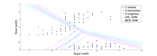
Figure 1: Experiment for separable dataset $\mathcal{D}_{\textrm{sep}}$

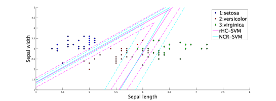
Figure 2: Experiment for non-separable dataset $\mathcal{D}_{\textrm{nsep}}$

To see the performance of the linear classifier as the solution of (17), we applied a Forward-Backward based Primal-Dual method [21, 22, 12] with $C=2^{10}$ to $\mathcal{D}_{\textrm{sep}}$ and $\mathcal{D}_{\textrm{nsep}}$.

To see the performance of the linear classifier as the solution of (26), we applied the proposed algorithmic solution in Theorem 1(c) to $\mathcal{D}_{\textrm{sep}}$ and $\mathcal{D}_{\textrm{nsep}}$.

For each linear classifier $\mathbf{p}=\mathbf{p}_{\textrm{NCR}}$ by (17) and $\mathbf{p}=\mathbf{p}_{\textrm{rHC}}$ by (26), the three decision boundaries $\Pi_{(\mathbf{p},\textrm{r,s})}^{0}(r<s)$ are drawn with solid lines in Fig. 2 for $\mathcal{D}_{\textrm{sep}}$ and in Fig. 2 for $\mathcal{D}_{\textrm{nsep}}$. The boundaries of $\Pi_{(\mathbf{p},\textrm{r,s})}^{[1,\infty)}(r\neq s)$ are drawn with dashed lines in Fig. 2 for $\mathcal{D}_{\textrm{sep}}$ and Fig. 2 for $\mathcal{D}_{\textrm{nsep}}$.

In Fig. 2, we observe that both linear classifiers achieve $\mathscr{E}_{\mathbf{p}_{\textrm{NCR}}}(\mathcal{D}_{\textrm{sep}})=\mathscr{E}_{\mathbf{p}_{\textrm{rHC}}}(\mathcal{D}_{\textrm{sep}})=0$ with smallest pairwise margins $\textrm{dist}\left(\Pi_{(\mathbf{p}_{\textrm{NCR}},2,3)}^{[1,\infty)},\Pi_{(\mathbf{p}_{\textrm{NCR}},2,3)}^{0}\right)=0.0467$ and
$\textrm{dist}\left(\Pi_{(\mathbf{p}_{\textrm{rHC}},2,3)}^{[1,\infty)},\Pi_{(\mathbf{p}_{\textrm{rHC}},2,3)}^{0}\right)=0.0681$ (Note: The solutions $\mathbf{p}_{\textrm{NCR}}$ of (17) with $C=2^{8}\ \textrm{and}\ 2^{9}$ result respectively in $\mathscr{E}_{\mathbf{p}_{\textrm{NCR}}}(\mathcal{D}_{\textrm{sep}})=3\ \textrm{and}\ 1$).

In Fig.2, we observe that both linear classifiers achieve $\mathscr{E}_{\mathbf{p}_{\textrm{NCR}}}(\mathcal{D}_{\textrm{nsep}})=16$ and $\mathscr{E}_{\mathbf{p}_{\textrm{rHC}}}(\mathcal{D}_{\textrm{nsep}})=7$ with smallest pairwise margins $\textrm{dist}\left(\Pi_{(\mathbf{p}_{\textrm{NCR}},1,3)}^{[1,\infty)},\Pi_{(\mathbf{p}_{\textrm{NCR}},1,3)}^{0}\right)=0.0503$ and
$\textrm{dist}\left(\Pi_{(\mathbf{p}_{\textrm{rHC}},1,3)}^{[1,\infty)},\Pi_{(\mathbf{p}_{\textrm{rHC}},1,3)}^{0}\right)=0.0702$.

These experiments demonstrate that the desired features in Remark 2 are achieved by the proposed algorithm in Theorem 1(c). We also observed the difficulty in parameter tuning for (17).

V CONCLUSION

We proposed the Robust Hierarchical Convex multiclass SVM and an iterative algorithm to realize this classifier. Numerical experiments demonstrate that the proposed multiclass classifier achieves larger smallest pairwise margin, even with smaller number of misclassified training samples, than a multiclass classifier [Crammer-Singer 2001] which has been known as a most natural multiclass extension of the soft-margin SVM.

References

• [1] C. Cortes and V. Vapnik, “Support-vector networks,” Machine Learning, vol. 20, pp. 273–297, 1995.
• [2] V. Vapnik, Estimation of Dependence Based on Empirical Data, Addendum I, Springer, 1982.
• [3] V. Vapnik, Statistical Learning Theory, John Wiley & Sons, 1998.
• [4] I. Yamada and M. Yamagishi, “Hierarchical convex optimization by the hybrid steepest descent method with proximal splitting operators - Enhancements of SVM and Lasso,” in Splitting Algorithm, Modern Operator Theory, and Applications, H. H. Bauschke, R. Burachik, and D. R. Luke, Eds. 77pp., Springer, 2019.
• [5] I. Yamada, “The hybrid steepest descent method for the variational inequality problem over the intersection of fixed point sets of nonexpansive mappings,” in Inherently Parallel Algorithms in Feasibility and Optimization and Their Applications, D. Butnariu, Y. Censor, and S. Reich, Eds., vol. 8, pp. 473–504. Elsevier, 2001.
• [6] V. Blanz, B. Schölkopf, H. Bülthoff, C. Burges, V. Vapnik, and T. Vetter, “Comparison of view-based object recognition algorithms using realistic 3D models,” in Proc. International Conference on Artificial Neural Networks. Springer, 1996, pp. 251–256.
• [7] U. H.-G. Kreßel, “Pairwise classification and support vector machines,” in Advances in Kernel Methods: Support Vector Learning, B. Schölkopf, C. Burges, and A. Smola, Eds. MIT Press, Cambridge, MA, 1999.
• [8] K. Crammer and Y. Singer, “On the algorithmic implementation of multiclass kernel-based vector machines,” Journal of Machine Learning Research, vol. 2, pp. 265–292, 2001.
• [9] J. Weston and C. Watkins, “Multi-class support vector machines,” Tech. Rep., Dept. Computer Science, Royal Holloway, University of London, 1998.
• [10] Y. Guermeur, “Combining discriminant models with new multi-class svms,” Pattern Analysis & Applications, vol. 5, pp. 168–179, 2002.
• [11] K. Tatsumi, K. Hayashida, R. Kawauchi, and T. Tanino, “Multiobjective multiclass support vector machines maximizing geometric margins,” Pacific Journal of Optimization, vol. 6, pp. 115–141, 2010.
• [12] G. Chierchia, N. Pustelnik, J.-C. Pesquet, and B. Pesquet-Popescu, “A proximal approach for sparse multiclass SVM,” arXiv preprint arXiv:1501.03669, 2015.
• [13] L. Wang and X. Shen, “On $l_{1}$-norm multiclass support vector machines: methodology and theory,” Journal of the American Statistical Association, vol. 102, pp. 583–594, 2007.
• [14] Y. Liu and X. Shen, “Multicategory $\psi$-learning,” Journal of the American Statistical Association, vol. 101, pp. 500–509, 2006.
• [15] H. H. Bauschke and P. L. Combettes, Convex Analysis and Monotone Operator Theory in Hilbert Spaces, Springer, 2nd edition, 2017.
• [16] N. Ogura and I. Yamada, “Non-strictly convex minimization over the bounded fixed point set of a nonexpansive mapping,” Numerical Functional Analysis and Optimization, vol. 24, pp. 129–135, 2003.
• [17] I. Yamada, M. Yukawa, and M. Yamagishi, “Minimizing the Moreau envelope of nonsmooth convex functions over the fixed point set of certain quasi-nonexpansive mappings,” in Fixed-Point Algorithms for Inverse Problems in Science and Engineering, H. H. Bauschke, R. Burachik, P. L. Combettes, V. Elser, D. R. Luke, and H. Wolkowicz, Eds., pp. 345–390. Springer, 2011.
• [18] J. Eckstein and D. P. Bertsekas, “On the Douglas-Rachford splitting method and the proximal point algorithm for maximal monotone operators,” Mathematical Programming, vol. 55, pp. 293–318, 1992.
• [19] H. H. Bauschke, Projection Algorithms and Monotone Operators, Ph.D. thesis, Simon Fraser University, 1996.
• [20] R. A. Fisher, “The use of multiple measurements in taxonomic problems,” Annals of Eugenics, vol. 7, pp. 179–188, 1936.
• [21] B. C. Vũ, “A splitting algorithm for dual monotone inclusions involving cocoercive operators,” Advances in Computational Mathematics, vol. 38, pp. 667–681, 2013.
• [22] L. Condat, “A primal-dual splitting method for convex optimization involving Lipschitzian, proximable and linear composite terms,” Journal of Optimization Theory and Applications, vol. 158, pp. 460–479, 2013.