Detection and Estimation of Local Signals

Abstract

We study the maximum score statistic to detect and estimate local signals in the form of change-points in the level, slope, or other property of a sequence of observations, and to segment the sequence when there appear to be multiple changes. We find that when observations are serially dependent, the change-points can lead to upwardly biased estimates of autocorrelations, resulting in a sometimes serious loss of power. Examples involving temperature variations, the level of atmospheric greenhouse gases, suicide rates, incidence of COVID-19, and excess deaths during the pandemic illustrate the general theory.

Keywords: segmentation, change-point, broken line, autoregression.

1 Introduction.

We consider a problem of detection, estimation, and segmentation of local nonlinear signals imbedded in a sequence of observations. As a model, we assume for $u=1,\ldots,T$

$$Y_{u}=\rho Y_{u-1}+\mu(X_{u})+\sum_{k}\xi_{k}f[(X_{u}-t_{k})/T]+\epsilon_{u},$$ (1)

where $t_{1}<t_{2}<\ldots<t_{M}$ define the locations and $f$ the “shape,” of the local signals. For asymptotic analysis given below, we assume that the $t_{k}$ are scaled, so $t_{k}/T=t_{0,k}$. Initially we assume the $X_{u}$ are fixed, but for some applications they are random. The $\epsilon_{u}$ are independent mean 0, normally distributed errors. For the moment we assume their variances are known and equal one, and discuss later how they should be estimated. The nuisance parameters $\mu(X_{u})$ depend on the variable $X_{u}$ and may be constant or a parameterized regression function. The purpose of introducing $\rho$ into our model is to decrease the risk of false positive errors if the observations are dependent, but it is not intended to be a good description of the true dependence. For our general theory we assume $\rho$ is an unknown constant, but for some applications we regard $\rho$ as a pre-whitening device and assign it an arbitrary numerical value, which may be altered in subsequent analysis if we appear to have made an inappropriate choice.

An important special case that we return to in examples below is $X_{u}=u$ and $\mu_{u}=\alpha+\beta[(u-(T+1)/2)/T]$, so with this notation the model becomes

$$Y_{u}=\rho Y_{u-1}+\mu_{u}+\sum_{k}\xi_{k}f[(u-t_{k})/T]+\epsilon_{u}.$$ (2)

It is sometimes convenient to simplify several basic calculations by considering an alternative continuous time model, for which (2) can be conveniently written

$$dY_{u}=-\gamma Y_{u}du+\mu_{u}du+\sum_{k}\xi_{k}f[(u-t_{k})/T]du+dW(u)$$ (3)

for $0\leq u\leq T$, where $dW$ defines white noise residuals.

A feature of all these models is statistical irregularity: $\xi_{k}$ and $t_{k}$ are confounded in the sense that if $\xi_{k}=0$, then $t_{k}$ is not defined. Specific choices of the function $f$ appear to be appropriate for a variety of applications, some of which are discussed below. The special case $f(x)=I\{x>0\}$ or $I\{0<x<\tau\}$ is a frequently discussed “change-point” model, which has been applied to a variety of problems, usually with $\rho$ assumed equal to 0. See, for example, Olshen et al. (2004), Robbins, Gallagher, and Lund (2016) and references given there. Fang, Li and Siegmund (2020) and Fryzlewicz (2014) address a version of the problem that involves the possibility of multiple change-points, and a major goal is segmentation of the observations to identify their number and locations, while controlling the probability of false positive detections. In this paper we extend the methods of Fang, Li and Siegmund (2020) to deal with more general signals and with observations that may have autoregressive dependence. See also Baranowski, Chen, and Fryzlewicz (2019).

A model with a long history, primarily for independent observations and at most one break-point, is a broken line regression model, where $f(x)=x^{+}$, so the model is given by

$$Y_{u}=\rho Y_{u-1}+\alpha+\beta[(u-(T+1)/2)/T]+\sum\xi_{k}[(u-t_{k})^{+}/T]+\epsilon_{u}.$$ (4)

An application to monitor kidney function after transplant has been discussed in a an elegant series of papers by A. F. M. Smith and others (e.g. Smith and Cook (1980)). Davies (1987) and Knowles and Siegmund (1989) give theoretical analyses for independent observations and at most one change-point. Toms and Lesperance (2003) provides an analysis and ecological applications. Several of the examples discussed below involve climatological time series, or day by day newly confirmed cases of COVID-19. Although alternative models are possible, a broken line model provides a simple conceptual framework that allows us to determine whether putative changes in direction of a regression function are real, and to suggest or confirm hypotheses of scientific interest. In particular, we can evaluate the evocative “hockey stick” suggested by the appearance of annual average temperatures of many countries in the 20th century.

In a variety of genomic applications $t$ denotes a genomic location, and different applications suggest functions $f$ having different characteristic shapes. For example, for detection of copy number variations (CNV) the indicator of an interval or a half line may be appropriate (e.g., Olshen et al. (2004), Fang, Li and Siegmund (2020)). For detection of differentially methylated genomic regions Jaffe, et al. (2012a) suggests a “bump” function. See simple examples in Appendix D of the Supplementary Material and elaborations of this model involving covariates in Jaffe, et al. (2012b). For ChIP-Seq analysis steeply decaying symmetric functions like $(1-|u|)^{+}$, $\exp(-|u|)$, or a normal probability density function are different possibilities (cf. Shin   et al. (2013), Schwartzman   et al. (2013)). In some applications it is often appropriate to add a scale parameter $\tau$, so at $u$ the signal located at $t$ is of the form $\xi f[(u-t)/(\tau T)]$ (cf. Siegmund and Worsley (1995)). The model of “paired change-points” of Olshen et al. (2004) can be described similarly, with $f(x)=I\{0<x\leq 1\}$.

In the special case that $\mu$ is a constant, $X_{u}=Y_{u-1}$, and $f(x)$ is the indicator that $x\leq 0,$ (1) is the simplest example of a threshold autoregression, as introduced by Tong and studied by Chan and Tong and others (e.g., Chan and Tong (1990) ) in numerous projects. In a still different context, $X_{u}$ may be a regressor, say a biomarker, and the local signal can be used to study whether a subset of individuals, defined by the value of that biomarker, differ from others in some respect, e.g., response to a treatment or disease susceptibility.

In some applications $X_{u}$ may be multidimensional or the noise distribution may not be normal, with the Poisson distribution representing a particularly interesting alternative.

In Section 2 we begin with some basic calculations and a discussion of testing for at most one change. We find two important features of our method. (i) The maximum likelihood estimator of $\rho$ under the hypothesis of no local signals can be badly biased when there are signals. (ii) The variance of the score statistic under the hypothesis of no signal, hence asymptotic evaluation of false positive error probabilities when $\rho$ is estimated by maximum likelihood does not depend on the value of $\rho$. We also develop confidence regions for $t$, which add appreciably to our understanding, and joint regions for $t$ and $\xi$.

A novel theoretical contribution are methods of segmentation, discussed in Section 3 and illustrated in 3.2. Two of the three methods suggested there are conceptually similar to methods proposed in Fang, Li and Siegmund (2020) for jumpchanges with independent observations, but their implementation is based on new probability approximations that involve random fields having smooth behavior in one coordinate and not smooth behavior in others. The third is a new procedure, which like circular binary segmentation (CBS,Olshen et al. (2004)) for the detection of jump changes, is designed to detect pairs of changes, but unlike CBS does not assume that the paired changes move in opposite directions.

If we assume as a consequence of segmentation that the $t_{k}$ in (2) are known without error, the model becomes a linear model. An important ingredient of our overall strategy is to use that linear model to evaluate the global success of our segmentation and to re-estimate the value of $\rho$, which is a lagged variable in the regression function. This provides the possibility of a re-segmentation if initially we used an inappropriate value. See Section 3.1 for examples.

Section 4 briefly considers the use of our methods for sequential detection of a change of slope in broken line regression, with examples from the COVID-19 pandemic.

Additional theoretical calculations and examples are contained in Supplementary Material.

Much although not all the related literature assumes independence, which seems adequate for many applications. We use a very simple model of dependence, defined in terms of the observed process, which makes that process first order Markov. Our goal here is not to build an approximately correct dependence structure, but to protect our methods for detecting changes in the mean value against an excess of false positives when the process exhibits dependence. At the cost of some computational complications we can also consider second or higher order Markov dependence.

There are alternative models of dependence, usually defined in terms of the unobserved residuals. See Robbins, Gallagher, and Lund (2016) for an interesting discussion using weak convergence arguments that involve rescaling the temporal and spatial coordinates. Explicit short term dependencies vanish in the limit, because points in the time scale that are separated by $o(m)$ are merged into a single point. This makes interpretation difficult if there appear to be nearby change-points in the original time scale.

Still other methods focus on estimation of the regression function (e.g., by a penalized likelihood), but do not provide statistical measures of the validity and variability in location of detected signals.

Our simple Markov model seems to provide a flexible technique to protect against an excess of false positive errors without a substantial loss of power.

2 Basic Calculations and the Case of at Most One Change.

To introduce our notation and provide some basic results, we begin with the model given by (2), with $M=1$ or 0, and we consider a test of the hypothesis $\xi=0$. The log likelihood is given by $\ell(\xi,t,\theta)$

$$=-\frac{1}{2}\sum_{u}\{Y_{u}-\rho Y_{u-1}-\alpha-\beta[(u-(T+1)/2)/T]-\xi f[(u-t)/T]\}^{2},$$

where $\theta=(\alpha,\beta,\rho)^{\prime}$, and we consider a test based on the maximum with respect to $t$ of the standardized score statistic

$$\ell_{\xi}(0,t,\hat{\theta})/\sigma(t),$$ (5)

where $\ell_{\xi}=d\ell/d\xi$, $\hat{\theta}$ is the maximum likelihood estimator of the nuisance parameters under the hypothesis $\xi=0$, and $\sigma^{2}(t)$ is the asymptotic variance of the numerator.

Our large sample theory begins with the standard expansion of the numerator in (5), given by

$$\ell_{\xi}(0,t,\hat{\theta})\approx\ell_{\xi}(0,t,\theta)-I_{\xi,\theta}I_{\theta,\theta}^{-1}\ell_{\theta},$$ (6)

where $I_{\cdot,\cdot}$ denotes elements of the Fisher information matrix and by the law of large numbers all quantities on the right hand side are evaluated at $\xi=0$ and true values of the other parameters. This expansion is valid in large samples up to terms that are $o(T)$ in probability. To emphasize the structure of this approximation we use the notation $\mathbb{E}_{0}$ to denote expectation under the hypothesis $\xi=0$ and write (6) in the form $V_{t}=\ell_{\xi}(t)-\Psi(t)^{\prime}A\ell_{\theta}$, where $\ell_{\xi}(t)=\ell_{\xi}(0,t,\theta)$, $\Psi(t)^{\prime}=\mathbb{E}_{0}[\ell_{\xi}(t)\ell_{\theta}^{\prime}]$ is not random although it depends on $t$; $\ell_{\theta}$ does not depend on $t$, and under the hypothesis $\xi=0$ it has mean value 0 and covariance matrix $A^{-1}=I_{\theta,\theta}$.

Remark. It may be shown that the decomposition given in (6) does not depend on the normality of the $\epsilon_{j}$, although we can no longer use the terminology of likelihood, efficient score, etc., and must rely on the central limit theorem to justify the asymptotic normality of probability calculations given below.

Calculations yield a number of simple propositions.

Proposition 1.

$$\Sigma(s,t)=\mathbb{E}_{0}(V_{s}V_{t})=\mathbb{E}_{0}[\ell_{\xi}(s)\ell_{\xi}(t)]-\Psi(s)^{\prime}A\Psi(t).$$ (7)

In particular the variance of $V_{t}$ is $\sigma^{2}(t)=\Sigma(t,t).$

Remarks. (i) Additional calculations show that $\Sigma(s,t)$ does not depend on unknown parameters. While this is expected and easily demonstrated for $\alpha$ and $\beta$, we found it tedious to demonstrate (cf. the online Supplementary Material) in the case of $\rho$. (ii) In the case the local signal contains a scale parameter, so it takes the form $\xi f[(u-t)/(\tau T)]$, the covariance is similar in its general formulation, but slightly more complicated to compute in examples.

Writing $\mathbb{E}_{t,\xi}$ to denote expectation under the alternative, where $t$ and $\xi$ can be vectors, we have

Proposition 2. $\mathbb{E}_{t,\xi}(V_{s})=\sum_{k}\Sigma(s,t_{k})\xi_{k}.$

Using Proposition 2, we can calculate numerically the expected sample path of $V_{s}$ or $Z_{s}=V_{s}/\sigma_{s}$ to see how we might go about detecting local signals. In the case that there is only one signal and, say, $\xi>0$, the expected path is typically maximized at $t$. Hence, if we assume there is at most one change at some unknown value $t_{0}$, we put $Z_{t}=[\ell_{\xi}(t)-\Psi(t)^{\prime}A\ell_{\theta}]/\sigma(t)$, and use the maximizing value of $|Z_{t}|$ as an estimator of $t_{0}$, provided $\max_{t}|Z_{t}|>b$ for a suitable threshold $b.$ (In Section 3 we discuss the segmentation of the values of $t$ in the case of multiple signals by considering local extrema of $|Z_{t}|$, judged against appropriate local backgrounds.)

For the case of at most one change, the false positive error probability is $\mathbb{P}_{0}\{\max_{t}|Z_{t}|\geq b\}$. To evaluate this probability, we distinguish essentially two cases, one where $f$ is continuous and the second where it is discontinuous. The case where $f$ is the indicator of a half line or an interval (of unspecified length) is discussed in Fang, Li and Siegmund (2020). Here we assume that $f$ is continuous and piecewise differentiable. An approximation based on Rice’s formula along the lines suggested by Hotelling (1939), Davies (1976) and others is given by

Proposition 3.

$$\mathbb{P}_{0}\{\max_{T_{0}\leq t\leq T_{1}}|Z_{t}|>b\}\leq 2\{(\varphi(b)/(2\pi)^{1/2})\int_{T_{0}}^{T_{1}}[\mathbb{E}_{0}(\dot{Z}_{t})^{2}]^{1/2}dt+1-\Phi(b)\},$$ (8)

where $\dot{Z}_{t}$ denotes the derivative of $Z$ at $t$. For the model where the local signal at $u$ has the form $\xi f[(u-t)/\tau T]$, and we maximize over both $t$ and a range of values of $\tau$, a first order approximation for large $b$ is

$$\mathbb{P}_{0}\{\max_{t,\tau}|Z_{t,\tau}|>b\}\sim 2\{b\varphi(b)/(2\pi)\}\int_{\tau_{0}}^{\tau_{1}}\int_{T_{0}}^{T_{1}}\rm{det}[\mathbb{E}_{0}(\dot{Z}\dot{Z}^{\prime})]^{1/2}dtd\tau,$$ (9)

where $\dot{Z}=\nabla Z_{t,\tau}$. This approximation can be improved by adding lower order terms involving edge effects and corrections for curvature. The most important is the boundary correction at the minimum value of $\tau$ equal to $(8\pi)^{-1/2}\varphi(b)\int_{T_{0}}^{T_{1}}[\mathbb{E}_{0}(\dot{Z})^{2}]^{1/2}dt$, where now $\dot{Z}=\frac{\partial Z}{\partial t}(t,\tau_{0})$. It is often convenient when $T$ is large to ignore edge effects. See Siegmund and Worsley (1995) or Adler and Taylor (2007) for more detailed approximations.

To evaluate (8) and (9), the following result is useful.

Proposition 4.

$$\mathbb{E}_{0}[(\dot{Z}\dot{Z}^{\prime})]=[\mathbb{E}_{0}(\dot{\ell}\dot{\ell}^{\prime})-\dot{\Psi}^{\prime}A\dot{\Psi}]/\sigma^{2}(t)-[\dot{\sigma}\dot{\sigma}^{\prime}]/\sigma^{2}.$$ (10)

Finally observe that by Propositions 1 and 2, we have the “matched filter” conditions, and consequently

Proposition 5. Given $t$ (or $t,\tau$), the variable $V_{t}$ (or $V_{t,\tau}$) is sufficient for $\xi$.

For the specific case of (4), it simplifies calculations somewhat to consider the continuous time version given in (3), which amounts to replacing certain sums by integrals, leading to

Proposition 6. $\sigma^{2}(t)\sim T\{(1-t_{0})^{3}/3-(1-t_{0})^{4}(1+t_{0}+t_{0}^{2})/3\}$, and $\mathbb{E}_{0}(\dot{V}_{t}^{2})\sim T\{(1-t_{0})-(1-t_{0})^{2}-3[t_{0}(1-t_{0})]^{2}\}.$

2.1 Confidence Regions

In this section we discuss confidence regions for the parameters $t$ or joint regions for $t$ and $\xi$. Calculation shows that the expected value of $V_{s}$ equals $\xi$ times the covariance of $V_{s}$ and $V_{t}$ (cf. Proposition 2). It follows from straightforward multivariate calculation that $Z_{t}=V_{t}/\sigma(t)$ is sufficient for $\xi$, so the conditional distribution of $Z_{s}$ given $Z_{t}$ is the same as it would be under the null hypothesis, $\xi=0$.

The case of jump changes was studied by Fang, Li and Siegmund (2020), so here we consider the case of continuous processes. For a similar approach based on a more complex probability evaluation see Knowles, Siegmund and Zhang (1991). Most of the examples given below involve broken line regression, where a changes occurs in the slope of (the expected value of) a process, but the process itself is continuous. An important distinction between changes in level and changes in slope is that the information about a change in level are usually found in a relatively small neighborhood of the change-point, whereas information about changes in slope can persist over long intervals. A consequence is that confidence regions for slope changes in broken line regression can be very large, even though the existence of a slope change seems obvious.

Although the method of Knowles, Siegmund and Zhang (1991) produces a conservative result under our assumptions, at least when $\rho=0,$ here we apply an asymptotic heuristic that is conceptually and technically simpler, and can be adapted (Section 3.1) to deal with multiple signals. The Kac-Slepian model process, for a mean 0 unit variance, twice mean-square differentiable, Gaussian process, say $U_{s}$, suggests a parabolic approximation for the process in a neighborhood of $s_{0}$. (This result is very similar to the local expansion of a quadratic mean differentiable log likelihood function, e.g., van der Vaart (1998)). By a tedious calculation of means and covariances, we see that

$$\mathbb{E}(U_{s}|U_{s_{0}},\dot{U}_{s_{0}})=U_{s_{0}}+(s-s_{0})\dot{U}_{s_{0}}-\frac{(s-s_{0})^{2}}{2}U_{s_{0}}\mathbb{E}_{0}[(\dot{U}_{s_{0}})^{2}]+o_{p}((s-s_{0})^{2})$$

and

$${\mathbb{V}}{\mathrm{a}r}(U_{s}|U_{s_{0}},\dot{U}_{s_{0}})=O((s-s_{0})^{4})$$

. These results and sufficiency (Proposition 5) suggest that in a neighborhood of a putative signal $t$, where $Z_{t}$ is large we consider the local approximation

$$Z_{t+\delta}\approx Z_{t}+\delta\dot{Z}_{t}-\frac{\delta^{2}}{2}Z_{t}\mathbb{E}_{0}[(\dot{Z}_{t}^{2}]).$$

Maximizing over $\delta$, we obtain

$$\max_{\delta}(Z_{t+\delta}^{2}-Z_{t}^{2})\approx\dot{Z}_{t}^{2}/\mathbb{E}_{0}[(\dot{Z}_{t})^{2}],$$ (11)

which is is approximately $\chi^{2}$ with one degree of freedom. By inverting this relation, we obtain as an approximate $1-\alpha$ confidence region the set of all $t$ that satisfy $Z_{t}^{2}\geq\max_{\delta}Z_{t+\delta}^{2}-\chi^{2}_{1-\alpha}$, where $\chi^{2}_{1-\alpha}$ is the $1-\alpha$ quantile of the $\chi^{2}$ distribution with one degree of freedom. This is in effect the same result one would obtain in large samples by inverting the log likelihood ratio statistic of a simple hypothesis if $Z^{2}$ were the log likelihood of a parameter satisfying standard regularity conditions. We conjecture that this approximation can be proved under additional regularity condtions, but here we use a small set of simulations to suggest it is reasonable.

A joint confidence region for $\xi$ and $t$ can also be obtained. To the condition that $Z_{t}^{2}$ must be within a given distance of $\max_{s}Z_{s}^{2}$, we also require that $|Z_{t}-\xi\sigma(t)|$ is sufficiently small. The pairs $\xi,t$ that satisfy $\max_{\delta}[Z_{t+\delta}^{2}-Z_{t}^{2}]+(Z_{t}-\xi\sigma(t))^{2}\leq c^{2}$ provide a joint confidence region having the confidence coefficient

$$\mathbb{P}_{t,\xi}\{\max_{\delta}[Z_{t+\delta}^{2}-Z_{t}^{2}]+(Z_{t}-\xi\sigma(t))^{2}\leq c^{2}\}$$ (12)

$$=\mathbb{E}_{t,\xi}[\mathbb{P}_{t,\xi}\{\max_{\delta}[Z_{t+\delta}^{2}-Z_{t}^{2}]\leq c^{2}-(Z_{t}-\xi\sigma(t))^{2}|Z_{t}\};|Z_{t}-\xi\sigma(t)|\leq c]$$ (13)

which equals the distribution of a $\chi^{2}$ random variable with two degrees of freedom, again as if standard regularity conditions had been satisfied.

In view of the heuristic elements of the preceding calculations, we give here the results of a small simulation that suggests our approach is reasonable. Consider a broken line regression model where observations have unit variance and the only nuisance parameters are unknown intercepts and slope. The sample size is 100. The slope is initally 0 and changes to $\xi$ at $t$.

Table 1: Confidence Sets for $t$. Number of repetitions is $N=1000$.

$t$	$\xi$	Nominal Conf.	Empirical Conf.	Expected Size
30	0.07	0.95	0.97	19
50	0.05	0.95	0.96	30
70	0.07	0.95	0.96	31
30	0.05	0.90	0.89	21
45	0.04	0.90	0.91	30
60	0.03	0.90	0.88	49
50	0.03	0.90	0.89	42

2.2 Numerical Examples

Example 1. Extreme Precipitation in the United States. Extreme precipitation in the United States is reported by the National Oceanographic and Atmospheric Administration (NOAA) at https://www.ncdc.noaa.gov/temp-and-precip/uspa/wet-dry/0.

This web site gives the area of the country where monthly rainfall exceeeded the 90th percentile of normal for the 125 years beginning in 1895.

Our test for at most one changes suggests a slope increase at 707 months, in 1954, with a p-value of 0.002. The value of $\rho$ is estimated to be 0.08. The test applied to extremely low preciptation (area of the country below the 10th percentile) is consistent with the hypothesis of no change in slope.

Example 2. Central England Annual Average Temperature. The average temperature in central England from 1659 (Manley (1974)) until 2019 is reported https://www.metoffice.gov.uk/hadobs/hadcet/cetml1659on.dat.

The maximum $Z$ value is about 4.60, with $\rho$ estimated to be 0.16, and occurs in 1969. The appropriate (two-sided) p-value is about $6\times 10^{-5}$. See Figure 1, where it appears that there might also be earlier change-points. Although the mercury thermometer was relatively young in 1659, those early years are interesting since they appear to involve the “little ice age.” We return to these data below for our discussion of segmentation. Meanwhile it may be interesting to note that an approximate 95% confidence region based on the detected change in 1969 is (1895,1990), which reflects the local shape of the plot in Figure 1 and suggests the possibility that an increase in temperature may have actually begun during the late 19th century.

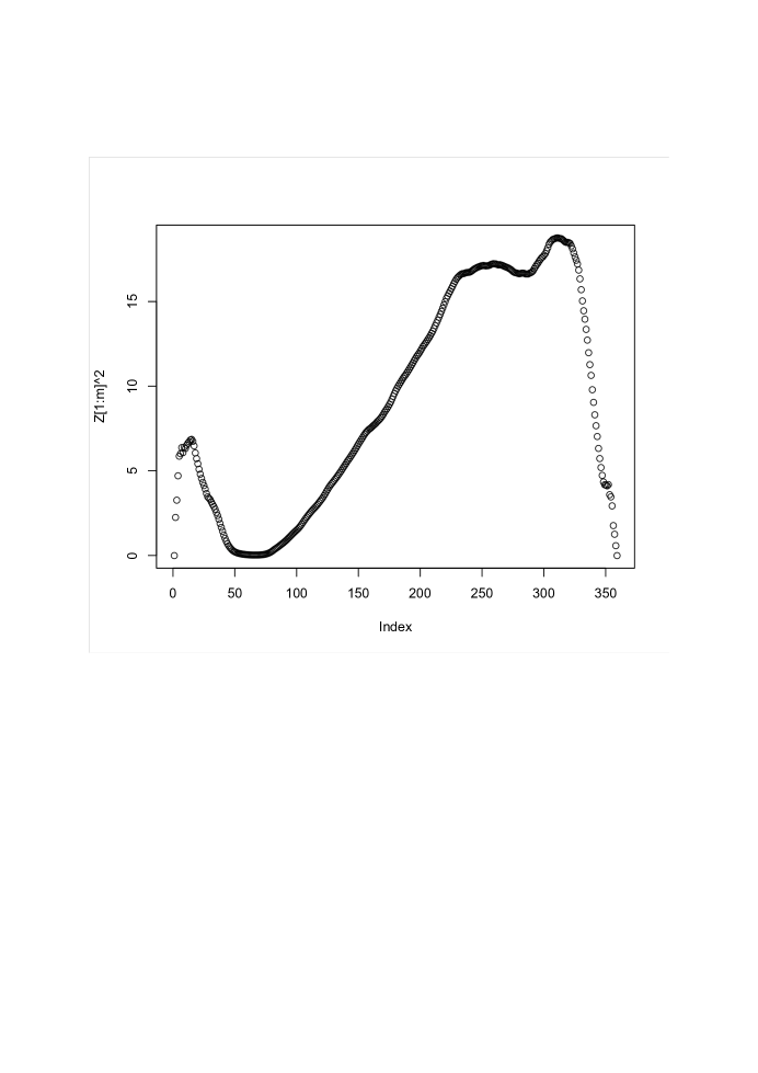
Figure 1: Plot of $Z_{t}^{2}$ for central england temperature data, 1659-2017.

Although we did not include a confidence region for Example 1, in that case also, the plot of $Z_{t}^{2}$ exhibits two local maxima and a confidence region substantially longer to the left than to the right of the maximizing value.

2.3 Estimation of $\sigma^{2}$ and $\rho$: Simulations.

Although we have assumed the variance known in our theoretical calculations, in our numerical studies we have estimated it by the residual mean square under the null hypothesis. Other possibilities when the data are independent, which may be less biased, are sums of squares of first or second order differences: $\sum_{u}(Y_{u+1}-Y_{u})^{2}/2m$ or $\sum_{u}(Y_{u+1}-2Y_{u}+Y_{u-1})^{2}/6m$., First order differences remove most of the effect of changing mean values, and second order differences also mitigate the effect of slope changes.

Regarding correlation of the observations, a useful model is one that helps to control false positive errors with minimal loss of power, but otherwise estimating $\rho$ efficiently is unimportant. Using a value of $\rho$ that is much too small can lead to an increase in false positives. But in the presence of change-points, the maximum likelihood estimator of $\rho$ under the null hypothesis that $\xi=0$ can be upwardly biased, leading to a loss of power.

In Table 2 we consider the control of false positive errors when true and assumed first order autocorrelations differ. The column labeled $\hat{\rho}$ contains assumed values, not estimates.

Table 2: Simulated False Positive Errors: $m=100$, 0.05 threshold is $b=2.84$. Number of repetitions is $N=900$.

$\rho$	$\hat{\rho}$	$\mathbb{P}\{\max_{s}|Z_{s}|\geq b\}$
0	0	0.033
0.3	0	0.12
0.3	0.1	0.076
0.3	0.2	0.050
0.5	0.3	0.043
0.6	0.3	0.051
0.7	0.3	0.059
0.8	0.3	0.081
0.9	0.35	0.049
0.8	0.4	0.023
0.9	0.4	0.036

The simulated example in Table 3 illustrates the problem of estimating $\rho$ and the effect on the power to detect a change.

Table 3: Simulated examples: $m=150$, 0.05 threshold is $b=2.83$. Locations of break-points and changes in the slope occurring at the break-points are as indicated. Rows where $\hat{\rho}$ has been set equal to $\rho$ are included to illustrate the loss of signal that occurs because of bias in estimation of $\rho$.

$t$	$\xi$	$\rho$	$\hat{\rho}$	$\hat{\sigma}$	$\max_{s}|Z_{s}|$
—	0.00	0.50	0.48	0.98	1.60
—	0.00	0.60	0.56	0.98	1.05
100	0.05	0.0	0.30	1.04	4.04
100	0.05	0.0	0.00	1.09	5.51
100	0.05	0.4	0.60	1.19	3.86
100	0.05	0.6	0.75	1.00	3.34
100	0.05	0.6	0.60	1.02	5.06
50	0.04	0.5	0.54	0.97	3.37
50	0.04	0.5	0.50	0.97	3.66
50	-0.033	0.6	0.76	1.15	2.74
50	-0.033	0.6	0.60	1.15	4.34

For the data in the third and fourth rows of Table 2, According to Proposition 2, the expectation of $Z_{t}$ is 5.55, so the simulated value when it is known that $\rho=0$ and $\sigma$ is estimated to be 1.09 is very accurate. In that case, if we use second order differences to estimate $\sigma^{2}$, the estimated value of $\sigma$ is only 0.89 and the maximum $Z$ value is 6.77. In both rows 3 and 4, the maximizing value of $t$ is 94.

It is apparent from Table 2 and other examples not shown that the existence of a change-point causes the estimator of $\rho$ to be upwardly biased and results in a loss of power compared to using the true value. This is usually worse if there are multiple change-points. If a plot of the data indicates long stretches without change-points, one might use an estimator of $\rho$ from that segment. For the data in the next to last row of Table 1, an estimate of $\rho$ based on the observations 65-150 yields the value 0.61, which in turn leads to a maximum $Z$-value of 4.31. Although the theory developed here does not justify this approach, numerous simulations suggest that it works reasonably well. (See also the discussion of the Atlantic to use an arbitrarily chosen value of $\rho$ to pre-whiten the observations and repeat the analysis if that value appears to be poorly chosen.

A second consideration in estimation of $\rho$ is robustness of our procedure against more complex forms of dependence. Without exploring this question in detail, consider again the next to last row of Table 1, but with a second order autoregressive coefficient of - 0.2 and $\xi=-0.06$. A simulation of this case gives an estimator of $\rho$ equal to 0.6 based on all the data, with a maximuom $Z$-value of 3.32, and an estimator equal to 0.42 based on the second half of the data, with a maximum $Z$-value of 4.85. Other simulations, not given here, suggest that at least for higher order autoregressive dependence, the first order model we have suggested provides reasonable protection against an inflated false positive error rate.

3 Segmentation.

We now turn to the problem of segmentation when there may be several change-points. It is helpful conceptually to think of two different cases. In the first the signals exhibit no particular pattern. In the second two or more changes are expected to produce a definite signature. For the problem of jump changes in levels of the process, paired changes frequently take the form of an abrupt departure from followed by a return to a baseline level. Here we concentrate on the case of signals having no apparent pattern.

The simplest method is binary segmentation: first we test for at most one change, then iteratively partition the data at a putative change-point to test for additional changes to the left or the right of the detected change-point. A definite disadvantages of this method is that positive and negative changes in the same sequence of observations may cancel and lead to a loss of power to detect any change. In addition, for slope changes the score statistic has substantial local correlation, so it can occur that a second change is detected very close to the first unless the interval searched is restricted so that its end-points are some arbitrary distance away from already detected change-points.

Next we consider versions of the two methods suggested in Fang, Li and Siegmund (2020) for detection of jump changes. First we consider a pseudo-sequential procedure, called Seq below, where it is convenient to write $Z(t,T)$ to denote the statistic $Z(t)$ when the interval of observation is $[0,T]$. We also use a minimum sample size $m_{0}$ and a minimum lag $n_{0}$, both of which we often set equal to 5. Let $t_{0}=m_{0}$ and let $T$ be the smallest integer exceeding $t_{0}+n_{0}$ such that for some $t_{0}<t<T-n_{0}$, the value of $Z(t,T)$ exceeds a threshold $b$ to be determined by a constraint on the probability of false positive error. The first change-point is taken to be $t_{1}$: equal to $\arg\max|Z_{t}|$, or the smallest or largest value of $t$ for that smallest $T$. (In numerical experiments we have been unable to find a consistent preference.) The process is then iterated starting from $t_{1}$. The nuisance parameter $\rho$ is assumed to be known. In practice it is estimated from the data or more often from a subset of the data to mitigate the effect of the bias discussed above. The other nuisance parameters, are estimated from the current, evolving interval of observations, so that the nuisance parameters associated with one change-point do not confound detection of another. It would also be possible to estimate $\rho$ from the currently studied subset of the data, but this estimator appears to be unstable.

To control the global false positive error rate, we want an approximation for

$$Q=\mathbb{P}\{\max_{m_{0}\leq t<T-n_{0},T\leq m}|Z(t,T)|\geq b\},$$

where $m$ is the number of observations and $m_{0},n_{0}$ represent minimal sample sizes, both of which we frequently take to be 5. To emphasize that $T$ is a variable quantity, we also write $\sigma^{2}(t,T),$ $\Psi(t,T)$, etc.

Theorem 1. Let $\beta(t,T)=\{\mathbb{E}[V\partial V/\partial T)-\frac{1}{2}\partial\sigma^{2}(t,T)/\partial T\}/\sigma^{2}(t,T)$ and $\lambda_{t}=\mathbb{E}[(\dot{Z}_{t,T})^{2}].$ Assume that $\Delta$ and $\delta$ are positive constants converging to 0. Assume $b\rightarrow\infty$ and $b^{2}\Delta$ converges to a positive constant, while $b\delta\rightarrow 0.$ Then

$$Q\sim(2/\pi)^{1/2}b^{2}\varphi(b)\int_{m_{0}}^{m}\int_{m_{0}<t\leq T-n_{0}}\{\lambda_{t}^{1/2}\beta(t,T)\nu[b(2\beta(t,T)\Delta)^{1/2}]\}dtdT.$$ (14)

For a proof we also assume that $m$ is not too large relative to $b$, e.g., that $m=o(\exp(b^{2}/8))$, which ensures that asymptotically $Q$ is a small tail probability. (See Remark (iii) below.)

For $t=i\delta$ and $T=k\Delta$, we write the probability of interest as a sum over $T$ of the sum over $t\leq T-n_{0}$ of the integral over $x>0$ of the product of three factors: (i) $\mathbb{P}\{Z(t,T)\in b+dx/b\}\sim\varphi(b)\exp(-x)dx/b;$ (ii) $\mathbb{P}\{\max_{j\geq 1}b[Z(t,T-j\Delta)-Z(t,T)]<-x|Z(t,T)=b+x/b\}.$ and (iii) the conditional probability that $[Z(t\pm\delta,T)-Z(t,T)]<0$. The argument of (for example) Theorem 2.1 of Fang, Li and Siegmund (2020) shows that in the limit the conditional probability (ii) converges to a probability of the form $\mathbb{P}\{\max_{j\geq 1}S_{j}<-x\}$, where $S_{j}$ is a Gaussian random walk with mean equal in the limit to $\beta b^{2}\Delta$ and variance $2\beta b^{2}\Delta$. The integral over $(0,\infty)$ of $\exp(-x)$ times this probability equals $\beta b^{2}\Delta\nu[b(2\beta\Delta)^{1/2}]$, where $\nu$ is the function defined in Siegmund (1985) and easily approximated numerically. By the Kac-Slepian approximation, for small $s$, $Z(t+s,T)-Z(t,T)=s\dot{Z}(t,T)-s^{2}\lambda Z(t,T)/2+o_{p}(s^{2})$, where $\dot{Z}$ is normal with mean 0 and variance $\lambda$. Hence the conditional probability in (iii) equals $\Phi(\lambda^{1/2}b\delta/2)]-\Phi(-\lambda^{1/2}b\delta/2)$. Since $b\delta\rightarrow 0,$ this last expression is asymptotic to $\lambda^{1/2}b\delta/(2\pi)^{1/2}.$ Putting these pieces together and replacing the sums by Riemann integrals yields (14).

Remarks and Examples. (i) In (14), we treated the process $Z(t,T)$ as continuous in $t$ and have used $\delta$ and $\Delta$ as a differentials to replace sums by integrals.. In applications we always take $\Delta=1,$ so one could leave the integral over $T$ in the form of a sum. Numerically this makes essentially no difference. We could also take $\Delta$ to 0 faster than $1/b^{2}$, which would effectively treat the process in $T$ as a continuous, but not differentible, process. This leads to a very conservative approximation if the process is approximately Gaussian, but presumably more robust to departures from normality. (ii) For a numerical example, suppose $m=365$, $b=4.0(4.41)$, $m_{0}=n_{0}=5.$ Then (14) gives the approximation 0.05 (0.01). When $T$ is allowed to vary continuously, the threshold corresponding to 0.05 (0.01) is 4.43(4.80.) A small simulation with $m_{0}=n_{0}=5$ and a sample size of 10000 to test the accuracy of the first set of thresholds gave the values 0.0493 and 0.0111.

(ii) It is possible to make the preceding argument rigorous, but the many details that one can see in related arguments suggest that a complete proof would be onerous and not add any new insights (cf. Siegmund and Yakir (2000), Fang, Li and Siegmund (2020)).

(iii) The condition that $m$ not be too large compared to $b$ guarantees that there is asymptotically at most one excursion above a high threshold $b$, so the right hand side (RHS) of (14) converges to 0, and hence our approximation lies in the domain of small tail probabilities. For much larger $m$, there can be several excursions above $b$, so RHS(14) may be bounded away from 0, and one expects in that case that a suitable approximation has the form $Q-[1-\exp[-RHS(\ref{segmentprob})]\rightarrow 0.$ See Siegmund and Yakir (2000) for the global arguments for a similar example.

(iv) When the process $Z(t,T)$ exceeds a suitable threhold, there is typically a cluster of values of $T$ and $t$ where $|Z(t,T)|$ exceeds that threshold. In practice we might for the smallest such $T$ choose as an estimate of the position of a slope change the smallest $t$, the value that maximizes $|Z(t,T)|$, or perhaps some other value. One hopes that experience eventually suggests an optimal choice of $t$, but that does not seem to be the case. Examples where there is only a small number of values of $T$ and $t$ with the values of $t$ only slightly smaller than $T$ may indicate the presence of outliers and suggests that we skip to a larger value of $T$. Once a value of $t$ is selected, we then iterate the process starting from that $t$, and the background linear regression is estimated using the data beginning with that $t$.

(v) We have used the term “pseudo-sequential” since most applications discussed in this paper involve a fixed amount of data. However, we estimate $\alpha$, $\beta$ and $\sigma^{2}$ using the data since the last change detected, so the method can also be applied sequentially. See Section 4 for an application to detecting upswings in COVID-19..

A second method of segmentation, called MS below (for Maximum Score Statistic), uses (in obvious notation)

$$\max_{m_{0}\leq T_{0}<t<T_{1}<m}Z_{T_{0},t,T_{1}}.$$

An asymptotic approximation to the null probability that this expression exceeds $b$ can be computed as a corollary of the argument behind Theorem 1, and we obtain the approximating expression

$$(\frac{2}{\pi})^{1/2}b^{4}\varphi(b)\times$$

$$\sum_{m_{0}\leq T_{0}<T_{1}\leq m}\int_{T_{0}<t<T_{1}}(\lambda_{t})^{1/2}\beta_{0}(t,T_{0})\beta(t,T_{1})\nu\{b[2\beta_{0}(t,T_{0})]^{1/2}\}\nu\{b[2\beta(t,T_{1})]^{1/2}\}dt,$$ (15)

where $\beta_{0}(t,T_{0})$ is defined similarly to $\beta(t,T)$. The evaluation of (15) can be simplified by a summation by parts and the observation that the various functions of three variables, $(T_{0},t,T_{1})$, occurring in (15) are in fact functions of two variables: $(t-T_{0},T_{1}-T_{0})$.

This method determines a list of putative local signals together with generally overlapping backgrounds. We consider different algorithms for selecting a set of local signals and backgrounds from this list, with a preference for the additional constraint that no background overlap two local signals. In Fang, Li and Siegmund (2020) examples of particular interest were the shortest background, (cf. also Baranowski, Chen, and Fryzlewicz (2019)), and the largest $Z$ value. Since we have paid in advance for false positive errors, we can also consider other methods for searching the list, e.g., subjective consistency with a plot of the data. We also find it convenient computationally to follow the suggestion of Fryzlewicz (2014) by searching a random subset of intervals, which seems to work very well. When it appears that the number of changes is small, as in the examples considered in this paper, one might also use a combination of methods, e.g., searching a small random subset of intervals at a low threshold to generate candidates, then sorting those by hand with tests to detect at least one change at the appropriate higher threshold.

The methods Seq and MS “bottom up” methods in the sense that they attempt to identify one local signal at a time against a background appropriate for that signal–an advantage if there is heterozygosity.

A popular “top down” method to detect abrupt level changes scans all the data looking for a pair of change-points (e.g., Olshen et al. (2004)). In some cases, especially if there is only one change to be detected, the method will “detect” two changes, as required, but it will put one of them near an end of the data sequence, where it can be recognized and ignored. After an initial discovery of one or two change-points, the sequence is broken into two or three parts by those change-points, and the process is iterated as long as new change-points are identified. Consider the statistic $\max_{s<t-h}R(s,t)$, where

$$R^{2}(s,t)=(Z_{s},Z_{t})\tilde{\Sigma}_{s,t}^{-1}(Z_{s},Z_{t})^{\prime},$$ (16)

$\tilde{\Sigma}$ is the covariance matrix of $(Z_{s},Z_{t})^{\prime}$, and $h$ is a parameter that represents a minimum distance between changes that we find interesting (usually taken to be 5 or 10 in the examples below). An appropriate threshold may be determined from an approximation similar to (9) although the details are substantially more complicated, since $R(s,t)$ is related to, but is not a Gaussian process.

Let $\rho=\rho(s,t)$ denote the correlation of $Z_{s}$ and $Z_{t}$ and put $U(\theta,s,t)=\cos(\theta)Z_{s}+\sin(\theta)(Z_{t}-\rho Z_{s})/(1-\rho^{2})^{1/2}$. Then $U$ is a Gaussian process and $R(s,t)=\max_{\theta}[U(\theta,s,t)].$ Now a formula similar to (9) is applicable. Computation of the final result is complicated by the fact that the integral is three dimensional and involves the determinant of the $3\times 3$ covariance matrix of $\dot{U}=(U_{\theta},U_{s},U_{t})^{\prime}$, where subscripts denote partial derivatives. The result is

Theorem 2. As $b\rightarrow\infty$,

$$\mathbb{P}\{\max_{s<t-h}R(s,t)>b\}\sim[b^{2}\varphi(b)/(2\pi)^{3/2}]\int_{0<\theta<2\pi,s<t-h}{\rm det}[\mathbb{E}(\dot{U}\dot{U}^{\prime})]^{1/2}d\theta dsdt.$$ (17)

3.1 Confidence Regions Revisited.

We can also use (16) to find confidence regions for two (or more) change-points $t_{1}<t_{2}$. First note that with $t=(t_{1},t_{2})$, and $\xi=(\xi_{1},\xi_{2})$, a straightforward calculation extending the result given in Proposition 2 shows that $\mathbb{E}_{t,\xi}(V_{s})=\sum_{i}[\xi_{i}\sigma(t_{i})\Sigma(s,t_{i})]$, where $\Sigma(s,v)={\mathbb{C}}{\mathrm{o}v}(V_{s},V_{v}).$ This produces by a second calculation the conclusion that the log likelihood of $V_{s},s=1,\cdots,T$ equals $\sum_{i}\xi_{i}\sigma(t_{i})V_{t_{i}}-.5\sum_{i,j}\xi_{i}\xi_{j}\sigma(t_{i})\sigma(t_{j})\Sigma(t_{i},t_{j})$. Hence the log likelihood ratio statistic, given $t$, for testing that $\xi$ is the 0 vector equals

$$(V_{t_{1}},V_{t_{2}})\Sigma(t_{1},t_{2})^{-1}(V_{t_{1}},V_{t_{2}})^{\prime}=||\tilde{Z}_{t_{1},t_{2}}||^{2},$$ (18)

where $\tilde{Z}_{t_{1},t_{2}}=\Sigma(t_{1},t_{2})^{-1/2}(V_{t_{1}},V_{t_{2}})^{\prime}$ has a standard bivariate normal distribution when $\xi=0$, and $||\cdot||$ denotes the Euclidean norm. It follows from sufficiency and the Kac-Slepian argument used above that

$$\max_{\delta_{1},\delta_{2}}[||\tilde{Z}_{t_{1}+\delta_{1},t_{2}+\delta_{2}}||^{2}-||\tilde{Z}_{t_{1},t_{2}}||^{2}]$$

has a $\chi^{2}$ distribution with two degrees of freedom and can be used as above to obtain a joint confidence region for $(t_{1},t_{2})$.

A joint confidence region for $t,\xi$ follows by an argment similar to that given above.

3.2 Applications.

In this section we consider a number of data sets, where broken line regression may be an appropriate model. Although it may not fit the data globally as well as other possibilities, it suggests questions regarding the times of sharp changes of direction and reltively small changes in long term trends. Since all these examples involve observational time series, an assumption of independence seems inappropriate, although in several cases the estimated value of $\rho$ is small enough to be assumed equal to zero.

As a step in our evaluation of the segmentation methods of Section 3, we assume that the detected changes are in fact correct,so our model becomes a standard linear model, with $\rho$ the coefficient of a one-step lagged regressor. Estimation of the regression parameters of that model with the change-points assumed known provides an idea of the size and importance of different detected changes, the adequacy of the model as judged by the value of $R^{2}$ and $\hat{\rho}$, and the reasonableness of our choice for the value of $\rho$ in our initial segmentation. In cases where the number of changes may be in doubt, e.g., when the method MS detects fewer changes, probably because of its stricter significance standard, we also compute a BIC score for the model with the larger number of slope changes compared to the model with fewer slope changes. Although the broken line model is an irregular statistical model, according to calculations in the unpublished Ph. D. thesis of Yi Liu, the customary assessment of a penalty by counting parameters (multplied by the log sample size) is the same as for a regular model.

In the figures that follow, we have plotted the data superimposed on the results of a multiple regression analysis. For ease of viewing the autocorrelation is not incorporated into the plot, although it is included in the evaluation of $R^{2}$.

Example 3: World Average Land and Ocean Temperature Anomalies: 1850-2020

Temperature anomaly time series are calculated by the Hadley Center in Great Britain, NOAA and the Goddard Institute for Space Sciences (GISS) in the United States, and by Berkeleyearth. Presumably approximately the same data from the same instruments are available to all groups, which they then process by different methods. The main obvious difference is the beginning date for the different time series: 1850 for the Hadley Center, 1880 for NOAA and GISS, and varying times for different countries, some as early as about 1750 for Berkeleyearth.

The data we consider in this example are the Hadley Center time series for land and ocean temperature anomalies, which begins in 1850 and contains 171 observations. Using MS with $\rho=0.2$, we detected three slope changes, an increase in approximately 1910, a decrease in 1942, and a final increase in 1977. The output of a linear analysis using those three changes is displayed in Figure 2. Since the data appear heteroscedastic, with more variability at the beginning of the series, in our linear model we used a weighted analysis, with weights derived from the uncertainty measures given for the data. The value of $R^{2}$ is estimated to be 0.89, and the value of $\rho$ is estimated to be about 0.3. With this value of $\rho$, both Seq and (16) suggest essentially the same three changes. MS and Seq, which detect changes against a local background, give roughly the same estimate of $\sigma^{2}$, which suggests that heterozygosity is not a serious problem for these data.

We discuss some related series and the problem of heterozygosity in the Online Supplement.

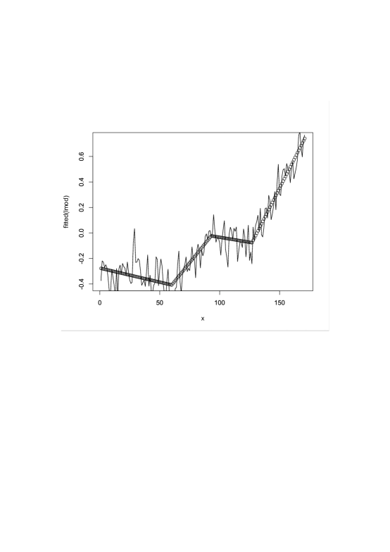
Figure 2: Linear Analysis of Annual World Land and Ocean Anomalies: 1850-2020.

Example 4. Excess Deaths in the United States. We consider next the number of excess deaths in the U.S beginning with the first week of January 2020. To avoid the problem of late reporting of deaths, we used 86 weeks, although 93 were available when this manuscript was written. An interesting feature of excess deaths is that on the one hand they account both for deaths from COVID-19 and deaths that occurred because appropriate medical care was unavailable due to the pandemic, and on the other they do NOT count deaths from influenza that did not materialize because responses to the pandemic.

For these data (16) with $\rho=0.3$ detected eight slope changes. Seq missed the first slope change, but otherwise agreed to within one week on the other detections. Results displayed in Figure 3 show a linear analysis with the changes suggested by (16) with some visually suggested adjustments to agree with Seq. For this linear analysis $R^{2}\approx 0.97$ and $\rho\approx 0.19$.

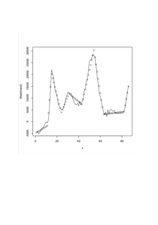
Figure 3: Linear Analysis of Excess Deaths in U.S. for 86 weeks from 01/01/2020.

Example 2 revisited: Central England Average Annual Temperature. A challenging case for segmentation is the central England temperature data for 361 years beginning in 1659. A plot of the data suggests possible changes very early in the series with a much larger change 2-3 hundred years later. The first 80-100 years may be less reliable, due to the relatively primitive thermometers available at that time, but the early data are nonetheless interesting in view of the “little ice age,” which overlapped these years. As reported above, a test of at least one change produces a significant increase in slope in 1970 with an estimated autocorrelation of 0.159, and a confidence interval going back about a hundred years, reflecting the increase in the plot of $Z_{t}^{2}$ in Figure 2 that begins in the late 19th century. If we use Seq with the threshold 4.4 and the autocorrelation 0.1, we obtain a broken line that decreases steeply for the first 33 years, then increases for about 16, bringing it back more or less to where it started. It then has a slightly negative slope until about 1890, when it begins to increase. No further increase in the 20th century is detected, which is perhaps surprising given our results when testing for at most one change and an accelerated rate of increase starting about 1970 for many other temperature series. For MS with a threshold of 4.81 and the same value for $\rho$, we find evidence for a change in 1890 or in 1983, without a compelling reason to choose one of the other.. Figure 3 suggests that either (or both) could be correct. A linear analysis indicates that the model with early changes in 1692 and 1708, then a later change in either 1890 or 1983 (not both) leads to an $R^{2}$ of approxmately 0.31 and a value of $\rho\approx 0.1$. The statistic (20) to detect two changes at a time detects changes in 1693, 1708, and 1978. BIC has a prefernce for three slope changes over four and a very small preference for the change in 1890 over the change in 1983.

Example 5: Age specific suicide rates in the United States. A small sample size example is suicide rates in the US from 1990 through 2017, which can be found on the web site ourworldindata.org. Autocorrelation appears to be very small, so we assume it is 0. All methods detect a substantial slope increase about 2000. For MS this is the only change detected, and it produces an $R^{2}$ of 0.91. Seq detects in addition, a second increase about 2014. The statistic (16) detects three changes, a decrease in slope about 1995 before a large increase in 1999, and a third increase in 2014. A linear analysis with all three changes yields an $R^{2}$ of 0.97.

4 Sequential Detection.

In this section we consider using Seq for online detection of slope changes, which for independent normally distributed observations has been studied using different metholds by Krieger, Pollak and Yakir (2003). We estimate the nuisance parameters locally, so that when we have observed $Y_{S},\ldots,Y_{T}$, we use only those values to estimate the nuisance parameters $\alpha$, $\beta$, and $\sigma^{2}$. Since estimates of $\rho$ are unstable when sample sizes are small, here we set $\rho=0$ and consider the possibility of reanalyzing the data with a different value if autocorrelation appears to play an important role.

We begin by considering the data for patient B in Smith and Cook (1980), one of a beautiful series of papers by Smith and co-authors concerned with monitoring renal transplants for rejection. The data are given graphically in the paper, and by eye we extracted the 10 daily values 35,45,49,64,75,71,69,60,31,21. Using Seq with the 0.05 threshold $b=2.56$, we find after 8 observations that a change has been detected and estimate the change to occur with the 6th observation. A linear analysis with this change-point indicates that the autocorrelation of 0 is reasonable and $R^{2}\approx 0.92$.

Several features of the COVID-19 pandemic provide interesting examples where broken line regression might be useful. First we consider the possibility of sequential detection of a a slope increase in daily incidence in the initial phase of the pandemic and allow a probability of 0.05 (or 0.01) of incorrectly detecting a slope increase within one year. By (14) with $m_{0}=m-m_{1}=5$, this produces a (one-sided) threshold of $b\approx 3.81(4.24)$.

Data are from ourworldindata.org.

As a first example we consider South Korea, which experienced its first case on 20 January, 2020. On 21 February, both the 0.05 and 0.01 thresholds were crossed and the change attributed to 6 days earlier.

A second example is Italy, which experienced its first cases on 31 January. Using either the 0.05 or the 0.01 criterion, we detect a slope increase on 26 February and estimate the change to have occurred about 5 days earlier. A “lockdown” of the entire country appears to have occurred on 11 March.

Remarks. A potential difficulty with the sequential application of our model in the initial phase of an epidemic is that detection of an increase in slope may occur while the sample size is still small, so using a normal approximation may be anti-conservative. An alternative leading heavier tail probabilities would be to assume a Poisson model with a constant mean value that may at some point start to increase linearly. Different possibilities for development are (i) to extend our theoretical calculations, (ii) simulate a threshold to check and perhaps adjust results based on an assumption of normality, or (iii) do a linear analysis of a log linear Poisson model to confirm the results. For the two examples given above, informal analysis confirms the results given. In other examples, detection was delayed by one or two days.

The sequential method may also be helpful in detecting second and third waves of infections following a relatively quiescent interval. We consider Santa Clara County, California, which like localities in the United States experienced a very large number of cases in early 2021, followed by a sharp decline in daily incidence during May. We use data from data.scc.org.gov. On 1 June, after a month when the daily incidence had been decreasing to fewer than 100 cases a day in a population of about two million, we started Seq with $\rho=0.5$, which is approximately the value given by a complete segmentation of 600 observations. The result with a (two-sided) 0.05 threshold was detection of a slope increase in the middle of July that was estimated to have begun during the last week of June. Using the 0.01 threshold delayed detection by 6 days.

5 Discussion.

We have studied score statistics to detect local signals in the form of changes of level, slope, or (in the online Supplement) the autoregressive coefficient. To segment the observations, we consider two “bottom up” methods patterned after the methods of multiple change-point segmentation in Fang, Li and Siegmund (2020) and one new “top down” method, defined in (16). The three methods have different strengths and weaknesses. Although both bottom up methods can be applied algorithmically, it appears to us that satisfactory segmentations often require some judgment regarding the appropriate number of changes and their locations. The method Seq can be applied sequentially if it is important to detect a change in slope quickly after its occurrence.

Asymptotic approximations for false positive error probabilities for the three methods appear to be new. For the bottom up methods the approximations involve random fields that are differentiable in one coordinate, but not differentiable in others. Both the statistic that tests for at most one change and (16) can be used to obtain confidence regions.

Estimation of the nuisance parameters, $\rho$ and $\sigma^{2}$, pose special problems. For the bottom up methods, in examining an interval of observations for possible change-points, intercept, level, slope and variance of the process are estimated locally, i.e., using only the data from the interval under consideration. For the autoregressive coefficient, our theory suggests using the (global) maximum likelihood estimator estimator under the hypothesis of no change. Since this estimator can be badly biased and result in a loss of power when there are change-points, especially multiple change-points, we also consider ad hoc methods based on estimation from different parts of the data or on an arbitrary choice that it may be appropriate to change after subsequent analysis.

The multiple regression analsis suggested in Section 3.1, based on the assumption that detected break-points are correct, allows us to see if our segmentation is reasonable, estimate the magnitude of the detected changes, and reconsider our chosen value of $\rho$, if it appears that our original choice was inappropriate.

Since the value used to estimate $\rho$ seems to have little effect on the accuracy of the location of detected change-points, a different approach would be initially to use the value $\rho=0$, or some other small value, apply the multiple regression analysis and then iterate the process with the value of $\rho$ suggested by the regression analysis. We have not chosen this path because our goal has been to use a value of $\rho$ obtained with at most a small amount of “data snooping,” in order to be comfortable in saying that due to minimal re-use of the data the false positive error rate has been adequately controlled.

In our view the most interesting potential applications of our methods are those where there is evidence of a local signal that may ask for an explanation. For example, the ubiquity of rapidly increasing tempertures since about 1980 coupled with increased heat trapping gases leaves little room to doubt global warming. But some examples suggest that global warming began in late 19th or early 20th century, although that evidence is neither as strong nor as consistent.

We also find examples where our methods for detecting multiple slope changes lead to a reasonable regression fit without suggesting that individual changes require explanations.

For problems involving sparse, bump like changes as discussed briefly in the Supplement, some superficial analysis suggests that our methods work well, provided that (as we assumed in simulations) most of the data are consistent with the null model, and hence global estimation of nuisance parameters does not pose a serious problem. In view of the ubiquity of genomic applications where “bumps” have different signatures suggested by a combination of science and experimental technique, and where the background may involve use of a control group it seems worthwhile to pursue a more systematic study.

Here we have considered signals in one-dimensional processes, where the number of possible “shapes” of the signals is relatively small. In view of the much larger variety of possible multi-dimensional signal shapes and the variety of approaches already existing in the literature for these problems, a systematic comparative study would be valuable.

SUPPLEMENTARY MATERIAL

Appendix A: Some Basic Calculations

In this appendix we record basic formulas we have used in the paper. Assume the model is given by (2) with $M=1$ and $\mu_{u}=\alpha+\beta[(u-(T+1)/2)/T]$. The expressions given below are asymptotic for $T>>1$; and for some specific examples, the results used are computed in continuous time. Hence, for example, $\sum_{u=1}^{T}f[(u-t)/T]$ may be evaluated as $T\int_{0}^{1}f(u-t/T)du$, and $\mathbb{E}(Y_{u})$ may be computed after solving the differential equation (3). In the change-point problems of (Fang, Li and Siegmund (2020)), where the result in considerable loss of accuracy, but it seems much less consequential here where for many of our examples, in particular for broken line regression, the stochastic processes under consideration have piecewise differentiable sample paths. Let $\gamma=1-\rho$. Then

$$Y_{u}=(\sum_{j\geq 0}\rho^{j})[\alpha+\beta(u/T-1/2])+\sum\rho^{j}\epsilon_{u-j}+O_{p}(1/T),$$ (19)

or alternatively the solution of (3) with $Y_{0}=0$ is

$$Y_{u}=\int_{0}^{u}\exp[-\gamma(u-s)]\{(\alpha+\beta(s/T-1/2)+\xi f[(s-t)/T])ds+dW(s)\}.$$ (20)

Hence, under the null hypothesis that $\xi=0$ we have

$$\Psi(t)^{\prime}=\mathbb{E}(\ell_{\xi}\ell_{\theta})^{\prime}\sim T(1,1/12,(1-\rho)^{-1}[\alpha+\beta/12].$$

Let $\Delta_{u}=Y_{u}-\rho Y_{u-1}-\alpha-\beta(u-T/2).$ The ingredients of the representation $Z_{t}=[\ell_{\xi}(t)-\Psi(t)^{\prime}A\ell_{\theta}]/\sigma(t)$ introduced in Section 2 are

$$\ell_{\xi}(t)=\sum_{u}\Delta_{u}f[(u-t)/T];$$

$$\ell_{\theta}=(\sum_{u}\Delta_{u},\sum_{u}\Delta_{u}[(u-(T+1)/2)/T],\sum_{u}\Delta_{u}Y_{u-1})^{\prime};$$

$$\Psi(t)\sim(\sum_{u}f[(u-t)/T],\sum_{u}f[(u-t)](u/T-1/2),\sum_{u}\{f[(u-t)/T](\alpha+\beta[(u-T)/(2T)]\}/(1-\rho))^{\prime}.$$

For the special case of broken line regression in continuous time the first and second coordinates are respectively $g_{1}(t,T)=(T-t)^{2}/2T^{2},\;g_{2}(t,T)=[(T-t)^{3}/12-t(T-t)^{2}/4]/T^{3}$.

The matrix $A^{-1}=\mathbb{E}(\ell_{\theta}\ell_{\theta}^{\prime})$ is straightforward to compute and somewhat tedious to invert. A very useful result is

$$\Psi(t)^{\prime}A=(\sum_{u}f[(u-t)/T],\sum_{u}f[(u-t)/T][(u-1/2)/T]/\sum_{u}(u/T-1/2)^{2},0).$$ (21)

It follows that the numerator of $Z_{t}$, has covariance function

$$\Sigma(s,t)\sim\sum_{u}f[(u-s)/T]f[(u-t)/T]-\Psi(s)^{\prime}A\Psi(t),$$ (22)

which does not depend on $\alpha$, $\beta$, nor on $\rho$. In particular

$$\sigma^{2}(t)\sim\sum_{u}f[(u-t)/T]^{2}-\Psi(t)^{\prime}A\Psi(t).$$ (23)

To derive (14) and (15) (see below), we must consider $T$ as variable and study the quantities $\sigma^{2},\Psi,$ etc., as functions of both $t$ and $T$. It is obvious from (23) that $\partial\sigma^{2}(t,T)/\partial T$ does not depend on nuisance parameters. Since $\Psi(t,T)$ depends on the nuisance parameters $(\alpha,\beta,\rho)$ only in its third coordinate, if we first differentiate (21) with respect to $T$, then multiply on the right by $\Psi(t,T)$ it follows from (21) that neither $(\partial\Psi/\partial T)^{\prime}A_{T}\Psi(t,T)$ nor $\Psi(t,T)^{\prime}(\partial A_{T}/\partial T)\Psi(t,T)$ depends on nuisance paramters. The approximation (15) requires that we introduce $T_{0}<t$ as a third parameter. For broken line regression we also require

$$\Psi^{\prime}A\partial\Psi/\partial{T_{0}}=-3T^{3}(1-t/T)^{2}g_{2}[(t-T_{0})/T,(T_{1}-T_{0})/T]/(T_{1}-T_{0})^{3}.$$ (24)

To study the behavior of $Z_{t}$ when $\xi$ is different from 0, and to help with the interpretation of a plot of $Z_{t}$, we put $t=(t_{1},\ldots,t_{k})$, $\xi=(\xi_{1},\ldots,\xi_{k})$ and use the notation $\mathbb{E}_{t,\xi}(\cdot)$. By combining the results given above we find that

$$\mathbb{E}_{t,\xi}(Z_{s})=\sum_{j}\xi_{j}\Sigma(t_{j},s)/\sigma(s).$$ (25)

Appendix B: Other Examples.

This appendix contains a number of miscellaneous examples. We begin with several related to climate change.

Example 5. Extreme Heat. Again we use the NOAA website, where extreme heat is defined by the area of the country where the temperature is above the 90th percentile. Data are for 1518 months beginning in 1895. Using Seq with $\rho=0.1$, we detected a slope decrease in about 1928 and a larger increase in 1974. A linear analysis gives estimated values of $R^{2}\approx 0.44$ and $\rho\approx 0.11.$ We used annual averages and with (16) also detected two changes, in the years 1934 and 1974. For the annualized data, a linear analysis prefers the changes suggested by (16).

To provide a rough description of a two-dimensional confidence region for these data, we can first fix the first change-point at 1934, and then a $90\%$ region would extend from 1964 to 1990. If we set the upper change-point at 1975, the $90\%$ region would extend from 1911 to 1965. The longer interval around the lower change-point reflects the fact that the size of the slope change at 1934 is only about 4/5 as large as the size of the slope change at 1975. See Figure 5.

Figure 4: Linear Analysis of Extreme Heat.

Example 6: Ocean Temperature Anomalies. An interesting example is provided by time series of ocean temperature anomalies. Both NOAA and the Hadley Center provide relevant data. We consider here global annual anomalies from the Hadley Center, with 171 observations from 1850 and 2020. Since a measure of uncertainty is provided and early values appear to be less accurate than recent values, we use a weighted analysis.

Using the value $\rho=0.3$, both Seq and (16) agree on slope changes in 1878, 1911, 1952, and 1972. A linear analysis suggests that the first change is superfluous. The output of a linear analysis, with the first change included, appears in Figure 5.

For MS we used an unweighted analysis, but selected slope changes on the basis of the shortest background. This resulted in obtaining the second, third, and fourth changes of the preceding analysis, with the mid 20th century change put at 1944. This is close to the outcome that we obtained in Example 3 for land and water together.

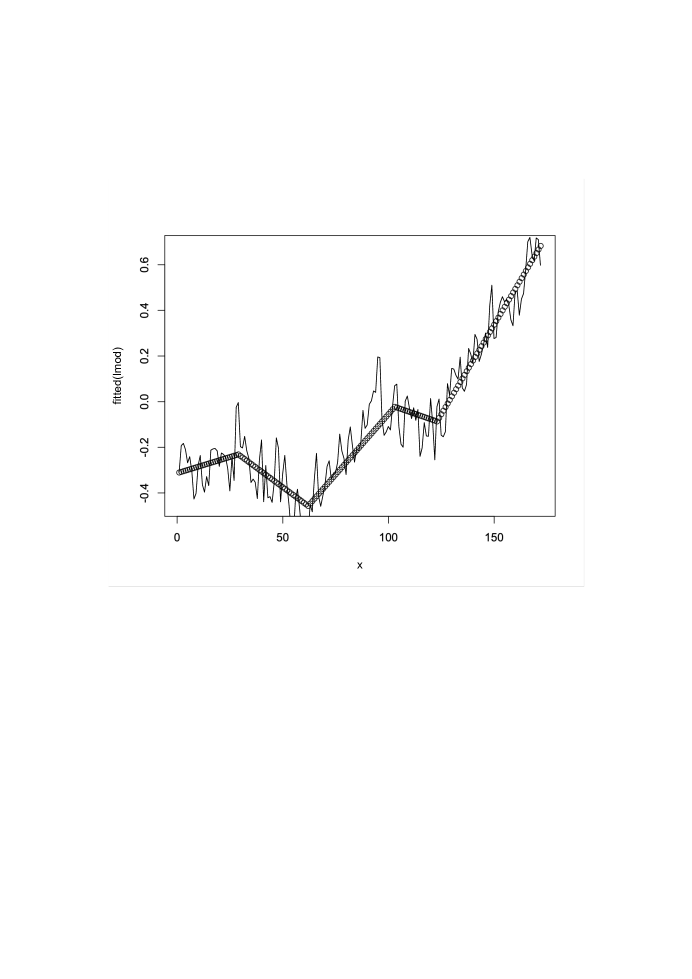
Figure 5: Linear Analysis of Global Ocean Temperature Anomalies.

Example 7: AMO and PDO. These statistics, Atlantic Multidecadal Oscillation and Pacific Decadal Oscillation, monitor changes in ocean currents in the Atlantic and Pacific Oceans, respectively.

There are instrumental data for the AMOC beginning in 1856 and the PDO beginning in 1900. In both cases the data have been recorded monthly, but we average the monthly data to get annual time series with 163 and 118 values, respectively. Since the changes here occur over short time intervals, with relatively flat stretches between changes, we use a model for jump changes. The methods are those described in our previous paper, although now we allow non-zero slopes between change-points and first order autocorrelation.

The entire AMO time series produces an estimated value $\hat{\rho}=0.68$. All methods agree that there is a decrease in the mean in 1901, an increase at 1925, a decrease in about 1963, and the latest increase 1995. A linear analysis incorporating these change-points returns an $R^{2}$ of about 0.72 and an auto-correlation of 0.03, which does not test as different from 0. It seems interesting to observe that the changes in slope detected in the Northern Hemisphere ocean temperature anomalies discussed in the preceding example fall very close to the mid-points of these intervals.

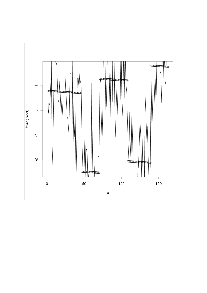
Figure 6: Linear Analysis of AMO Data, with Jump Changes of Level in 1901,1925,1963,1995.

The PDO data are similar, but changes appear to be more frequent, as the name suggests, and a cumulative sum plot appears very noisy. Here, if we estimate $\rho$ by all the observations, we get 0.55 and detect no changes. If we use the observations from 1 to 45, to estimate $\rho$, we get 0.30, and we detect changes in 1947, 1975, 1998, and 2013 by two methods, while the stricter method that uses all possible background intervals detects changes in 1947, 1975, and 2013. A linear analysis with all four detected change-points produces an $R^{2}$ of 0.48 and an estimate for $\rho$ of 0.27.

Example 8: Atmospheric Greenhouse Gases. In view of their connection with global warming, it is interesting to consider atmospheric greenhouse gases. Systematic atmospheric measurements began relatively recently, although reconstructions from surrogate measurements go back centuries. To illustrate our methods, we first consider global average methane emissions for 35 years beginning in 1984, reported at ftp://aftp.cmdl.noaa.gov/products/trends/ch4/.

A linear model without changes shows a positive slope with an $R^{2}$ of 0.95 and an autocorrelation of zero. MS detects a slowing of the rate of increase in 1993 followed by a large increase in 2010. Incorporating these changes into a linear model produces an $R^{2}$ greater than 0.99 and an autocorrelation of zero. The statistic (16) detects the same two changes, although it places the initial decrease about 1996.

Atmospheric measurements of CO₂ begin about 1960 and provide a similar picture. Next we consider 514 years, beginning in 1501, of surrogate measurements of CO₂ provided by the Institute for Atmospheric and Climate Science (IAC) at the ETH-Zürich on the web site www.co2.earth/historical-co2-datasets. Unlike other examples, where changes may be missed because of large variability, the variability in these data (and in the recent atmospheric measurements) is very small. There appear to be many small changes that do not help us to understand large-scale patterns. The statistic MS detects 10 changes, the first in 1575 and the last in 1990. Two changes decrease the slope, while eight increase it. See Figure 8. BIC has a slight preference for a nine change model. The top down statistic (16), which detects essentially the same slope changes, may have some advantages in problems like this one, since it focuses first on large changes; and we can stop looking when we think that adding more changes does not alter our basic insights. Seq does not work well, since it picks out many very small changes that it seems reasonable to ignore.

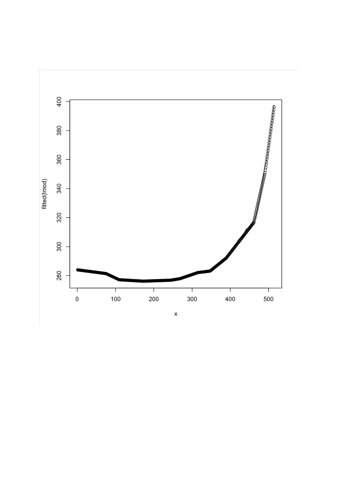
Figure 7: Linear Analysis of reconstructed atmospheric CO2, 1501-2014.

Example 9. Incidents of hate crimes are reported by the United States FBI web site www.fbi.gov from 1996 to 2020. The record is divided into hate crimes against specific, overlapping groups, ethnic, relgious, etc. The largest target of hate crimes is African-Americans. A plot showing slope changes in 2008, 2014, and 2019, detected by (16) with $\rho=0$, is given in Figure 9, where $R^{2}=0.94$, and $\rho$ is estimated to be -0.18. Seq detects only the second slope change. BIC prefers the three change model to a one change model and all two change models. The time series for crimes against Asian-Americans is similar, but the numbers are smaller, so detection more difficult. The time series for all hate crimes is similarly V-shaped, but without the disproportionately large increase between 2019 and 2020.

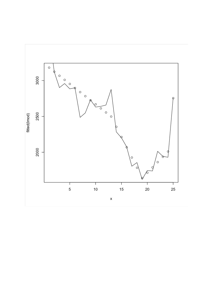
Figure 8: Linear Analysis of Hate Crimes against African-Americans.

Appendix C: Bump Hunting: fixed shape, variable amplitude and scale.

In a variety of problems, the local signal to be detected occurs in a departure from, followed by a return to, a baseline value. In many cases the shape of the local signal arises naturally from the scientific context. An important example is inherited copy number variation, where there is an abrupt increase or decrease from the baseline value of two, which is followed quickly by a return to the baseline (e.g., Zhang et al. (2010)). Other examples are ChIP-Seq, where a shape to expect is roughly triangular or double exponential (e.g., Shin   et al. (2013)) , or differential methylation, where a normal probability density function might be reasonable (cf. Jaffe, et al. (2012a)).

We modify (2) to include a scale paramter $\tau$, to obtain the log likelihood function

$$-.5\sum_{1}^{T}[Y_{u}-\rho Y_{u-1}-\mu_{u}-\sum_{k}\xi_{k}f\{(u-t_{k})/\tau_{k}\}]^{2}.$$ (26)

Here $f$ is a positive, symmetric integrable function, e.g., the square root of (i) a standard normal density function, (ii) a triangular probability density on $[-1,1]$, (iii) a double exponential probability density, or (iv) a uniform probability density function on $[-1/2,1/2]$. Consider the case of at most one bump and assume that the search interval is long enough relative to the scale parameter that it is reasonable to ignore end effects. We define our standardized statistic as above, but we now write it as $Z_{t,\tau}$ to reflect the unknown location $t$ and width $\tau$ of the bump. An approximation to its false positive error probability is given in display (9).

If bumps are sparse, estimation of $\rho$ and $\sigma^{2}$ is relatively easy, since occasional signals do not seriously bias maximum likelihood estimators.

Remarks. (i) The approximation (9) does not apply to case (iv) mentioned above. Because of discontinuities in $f$, a different approximation is required (cf. Fang, Li and Siegmund (2020)). (ii) A serious study of these methods is warranted by the variety of potential applications, some of which involve spatio-temporal random fields. (iii) For some applications it may be reasonable to assume that the underlying process is a Poisson or other point process, which among other effects makes the tail probability of the maximum value of $Z_{t}$ substantially larger, as mentioned in Section 4.

Appendix D: Additional COVID-19 Examples.

Example 10. COVID-19 in Italy. An interesting example of the corona virus is Italy, which had substantial difficulty in controlling the spread of the virus in the early days of the pandemic. Using data for 621 days up to (including) 13 October 2021, we find that (16) with $\rho=0.3$ detects ten slope changes. A linear least squares analysis produces an $R^{2}\approx 0.98$ and an estimate of $\rho$ of 0.67. See Figure 10. We might want to repeat the analysis with this larger value of $\rho$, but the effect seems to be to make the change at observation 356 into a borderline case, which might be omitted, and leave other slope changes essentially as originally detected.

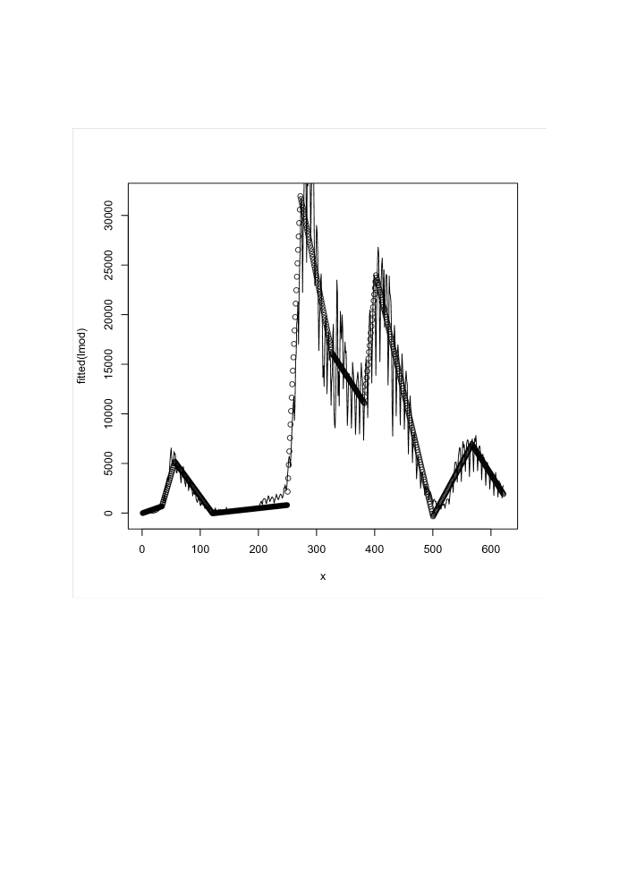
Figure 9: Linear Analysis of COVID-19 Incidence in Italy, 31/01/20-25/08/21.

Example 11. COVID-19 in Hong Kong An extremely well organized and informative web site is

chp-dashboard.geodata.gov.hk/covid-19/en.html

;

Ourworldindata also contains well organized daily incidence data for Hong Kong, although it did not in the early days of the pandemic.

For 579 days from 25/01/2020 to 25/08/2021 all three methods give about the same results. MS produces the best looking broken line, largest $R^{2}$ (about 0.94) and smallest $\rho$ (about 0.35) in the linear analysis. See Figure 11.

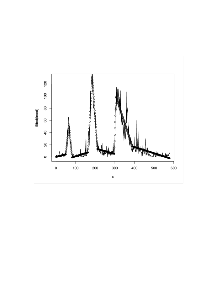
Figure 10: Linear Analysis of COVID-19 Incidence in Hong Kong, 25/01/20-25/08/21.

For daily incidence of COVID-19, it is apparent from Figures 10 and 11 that the variability is much larger when the incidence is large. It does not seem important to deal with this heteroscedasticity because slope changes are also usually much larger when the incidence is large. We have, however, considered the possibilities of transforming the data, say by taking a square root or a logarithm. This rarely seems to have a consequential effect.

Since simple epidemic models suggest that the incidence of an infections disease increases (and decreases) exponentially, one might prefer using a (usually overdispersed) log Poisson linear model. This sometimes produces a visually more appealing plot and in some cases allows one to discard some change-points because the natural curvature of the model substitutes for a slope change in a broken line model.

Appendix E: Threshold Autoregression

As a final illustration of our methods we consider a simple case of Threshold Autoregression, which has been studied in a number of papers by Tong and colleagues.

For a model assume

$$Y_{u}=\mu+\rho Y_{u-1}+\xi Y_{u-1}I\{Y_{u-1}\leq t\}+\epsilon_{u}$$ (27)

To test $\xi=0$, in the notation of Section 2

$$\ell_{\xi}(t)=\sum_{u}(Y_{u}-\mu-\rho Y_{u-1})Y_{u-1}I\{Y_{u-1}\leq t\},$$

and asymptotically under the null hypothesis we have

$$\Psi(t)^{\prime}\sim T(\mathbb{E}(Y;Y\leq t),\mathbb{E}(Y^{2};Y\leq t)),$$

$$\dot{\ell}_{\theta}=(\sum(Y_{u}-\mu-\rho Y_{u-1}),\sum[(Y_{u}-\mu-\rho Y_{u-1})Y_{u-1}],$$

and $A^{-1}$ is the $2\times 2$ matrix with entries $a_{11}=T,\;a_{12}=T\mathbb{E}(Y),\;a_{22}=T\mathbb{E}(Y^{2}),$ where $Y$ denotes the stationary distribution of $Y_{u}$ under the null hypothesis (and the stationarity assumption that $|\rho|<1$). Hence

$$\sigma^{2}(t)\sim T\mathbb{E}(Y^{2};Y\leq t)$$

$$-T[\mathbb{E}^{2}(Y^{2};Y\leq t)+\mathbb{E}(Y^{2})\mathbb{E}^{2}(Y;Y\leq t)-2\mathbb{E}(Y)\mathbb{E}(Y;Y\leq t)\mathbb{E}(Y^{2};Y\leq t)]/{\mathbb{V}}{\mathrm{a}r}(Y).$$ (28)

Let $G(t)=\mathbb{E}(Y^{2};Y\leq t)$, so $\sigma^{2}(t)\sim T[G(t)-\Psi(t)^{\prime}A\Psi(t)].$ Straightforward calculations show that the covariance of the standardized score statistics $Z_{s}$ and $Z_{t}$ are given by $[G(\min(s,t))-\Psi^{\prime}(s)A\Psi(t)]/\sigma(s)\sigma(t).$ Hence locally for small $\delta$

$${\mathbb{C}}{\mathrm{o}v}(Z_{t},Z_{t+\delta})\approx I-(\delta/2)[G-\Psi^{\prime}A\Psi]^{-1}\dot{G},$$

where the functions $G$, $\Psi$ and $\dot{G}$ are evaluated at $t$, and slightly more generally

$${\mathbb{C}}{\mathrm{o}v}[(Z_{t+\delta_{1}},Z_{t+\delta_{2}})|Z_{t}]\approx\min(\delta_{1},\delta_{2})[G-\Psi^{\prime}A\Psi]^{-1}\dot{G}.$$

This allows us to calculate an approximation to $\mathbb{P}\{\max_{t}|Z_{t}|\geq b\}$. The methods of, e.g., Woodroofe (1976) or Yakir (2013) lead after some calculation to

$$\mathbb{P}\{\max_{t_{0}<t<t_{1}}|Z_{t}|>b\}\approx 2b\varphi(b)\int_{t_{0}}^{t_{1}}[\Psi^{\prime}(t)A\dot{\Psi}(t)/\sigma^{2}(t)]dt.$$ (29)

We have evaluated (29) by numerical integration, and the p-values given below come from that evaluation with the observed mean value and standard deviation. We have also implemented an empirical version of this approximation, where the entire computation is based on the appropriately estimated quantities. These two approximations are in rough agreement for our examples, where the p-value is very small. Simulations suggest that the Type I error control of (29) is adequate under the model The power also seems reasonable. In principle, one should learn something from the maximizing point of the statistic $Z_{s}$ relative to the estimated values of $\mu$ and of $\sigma$, but in simulations the maximizing value of shows more variability than we can easily interpret. A calculation similar to that giving (28) indicates that in the case that $\xi\neq 0$ the expected value of $Z_{t}$ is approximately $\xi T^{1/2}\sigma(t)$, as it would be for likelihood theory with standard regularity conditions. This approximation seems relatively stable and suggests a rough approximation for $\xi$ by equating the approximation to the observed value of $\max_{s}Z_{s}$ (or $\min_{s}Z_{s}$).

With a slight modification in principle, but substantially more detailed calculation in application, one can consider higher order autoregressions. Suppose, for example, the model is

$$Y_{u}=\rho_{1}Y_{u-1}+\rho_{2}Y_{u-2}+(\xi_{1}Y_{u-1}+\xi_{2}Y_{u-2})I\{Y_{u-2}\leq t\}+\epsilon_{u}.$$

Now $X_{t}$ is a two-dimensional vector, while $G(t)$, $\Psi(t)$, and $\sigma^{2}(t)=\Sigma_{t},$ say, are $2\times 2$ matrices. An appropriate test statistic has the form $\max_{t}V_{t}^{\prime}\Sigma^{-1}_{t}V_{t}.$ Putting $Z_{t}=\Sigma^{-1/2}V_{t}$, we can control the false positive probability based on the approximation

$$\mathbb{P}\{\max_{t_{0}<t<t_{1}}||Z_{t}||>b\}$$

$$\approx(b^{2}/2)\exp(-b^{2}/2)(2\pi)^{-1}\int_{t_{0}}^{t_{1}}\int_{0}^{2\pi}{\bf e}^{\prime}\Sigma^{-1}_{t}\dot{G}(t){\bf e}d\omega dt+\exp(-b^{2}/2),$$ (30)

where ${\bf e}=(\cos(\omega),\sin(\omega))^{\prime}$, and where $\pi^{-1}$ times the integral over $\omega$ equals the trace of $\Sigma^{-1}_{t}\dot{G}(t)$.

Simulations suggest that the Type I error control of this procedure is adequate under the model. The power also seems reasonable. In principle, one should learn something from the maximizing point of the statistic $Z_{t}$ relative to the estimated values of $\mu$ and of $\sigma$, but in simulations the maximizing value of $t$ shows more variability than we can easily interpret.

Examples. As illustrative applications, we follow Chan and Tong (1990) in considering the Canadian lynx data and Nicholson’s blowfly data. We do not, however, try to give a complete discussion of these well studied data.

The Canadian lynx data consist of annual counts over a 114 year period, which are considered a surrogate for the size of the lynx population. The scientific reasoning behind a two-phase model is the hypothesis that when the lynx population is small, it finds a more than adequate food supply and increases until it reaches a size where the food supply is inadequate, when it then decreases until the cycle begins again. Empirical observations suggest that the decrease in times of food shortage is more rapid than the increase in times of abundance. If we use a first order auto regressive model, these fluctuations suggest a positive autoregressive parameter in times of food abundance, which decreases when there is a food shortage. Although there are clear outliers in the data, which has lead others to consider transformations to shorten the tails, we analyze the original data. Employing the first order autoregressive model with a possible change in the autoregressive parameter, as suggested above yields null estimators of $\mathbb{E}(Y)$ and ${\mathbb{V}}{\mathrm{a}r}(Y)$ of 1538 and 1560, respectively. The maximum value of $Z_{t}$ is 3.89, which occurs at about $t=3500$, and the resulting (two-sided) p-value based on (29) is approximately $0.004$.

Nicholson’s blowfly data (Brillinger, et al. (1980) from the web site

www.stat.berkeley.edu/ brill/blowfly97I.html

,

contains 361 observations in four columns, labeled respectively “births,” “nonemerging,” “emerging,” and “deaths.” The first, third, and fourth columns vary from numbers close to 0 to numbers in the several thousands. The second column typically involves substantially smaller numbers. For the first column. the estimated mean value, autocorrelation, and standard deviation under the null model are 1438, 0.6 and 1670, respectively. The maximum $Z$ value is about 4.73, which occurs for $t\approx 5300.$ The p-value for the hypothesis of no change is approximately $2\times 10^{-4}.$ For “emerging” the maximum $Z$-value is about 5.22, which gives a p-value of about $6\times 10^{-5}.$ For these data the change in the autocorrelation is positive.

References

- Adler and Taylor (2007) R. J. Adler and J. E. Taylor (2007). Random Fields and Geometry Springer-Verlag, New York-Heidelberg-Berlin.
- Arrhenius (1896) S. Arrhenius (1896). On the influence of carbonic acid in the air on the temperature on the ground, Philos. Mag. 41, 237-276.
- Baranowski, Chen, and Fryzlewicz (2019) R. Baranowsk, Yining Chen, and P. Fryzlewicz (2019). Narrowest-over-threshold detection of multiple change-points and change-point-like features J. Roy. Statist. Soc. B 89, 649-672.
- Chan and Tong (1990) K. S. Chan and H. Tong (1990) On likelihood ratio tests for threshold autoregression JRSSB 52, 469-476.
- Davies (1987) R. B Davies (1987). Hypothesis testing when a nuisance parameter is present only under the alternative Biometrika 74, 33-43.
- Fang, Li and Siegmund (2020) X. Fang, J. Li and D. O. Siegmund (2020). Segmentation and estimation of change-point models: false positive control and confidence regions Ann. Statist. 43, 1615–1647.
- Fryzlewicz (2014) P. Fryzlewicz (2014). Wild binary segmentation for multiple change-pont detection. Ann. Statist. 42, 2243–2281.
- Heyde, (1997) C. C. Heyde (1997) Quasi-Likelihood and Its Application Springer-Verlag, New York-Heidelberg-Berlin.
- Jaffe, et al. (2012a) A. E. Jaffe, A. P. Feinberg, R. A. Irizarry, and J T. Leek (2012a). Significance analysis and statistical dissection of variably methylated regions. Biostatistics 13, 166–178.
- Jaffe, et al. (2012b) A. E. Jaffe, P. Murakami, Hwajin Lee, J T. Leek, M. Daniele Fallin, A P. Feinberg, and R. A. Irizarry (2012b). Bump hunting to identify differentially methylated regions in epigenetic epidemiology studies, Int. J. of Epidemiology 41, 200–209.
- Jones, et al. (2012) P. D. Jones, D. H. Lister, T. J. Osborn, C. Harpham, M. Salmon, and C. P. Morice Hemispheric and large-scale land surface air temperature variations: An extesive revision and an update to 2010. J. Geophys. Res. 117 D05127,doi:10.1029/2011JD017139.
- Knowles and Siegmund (1989) M. Knowles and D. Siegmund (1989) On Hotelling’s approach to testing for a nonlinear parameter in regression Int. Statist. Rev. 57 205-220.
- Knowles, Siegmund and Zhang (1991) M. Knowles, D. Siegmund and H. P. Zhang (1991) Confidence regions in semilinear regression Biometrika 79 15-31.
- Krieger, Pollak and Yakir (2003) A. B. Krieger, M. Pollak, and B. Yakir (2003) Surveillance of a simple linear regression J. Amner. Statist. Assoc. 98 456-469.
- Manley (1974) Gordon Manley (1974) Central England temperatures:monthly means 1659 to 1973 Quarterly J. Roy. Meteorological Soc. 100 389-405.
- Muggeo (2016) V. M. R Muggeo (2016) Testing with a nuisance parameter present only under the alternative: a score based approach with application to segmented modeling J. Statistical Computation and Simulation doi: 10.1080/00949655.2016.1149855
- Olshen et al. (2004) A. B. Olshen, E. S. Venkatraman, R. Lucito and M. Wigler (2004). Circular binary segmentation for the analysis of array-based DNA copy number data. Biostatistics 5, 557–572.
- Raftery and Akman (1986) A. E. Raftery and V. E. Akman (1986). Bayesian analysis of a Poisson process with a change-point. Biometrika 73, 85–80.
- Robbins, Gallagher, and Lund (2016) M. W. Robbins, C. M. Gallagher, and R. Lund (2016). A general regression change-point test for time series data, Jour. Amer. Statist. Assoc. 111 670–683.
- Schwartzman et al. (2013) A. Schwartzman, A. Jaffe, Y. Gavrilov, Y. and C. E. Meyer (2013). Multiple testing of local maxima for detection of peaks in ChIP-seq data, Ann. Appl. Statist., 7, 471-494.
- Shin et al. (2013) H. Shin, T. Liu, X. Duan, Y. Zhang, X. S. Liu (2013). Computational methodology for ChIP-seq analysis. Quantitative Biology 1, 54–70.
- Siegmund and Yakir (2000) D. O. Siegmund and B. Yakir (2000). Tail probabilities for the null distribution of scanning statistics. Bernoulli 6, 191–213.
- Siegmund and Worsley (1995) D. O. Siegmund and K. J. Worsley (1995). Testing for a signal with unknown location and scale in a stationary Gaussian random field. Ann. Statist. 23, 608–639.
- Smith and Cook (1980) A. F. M. Smith and D. G. Cook (1980). Strait lines with a change-point: an analysis of some renal transplant data J. Roy. Statist. Soc. Series C 29, 180-189.
- Toms and Lesperance (2003) J. D. Toms and M. L. Lesperance Piecewise regression: a tool for identifying ecological thresholds Ecology 84, 2034-2041.
- Zhang et al. (2010) N. R. Zhang, D. O. Siegmund, H. Ji and J. Z. Li (2010). Detecting simultaneous changepoints in multiple sequences. With supplementary data available online. Biometrika 97, 631–645.

References

- Brillinger, et al. (1980) D. R. Brillinger, J. Guckenheimer, P. Guttorp and G. Oster (1980) Empirical modelling of population time series data: the case of age and density dependent vital rates Lectures on Mathematics in the Life Sciences 13, 65-90 American Math. Soc.
- Chan (1991) K. S. Chan (1991) Percentage points of the likelihood ratio test for threshold autoregression JRSSB 53, 691-696.
- Chan and Tong (1990) K. S. Chan and H. Tong (1990) On likelihood ratio tests for threshold autoregression JRSSB 52, 469-476.
- Church and White (2011) J. A. Church and N. J. White (2011) Sea level rise from the late 19th to the early 21st century Surv. Geophysis. 32, 585-602.
- Jaffe, et al. (2012a) A. E. Jaffe, A. P. Feinberg, R. A. Irizarry, and J T. Leek (2012a). Significance analysis and statistical dissection of variably methylated regions. Biostatistics 13, 166–178.
- Jaffe, et al. (2012b) A. E. Jaffe, P. Murakami, Hwajin Lee, J T. Leek, M. Daniele Fallin, A P. Feinberg, and R. A. Irizarry (2012b). Bump hunting to identify differentially methylated regions in epigenetic epidemiology studies, Int. J. of Epidemiology 41, 200–209.