First-Order Methods for Optimal Experimental Design Problems with Bound Constraints

Abstract

We consider a class of convex optimization problems over the simplex of probability measures. Our framework comprises optimal experimental design (OED) problems, in which the measure over the design space indicates which experiments are being selected. Due to the presence of additional bound constraints, the measure possesses a Lebesgue density and the problem can be cast as an optimization problem over the space of essentially bounded functions. For this class of problems, we consider two first-order methods including FISTA and a proximal extrapolated gradient method, along with suitable stopping criteria. Finally, acceleration strategies targeting the dimension of the subproblems in each iteration are discussed. Numerical experiments accompany the analysis throughout the paper.

1 Introduction

In this paper we consider problems of the following form:

Minimize $$F(\Lambda w),\quad w\in C(X)^{*}$$ (1.1)

s.t. $$w\in\Delta_{C}\cap\mathcal{B}.$$

Here $X$ is a compact subset of $\mathbb{R}^{d}$, and $C(X)^{*}$ is the dual of the space of continuous functions on $X$, which can be represented by signed, finite, regular Borel measures on $X$; see for instance [15, Prop. 7.16] or [34, Thm. 6.19]. The set $\Delta\subset C(X)^{*}$ is the standard simplex of probability measures,

$$\Delta=\{w\in C(X)^{*}\,|\,w\geq 0\text{ and }w(X)=1\}$$

and $\Delta_{C}=C\delta$ for some $C>0$. Moreover, $\Lambda\in\mathcal{L}(C(X)^{*},\mathbb{S}^{n})$ is a bounded linear operator where $\mathbb{S}^{n}$ is the space of symmetric $n$-by-$n$ matrices. Finally, $F:\mathbb{S}^{n}\to\overline{\mathbb{R}}\coloneqq\mathbb{R}\cup\{+\infty\}$ is a proper, convex, lower semi-continuous function.

In the absence of $\mathcal{B}$, problems of type (1.1) arise in the formulation of continuous sensor placement or, more generally, optimal experimental design (OED) problems for parameter identification; see [40, Ch. 3], [32, Ch. 5]. In this setting, $X$ is termed the design space and $w$ is the design measure, which describes the weighted composition of an ensemble of measurements (a complete experiment) from elementary measurements (experiments). In this context, $n$ is the dimension of the space of unknown parameters, and $\Upsilon(x)\in\mathbb{S}^{n}$ denotes the positive-semidefinite Fisher information of the elementary experiment associated with the design point $x$. We assume that $\Upsilon$ depends continuously on $x$, i.e., $\Upsilon\in C(X;\mathbb{S}^{n})$ and that

$$\Lambda w\coloneqq\int_{X}\Upsilon(x)\operatorname{\,d\!}w(x)$$ (1.2)

denotes the total Fisher information matrix (FIM) of the experiment with weight $w\in C(X)^{*}$.

In this paper we focus on OED problems of type (1.1) in the presence of additional bound constraints. Such problems have been discussed before, e.g., in [13, 8, 31, 25, 28] and [14, Chapter 4.3]. Specifically, we consider

$$\mathcal{B}\coloneqq\{w\in C(X)^{*}\,|\,0\leq w(A)\leq\lvert A\rvert\text{ for all Borel sets }A\subset X\},$$ (1.3)

where $\lvert A\rvert$ denotes the Lebesgue measure of $A$. The constraints in (1.3) can represent, among other things, an upper bound on the density of sensors placed in any given subset $A$ of the observation domain $X$. Naturally, we need to assume $0\leq C\leq\lvert X\rvert$ in order for (1.1) to be feasible. Notice that (1.1)–(1.4) is a convex problem.

The presence of $\mathcal{B}$ changes problem (1.1) quite a lot. First of all, (1.3) implies that the Borel measure $w$ is absolutely continuous w.r.t. the Lebesgue measure on $X$. This implies that $w$ possesses a density (Radon–Nikodym derivative) in $L^{1}(X)$ w.r.t. the Lebesgue measure. In a slight abuse of notation, we denote this density also by $w$. Moreover, (1.3) implies that $0\leq w\leq 1$ holds a.e. in $X$ and thus in fact $w$ belongs to $L^{\infty}(X)$.

Second, the structure of optimal solutions of (1.1) depends on whether or not $\mathcal{B}$ is present. In the absence of $\mathcal{B}$, the set of optimal measures contains an element which has sparse support and is, in fact, a non-negative linear combination of at most $n\,(n+1)/2$ Dirac measures. This is a consequence of Carathéodory’s theorem; see for instance [40, Thm. 3.1]. With $\mathcal{B}$ present, the set of optimal measures contains a representer which is of bang-bang type, i.e., $w(x)\in\{0,1\}$ holds a.e. in $X$; see [14, Thm. 4.3.1].

A typical class of design criteria for OED problems is given by

$$F_{q}(I)=\begin{cases}\bigl{(}\frac{1}{n}\operatorname{trace}I^{-q}\bigr{)}^{\frac{1}{q}}&\text{for }q\in(0,\infty),\\ \frac{1}{n}\ln\det I^{-1}&\text{for }q=0\end{cases}$$ (1.4)

for positive definite matrices $I\in\mathbb{S}^{n}$ (denoted by $I\succ 0$); see for instance [20, eq.(4.11)] or [40, eq.(2.17)]. For the sake of simplicity, we omitted a multiplicative constant. Important special cases are the A-criterion ($q=1$), the logarithmic D-criterion ($q=0$) and the E-criterion $F_{\infty}(I)=\max\operatorname{eig}(I^{-1})$ obtained in the limit $q\to\infty$. When $I\in\mathbb{S}^{n}$ is not positive definite, we set $F_{q}(I)\coloneqq+\infty$. Notice that all criteria satisfy the assumptions of being proper and convex functionals on $\mathbb{S}^{n}$. Moreover, all except $F_{\infty}$ are of class $C^{\infty}$ on their domain. Notice that for $I\succ 0$ we have $F_{q}(I)\to(\det I^{-1})^{1/n}$ as $q\searrow 0$, see [20, eq.(4.11)], and thus the criterion $F_{0}$ is not the limit of $F_{q}$ but its logarithm. However it is customary to use the equivalent criterion given in (1.4) in case $q=0$.

There are several classes of numerical approaches to solving (1.1)–(1.4) in the absence of $\mathcal{B}$. An early, so-called additive approach has been presented by [12, 45, Ch. 2.5], which proceeds by taking convex combinations of the current iterate and a particular vertex of the probability simplex $\Delta_{C}$. This idea has been further improved by [26] in order to ensure the sparsity of the solution within each iteration. By contrast, so-called multiplicative algorithms have been introduced for discretized versions of the problem, which modify all weights simultaneously, see [37, 39, 46]. Alternative approaches are obtained by reformulating the problem into a second order cone or semidefinite program, see for instance [36, 1].

We also mention problems which feature binary constraints $\mathcal{B}^{\prime}=\{w\in C(X)^{*}\,|\,w(\{x\})\in\{0,1\}\text{ for all }x\in X\}$. Hence in contrast to $\mathcal{B}$, only Dirac measures are allowed. Examples include so-called exact sensor placement problems, where one seeks to identify the most useful positions for a given number of sensors. Typical algorithms for a discrete versions of this problem are either sequential or of exchange type. Sequential methods insert one sensor at a time, yielding suboptimal solutions; see for instance [27, 43, 16]. Exchange algorithms revisit previously placed sensors and replace a subset of them by unused ones, often heuristically. For more details see [2, Ch. 12], [14, Ch 4.3] or [40, Ch. 7].

An exact approach to discretized exact sensor placement problems of branch-and-bound type, which takes into account the combinatorial nature, is discussed in [41]. It requires the solution of subproblems which are discretized variants of (1.1)–(1.4). In order to solve these subproblems, the authors make use of a simplicial decomposition algorithm, where the inner, so-called restricted master problems, are solved using a multiplicative algorithm. Recently, [11] proposed to replace the latter by FISTA ([4]), which significantly reduced the computational time.

The goal of this paper is to formulate, discuss and numerically compare first-order methods for the solution of (1.1)–(1.4) and its discrete variants. First-order methods are popular for a variety of smooth and non-smooth optimization problems; see for instance [10, 6, 3]. To the best of our knowledge, first-order methods (with or without simplicial decomposition) have not been considered for the solution of optimal experimental design problems with bound constraints $\mathcal{B}$.

For the sake of completeness, we embed (1.1)–(1.4) into a family of regularized problems

Minimize $$F_{q}(\Lambda w)+\frac{\alpha}{2}\lVert w\rVert_{L^{2}(X)}^{2},\quad w\in L^{2}(X)$$ (1.5)

s.t. $$w\in\Delta_{C}\cap\mathcal{B}.$$

with parameter $\alpha\geq 0$. Recall that the fact that the design measure $w$ is sought in $L^{2}(X)$ is not a result of the regularization term but rather a consequence of the bound constraints in $\mathcal{B}$. The case $\alpha>0$ is interesting since the solution $w$ is unique, which is in general not the case for $\alpha=0$. Finally, we are going to shows that a choice of $\alpha>0$ does not jeopardize the sparsity of the optimal design measure, which is an important consideration for the practical realization.

Taking into account that $w$ has a Lebesgue density, the synthesis operator (1.2) can be extended to $\Lambda\in\mathcal{L}(L^{2}(X),\mathbb{S}^{n})$ and it can be written as

$$\Lambda w\coloneqq\int_{X}\Upsilon(x)\,w(x)\operatorname{\,d\!}x.$$ (1.6)

Here it is sufficient to assume $\Upsilon=L^{2}(X;\mathbb{S}^{n})$. For later reference, we note that the Hilbert space adjoint $\Lambda^{*}\in\mathcal{L}(\mathbb{S}^{n},L^{2}(X))$ of $\Lambda$ is given by

$$(\Lambda^{*}P)(x)=P\dprod\Upsilon(x),$$ (1.7)

where $A\dprod B=\operatorname{trace}(A^{\mkern-1.5mu\mathrm{T}}B)$ for matrices of equal size. Moreover, we note that the scaled probability simplex in $L^{2}(X)$ can be written as

$$\Delta_{C}\coloneqq\left\{w\in L^{2}(X)\,\middle|\,w\geq 0\text{ a.e.\ in $X$ and }\int_{X}w\operatorname{\,d\!}x=C\right\}$$ (1.8)

and the bound constraints are

$$\mathcal{B}\coloneqq\left\{w\in L^{2}(X)\,\middle|\,0\leq w\leq 1\text{ a.e.\ in $X$}\right\}.$$ (1.9)

Throughout, we assume that (1.5)–(1.9) is feasible and that

$$0<C<\lvert X\rvert$$ (1.10)

holds, i.e., the solution is neither $w\equiv 0$ nor $w\equiv 1$. Moreover, we assume that there exists $w\in\Delta_{C}\cap\mathcal{B}$ such that $F_{q}(\Lambda w)<\infty$ holds, i.e., there exists at least one feasible experiment which yields a positive definite Fisher information matrix.

Proposition 1.1 (Existence of a solution).

Problem (1.5)–(1.9) is solvable. In case $\alpha>0$, the solution is unique.

Proof 1.2.

The set of attainable Fisher information matrices $\Lambda(\Delta_{C}\cap\mathcal{B})$ is bounded since $\Delta_{C}\cap\mathcal{B}$ is bounded in $L^{2}(X)$ and $\Lambda\in\mathcal{L}(L^{2}(X),\mathbb{S}^{n})$ is continuous. It is easy to see that the objective in (1.5) is bounded below on $\Delta_{C}\cap\mathcal{B}$ since the set of . Consequently, a direct proof based on a minimizing sequence is applicable. The uniqueness of $w$ in case $\alpha>0$ follows from the uniform convexity of the objective in this case.

The structure of the paper is as follows. In Section 2 we investigate necessary and sufficient optimality conditions for the family of convex problems (1.5)–(1.9). A discrete version of the problem is considered in Section 3. In Section 4 we compare the performance of two first-order methods using two numerical experiments. Specifically, we discuss FISTA ([4]) and the proximal extrapolated gradient method from [22]. In Section 5 we discuss the embedding of the methods considered into a simplicial decomposition acceleration, which features subproblems of reduced dimension and significantly improves the performance.

A result which may be of independent interest is an efficient algorithm for the orthogonal projection (w.r.t. an inner product given by $\operatorname{diag}(e_{i})$) onto the restricted simplex

$$\left\{w\in\mathbb{R}^{m}\,\middle|\,0\leq w_{i}\leq 1\text{ for all }i=1,\ldots,m\text{ and }\sum_{i=1}^{m}e_{i}\,w_{i}=C\right\}.$$

The algorithm is given as Algorithm 1 and its correctness is proved in Theorem 3.5.

2 Optimality Conditions

In this section we investigate necessary and sufficient optimality conditions for problem (1.5)–(1.9), which can be equivalently cast in the following typical form for convex optimization problems:

$$\text{Minimize}\quad F_{q}(\Lambda w)+G(w)+H_{\alpha}(w),\quad w\in L^{2}(X).$$ (2.1)

Here we set

$$G(w)\coloneqq I_{\Delta_{C}\cap\mathcal{B}}(w)\quad\text{and}\quad H_{\alpha}(w)\coloneqq\frac{\alpha}{2}\lVert w\rVert_{L^{2}(X)}^{2}$$ (2.2)

and $I_{\Delta_{C}\cap\mathcal{B}}$ denotes the indicator function (in the sense of convex analysis) of the set $\Delta_{C}\cap\mathcal{B}\subset L^{2}(X)$. We recall that we assume (1.10) throughout.

Both $L^{2}(X)$ and $\mathbb{S}^{n}$, endowed with their inner products $\int_{X}w\,v\operatorname{\,d\!}x$ and $P\dprod Q\coloneqq\operatorname{trace}(P^{\mkern-1.5mu\mathrm{T}}Q)$, respectively, are Hilbert spaces and we identify them with their duals via the respective Riesz isomorphisms. Notice that $P\dprod P=\lVert P\rVert_{F}^{2}$ holds, where $\lVert\cdot\rVert_{F}$ is the Frobenius norm of matrices.

Before we present optimality conditions for (1.5)–(1.9), we relate the $L^{2}(X)$-orthogonal projection $\operatorname{proj}_{\Delta_{C}\cap\mathcal{B}}$ to the projection onto $\mathcal{B}$. The latter is simply

$$\operatorname{proj}_{\mathcal{B}}(f)=\max\{\min\{f,1\},0\}.$$

The following result shows that projection onto $\Delta_{C}\cap\mathcal{B}$ is obtained by projection onto $\mathcal{B}$ after an appropriate constant shift of the argument.

Lemma 2.1.

Let $f\in L^{2}(X)$.

1. Suppose that $v=\operatorname{proj}_{\Delta_{C}\cap\mathcal{B}}(f)$ holds. Then there exists $\zeta\in\mathbb{R}$ such that

   $$v=\operatorname{proj}_{\mathcal{B}}(f-\zeta)\quad\text{and}\quad\int_{X}v\operatorname{\,d\!}x=C$$ (2.3)

   holds.

2. Conversely, suppose that $(v,\zeta)\in L^{2}(X)\times\mathbb{R}$ satisfies (2.3), then $v=\operatorname{proj}_{\Delta_{C}\cap\mathcal{B}}(f)$.

Proof 2.2.

We utilize that $v=\operatorname{proj}_{\Delta_{C}\cap\mathcal{B}}(f)$ is characterized by the necessary and sufficient optimality condition

$$(v-f\,,\,w-v)_{L^{2}(X)}\geq 0\quad\text{for all }w\in\Delta_{C}\cap\mathcal{B}, *$$ ()

see for instance [9, Ch. II, eq.(2.17)]. Part $(a)$: Let us define

$$\mathbb{R}\ni\zeta\mapsto a(\zeta)\coloneqq\int_{X}\operatorname{proj}_{\mathcal{B}}(f-\zeta)\operatorname{\,d\!}x\in\mathbb{R}.$$

First we prove that there exists $\zeta\in\mathbb{R}$ such that the equation $a(\zeta)=C$ is solvable. Indeed, it is easy to see that $a(\zeta)$ is Lipschitz with constant $\lvert X\rvert^{1/2}$ and monotone decreasing. Moreover, $\lim_{\zeta\to\infty}a(\zeta)=0$ and $\lim_{\zeta\to-\infty}a(\zeta)=\lvert X\rvert$ hold, and thus $a(\zeta)=C$ is solvable in view of assumption (1.10).

Define $\bar{v}\coloneqq\operatorname{proj}_{\mathcal{B}}(f-\zeta)$. In order to verify that $\bar{v}=v$ holds, it is necessary and sufficient to prove that ($*$ ‣ 2.2) is verified with $v$ replaced by $\bar{v}$. To this end, $w\in\Delta_{C}\cap\mathcal{B}$ be arbitrary. Then

$$\left(\bar{v}-f\,,\,w-\bar{v}\right)_{L^{2}(X)}$$

$$=\left(\operatorname{proj}_{\mathcal{B}}(f-\zeta)-f\,,\,w-\bar{v}\right)_{L^{2}(X)}\quad\text{by definition of $\bar{v}$}$$

$$=\left(\operatorname{proj}_{\mathcal{B}}(f-\zeta)-(f-\zeta)\,,\,w-\bar{v}\right)_{L^{2}(X)}\quad\text{since $\int_{X}\bar{v}\operatorname{\,d\!}x=\int_{X}w\operatorname{\,d\!}x=C$}$$

$$=\int_{\mathchoice{\makebox[0.0pt][l]{$\displaystyle\vphantom{\hskip 42.67912pt}{\{x\in X\,|\,f-\zeta\leq 0\}}$}}{\makebox[0.0pt][l]{$\textstyle\vphantom{\hskip 42.67912pt}{\{x\in X\,|\,f-\zeta\leq 0\}}$}}{\makebox[0.0pt][l]{$\scriptstyle\vphantom{\hskip 42.67912pt}{\{x\in X\,|\,f-\zeta\leq 0\}}$}}{\makebox[0.0pt][l]{$\scriptscriptstyle\vphantom{\hskip 42.67912pt}{\{x\in X\,|\,f-\zeta\leq 0\}}$}}}-(f-\zeta)\,(w-0)\operatorname{\,d\!}x+\int_{\mathchoice{\makebox[0.0pt][l]{$\displaystyle\vphantom{\hskip 42.67912pt}{\{x\in X\,|\,f-\zeta\geq 1\}}$}}{\makebox[0.0pt][l]{$\textstyle\vphantom{\hskip 42.67912pt}{\{x\in X\,|\,f-\zeta\geq 1\}}$}}{\makebox[0.0pt][l]{$\scriptstyle\vphantom{\hskip 42.67912pt}{\{x\in X\,|\,f-\zeta\geq 1\}}$}}{\makebox[0.0pt][l]{$\scriptscriptstyle\vphantom{\hskip 42.67912pt}{\{x\in X\,|\,f-\zeta\geq 1\}}$}}}(1-(f-\zeta))\,(w-1)\operatorname{\,d\!}x.$$

Since $0\leq w\leq 1$ holds, both integrands are non-negative, which proves the claim.

Part $(b)$: Suppose that $(v,\zeta)\in L^{2}(X)\times\mathbb{R}$ satisfies (2.3). By the same argument as above (with $v$ in place of $\bar{v}$) we obtain that ($*$ ‣ 2.2) holds.

We are now in the position to prove necessary and sufficient optimality conditions for the problem (1.5)–(1.9), or equivalently, (2.1)–(2.2). Notice that the symbol $\nabla$ denotes the gradient w.r.t. the inner products in $L^{2}(X)$ and $\mathbb{S}^{n}$, respectively.

Theorem 2.3 (Necessary and sufficient optimality conditions).

1. $w\in L^{2}(X)$ solves (2.1)–(2.2) if and only if

   $$0\in\Lambda^{*}\nabla F_{q}(\Lambda w)+\alpha\,w+\partial G(w)$$ (2.4)

   holds.

2. Suppose $w\in L^{2}(X)$ fulfills (2.4). Then there exists $\zeta\in\mathbb{R}$ such that $(w,\zeta)$ fulfills

   $$w=\operatorname{proj}_{\mathcal{B}}\bigl{(}(1-\alpha)w-\Lambda^{*}\nabla F_{q}(\Lambda w)-\zeta\bigr{)}\quad\text{a.e.\ in }X,$$ (2.5a)

   $$\int_{X}w\operatorname{\,d\!}x=C.$$ (2.5b)

   Conversely if $(w,\zeta)\in L^{2}(X)\times\mathbb{R}$ fulfills (2.5), then $w$ solves (2.1)–(2.2).

3. Suppose that $\alpha=0$ holds and that $w\in L^{2}(X)$ solves (2.1)–(2.2), i.e., $w$ fulfills (2.4). Then there exists another optimal $\bar{w}\in L^{2}(X)$ and a measurable set $M\subset X$ such that

   $$\bar{w}=1\quad\text{a.e.\ in $M$},\quad\bar{w}=0\quad\text{a.e.\ in $X\setminus M$}.$$ (2.6)

We refer to $\bar{w}$ as in (2.6) as a solution of bang-bang type.

Proof 2.4.

Part $(a)$: It is clear that $w\in L^{2}(X)$ solves (2.1) if and only if $0\in\partial(F(\Lambda w)+(G+H_{\alpha})(w))$ holds; see for instance [47, Thm. 2.5.7]. Since we assumed that there exists $w\in\Delta_{C}\cap\mathcal{B}$ with $F_{q}(\Lambda w)<\infty$, and since $(F_{q}\circ\Lambda)(w)$ is continuous at every $w\in L^{2}(X)$ with $\Lambda w\succ 0$, we can apply [47, Thm. 2.8.7 (iii)] and [9, Ch. I, Prop. 5.6] to obtain that the necessary and sufficient optimality conditions of (2.1) They can be written as

$$0\in\Lambda^{*}\nabla F_{q}(\Lambda w)+\nabla H_{\alpha}(w)+\partial G(w)=\Lambda^{*}\nabla F_{q}(\Lambda w)+\alpha\,w+\partial G(w),$$

which is (2.4).

Part $(b)$: We prove this statement by virtue of the following:

$$0\in\Lambda^{*}\nabla F_{q}(\Lambda w)+\alpha\,w+\partial G(w)$$ (2.4)

$$\Leftrightarrow\quad (1-\alpha)w-\Lambda^{*}\nabla F_{q}(\Lambda w)\in\bigl{(}\operatorname{id}+\partial G\bigr{)}(w) *$$ ()

$$\Leftrightarrow\quad w=\bigl{(}\operatorname{id}+\partial G\bigr{)}^{-1}\bigl{(}(1-\alpha)w-\Lambda^{*}\nabla F_{q}(\Lambda w)\bigr{)} **$$ ()

$$\Leftrightarrow\quad w=\operatorname{proj}_{\Delta_{C}\cap\mathcal{B}}\bigl{(}(1-\alpha)w-\Lambda^{*}\nabla F_{q}(\Lambda w)\bigr{)}. ** *$$ ()

The equivalence of (2.4) and ($*$ ‣ 2.4) is clear. The equivalence of ($*$ ‣ 2.4) and ($**$ ‣ 2.4) follows since $\partial G$ is maximally monotone; see for instance [24, 33]. The equivalence of ($**$ ‣ 2.4) and ($**$$*$ ‣ 2.4) follows since $G$ is the indicator function of $\Delta_{C}\cap\mathcal{B}$.

Now if $w\in L^{2}(X)$ fulfills (2.4) and thus ($**$$*$ ‣ 2.4), then Lemma 2.1 part $(a)$ implies the existence of $\zeta$ such that (2.5) holds. Conversely, if $(w,\zeta)\in L^{2}(X)\times\mathbb{R}$ fulfills (2.5), then Lemma 2.1 part $(b)$ shows that $w$ also solves ($**$$*$ ‣ 2.4) and thus also (2.4).

Part $(c)$: The statement follows directly from [44, Thm. 1].

We continue to derive further properties following from the optimality conditions in Theorem 2.3. The following corollary provides a pointwise relation between an optimal $w\in L^{2}(X)$ and $\Lambda^{*}\nabla F_{q}(\Lambda w)\in L^{2}(X)$. This allows us to define, on the one hand, a convenient stopping criterion. On the other hand, it can be used to deduce a certain spatial regularity of an optimal weight $w$, provided that $\Upsilon$ is more regular than $L^{2}(X;\mathbb{S}^{n})$ and belongs, e.g., to the Hölder class $C^{0,\lambda}$ or Sobolev class $W^{1,p}$.

Corollary 2.5 (Further properties of optimal solutions).

1. Condition (2.5a) for $(w,\zeta)$ is equivalent to the existence of a partion $X_{0}\mathbin{\mathaccent 0{\cdot}\cup}X_{01}\mathbin{\mathaccent 0{\cdot}\cup}X_{1}=X$ such that

   $$\left\{\begin{aligned} w(x)=0\text{ and }&-\left(\Lambda^{*}\nabla F_{q}(\Lambda w)\right)(x)&&\leq\zeta&&\quad\text{a.e.\ in }X_{0}\\ 0<{}w(x)<1\text{ and }&-\left(\Lambda^{*}\nabla F_{q}(\Lambda w)\right)(x)-\alpha\,w(x)&&=\zeta&&\quad\text{a.e.\ in }X_{01}\\ w(x)=1\text{ and }&-\left(\Lambda^{*}\nabla F_{q}(\Lambda w)\right)(x)-\alpha&&\geq\zeta&&\quad\text{a.e.\ in }X_{1}\end{aligned}\right\}$$ (2.7)

2. Suppose $\alpha>0$ and $w\in L^{2}(X)$ fulfills (2.4). Then there exists $\zeta\in\mathbb{R}$ such that $(w,\zeta)$ fulfills

   $$w=\operatorname{proj}_{\mathcal{B}}\left(-\alpha^{-1}\Lambda^{*}\nabla F_{q}(\Lambda w)-\zeta\right)\quad\text{a.e.\ in }X,$$ (2.8a)

   $$\int_{X}w\operatorname{\,d\!}x=C.$$ (2.8b)

   Conversely if $(w,\zeta)\in L^{2}(X)\times\mathbb{R}$ fulfills (2.5), then $w$ solves (2.1)–(2.2).

3. Suppose $\alpha>0$ and $\Upsilon\in C^{0,\lambda}(X;\mathbb{S}^{n})$ for some $\lambda\in[0,1]$. Then the optimal solution (2.1)–(2.2) satisfies $w\in C^{0,\lambda}(X)$.

4. Suppose $\alpha>0$ and $\Upsilon\in W^{1,p}(X;\mathbb{S}^{n})$ for some $p\in[1,\infty]$. Then the optimal solution (2.1)–(2.2) satisfies $w\in W^{1,p}(X)$.

Proof 2.6.

Part $(a)$: First we consider that $w\in L^{2}(X)$ fulfills (2.5a). Clearly $w\in\mathcal{B}$ implies the existence of a partition of $X$ such that

$$X_{0} =\{x\in X\,|\,w(x)=0\text{ a.e.}\},$$

$$X_{01} =\{x\in X\,|\,0<w(x)<1\text{ a.e.}\},$$

$$X_{1} =\{x\in X\,|\,w(x)=1\text{ a.e.}\}.$$

It remains to prove the claims for $\left(\Lambda^{*}\nabla F_{q}(\Lambda w)\right)(x)$ in (2.7) on each of these subsets of $X$.

For $x\in X_{0}$, (2.5a) implies

$$0 \geq(1-\alpha)\,w(x)-\left(\Lambda^{*}\nabla F_{q}(\Lambda w)\right)(x)-\zeta$$

$$\Leftrightarrow 0 \geq-\left(\Lambda^{*}\nabla F_{q}(\Lambda w)\right)(x)-\zeta$$

$$\Leftrightarrow \zeta \geq-\left(\Lambda^{*}\nabla F_{q}(\Lambda w)\right)(x)$$

For $x\in X_{01}$, we have $0<w(x)<1$ and (2.5a) implies

$$w(x) =(1-\alpha)\,w(x)-\left(\Lambda^{*}\nabla F_{q}(\Lambda w)\right)(x)-\zeta$$

$$\Leftrightarrow \zeta =-\left(\Lambda^{*}\nabla F_{q}(\Lambda w)\right)(x)-\alpha\,w(x).$$

For $x\in X_{1}$, the proof is analogous to the case $x\in X_{0}$.

Now conversly we assume that a partition of $X$ exists which fulfills (2.7). By plugging in the corresponding relations for each subset of this partition, (2.5a) can be checked easily.

Part $(b)$: Similarily to the proof of Theorem 2.3 part $(b)$ we prove this statement by virtue of the following:

$$0\in\Lambda^{*}\nabla F_{q}(\Lambda w)+\alpha\,w+\partial G(w)$$ (2.4)

$$\Leftrightarrow\quad \alpha^{-1}\Lambda^{*}\nabla F_{q}(\Lambda w)\in\bigl{(}\operatorname{id}+\alpha^{-1}\partial G\bigr{)}(w)$$

$$\Leftrightarrow\quad w=\bigl{(}\operatorname{id}+\alpha^{-1}\partial G\bigr{)}^{-1}\bigl{(}\alpha^{-1}\Lambda^{*}\nabla F_{q}(\Lambda w)\bigr{)}$$

$$\Leftrightarrow\quad w=\operatorname{proj}_{\Delta_{C}\cap\mathcal{B}}\left(\alpha^{-1}\Lambda^{*}\nabla F_{q}(\Lambda w)\right).$$

The proof is concluded by the same arguments as in the proof of Theorem 2.3 part $(b)$ and the observation that the indicator function $G$ is invariant under scaling.

Part $(c)$: Recalling (2.8a) and the representation (1.7) of $\Lambda^{*}$, we have

$$w=\operatorname{proj}_{\mathcal{B}}\left(-\alpha^{-1}\Lambda^{*}\nabla F_{q}(\Lambda w)-\zeta\right)\quad\text{a.e.\ in }X.$$

Suppose now that $\Upsilon\in C^{0,\lambda}(X;\mathbb{S}^{n})$ holds, then $-\nabla F_{q}(\Lambda w)\colon\Upsilon(x)$ belongs to $C^{0,\lambda}(X;\mathbb{R})$. Since $\operatorname{proj}_{\mathcal{B}}(\cdot)$ preserves the class of Hölder continuous functions, the claim follows.

Part $(d)$: Similarly as in part $(c)$, this result follows from the Stampacchia lemma; see for instance [21, Theorem A.1].

Notice that (2.7) implies the sparsity of the optimal weight $w$. This property is reminiscent of optimal control problems with sparsity promoting $L^{1}$-norm objectives; see for instance [38, Section 2] and [7, Remark 3.3].

For practical purposes, we also discuss a relaxed version of the optimality conditions (2.4).

Lemma 2.7 (Relaxed optimality conditions).

Let $\varepsilon>0$. The following statements are equivalent:

1. $w\in L^{2}(X)$ solves the relaxed optimality conditions

   $$y\in\Lambda^{*}\nabla F_{q}(\Lambda w)+\alpha\,w+\partial G(w)$$ (2.9)

   with some $y\in L^{\infty}(X)$ satisfying $\lVert y\rVert_{L^{\infty}(X)}\leq\varepsilon$.

2. There exists $w\in\Delta_{C}$ and $\zeta\in\mathbb{R}$ as well as a partition $X_{0}\mathbin{\mathaccent 0{\cdot}\cup}X_{01}\mathbin{\mathaccent 0{\cdot}\cup}X_{1}=X$ such that

   $$\left\{\begin{aligned} w(x)={}&0\text{ and }&&&&&&\hbox{\multirowsetup$\;\;\text{a.e.\ in }X_{0}$}\\ &&&-\left(\Lambda^{*}\nabla F_{q}(\Lambda w)\right)(x)&&\leq\zeta+\varepsilon\\ 0<w(x)<{}&1\text{ and }&&&&&&\hbox{\multirowsetup$\;\;\text{a.e.\ in }X_{01}$}\\ &\zeta-\varepsilon\leq&&-\left(\Lambda^{*}\nabla F_{q}(\Lambda w)\right)(x)-\alpha\,w(x)&&\leq\zeta+\varepsilon\\ w(x)={}&1\text{ and}&&&&&&\hbox{\multirowsetup$\;\;\text{a.e.\ in }X_{1}$}\\ &\zeta-\varepsilon\leq&&-\left(\Lambda^{*}\nabla F_{q}(\Lambda w)\right)(x)-\alpha\end{aligned}\right\}$$ (2.10)

Proof 2.8.

Similarly as in the proof of Theorem 2.3 part $(b)$ one can show that if $w\in L^{2}(X)$ fulfills (2.9), then there exists $\zeta\in\mathbb{R}$ such that $(w,\zeta)$ verifies

$$w=\operatorname{proj}_{\mathcal{B}}\left((1-\alpha)w+y-\Lambda^{*}\nabla F_{q}(\Lambda w)-\zeta\right)\quad\text{a.e.\ in }X,$$ (2.11a)

$$\int_{X}w\operatorname{\,d\!}x=C.$$ (2.11b)

Conversely, if $(w,\zeta)$ fulfills (2.11), then $w$ also fulfills (2.9).

Analogously to Corollary 2.5 part $(a)$, we find that (2.11a) for $(w,\zeta)$ is equivalent to the existence of a partition $X_{0}\mathbin{\mathaccent 0{\cdot}\cup}X_{01}\mathbin{\mathaccent 0{\cdot}\cup}X_{1}=X$ such that

$$\left\{\begin{aligned} w(x)=0\text{ and }&-\left(\Lambda^{*}\nabla F_{q}(\Lambda w)\right)(x)&&\leq\zeta-y&&\quad\text{a.e.\ in }X_{0}\\ 0<{}w(x)<1\text{ and }&-\left(\Lambda^{*}\nabla F_{q}(\Lambda w)\right)(x)-\alpha\,w(x)&&=\zeta-y&&\quad\text{a.e.\ in }X_{01}\\ w(x)=1\text{ and }&-\left(\Lambda^{*}\nabla F_{q}(\Lambda w)\right)(x)-\alpha&&\geq\zeta-y&&\quad\text{a.e.\ in }X_{1}\end{aligned}\right\}$$ (2.12)

It remains to prove that $(w,\zeta)$ fulfills (2.12) for $\lVert y\rVert_{L^{\infty}(X)}\leq\varepsilon$ if and only if $(w,\zeta)$ fulfills (2.10). Suppose first that (2.12) holds for some $y$ with $\lVert y\rVert_{L^{\infty}(X)}\leq\varepsilon$. Then clearly (2.10) holds. Conversely, suppose that (2.10) holds and choose

$$y\coloneqq\begin{cases}-\varepsilon&\text{ on }X_{0},\\ -\left(\Lambda^{*}\nabla F_{q}(\Lambda w)\right)-\zeta-\alpha\,w&\text{ on }X_{01},\\ \varepsilon&\text{ on }X_{1}.\end{cases}$$

By (2.10), we have $\lVert y\rVert_{L^{\infty}(X)}\leq\varepsilon$. This shows (2.12).

We conclude this section by providing the formula for the gradients of the design criteria $F_{q}$ from (1.4). Its proof can be found, e.g., in [30, eqs. (51) and (110)].

Lemma 2.9.

The gradient of $F_{q}$ at $I\in\mathbb{S}^{n}$ such that $I\succ 0$ is given by

$$\nabla F_{q}(I)=\begin{cases}-(\frac{1}{n})^{\frac{1}{q}}(\operatorname{trace}I^{-q})^{\frac{1}{q}-1}\,I^{-q-1}&\text{for }q\in(0,\infty),\\ -\frac{1}{n}I^{-1}&\text{for }q=0.\end{cases}$$ (2.13)

3 Discretization by Piecewise Constants

In this section we discuss the discretization of the design space $X$ and the design density $w\in L^{2}(X)$. Suppose that $X$ can be discretized into a finite number $m$ of compact polyhedra (cells) $(E_{i})_{i=1,\dots,m}$ of dimension $d$, whose interiors do not intersect. Based on this discretization, $w$ is assumed to be $DG_{0}$, i.e., constant on each $E_{i}$. We write

$$w(x)=\sum_{i=1}^{m}w_{i}\,\chi_{E_{i}}(x)$$

where $\chi_{E_{i}}$ denotes the indicator function of cell $E_{i}$. We endow the space $\mathbb{R}^{m}$ of coefficients of $w$ with the appropriate inner product represented by the matrix

$$M\coloneqq\operatorname{diag}(\lvert E_{1}\rvert,\ldots,\lvert E_{m}\rvert),$$

where $\lvert E_{i}\rvert$ denotes the volume of the $i$-th cell. We associate with each cell the elementary experiment $\Upsilon_{i}$ whose FIM is given by some approximation of the average FIM $\int_{E_{i}}\Upsilon(\cdot)\operatorname{\,d\!}x/\lvert E_{i}\rvert$. When $\Upsilon\in C^{0}(X;\mathbb{S}^{n})$, we can simply take $\Upsilon_{i}=\Upsilon(x_{i})$, where $x_{i}$ is the midpoint of $E_{i}$. This is our method of choice for the numerical experiments in Sections 4 and 5 .

Consequently, we represent the synthesis operator $\Lambda:\mathbb{R}^{m}\to\mathbb{S}^{n}$ as

$$\Lambda w=\sum_{i=1}^{m}\Upsilon_{i}\,\lvert E_{i}\rvert\,w_{i}\in\mathbb{S}^{n}.$$ (3.1)

Its Hilbert space adjoint $\Lambda^{*}:\mathbb{S}^{n}\to\mathbb{R}^{m}$ (w.r.t. the $M$-inner product in $\mathbb{R}^{m}$) is then given by

$$[\Lambda^{*}P]_{i}=P\colon\Upsilon_{i},\quad i=1,\ldots,m.$$ (3.2)

The bound constraints are now written as

$$\mathcal{B}\coloneqq[0,1]^{m}=\{w\in\mathbb{R}^{m}\,|\,0\leq w_{i}\leq 1\text{ for all }i=1,\ldots,m\}$$ (3.3)

and the total mass constraint becomes

$$\Delta_{C}\coloneqq\left\{w\in\mathbb{R}^{m}\,\middle|\,w\geq 0\text{ and }\sum_{i=1}^{m}\lvert E_{i}\rvert\,w_{i}=C\right\}.$$ (3.4)

Hence the discrete version of problem (1.5)–(1.9) can be cast as

Minimize $$F_{q}(\Lambda w)+\frac{\alpha}{2}\lVert w\rVert_{M}^{2},\quad w\in\mathbb{R}^{m}$$ (3.5)

s.t. $$w\in\Delta_{C}\cap\mathcal{B}.$$

Evaluation of $\operatorname{proj}_{\Delta_{C}\cap\mathcal{B}}(\cdot)$

The orthogonal projection w.r.t. the $M$-inner product onto the constraint set $\Delta_{C}\cap\mathcal{B}$ is an essential ingredient in all forthcoming algorithms. We begin by stating a discrete version of Lemma 2.1 without proof.

Lemma 3.1.

Let $f\in\mathbb{R}^{m}$.

1. Suppose that $v=\operatorname{proj}_{\Delta_{C}\cap\mathcal{B}}(f)$ holds. Then there exists $\zeta\in\mathbb{R}$ such that

   $$v=\operatorname{proj}_{\mathcal{B}}(f-\zeta)\quad\text{and}\quad\sum_{i=1}^{m}\lvert E_{i}\rvert\,v_{i}=C$$ (3.6)

   holds.

2. Conversely, suppose that $(v,\zeta)\in\mathbb{R}^{m}\times\mathbb{R}$ satisfies (3.6), then we have $v=\operatorname{proj}_{\Delta_{C}\cap\mathcal{B}}(f)$.

Here $f-\zeta$ denotes the vector with components $f_{i}-\zeta$. We denote a solution of (3.6) by $(v^{*},\zeta^{*})$. Notice that $v^{*}$ is unique but in general this does not hold for $\zeta^{*}$.

In the remainder of this section we describe an efficient algorithm to evaluate $\operatorname{proj}_{\Delta_{C}\cap\mathcal{B}}(f)$. Without loss of generality, we assume that the entries of $f$ are sorted in descending order. In order to facilitate the notation, we introduce a number of abbreviations, where $v\in\mathbb{R}^{m}$, $\zeta\in\mathbb{R}$ and $k,\ell\in\{1,\ldots,m\}$ are arbitrary:

$$\text{nnz}(v) \coloneqq\bigl{\lvert}\{v_{i}\,|\,i\in\{1,\dots,m\}\text{ and }v_{i}>0\}\bigr{\rvert} \text{\#non-zeros in $v$},$$

$$\text{neo}(v) \coloneqq\bigl{\lvert}\{v_{i}\,|\,i\in\{1,\dots,m\}\text{ and }v_{i}=1\}\bigr{\rvert} \text{\#ones in $v$},$$

$$k^{*} \coloneqq\text{nnz}(v^{*})\quad\text{and}\quad\ell^{*}\coloneqq\text{neo}(v^{*}) \text{\#non-zeros, ones in $v^{*}$},$$

$$\mathbb{R}\ni\zeta\mapsto P(\zeta) \coloneqq\operatorname{proj}_{\mathcal{B}}(f-\zeta)\in\mathbb{R}^{m},$$

$$\mathbb{R}^{m}\ni v\mapsto W(v) \coloneqq\sum_{i=1}^{m}\lvert E_{i}\rvert v_{i}\in\mathbb{R}.$$ (3.7)

Notice that once the optimal number of ones $\ell^{*}$ and non-zeros $k^{*}$ are known, the evaluation of the shift $\zeta^{*}$ and thus $v^{*}$ becomes trivial. Indeed, the total weight constraint reads

$$\sum_{i=1}^{\ell^{*}}\lvert E_{i}\rvert+\sum_{i=\ell^{*}+1}^{k^{*}}(f_{i}-\zeta^{*})\,\lvert E_{i}\rvert=C.$$ (3.8)

The solution of this constraint w.r.t. $\zeta$ leads to the definition of the following function,

$$\zeta(k,\ell)\coloneqq\begin{cases}\displaystyle\left(\sum_{i=\ell+1}^{k}\lvert E_{i}\rvert\right)^{-1}\left(\sum_{i=1}^{\ell}\lvert E_{i}\rvert+\sum_{i=\ell+1}^{k}\lvert E_{i}\rvert\,f_{i}-C\right)&\text{if }k>\ell,\\ f_{k}-1&\text{if }k=\ell,\end{cases}$$ (3.9)

for $1\leq\ell\leq k\leq m$. The second case selects the largest possible value of $\zeta$ compatible with the assumption $k=\ell$, i.e., that all positive entries of $\operatorname{proj}_{\mathcal{B}}(f-\zeta(k,\ell))$ are indeed equal to one.

Before we present the idea to evaluate $v^{*}=\operatorname{proj}_{\Delta_{C}\cap\mathcal{B}}(f)$ efficiently, we characterize the (non-)uniqueness of $\zeta^{*}$.

Lemma 3.2.

1. Suppose that $\ell^{*}=k^{*}$ holds. Then $f_{k^{*}+1}\leq f_{k^{*}}-1$. Moreover, (3.6) is valid if and only if $\zeta^{*}\in[f_{k^{*}+1},f_{k^{*}}-1]$.

2. Suppose that $\ell^{*}<k^{*}$. Then (3.6) is valid if and only if $\zeta^{*}=\zeta(k^{*},\ell^{*})$.

Proof 3.3.

Part $(a)$: Since $\ell^{*}=k^{*}$ holds, we obviously have $f_{k^{*}}-\zeta^{*}\geq 1$ and $f_{k^{*}+1}-\zeta^{*}\leq 0$ for any $(v^{*},\zeta^{*})$ satisfying (3.6). Therefore $\zeta^{*}$ is bounded by

$$f_{k^{*}}-1\geq\zeta^{*}\geq f_{k^{*}+1}.$$

This proves the first claim and the ’only if’ part.

Now we choose $\zeta\in[f_{k^{*}+1},f_{k^{*}}-1]$ arbitrarily. For all $i\leq k^{*}$ we get

$$f_{i}-\zeta\geq f_{k^{*}}-\zeta\geq f_{k*}-f_{k^{*}}+1=1$$

and analogously for all $i\geq k^{*}+1$ we have

$$f_{i}-\zeta\leq f_{k^{*}+1}-\zeta\leq f_{k^{*}+1}-f_{k^{*}+1}=0.$$

So, since $k^{*}=\ell^{*}$ holds, we have $P(\zeta)=v^{*}$.

Part $(b)$: When $\ell^{*}<k^{*}$, then necessarily $0<v^{*}_{\ell^{*}+1}=f_{\ell^{*}+1}-\zeta^{*}<1$. Since $v^{*}$ is unique, $\zeta^{*}$ is unique as well. In view of (3.8), $\zeta^{*}=\zeta(k^{*},\ell^{*})$ is necesary and sufficient for (3.6).

Based on these results, we propose to compute $v^{*}=\operatorname{proj}_{\Delta_{C}\cap\mathcal{B}}(f)$ by the following algorithm.

Algorithm 1 Computation of $\operatorname{proj}_{\Delta_{C}\cap\mathcal{B}}(f)$

0:  $f\in\mathbb{R}^{m}$ (with entries sorted in descending order of magnitude)

0:  weights $\lvert E_{i}\rvert$ (with entries sorted accordingly)

0:  $v\in\mathbb{R}^{m}$, where $v=\operatorname{proj}_{\Delta_{C}\cap\mathcal{B}}(f)$

1:  Find $k\coloneqq\max\{i\in\{1,\dots,m\}\,|\,W(P(f_{i}))<C\}$

2:  Compute $\ell_{\min}\coloneqq\bigl{\lvert}\{i\in\{1,\dots,k\}\,|\,f_{i}\geq f_{k}+1\}\bigr{\rvert}\geq 0$

3:  Compute

$$\ell_{\max}\coloneqq\begin{cases}\bigl{\lvert}\{i\in\{1,\dots,k\}\,|\,f_{i}\geq f_{k+1}+1\}\bigr{\rvert}&\text{if $k<m$},\\ m-1&\text{if $k=m$}.\end{cases}$$

4:  Find $\ell\coloneqq\min\{i\in\{\ell_{\min},\dots,\ell_{\max}\}\,|\,1>f_{i+1}-\zeta(k,i)\}$

5:  Set $v\coloneqq P(\zeta(k,\ell))$

Before we can prove the correctness of Algorithm 1, we need the following technical lemma, whose proof is given in Appendix A.

Lemma 3.4.

The following statements are true.

1. $\zeta\mapsto W(P(\zeta))$ is monotonically decreasing.

2. For $0\leq\ell\leq k^{*}-2$ we have

   $$\zeta(k^{*},\ell+1)\begin{cases}<\zeta(k^{*},\ell)&\text{if }1<f_{\ell+1}-\zeta(k^{*},\ell),\\ =\zeta(k^{*},\ell)&\text{if }1=f_{\ell+1}-\zeta(k^{*},\ell),\\ >\zeta(k^{*},\ell)&\text{if }1>f_{\ell+1}-\zeta(k^{*},\ell).\end{cases}$$ (3.10)

   If $k^{*}=\ell^{*}$ we have $\zeta(k^{*},k^{*})=\zeta(k^{*},k^{*}-1)$.

3. For $k^{*}=\ell^{*}$ we have

   $$f_{i+1}-\zeta(k^{*},i)\begin{cases}\geq 1&\text{if }i\in\{1,\dots,k^{*}-1\},\\ <1&\text{if }i=k^{*}.\end{cases}$$

4. Suppose $k^{*}>\ell^{*}$. If there exists $r\in\{\ell_{\min},\dots,k^{*}-1\}$ such that $1>f_{r+1}-\zeta(k^{*},r)$ holds, then there is a unique $\ell\in\{\ell_{\min},\dots,k^{*}-1\}$ such that

   $$f_{i+1}-\zeta(k^{*},i)\begin{cases}\geq 1&\text{if }i\in\{\ell_{\min},\dots,\ell-1\},\\ <1&\text{if }i\in\{\ell,\dots,k^{*}-1\}.\end{cases}$$

We are now in a position to prove the correctness of Algorithm 1.

Theorem 3.5.

For arbitrary $f\in\mathbb{R}^{m}$, the pair $(v,\zeta)$ as defined in Algorithm 1, satifies (3.6), i.e., $v=\operatorname{proj}_{\Delta_{C}\cap\mathcal{B}}(f)$ holds.

Proof 3.6.

Throughout the proof we assume that $k,\ell,\zeta$ and $v$ are defined as in Algorithm 1. As before, we set $v^{*}=\operatorname{proj}_{\Delta_{C}\cap\mathcal{B}}(f)$ and $\zeta^{*}$ according to (3.6). The proof is organized as follows. We first show $k=k^{*}$ and $\ell=\ell^{*}$, i.e., Algorithm 1 predicts the correct number of zeros and ones in $v^{*}$. This is the main part of the proof.

• In order to show $k=k^{*}$, we distinguish two cases. $(i)$ First we assume $k^{*}=m$ (the number of weights). Obviously we have $f_{i}>\zeta^{*}$ for all $i\in\{1,\dots,m\}$. So by Lemma 3.4 part $(a)$ we have $W(P(f_{i}))<W(P(\zeta^{*}))=W(v^{*})=C$. So we get $k=m=k^{*}$, see 1 of Algorithm 1.

  $(ii)$ Now we discuss the case $k^{*}<m$. By definition of $k^{*}$ we have $f_{k^{*}}>\zeta^{*}\geq f_{k^{*}+1}$. By 1 of Algorithm 1, we have

  $$W(P(f_{k}))<C\text{ as well as }W(P(f_{k+1}))\geq C.$$

  Since $W(P(\cdot))$ is monotonically decreasing (cf. Lemma 3.4 part $(a)$) and $W(P(\zeta^{*}))=v^{*}=C$ holds, we have $f_{k}>\zeta^{*}\geq f_{k+1}$. Thus $k=k^{*}$ follows.

• $\ell=\ell^{*}$: First we prove $\ell_{\min}\leq\ell^{*}\leq\ell_{\max}$ with $\ell_{\min}$ and $\ell_{\max}$ as defined in Algorithm 1. To see the first inequality, consider an arbitrary $i\in\{\ell^{*}+1,\dots,k^{*}\}$. Then

  $$1>f_{i}-\zeta^{*}\quad\Leftrightarrow\quad f_{i}<1+\zeta^{*}<1+f_{k^{*}}$$

  holds and thus we have

  $$\ell_{\min}\,\bigl{\lvert}\{i\in\{1,\dots,k\}\,|\,f_{i}\geq f_{k}+1\}\bigr{\rvert}\leq k-(k-(\ell^{*}+1)+1)=\ell^{*}.$$

  To show $\ell^{*}\leq\ell_{\max}$, we distinguish two cases. $(i)$ When $k^{*}=m$, then we have $\ell^{*}<m$ due to assumption (1.10). Thus 3 of Algorithm 1 yields $\ell_{\max}=m-1$. $(ii)$ Otherwise we have $k^{*}<m$. By definition of $\ell^{*}$, we have

  $$1\leq f_{i}-\zeta^{*}\quad\Leftrightarrow\quad f_{i}\geq 1+\zeta^{*}\geq 1+f_{k^{*}+1}$$

  for arbitrary $i\in\{1,\dots,\ell^{*}\}$. So similarly as in case $(i)$ we obtain

  $$\ell_{\max}=\bigl{\lvert}\{i\in\{1,\dots,k\}\,|\,f_{i}\geq f_{k+1}+1\}\bigr{\rvert}\geq\ell^{*}.$$

  Next we show that $1>f_{\ell^{*}+1}-\zeta(k^{*},\ell^{*})$ holds. Indeed, we recall $\ell^{*}<m$ by (1.10), so that the definition of $\ell^{*}$ implies $1>f_{\ell^{*}+1}-\zeta^{*}$. Again, we need to distinguish two cases. $(i)$ If $k^{*}>\ell^{*}$, then Lemma 3.2 part $(b)$ shows $\zeta(k^{*},\ell^{*})=\zeta^{*}$, which proves the claim. $(ii)$ If $k^{*}=\ell^{*}$, then $f_{\ell^{*}+1}-\zeta(k^{*},\ell^{*})=f_{\ell^{*}+1}-f_{\ell^{*}}+1<1$ as desired.

  So far we proved $\ell^{*}\in L\coloneqq\{i\in\{\ell_{\min},\dots,\ell_{\max}\}\,|\,1>f_{i+1}-\zeta(k^{*},i)\}$. To conclude the proof of $\min L\eqqcolon\ell=\ell^{*}$, we begin $(i)$ with the case $k^{*}>\ell^{*}$. In this case, Lemma 3.4 part $(d)$ shows that there is a unique $\bar{\ell}\in\{\ell_{\min},\dots,\ell_{\max}\}$ such that

  $$f_{i+1}-\zeta(k^{*},i)\begin{cases}\geq 1&\text{if }i\in\{\ell_{\min},\dots,\bar{\ell}-1\},\\ <1&\text{if }i\in\{\bar{\ell},\dots,\ell_{\max}\}\end{cases}$$

  holds. Obviously we have $\ell=\min L=\bar{\ell}$. Since we already proved $1>f_{\ell^{*}+1}-\zeta(k^{*},\ell^{*})$, clearly we have $\ell^{*}\geq\ell$. It remains to prove $\ell^{*}\leq\ell$. We proceed by contradiction and assume $\ell^{*}>\ell=\bar{\ell}$. Thus by the property of $\bar{\ell}$ we have

  $$1>f_{\ell^{*}}-\zeta(k^{*},\ell^{*}-1). *$$ ()

  By Lemma 3.4 Eq. 3.10 and ($*$ ‣ • ‣ 3.6) we have $\zeta(k^{*},\ell^{*})>\zeta(k^{*},\ell^{*}-1)$. Plugging this into ($*$ ‣ • ‣ 3.6), we obtain

  $$1>f_{\ell^{*}}-\zeta(k^{*},\ell^{*}-1)>f_{\ell^{*}}-\zeta(k^{*},\ell^{*})=f_{\ell^{*}}-\zeta^{*}=v^{*}_{\ell^{*}}$$

  by Lemma 3.2 part $(b)$, which contradicts the definition of $\ell^{*}$. Thus we have $\ell=\ell^{*}$ in case $(i)$. In case $(ii)$, i.e., $\ell^{*}=k^{*}$, we can apply Lemma 3.4 part $(c)$, which shows that $L$ contains only one element. Thus $\ell^{*}=\ell$.

It remains to conclude that $v$, returned by Algorithm 1, coincides with $v^{*}$. In case $k^{*}<\ell^{*}$, we can apply Lemma 3.2 part $(b)$ and we obtain $\zeta^{*}=\zeta(k^{*},\ell^{*})$, thus we also get $v\coloneqq P(\zeta(k^{*},\ell^{*}))=P(\zeta^{*})=v^{*}$. In case $k^{*}=\ell^{*}$, $\zeta^{*}$ is not necessarily unique but $\zeta(k^{*},\ell^{*})=f_{k^{*}}-1$ is a viable choice by Lemma 3.2 part $(a)$.

4 Numerical Results for Two First-Order Algorithms

In this section we consider two algorithms to find solutions $w\in L^{2}(X)$ for problem (2.1)–(2.2), along with numerical results. Specifically, we discuss FISTA ([4]) and the proximal extrapolated gradient method from [22]. We present them only in the continuous setting since their discrete counterparts are then obvious. In what follows, we denote the objective by

$$a(w)\coloneqq F_{q}(\Lambda w)+\frac{\alpha}{2}\lVert w\rVert_{L^{2}(X)}^{2}$$

and write the optimality system (2.4) as

$$0\in A(w)+\partial G(w)$$ (4.1)

where $A(w)\coloneqq\nabla a(w)=\Lambda^{*}\nabla F_{q}(\Lambda w)+\alpha\,w$.

An essential operation in both first-order methods under consideration is the evaluation of $\operatorname{prox}_{\gamma\partial G}(w)$. Since in our problem, $G$ is the indicator function of the restricted simplex $\Delta_{C}\cap\mathcal{B}$, we have

$$\operatorname{prox}_{\gamma\partial G}(w)=\operatorname{proj}_{\Delta_{C}\cap B}(w),$$

regardless of the value of $\gamma>0$. This relation be inserted directly into the algorithms.

4.1 FISTA

The well-known fast iterative shrinkage and thresholding algorithms (FISTA) was introduced in [4] and it belongs to the class of extrapolated proximal gradient methods.

Algorithm 2 FISTA

0:  $w^{(-1)}=w^{(0)}\in L^{2}(X)$, $\gamma^{(0)}>0$, $t_{1}=0$ and $\eta\in(0,1)$

1:  Set $k\coloneqq 0$

2:  repeat

3:     Set $k\coloneqq k+1$

4:     Set $t_{k+1}\coloneqq\frac{1}{2}\left(1+\sqrt{1+4t_{k}^{2}}\right)$

5:     Set $\theta^{(k)}\coloneqq\max\left\{0,\frac{t_{k}-1}{t_{k+1}}\right\}$

6:     Set $v^{(k)}\coloneqq w^{(k)}+\theta^{(k)}\,(w^{(k)}-w^{(k-1)})$

7:     Set $i\coloneqq-1$

8:     repeat

9:        Set $i\coloneqq i+1$

10:        Set $\bar{\gamma}\coloneqq\eta^{i}\,\gamma^{(k-1)}$

11:        Set $y\coloneqq\operatorname{proj}_{\Delta_{C}\cap\mathcal{B}}\bigl{(}v^{(k)}-\bar{\gamma}\,A(v^{(k)})\bigr{)}$

12:     until $a(y)\leq a(v^{(k)})+(A(v^{(k)})\,,\,y-v^{(k)})_{L^{2}(X)}+(2\bar{\gamma})^{-1}\lVert y-v^{(k)}\rVert^{2}_{L^{2}(X)}$

13:     Set $\gamma^{(k)}\coloneqq\bar{\gamma}$

14:     Set $w^{(k+1)}\coloneqq y$

15:  until a stopping criterion is fulfilled for $w^{(k+1)}$

A convergence result for a finite dimensional version of Algorithm 2 was given in [4, Theorem 4.4]. This result assumes a global Lipschitz continuity of $A$, i.e., that there exists $L_{A}>0$ such that

$$\lVert A(w_{1})-A(w_{2})\rVert_{L^{2}(X)}\leq L_{A}\lVert w_{1}-w_{2}\rVert_{L^{2}(X)}$$

holds for all $w_{1},w_{2}\in L^{2}(X)$. Unfortunately, the gradient of $F_{q}(\Lambda w)$ exists only on

$$\{w\in L^{2}(X)\,|\,\Lambda w\succ 0\}$$

and moreover, it is only locally Lipschitz on this set. Numerically, however, we did not observe any difficulties associated with this fact since the eigenvalues of the information matrices $I^{(k)}=\Lambda w^{(k)}$ remained bounded away from zero throughout the iterations in our experiments.

4.2 Extrapolated Proximal Gradient Method (PGMA)

In this section we consider an extrapolated proximal gradient method (PGMA) presented by [22]. Notice that besides the different choice of parameters, this algorithm differs from Algorithm 2 mainly by the fact that in 14 of Algorithm 3, the projection onto $\Delta_{C}\cap\mathcal{B}$ is evaluated in $w^{(k)}-\gamma^{(k)}A(v^{(k)})$ instead of $v^{(k)}-\gamma^{(k)}A(v^{(k)})$. The convergence for a finite dimensional version of Algorithm 3 was shown in [22, Theorem 3.3].

Algorithm 3 Extrapolated proximal gradient method (PGMA)

0:  $w^{(-1)}=w^{(0)}=v^{(-1)}\in L^{2}(X)$ and $\gamma^{(0)}>0$, $\rho\in(0,1)$, $\tau\in[1,2]$, $\gamma^{\max}>0$, $\kappa\in(0,\sqrt{2}-1)$

1:  $k\coloneqq 0$

2:  $\theta^{(0)}\coloneqq 1$

3:  repeat

4:     $k\coloneqq k+1$

5:     $i\coloneqq-1$

6:     repeat

7:        $i\coloneqq i+1$

8:        $\bar{\theta}\coloneqq\begin{cases}\sqrt{\frac{1+\tau\,\theta^{(k-1)}}{2\tau-1}}\rho^{i},&\gamma^{(k-1)}\leq\frac{1}{2}\gamma^{\max}\\ \rho^{i}&\text{else}\end{cases}$

9:        $v^{(k)}\coloneqq w^{(k)}+\bar{\theta}\,(w^{(k)}-w^{(k-1)})$

10:        $\bar{\gamma}\coloneqq\left(1-\frac{1}{\tau}\right)\bar{\theta}\,\gamma^{(k-1)}$

11:     until $\bar{\gamma}\,\lVert A(v^{(k)})-A(v^{(k-1)})\rVert_{L^{2}(X)}\leq\kappa\left(1-\frac{1}{\tau}\right)\lVert v^{(k)}-v^{(k-1)}\rVert_{L^{2}(X)}$

12:     $\theta^{(k)}\coloneqq\bar{\theta}$

13:     $\gamma^{(k)}\coloneqq\bar{\gamma}$

14:     $w^{(k+1)}\coloneqq\operatorname{proj}_{\Delta_{C}\cap\mathcal{B}}\bigl{(}w^{(k)}-\gamma^{(k)}A(v^{(k)})\bigr{)}$

15:  until a stopping criterion is fulfilled for $w^{(k+1)}$

As initial values we choose $\kappa=0.41$, $\rho=0.7$, $\tau=2$ as well as $\gamma^{\text{max}}=10^{5}$. Furthermore we set $w^{(-1)}$, $w^{(0)}$ and $v^{(-1)}$ constant and feasible. For the initialization of $\gamma^{(0)}$ we adapt [22, Remark 2.1] which suggests to choose $w^{(-2)}$ and choose the largest $\gamma^{(0)}$ which fulfills

$$\gamma^{(0)}\lVert a(w^{(-2)})-a(w^{(0)})\rVert\leq\kappa\lVert w^{(-2)}-w^{(0)}\rVert.$$

Considering the discretized setting (cf. Section 3) we construct $w^{(-2)}$ by first choosing a coordinate $k$ such that $k\in\operatorname*{Arg\,max}\left\{1\leq i\leq m\,\middle|\,\left(A(w^{(0)})\right)_{i}\right\}$. Based on this we define

$$\hat{w}_{i}\coloneqq\begin{cases}w^{(0)}_{i}&\text{if }i\neq k,\\ w^{(0)}_{i}+2&\text{if }i=k,\end{cases}$$

and $w^{(-2)}=\operatorname{proj}_{\Delta_{C}\cap\mathcal{B}}(\hat{w})$. By this approach we ensure that $w^{(-2)}$ is feasible, $w^{(-2)}_{k}=1$ holds and the remaining entries of $w^{(-2)}$ are equal to the positive part of the corresponding entries of $w^{(0)}$ shifted. So by construction of $k$ as an index containing a largest entry of the gradient $A(w^{(0)})$, the vector $w^{(-2)}$ can be seen as an iterate prior to $w^{(0)}$.

4.3 Stopping Criterion

In this section we discuss a stopping criterion for both algorithms, which is based on a relaxation of the appropriate discrete version of (2.7). Define, for arbitrary $w\in\mathcal{B}$ (see (3.3)), the index sets

$$J_{0}(w) \coloneqq\{i\in 1,\dots,m\,|\,w_{i}=0\},$$

$$J_{01}(w) \coloneqq\{i\in 1,\dots,m\,|\,0<w_{i}<1\},$$

$$J_{1}(w) \coloneqq\{i\in 1,\dots,m\,|\,w_{i}=1\}$$

and set $z(w)\coloneqq-\Lambda^{*}\nabla F_{q}(\Lambda w)$.

The discrete counterpart of the necessary and sufficient optimality condition (2.7) for problem (2.1)–(2.2) with $\alpha\geq 0$ reads

$$w\in\mathcal{B}\quad\text{and}\quad\left\{\begin{aligned} &z_{i}(w)&&\leq\zeta&&\quad\text{on }J_{0}(w)\\ &z_{i}(w)-\alpha\,w_{i}&&=\zeta&&\quad\text{on }J_{01}(w)\\ &z_{i}(w)-\alpha&&\geq\zeta&&\quad\text{on }J_{1}(w)\end{aligned}\right\}.$$ (4.2)

Our stopping criterion is based on the relaxation of the optimality condition presented in Lemma 2.7. The discrete counterpart of (2.10) reads

$$w\in\mathcal{B}\quad\text{and}\quad\left\{\begin{aligned} &z_{i}(w)&\leq\zeta+\varepsilon&&&\quad\text{on }J_{0}(w)\\ \zeta-\varepsilon\leq{}&z_{i}(w)-\alpha\,w_{i}&\leq\zeta+\varepsilon&&&\quad\text{on }J_{01}(w)\\ \zeta-\varepsilon\leq{}&z_{i}(w)-\alpha&&&&\quad\text{on }J_{1}(w)\end{aligned}\right\}.$$ (4.3)

A graphical illustration of (4.3) is given in Fig. 4.1.

Figure 4.1: Illustration of the stopping criterion (4.3). All pairs $(w_{i},z_{i}(w))$ must lie in the light gray area of width $2\varepsilon$ or on one of the vertical lines, $i=1,\ldots,m$.

We now wish to derive of version of (4.3) which does not require the evaluation of the shift value $\zeta$. To simplify the notation we introduce

$$u_{0}(w) \coloneqq\sup_{i\in J_{0}(w)}\left\{z_{i}(w)\right\}, \ell_{01}(w) \coloneqq\inf_{i\in J_{01}(w)}\left\{z_{i}(w)-\alpha\,w_{i}\right\},$$

$$\ell_{1}(w) \coloneqq\inf_{i\in J_{1}(w)}\left\{z_{i}(w)-\alpha\right\},\qquad u_{01}(w) \coloneqq\sup_{i\in J_{01}(w)}\left\{z_{i}(w)-\alpha\,w_{i}\right\}.$$

Notice that we write $\inf$ and $\sup$ instead of $\min$ and $\max$ since some of the index sets may be empty. Based on these quantities, (4.3) can be equivalently written as

$$w\in\mathcal{B}$$ (4.4a)

$$u_{0}(w)-\zeta \leq\varepsilon,\qquad \zeta-\ell_{01}(w) \leq\varepsilon,$$ (4.4b)

$$u_{01}(w)-\zeta \leq\varepsilon,\qquad \zeta-\ell_{1}(w) \leq\varepsilon.$$ (4.4c)

Pairwise summation shows that (4.4) implies

$$w\in\mathcal{B}$$ (4.5a)

$$u_{0}(w)-\ell_{01}(w) \leq 2\varepsilon,\qquad u_{0}(w)-\ell_{1}(w) \leq 2\varepsilon$$ (4.5b)

$$u_{01}(w)-\ell_{01}(w) \leq 2\varepsilon,\qquad u_{01}(w)-\ell_{1}(w) \leq 2\varepsilon$$ (4.5c)

Conversely, if (4.5) holds, there exists $\zeta\in\mathbb{R}$ such that

$$\max\left\{u_{01}(w),u_{0}(w)\right\}-\varepsilon\leq\zeta\leq\min\left\{\ell_{01}(w),\ell_{0}(w)\right\}+\varepsilon.$$

It is easy to see that this $\zeta$ satisfies (4.4b)–(4.4c). For example, the first inequality in (4.4b) holds since

$$u_{0}(w)-\zeta\leq u_{0}(w)-\max\left\{u_{01}(w),u_{0}(w)\right\}+\varepsilon\leq u_{0}(w)-u_{0}(w)+\varepsilon=\varepsilon.$$

Thus we have the equivalence of (4.3) and (4.5).

Since both Algorithms 2 and 3 maintain $w\in\Delta_{C}\cap\mathcal{B}$ by construction, we stop the iterations as soon as (4.5b) and (4.5c) holds. To this end, we define the error function

$$e(w)\coloneqq\frac{1}{2}\max\left\{u_{0}(w)-\ell_{01}(w),\;u_{0}(w)-\ell_{1}(w),\;u_{01}(w)-\ell_{01}(w),\;u_{01}(w)-\ell_{1}(w)\right\}.$$ (4.6)

Notice that $e(w)$ is finite since both $J_{0}(w)\cup J_{01}(w)$ and $J_{01}(w)\cup J_{1}(w)$ are non-empty. This is due to (1.10) and the feasibility of $w$. Thus we obtain that (4.5) holds if any only if

$$e(w)\leq\varepsilon.$$ (4.7a)

In our experiments, we choose the relative tolerance

$$\varepsilon\coloneqq 10^{-10}\cdot\bigl{(}\max_{i=1,\ldots,n}\left\{z_{i}(w)\right\}-\min_{i=1,\ldots,n}\left\{z_{i}(w)\right\}\bigr{)}.$$ (4.7b)

As a safety measure, the algorithms are also terminated in case a maximum number of iterations is reached, which is described separately for each numerical example below.

4.4 Initial Comparison of Algorithms

The aim of this section is to compare Algorithm 2 (FISTA) and Algorithm 3 (PGMA) by solving an instance of problem (2.1)–(2.2) both for the regularized case ($\alpha>0)$ as well as the unregularized case ($\alpha=0$). We implemented Algorithms 2 and 3 in Matlab R2020a and ran them on an Ubuntu 18.04 machine with an Intel(R) Core(TM) i7-6700 CPU and 16 GiB of RAM.

We utilize the following example.

Example 4.1 (Lotka-Volterra predator-prey model).

We consider the nonlinear system

$$\begin{pmatrix}\dot{y_{1}}(t)\\ \dot{y_{2}}(t)\end{pmatrix}=\begin{pmatrix}[r]p_{1}\,y_{1}(t)-p_{3}\,y_{1}(t)\,y_{2}(t)\\ -p_{2}\,y_{2}(t)+p_{4}\,y_{1}(t)\,y_{2}(t)\end{pmatrix},$$ (4.8)

where $(y_{1},y_{2})$ denotes the number of prey/predators. The overall aim is to identify the parameter vector $p=(p_{1},\dots,p_{4})^{\mkern-1.5mu\mathrm{T}}>0$ by observations of the state component $y_{1}(t)$ for certain times $t\in[0,100]$. The selection of observation times is one of the design decisions to be made. Furthermore we also can vary the initial condition $y(0)=(y_{10},y_{20})^{\mkern-1.5mu\mathrm{T}}\in[0,10]^{2}$. This results in the design space $X=[0,10]\times[0,10]\times[0,100]\subset\mathbb{R}^{3}$. We discretize $X$ into $m=30\times 30\times 30=$27\,000$$ equal-sized cuboids.

We consider various of the design criteria (1.4) and in each case, identify optimal experimental conditions by approximately solving (1.5)–(1.9). To set up an elementary Fisher information matrix (FIM) $\Upsilon(y_{10},y_{20},t)$, we proceed in the following way. We solve (4.8) starting with initial conditions $y(0)=(y_{10},y_{20})^{\mkern-1.5mu\mathrm{T}}$. The sensitivity derivatives $z(\cdot)\in\mathbb{R}^{2\times 4}$ of the trajectory $y(\cdot)$ w.r.t. the parameter vector $p$ is given by the linear system

$$\begin{pmatrix}\dot{z_{1}}(t)\\ \dot{z_{2}}(t)\end{pmatrix}=\begin{bmatrix}[r]p_{1}-p_{3}\,y_{2}(t)&-p_{3}\,y_{1}(t)\\ p_{4}\,y_{2}(t)&-p_{2}+p_{4}\,y_{1}(t)\end{bmatrix}\begin{pmatrix}z_{1}(t)\\ z_{2}(t)\end{pmatrix}+\begin{bmatrix}y_{1}&0&-y_{1}y_{2}&0\\ 0&-y_{2}&0&y_{1}y_{2}\end{bmatrix},$$ (4.9)

endowed with initial conditions $z(0)=0\in\mathbb{R}^{2\times 4}$. This follows easily from the implicit function theorem. The elementary FIM is then given by

$$\Upsilon(y_{10},y_{20},t)=z_{1}(t)^{\mkern-1.5mu\mathrm{T}}z_{1}(t)\in\mathbb{R}^{4\times 4}.$$

Recall that we take $\Upsilon_{i}$ on each cell of the discretized design space $X$ to be its value in the midpoint. In order to precompute all $27\,000$ FIMs, we therefore need to solve 900 initial value problems (4.8) and (4.9) and evaluate each trajectory $z_{1}(\cdot)$ in 30 points in time. In practice, we solve the nonlinear forward problem (4.8) and the sensitivity problem (4.9) simultaneously for any given choice of initial conditions using an explicit Euler time stepping scheme with step size $\Delta t=0.1$. We utilize the nominal parameter value $p=(0.1,0.4,0.02,0.02)^{\mkern-1.5mu\mathrm{T}}$.

Each cell $E_{i}$ in the design space has a volume of $\lvert E_{i}\rvert=\frac{$10\,000$}{$27\,000$}=\frac{10}{27}$. Finally we set $C=5\cdot 10^{-4}\lvert X\rvert=5$, so that the experimental budget allows us to allocate a total weight of $0.05\%$ of all admissible experiments. This is equivalent to having 13.5 cells out of $27\,000$ with weight $w_{i}=1$.

In the experiment in this section, we choose $q=0$ which amounts to the logarithmic D-criterion. An optimal weight vector $w$ in case $\alpha=0$ can be seen in Fig. 4.2. Here we have to point out that neither its support nor the solution itself is necessarily unique. We mention that an a posteriori sparsification approach similar as in the proof of [26, Lemma 3.10] could be used. However, Theorem 2.3 part $(c)$ does not apply since it is valid only in the continuous setting.

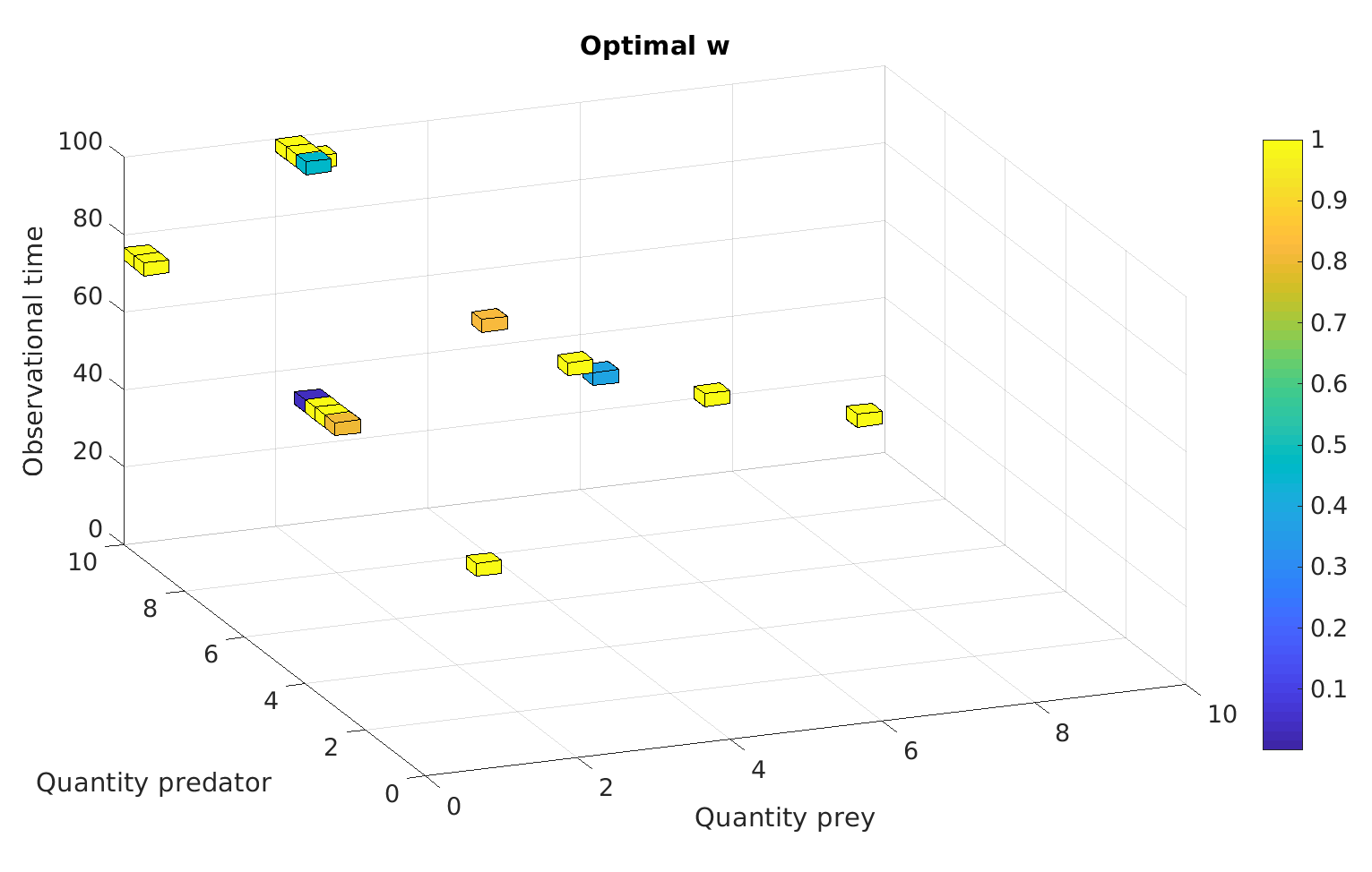
Figure 4.2: Solution of Example 4.1 for the logarithmic D-criterion ($q=0$ in (1.4)) with $\alpha=0$. Entries equal to zero are not shown.

Due to the fact that the cost per iteration for FISTA and PGMA is different, essentially due to different step size selection mechanisms, we utilize the elapsed CPU time as our performance criterion. In each case, the setup time for the precomputation of the FIMs $\Upsilon_{i}$ is identical and it is not included.

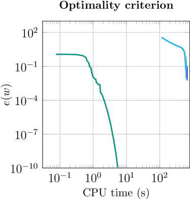
(a)

(b)

Figure 4.3: Example 4.1, comparison of algorithms by (a) value of $e(w)$ from (4.6) and (b) size of the support of $w$.

Fig. 4.3a compares both algorithms for $\alpha=0$ and $\alpha=10^{-6}$ with respect to the decay of the error function (4.6) over CPU time. We clearly observe the PGMA outperforms FISTA by far. The latter was stopped after $5000$ iterations without coming close to the desired tolerance. By contrast, PGMA reached the stopping criterion (4.7) after about 5.6 CPU seconds and within 300 iterations.

A further aspect of comparison of these algorithms is presented in Fig. 4.3b, where the size of the support of the iterates is shown. Again PGMA outperforms FISTA, although the latter reaches an iterate with almost the same degree of sparsity as the optimal solution after almost $5000$ iterations. A partial explanation for the superiority of PGMA is based on the fact that it utilizes larger step sizes, in particular with regard to $\gamma_{k}$; see Fig. 4.4. For FISTA, we observe that $\gamma_{k}$ is quite small and constant. Notice that FISTA does not allow $\gamma_{k}$ to increase, and its size is determined by the initial guess. Furthermore $\theta_{k}$ is chosen a-priori, thus practically there is no adaptivity in the choice of the step sizes in FISTA. PGMA starts from the same initial guess and thus also exhibits small values of $\gamma_{k}$ initially. In constrast to FISTA, however, $\gamma_{k}$ is allowed to increase and does so until a reasonable magnitude is reached. It is then about five orders of magnitude larger than for FISTA. Notice also that $A$ is only locally Lipschitz, which suffices to give theoretical convergence guarantees for PGMA but not for FISTA.

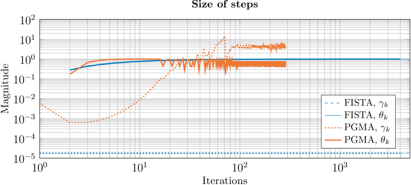
Figure 4.4: Example 4.1 with $\alpha=0$, comparison of algorithms by step sizes $\gamma_{k}$ and $\theta_{k}$.

Returning to Fig. 4.3a, we observe that both algorithms are only affected in a minor way by the choice of the regularization parameter $\alpha$. Apparently, the non-uniqueness of the optimal weight in the case $\alpha=0$ does not represent an obstacle to the convergence.

4.5 Comparison of Different Design Criteria

In this section we compare the convergence behavior of PGMA for solving Example 4.1 with various design criteria, i.e., for different choices of $q$, as well as for various values of the regularization parameter $\alpha$. We chose $\alpha=0$ and $\alpha=10^{-3}$ and five different quantities of $q$ in order to observe different sparsity patterns. All used combinations as well as the resulting size of the support of the solution is presented in Table 4.1. Recall that $q=0$ refers to the logarithmic D-criterion while $q=1$ denotes the A-criterion. Furthermore we approximate the E-criterion by setting $q=10$.

Again the comparison of both Algorithms 2 and 3 is based on CPU time, excluding the setup time for the elementary FIMs $\Upsilon_{i}$.

Table 4.1: Comparison of the size of the support for Fig. 4.1 with different design criteria.

$\alpha$	$q=0$	$q=\frac{1}{2}$	$q=1$	$q=2$	$q=10$
$0$	16	16	15	16	16
$10^{-3}$	16	$27\,000$	$27\,000$	$27\,000$	$27\,000$

The convergence results are presented in Fig. 4.5.

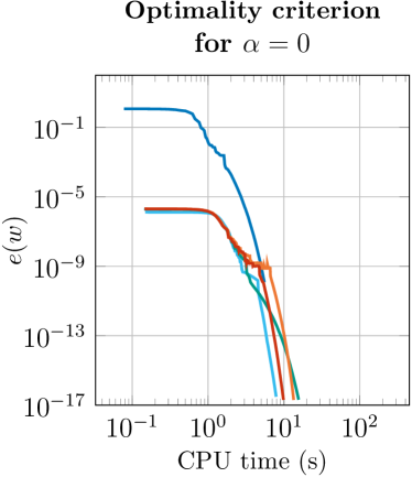
(a)

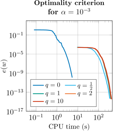
(b)

Figure 4.5: Example 4.1 solved with PGMA. Comparison of design criteria for different choices of $\alpha$ by the value of $e(w)$ from (4.6).

First we observe that in all variants PGMA, reached an iterate which fulfilled the stopping criterion (4.7). Furthermore Figs. 4.5a and 4.5b indicate that in case $q=0$ there are only minor differences in computational time for different values of $\alpha$. Indeed PGMA took $5.8$ respectively $5.1$ seconds to converge for $\alpha=0$ and $\alpha=10^{-3}$. In case $q>0$ the computational time for $\alpha=0$ and $\alpha=10^{-3}$ is about 10 and 400 seconds respectively, almost independently of the particular choice of $q$.

5 Acceleration Strategies

In this section we present four acceleration strategies for the aforementioned algorithms. All of them replace the solution of the discrete problem (3.5) by a sequence of smaller problems of the same or similar type. Consequently, FISTA and PGMA can both serve as inner solvers but based on the findings of the previous section, we focus on PGMA.

The motivation for further acceleration is based on the interest of solving discretized OED problems for large values of $m$ which arise from high dimensional design spaces and/or fine discretization. We exploit the polyhedral structure of the feasible set in (3.5) and utilize that an optimal solution can be represented by a certain linear combination of vertices of $\Delta_{C}\cap\mathcal{B}$ or $\Delta_{C}$.

5.1 Simplicial Decomposition

The first strategy we consider is the well known Simplicial Decomposion (SD) as presented in [29, 42]. This approach utilizes that each point in the polyhedron $\Delta_{C}\cap\mathcal{B}$ can be written as a convex combination of vertices of $\Delta_{C}\cap\mathcal{B}$. We denote these vertices by $s_{i}$, $i=1,\ldots,r$. Consequently, any $w\in\Delta_{C}\cap\mathcal{B}$ can be expressed as

$$w=\sum_{i=1}^{r}\lambda_{i}\,s_{i}\text{ for some }\lambda_{i}\geq 0\text{ satisfying }\sum_{i=1}^{r}\lambda_{i}=1.$$ (5.1)

Note that by straightforward geometric reasoning we obtain

$$r\geq\max\left\{\text{nnz}(w)-\text{neo}(w),1\right\}.$$

Recall that nnz and neo denote the numbers of non-zero entries, and of entries equal to one, respectively; see (3.7).

In a nutshell, the simplicial decomposition algorithm restricts the search for an optimal weight vector in $\Delta_{C}\cap\mathcal{B}$ to the convex hull of a few active vertices of $\Delta_{C}\cap\mathcal{B}$. In each iteration, a new vertex is added to the active set, and unused ones are removed. The vertex added is one which yields the minimal value of the directional derivative of the objective.

The complete simplicial decomposition algorithm is described in Algorithm 4.

Algorithm 4 Simplicial Decomposition (SD)

0:  $\left\{s^{(0),i}\right\}_{i=1}^{r^{(0)}}$ (vertices of $\Delta_{C}\cap\mathcal{B}\subset\mathbb{R}^{m}$) such that $\displaystyle\Lambda\Biggl{(}\sum_{i=1}^{r^{(0)}}s^{(0),i}\Biggr{)}\succ 0$

1:  Set $R^{(0)}\coloneqq\left[s^{(0),1}\cdots\,s^{(0),r^{(0)}}\right]$

2:  Set $w^{(0)}\coloneqq\left(r^{(0)}\right)^{-1}R^{(0)}\mathbf{1}$ and $k\coloneqq 1$ /​/ $w^{(0)}$ is the average of the $s^{(0),i}$

3:  repeat

4:     Compute a vertex $s^{(k)}\in\mathbb{R}^{m}$ which solves the linear program

$$\text{Minimize }s^{\mkern-1.5mu\mathrm{T}}\Lambda^{*}\nabla F_{q}(\Lambda w^{(k)})\quad\text{s.t. }s\in\Delta_{C}\cap\mathcal{B}$$ (OUT_SD)

5:     Set $\bar{R}\coloneqq[R^{(k)},\;s^{(k)}]$

6:     Compute $\lambda^{(k+1)}$ as an inexact solution of the so-called restricted master problem

$$\text{Minimize }F_{q}(\Lambda\bar{R}\lambda)\quad\text{s.t. }\lambda\in\Delta_{1}$$ (IN_SD)

To this end, we use Algorithm 5 with tolerance $\delta$ in (5.7).

7:      Set $\lambda^{(k+1)}_{i}\coloneqq\begin{cases}\lambda^{(k+1)}_{i}&\text{if }\lambda^{(k+1)}_{i}>\sqrt{\delta}/2\\ 0&\text{else }\end{cases}$

8:      Set $\lambda^{(k+1)}=\lVert\lambda^{(k+1)}\rVert_{1}^{-1}\lambda^{(k+1)}$

9:     Set $R^{(k+1)}\coloneqq\bar{R}[\,:\,,(\lambda^{(k+1)}>0)]$ /​/ purge unused vertices

10:     Set $w^{(k+1)}\coloneqq\bar{R}\lambda^{(k+1)}$

11:     if the inital guess of $\lambda$ in (IN_SD) fulfills (5.7) in Algorithm 5 with tolerance $\delta$ then

12:        Set $\delta\coloneqq\delta/10$

13:     end if

14:     Set $k\coloneqq k+1$

15:  until stopping criterion (4.7) is fulfilled

It is important to point out that we restrict our tests to cases $q\in[0,1]$ and $\alpha=0$, thus in particular only problems without regularization. This apporach is based on the fact that we do not provide algorithms for the solution of the inner problem (IN_SD) in more general cases.

The initial values $\left\{s^{(0),i}\right\}_{i=1}^{r^{(0)}}$ for Algorithm 4 are determined in the following way. We first solve (OUT_SD) with $\Lambda^{*}\nabla F_{q}(\Lambda w)$ where $w$ is a feasible vector with all entries equal. This yields in $s^{(0),1}$. If $\Lambda s^{(0),1}\succ 0$ does not hold, we iteratively insert further vertices of $\Delta_{C}\cap\mathcal{B}$ randomly until this condition is fulfilled for the sum of all considered vertices.

Next we discuss how the subproblems (OUT_SD) and (IN_SD) can be solved.

The linear program (OUT_SD) can be solved explicitly by sorting the entries of $\Lambda^{*}\nabla F_{q}(\Lambda w^{(k)})$ and assigning the entries equal to one and potentially entries in $(0,1)$ in $s^{(k)}$ in a greedy fashion. In case several entries of $\Lambda^{*}\nabla F_{q}(\Lambda w^{(k)})$ agree, we make sure that the corresponding entries of $s^{(k)}$ agree as well.

Concerning the restricted master problem (IN_SD), notice that this problem varies in dimension from iteration to iteration, depending on the number of active vertices, i.e., columns of $\bar{R}$. For the subsequent discussion we omit the iteration index and denote this dimension by $r$. In order to compare (IN_SD) with the settings as in Section 3, we introduce the FIM associated with the $j$-th vertex in the set of active vertices $\bar{R}$ as

$$\bar{\Upsilon}_{j}\coloneqq\sum_{i=1}^{m}\Upsilon_{i}\lvert E_{i}\rvert\bar{R}_{i,j}=\Lambda\bar{R}[\,:\,,j].$$ (5.2)

It is worth noting that $\bar{\Upsilon}_{j}$ is symmetric and positive semi-definite since $\Upsilon_{i}$ has this property and the entries in $\bar{R}$, consisting of vertex coordinates of $\Delta_{C}\cap\mathcal{B}$, are non-negative. Next we represent the synthesis operator (3.1) in terms of the barycentric coordinates $\lambda\in\mathbb{R}^{r}$:

$$\bar{\Lambda}\lambda\coloneqq\Lambda\bar{R}\lambda=\sum_{j=1}^{r}\lambda_{j}\,\bar{\Upsilon}_{j}.$$ (5.3)

The weight constraint is expressed as

$$C=\mathbf{1}^{\mkern-1.5mu\mathrm{T}}Mw=\mathbf{1}^{\mkern-1.5mu\mathrm{T}}M\bar{R}\lambda=\sum_{i=1}^{m}\lvert E_{i}\rvert\sum_{j=1}^{r}\bar{R}_{i,j}\lambda_{j}=\sum_{j=1}^{r}\lambda_{j}\sum_{i=1}^{m}\lvert E_{i}\rvert\bar{R}_{i,j}=C\sum_{j=1}^{r}\lambda_{j}$$ (5.4)

and thus it reduces to $\mathbf{1}^{\mkern-1.5mu\mathrm{T}}\lambda=1$. To summarize, (IN_SD) can be written as

Minimize $$F_{q}(\bar{\Lambda}\lambda),\quad\lambda\in\mathbb{R}^{r}$$ (5.5)

s.t. $$\lambda\geq 0$$

and $$\mathbf{1}^{\mkern-1.5mu\mathrm{T}}\lambda=1.$$

Notice that, in contrast to (3.5), (5.5) does not feature pointwise upper bounds on the variable $\lambda$.

Unfortunately, the first-order methods discussed in Section 4 are not efficiently applicable for the solution of the resctriced problems (5.5). The reason is that both Algorithm 2 (FISTA) and Algorithm 3 (PGMA) require the orthogonal projection onto $\Delta_{C}\cap\mathcal{B}$. In (5.5), the appropriate inner product is given by

$$\left(\bar{R}\lambda_{1},\bar{R}\lambda_{2}\right)_{M}=\lambda_{1}^{\mkern-1.5mu\mathrm{T}}\bar{R}^{\mkern-1.5mu\mathrm{T}}M\bar{R}\lambda_{2}=\lambda_{1}^{\mkern-1.5mu\mathrm{T}}\bar{M}\lambda_{2}$$ (5.6)

with $\bar{M}\coloneqq\bar{R}^{\mkern-1.5mu\mathrm{T}}M\bar{R}$. In contrast to $M$, the reduced inner product matrix $\bar{M}$ is, in general, not diagonal. Therefore, the evaluation of the projection cannot be achieved as in Algorithm 1 but it becomes significantly more expensive. In addition, $\bar{M}$ is, in general, only positive semi-definite.

In order to present numerical results for Algorithm 4, we resort to a simple solver for the inner problem (5.5). As mentioned in the introduction, an approach described in the literature is Torsney’s multiplicative algorithm; see Algorithm 5. It was described and analyzed in [37, 39, 46] and specifically in [41, 17] in the context of simplicial decomposition. We point out that Algorithm 5 is only applicable when $\alpha=0$, i.e., for the unregularized problem, and for $q\in[0,1]$ (cf. [46]).

Algorithm 5 Torsney’s algorithm for (IN_SD) ($\alpha=0$ and $q\in[0,1]$)

0:  $\lambda^{[0]}\in\mathbb{R}^{r}$

1:  Set $j\coloneqq 0$

2:  repeat

3:     Set

$$\lambda^{[j+1]}_{i}\coloneqq\lambda^{[j]}_{i}\frac{\nabla F_{q}(\bar{\Lambda}\lambda^{[j]})\dprod\bar{\Upsilon}_{i}}{\nabla F_{q}(\bar{\Lambda}\lambda^{[j]})\dprod\bar{\Lambda}\lambda^{[j]}},\quad i=1,\ldots,r$$

4:     Set $j\coloneqq j+1$

5:  until $\lambda^{[j]}$ fulfills the stopping criterion (5.7)

Algorithm 5 is very easy to implement. Notice that we denote the iteration counter $\cdot^{[j]}$ with square brackets to avoid a confusion with the outer iteration index $\cdot^{(k)}$ in Algorithm 4. Due to the multiplicative nature of Algorithm 5 we have to initialize it with $\lambda^{[0]}$ strictly positive. In the very first call to Algorithm 5, we initialize $\lambda^{[0]}$ as a multiple of an all-ones vector. In subsequent calls to Algorithm 5, we utilize the final iterate of the previous call to create a more informed initial guess. To be precise, we remove unused coordinates, initialize the new coordinate with $1/r$ and rescale the remaining entries so that the total sum equals one.

We stop Algorithm 5 as soon as

$$\lambda_{i}^{[j]}\,\bigl{(}\max_{k=1,\ldots,r}\nabla F_{q}(\bar{\Lambda}\lambda^{[j]})\dprod\bar{\Upsilon}_{k}-\nabla F_{q}(\bar{\Lambda}\lambda^{[j]})\dprod\bar{\Upsilon}_{i}\bigr{)}\leq\delta$$ (5.7)

holds (cf. also Fig. 5.1) or a maximal number of iterations is reached.

Figure 5.1: Illustration of the stopping criterion (5.7). All pairs $\left(\lambda_{i}^{[j]},\nabla F_{q}(\bar{\Lambda}\lambda^{[j]})\dprod\bar{\Upsilon}_{i}\right)$ must lie in the light gray area or on the bold lines, $i=1,\ldots,r$.

We conclude the description of the simplicial decompositon Algorithm 4, combined with Algorithm 5 as inner solver, by noting that it requires a rounding strategy; see 7 and 8 in Algorithm 4. We first set all entries of $\lambda^{[j]}$ which are less then $\sqrt{\delta}/2$ to zero and later rescale the remaining ones such that all entries of the resulting vector sum up to 1. Therefore we can only expect to obtain inexact solutions of (3.5). Furthermore we observe that due to the non-uniqueness of the solutions of (IN_SD), purging vertices in Algorithm 4 does not necessarily reduce the subproblem to its minimal size.

In spite of these obstacles, we included the classical simplicial decomposition Algorithm 4 for comparison with more efficient accelerated solvers described in the following subsection.

5.2 Methods Based on Active Set Strategies

In this subsection we consider three further acceleration strategies which are based on a common framework given in Algorithm 6. We term this framework the generic active set strategy (GASS). In comparison with the simplicial decomposition (SD) Algorithm 4, the inner problems to be solved in each iteration are different. The three variants of GASS we consider are termed the simplicial decomposition modified (SDM), simplicial decomposition modified with heuristics (SDMH), and primal-dual semiactive set strategy (PDSAS).

To simplify the notation we define $\Delta^{\text{free}}_{C}\coloneqq\{w\in\mathbb{R}^{m}\,|\,(1\,,\,w)_{M}=C\}$. Furthermore we have $\mathcal{B}^{-}\coloneqq\{w\in\mathbb{R}^{m}\,|\,w\geq 0\}$ and $\mathcal{B}^{+}\coloneqq\{w\in\mathbb{R}^{m}\,|\,w\leq 1\}$ and thus $\mathcal{B}=\mathcal{B}^{-}\cap\mathcal{B}^{+}$. The main difference is that this algorithm represents its iterates $w^{(k)}$ as bound constrained convex combinations of vertices of $\Delta_{1}=\Delta^{\text{free}}_{1}\cap\mathcal{B}^{-}$, rather than arbitrary convex combinations of vertices of $\Delta^{\text{free}}_{C}\cap\mathcal{B}$. In other words, any $w$ in $\Delta^{\text{free}}_{C}\cap\mathcal{B}$ can be written as

$$w=\sum_{i=1}^{r}\lambda_{i}\,s_{i}\text{ for some }0\leq\lambda_{i}\leq 1\text{ satisfying }\sum_{i=1}^{r}\lvert E_{i}\rvert\,\lambda_{i}=C,$$ (5.8)

where $s_{i}$, $i=1,\ldots,r$ are vertices of $\Delta_{1}$. The idea of applying this decomposition is based on previous work by [35] (cf. also [19]) and [23]. Notice that the representation (5.8) requires $r\geq\text{nnz}(w)$, which is clearly larger than in (5.1), which was used in Algorithm 4.

In order to better understand the combinatorial effort for solving (3.5), we have to compare the number of vertices in $\Delta^{\text{free}}_{C}\cap\mathcal{B}$ and in $\Delta_{1}$. The latter is clearly equal to $m$. We do not attempt to specify the exact number of vertices for $\Delta^{\text{free}}_{C}\cap\mathcal{B}$ here. However, in the special case $\lvert E_{i}\rvert\equiv\lvert E\rvert$ for all $i=1,\ldots,m$ and $C/\lvert E\rvert$ is integer, then there are precisely

$$\binom{m}{C/\lvert E\rvert}$$

vertices in $\Delta_{C}\cap\mathcal{B}$, which is generally much larger than $m$.

The generic active set strategy in Algorithm 6 utilizes the representation (5.8). The general idea is to split the constraints describing the feasible set $\mathcal{B}$ w.r.t. the bound constraints into two parts. We thus obtain two sets $\mathcal{B}_{\text{inner}}$ and $\mathcal{B}_{\text{outer}}$ satisfying $\mathcal{B}=\mathcal{B}_{\text{inner}}\cap\mathcal{B}_{\text{outer}}$.

By replacing the representation (5.1) with (5.8) we have to identify a larger number of active vertices out of a much smaller set of admissible vertices. As a consequence, we expect Algorithm 6 to perform better in terms of the number of outer iterations, at the mild expense of having bound constraints in the inner problem.

In this subsection we say that a vertex of $\Delta_{1}$ is active if the corresponding entry of $w$ is active regarding the lower bounds, e.g. the entry is equal zero. Note that this is different from the simplicial decomposition approach discussed in Section 5.1, where active vertices corresponded to one ore more entries of $w$ being positive.

Algorithm 6 Generic Active Set Strategy (GASS)

0:  $w^{(0)}\in\Delta_{C}\cap\mathcal{B}$ such that $\Lambda w^{(0)}\succ 0$

0:  splitting of the feasible set w.r.t. the pointwise bound constraints $\mathcal{B}_{\text{inner}}\cap\mathcal{B}_{\text{outer}}=\mathcal{B}$

1:  Set $k=0$

2:  Set $\mathcal{A}^{(0)}=\{1\leq i\leq m\,|\,w_{i}=0\}$

3:  repeat

4:     Outer problem:

$$\text{ Find the set of active vertices }\mathcal{A}^{(k+1)}$$ (OUT_GASS)

5:     Inner problem: Compute $w^{(k+1)}$ as an approximate solution of

Minimize $$F_{q}\left(\Lambda w\right)+\frac{\alpha}{2}\lVert w\rVert_{M}^{2},\quad w\in\Delta^{\text{free}}_{C}\cap\mathcal{B}_{\text{inner}}$$ (IN_GASS)

s.t. $$w_{i}=0\quad\text{ for all }i\in\mathcal{A}^{(k+1)}$$

6:     Set $k\coloneqq k+1$

7:  until $w^{(k)}\in\mathcal{B}_{\text{outer}}$ and stopping criterion (4.7) is fulfilled

The numerical effort of solving Algorithm 6 mainly depends on the splitting of the upper and lower bound constraint set $\mathcal{B}$ into $\mathcal{B}_{\text{inner}}$ and $\mathcal{B}_{\text{outer}}$. Based on that, different strategies to determine $\mathcal{A}^{(k+1)}$ in (OUT_GASS) as well as for solving (IN_GASS) arise. In Table 5.1 we give an overview over the approaches we consider.

Algorithm	$\mathcal{B}_{\text{outer}}$	$\mathcal{B}_{\text{inner}}$	approach for	algorithm for
			(OUT_GASS)	(IN_GASS)
SDM	$\mathbb{R}^{m}$	$\mathcal{B}$	Algorithm 7	Algorithm 3
SDMH	$\mathbb{R}^{m}$	$\mathcal{B}$	Algorithm 8	Algorithm 3
PDSAS	$\mathcal{B}^{-}$	$\mathcal{B}^{+}$	Algorithm 9	Algorithm 3

Table 5.1: Overview of active set algorithms (variants of Algorithm 6).

First we discuss the algorithms SDM and SDMH utilizing the strategy for the active sets described in Algorithm 7 as well as Algorithm 8. Both algorithms are a straightforward modification of the classical SD Algorithm 4, considering that $w$ is a particular linear combination of vertices of $\Delta_{1}$. SDM and SDMH differ in terms of the number of vertices inserted in each iteration, i.e., how much $\lvert\mathcal{A}^{(k+1)}\rvert$ can shrink compared to $\lvert\mathcal{A}^{(k)}\rvert$ in (OUT_GASS). While SDM frees exactly one vertex, SDMH frees all local minimizers of the gradient. Therefore we expect that the size of the inner problems in SDM will be smaller, possibly at the expense of an increased number of outer iterations.

Algorithm 7 Approach for (OUT_GASS) in SDM

0:  previous active set $\mathcal{A}^{(k)}$ and previous $w^{(k)}$

1:  Compute $s^{(k)}\in\left\{1,\dots,m\right\}$ which fulfills

$$s^{(k)}=\operatorname*{arg\,min}\left\{\left(\Lambda^{*}\nabla F_{q}(\Lambda w^{(k)})\right)_{i}+\alpha\,w^{(k)}_{i}\,\middle|\,i\in\mathcal{A}^{(k)}\right\}$$

2:  Set $\mathcal{A}^{(k+1)}\coloneqq\left\{i\in\left\{1,\dots,m\right\}\,\middle|\,w_{i}^{(k)}=0\right\}\setminus\left\{s^{(k)}\right\}$

Algorithm 8 Approach for (OUT_GASS) in SDMH

0:  previous active set $\mathcal{A}^{(k)}$ and previous $w^{(k)}$

1:  Compute $S^{(k)}\subset\mathcal{A}^{(k)}$ as the set of all indicies corresponding to local minimizers (with respect to $X$) of the mapping

$$\mathcal{A}^{(k)}\ni i\mapsto\left(\Lambda^{*}\nabla F_{q}(\Lambda w^{(k)})\right)_{i}+\alpha\,w^{(k)}_{i}\in\mathbb{R}.$$

2:  Set $\mathcal{A}^{(k+1)}\coloneqq\left\{i\in\left\{1,\dots,m\right\}\,\middle|\,w_{i}^{(k)}=0\right\}\setminus S^{(k)}$

The solution of problem (IN_GASS) by Algorithm 3 benefits from a good initial guess. When $k=0$, we use a constant vector on the active coordinates. In subsequent iterations of Algorithm 6, we make use of the previous solution $w^{(k)}$ with unused coordinates removed and new entries initialized to $0$.

The third algorithm we consider is a primal-dual semiactive set strategy (PDSAS). Its name derives from the fact that a primal-dual active set approach similarly to [5, 18] is applied, but solely w.r.t. the lower bound constraints $\mathcal{B}^{-}$. The reason to leave the upper bound constraints to (IN_GASS) is that otherwise, the active constraints may become incompatible with the mass constraint $w\in\Delta^{\text{free}}_{C}$.

As the name indicates we will make use of the dual variables of (IN_GASS). In order to motivate these dual variables we recall (3.5):

Minimize $$F_{q}(\Lambda w)+\frac{\alpha}{2}\lVert w\rVert_{M}^{2},\quad w\in\mathbb{R}^{m}$$

s.t. $$0\leq w\leq 1$$

and $$\mathbf{1}^{\mkern-1.5mu\mathrm{T}}Mw=C.$$

Next we indroduce the dual variables $\mu^{-}\in\mathbb{R}^{m}$ for the lower and $\mu^{+}\in\mathbb{R}^{m}$ for the upper bounds as well as $\zeta\in\mathbb{R}$ for the weight constraint. The corresponding KKT conditions can be formulated as

$$0 =\Lambda^{*}\nabla F\left(\Lambda w\right)+\alpha\,w-\mu^{-}+\mu^{+}+\zeta\mathbf{1}$$

$$0 \leq w\,\perp\,\mu^{-}\geq 0$$

$$0 \leq 1-w\perp\,\mu^{+}\geq 0$$

since $M$ is spd and diagonal. By applying the complementarity function $\mathbb{R}^{2}\ni(a,b)\mapsto\max\left\{a,cb\right\}\in\mathbb{R}$ for arbitrary $c>0$ and replacing $\mu^{-}$ by $\nu\coloneqq-\mu^{-}$, this system is seen to be equivalent to

$$\mu^{+} =\max\left\{-\Lambda^{*}\nabla F\left(\Lambda w\right)-\alpha\,w-\zeta\mathbf{1},\;0\right\}$$ (5.9a)

$$\nu =\min\left\{-\Lambda^{*}\nabla F\left(\Lambda w\right)-\alpha\,w-\zeta\mathbf{1},\;0\right\}$$ (5.9b)

$$0 =\nu-\min\left\{0,c\,w+\nu\right\}$$ (5.9c)

$$0 \leq 1-w\,\perp\,\mu^{+}\geq 0.$$ (5.9d)

In contrast to SDM and SDMH, we make use of the dual variables $\nu$ and $\zeta$ in order to estimate the active set $\mathcal{A}\coloneqq\{1\leq i\leq m\,|\,w_{i}=0\}$ in each iteration. Algorithmically this can be done by computing $\nu^{(k)}$ via (5.9b) with $w^{(k)}$ as the solution of the previous inner problem and $\zeta^{(k)}$ the corresponding multiplier of the weight constraint. Next by (5.9c) we clearly have

$$c\,w^{(k)}+\nu<0\quad\Rightarrow\quad\nu>0\quad\Rightarrow\quad w=0$$

what will be used to compute $\mathcal{A}^{(k+1)}$. Furthermore we also have to consider the case that for given $w^{(k)}$, $\nu^{(k)}$ as well as $c$, the set $\mathcal{A}^{(k+1)}$ is so large that

$$C\leq\sum_{\mathchoice{\makebox[0.0pt][l]{$\displaystyle\vphantom{}{i\notin\mathcal{A}^{(k+1)}}$}}{\makebox[0.0pt][l]{$\textstyle\vphantom{}{i\notin\mathcal{A}^{(k+1)}}$}}{\makebox[0.0pt][l]{$\scriptstyle\vphantom{}{i\notin\mathcal{A}^{(k+1)}}$}}{\makebox[0.0pt][l]{$\scriptscriptstyle\vphantom{}{i\notin\mathcal{A}^{(k+1)}}$}}}\lvert E_{i}\rvert$$ (5.10)

is violated. In this case, the inner problem (IN_GASS) is not feasible. It turns out that by increasing $c$ in these cases we can ensure the feasibility of the inner problem.

The described approach is summarized in Algorithm 9. As initial guess for (IN_GASS) we use the constant feasible vector in each iteration of Algorithm 6.

Algorithm 9 Approach for (OUT_GASS) in PDSAS

0:  previous $w^{(k)}$, $\zeta^{(k)}$, parameter $c$

0:  $\mathcal{A}^{(k+1)}$ and $c>0$

1:  Set $\nu^{(k)}\coloneqq\min\left\{-\Lambda^{*}\nabla F_{q}(\Lambda w^{(k)})-\alpha\,w^{(k)}-\zeta^{(k)},\;0\right\}$

2:  repeat

3:     Set $\mathcal{A}^{(k+1)}\coloneqq\bigl{\{}1\leq i\leq m\,\big{|}\,\nu^{(k)}_{i}+c\ w^{(k)}_{i}<0\bigr{\}}$

4:     if (5.10) is violated then

5:        Set $c\coloneqq 10c$

6:     end if

7:  until (5.10) is fulfilled

5.3 Comparison of Accelerated Algorithms 1

In this section we compare the accelerated algorithms presented in Table 5.1 as well as PGMA. Again we make use of Example 4.1, considering $\alpha=0$ as well as $q=0$, i.e., the logarithmic D-criterion. We refine the discretization of $X$ to contain $50^{3}=$125\,000$$ $\mathcal{DG}_{0}$-elements. Besides the regular stopping criterion we stopped the algorithms from Table 5.1 after $300$ iterations when necessary. For the solution of each restricted master problem, see 6 of Algorithm 4, we allowed up to $5\cdot 10^{4}$ iterations of Torsney’s Algorithm 5. The same iteration limit is used for Algorithm 3 for the solution of (IN_GASS). The results are described in Fig. 5.2. As before, the time to setup the elementary Fisher information matrices is excluded from all timings.

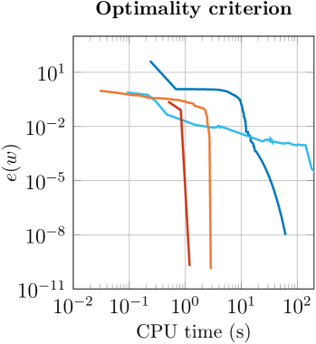
(a)

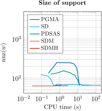
(b)

Figure 5.2: Example 4.1 with $m=$125\,000$$; comparison of accelerated algorithms for $\alpha=0$ by (a) value of $e(w)$ from (4.6) and (b) size of the support.

First we compare the violation of the contraints versus the CPU time elapsed. The corresponding chart can be found in Fig. 5.2a. All algorithms beside SD reached an iterate which fulfills the stopping criterion (4.7). Note that all iterates of PDSAS exept the last one are infeasible. (Due to numerical errors this is also the case of some iterates of SD.) Therefore PDSAS is omitted from Fig. 5.2a. While PDSAS needed 13.7 seconds, SDM took about 2.8 seconds and SDMH took less than 1.5 seconds to terminate. For comparison, the unaccelerated PGMA (Algorithm 3) required 62 seconds to run.

Next in Fig. 5.2b we compare the number of non-zero elements of the iterates. Obviously the usage of PGMA results in iterates with the largest sizes of support. The first iterates of SD also have a large support, what can be explained by the fact that each used vertex increases the size of the support possibly by more than one. Considering PDSAS we plotted the quantity of positive entries of the iterates. Nevertheless due to the construction of the algorithm every iterate execpt the final one contains negative entries. Such a behavior is not observed by SDM or SDMH since here the inserted vertices have only one non-zero element each. Thus the size of the support of the iterates does not grow larger than the support of the solution. All algorithms reached an iterate with 65 non-zero elements. Nevertheless one should keep in mind that the results of SD are rounded while the others are not.

Let us finally compare the behavior of the algorithms in more detail. While it took less than 0.1 seconds to compute the first iterate in SD and SDM, SDMH required about 0.8 seconds. But already the third iterate of SDMH (after 1.5 seconds) fulfilled the stopping criterion (4.7), whereas the other algorithms needed much more time to terminate. This behavior confirms our expectations described in Section 5.2, that SDMH might require fewer outer iterations but generally has larger inner problems than SDM.

5.4 Comparison of Accelerated Algorithms 2

In this subsection, we consider only the two best algorithms from Section 5.3, SDM and SDMH. The example is taken from [26] and it is even larger than our previous examples.

Example 5.1 (Stationary diffusion problem).

We consider the nonlinear model

$$-\nabla\cdot\bigl{(}\exp(m_{p})\nabla y\bigr{)} =0 \text{in }\Omega\coloneqq(0,1)^{2}$$

$$y =x_{1} \text{on }\Gamma_{D}\coloneqq\{0,1\}\times(0,1)$$

$$\exp(m_{p})\,\partial_{n}y =0 \text{on }\partial\Omega\setminus\Gamma_{D},$$

where $m_{p}(x)=\sum_{i=1}^{5}\sum_{j=1}^{5}p(i,j)\sin(\pi ix_{1})\sin(\pi jx_{2})$.

Since this is a sensor placement problem, the design space $X$ equals the domain $\Omega$. The sensitivity of $y$ w.r.t $p(i,j)$ will be denoted by $\delta y_{i,j}$ and fulfills $-\nabla\cdot\left(\exp(m_{q})\cdot\nabla\delta y_{i,j}\right)=\nabla\cdot\left(\exp(m_{q})\sin(i\pi x_{1})\sin(j\pi x_{2})\nabla y\right)$ in $\Omega$ together with the boundary conditions $\delta y_{i,j}=$ on $\Gamma_{D}$ and $\exp(m_{q})\partial_{n}\delta y_{i,j}=0$ on $\partial\Omega\setminus\Gamma_{D}$. Arranging the full set of sensitivities into the matrix

$$\delta y=\begin{pmatrix}\delta y_{1,1}&\dots&\delta y_{1,5}\\ \vdots&&\vdots\\ \delta y_{5,1}&\dots&\delta y_{5,5}\end{pmatrix}$$

we find the following expression for the elementary Fisher information matrices:

$$\Upsilon(x)=\operatorname{vec}(\delta y(x))^{\mkern-1.5mu\mathrm{T}}\operatorname{vec}(\delta y(x))\in\mathbb{R}^{25\times 25}.$$

Recall that we take $\Upsilon_{i}$ on each cell of the discretized design space $X$ to be its value in the midpoint. We choose $p=0\in\mathbb{R}^{5\times 5}\simeq\mathbb{R}^{25}$ as nominal value of the parameter. We discretize $\Omega$ as well as $X$ by identical meshes containing $m\approx$430\,000$$ triangular elements. Each element has maximal edge length of $0.0057$ but the elements are not precisely of equal size. We set $C=10^{-4}\lvert X\rvert=10^{-4}$, so the experimental budget allows us to allocate a total weight of $0.01\%$ of the sum of the weights of all admissible experiments.

We aim to solve Example 5.1 for $\alpha=0$ and $q=0$, i.e., we consider the logarithmic D-criterion for the unregularized problem. The preprocessing of the data $\Upsilon_{i}$ (which is once again not included in the timings) takes about $610$ CPU seconds. Based on the observations in Section 5.3 we only present the results for SDM and SDMH (see Table 5.1), since the remaining methods exhibit a much slower convergence behavior. Similarly as in the previous example, besides the stopping criteria already decribed, the algorithm for solving the inner problems (IN_GASS) also terminates when $10^{4}$ iterations are reached.

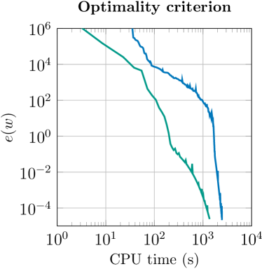
(a)

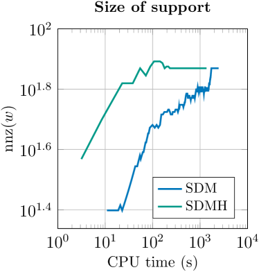
(b)

Figure 5.3: Example 5.1 for $\alpha=0$ and $q=0$, Comparison of accelerated algorithms with PGMA as algorithm for the RMP’s by (a) value of $e(w)$ from (4.6) and (b) size of the support out of a maximum of $m\approx$430\,000$$.

Figure 5.3a compares the satisfaction of the optimality criterion as measured by (4.6). The algorithms SDM and SDMH needed $2400$ and $1300$ CPU seconds, respectively. Figure 5.3b describes the support of the iterates over the time. Similarily as in the previous example, SDM and SDMH typically underestimate the size of the support until convergence.

6 Discussion

In this paper we discussed first-order methods (FISTA and PGMA) for a class of optimal experimental design (OED) problems, which contain pointwise upper bounds as well as a maximal total weight. PGMA exhibited a significanly more favorable convergence behavior, which can be explained by the fact that FISTA is unable to increase the stepsize $\gamma_{k}$. It turns out that this strategy is not ideal for the problem class under consideration.

Subsequently, we discussed four acceleration strategies. These comprised the simplicial decomposition method (Algorithm 4) with Torsney’s Algorithm 5 as inner solver, as well as three variants (SDM, SDMH, PDSAS) of a generic active set strategy (GASS). The latter are based on the idea of working with vertices of the simplex $\Delta_{C}$ rather than vertices of polyhedron $\Delta_{C}\cap\mathcal{B}$ . As was illustrated in Fig. 5.2, the methods of class GASS outperform PGMA as well as SD.

The algorithms of class GASS differ w.r.t. the strategy of how many entries of $w^{(k)}$ may become inactive in one iteration. While SDM allows this only for one entry per iteration, SDMH allows several. As expected, allowing more entries to become active may decrease the number of outer iterations at the cost of an increasing size of the inner problems. For the examples considered throughout this paper, SDMH outperformed SDM, but we make no claim that this is always the case. We also considered a version of the primal-dual active set strategy, which we termed PDSAS. In our experiments, this strategy was not as effective SDM or SDMH but still outperformed simplicial decomposition with Torsney’s method as inner solver.

The precomputation of the elementary Fisher information matrices $\Upsilon_{i}$ is a significant part of the overall run time for large scale problems. Therefore, there is opportunity to develop adaptive discretization strategies of the design space to further reduce computational cost.

Appendix A Proof of Lemma 3.4

Proof A.1.

Part $(a)$: Recall the definitions $W(v)\coloneqq\sum_{i=1}^{m}\lvert E_{i}\rvert v_{i}$ and $P(\zeta)\coloneqq\operatorname{proj}_{\mathcal{B}}(f-\zeta)$ from (3.7), where $\mathcal{B}=[0,1]^{m}$. For arbitrary numbers $\zeta_{1}>\zeta_{2}$ we get

$$W(P(\zeta_{1}))-W(P(\zeta_{2}))=W(P(\zeta_{1})-P(\zeta_{2}))\leq 0$$

since $P(\zeta_{1})\leq P(\zeta_{2})$ and $\lvert E_{i}\rvert>0$ holds for all $i=1,\dots,m$.

Equation 3.10: We split the proof into two cases. Recall that the function $\zeta$ was defined in (3.9) and that we assumed that the entries in $f$ are sorted in descending order. First we handle the case $\ell^{*}=k^{*}$, where obviously $\sum_{i=1}^{k^{*}}\lvert E_{i}\rvert=C$ holds. By a simple reformulation we get

$${2}\zeta(k^{*},k^{*}-1) =\lvert E_{k^{*}}\rvert^{-1}\left(\sum_{i=1}^{k^{*}-1}\lvert E_{i}\rvert+\lvert E_{k^{*}}\rvert f_{k^{*}}-C\right)$$

$$=f_{k^{*}}+\lvert E_{k^{*}}\rvert^{-1}\left(\sum_{i=1}^{k^{*}-1}\lvert E_{i}\rvert-C\right)$$

$$=f_{k^{*}}+\lvert E_{k^{*}}\rvert^{-1}(-\lvert E_{k^{*}}\rvert)$$

$$=f_{k^{*}}-1$$

$$=\zeta(k^{*},k^{*}).$$

In the second case, i.e., $0\leq\ell\leq k^{*}-2$, we have from (3.9)

$$\left(\sum_{i=\ell+1}^{k^{*}}\lvert E_{i}\rvert\right)\,\zeta(k^{*},\ell) =\sum_{i=1}^{\ell}\lvert E_{i}\rvert+\sum_{i=\ell+1}^{k^{*}}\lvert E_{i}\rvert f_{i}-C$$

$$=\sum_{i=1}^{\ell+1}\lvert E_{i}\rvert+\sum_{i=\ell+2}^{k^{*}}\lvert E_{i}\rvert f_{i}-C-\lvert E_{\ell+1}\rvert+\lvert E_{\ell+1}\rvert f_{\ell+1}$$

$$=\left(\sum_{i=\ell+2}^{k^{*}}\lvert E_{i}\rvert\right)\,\zeta(k^{*},\ell+1)+\lvert E_{\ell+1}\rvert(f_{\ell+1}-1).$$

By further reformulation we get

$$\left(\sum_{i=\ell+1}^{k^{*}}\lvert E_{i}\rvert\right)\,\zeta(k^{*},\ell) =\left(\sum_{i=\ell+2}^{k^{*}}\lvert E_{i}\rvert\right)\,\zeta(k^{*},\ell+1)+\lvert E_{\ell+1}\rvert(f_{\ell+1}-1)$$

$$\Leftrightarrow\quad \lvert E_{\ell+1}\rvert\,\zeta(k^{*},\ell)+\left(\sum_{i=\ell+2}^{k^{*}}\lvert E_{i}\rvert\right)\,\zeta(k^{*},\ell) =\left(\sum_{i=\ell+2}^{k^{*}}\lvert E_{i}\rvert\right)\,\zeta(k^{*},\ell+1)+\lvert E_{\ell+1}\rvert(f_{\ell+1}-1)$$

$$\Leftrightarrow\quad \lvert E_{\ell+1}\rvert(\zeta(k^{*},\ell)-f_{\ell+1}+1) =\left(\sum_{i=\ell+2}^{k^{*}}\lvert E_{i}\rvert\right)\,\bigl{(}\zeta(k^{*},\ell+1)-\zeta(k^{*},\ell)\bigr{)}.$$

Since $\lvert E_{i}\rvert>0$ holds for all $i$, we obtain (3.10).

Part $(c)$: Note that due to $k^{*}=\ell^{*}$ and assumption (1.10) we have $k^{*}=\ell^{*}<m$. First we prove the statment for $i=k^{*}$:

$$f_{k^{*}+1}-\zeta(k^{*},k^{*})=f_{k^{*}+1}-(f_{k^{*}}-1)<1,$$

where we used the definition of $\zeta$ in (3.9) and the fact that $f_{k^{*}+1}$ is stricly less than $f_{k^{*}}$ since the entries of $f$ are sorted and $v_{k^{*}+1}=\operatorname{proj}_{[0,1]}(f_{k^{*}+1}-\zeta^{*})=0<v_{k^{*}}$.

Now we consider $i\in\{1,\dots,k^{*}-1\}$. Note since $k^{*}=\ell^{*}$ we have $\sum_{i=1}^{k^{*}}\lvert E_{i}\rvert=C$ and thus

$$f_{i+1}-\zeta(k^{*},i) =f_{i+1}-\left(\sum_{j=i+1}^{k^{*}}\lvert E_{j}\rvert\right)^{-1}\left(\sum_{j=1}^{i}\lvert E_{j}\rvert+\sum_{j=i+1}^{k^{*}}\lvert E_{j}\rvert f_{j}-C\right)$$

$$=f_{i+1}-\left(\sum_{j=i+1}^{k^{*}}\lvert E_{j}\rvert\right)^{-1}\left(-\sum_{j=i+1}^{k^{*}}\lvert E_{j}\rvert+\sum_{j=i+1}^{k^{*}}\lvert E_{j}\rvert f_{j}\right)$$

$$=f_{i+1}-\left(\sum_{j=i+1}^{k^{*}}\lvert E_{j}\rvert\right)^{-1}\left(\sum_{j=i+1}^{k^{*}}\lvert E_{j}\rvert(f_{j}-1)\right)$$

$$\geq f_{i+1}-\left(\sum_{j=i+1}^{k^{*}}\lvert E_{j}\rvert\right)^{-1}\left(\sum_{j=i+1}^{k^{*}}\lvert E_{j}\rvert\right)(f_{i+1}-1)$$

$$=1.$$

This estimate is based on the fact that $f_{j}\leq f_{i+1}$ holds for all $j\geq i+1$.

Part $(d)$: First we observe that if $f_{j+1}-\zeta(k^{*},j)<1$ holds for some $j\in\{\ell_{\min},\dots,k^{*}-1\}$, then this is also the case for all $i\in\{j+1,\dots,k^{*}-1\}$. This can be proved iteratively since for $j\leq k^{*}-2$ one gets

$$1>f_{j+1}-\zeta(k^{*},j)\geq f_{j+2}-\zeta(k^{*},j)>f_{j+2}-\zeta(k^{*},j+1)$$ (A.1)

by utilizing (3.10).

Now the following strategy is applied iteratively for increasing $i\in\{\ell_{\min},\dots,k^{*}-1\}$. If $1\leq f_{i+1}-\zeta(k^{*},i)$ holds, we can increase $i$ by one. Otherwise $1>f_{i+1}-\zeta(k^{*},i)$ holds, which is fulfilled at least for $i=r$. For $i<k^{*}-1$ we can apply (A.1), which proves the claim.

range

pages49 rangepages20 rangepages19 rangepages63 rangepages26 rangepages50 rangepages32 rangepages-1 rangepages13 rangepages30 rangepages37 rangepages24 rangepages3 rangepages31 rangepages25 rangepages17 rangepages5 rangepages13 rangepages42 rangepages25 rangepages7 rangepages7 rangepages22 rangepages14 rangepages27 rangepages11 rangepages23 rangepages12 rangepages32 rangepages20 rangepages19 rangepages11 rangepages10 rangepages14

References

- [1] F. Alizadeh and D. Goldfarb “Second-order cone programming” ISMP 2000, Part 3 (Atlanta, GA) In Mathematical Programming. A Publication of the Mathematical Programming Society 95.1, Ser. B, 2003, pp. 3–51 DOI: 10.1007/s10107-002-0339-5
- [2] A.. Atkinson, A.. Donev and R.. Tobias “Optimum experimental designs, with SAS” 34, Oxford Statistical Science Series Oxford: Oxford University Press, 2007
- [3] A. Beck “First-Order Methods in Optimization” Philadelphia, PA: Society for IndustrialApplied Mathematics, 2017 DOI: 10.1137/1.9781611974997
- [4] Amir Beck and Marc Teboulle “A fast iterative shrinkage-thresholding algorithm for linear inverse problems” In SIAM Journal on Imaging Sciences 2.1, 2009, pp. 183–202 DOI: 10.1137/080716542
- [5] M. Bergounioux, K. Ito and K. Kunisch “Primal-dual strategy for constrained optimal control problems” In SIAM Journal on Control and Optimization 37.4, 1999, pp. 1176–1194
- [6] M. Burger, A. Sawatzky and G. Steidl “First order algorithms in variational image processing” In Splitting methods in communication, imaging, science, and engineering, Scientific Computation Springer, Cham, 2016, pp. 345–407 DOI: 10.1007/978-3-319-41589-5_10
- [7] E. Casas, R. Herzog and G. Wachsmuth “Optimality conditions and error analysis of semilinear elliptic control problems with cost functional” In SIAM Journal on Optimization 22.3, 2012, pp. 795–820 DOI: 10.1137/110834366
- [8] Dennis Cook and Valery Fedorov “Constrained optimization of experimental design” With discussion and a rejoinder by the authors In Statistics. A Journal of Theoretical and Applied Statistics 26.2, 1995, pp. 129–178 DOI: 10.1080/02331889508802474
- [9] I. Ekeland and R. Temam “Convex Analysis and Variational Problems” 28, Classics in Applied Mathematics Philadelphia: SIAM, 1999
- [10] Ernie Esser, Xiaoqun Zhang and Tony F. Chan “A general framework for a class of first order primal-dual algorithms for convex optimization in imaging science” In SIAM Journal on Imaging Sciences 3.4, 2010, pp. 1015–1046 DOI: 10.1137/09076934X
- [11] T. Etling, R. Herzog and M. Siebenborn “Optimum experimental design for interface identification problems” In SIAM Journal on Scientific Computing 41.6, 2019, pp. A3498–A3523 DOI: 10.1137/18M1208125
- [12] V.. Fedorov “Theory of optimal experiments” Translated from the Russian and edited by W. J. Studden and E. M. Klimko, Probability and Mathematical Statistics, No. 12 Academic Press, New York-London, 1972
- [13] V.. Fedorov “Optimal design with bounded density: optimization algorithms of the exchange type” In Journal of Statistical Planning and Inference 22.1, 1989, pp. 1–13 DOI: 10.1016/0378-3758(89)90060-8
- [14] Valerii V. Fedorov and Peter Hackl “Model-Oriented Design of Experiments” 125, Lecture Notes in Statistics New York: Springer-Verlag, 1997 DOI: 10.1007/978-1-4612-0703-0
- [15] G. Folland “Real Analysis” New York: John Wiley & Sons, 1984
- [16] R. Herzog and I. Riedel “Sequentially optimal sensor placement in thermoelastic models for real time applications” In Optimization and Engineering 16.4 Springer US, 2015, pp. 737–766 DOI: 10.1007/s11081-015-9275-0
- [17] R. Herzog, I. Riedel and D. Uciński “Optimal sensor placement for joint parameter and state estimation problems in large-scale dynamical systems with applications to thermo-mechanics” In Optimization and Engineering 19.3, 2018, pp. 591–627 DOI: 10.1007/s11081-018-9391-8
- [18] M. Hintermüller, K. Ito and K. Kunisch “The primal-dual active set strategy as a semismooth Newton method” In SIAM Journal on Optimization 13.3, 2002, pp. 865–888
- [19] Wei Shen Hsia “On Rutenberg’s decomposition method” In Management Science 21.1 Institute for Operations Researchthe Management Sciences (INFORMS), 1974, pp. 10–12 DOI: 10.1287/mnsc.21.1.10
- [20] Jack Kiefer “General equivalence theory for optimum designs (approximate theory)” In The annals of Statistics JSTOR, 1974, pp. 849–879
- [21] D. Kinderlehrer and G. Stampacchia “An Introduction to Variational Inequalities and Their Applications” New York: Academic Press, 1980
- [22] Yu Malitsky “Proximal extrapolated gradient methods for variational inequalities” In Optimization Methods and Software 33.1 Informa UK Limited, 2017, pp. 140–164 DOI: 10.1080/10556788.2017.1300899
- [23] ÁNgel Marín “Restricted simplicial decomposition with side constraints” In Networks 26.4 Wiley, 1995, pp. 199–215 DOI: 10.1002/net.3230260405
- [24] George J. Minty “On the monotonicity of the gradient of a convex function” In Pacific Journal of Mathematics 14, 1964, pp. 243–247
- [25] Ilya Molchanov and Sergei Zuyev “Optimisation in space of measures and optimal design” In ESAIM. Probability and Statistics 8, 2004, pp. 12–24 DOI: 10.1051/ps:2003016
- [26] Ira Neitzel, Konstantin Pieper, Boris Vexler and Daniel Walter “A sparse control approach to optimal sensor placement in PDE-constrained parameter estimation problems” In Numerische Mathematik 143.4, 2019, pp. 943–984 DOI: 10.1007/s00211-019-01073-3
- [27] C. Papadimitriou “Optimal sensor placement methodology for parametric identification of structural systems” In Journal of Sound and Vibration 278.4-5, 2004, pp. 923–947 DOI: 10.1016/j.jsv.2003.10.063
- [28] Maciej Patan and Dariusz Ucinski “A sparsity-enforcing method for optimal node activation in parameter estimation of spatiotemporal processes” In 2017 IEEE 56th Annual Conference on Decision and Control (CDC) IEEE, 2017 DOI: 10.1109/cdc.2017.8264110
- [29] M. Patriksson “Simplicial decomposition algorithms” In Encyclopedia of optimization Springer, 2009, pp. 3579–3585 DOI: 10.1007/0-306-48332-7_468
- [30] K.M. Petersen and M.S. Pedersen “The Matrix Cookbook” Technical University of Denmark, 2008
- [31] Luc Pronzato “A minimax equivalence theorem for optimum bounded design measures” In Statistics & Probability Letters 68.4, 2004, pp. 325–331 DOI: 10.1016/j.spl.2004.03.006
- [32] Luc Pronzato and Andrej Pázman “Design of Experiments in Nonlinear Models” Asymptotic normality, optimality criteria and small-sample properties 212, Lecture Notes in Statistics Springer, New York, 2013 DOI: 10.1007/978-1-4614-6363-4
- [33] R. Rockafellar “Monotone operators and the proximal point algorithm” In SIAM Journal on Control and Optimization 14.5, 1976, pp. 877–898 DOI: 10.1137/0314056
- [34] W. Rudin “Real and Complex Analysis” McGraw–Hill, 1987
- [35] David P. Rutenberg “Generalized networks, generalized upper bounding and decomposition of the convex simplex method” In Management Science 16.5 Institute for Operations Researchthe Management Sciences (INFORMS), 1970, pp. 388–401 DOI: 10.1287/mnsc.16.5.388
- [36] Guillaume Sagnol and Radoslav Harman “Computing exact -optimal designs by mixed integer second-order cone programming” In The Annals of Statistics 43.5, 2015, pp. 2198–2224 DOI: 10.1214/15-AOS1339
- [37] S.D. Silvey, D.H. Titterington and B. Torsney “An algorithm for optimal designs on a design space” In Communications in Statistics - Theory and Methods 7.14, 1978, pp. 1379–1389 DOI: 10.1080/03610927808827719
- [38] G. Stadler “Elliptic optimal control problems with -control cost and applications for the placement of control devices” In Computational Optimization and Applications 44.2, 2009, pp. 159–181 DOI: 10.1007/s10589-007-9150-9
- [39] B. Torsney “W-iterations and ripples therefrom” In Optimal design and related areas in optimization and statistics 28, Springer Optimization and Its Applications Springer, New York, 2009, pp. 1–12 DOI: 10.1007/978-0-387-79936-0_1
- [40] Dariusz Uciński “Optimal Measurement Methods for Distributed Parameter System Identification”, Systems and Control Series Boca Raton, FL: CRC Press, 2005
- [41] Dariusz Uciński and Maciej Patan “D-optimal design of a monitoring network for parameter estimation of distributed systems” In Journal of Global Optimization. An International Journal Dealing with Theoretical and Computational Aspects of Seeking Global Optima and Their Applications in Science, Management and Engineering 39.2, 2007, pp. 291–322 DOI: 10.1007/s10898-007-9139-z
- [42] Balder Hohenbalken “Simplicial decomposition in nonlinear programming algorithms” In Mathematical Programming 13.1, 1977, pp. 49–68 DOI: 10.1007/BF01584323
- [43] K. Willcox “Unsteady flow sensing and estimation via the gappy proper orthogonal decomposition” In Computers & Fluids 35.2, 2006, pp. 208–226 DOI: 10.1016/j.compfluid.2004.11.006
- [44] H.. Wynn “Optimum submeasures with application to finite population sampling” In Statistical decision theory and related topics, III, Vol. 2 (West Lafayette, Ind., 1981) Academic Press, New York, 1982, pp. 485–495 DOI: 10.1016/B978-0-12-307502-4.50033-7
- [45] Henry P Wynn “The sequential generation of D-optimum experimental designs” In The Annals of Mathematical Statistics JSTOR, 1970, pp. 1655–1664
- [46] Yaming Yu “Monotonic convergence of a general algorithm for computing optimal designs” In The Annals of Statistics 38.3, 2010, pp. 1593–1606 DOI: 10.1214/09-AOS761
- [47] C. Zălinescu “Convex Analysis in General Vector Spaces” World Scientific Publishing Co., Inc., River Edge, NJ, 2002 DOI: 10.1142/9789812777096